Flow and Transport in Porous Media and Fractured Rock (From Classical Methods to Modern Approaches)...

575

15Immiscible Displacements and Multiphase Flows:Network Models

Introduction

In Chapter 14, we described the essential physics of multiphase flows in disorderedporous media. As discussed there, a large number of factors affect this class ofphenomena, including capillary, viscous, and gravitational forces, the viscosities ofthe fluids and the interfacial tension separating them, the properties of the pores’or fractures’ surface, the shape, size and connectivity of the pores (or fractures),and the wettability of the fluids. In Chapter 14, we also described the continuummodels of multiphase flows in porous media.

As described in Chapter 3, whenever we deal with a disordered multiphase sys-tem, the connectivity of its phases plays a crucial role in determining its macro-scopic properties, and multiphase flows in porous media are no exception. Thecontinuum models that were described in Chapter 14 have provided a wealth of in-formation and insight into the phenomena of multiphase flows in porous media,but they cannot predict the relative permeabilities (RPs) to the flowing phases (see,however, Hilfer, 2006a,b,c) which crucially depend on the connectivity of the porespace, the pores’ shape, and the wettability of the fluids. In fact, the RPs and capil-lary pressure represent the input to such models. Therefore, one must develop anindependent way of computing the RPs and the capillary pressure. Pore networkmodels, of the type described in Chapters 7, 10, and 11, currently represent themost promising approach to the task of computing the RPs and the capillary pres-sure. Modeling and computing the latter was already described in Chapter 4. In thepresent chapter, we describe the pore network models of multiphase flows and thecomputations of the RPs.

15.1Pore Network Models of Capillary-Controlled Two-Phase Flow

Some of the pore network models are explicitly based on the percolation con-cepts and their variants and, strictly speaking, are applicable only when the cap-illary number Ca is very small. Other models, though more general and applicableeven when the capillary number is not too small, are still based on the percola-

Flow and Transport in Porous Media and Fractured Rock, Second Edition. Muhammad Sahimi.© 2011 WILEY-VCH Verlag GmbH & Co. KGaA. Published 2011 by WILEY-VCH Verlag GmbH & Co. KGaA.

576 15 Immiscible Displacements and Multiphase Flows: Network Models

tion concepts as they still invoke the concept of macroscopic connectivity. The limitCa ! 1 represents, of course, miscible displacements already described and stud-ied in Chapter 13.

15.1.1Random-Percolation Models

We should point out at the outset that a fundamental assumption in all the percola-tion models of two-phase flow in porous media is that the bond or site occupationprobability p, that is, the probability that a bond or site is filled by a fluid, is propor-tional to the capillary pressure needed for entering that bond or site. Without suchan assumption, it would be difficult to make a one-to-one correspondence betweena percolation model and the two-phase flow problem. Although in some percola-tion models, such as, invasion percolation (see below), the occupation probabilityis not explicitly defined, its analog can be readily calculated.

The first random percolation model of two-phase flows in porous media wassuggested by Larson (1977), with the details given in a series of papers by Larsonet al. (1977, 1981a,b). Larson et al. (1981a) proposed a model for drainage, that is,displacement of a wetting fluid by a non-wetting one. The porous medium wasrepresented as a simple-cubic network of bonds and sites with distributed sizes.It was assumed that a bond next to the interface is penetrated by the displacingfluid if the capillary pressure at that point exceeds a critical value, implying that thebond’s radius must exceed a critical radius rmin, the same radius that is defined byEq. (4.52), which implies that during drainage, the largest pore throats are invadedby the non-wetting fluid. All the bonds that are connected to the (non-wettting)displacing fluid by a path of pores or bonds with effective radii larger than rmin

are considered as accessible, with the accessibility being defined in the percolationsense described in Chapter 3. It was also assumed that all the accessible bondswith radii that are at least as large as rmin are filled with the non-wetting fluid. Theassumption is not, of course, correct, as an interface that starts at one external faceof a porous medium must travel along a certain path before it reaches an accessiblebond that can be penetrated. Larson et al. (1981a) also assumed that the displacedfluid is compressible, so that even if a cluster of pore throats filled by the fluid issurrounded by the displacing fluid, it can still be invaded. As we discuss below, theassumption of compressibility does not, however, result in a serious error.

Larson et al. (1981b) proposed a percolation model of imbibition in order to cal-culate the residual non-wetting phase saturation Srnw and its dependence on theCa. To do so, they modeled the creation of isolated blobs of the non-wetting fluidby a random site percolation (see Chapter 3), and calculated the fraction Og(s) of theactive sites at the site percolation threshold that are in clusters of length s in thedirection of flow. Larson et al. argued that the quantity represents the desired blobsize distribution. To compute Srnw, they assumed that once a blob is mobilized, it ispermanently displaced. However, as discussed in Chapter 14, this is not always thecase because a blob can get trapped again, can join another blob to create a largerone, and so on.

15.1 Pore Network Models of Capillary-Controlled Two-Phase Flow 577

The fundamental assumption in the work of Larson et al. is that pore-level eventsare controlled by the capillary forces. Let us employ simple scaling arguments toestimate the values of the capillary number for which the fundamental assumptionis valid. The capillary pressure across the interface is proportional to

Pc � σ cos θ`g

, (15.1)

where `g is a typical grain size, σ is the interfacial tension, and θ is the contactangle. On the other hand, the viscous pressure drop is proportional to

Pµ � µwv`g

Ke. (15.2)

Therefore,

Pµ

Pc� Ca

Kd, (15.3)

where Kd D Ke/`2g is a dimensionless permeability which is small (on the order

of 10�3 or smaller) because Ke, the effective permeability of the porous medium,is controlled by the narrowest throats in the medium. It follows that for capillary-controlled displacements, one must have Ca � 1. In practice, one has Ca �10�6�10�8. Experimental data (Le Febvre du Prey, 1973; Amaefule and Handy,1982; Chatzis and Morrow, 1984) seem to support the estimate since, as discussedin Chapter 14 (see Figure 14.7), they indicate that Srnw is constant for Ca < Cac,where Cac is the critical value of Ca for capillary-controlled displacement, whereasSrnw only decreases when Ca > Cac. Larson et al. (1981b) compiled a wide varietyof experimental data and compared them with their predictions.

Heiba et al. (1982, 1983, 1984, 1992) further developed the random percolationmodel and used it to compute the RPs for all regimes of the wettability describedin Chapter 14. They distinguished between pore throats that are allowed to a fluid –that is, can potentially be filled by the fluid – and those that are actually occupiedby it. Then, given the pore size distribution (PSD) of the pore space, they derivedthe PSD of the allowed and occupied pores.

Consider, for example, a displacement process in which one fluid is stronglywetting, while the other one is completely non-wetting. Then, according to the per-colation model of Heiba et al. (1982, 1992)1), during the primary drainage, the PSDof the pores occupied by the displacing (non-wetting) fluid is given by Eq. (4.53),since the largest throats are occupied by the non-wetting fluid, whereas during im-bibition, the PSD of the pores occupied by the displacing (wetting) fluid is given byEq. (4.56), because the smallest pore bodies are occupied by the wetting fluid. Onecan, in a similar fashion, derive expressions for the PSD of the pores occupied by

1) The original work was completed in early1982, with the results presented as a preprintat a 1982 SPE conference, and acceptedfor publication in the same year, subject tosome minor clarifications. It took, however,ten years to make the clarification since the

first two authors had moved on, and the lasttwo were preoccupied with other things! Inthe meantime, a whole “industry” had beencreated based on the preprint! The paper waseventually published in 1992, setting a worldrecord for delay!


the displacing and displaced fluids during the secondary imbibition and drainage.Once the PSDs are determined, calculating the permeability of each fluid phaseand, therefore, its RP, reduces to a problem of percolation conductivity becausewhen the permeability of a given fluid phase is computed, the conductance (or ef-fective radii) of the bonds occupied by the second fluid can be set to zero as the twophases are immiscible. This assumption neglects, of course, the presence of a thinfilm of the wetting fluid on the pores’ surface that are occupied by the second fluid.

Therefore, any of the methods described in Chapter 10 for computing the effec-tive permeability or conductance of pore networks may be utilized for calculatingthe RPs to the fluid phases. Heiba et al. (1982) and Sahimi et al. (1986a) developedand implemented the model. Heiba et al. (1982) used a Bethe lattice (see Chapters 3and 10) to take advantage of the analytical formulae for its conductivity, while Sahi-mi et al. (1986a) used a simple-cubic network and computer simulations in orderto compute the RPs. Figure 15.1 presents the results obtained with a simple-cubicnetwork. A comparison between Figures 15.1 and 14.8 shows that all the qualita-tive aspects of the experimental data are reproduced by the model. Note that, asdescribed in Chapter 4, drainage is better described by a bond percolation process,whereas imbibition is more complex and represents a sire percolation problem (seebelow).

Heiba et al. (1983) extended their model to the case in which the porous medi-um is intermediately-wet, or has mixed wettability characteristics, and to the casewhere there are three fluids in the porous medium, such as, for example, oil, water,and gas (Heiba et al., 1984). Consider the case of an intermediately-wetted porousmedium. For such a porous medium, both the primary and secondary displace-ments are considered as a drainage process. Therefore, the formulae developedby Heiba et al. (1982, 1992) for the drainage process can be extended straightfor-wardly and modified for this case. Heiba et al. (1983) showed that their model canpredict all the relevant experimental features of the RPs and capillary pressure forintermediately-wetted porous media (see Figure 14.10).

Ramakrishnan and Wasan (1984) used similar ideas and developed expressionsfor the RPs, and also considered the effect of the capillary number Ca on them. Just

Figure 15.1 Two-phase relative permeabilities, as predicted by the percolation model of Heibaet al. (1982, 1992) and Sahimi et al. (1986a), using a simple-cubic network. One fluid is stronglywetting while the second fluid is completely non-wetting.


as the residual saturations Sr depend on the Ca (in fact, Sr ! 0 as Ca ! 1), theRPs also depend on the Ca. Normally, if the capillary number is small, the RPs donot exhibit great sensitivity to the Ca. Evidence for this assertion is provided by theexperimental data of Amaefule and Handy (1982). However, as the Ca increases,the RP curves lose their curvature and in the limit Ca ! 1, they become straightlines. Ramakrishnan and Wasan (1984) developed formulae that took the effect intoaccount. Levine and Cuthiell (1986) used an effective-medium approximation (seeChapter 10) and a percolation model similar to that of Heiba et al. to calculate theRPs to two-phase flows in porous media.

15.1.2Random Site-Correlated Bond Percolation Models

Some have argued that the size distributions of both pore bodies and pore throatsmust be taken into account. Figure 15.2 presents an example of such distributions.Chatzis and Dullien (1982) used a network model in which the sites representedthe pore bodies to which random radii were assigned. The pore throats were rep-resented by the bonds with effective radii that were correlated with those of thesites. Using the model, Chatzis and Dullien (1982, 1985), Diaz et al. (1987), andKantzas and Chatzis (1988) computed the RPs and capillary pressure curves forsandstones. On the other hand, Wardlaw et al. (1987) experimentally determinedthe correlations between the pore bodies and pore throats sizes, and found thatthere are little, if any, such correlations in Berea sandstones, but that there may besome correlations between the two in the Indiana limestone. Figure 15.2 presentsthe two size distributions for a Berea network. Note that the throat size distributionappears to be bimodal.

Li et al. (1986), Constantinides and Payatakes (1989), and Maier and Laidlaw(1990, 1991b) also proposed network models in which the sizes of the pore bod-ies and throats were correlated. In spite of the fact that the correlated model ismuch more detailed than the random bond model, its predictions for the RPs arenot fundamentally different from those of the random percolation model.

15.1.3Invasion Percolation

Invasion percolation (IP) was first proposed by Lenormand and Bories (1980),Chandler et al. (1982), and Wilkinson and Willemsen (1983). In the IP model, thenetwork is initially filled with a fluid called the defender – the fluid to be displaced.To each site of the network is assigned a random number uniformly distributedin [0, 1]. Then, the displacing fluid – the invader – is injected into the medium todisplace the defender. It does so by choosing at each time step the site next to theinterface that has the smallest random number. If the random numbers are inter-preted as the resistance that the sites offer to the invading fluid, then choosing thesite with the smallest random number is equivalent to selecting a pore with the


Figure 15.2 Pore and throat size distributions for the pore network equivalent of a Berea sand-stone (after Piri, 2003; courtesy of Dr. Mohammad Piri).

largest size and, hence, the IP model simulates the drainage process. A slightlymore tedious procedure can be used for working with bonds instead of sites.

A similar IP model can be devised for imbibition, during which a wetting fluid isdrawn spontaneously into a porous medium and into the smallest constrictions forwhich the capillary pressure is large and negative, whereas it enters last into thewidest pores. Displacement events are, therefore, ranked in terms of the largestopening that the invading fluid must travel through since it is from the larger cap-illaries or bonds that it is most difficult to displace the defender. Imbibition is,therefore, a site IP, whereas drainage in which the invader has the most difficultywith the smallest constrictions is a bond IP.

Two versions of the IP model have been developed. In one model, the defender isincompressible and, therefore, if its blobs (clusters) are surrounded by the invader,they become trapped. This model was studied by Chandler et al. and Wilkinsonand Willemsen, and is called the trapping IP (TIP). In the second model, trappingis ignored – the displacing fluid displaces an infinitely-compressible defender. Thisversion of the IP model – the nontrapping IP (NTIP) – was studied by Wilkinsonand Barsony (1984). Note that the IP model represents a dynamical growth process,as opposed to random percolation that is a static model. Figure 15.3 presents theinvasion clusters in 2D with and without trapping.

There is a close connection between the IP without trapping and random perco-lation, first pointed out by Wilkinson and Barsony (1984), who used Monte Carlosimulations to study the models. To see the connection, define an acceptance profile


Figure 15.3 Invasion clusters in a two-dimensional system without (a) and with (b) trapping(courtesy of Dr. Fatemeh Ebrahimi).

an(r) such that an(r)dr is the probability that the random number r selected at thenth step of the invasion is in the interval [r, r C dr ]. Then, as n ! 1, one has

a1(r) D 1pc

, r < pc , (15.4)

and a1 D 0 for r > pc, where pc is the percolation threshold. Monte Carlo simula-tion of Wilkinson and Barsony (1984) and theoretical analysis of Chayes et al. (1985)support Eq. (15.4). Equation (15.4) also provides a precise method for estimatingthe percolation thresholds in random percolation models.

From a conceptual point of view, the IP is perhaps a more appropriate model ofcapillary-controlled displacements than the random percolation models, with themost obvious reason being the fact that there is a well-defined interface that entersa porous medium from one side and displaces the defender in a systematic andrealistic way. Thus, the concepts of history and the sequence of pore invasion ac-cording to a physical rule are naturally built into the model, which is also supportedby ample experimental evidence.

Lenormand and Zarcone (1985a) displaced oil (the wetting fluid) by air (the non-wetting fluid) in a large and transparent 2D etched network. Their data led toDf ' 1.82 for the fractal dimension of the invasion cluster at the breakthroughpoint (see Eq. (15.5) below), which is consistent with what 2D computer simula-tions of the IP with trapping yield (see below). Jacquin (1985) and Shaw (1987) alsoperformed experiments that provided strong support to the validity of the IP mod-el. Shaw (1987), for example, showed that if a porous medium, filled with water,is dried by hot air, the dried pores – that is, those filled with air – form a perco-lation cluster with the same Df as that of the IP. Stokes et al. (1986) used a cellpacked with glass beads, an essentially 3D pore space. The wetting fluid was ei-ther water or a water-glycerol mixture, while the non-wetting fluid was oil. Whenthe oil displaced the water (drainage), the resulting patterns were consistent withan IP process. Chen and Wada (1986) used a technique in which one uses indexmatching of the fluids to the porous matrix to “look” inside the porous medium.Their data were consistent with an IP model. Chen and Koplik (1985) used small2D etched networks with oil and air as the wetting and non-wetting fluids, respec-tively, and found that their drainage patterns were consistent with the assumptionsand results of the IP. Lenormand and Zarcone (1985b) used 2D etched networksand a variety of wetting and non-wetting fluids, and showed that their drainage ex-periments were completely consistent with an IP description of the phenomenon.


Others have used the IP or a modification of it to explain drying of wet porousmedia. Shaw (1987) showed that the evaporation of a liquid from a porous mediumproduces a modified form of the IP. Prat (1995) also studied the similarities anddifferences between the IP and drying. Tsimpanogiannis et al. (1999) carried outexperiments with 2D micromodules and pore network simulations to analyze dry-ing fronts in porous media. They concluded that the process is similar to the IP in agradient (see Section 15.8). For insightful experiments on evaporation from porousmedia, which may also be modeled as a type of the IP, see Shokri et al. (2009, 2010).

15.1.4Efficient Simulation of Invasion Percolation

Even though the IP model was proposed 30 years ago and was intensively studied inthe 1980s, it has received renewed attention over the past 15 years because (1) it isconnected with a wide variety of seemingly unrelated problems, and (2) its scalingproperties and the structure of the invading clusters have turned out to be far morecomplex than was previously thought. A good review of such applications is givenby Ebrahimi (2010).

Although the IP model is conceptually simple, its simulations, particularly itstrapping version – the TIP – is difficult and time consuming. Therefore, the devel-opment of an efficient algorithm for the simulation of the IP was of prime impor-tance for a long time. Sheppard et al. (1999) and Knackstedt et al. (2000) developeda new algorithm for the simulation of the IP that is the most efficient method cur-rently available. Let us describe the algorithm for the TIP.

In the conventional simulation of the TIP, the search for the trapped regions isdone after every invasion event using a Hoshen–Kopelman algorithm (see Chap-ter 3) which traverses the entire network, labels all the connected regions, and thenconsiders only those sites (bonds) that are connected to the outlet face as the po-tential invasion sites (bonds). A second sweep of the network is then done to de-termine which of the potential sites (bonds) is to be invaded in the next time step.Thus, each invasion event demands O(N 2) calculations, where N is the number ofsites (bonds) in the pore network. Such an algorithm is highly inefficient for tworeasons. (1) Because after each invasion event, only a small local change is made inthe interface, implementing the global Hoshen–Kopelman search is unnecessary.(2) It is wasteful to traverse the entire network at each time step to find the mostfavorable site (bond) on the interface since the interface is largely static.

Sheppard et al. (1999) tackled the first problem by searching the neighbors ofeach newly invaded site (bond) to check for trapping. This is ruled out in almost allinstances. If trapping is possible, then several simultaneous breadth-first searches(those that begin at the upstream face) are used to update the cluster labeling asnecessary. This restricts the changes to the most local region possible. Since eachsite (bond) can be invaded or trapped at most once during an invasion, this part ofthe algorithm scales as O(N ).

The second problem is solved by storing the sites (bonds) on the fluid–fluid inter-face in a list, sorted according to the capillary pressure threshold (or size) needed toinvade them. The list is implemented via a balanced binary search tree so that in-


sertion and deletion operations on the list can be performed in log(n) time, wheren is the list size. The sites (bonds) that are designated as trapped using the proce-dures are removed from the invasion list. Each site (bond) is added and removedfrom the interface list at most once, limiting the cost of this part of the algorithm toO[N log(n)]. Thus, the execution time for N sites (bonds) is dominated (for large N)by list manipulation and scales at most as O[N log(N )]. In practice, the time andmemory requirements depend on the total number of network sites (bonds) andthose forming the cluster boundary. For example, it was found empirically that forthe 3D TIP, the execution time scales as L1.24 (L is the network’s linear size), andthe memory use is 20 bytes for each network site, plus 64 bytes for each clustersite.

Another problem of interest is identifying the minimum path between twowidely-separated sites on the invasion cluster. Sheppard et al. (1999) and Knackst-edt et al. (2000) developed a new optimal algorithm for this purpose. The algorithmconsists of three major steps:

1. Using a breadth-first search algorithm, one labels each site in the cluster withits “cluster distance” from the inlet face, and then uses the information to“burn” backwards (see Chapter 3) from the outlet face. At the same time, oneconstructs the “branch points list” – a list of all the cluster sites that are adja-cent to the elastic backbone, but are not part of it. The backbone is the multiply-connected part of the invasion cluster, while the elastic backbone is the unionof all multiply-connected paths. The branch points list is ordered with the sitesclosest to the inlet face listed first.

2. The simulation stops if the branch points list is empty. Otherwise, one performsa depth-first search (see Chapter 3) from the last site in the branch points list,flagging all the sites that are visited. During the search, unexplored branchpoints are added to the branch points list, while another list tracks the sites thathave been flagged as visited. One then performs an important optimizationduring the depth-first search: If there are multiple branches from a single site,the site labeled as being closest to the inlet face is always the first to be explored.

3. The depth-first search terminates when one of two conditions is satisfied:(1) the search contacts the backbone again at a different site from whence itstarted, in which case the sites in the visited-sites list are flagged as backbonesites, or (2) it retreats back to its starting site, at which point there will be nosites left in the visited-sites list. The algorithm then continues at step two.

15.1.5The Structure of Invasion Clusters

Similar to the sample-spanning percolation cluster at the percolation threshold, theIp cluster at the breakthrough point is a fractal and self-similar object. Therefore,the most accurate way of characterizing its structure is through the fractal dimen-sions of the cluster and its various subsets, for example, the minimum path andthe backbone. To estimate the various fractal dimensions, one may employ one of


the two methods. One is based on the scaling of the clusters’ or paths’ mass withtheir linear size. For example, for the invasion cluster at the breakthrough point,we must have (see also Chapter 3)

M / LDf , (15.5)

where M is the mass of the cluster, that is, the number of invaded sites (bonds) inthe network, L is the linear size of the sample, and Df is the fractal dimension.

The second method is based on studying the local fractal dimensions and theirapproach to their asymptotic value as M becomes very large. For example, for theinvasion cluster, the local fractal dimension Df(M ) is defined as

Df(M ) � d ln M

d ln Rg, (15.6)

where Rg is the cluster’s radius of gyration. According to finite-size scaling theo-ry (FSST) (see Section 3.9), Df(M ) converges to its asymptotic value for large M

according to

jDf(M ! 1) � Df(M )j / M�ω , (15.7)

where ω is an a priori unknown correction-to-scaling exponent (see Chapter 3)and, thus, it must be estimated from the data. Combining Eqs. (15.6) and (15.7),and taking Rg / L yields a differential equation with the solution being (Sheppardet al., 1999)

c1 C DfMω D c2LωDf , (15.8)

where c1 and c2 are constants. Thus, the data are fitted to Eq. (15.8) in order toestimate both Df and ω simultaneously. As pointed out in Chapter 3, the choiceof ω is crucial to the accurate estimation of the fractal dimensions.

Wilkinson and Barsony (1984) hypothesized that ∆ D � C γ D νDf is the samefor the IP and random percolation models. Here, �, γ , and ν are the standardpercolation exponents introduced in Chapter 3. In the literature on percolationtheory, ∆ is called the gap exponent (Stauffer and Aharony, 1994). The hypothesiswas consistent with the numerical results of Wilkinson and Barsony (1984). Anexact solution of the problem on the Bethe lattice (Nickel and Wilkinson, 1983)also confirmed the hypothesis.

Important differences arise in the structure of the invading fluid paths, depend-ing on whether one considers the NTIP or TIP. While the scaling properties (fractaldimensions and other scaling exponents) of the NTIP are the same as those of ran-dom percolation described in Chapter 3, it was believed for a long time that thescaling properties of the TIP in 2D are universal and independent of the networktype, and distinct from those of the random percolation. In 3D, the scaling proper-ties of the TIP are the same as those of the random percolation because trappingis too weak to change the scaling exponents. Knackstedt et al. (2002) carried outextensive simulation of the TIP in a variety of 2D networks. Their results indicatedthat, contrary to the common belief, the scaling properties of the 2D TIP modelmay be network-dependent.

15.2 Simulating the Flow of Thin Wetting Films 585

Wilkinson (1986) and Sahimi and Imdakm (1988) derived the power-laws lawsthat the capillary pressure, the RPs, and the dispersion coefficients (see Chapters 11and 12) follow near the residual saturations (see below). Furuberg et al. (1988) stud-ied the probability Pi(r, t) (where r D jrj) that a site, a distance r from the injectionpoint, is invaded at time t, and proposed a dynamic scaling for the probability,

Pi(r, t) � r�1 f

�r Df

t

�, (15.9)

where f (u) is a scaling function with the unusual properties that f (u) � u�1 (u �1), and f (u) � u��2 (u � 1), implying that f (u) vanishes at both ends because attime t, most of the region within the distance r has already been invaded, and newsites close to the interface that can be invaded are rare. Note that Eq. (15.9) impliesthat the most probable point at which the advancement of the interface between thetwo fluids takes place is at r � t1/Df . Roux and Guyon (1989) proposed that �1 D 1,and �2 D τp C σp � Dh/Df � 1. Here, τp, σp, and Df are the standard percolationexponents and fractal dimension (see Chapter 3), while Dh is the fractal dimensionof the hull – the external surface – of the percolation clusters with Dh(d D 2) D1 C 1/ν D 7/4, and Dh(d D 3) D Df ' 2.52 (ν is the exponent of the percolationcorrelation length; see Chapter 3).

Laidlaw et al. (1988) simulated the IP using two algorithms. One was the usualIP described earlier, while in the second algorithm, the displacing fluid invades all

the accessible sites of less than a given size. They found that while the fractions ofinvading fluid in the two algorithms are different (which is expected), their scalingproperties are the same. Meakin (1991) studied the IP on substrates with multifrac-tal distribution of bond threshold probabilities (see Chapter 7), and found that thespatial correlations do not change the fractal properties of the IP. However, usingextensive simulations, Knackstedt et al. (2000, 2001b) showed that long-range cor-relations of the type that exist in large-scale porous media (see Chapter 5) do changethe structure of the invasion clusters. Maier and Laidlaw (1991a) investigated theexistence of dimensional invariants (such as Bc defined for random percolation inChapter 3; see Tables 3.1 and 3.2) in the IP.

15.2Simulating the Flow of Thin Wetting Films

To make pore network simulation of two- and three-phase flow realistic, simulationof imbibition must take into account the effect of thin wetting fluids on the pores’surface, filled by the non-wetting fluid. The films help the wetting fluid to pre-serve its continuity in the pore space. Cylindrical pore throat can no longer be usedbecause they cannot support flow of thin wetting fluids on their internal surface.Hashemi et al. (1999a,b) described in detail how the flow of thin wetting fluid inpore networks can be simulated, utilizing pore throats with square cross sections.In addition, in the presence of the thin films, it is necessary to carefully define whatconstitutes a cluster of the wetting fluid. Hashemi et al. defined such a cluster as a


set of nearest-neighbor pore bodies – the network’s nodes – that are filled by thatfluid and are connected to each other either by thin films that flow in the crevicesof the throats, that is, the corner areas on the walls of the throats with square crosssections that connect the nearest-neighbor pores, or by the throats themselves ifthey are filled by the wetting fluid.

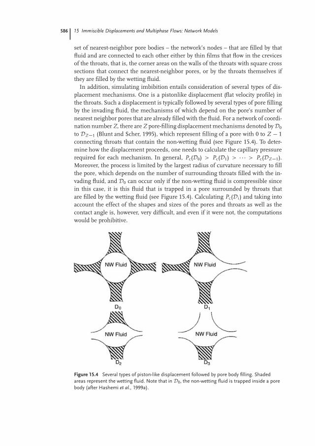
In addition, simulating imbibition entails consideration of several types of dis-placement mechanisms. One is a pistonlike displacement (flat velocity profile) inthe throats. Such a displacement is typically followed by several types of pore fillingby the invading fluid, the mechanisms of which depend on the pore’s number ofnearest neighbor pores that are already filled with the fluid. For a network of coordi-nation number Z, there are Z pore-filling displacement mechanisms denoted by D0

to DZ�1 (Blunt and Scher, 1995), which represent filling of a pore with 0 to Z � 1connecting throats that contain the non-wetting fluid (see Figure 15.4). To deter-mine how the displacement proceeds, one needs to calculate the capillary pressurerequired for each mechanism. In general, Pc(D0) > Pc(D1) > � � � > Pc(DZ�1).Moreover, the process is limited by the largest radius of curvature necessary to fillthe pore, which depends on the number of surrounding throats filled with the in-vading fluid, and D0 can occur only if the non-wetting fluid is compressible sincein this case, it is this fluid that is trapped in a pore surrounded by throats thatare filled by the wetting fluid (see Figure 15.4). Calculating Pc(Di ) and taking intoaccount the effect of the shapes and sizes of the pores and throats as well as thecontact angle is, however, very difficult, and even if it were not, the computationswould be prohibitive.

Figure 15.4 Several types of piston-like displacement followed by pore body filling. Shadedareas represent the wetting fluid. Note that in D0, the non-wetting fluid is trapped inside a porebody (after Hashemi et al., 1999a).

15.2 Simulating the Flow of Thin Wetting Films 587

To circumvent the difficulty, a parameterization of Pc(Di ) is used for describingthe advancement of the fluid, which is as follows. The mean radius of curvature Ri

for filling by the Di mechanism is (Blunt and Scher, 1995)

Ri D R0 CiX

j D1

A j x j , (15.10)

where x j is a random number distributed uniformly in (0, 1), A j is an input pa-rameter, and R0 is the maximum size of the adjacent throats. A j emulates theeffect of the pore space variables, and determines the relative magnitude of Pc(Di ).For example, if for j � 2, we set A j D 0, then the pore-filling events become inde-pendent of the number of the filled throats and, hence, the fluid advance is similarto the IP. If, on the other hand, A j are relatively large for large values of j, then themodel emulates the case of small or medium values of the ratio of pore and throatradii. In the model, Ri , computed by Eq. (15.10), is taken to be the pore radius forthe Di mechanism of pore filling. Thus, if one fluid is strongly wetting, the criticalcapillary pressure Pc for pore filling when the pore has i adjacent unfilled throatsis taken to be

Pc D 2σRi

, (15.11)

where σ is the interfacial tension between the two fluids.During imbibition, one also must consider the snap-off mechanism of throat

filling (see Chapter 14): as Pc decreases, the radius of curvature of the interfaceincreases, and the wetting films occupying the crevices of the walls swell. At somepoint, further filling of the crevices causes the radius of curvature of the interfaceto decrease, leading to instability and spontaneous filling of the center of the throatwith the wetting fluid. The critical capillary pressure for snap-off is given by

Pc D σrt

, (15.12)

which is always smaller than Pc D 2σ/rt for pistonlike displacement, implying thatsnap-off can occur only if pistonlike advance is topologically impossible becausethere is no neighboring pore filled with the invading fluid.

Therefore, to simulate imbibition and take into account the flow of thin wettingfluid films, consider a pore or a throat filled with the non-wetting fluid, and assumethat the wetting fluid is supplied by thin film flow along a crevice of length `. We ig-nore any pressure drop in the non-wetting fluid and in the portions of the networkcompletely saturated by the wetting fluid (a valid assumption if the capillary num-ber is small), but the pressure drop along the thin wetting layers in the crevices ofthe network is significant and cannot be neglected. The relation between the wet-ting fluid flow rate q and the pressure gradient for the thin films in the cornersis

q D � r4

�sµw

dPw

dx, (15.13)


where µw and Pw are the viscosity and local pressure of the wetting fluid, r is thelocal radius of curvature in the corner, and �s is a dimensionless conductance factorthat depends on the shape of the cross section of the throat and the boundaryconditions at the phase boundary. For example (Blunt and Scher, 1995), for squarecrevices, �s D 109 if there is no slip at the interface between the two fluids. Moregenerally, �s varies anywhere from 15 to 290 (Ransohoff and Radke, 1988). Weassume that, locally, the interface is in capillary equilibrium and, hence, Pw D�Pc D �σ/r , and that flow of the thin films (in the crevices) as well as �s areindependent of the time. Then, for the thin films, q D σ4/(µw�sP4

c )dPc/dx , thatis, flow of the thin wetting films is driven by a capillary pressure gradient in thefilms. Integrating the equation in (0, `), we obtain

Pc0 D Pcl

1 C 3

�s P3clqµw`

σ4

!� 13

, (15.14)

where Pc0 is the capillary pressure of the element (pore or throat) at the inlet of thecrevice, and Pcl is the local capillary pressure where the element is being filled – ei-ther by pistonlike throat filling or throat filling by snap-off, or by the Di mechanismof pore filling.

15.3Displacements with Two Invaders and Two Defenders

The models of two-phase flow and displacement described so far only involve onedisplacing fluid – the invader – and one displaced fluid – the defender – whereasin many problems, both at laboratory and field scales, one has a situation in whichthere are at least two invaders and two defenders. Recall from Section 14.8, that atthe end of the displacement processes described there, the displaced fluid exists on-ly in isolated blobs or clusters of finite sizes that can no longer be displaced by anyof the above displacement processes. In order to mobilize and displace such blobs,the Ca must be significantly increased, which would then give rise to three otherdisplacement processes that are quasi-static and dynamic displacement of blobs,both of which are time-dependent phenomena and steady-state dynamic displace-ment. The last process can be carried out if the displacing and displaced fluids aresimultaneously injected into the porous medium. Thus, simulating displacementswith two invading and two defending fluids is of practical importance. However,such a model is also motivated by other practical considerations.

Recall from Chapter 14, for example, that in a typical experiment for measuringthe RPs of two-phase flows, the porous medium is initially saturated with the non-wetting (or the wetting) fluid. Then, a mixture (not a solution) of both fluids ofa given composition is injected into the sample at a constant flow rate. The twofluids are uniformly distributed at the entrance to the medium, and the flow ismaintained until steady state is reached at which point the pressure drop alongthe sample is recorded that, together with the flow rates of the two fluids and the

15.3 Displacements with Two Invaders and Two Defenders 589

Darcy’s law, yield estimates of the RPs. Thus, measurement of the RPs involvessimultaneous invasion of a porous medium by two immiscible fluids.

As another example, consider two-phase flow in fractures. As described in Chap-ter 6, a natural fracture usually has a rough self-affine surface. Experimental obser-vations in horizontal fractures indicate (Glass and Norton, 1992; Glass and Nicholl,1995; Glass et al., 1995) that in two-phase flow through a fracture, when an inva-sion front encounters a zone characterized on average by much smaller apertures(the zone of the wetting fluid) or much larger ones (the zone of the non-wettingfluid), the invading front advances into that region at the expense of the already

invaded region. In other words, some apertures in the already invaded region arespontaneously re-invaded by the defending fluid to provide invading fluid for thenewly encountered zone. In addition, it has been observed that at low flow rates,gravity-driven fingers drain a distance behind the invading finger tip. Thus, two-phase fluid invasion in horizontal fractures involves simultaneous imbibition anddrainage of the apertures within the fractures.

Hashemi et al. (1998, 1999a,b) developed an IP model with two invaders and twodefenders. In simulating such a model, one must recognize that when the fluidclusters are pushed one after another, ` in Eq. (15.14) represents the minimumdistance between the element to be filled by the thin wetting films and the point atthe interface between the invading and defending clusters where the path lengththrough the elements completely filled with the wetting fluid is zero. Therefore,when a cluster of the non-wetting fluid pushes a wetting fluid cluster, one has` D 0, as there is no path of pores and throats that contain thin films of non-wetting fluid in the defender cluster. However, ` ¤ 0, if a cluster of the wettingfluid pushes a cluster of the non-wetting fluid since in this case, a thin film ofthe wetting fluid can participate in the displacement. If each throat is a channelof radius r and characteristic length d (e.g., the distance between two neighboringnodes), we rewrite Eq. (15.14) in dimensionless form using `� D `/d, u D q/d2,and P�

c D Pcr/σ to obtain

P�c0 D P�

c`

�1 C 3C P�3

c` `�� 1

3 , (15.15)

where C D �s(d/r)3(uµw/σ) D �s(d/r)3Ca, with Ca being the capillary numberfor the flow of thin wetting films. Assuming that the flow rate in each crevice isconstant (independent of the time), we consider the filling of an element with thewetting fluid and use Eq. (15.15), replacing ` with the minimum distance betweenthe filling element and the inlet of the filled one, where the path length throughthe throats completely filled with the wetting fluid is zero (i.e., only the paths thatconsist of the thin wetting films are counted in calculating `).

At time t D 0, the network is filled with the non-wetting fluid, and is assumedto be incompressible, so that its trapping by the wetting fluid is possible. A trappednon-wetting fluid cluster can be broken up into pieces only by flow of the wet-ting films (see below). A site is selected at random on one face of the network forinjection, and another site on the opposite face for production. Thus, the bound-ary condition in the direction of macroscopic displacement is a constant injection


rate. The motion of the injected fluid is represented by a series of discrete jumpsin which, at each time step, the invader displaces the defender from the availablepores through the least resistance path. In the presence of film flow through thecrevices and strongly wetting condition, all the pores are accessible to the wettingfluid, while in the case of no film flow, only the interface pores are accessible. Ateach stage, the pressure needed for flow of the invader from the injection site tothe production site through all the accessible pores is calculated by summing up thecapillary pressure differences of the pores through all the possible paths (see below).The path with the least pressure is then selected. This is completely different fromthe usual IP models in which only the interface pores are considered. If the wet-ting fluid is displacing the non-wetting one, then after the element is filled, forevery possible new path, the corresponding ` is recomputed (in the case of thenon-wetting fluid displacing the wetting fluid one has, ` D 0). If the number offilled throats adjacent to any of the pores has increased, the pore filling capillarypressures are updated to represent the proper Di mechanism.

Consider, for example, a situation in which the non-wetting fluid is in a clusterthat is connected to the inlet of the network, and is in contact with three wettingclusters, which we call WF1, WF2, and WF3. Suppose that the non-wetting fluidtries to displace the wetting fluid. Since there are three wetting fluid clusters thatare also in contact with one or several other non-wetting fluid clusters in “front”of them, which in turn touch other non-wetting fluid clusters including one thatis connected to the outlet of the network, one must consider all the possible pathsof the clusters that are pushing one another, and identify the one that requires theminimum pressure for the displacement from the point of the contact between theinlet non-wetting fluid cluster and the network’s outlet. To do so, one must identifyall the non-wetting clusters that are in contact with WF1, WF2, and WF3, whichwe refer to as the secondary clusters. Then, the tertiary clusters that are in contactwith the secondary clusters must also be identified, and so on, until all the possiblepaths from the inlet non-wetting cluster to the outlet are listed. As such, this is aproblem in combinatorial mathematics.

One then calculates the minimum pressure ∆P for displacing a wetting fluidcluster by a non-wetting cluster, and vice versa. Consider, first, the case in whichthe non-wetting fluid that is connected to the inlet of the network tries to displacea wetting cluster. In this case, only the elements (pores and throats) of the wettingcluster that are at the interface between the two types of clusters are accessible fordisplacement, as there is no flow of the non-wetting films in any element. Let 1denote an interfacial element between the invader (the non-wetting fluid) and thedefender cluster (the wetting fluid), and 2 denote the outlet point of the wettingcluster to another non-wetting cluster. Recall that the pressure drop between theinlet and outlet elements is ∆P12 D Pnw1 � Pw2, and that Pnw1 � Pw1 D Pc1.Therefore, ∆P12 D Pw1 � Pw2 C Pc1. If we assume that there is no pressure drop inthe wetting cluster (which is true at low to moderate Ca, then ∆P12 ' Pc1. Thus,we calculate ∆P12 for all the interfacial elements between any two non-wetting andwetting clusters that are in contact. Then, for a path that starts from the inlet non-wetting cluster to the outlet of the network, we write the total required pressure

15.3 Displacements with Two Invaders and Two Defenders 591

drop (∆P )path as a sum over all such ∆P12s for the non-wetting and wetting clustersthat are in contact, being pushed by one cluster on one side (the inlet point 1) andpushing another cluster at another side (the outlet point 2), and belonging to thepath:

(∆P )path D (∆P12)cluster 1 C (∆P12)cluster 2 C (∆P12)cluster 3 C � � �DX

i

(Pc1)cluster i , (15.16)

where cluster 1 is in contact with cluster 2, which is in contact with cluster 3, and soon. In dimensionless form, each term of Eq. (15.16) is calculated using Eq. (15.15).One then selects the path for which (∆P )path is minimum, and keep in mind thatwhen a non-wetting fluid cluster pushes a wetting fluid one, one must calculate thecapillary pressure for all the interfacial elements (i.e., all the Pc1) between the twoclusters in order to determine the minimum ∆P12.

Next, consider the case in which the wetting fluid that is connected to the networkinlet attempts to push a non-wetting cluster. The general method of selecting thedisplacement path is the same as before, but two distinct cases must be considered.

1. Suppose that there is no flow of thin wetting films in the crevices. Using thesame arguments and notation as above, it is straightforward to show that forany non-wetting cluster that is being pushed by the wetting fluid and is alsopushing another wetting cluster, ∆P12 D �Pc1, assuming again that the pres-sure in the non-wetting cluster is the same everywhere. The minimum pressureis again determined by considering (∆P )path for all the possible paths.

2. If flow of thin wetting films exists, then the wetting fluid can reach any partof any cluster of the defending non-wetting fluid. One must now calculate theminimum Pc for filling every element within the non-wetting fluid cluster, andalso those that are at the interface with the wetting fluid. Let one denote aninterfacial element between the invading wetting cluster and the defendingnon-wetting cluster, two be a point inside (a pore of) the non-wetting cluster,and three denote the outlet element of the non-wetting cluster next to anoth-er wetting cluster. Since the minimum of such Pcs corresponds to the mini-mum ` (see Eq. (15.15)), then point two is the location of the element with-in the non-wetting cluster and one is the point at the interface between thewetting and non-wetting fluids that has the smallest distance to that element.Thus, one has ∆P13 D Pw1 � Pnw3, and Pc1 D Pnw1 � Pw1 and, therefore,∆P13 D Pnw1 � Pnw3 � Pc1. Recall that Pc1 is related to the capillary pressureof the element located at two through Eq. (15.15). Since Pnw1 D Pnw2 D Pnw3,we obtain ∆P12 D �Pc1. Therefore, in all the cases, the individual ∆P12s onlydepend on the inlet condition of the clusters, and are independent of the outletconditions. Note that in both cases, a distinct ` is associated with each possiblepath.

At the end of imbibition, the network is invaded with both the wetting and non-wetting fluids, which initiates the fractional flow displacement (FFD). The frac-


tion f w of the wetting fluid in the injected mixture is fixed. At the early stagesof the FFD, there is a continuous path of the wetting fluid through the network,while the non-wetting fluid remains entrapped in its isolated clusters so that theinjected wetting fluid can exit from the network’s opposite face, whereas the non-wetting fluid accumulates in the network. After successive injections, the injectednon-wetting fluid joins its entrapped clusters and, thus, larger clusters of the non-wetting fluid are generated progressively. The invader fluids push many clusters ofthe non-wetting and wetting fluids, and the wetting fluid clusters that are alreadyin the network.

To determine the path of the mobilized clusters from the inlet to the outlet, wefirst identify all the clusters and their neighbors. Then, all the possible paths of theclusters from the injection site to the production site are identified and stored in alist. Using Eq. (15.15), the pressure required to mobilize each of the clusters in thelist is calculated for each path. The path that requires the least pressure is selectedas the flow path between the inlet and the outlet of the network. This representsan important difference between the model for the FFD and the usual IP modelsin which only the throat with the smallest resistance at the interface is considered.The difference is necessitated by the fact that mobilization of an entrapped fluidcluster is different from simple displacement of one fluid by another in a pore orthroat.

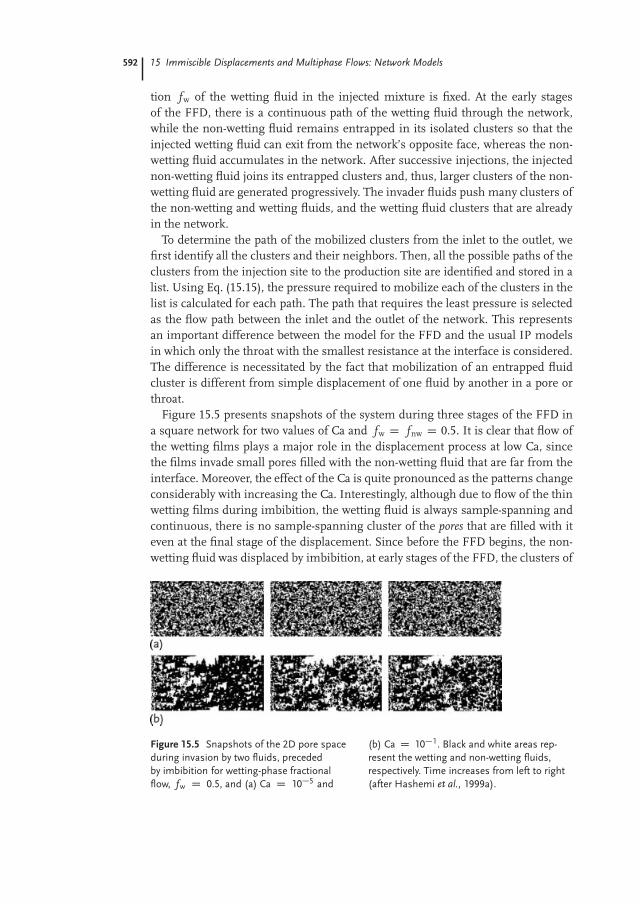
Figure 15.5 presents snapshots of the system during three stages of the FFD ina square network for two values of Ca and fw D fnw D 0.5. It is clear that flow ofthe wetting films plays a major role in the displacement process at low Ca, sincethe films invade small pores filled with the non-wetting fluid that are far from theinterface. Moreover, the effect of the Ca is quite pronounced as the patterns changeconsiderably with increasing the Ca. Interestingly, although due to flow of the thinwetting films during imbibition, the wetting fluid is always sample-spanning andcontinuous, there is no sample-spanning cluster of the pores that are filled with iteven at the final stage of the displacement. Since before the FFD begins, the non-wetting fluid was displaced by imbibition, at early stages of the FFD, the clusters of

Figure 15.5 Snapshots of the 2D pore spaceduring invasion by two fluids, precededby imbibition for wetting-phase fractionalflow, fw D 0.5, and (a) Ca D 10�5 and

(b) Ca D 10�1. Black and white areas rep-resent the wetting and non-wetting fluids,respectively. Time increases from left to right(after Hashemi et al., 1999a).

15.4 Random Percolation with Trapping 593

the non-wetting fluid are isolated. However, as the invasion by both fluids proceeds,they become connected progressively and form larger clusters. At some point dur-ing the FFD, both fluid phases become continuous – the non-wetting fluid via thesample-spanning cluster of the pores and throats that it occupies, and the wettingfluid through the thin films and the pores that it has invaded. This is a novel fea-ture of invasion by two fluids in 2D with flow of thin films, and is in contrast withthe usual IP models in which there is only one continuous fluid phase during thedisplacement.

15.4Random Percolation with Trapping

Random percolation with trapping was developed first by Sahimi (1985) and Sahi-mi and Tsotsis (1985) to model catalytic pore plugging of porous media. In theproblem that they studied, the pores of a porous medium plug as the result of achemical reaction and deposition of the solid products on the surface of the pores.Large pores take a long time to be plugged, and if they are surrounded by smallpores that quickly plug, they become trapped and cannot be reached by the reac-tants penetrating the porous medium from outside.

Accurate computer simulations of Dias and Wilkinson (1986), who proposed thesame model for two-phase flow problems in porous media, indicated that mostproperties of random percolation with trapping in both 2D and 3D are the same asthose of random percolation. The pore size distribution (or threshold capillary pres-sures for pore invasion) that was considered by Dias and Wilkinson was, however,narrow (a uniform distribution in (0, 1)). If the pore size distribution is, howev-er, broad (as in the problem studied by Sahimi and Tsotsis), percolation with andwithout trapping may not necessarily have the same properties.

15.5Crossover from Fractal to Compact Displacement

As Figure 15.2 indicates, the RP to the non-wetting phase during the primary im-bibition by a strongly wetting fluid only vanishes at Srnw D 0, implying that thenon-wetting phase is completely expelled from the medium and that the wettingphase fills up the pore space. The conclusion is that imbibition is an essentiallycompact displacement. During drainage by a completely non-wetting fluid, however,the RP to the wetting fluid phase vanishes at a finite value of Srw, implying that thenon-wetting fluid phase does not fill up the porous medium and a fractal clusteremerges. Such differences between imbibition and drainage were already predictedby the random percolation model of Heiba et al. (1982, 1992), and was also nicelydemonstrated by Lenormand and Zarcone (1984) who used a 2D etched network,injected mercury into the system (drainage), and then withdrew it (imbibition).


The cluster formed during imbibition was totally compact and filled up the etchednetwork.

A definitive study of the problem was made by Cieplak and Robbins (1988, 1990).In their study, the porous medium was represented by a 2D array of disks with ran-dom radii where the underlying network was either a triangular or a square net-work with the disks’ centers being at the network’s sites. The limit of low capillarynumber Ca was considered, and the displacement dynamics was modeled as a step-wise process where each unstable section of the interface moved to the next stableor nearly stable configuration. The simulations of Cieplak and Robbins indicatedthat there are three basic types of instability and the corresponding mechanisms ofthe advancement of the interface.

1. Burst, which happens when at a given capillary pressure Pc, no stable arc con-nects two disks and, therefore, the interface simply jumps forward to connectto the nearest disk.

2. Touch, which happens when an arc that connects two disks, intersects anotherdisk at a wrong contact angle θ , in which case the interface connects to thethird disk.

3. Overlap, which happens when two nearby arcs overlap. There is no need for thedisk to which both arcs are connected and, thus, it may be removed from theinterface.

Figure 15.6 illustrates the three mechanisms. To simulate the advancement of theinterface, the capillary pressure Pc is fixed and the stable arcs are identified. If in-stabilities are found, local changes are made to remove them. Then, Pc is increased

Figure 15.6 Three kinds of growth and instability that occur during an immiscible displacementin a porous medium: Burst (a); touch (b); overlap (c) (after Cieplak and Robbins, 1990).

15.5 Crossover from Fractal to Compact Displacement 595

slightly, the interface is advanced, the possible instabilities are removed again, andso on. As in the TIP, if the invading fluid surrounds a blob (cluster) of the displacedfluid, it is kept intact for the rest of the simulation. If all the disks have the sameradius, the resulting patterns are very regular and faceted, and preserve the sym-metry of the underlying network, in agreement with the experiments of Ben-Jacobet al. (1985).

However, when the radii of the disks are randomly distributed, then the structureof the invasion cluster depends on the contact angle θ . To quantify the effect of θ ,we define an interface width w by w (L) D h[h(x ) � hhiL]2i1/2, where h is the heightof the interface at position x, and hhiL is its average over a horizontal segment oflength L. When θ � 180ı (i.e., drainage), then the displacement represents anIP and w is of the order of pore size. Cieplak and Robbins (1988, 1990) showed,however, that as θ decreases, the invasion cluster becomes more compact and w

increases (see Figure 15.7). At a critical contact angle θc, w diverges according to apower law

w � (θ � θc)�νθ , (15.17)

where νθ ' 2.3. The critical angle θc was found to depend on the porosity φ of theporous medium; for example, θc ' 29ı for φ D 0.322, and θc ' 69ı for φ D 0.73.The exponent νθ was found to be universal (independent of the distribution of thedisks’ radius). The compactness of the cluster for θ < θc is consistent with theimbibition picture described above.

The divergence of w at θc is clearly due to the transition from fractal to compactdisplacement. For large θ , the interface advances mainly by burst, similar to theIP, and its pattern is independent of θ . However, as θ ! θc, the overlap and touchincidents become more important, and the interface becomes unstable for almost

Figure 15.7 Displacement patterns for θ D 179ı (a) and θ D 58ı (b) (after Cieplak andRobbins, 1990).


any configuration of the local geometry. Thus, the growth pattern of the interfacechanges and, hence, w diverges.

15.6Pinning of a Fluid Interface

The structure of the fluid interface during imbibition is interesting and differentfrom that during drainage. The invading fluid cluster during imbibition is com-pact, but capillary forces lead to random local pinning of the interface that resultsin an interface with a rough self-affine structure demonstrated by the experimentsof Rubio et al. (1989) and Horváth et al. (1991a). The self-affinity of such rough in-terfaces was first alluded to by Cieplak and Robbins (1988), but was not quantified.

Rubio et al. (1989) performed their experiments in a thin (2D) porous mediummade of tightly packed clean glass beads of various diameters. Water was injectedinto the porous medium to displace the air in the system. The motion of the inter-face was recorded and digitized with high resolution. The experiments of Horváthet al. (1991a) were very similar (see below). However, before embarking on an anal-ysis of the results of Rubio et al. (1989) and Horváth et al. (1991a), let us reviewbriefly the dynamics of rough surfaces and interfaces.

According to the scaling theory of Family and Vicsek (1985) for growing roughsurfaces, one has the following scaling form at time t,

h(x ) � hhiL � t � f

x

t�α

!, (15.18)

where α and � are two exponents that satisfy

α C α�

D 2 , (15.19)

and the scaling function f (u) has the properties that j f (u)j < c for u � 1, andf (u) � Lα f (Lu) for u � 1, where c is a constant. It is then straightforward to see

that

w (L, t) � t � g

�t

Lα�

�, (15.20)

where g(u) is another scaling function and, therefore,

w (L, 1) � Lα . (15.21)

Note that w (L, t) is a measure of the correlation length along the direction of inter-face growth. Note also that α is the same as the roughness or Hurst exponent Hdefined and described in Chapters 5, 6, and 8.

A variety of surface growth models and the resulting dynamical scaling can bedescribed by the stochastic differential equation proposed by Kardar et al. (1986)

@h

@tD σr2

Th C 12

v jrhj2 C N (r , t) , (15.22)

15.6 Pinning of a Fluid Interface 597

where σ is the surface tension, v is the growth velocity perpendicular to the inter-face, and N is a random noise. Kardar et al. (1986) considered the case in whichthe noise was assumed to be Gaussian with the correlation

hN (r, t)N (r 0, t)i D 2Aδ(r � r0, t � t0) , (15.23)

with A being the amplitude of the noise. For the KPZ model, it has been proposedthat (Kim and Kosterlitz, 1989)

α D 2(d C 2)�1 , � D (d C 1)�1 , (15.24)

for a d-dimensional system. Another stochastic equation was proposed by Koplikand Levine (1985):

@h

@tD σr2

Th C v C AN (r, h) , (15.25)

a linear equation but with a noise that is more complex than that of the KPZ equa-tion. For this model, the numerical work of Kessler et al. (1990) indicated thatα(d D 2) ' 0.75.

It is then straightforward to see why pinning of the fluid interface may occur byconsidering Eq. (15.25) in zero transverse dimension,

@h

@tD v C AN (h) . (15.26)

If v > ANmax, where Nmax is the maximum value of N , then @h/@t > 0, and the in-terface always moves with a velocity fluctuating around v. If, however, v < ANmax,the interface will eventually arrive at a point where v C AN D 0, and is pinnedthere. Therefore, for a fixed v, there must be a pinning transition at some finitevalue of A. Indeed, Stokes et al. (1988) performed fluid displacement experimentsin random packs of monodisperse glass beads in pyrex tubes and measured thecapillary pressures at which such a pinning transition takes place.

From their experiments, Rubio et al. (1989) found that α ' 0.73, significantlydifferent from α D 1/2, predicted by Eq. (15.24), though consistent with the resultof Kessler et al. (1990). Horváth et al. (1990) reanalyzed Rubio et al.’s data and ob-tained α ' 0.91, which is larger than all other values. They also carried out theirown experiments in a Hele-Shaw cell, packed randomly and homogeneously withglass beads, and displaced the air in the pore space with a glycerol-water mixture,and obtained α ' 0.81 and � ' 0.65. Although their estimate of α was close toRubio et al.’s as analyzed by Horváth et al. (1990), and although the estimates sat-isfy scaling relation (15.19), they were significantly different from the predictionsof Eq. (15.24), but their α is consistent with Kessler et al.’s result. Martys et al.

(1991) employed the model of Cieplak and Robbins (1988) described earlier andshowed that below the critical angle θc, one has α ' 0.81, in perfect agreementwith Horváth et al. (1991a)’s estimate.

How can one explain these results? To our knowledge, no satisfactory explana-tions have been proposed. Zhang (1990) proposed a modification of the KPZ model


in which the distribution of the noise amplitude is of power-law form

P(A) � A�(µnC1) . (15.27)

Horváth et al. (1991b) then showed that the aforementioned experimental data canbe fitted with µn ' 2.7. A more plausible explanation was proposed by Nolle et

al. (1993). They calculated the local fluid velocities at the interface and showedthat they satisfy a power-law distribution similar to Eq. (15.27) with µn ' 2.7, inagreement with the estimate of Horváth et al. (1991b). Let us also note that Barabásiet al. (1992) extended the imbibition experiments to three dimensions, and reportedthat α ' 0.5.

15.7Finite-Size Effects and Devil’s Staircase

Most of the theoretical discussion so far has been limited to systems that are es-sentially of infinite extent. If the system is of finite size, the dependence of itsmacroscopic properties on its linear size L can be investigated using the finite-sizescaling described in Chapter 3. So, let us describe the effect of the linear size of afinite porous sample on its capillary pressure and the RPs. Thompson et al. (1987b)measured the electrical resistance of a porous medium during mercury injection(drainage) and showed that the resistance decreases (the permeability increases)during the injection process in steps on the so-called Devil’s staircase. Their dataare shown in Figure 15.8. The steps were irreversible in that small hysteresis loopsdid not retrace the steps, and were not reproduced on successive injections. Whenthe number N∆R of the resistance steps larger than ∆R was plotted versus ∆R , apower-law relation was found,

N∆R � (∆R)λR . (15.28)

with 0.57 λR 0.81. The magnitude of λR presumably depends on the strengthof the competition between the capillary and gravitational forces: λR ' 0.57 sig-nifies the limit of no gravitational forces, whereas λR ' 0.81 represents the limit

Figure 15.8 Resistance of a sandstone versus the injection pressure during mercury porosime-try (after Thompson et al., 1987b).

15.8 Displacement under the Influence of Gravity: Gradient Percolation 599

in which gravitational forces are prominent. Based on the stepwise decrease of theresistance and the apparent first-order (discontinuous) phase transition (see Fig-ure 15.8), Thompson et al. (1987b) concluded that mercury injection should not bemodeled by percolation that usually represents a second-order phase transition, thatis, one that is characterized by a continuous vanishing or divergence of a physicalquantity, for example, the permeability or conductivity, as a the percolation thresh-old is approached.

However, simulation of the same process by Katz et al. (1988), Roux and Wilkin-son (1988), and Sahimi and Imdakm (1988), and related simulation of Batrouni et

al. (1988) indicated that such a stepwise decrease in the resistance can be predict-ed by a (random or invasion) percolation. The reason for the stepwise decrease inthe sample resistance is that in a finite sample, penetration of any pore by mercurycauses a finite change in the resistance. As the sample size increases, however, thesize of the step change decreases, such that for a very large sample, the steps wouldvanish and the resistance curves become continuous and smooth. In fact, using apercolation model, Roux and Wilkinson (1988) showed that for a 3D porous medi-um of linear size L,

N∆R � L

3(µp�ν)µpC3ν (∆R)

�3ν

µpC3ν , (15.29)

where µp and ν are, respectively, the critical exponents of the conductivity of theporous medium and the percolation correlation length (see Chapter 3). Thus, λR D3ν/(µp C3ν) ' 0.57, which agrees well with the experimental result in the absenceof gravity.

15.8Displacement under the Influence of Gravity: Gradient Percolation

In all the discussions so far, the effect of gravity on immiscible displacements hasbeen ignored. However, in 3D porous media, the effect of gravity cannot be neglect-ed. The hydrostatic component of the pressure adds to the applied one, which thencreates a vertical gradient in the effective injection pressure. Due to the gradient,the fraction of pores that are accessible to the displacing fluid decreases with theheight of the system. A modification of the IP model proposed by Wilkinson (1984),and developed further by Sapoval et al. (1985) and Gouyet et al. (1988), succeededin taking into account the effect of gravity. However, before describing the models,let us briefly describe a few experimental studies regarding the effect of gravity.

Clément et al. (1987) and Hulin et al. (1988b) used the following procedure tostudy gravitational effects. They injected Wood’s metal, which is a low-meltingpoint liquid alloy, into the bottom of a vertical and evacuated crushed-glass col-umn. The experiments were carried out at low capillary number Ca by controllingthe flow velocity v. After the front reached a given height, the injection was stoppedand the liquid was allowed to solidify. The horizontal sections of the front corre-sponding to various heights were then analyzed, and the correlation function C(r)


(see Chapter 4) of the metal distribution in the horizontal planes was determinedin order to see whether a fractal structure had been formed. Another series of ex-periments were carried out by Birovljev et al. (1991) in a 2D porous medium. Theyused transparent models consisting of a monolayer of 1 mm glass beads placed atrandom and sandwiched between two plates. The system was filled with a glycerol-water mixture, which was displaced by air invading the system at one end.

The competition between gravity and capillary forces is usually quantified by theBond number Bo, already defined in Chapter 14 and repeated here:

Bo D ∆�g`2g

σ, (15.30)

where ∆� is the density difference between the two fluids, g is the gravity, and`g is the typical size of the grain. Wilkinson (1984) showed that in an immiscibledisplacement under gravity, the correlation length g does not diverge, unlike inrandom and invasion percolation that have a diverging correlation length p (seeChapter 3), but that it reaches a maximum given by

g � Bo�ν

1Cν , (15.31)

where ν is the exponent that characterizes the divergence of the percolation corre-lation length p (see Chapter 3). Thus, g � Bo�0.47, and g � Bo�4/7 in 3D and2D, respectively. In 3D, there is a transition region where both fluids (displacingand displaced) may percolate in the porous media, the width w of which is given by

w � Bo�1 . (15.32)

Similar results were derived by Sapoval et al. (1985) and Gouyet et al. (1988) in thecontext of gradient percolation, which is a model in which a gradient G is imposedon the occupation probability p in one direction of the network. The model had, infact, been considered earlier by Trugman (1983) who called it a graded percolation.Sapoval et al. and Gouyet et al. used scaling arguments similar to Wilkinson’s toshow that

g � G�

ν1Cν , (15.33)

which is completely similar to Eq. (15.31) in which the Bound number Bo hasbeen replaced with G. The 3D experiments of Hulin et al. (1988b) and the 2D ex-periments of Birovljev et al. (1991) were completely consistent with the predictions.For example, Birovljev et al. (1991) reported that g � Bo�0.57, where the exponent0.57 agrees perfectly with the prediction, ν/(1 C ν) D 4/7 ' 0.57.

Wilkinson (1984) also derived an important result regarding the effect of gravityon the residual oil saturation (ROS). He showed by a scaling argument that thedifference Sro � S0

ro, where Sro is the ROS for Bo ¤ 0 and S0ro is the corresponding

value when Bo D 0 is given by

Sro � S0ro � BoλB , (15.34)

15.9 Computation of Relative Permeabilities 601

where λB D (1 C �)/(1 C ν), with � being the standard percolation exponent forthe fraction of accessible pores near the percolation threshold, or the ROS (seeChapter 3). Thus, Eq. (15.35) predicts that in a 3D porous medium, Sro � S0

ro �Bo0.74. In addition, Wilkinson (1984) proposed a simple model for simulating theIP under the influence of gravity.

15.9Computation of Relative Permeabilities

The two most important properties of two-phase flow in a porous medium are theRPs and capillary pressure. Many empirical correlations have been proposed in thepast that relate such properties to a measurable parameter, for example, the fluidsaturation. Several equations have also been rigorously developed based on simplemodels of porous media. However, such equations are as valid as the model usedin their development. Two of the models, namely, the sphere pack and bundle oftubes, are too simple – the former is not appropriate for consolidated porous media,while the latter does not take into account the effect of the pores interconnectivity.As a result, the equations derived based on the two models fail to predict the data.Agreement between the theory and data is achieved with such models by insertingadjustable parameters of doubtful physical significance.

Fatt (1956a,b,c) pioneered the pore-network approach by using a regular 2D net-work to determine capillary pressure and the RPs. However, as described in Chap-ter 3, it was the work of Larson et al. (1977) that ignited the use of pore networkmodels in modeling of two-phase flow in porous media. The paper by Heiba et

al. (1982) demonstrated how the RPs are accurately computed using pore networkmodels and concepts from percolation theory.

15.9.1Construction of the Pore Network

It is possible to carry out flow simulations directly on the chaotic pore space by solv-ing the Naviér–Stokes equation numerically (Adler et al., 1990, 1992), or by usinga lattice-Boltzmann technique (see Chapters 9, 11, and 12). However, such compu-tations can only be done at considerable computational cost. It is, therefore, con-venient to construct a pore network that mimics the essential features of the porespace that are relevant to fluid flow. Such network models were already describedin Chapters 7, 10, and 11 for single-phase flow and transport. One can reconstructthe network by transforming the reconstructed pore space into a network (Bakkeand Øren, 1997).

For predictive modeling, two approaches may be used to characterize the porenetwork. (1) A simpler approach uses a regular network of capillary elements torepresent a system of pores and throats. (2) One tries to model the random topolo-gy of the pore space directly by either X-ray computed tomography, a process-basedtechnique, or a statistical technique. The main advantage of regular network mod-


els is their computational simplicity. Not much information is needed to describethe pore system. However, regular networks, although used extensively, have sev-eral shortcomings. As already pointed out, cylindrical throats do not support thepresence of more that one phase. Perhaps the most fundamental disadvantage of aregular network is that the simulation results may not be directly compared with ananalogous physical pore space (Fischer and Celia, 1999; Sok et al., 2002). To makea direct comparison, such parameters as the coordination number and pore sizedistribution should be tuned to match the “easily” measured data, such as, the cap-illary pressure, and then the model can be used to predict those properties that aremore difficult to measure, for example, the RPs. One may also use irregular net-works built based on regular ones (Ghassemzadeh et al., 2001; Ghassemzadeh andSahimi, 2004a,b), Voronoi networks (Sahimi and Tsotsis, 1997; Fenwick and Blunt,1998a,b; Blunt and King, 1990, 1991; Dadvar and Sahimi, 2003), Delaunary trian-gulations (Blunt and King, 1990, 1991) and irregular networks that allow a variablecoordination number (Lowry and Miller, 1995). Another approach is to use non-destructive X-ray computed microtomography (Spanne et al., 1994) to image the3D pore space directly at a resolution of around a micron, which is not, however,sufficient to image the sub-micron size pores that are abundant in carbonates andcan only be imaged by such 2D techniques as scanning electron microscopy.

Geometrical properties, for example, the porosity and the two-point correlationfunction, can be measured from 2D thin sections with high resolution, and usedto generate – to reconstruct – a 3D image with the same statistical properties. Theadvantage of the method is its generality, allowing a wide variety of porous media tobe reconstructed. It has been shown, however, that the two-point correlation func-tions and statistics often fail to reproduce the long-range connectivity of the porespace. One may use multiple-point statistics based on 2D thin-sections as train-ing images in order to generate geologically realistic 3D pore space representationsthat preserve the long-range connectivity of the pore structure (see also Chapter 7).

15.9.2Pore Size and Shape

The shapes attributed to pores and throats have a significant effect on the flowand transport properties. In the early pore network models, the pore bodies wereeither not modeled explicitly at all (they simply connected throats), or assumed tobe spherical or cylindrical. However, micromodel experiments (Lenormand et al.,1983) demonstrated that in pores with a rough or angular cross section, the wettingphase may occupy the crevices in layers of order of micron across, and provide extraconnectivity (see Section 15.2), while the non-wetting phase occupies the bulk ofthe pore space. To capture this feature, throats with square or triangle cross sectionsshould be used. One may define a shape factor Sf by

Sf D S

P2, (15.35)

where S and P are, respectively, the cross-sectional area and perimeter of the pore.


The irregular triangle is not an exact replica of real pores, though it does havethe same range of shape factors as those measured for real porous media. Theassumption is that the triangular shape correctly reproduces the balance betweenthe flow in corners (or roughness) and flow in pores’ centers. Consider an irregulartriangle with corner half angles of α1, α2, and α3, with 0 α1 α2 α3 π/2.α1 and α2 are associated with the base of the triangle, and R D 2S/P D 2P Sf isthe radius of the inscribed circle. If three rays connect the circle’s center to the threevertices, and three lines from the center are drawn perpendicular to the triangle’sthree bases, then S D R2 P3

iD1 cot α i . Recalling that, α3 D 1/2π � (α1 C α2), oneobtains

Sf D 14

3X

iD1

cot α i

!�1

D 14

tan α1 tan α2 cot(α1 C α2) . (15.36)

Thus, for such a triangle, Sf varies from zero for slit-like elements top

3/30 '0.048113 for equilateral triangles. A given Sf corresponds to a range of triangleswith the limits of the range being α2,min and α2,max that, in turn, correspond to thetriangles with α2,min D α1 D α and α2,max D 1/4π � 1/2α1. Note that the shapefactor for rectangular cross sections with all corner half angles being equal to 1/4πis 1/16, whereas for circular cross sections, Sf D 1/4π.

The assumption of an effective circular cross section is reasonable for predictingsingle-phase properties, and the RP of the non-wetting phase that resides in thecenters of the larger pores. For multiphase flow, the capillary entry pressure fornon-wetting phase depends on the minimum effective radius along the throat, andfor the saturation computation, the pore volumes are essential. Thus, independentexpressions for capillary entry pressure, volume and conductance of the network el-ements must be considered and, consequently, three different radii are important:an inscribed radius to determine capillary pressure at which a non-wetting phaseenters the element; a radius that controls the volume, and a hydraulic radius thatcontrols fluid conductance. A variety of pore shapes have been used in the past, in-cluding fractal models of roughness (Tsakiroglou and Fleury, 1999a,b; Tsakiroglouand Payatakes, 2000), grain boundary pore shapes (Man and Jing, 2001; Mani andMohanty, 1998), squares (Blunt, 1998; Fenwick and Blunt, 1998a,b; Hashemi et al.,1998, 1999a,b; Dillard and Blunt, 2000), and triangles (Øren et al., 1998; Hui andBlunt, 2000; Piri, 2003; Piri and Blunt, 2004, 2005a,b).

15.9.3Quasi-Static and Dynamic Pore Network Models

Two general types of network models may be identified: those for quasi-static dis-placements that fruitfully use the various percolation models, and the dynamicdisplacement models. Quasi-static models impose a capillary pressure on the net-work and calculate the final, static position of all the fluid–fluid interfaces, neglect-ing dynamic aspects of pressure propagation within the model and the interfacedynamics. Dynamic models typically impose a specified inflow rate for one of the


fluids and calculate the subsequent transient pressure response and the associatedinterface positions. Older pore network simulations for computing the RPs includethose of Lin and Slattery (1982), Mohanty and Salter (1982), Sahimi et al. (1986a),Blunt and King (1990, 1991), and Jerauld and Salter (1990).

In his model, Wise (1992) removed the throats with the smallest radii froma regular cubic network until the computed capillary pressure (see Chapter 4)matched the data. Rajaram et al. (1997) used a network with spatial correlationbetween the throat radii and optimized both the pore size distribution and thecorrelation parameters to obtain good agreement with the capillary pressure da-ta. Fischer and Celia (1999) used the same approach, but obtained poor predic-tions for the RPs. Since the Pc data are not always available, and because the opti-mal parameters obtained by matching the data and simulation are not necessarilyunique (Vogel, 2000), other alternatives have been developed for using the Pc da-ta when statistical properties of a porous medium are mapped onto the networkmodels.

Vogel and Roth (1998, 2001) obtained pore size distribution and pore connec-tivity from reconstructed samples of unconsolidated soils using multiple 2D thinsections. Hilpert et al. (2003) used a similar approach, though by using a cubic net-work and introducing cross correlation between the throats sizes connected to asingle pore. They were able to predict with reasonable accuracy data for both theprimary drainage and imbibition capillary pressures for several sphere packs.

Tsakiroglou and Payatakes (2000) combined extracting statistical properties fromreconstructed samples with conditioning to capillary pressures from mercury in-trusion and retraction. First, the pore size distribution and connectivity informa-tion were extracted from thin section analysis with throat size distribution esti-mated from the experimental capillary pressures. The parameters were then opti-mized along with the coordination number distribution using a cubic network un-til a satisfactory match with both intrusion and extraction capillary pressures wereobtained. The numerical results for both the capillary pressure and single-phasepermeability agreed well with the data.

Sok et al. (2002) compared flow and transport properties computed with topolo-gically-equivalent networks to those based on a face-centered cubic. Even whenthe spatial and cross correlation for the pore and throat sizes as well as the cor-rect distribution of coordination numbers were used, the regular networks yield-ed poor predictions of both the invasion pattern and the residual saturations.The conclusion was that those parameters that can be obtained from the recon-structed porous medium are not sufficient for reliable predictions of flow andtransport properties, and that additional higher-order topological information isneeded.

The predicted flow properties not only depend on the network topology and poresize distribution, but also on how each individual pore element is represented andhow much pore-scale physics they can accommodate. Most of the network modelshave used cylindrical tubes to represent the throats. Using a biconocal shape ratherthan a uniform cylinder for throats, Reeves and Celia (1996) argued that more ac-curate calculations can be carried out. As already pointed out, a major shortcoming


of cylindrical pores is their inability to contain more than one fluid, whereas it isclear that thin films of the wetting layer has a significant effect on flow properties.It was partly for this reason that Hashemi et al. (1998, 1999a,b) developed their porenetwork model that was described in detail in Section 15.3. They used pores andthroats with square cross sections.

Kovscek et al. (1993) suggested using star-shaped tubes in order to capture theeffects of wetting layers, which is also the same cross-sectional shape that was usedby, for example, Man and Jing (2001). To incorporate the measured quantities of thehighly irregular pore space – cross-sectional area, radius, and perimeter length –into the network model, a dimensionless shape factor G was suggested by Masonand Morrow (1991). A further advantage of such an approach is that not only willit correct for layer volume and conductivity, but that the calculated capillary entrypressure will also be a direct function of the pore shape (Mason and Morrow, 1991;Ma et al., 1996; Øren et al., 1998; Patzek, 2000; Valvatn and Blunt, 2003; Piri andBlunt, 2002, 2004, 2005a,b).

As already pointed out, the wetting physics of a porous medium strongly influ-ences the RPs and capillary pressure and, therefore, including the wetting effectin the pore network model has also been an active research area. The first attemptin this area was undertaken by Heiba et al. (1983). More complex is the issue ofhow mixed wettability (see Chapter 14) is distributed at the pore scale. Kovscek et

al. (1993) proposed a model whereby the smaller pores become oil-wet while thelarger ones remain water-wet. Moreover, visual observation of fluid distribution atthe pore scale using cryo- and environmental scanning electron microscopy (Fassi-Fihri et al., 1991; Combes et al., 1998; Durant and Rosenberg, 1998) suggested thatthe distribution of clay, in particular kaolinite, plays a very important role in deter-mining what parts of the rock are oil-wet.

McDougall and Sorbie (1995, 1997) investigated trends in the RP as well as oil re-covery efficiency with a fairly simple network model that did not explicitly includethe wetting layers. Dixit et al. (1998, 1999, 2000) used the same network modelsof McDougall and Sorbie (1995) in order to introduce a wettability classificationsystem, relating the recovery from mixed-wet porous media to aging and fractionof oil-wet pores. Using the capillary pressures of various flooding cycles, they sug-gested that it is possible to determine whether oil-wet pores are correlated to thepore size, or are simply randomly distributed.

Blunt (1997, 1998) and Hashemi et al. (1998, 1999a,b) used square pores andthroats to explicitly model the flow of the thin wetting layers. Using simple geolog-ical considerations, expressions for the capillary pressure for various filling events(see Section 15.2) described by Lenormand et al. (1983) were developed. In eachelement (pore or throat), multiple wetting conditions were allowed to exist, withthe corners remaining water-wet while the center becoming oil-wet. The effect onthe RPs of a wide range of wetting conditions was investigated.

Very limited mixed-wet experimental RP data have been predicted using porenetwork models (Øren et al., 1998). Jackson et al. (2003) used geologically realisticnetworks of Berea sandstone to obtain the trends in the experimental recoveries.


They assumed that all the invaded pores following the primary drainage becameoil-wet. The experimentally measured wettability indices were then matched byvarying the distribution of oil-wet contact angles. Øren and Bakke (2003) obtainedquantitative agreement with the experimental recoveries, and introduced a methodfor estimating the oil-wet fraction and the contact-angle distributions using themeasured wettability indices. Valvatn and Blunt (2003) used the same approach asthat of Jackson et al. (2003), including the wetting physics, in their pore networkmodel and obtained very accurate RPs.

The most comprehensive pore network simulator for computing two-phase (aswell as three-phase) RPs was developed by Piri (2003), who took into account theeffect of contact angle and thin films as well as the connectivity and size distribu-tions of the pores and throats. The results are presented in Piri and Blunt (2004,2005a,b). Let us then present some of the computed RPs curves and compare themwith experimental data.

First, consider the drainage process. The receding contact angle (see Chapter 14)is zero, and the simulations are relatively simple. Figure 15.9 compares the pre-dictions of the pore network model (Piri, 2003) for the RPs of the wetting andnon-wetting fluids with the experimental data for Berea sandstone reported by Oak(1990). The data are for oil/water, gas/oil, and gas/water drainage. The agreementbetween the computed values and the data is excellent.

Next, consider the imbibition process. A uniform distribution of the advancingcontact angles (see Chapter 14) is assumed. The initial condition is the irreduciblesaturation of the wetting fluid, and with all the possible pores and throats occupiedby the non-wetting fluid at the end of the primary drainage. As already describedin Chapter 14, there is a competition between pore-body filling and the sanp-off

Figure 15.9 Relative permeabilities of oil and water during drainage in Berea sandstone (afterPiri and Blunt, 2005b; courtesy of Dr. Mohammad Piri).


events. If the pores are much larger than the throat and the contact angle is low,snap-off is favored, hence leading to a large saturation of the trapped non-wettingfluid. Increasing the contact angle reduces the trapping because the displacementbecomes more connected (Jerauld and Salter, 1990; Blunt, 1997). Thus, the rangeof contact angles was adjusted to be consistent with the trapped non-wetting fluidat the end of imbibition. The ranges for oil/water and gas/oil were found to be63�80ı and 30�70ı, respectively, consistent with the data of Morrow (1975) de-scribed in Chapter 14. Note that all the mechanisms of displacement that weredescribed in Section 15.2 must be implemented during imbibition, including flowof the thin films.

The predicted oil/water RPs during imbibition in Berea sandstone are shownin Figure 15.10 where they are compared with the experimental data Oak (1990).Similarly accurate predictions can be made for the RPs of gas/water and gas/oilsystems (Piri, 2003; Piri and Blunt, 2004, 2005a,b). The agreement between thecomputed and measured RPs is, once again, excellent. Note that if two contactangles are known in a three-phase system, the third contact angle is computed fromthe equation that relates the three contact angles and the corresponding interfacialtensions:

σgw cos θgw D σgo cos θgo C σow cos θow . (15.37)

Equation (15.37) follows from the Young–Dupré equation, Eq. (14.1), if we writeit once for each of the three fluid pairs and rearrange the three equations. Moregenerally, Blunt (2001) showed that in an n fluid phase system, there are n(n � 1)/2contact angles, (n�1)(n�2)/2 constraints (such as the Young–Dupré equation), and(n � 1) independent contact angles. Finally, non-equilibrium effects in two-phase

Figure 15.10 Comparison of the measured and computed oil/water relative permeabilitiesduring imbibition in Berea sandstone (after Piri and Blunt, 2005b; courtesy of Dr. MohammadPiri).


flow in porous media have been studied by a pore network model (Joekar-Niasar et

al., 2010).

15.10Models of Immiscible Displacements with Finite Capillary Numbers

Thus far, we have described capillary-controlled displacements, that is, those inwhich viscous forces do not play any important role. However, in practice, espe-cially in oil recovery processes, it is often true that for an immiscible displacementprocess, such as, waterflooding, the capillary number Ca is relatively large so thatviscous forces are important. In this section, we describe pore network models ofsuch immiscible displacements with finite Ca numbers (FCN)

The first pore network model of immiscible displacements with FCN was appar-ently developed by Singhal and Somerton (1977), followed by those of Mohanty et

al. (1980), and Payatakes et al. (1980). In particular, Mohanty et al. (1980) used asquare network of pore bodies and pore throats with distributed sizes, modeled thedisplacement of a non-wetting fluid by a wetting one, investigated the effect of porebody and pore throat size distributions, and simulated both low and relatively highCa regimes.

Detailed, and to some extent quantitative, models of the same phenomena weredeveloped by Koplik and Lasseter (1984, 1985), Dias and Payatakes (1986a,b),Leclerc and Neale (1988), and Lenormand et al. (1988). In Koplik and Lasseter’swork, the pore space was modeled by a 2D, but non-planar, network of cylindricalpore throats and spherical pore bodies with distributed effective sizes. The localcoordination number of the network was randomly distributed. To model the dis-placement, the equations to solve are those for the pressure field throughout thenetwork, and those for the saturations of the two fluid phases. In a pore throat, thepressure drop ∆P is given by

∆P D � 1gp1

Q C Pc � 1gp2

Q , (15.38)

where Q is the volume flow rate, and gpi is the single-phase flow conductance offluid region i. In order to justify use of Eq. (15.38), the basic assumption is that awayfrom the interface between the two immiscible fluids, the flow field in each fluidregion is unaffected by the other fluid. Equation (15.38) gives rise to a nonlinearfluid flow problem if it is assumed that the radius of the meniscus between the twofluids and, thus, the capillary pressure Pc, change in some manner as the meniscuspasses from a pore body or pore throat into the contiguous pore throat or pore body.The nonlinear problem is converted into a constrained linear one if one assumesthat the meniscus stops at the interface during the passing period. The flow in thepore throat is, therefore, zero until the constraints are violated and the meniscuseither moves forward into the pore body or back into the pore throat.

If only one fluid is present in a pore body or pore throat, then Pc is, of course,dropped from Eq. (15.38). Hence, using Eq. (15.38) and the fact that for each pore

15.10 Models of Immiscible Displacements with Finite Capillary Numbers 609

body the conservation law,P

i Q i D 0, must be satisfied, one obtains a set of equa-tions for the pressure at the center of each pore body that may be solved by a num-ber of numerical methods. Then, in a time step ∆ t, a meniscus m with velocity vm

moves a distance vm ∆ t, hence yielding a new fluid distribution, and the procedureis repeated. Koplik and Lasseter assumed that the two fluids have the same vis-cosity (M D 1), and did detailed computations to calculate the rate of change ofsaturations based on the fluids’ fluxes and a knowledge of which fluids are cross-ing the pore-throat boundaries. At relatively a high capillary number, the viscosityratio M is expected to have a significant effect, which Koplik and Lasseter’s modeldid not capture. Given the computational limitations of the time, their simulationswere restricted to very small pore networks.

The model of Dias and Payatakes (1986a,b) was somewhat more sophisticatedthan that of Koplik and Lasseter and, at the same time, was simple enough to allowcomputations with larger networks than used by Koplik and Lasseter. They used asquare network of pores having converging–diverging segments with a sinusoidalprofile. Such a pore model was first used by Payatakes et al. (1980) for simulatingblob mobilization and dynamics that were described in Chapter 14. For single-phase flow through a pore, the solution to the flow problem, derived by Tilton andPayatakes (1984), was used according to which

Q D πc0d3p

4µ(�∆P1)∆Pcd , (15.39)

where c0 is a constant, dp is the smallest diameter of the pore (at the minimum ofthe sinusoidal profile), ∆P1 is a dimensionless pressure drop along the pore (whichis a function of dp) when the flow is creeping and the Reynolds number is unity,and ∆Pcd is the pressure drop along the converging–diverging pore. For two-phaseflow in the pore, the solution of the problem due to Sheffield and Metzner (1976)was used. For the capillary pressure across the interface, the Washburn approxima-tion (see Chapter 4) was used. Various mechanisms of imbibition similar to thosedescribed in Chapter 14 were simulated.

In their second paper, Dias and Payatakes (1986b) simulated mobilization of oilblobs using physical mechanisms that were described in Chapter 14. The calculatedquantities included the residual oil saturation (ROS) and the distribution of theblobs. They found that the ROS decreases with decreasing M, even for very smallvalues of the Ca. Moreover, for M < 1, the ROS decreased as the Ca did (if Ca >

10�7), whereas for M > 1, the ROS increased slightly with the Ca in the range10�7 Ca 510�5. However, at even higher values of the Ca, the ROS decreasedrapidly as the Ca increased. Their simulations also indicated that a waterflood atfinite values of the Ca gives rise to blob populations in which most blobs occupyonly one pore body, whereas as Ca ! 1, large blobs are also formed. Such findingsare all in qualitative agreement with the experimental data described in Chapter 14.

The more realistic model is due to Lenormand et al. (1988), which is completelysimilar to that of Leclerc and Neale (1988) that was mentioned in the discussionof miscible displacements in Chapter 13. More details on the work of Leclerc andNeale (1988) are given by Kiriakidis et al. (1991). Blunt and King (1990, 1991) also


used a similar model. Whereas both Koplik and Lasseter, and Dias and Payatakesreplaced the actual nonlinear flow problem (see above) by a sequence of linearproblems, and Lenormand et al. (1988) solved the actual nonlinear problem. Theporous medium was represented by a network of interconnected pore throats withdistributed effective radii. Consider a pore between nodes i and j with radius ri j forwhich the flow rate Q i j is given by (assuming slow fluid flow)

Q i j Dπ r4

i j

8`µ i j

(Pi � P j � Pci j )C , (15.40)

where ` is the pore’s length, Pi and P j are the pressures at i and j, and Pci j is thecapillary pressure in the pore. The mixture viscosity µ i j was assumed to be givenby µ i j D 1/2[µ2(α i C α j ) C µ1(2 � α i � α j )], where α i is the fraction of the poreoccupied by fluid i. The plus sign in Eq. (15.40) implies that Q i j D 0, so long asPi � P j < Pci j . Due to the constraint, Eq. (15.40) is actually a nonlinear relationbetween the flow rate and the nodal and capillary pressures. Because the actualnonlinear equations are solved, one can simulate the displacements for any Ca andthe mobility ratio M.

Figure 15.11 Displacement patterns obtained with the model of Lenormand et al. Numbers inthe horizontal and vertical directions refer to log M and log Ca, respectively (after Lenormand etal., 1988).

15.10 Models of Immiscible Displacements with Finite Capillary Numbers 611

Figure 15.11 presents the displacement patterns computed for several values ofthe Ca and M. Only the displacement of the wetting fluid by a non-wetting one wasstudied. Thus, very low values of the Ca correspond to the invasion percolation,whereas very large values of the Ca represent miscible displacements described inChapter 13. The results are also in excellent agreement with the experiments ofLenormand et al. (1983) in 2D etched networks.

The model of Lenormand et al. (1988) was significantly generalized by Sahimi et

al. (1998) in order to take into account the effect of the pore bodies on the displace-ment pattern. In fact, the pore bodies contain most of the fluid capacity of porousmedia so that a model that takes into account the effect of the distribution of theeffective sizes of both the pore bodies and throats is a more appropriate model. InSahimi et al.’s model, the porous medium was represented by a square network ofpores and throats. The size of the throats was distributed uniformly in (0, 1); how-ever, any size distribution could be used. To assign the pore body sizes, consider apore body i and all the throats that are connected to it. Since its size must be largerthan rtm , the size of the largest throat that is connected to it, one takes the size ofthe pore body i to be mrtm , where m > 1 is any suitable factor.

Initially, the network is filled with the wetting fluid. The non-wetting fluid in-vades the network from one face of it by choosing the largest pore throat that isconnected to the injection face, which is equivalent to selecting the throat that of-fers the least resistance to the invading fluid, as the required capillary pressure forthe invasion of a throat is the usual, Pc D 2σ/rt. Once the throat is filled withthe non-wetting fluid, the pore body that is connected to its end is also filled. Inpractice, the pore body filling is not instantaneous, but such complications have noeffect on the results. One then checks all the throats that are available at the new in-terface between the two fluids, and select again the largest throat for displacement.If a throat, or a cluster of throats, which is filled by the wetting fluid is surround-ed by the non-wetting fluid, it remains trapped for the rest of the simulation. Theprocedure is repeated until the invaded throats form a sample-spanning cluster.

To carry out the flow calculations, one must take into account the following cru-cial effect. Because the pressure distribution is explicitly calculated, based on whichthe interface between the two fluids is advanced, and since the pore bodies have fi-nite volumes, one must not only consider the possibility of displacing the wettingfluid from a throat, but also the fact that it may also have to expel the non-wettingfluid from a pore body. To see this, consider a throat which is filled by the wettingfluid, and assume that the two pore bodies that are connected to this throat areboth filled by the non-wetting fluid. Sahimi et al. (1998) showed that such configu-rations prevent formation of closed loops. If the non-wetting fluid attempts to enterthe throat from one end to expel the wetting fluid, then the wetting fluid will alsoattempt to expel the non-wetting fluid that is in the pore body at the other end ofthe throat. Due to this constraint, flow calculation for the model of Sahimi et al.

(1998) is different from that of Lenormand et al. (1988) and, in contrast with theirs,is capable of handling trapping of the clusters of the wetting fluid fluid as well astheir mobilization.


Then, consider a throat of radius ri j between pore bodies i and j. If the non-wetting fluid is displacing the wetting fluid, then the volume flow rate in the throatis given by Eq. (15.40) in which Pci j is the capillary pressure in the throat betweenthe two fluids, that is, Pci j D Pnw � Pw. If, however, the wetting fluid attempts todisplace the non-wetting fluid, then

Q i j Dπ r4

i j

8`µ(Pi � P j C Pcp j )C , (15.41)

where Pcp j D 2σ/rp j is the capillary pressure for the pore body j, with rp j beingits radius. In Eq. (15.41), C means that

Q i j D 0 , if Pcp j < P j � Pi < Pci j . (15.42)

If constraint Eq. (15.42) is satisfied, then the wetting fluid cannot displace the non-wetting fluid from the pore body. In practice, if the capillary number Ca is small,Eq. (15.42) is always satisfied, implying that the wetting fluid that resides in a throatcannot expel the non-wetting fluid from one of its end pore bodies and, therefore, itis trapped in that throat. The rest of the procedure is similar to that of Lenormandet al. (1988).

The most striking result of this model is that at low capillary numbers, thesample-spanning cluster of the non-wetting fluid contains no closed loops. More-over, there is only one path of the non-wetting fluid from the inlet to the outlet of

Figure 15.12 The displacement pattern in a100 � 100 network. The black area shows thepreviously invaded area by the non-wettingfluid, dark gray represents the path of the

non-wetting fluid from the inlet (at the top) tothe next element to be filled, while light grayshows the wetting fluid. The capillary numberis Ca D 10�7 (after Sahimi et al., 1998).

15.11 Phase Diagram for Displacement Processes 613

the pore space and, therefore, the backbone (the flow-carrying part) of the cluster issimply a long strand. Figure 15.12 shows the displacement pattern in a 100 100network with Ca D 10�7, which contains no closed loops. Moreover, there is aunique path of the non-wetting fluid from the top to the bottom of the pore net-work. The fractal dimensions Df and Dbb of the sample-spanning cluster and itsbackbone are Df ' 1.8, in agreement with that of the TIP, and Dbb ' 1.14, com-pletely different from Dbb ' 1.64 for 2D percolation (see Chapter 3), and indicativeof the strand-like structure of the backbone.

15.11Phase Diagram for Displacement Processes

Lenormand (1989) studied the crossovers between three regimes of fluid displace-ments, namely, capillary-controlled displacements – represented by percolationmodels, and in particular, by the IP – unstable viscous displacements – represent-ed by the diffusion-limited aggregation (DLA) models and their generalizationsstudied in Chapter 13 – and stable or compact viscous displacements, representedby the anti-DLAs also described in Chapter 13. The result of the study was a phasediagram in the (M, Ca, L) space, where L is the linear size of a porous medium, andM is the mobility or viscous ration. Lenormand (1989) showed that the boundariesof a percolation-type displacement scales as

Ca � L�

µpCνC1ν (15.43)

towards the stable viscous displacements, and as

Ca � L�νC1

ν (15.44)

towards the unstable regime. Unstable viscous displacements occur for

Ca � L�1 , (15.45)

which extends towards percolation-type displacements as L increases, where µp isthe critical exponent that characterizes the power-law behavior of the conductivityand permeability of the porous medium near the percolation threshold (see Chap-ter 3). On the other hand, stable displacements do not depend on the size of thesystem. Such considerations lead to the phase diagram shown in Figure 15.13.

Fernández et al. (1991) also studied the crossover from invasion percolation toa DLA-type displacement. They found that on length scales much smaller (larger)than a crossover length scale Lco, invasion percolation (DLA) patterns are obtained.Moreover, according to their scaling analysis,

Lco ��

δPc

Ca

� 22CDi

, (15.46)

where δPc is a measure of the spatial variations of the capillary pressure Pc, andDi the interface fractal dimension on small length scales, which was estimated to


Figure 15.13 Phase diagram for three types of displacements as a function of the capillary num-ber Ca and the viscosity ratio M (after Lenormand, 1989).

be Di ' 1.3 in 2D. Xu et al. (1998) showed that the phase diagram of Lenormandcan be obtained from an invasion percolation model in a gradient studied in Chap-ter 12; see also Ferer et al. (1995, 2003).

15.12Dispersion in Two-Phase Flow in Porous Media

An important problem in enhanced oil recovery is dispersion in multiphase flowsthrough a porous medium (see, for example, Thomas et al., 1963; Shelton andSchneider, 1975; Salter and Mohanty, 1982; Delshad et al., 1985). The phenomenonis also relevant to groundwater movement in soils that are partially saturated withair (see, for example, Gardner and Brooks, 1957; Biggar and Nielsen, 1960, 1962;Krupp and Elrick, 1968; Gaudet et al., 1977; de Smedt and Wierenga, 1978). InChapter 11, we described dispersion in single-phase flow through a porous medi-um. Although there are certain similarities between dispersion in single- and two-phase flows, there are also significant differences between the two. For example,similar to capillary pressure and the relative permeabilities, the longitudinal andtransverse dispersion coefficients and the dispersivities in two-phase flow througha porous medium depend on the saturation and the way a given saturation isreached. In other words, the dispersion coefficients during imbibition and drainageare quite different.

If neither fluid phase saturates the porous medium (i.e., the saturation is lessthan one), then dispersion in a fluid phase in the presence of another immiscible

15.12 Dispersion in Two-Phase Flow in Porous Media 615

phase is similar to dispersion in a sample-spanning percolation cluster describedin Chapter 11. In this analogy, the fluid phase in which dispersion occurs plays therole of the sample-spanning cluster of the open or occupied pores, and the secondphase is similar to the cluster of closed or unoccupied pores. The analogy breaksdown if there is significant interphase mass transfer that brings the solute particlesfrom one fluid phase to another. However, we ignore this possibility here since itseems that interphase mass transfer is not very important in most cases.

Thus, reduction of the saturation of a fluid phase (which is similar to reduc-tion of the fraction of occupied bonds in a percolation network) should result inlarger dispersivities and dispersion coefficients, and this has indeed been seen inseveral experiments. Figure 15.14 presents the longitudinal dispersion coefficientDL renormalized by its value when the wetting phase saturates the system (i.e., atSnw D 0) as a function of the non-wetting phase saturation during both drainageand imbibition. Note that during drainage at low values of Snw, DL is very largeand could be divergent at Snw D 0. However, in imbibition, DL first increasesas Sw decreases, reaching a maximum, and then decreases as Sw is decreased fur-ther. This may be attributed to the existence of thin films of the wetting phase thatcoat the pore surfaces as a result of which the wetting phase retains its macroscopicconnectivity. Thus, although the initial reduction of Sw results in a correspondingreduction in the connectivity of the wetting phase and, thus, an increase in DL,at low values of Sw, there is a network of thin films of the wetting phase throughwhich the solute particles can be transported in the fluid phase, as a result of whichDL decreases again.

Another important difference between dispersion in one- and two-phase flows isin the velocity-dependence of DL and DT during drainage. As long as the saturationof a fluid phase during drainage is not too close to its residual value, the dispersioncoefficients pertaining to that phase have a fluid velocity-dependence similar toone-phase flow described in Chapter 11, that is, DL/Dm � Pe ln Pe, where Dm isthe molecular diffusivity and Pe the Péclet number. However, as the phase satura-tion approaches its residual value (the percolation threshold), the volume fraction

Figure 15.14 The longitudinal dispersion coefficient DLas a function of the non-wetting phase saturation Snw dur-ing drainage (circles), imbibition (squares), and secondarydrainage (diamonds). DL is normalized by its value at Snw D 0(after Salter and Mohanty, 1982).


of the dead-end pores in which the fluid is residing increases. If the time that thesolute particles spend in the dead-end pores is significant, there will be a crossoverto a new form of the dependence of DL on the flow velocity given by (see Chap-ter 11), DL/Dm � Pe2. However, for the new scaling relation to be observed inexperiments, the phase saturation must be very close to its residual value so thatthe volume fraction of the dead-end pores is significant.

Sahimi et al. (1982, 1983a, 1986a) extended their pore network model of disper-sion in single-phase flow, which was described in Chapter 11, to two-phase flows.The main difference between the simulation of dispersion in one- and two-phaseflows is in the distribution of the two immiscible phases. First, one must fix thefluid saturations and distribute the two phases according to one of the modelsdescribed earlier, for example, the random or invasion percolation model. Next,one determines the flow fields throughout the two fluid phases, which is simi-lar to calculating the flow field in a sample-spanning percolation cluster. Finally,once the flow fields in the two fluid phases are determined, simulation of disper-sion in either phase during imbibition or drainage is carried out by exactly thesame method described in Chapter 11. Figure 15.15 presents the results of suchsimulations which have striking similarity with the experimental data shown inFigure 15.14. Since the original simulations of Sahimi et al., other more sophis-ticated simulation methods have been developed to study the same problem. Forexample, Bekri and Adler (2002) carried out extensive simulations of dispersion intwo-phase flow through porous media by combining three tools that we have de-scribed in this book, namely, reconstruction of porous media (to set up the model),the lattice Boltzmann method (for simulating multiphase flow), and random walks(for simulating the dispersion process; see Chapter 11).

The power laws that govern the RPs and dispersion coefficients near the resid-ual saturations or the percolation threshold were derived by Wilkinson (1986) andSahimi and Imdakm (1988).

Figure 15.15 Simulation results for the longitudinal dispersioncoefficient DL versus the non-wetting phase saturation Snwduring drainage (circles) and imbibition (squares). Dashedcurves inicate the simulation results that include diffusion intothe dead-end pores (after Sahimi et al., 1986a).

15.13 Models of Two-Phase Flow in Unconsolidated Porous Media 617

15.13Models of Two-Phase Flow in Unconsolidated Porous Media

Two-phase flows in packed beds are to some extent similar to flow of two immisci-ble fluids, that is, oil and water, in consolidated porous media described in Chap-ter 14 and earlier in this chapter. Therefore, the application of pore network modelsto modeling such phenomena is natural. The first of such applications was madeby Crine et al. (1980a,b) who developed a very simple model. One begins with a net-work in which a randomly-selected fraction p of the bonds are active – they allowfluid flow – and the rest are inactive. It was argued that p corresponds to the irriga-tion rate or the liquid flow rate. Thus, if p is smaller than the percolation thresholdpc, the pattern of the distribution of the clusters of active bonds corresponds tothe rivulet flow (see Chapter 14). However, for p > pc, the pattern is similar tothe film flow. As described in Chapter 14, the idea is that in film flow, a sample-spanning cluster of the wetted particles in the packed bed is formed, whereas inrivulet flow, the liquid flow rate is too small to wet all the particles. Figure 14.12clearly demonstrates the difference between the two flow patterns. To make thepatterns look more realistic, Crine et al. (1980a,b) converted the random-decoratednetwork of active and inactive bonds to a sort of continuum percolation (see Chap-ter 3) by drawing circles around the active sites with a radius equal to half of abond’s length. Then, they drew contours of the overlapping circles and “colored”them depending on how many active bonds (per site) were connected to the samesite.

Ahtchi-Ali and Pedersen (1986) used a similar method, except that instead of dec-orating the network randomly, they began at one network face and by moving alonga particular direction, selected the active bonds randomly at the interface betweenthe wetted and dry parts of the network. The algorithm is similar to invasion per-colation, and is more realistic than that of Crine et al. because it simulates, in somesense, the flow of a liquid that enters the packed bed at one face of the system, andleaves it at the opposite face.

Although such percolation algorithms did represent significant advancementover many of the classical models that completely ignored the effect of the mor-phology of the packed bed, they did not contain enough microscopic physics of thephenomenon to be predictive. More refined and quantitative models were proposedby Zimmermann et al. (1987), Chu and Ng (1989), and Melli and Scriven (1991). Inthe model of Zimmermann et al. (1987), a 2D pore network was used to represent apacking of spherical particles. The size of the network was very small and its coor-dination number was four. Note that, since a bicontinuous structure – a two-phasesystem in which both phases are sample-spanning – cannot exist in 2d (see Chap-ter 3), one can only simulate the flow of one of the phases (liquid or vapor) if a 2Dpore network is used. For this reason, Zimmermann et al. (1987) assumed that thegas-phase flow rate was zero, or so small that it did not affect the flow of the liquid.The bonds were assumed to have the same effective radius and, thus, the effect ofthe pore size distribution of the packing was ignored.


One now needs some rules for how the particles are wetted and how the liquid,once it reaches a node, splits into the outgoing bonds. Zimmermann et al. (1987)assumed that when the sum of the flow rates reaching a node (the contact pointbetween two spheres) was less than a critical value, one has partial wetting of thespheres. Otherwise, complete wetting was assumed. At completely wetted spheres,each outflow was assumed to be half the total flow rate arriving there. At partiallywetted spheres, the left and right outflows (in the 2D pore network) were assumedto be equal to their inflow counterparts. Zimmermann et al. (1987) studied theeffect of various factors on the flow of the liquid down the packed bed.

Chu and Ng (1989) used small 3D simple-cubic pore networks in which eachbond represented a pore. The packed bed was a regular cubic packing of spheresof equal sizes, but it was tilted in such a way that if viewed from the above, eachsphere rests on top of three other spheres spaced evenly apart. Thus, the cubicnetwork was also tilted. Since all the spheres had the same size, the effective radiusof all the bonds had to be the same. However, to make the model more realistic, theeffective radii of the pores were selected from a distribution function that mimickedthe size distribution of a random 3D packing of spherical particles. Due to the 3Dcharacter of the network, it was possible to simulate the flow of both phases. Thus,two bicontinuous flow regimes were studied.

Since the upper branch of the hysteresis loop in Figure 14.13 corresponds toliquid film flow over the pore walls and the flow of the gas in the remaining porespace, one may model the phenomenon as an annular flow in which a liquid film ofa given thickness flows over the walls of the pores of the network, and the gas flowsin the bulk in the middle of the pores. Assuming that the inclination angle is � andthat the flow is in the z-direction, and writing down the momentum equation foreach phase, we obtain

�SldP

dz� τwl`l C τiì C �l Slg sin � D 0 , (15.47)

�SgdP

dz� τiì C �gSg g sin � D 0 . (15.48)

Here, Sl and Sg are, respectively, the cross-sectional areas for the liquid and thegas, `l and ì are the liquid-wall and the interfacial lengths, and τwl and τi are theshear stresses at the wall and at the liquid–gas interface, respectively. One needscorrelations that relate τwl and τi to the flow velocities and the fluid properties.As in the case of continuum models described in Chapter 14, such correlationsare usually empirical or semi-empirical. However, for laminar flows in tubes, thecorrelations are derived from the momentum equations. Chu and Ng (1989) usedthe following well-known equations derived based on the momentum equation(Bird et al., 2007),

τwl D 2νl`l�l

Slvl , τi D 2

νgì�g

Sivg , (15.49)

where νl and νg are the kinematic viscosities of the liquid and gas phases, respec-tively.

15.13 Models of Two-Phase Flow in Unconsolidated Porous Media 619

Thus, the procedure to calculate the upper branch of the hysteresis loop is asfollows. For every bond of the network, one uses Eqs. (15.47)–(15.49). At every nodeof the network, one must have conservation of mass, implying that the algebraicsum of all the flow rates reaching the node must be zero. If one eliminates τiì

between Eqs. (15.47) and (15.48) and uses Eq. (15.49) in the resulting equation,one obtains a single equation for Qg, the gas flow rate, in terms of dP/dz. Thus,if one writes a mass balance for the gas phase at every node of the network, oneobtains a set of linear equations governing the nodal pressures, from the solutionof which all the quantities of interest are computed. It is clear that this model isvery similar to those described in Chapters 10–12, and the present chapter for flowand dispersion in consolidated porous and fractured media.

The lower branch of the hysteresis loop shown in Figure 14.13 corresponds tosegregated flow in which a pore is either filled with liquid or gas alone. If bothphases co-exist in a pore, they are segregated in the sense that a fraction of thebulk of a pore is filled with the liquid and the rest by the gas. Thus, the same pro-cedure as above with some modest modifications may be used for modeling thelower branch of the hysteresis loop. Figure 14.13 compares the results of such cal-culations with the experimental data of Christensen et al. (1986). The agreementbetween the computed results and the data is good, demonstrating once again thepower of pore network simulation for modeling multiphase flow phenomena inporous media.

Melli and Scriven (1991) used a variation of the model of Chu and Ng (1989)in which most of the volume of the network was assigned to the sites – the porebodies – rather than the bonds or pore throats. Four flow regimes were also consid-ered: annular (see above), bubbling, flooded (in which the pore throats were filledwith only liquid), and bridged. The last flow regime occurs in pore throats with con-strictions, that is, with slowly varying diverging-converging sections, which existin packed beds. In such a situation, at high enough liquid flow rates the standingwave below the constriction grows and bridges over, so that only the liquid flows,the gas pressure builds up moderately, and the bridge is pushed down and broken.The process can be repeated again, giving rise to cycling.

A more realistic model of fluid flow through packed beds was developed byBryant et al. (1993a,b). They used the Finney packing that Finney (1970) construct-ed experimentally, and then mapped the pore space of the packing onto an equiv-alent network. The network is actually one that is constructed on the edges of theVoronoi polyhedra (see Chapter 3). Bryant et al. (1993a,b) also corrected for the factthat the pores have diverging-converging segments. Their simulations agreed withthe experimental data. A similar procedure was used by Dadvar and Sahimi (2003)who used the same pore network of packed beds to study flow, dispersion and non-linear reaction. Their computed results also agreed with the relevant experimentaldata. Others, such as Rajaram et al. (1997), used pore network models to computethe relative permeabilities for unconsolidated soils.


15.14Three-Phase Flow

Similar to two-phase flows, extensive experimental investigations, theoretical mod-eling, and computer simulation studied of three-phase flow in porous media havebeen undertaken over the past several decades. Let us begin with a brief review ofthe experimental works.

15.14.1Measurement of Three-Phase Relative Permeabilities

While, as discussed in Chapter 14, measurement of two-phase relative permeabili-ties (RPs) is often time consuming, there is just one principle at work: the satura-tion of one fluid phase increases (decreases) while that of the second fluid decreases(increases). However, measurement of three-phase RPs is particularly challengingbecause in addition to measuring the saturations, pressure drops and fluxes in thethree flowing phases, an infinite number of distinct displacement paths also ex-ists since any three-phase displacement involves the variation of two independentsaturations. Thus, it is impractical to measure the RP for all the possible three-phase displacements in a porous medium. However, at the same time, the reali-ty is that the analysis of three-phase displacements is impossible without reliablethree-phase RP data.

In the simulation of three-phase flow in large-scale porous media, such as, oilreservoirs, several techniques proposed over the years (Corey et al., 1956; Stone,1970, 1973; Marek et al., 1991; Robinson and Slattery, 1994; Behzadi and Alvarado,2010) are used for estimating the three-phase RPs. A good review of the subjectwas given by Pejic and Maini (2003). In addition, Juanes and Patzek (2004) revisit-ed the foundations of the displacement theory in three-phase flows, and providedgeneral conditions for any RP model to be physically-acceptable anywhere in thesaturation triangle of the three phases. However, the reliability of such estimationtechniques cannot be tested without extensive experimental data. Relatively speak-ing though, compared to the two-phase RPs, there is a dearth of experimental stud-ies on three-phase flow in porous media, even though the same factors that affectthe two-phase RPs, namely, wettability, viscosity ratio, interfacial tension, injectionrate, pore space heterogeneity, and temperature, also affect the three-phase RPs(Akin and Demiral, 1997).

In Chapter 14, we described methods for measuring the RPs. For years, the onlywidely accepted technique for measurement of the three-phase RPs seemed to bethe steady-state method (Maini et al., 1989). The RP data for three-phase flows,measured by this method, have been reported since the 1940s (Leverett and Lewis,1940) and on through the 1990s (Dria et al., 1993). Typically, 50–100 steady-statemeasurements are required to construct the RP curve of a given system for onedirection of saturation change (Sarma et al., 1994), taking a few days. If hysteresiseffects of various directions of saturation changes are also to be evaluated, the taskis even more time consuming and difficult.

15.14 Three-Phase Flow 621

Such difficulties motivated the development of the faster unsteady-state tech-niques for measuring three-phase RPs. Beginning perhaps with the work of Sarem(1966) and Donaldson and Dean (1966), three-phase RP data measured by theunsteady-state method have been reported. The works of Nordtvedt et al. (1996),Helset et al. (1998), and Siddiqui et al. (1998) represent some of the more recentmeasurements. A theoretical analysis of three-phase dynamic displacement exper-iment was presented by Sahni et al. (1996). Piri (2003) provides a comprehensivereview. In addition, experiments in micromodels and capillary tubes have been car-ried out to understand the typical three-phase fluids’ configurations at the porescale, which is crucial to the development of pore network models. However, whilethe understanding provides a conceptual framework for many three-phase flowphenomena, carefully characterized experiments at the core scale are still neces-sary for validating the predictions of the pore-scale models, and providing a basisfor predicting and interpreting three-phase flow at the field scale.

Three-phase RP data have been reported for water-wet sand packs, water-wetcores, but very limited data for oil-wet cores. Isoperms for gas and water dependmainly on the gas or water saturations, respectively, and are weak functions of otherphases present. The permeability to each phase is clearly affected by the saturationhistory, when there is hysteresis between the imbibition and drainage curves forthat phase. The intermediately-wetting phase (oil) appears to be more influencedby the interactions with the other phases. More recent three-phase RP data includethe effect of wettability, spreading of the fluids, changes in the hydrocarbons com-position, various saturation paths, and the trapping of oil, water and gas in morecomplex processes, for example, the water-alternating-gas (WAG) processes. Somecorrelations were proposed by Jerauld (1997), Moulu et al. (1999), and Blunt (2000)

15.14.2Pore-Scale Physics of Three-Phase Flow

To describe and model three-phase flow in porous media, one must pay attentionto at least four classes of phenomena and several fundamental quantities which areas follows. Piri (2003) provides a comprehensive discussion.

1. Spreading coefficients and interfacial tensions, which were already described inChapters 4 and 14. The amount of oil that can be recovered following gravitydrainage or gas injection has been shown to closely be related to the presence ofcontinuous oil layers, which in turn depends on the capillary pressure and thespreading coefficient (Blunt et al., 1994; Kalaydjian, 1992). The initial spreadingcoefficient, Csi – obtained from interfacial tension of pairs of pure fluids in theabsence of the third fluid – and the equilibrium spreading coefficients, Cse –obtained from interfacial tension of the three-phase system at thermodynamicequilibrium – can divide a system into three different cases: (1) non-spreading

with Csi < 0 and Cse < 0; (2) partially spreading with Csi > 0 and Cse < 0, and(3) spreading with Csi > 0 and Cse � 0.


2. Contact angles and interfacial tensions, with which we are already familiar. Whenthe oil/water contact angle θow of a pore changes with varying oil/water wet-tability, so also do the remaining contact angles θgo and θgw. Equation (15.37)imposes a constraint on the three-phase contact angles and interfacial tensionsunder equilibrium condition. van Dijke et al. (2001) presented a linear relation-ship for determining gas-oil and gas-water contact angles, given the oil/watercontact angle and the interfacial tensions,

cos θgo D 12

σgo(Cs cosow CCs C 2σgo) , (15.50)

cos θgw D 12

σgw�(Cs C 2σow) cos θow C Cs C 2σgo

�. (15.51)

3. Wettability alteration and contact-angle hysteresis: As already described in Chap-ter 14, based on the oil/water contact angle, porous media are classified intothree main groups, namely, water-wet, neutrally-wet, and oil-wet. Direct contactof solid surface with crude oil and subsequent adsorption of the polar compo-nents as well as the presence of naturally oil-wet minerals within the pore spacemay change its original wettability from water-wet to oil wet, which then resultsin a number of distinct possible fluid configurations during waterflooding. Ifportions of the pores are oil-wet, water re-enters them as the non-wetting phaseand occupies the centers. Oil may also reside as a layer sandwiched by water inthe corner and at the center to keep the connectivity of the oil phase and allowfor very low residual oil saturations. Kovscek et al. (1993) proposed a pore-levelmodel of wettability alteration and fluid configuration. Dixit et al. (1998, 1999)introduced a theory that explained hitherto puzzling experimental trends in therecovery in terms of wettability characterized by a contact angle for the oil-wetregions and the fraction of pores that become oil-wet.As described in Chapter 14, the contact angles also depend on the directionof the displacement. The difference between advancing – wetting fluid displac-ing the non-wetting one – and receding – the non-wetting fluid displacing thewetting one – contact angles may be as large as 50�90ı (Xie et al., 2002), de-pending on the surface roughness, heterogeneity, swelling, and its rearrange-ment or alteration by a solvent. Morrow (1975) developed several models for thecontact-angle hysteresis by measuring both the advancing and receding contactangles. For each pore and throat, six contact angle can be defined if the wetta-bility is altered: θ A

ow (water displacing oil); θ Row (oil displacing water); θ A

gw (waterdisplacing gas); θ R

gw (gas displacing water); θ Ago (oil displacing gas), and θ R

go (gasdisplacing oil). Other contact angles can be assigned as well for the case forwhich the pore wettability has not been altered before. For example, for prima-ry drainage, one may define θ PD

ow (oil displacing water) and θ PDgw (gas displacing

water). In cases that the contact angles need to be calculated form some corre-lations and it is not clear as to which advancing or receding contact angle is tobe used, one should note that the receding contact angle for each fluid phase isless than or equal to the advancing value.


4. Spreading and wetting layers: In a typical arrangement of three fluid phases in awater-wet non-circular element, water fills the corners and preserves the conti-nuity of the water phase, the gas occupies the center of the element, and thenthere is the possibility of oil remaining in a layer sandwiched between the gasand water. These are called the spreading layers. The stability of the layers islinked to the spreading coefficient, contact angles, corner angles (configurationof the pore cross section), and the capillary pressures.In a spreading system (Cs D 0), oil spontaneously forms layers between waterand gas in the pore space. For non-spreading systems (Cs < 0) the oil layers canalso be present, but they tend to be stable for a more restricted range of the cap-illary pressures. The spreading layers are typically a few microns in thicknessand have a non-negligible hydraulic conductance, and maintain phase continu-ity. In contrast, films that were reported by Dullien et al. (1989) in smooth beadpacks are only a nanometer in thickness, stabilized by molecular forces, andhave negligible conductivity.

15.14.3Pore Network Models

The same steps that were described earlier for modeling of two-phase flow inporous media by pore network models must also be taken for three-phase flows. Inaddition, one needs to describe each displacement mode separately. We know thatif the displacement is a quasi-static process, it is controlled entirely by the capillarypressure. This can then be represented by the replacement of one phase by anotherat the center of the pore, or the collapse or formation of a layer in a single corner.As described earlier, a capillary pressure is also associated with the transition fromone configuration to another.

1. Primary drainage: Initially, the network is saturated with water and is stronglywater wet, θ PD

ow D 0, while all the capillary pressures are zero. Then, oil entersthe network, representing migration into an oil reservoir. Then, the invasionpercolation algorithm is applied for simulating the process. Mason and Mor-row (1991) derived a general expression in terms of the shape factor Sf for thedrainage threshold capillary pressure in strongly water-wet triangular pores.Their analysis was extended to include the effects of contact angle and contact-angle hysteresis in equilateral triangular pores (Morrow, 1990), and then for ageneral triangular pore (Øren et al., 1998). As already pointed out in Chapter 14,the threshold capillary pressure Pc is governed by both the pore shape and thereceding contact angle θR, and is written in the following general form, alreadymentioned in Chapter 4,

Pc Dh σow

r

�1 C 2

pπSf

�cos θR

iGd(θR, Sf, α) , (15.52)


where r is the inscribed radius of pore or throat, Gd is a dimensionless correc-tion factor for the wetting fluid that might be retained in the corners, and therest of the notation is as before. In general, Gd depends on the particular cornerangles and is not universal for a specific Sf. It has been determined for a vari-ety of pore shapes; see Piri (2003) and Piri and Blunt (2004, 2005a,b). Note thatfor strongly water-wet porous media (θR D 0), Gd D 1. Drainage is completedwhen a target capillary pressure or saturation is reached, or after all the poresand throats have been invaded by oil.One must then take into account the wettability alteration. When oil initiallyinvades a water-filled pore body or throat, a stable water film protects the poresurface from wettability change by adsorption. At a critical capillary pressure,the film collapses to form a molecularly-thin film, allowing the surface activecomponents in the oil to adsorb on the pore surface. The capillary pressure atwhich the water film ruptures depends on the curvature of the pore wall and onthe shape of the disjoining pressure isotherm. Kovscek et al. (1993) presenteda detailed analysis of the phenomenon for star-shaped pores, and Blunt (1997)extended the analysis to square pores and presented a parametric model for thecritical capillary pressure at which the water film collapses. Distinct advancingoil/water contact angles θ A

ow may be assigned to each oil-filled pore and throatafter the primary drainage selected from a specified wettability distribution.After the primary drainage ends, the model can simulate any sequence of water,gas, and oil invasion. Then, water re-enters the network in a waterflooding pro-cess by decreasing the capillary pressure. For the filling process, assignment ofthe local threshold pressures is complex, as they depend not only on the contactangles and pore space morphology – corner angles and radius of the elementof interest – but also on the fluid configuration since penetration of a meniscusof a wetting fluid into a pore from a throat can change the effective radius ofthe pore. Thus, five additional mechanisms must be considered.

2. Piston-like filling in throats refers to the displacement of one phase by anotherin the center of a throat by a fluid residing at the center of a neighboring pore.The computation of relevant filling capillary pressure is more involved than indrainage because it involves invading a throat that also contains water in thecorners that swell as the water pressure increases. If there is no contact-anglehysteresis, then the threshold capillary pressure of imbibition is the same asthat of drainage. In a more realistic scenario, the advancing contact angle θA isdifferent from the receding contact angle θR, which is always true for mixed-wet systems for which θA � θR. Thus, there is a range of capillary pressuresin which the invading interface remains pinned (see the earlier discussion ofinterface pinning). As the relevant capillary pressure is reduced, each interfaceremains fixed in the last position obtained during primary drainage, and thecontact angle adjusts to a new value called the hinging contact angle θh withθR < θh < θA in order to maintain capillary equilibrium. θh is a function of


the capillary pressure and is given by

θ how D cos�1

"rd

ow

r imow

cos�θ R

ow C α�# � α , (15.53)

where α is the corner half angle (assuming that all the corner angles are equal),and the superscripts denote imbibition and drainage.The wetting phase enters the element after the capillary pressure is lowered suf-ficiently such that θA is attained. During spontaneous (positive capillary pres-sure) piston-like displacement, the capillary entry pressure is again determinedby calculating the force acting on the interface. If all the θh for the pores haveattained θA, the expression for the capillary entry pressure will be the same asthat of primary oil flooding with the θR replaced by θA. If one or more of thepore-scale interfaces have attained θA (but not the rest), their correspondingpositions are adjusted. Spontaneous displacement might occur for θA > 90ı.During forced water invasion (negative capillary pressure), the absolute entrypressure is given by Eq. (15.52) with θR replaced by π � θA; see also van Dijkeet al. (2007).

3. Pore-body filling refers to the displacement of one phase at the center of a porebody by movement from the center of adjoining throat(s). The threshold capil-lary pressure in drainage is similar to the piston-like advancing, but the com-plexity here for imbibition is that the critical radii of curvature for the pore bodyfilling depend on the number of adjacent throats that are already filled with theinvading fluid. For a pore body of coordination number Z, there are Z possibleevents, D0 to DZ�1, which represent filling of the pore body with 0 to Z �1 con-necting throats that contain the invading fluid. How the displacement proceedswas already described in Section 15.2.

4. Spontaneous snap-off corresponds to an event in which the fluid at the center ofa pore body or throat is displaced by one residing in the corners or layers. Asdescribed in Chapter 14, snap-off occurs when the water layers in the cornersswell until the layers in two corners meet, and there is no longer an oil/water-solid contact. At this point, oil/water interface is unstable and the pore body orthroat spontaneously is filled with water. Snap-off occurs at a positive capillarypressure (a water pressure lower than the oil pressure) and is possible only ifθ A

ow < 1/2π � αmin, where αmin is the smallest half angle of the corners in theelement. The capillary pressure at which this occurs depends on whether oneor several menisci have begun to advance along the pore body wall. It could bethat two or more menisci have begun to move, or that only the meniscus in thesharpest corner has begun to advance. In any event, the event with the high-est capillary pressure will be the one that occurs because the hinging anglesdepend on the prevailing capillary pressure.

5. Forced snap-off is analogous to spontaneous snap-off, but it is a forced processthat occurs at a negative capillary pressure. As the water pressure increases,the curvature of the oil/water interfaces in the corners change according to,Pi � P j D 2σ i j cos θ /r . However, the oil/water-solid contact cannot move until


θ D θ Aow. This means that the curvature varies with the capillary pressure, but

the oil/water-solid contact remains in the same place – the interface is pinned- with the contact angle varying as a function of capillary pressure. If the con-dition θ A

ow < 1/2π � αmin is not satisfied, the oil/water interface will bulgeout into the oil (the capillary pressure will be negative) until θ D θ A

ow, and thecontact begins to move. Any movement of the contact angle tends to make thelocal capillary pressure less negative, hence drawing in water from nearby andresulting in the spontaneous filling of the element with water. Snap-off is notfavored over a piston-like or pore-body filling event, if there is a neighboringelement with the invading phase at the center that is able to carry out the dis-placement. As already described in Chapter 14 and in Section 15.2, there is acompetition between pore-body filling and snap-off during imbibition. In fact,the ratio of pore body and throat radii controls the snap-off process.

6. Layer formation and collapse: layer formation is possible by (1) allowing the dis-placed phase to remain as layer(s) sandwiched between the fluids in the cor-ner(s) and the element’s center if the pertinent contact angles, capillary pres-sures, and corner half angles permit it in piston-like and snap-off events, and(2) by displacement from fluids residing in the layers or center of neighboringelements. The layers may collapse by an increase in the pressure of the fluids ontheir either side. One should note that some displacements, such as piston-like,pore-body filling and snap-off, change the configurations in all the corners ofthe element, whereas others, for example, layer collapse and formation, changeit only in one corner.

15.14.4Simulation of Three-Phase Flow

Similar to two-phase flow in porous media, since the early 1990s, considerable ef-forts have been devoted to developing realistic pore network models for three-phaseflow, for example, the flow of oil, water, and gas, in porous media. The first of suchmodels was, however, developed by Heiba et al. (1984) who extended their perco-lation model for two-phase flow, described earlier, to three-phase flows. Soll andCelia (1993) developed a capillary dominated two- and three-phase model to simu-late capillary pressure-saturation relationship in a water-wet regular porous medi-um using 2D and 3D pore networks. Hysteresis was modeled by using advancingand receding values for contact angles for each pair of fluids (see Chapter 14). Eachpore was able to accommodate one fluid at a time as well as the wetting thin film.Viscous forces were neglected, but the gravity was included.

Øren et al. (1994) studied displacement mechanisms during immiscible gas in-jection into the waterflood residual oil in a strongly water-wet porous medium us-ing a square pore network with rectangular throats and spherical pore bodies inorder to compute oil recovery in spreading and non-spreading systems (see below).They did not calculate the RPs, but described a double drainage mechanism where-


by gas displaces the trapped oil that displaces water, allowing the immobile oil tobecome connected that boosts oil recovery.

Pereira et al. (1996) and Pereira (1999) developed a dynamic 2D network mod-el for drainage-dominated three-phase flow in strongly water- and oil-wet porousmedia when both the capillary and viscous forces are important. They did not cal-culate the RPs, but generalized the two-phase displacement mechanisms and usedthroats with lenticular cross sections that allow the wetting and spreading layersto be present. As in Øren et al. (1994), a large difference between recoveries in thespreading and non-spreading systems was reported for the water-wet cases due tothe existence of oil layers in the spreading systems. Moreover, a reduction in theinitial oil saturation for the tertiary gas injection decreased the oil recovery in bothspreading and non-spreading systems, indicating that the recovery of intermediatewetting phase is a strong function of the saturation history, whereas the same isnot the case for wetting fluid.

Paterson et al. (1997) developed a percolation model for a water-wet porous medi-um to study the effect of the spatial correlations in the pore size distributions onthree-phase RPs and the residual saturations. The model assigned the same vol-ume and conductivity to all the pore throats so the fraction of the sites occupied bya fluid phase was the same as its saturation. The simulation indicated lower resid-ual saturations when compared with the uncorrelated ones, while the RPs, whenthe flow was parallel to the bedding layers, were higher than perpendicular case.Fenwick and Blunt (1998a,b) used a simple-cubic network to model three-phaseflow in a porous medium. The cross sections of the throats were equilateral trian-gles or square in order to simulate strongly water-wet systems. Double drainagewas generalized to allow any of six types of double displacement where one phasedisplaces a second fluid that displaces a third, as observed by Keller et al. (1997).The model was able to simulate any sequence of oil, water and gas injection. Us-ing a geometrical analysis, a criterion for the stability of the oil layers was derivedthat was dependent upon oil/water and gas/oil capillary pressures, contact angles,equilibrium interfacial tensions, and the corner half angle. They were the first toestimate the conductance of an oil layer, which then was used to compute the oilRP. They also proposed an iterative methodology that coupled a physically-basedpore network model with a 1D three-phase Buckley–Leverett simulator (see Chap-ter 14) in order to determine the correct saturation path for a given process withknown initial condition and injection fluid.

Mani and Mohanty (1997, 1998) used a cubic network to simulate both dynam-ic and quasi-static three-phase flow in water-wet systems. Pore bodies and throatswere assumed to be spherical and cylindrical, respectively. The model containedtwo important features: (1) dynamic simulation of capillary-controlled gas invasionfor which it was assumed that each fluid phase pressure was not constant across thenetwork, and (2) re-injection of the produced fluids at the outlet of the medium tothe inlet in order to simulate larger systems, which was used to study whether thetrapped oil ganglia are reconnected by double drainage to form spanning clusters.The model included flow through the wetting and spreading layers with affixedconductance assigned to oil layers. Gas invasion was modeled by three displace-


ment mechanisms, namely, direct gas/water, direct gas/oil, and double drainage.For each displacement, a potential was considered that was the difference betweenthe pressures of the two fluids involved, minus the threshold capillary pressure ofthe displacement. The displacement with the largest potential was carried out first.Re-injection of the fluids was simulated by replacing the fluid distribution in theinlet zone by the fluids in the outlet region. The simulations indicated that the finaloil saturation in spreading system was zero, and the capillary pressure curves forthe dynamic and quasi-static simulations were virtually identical.

Laroche et al. (1999) developed a pore network model to predict the effect of thewettability heterogeneities with various patterns and spatial distributions on thedisplacement mechanisms, sweep efficiency, and the fluid distribution in gas in-jection into oil and water. A dalmation type of wettability heterogeneity was usedwith continuous water-wet surfaces enclosing discontinuous regions of oil-wet sur-faces or vice versa. Saturations, conductances, and the RPs were calculated usingtechniques similar to those of Fenwick and Blunt (1998a,b).

Larsen et al. (2000) used a cubic pore network of pores with square cross sectionto model three-phase flow in a water-wet porous medium, and simulate a series ofmicromodel experiments of the WAG injection. Three WAG injections with sever-al gas/water injection ratios were carried out. Van Dijke et al. (2002) and van Dijkeand Sorbie (2002) developed a regular 3D pore network model of porous media inwhich each element was allowed to have a different oil/water contact angle in orderto simulate wettability heterogeneity. While thin layers of fluids were not explicit-ly incorporated in saturation or conductance computations, they were allowed toestablish the continuity of the fluid phases.

In an attempt to address the full range of possible configurations in mixed wetsystems, Piri and Blunt (2004, 2005a,b) presented a 3D pore network model to sim-ulate two- and three-phase capillary dominated processes. Their network model hasthree essential components: (1) a description of the pore space and its connectivi-ty that mimics real systems; (2) a physically-based model of wettability alterationdescribed earlier, and (3) a full description of fluid configurations for two- andthree-phase flow. They used the technique developed by Bakke and Øren (1997)to reconstruct a 3D void space and then converted it to a pore and throat net-work model. The important mechanisms of immiscible flow at the pore scale thatwere described in the last section were all included in the model. In all, they ana-lyzed thirty generic fluid configurations. Double displacement and layer reforma-tion were implemented, as were direct two-phase displacements and layer collapseevents. Thus, the model developed by Piri and Blunt represents the most com-plete pore network model of three-phase flow that we are aware of. An impor-tant aspect of their work was their saturation-tracking path algorithm, the predic-tions of which reproduced the same displacement path observed in experiments.An example is shown in Figure 15.16, which is compared with the data of Oak(1990).

In general, the predictions of Piri and Blunt for the RPs of gas and water phaseswere accurate. Figure 15.17 compares the computed three-phase water RP during


Figure 15.16 Comparison of measured and computed saturation paths (after Piri and Blunt,2005b; courtesy of Dr. Mohammad Piri).

Figure 15.17 Comparison of measured and computed three-phase water relative permeabilitiesduring gas injection (after Piri and Blunt, 2005b; courtesy of Dr. Mohammad Piri).

gas injection with the data of Oak (1990), while Figure 15.18 does the same, but forthe gas phase. All the relevant features are predicted accurately by the model. As forthe oil phase, the predicted RPs at high oil saturations are also accurate, but at lowoil saturations where the flow is dominated by spreading layers, their pore networkmodel systematically over predicts the oil RP. This is shown in Figure 15.19. Theover prediction appears to be due to the overestimation of the oil layer conductance,hence implying that the simple representation of the conducting layers in a cornerthat they used fails to capture parts of the pore space where the layers are muchless stable or conductive.


Figure 15.18 Comparison of measured and computed three-phase gas relative permeabilitiesduring gas injection (after Piri and Blunt, 2005b; courtesy of Dr. Mohammad Piri).

Figure 15.19 Comparison of measured and computed three-phase oil relative permeabilitiesduring gas injection (after Piri and Blunt, 2005b; courtesy of Dr. Mohammad Piri).

Piri and Blunt also compared the RPs of a tertiary gas injection with those of asecondary gas injection with similar initial oil saturation. The oil RP for the tertiaryprocess was nonzero and larger than that of the secondary gas injection at low oilsaturations, because the double displacement caused an increase in the oil/watercapillary pressure – in the tertiary gas injection – leading to thicker and more con-ductive oil layers. See also Fuller et al. (2006) for the important application to CO2

sequestration, and Suicmez et al. (2007) for the WAG process as well as Suicmez et

al. (2008).

15.15 Two-Phase Flow in Fractures and Fractured Porous Media 631

15.15Two-Phase Flow in Fractures and Fractured Porous Media

Similar to single-phase flow and dispersion, two-phase flow in fractures and frac-tured porous media has been studied for years. The phenomenon is importantfor enhanced oil and gas recovery, isolation of radioactive waste, exploitation ofgeothermal fields for generating electricity, and recovery of coalbed methane. Theconventional approach has been based on the assumption that Darcy’s law is ap-plicable to both fluid phases. Moreover, it is usually assumed that the RP to eachphase is equal to its saturation but, as described in Chapter 14, the assumptionhas been questioned, and more data are accumulating that indicate that the RPs infractures may be more like those in unfractured porous media.

In the petroleum engineering literature, and to some extent, in the groundwa-ter community, the double-porosity model that was described in Chapter 12 hasbeen used for simulating two-phase flows in fractured porous media. However,given that two-phase flows crucially depend on the connectivity of the fluid phases,and that the double-porosity model completely ignores this important effect – asit assumes that the fracture network is well connected, while the porous matrixis disconnected – it is clear that the double-porosity model cannot be a useful formost cases.

As described in Chapters 6, 8 and 12, due to its rough internal surface, a singlefracture can be mapped onto a equivalent porous medium and, hence, the applica-tion of pore network models to modeling of multiphase flow in a fracture is natu-ral. Indeed, a few papers have attempted to use this approach. Haghighi (1994) andHaghighi et al. (1994) were probably the first who used micromodels to study im-bibition and drainage in a fractured system. They also developed a network modelto study the same phenomena using a model similar to the IP.

Glass et al. (1998) used a modified form of the invasion percolation to modelquasi-static immiscible displacement in horizontal fractures. To estimate the in-vasion pressure, the effect of the contact angle, the local aperture, and the localin-plane interfacial curvature between the fluid phases was taken into account. Adimensionless parameter, the curvature number Cn that weighs the relative impor-tance of the in-plane curvature and aperture-induced curvature, was introduced.As Cn was raised from zero, the invasion fronts made a transition from invasion-percolation type to smooth fronts. A somewhat similar model was also used byAmundsen et al. (1999).

A more refined model was developed by Hughes and Blunt (2001) for study-ing wetting in a single fracture. The fracture was represented by a square net-work of pore bodies and throats, and the effects of wetting layers, snap-off, andpiston-like displacement that were described earlier were included in the mod-el. The same type of model, but more refined in the manner that was developedby Piri and Blunt (2004, 2005a,b), was developed by Karpyn and Piri (2007) andPiri and Karpyn (2007) to compute the relative permeabilities and fluid occupan-cy statistics in a single fracture. The fracture, which had rough internal surfaces,was mapped with high resolution using X-ray microtomography. The relative per-


meabilities were computed, and piston-like displacement, cooperative pore filling,and snap-off were all included in the model. The simulation results agreed withthe experimental observations of Karpyn et al. (2007). Bogdanov et al. (2003) stud-ied two-phase flows in a fractured porous medium using the 3D model of discretefracture networks that was developed by Adler, Thovert, and their collaborator anddescribed in Chapters 8 and 12.

A novel model was proposed by Sahimi et al. (2010) who developed a new al-gorithm for generating models of fractured porous media. Similar to Bogdanov et

al. (2003), they used discrete fracture modeling in which all the interactions andfluid flow in and between the fractures and within the matrix were modeled in aunified manner using the same computational grid. In their model, the geologicalmodel (GM) – the high resolution computational grid – of a fractured porous medi-um is first generated using square or cubic grid blocks. The GM is then upscaledusing a method based on the multiresolution wavelet transformations (Mehrabiand Sahimi, 1997; Ebrahimi and Sahimi, 2004; Rasaei and Sahimi, 2008, 2009a,b).The upscaled grid contains a distribution of the square or cubic blocks of varioussizes. A map of the blocks’ centers is then used with an optimized Delauney trian-gulation method and an advancing-front technique in order to generate the finalunstructured triangulated grid suitable for use in any general reservoir simulatorwith any number of fluid phases. The model also included an algorithm for gener-ating fractures that, contrary to the previous methods, does not require modifyingtheir paths due to the complexities that may arise in spatial distribution of the gridblocks. It also included an effective partitioning of the simulation domain that re-sults in large savings in the computations times. The speed-up in the computationswith the new upscaled unstructured grid is about three orders of magnitude overthat for the initial GM.

The field of two-phase flow in fractures, fracture networks, and fractured porousmedia remains largely undeveloped. The classical double-porosity models haveproven to be grossly inadequate in many cases and, therefore, much more researchis needed.

Date post:	03-Dec-2016
Category:	Documents
Upload:	muhammad
View:	212 times
Download:	0 times

Flow and Transport in Porous Media and Fractured Rock (From Classical Methods to Modern Approaches)...

Documents