21/04/2014

1

Mata Kuliah: Penjadwalan Produksi

Teknik Industri – Universitas Brawijaya

Flow Shop Scheduling

2

Definitions

• Contains m different machines.

• Each job consists m operators in different machine.

• The flow of work is unidirectional.

• Machines in a flow shop = 1,2,…….,m

• The operations of job i , (i,1) (i,2) (i ,3)…..(i, m)

• Not processed by machine k , P( i , k) = 0

3

Flow Shop Scheduling Baker p.136

The processing sequence on each machine are all the same.

1

2 . . . . . M

2 3 1 5 4

2 3 1 5 4

Flow shop

Job shop

n! - flow shop permutation schedule

n!.n! …….n! - Job shop

m)!n(k

)!n( m

k : constraint

(∵ routing problem)

1 3 2 4 5

or

4

Workflow in a flow shop

Machine

1

Machine

2

Machine

3

Machine

M-1

Machine

M

….

Input

output

Machine

1

Machine

2

Machine

3

Machine

M-1

Machine

M

….

Input

output output output output output

Input Input Input Input

Type 1.

Type 2.

Baker p.137

21/04/2014

2

5

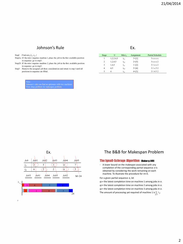
Johnson’s Rule

Note:

Johnson’s rule can find an optimum with two machines

Flow shop problem for makespan problem.

Baker p.142

.filledaresequenceinpositions

alluntil1steptoreturnandionconsideratfromjobassignedtheRemove:3Step

.3steptogo.sequencein

positionavailablefirsttheinjobtheplace,2machinerequiresmintheIf:2Step

.3steptogo.sequencein

positionavailablefirsttheinjobtheplace,1machinerequiresmintheIf:2Step

Find:1Step

tb

ta

}t,{tmin i2i1i

6

Ex.

Stage U Min tjk Assignment Partial Schedule

1 1,2,3,4,5 t31 3=[1] 3 x x x x

2 1,2,4,5 t22 2=[5] 3 x x x 2

3 1,4,5 t11 1=[2] 3 1 x x 2

4 4,5 t52 5=[4] 3 1 x 5 2

5 4 t11 4=[3] 3 1 4 5 2

7

Ex.

Job

tj1

tj2

Job1 Job2 Job3 Job4 Job5

3 5 1 6 7

6 2 2 6 5

Job3 Job1 Job4 Job5 Job2

3

1 4 5 2

2 5 4 1 3

24

M=24

8

The B&B for Makespan Problem

The Ignall-Schrage Algorithm (Baker p.149)

- A lower bound on the makespan associated with any completion of the corresponding partial sequence σ is obtained by considering the work remaining on each machine. To illustrate the procedure for m=3.

For a given partial sequence σ, let

q1= the latest completion time on machine 1 among jobs in σ.

q2= the latest completion time on machine 2 among jobs in σ.

q3= the latest completion time on machine 3 among jobs in σ.

The amount of processing yet required of machine 1 is

'j

1jt

21/04/2014

3

9

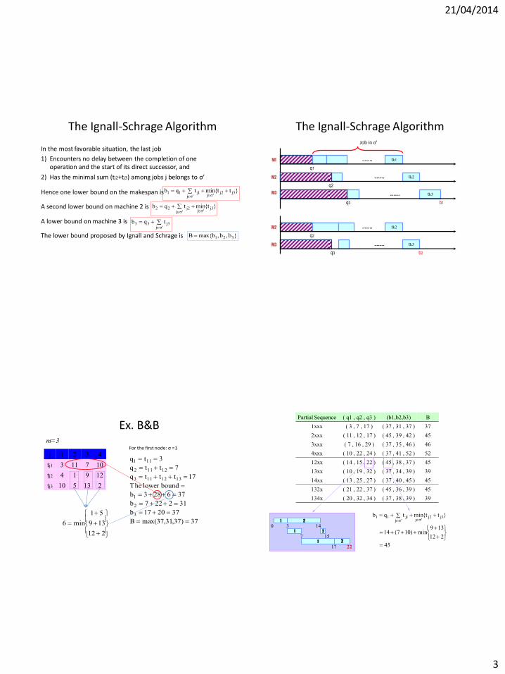
The Ignall-Schrage Algorithm

In the most favorable situation, the last job

1) Encounters no delay between the completion of one operation and the start of its direct successor, and

2) Has the minimal sum (tj2+tj3) among jobs j belongs to σ’

Hence one lower bound on the makespan is

A second lower bound on machine 2 is

A lower bound on machine 3 is

The lower bound proposed by Ignall and Schrage is

}tt{mintqb 3j2j'j'j

1j11

}t{mintqb 3j'j'j

2j22

'j

3j33 tqb

}b,b,bmax{B 321

10

The Ignall-Schrage Algorithm

M1

M2

M3

tk1

tk2

tk3

……..

……..

……..

q1

q2

q3 b1

M2

M3

tk2

tk3

……..

……..

q2

q3 b2

Job in σ’

11

Ex. B&B

j 1 2 3 4

tj1 3 11 7 10

tj2 4 1 9 12

tj3 10 5 13 2

m=3 For the first node: σ =1

37)37,31,37max(B

372017b

312227b

376283b

boundlowerThe

17tttq

7ttq

3tq

3

2

1

1312113

12112

111

212

139

51

min6

12

Ex. Partial Sequence ( q1 , q2 , q3 ) (b1,b2,b3) B

1xxx ( 3 , 7 , 17 ) ( 37 , 31 , 37 ) 37

2xxx ( 11 , 12 , 17 ) ( 45 , 39 , 42 ) 45

3xxx ( 7 , 16 , 29 ) ( 37 , 35 , 46 ) 46

4xxx ( 10 , 22 , 24 ) ( 37 , 41 , 52 ) 52

12xx ( 14 , 15 , 22 ) ( 45 , 38 , 37 ) 45

13xx ( 10 , 19 , 32 ) ( 37 , 34 , 39 ) 39

14xx ( 13 , 25 , 27 ) ( 37 , 40 , 45 ) 45

132x ( 21 , 22 , 37 ) ( 45 , 36 , 39 ) 45

134x ( 20 , 32 , 34 ) ( 37 , 38 , 39 ) 39

1 2

1 2

1 2

0 3 14

7 15

17 22 45

212

139min)107(14

}tt{mintqb 3j2j'j'j

1j11

21/04/2014

4

13

Ex. B&B

P0

1xxx 2xxx 3xxx 4xxx

B=37 B=45 B=46 B=52

12xx 13xx 14xx

B=45 B=45 B=39

132x 134x

B=45 B=39

14

Hw.

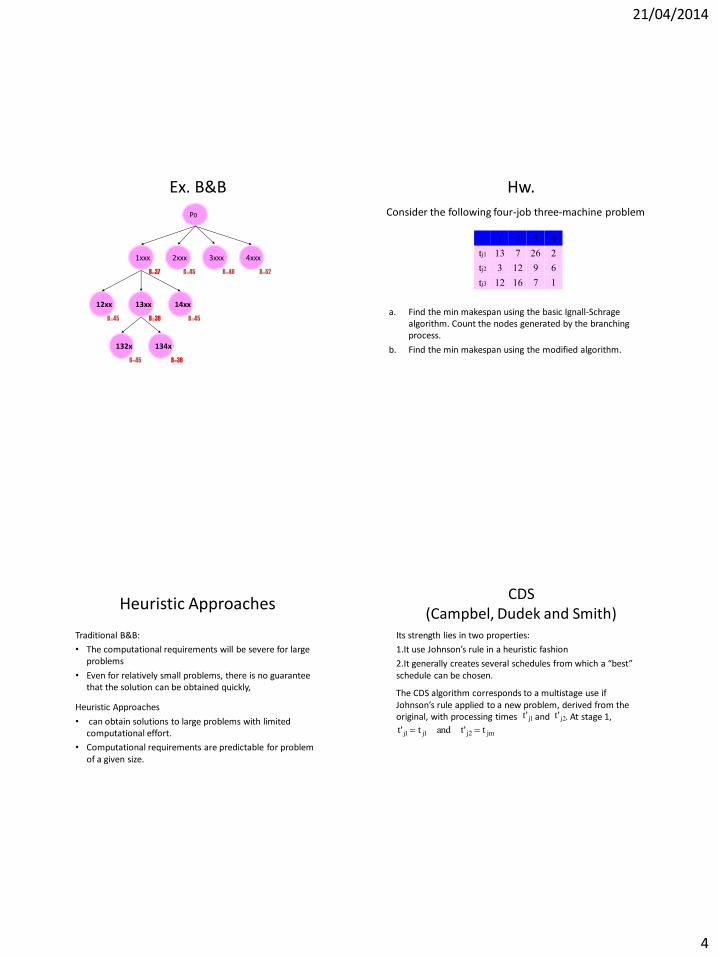
a. Find the min makespan using the basic Ignall-Schrage algorithm. Count the nodes generated by the branching process.

b. Find the min makespan using the modified algorithm.

j 1 2 3 4

tj1 13 7 26 2

tj2 3 12 9 6

tj3 12 16 7 1

Consider the following four-job three-machine problem

15

Heuristic Approaches

Traditional B&B:

• The computational requirements will be severe for large problems

• Even for relatively small problems, there is no guarantee that the solution can be obtained quickly,

Heuristic Approaches

• can obtain solutions to large problems with limited computational effort.

• Computational requirements are predictable for problem of a given size.

16

CDS (Campbel, Dudek and Smith)

Its strength lies in two properties:

1.It use Johnson’s rule in a heuristic fashion

2.It generally creates several schedules from which a “best” schedule can be chosen.

The CDS algorithm corresponds to a multistage use if Johnson’s rule applied to a new problem, derived from the original, with processing times and . At stage 1, 1j't 2j't

jm2j1j1j t'tandt't

21/04/2014

5

17

CDS

In other words, Johnson’s rule is applied to the first and mth operations and intermediate operations are ignored. At stage 2,

1m,jjm2j2j1j1j tt'tandtt't

That is, Johnson’s rule is applied to the sums of the first two and last two operation processing times. In general at stage i,

i

1k1km,j2j

i

1kjk1j t'tandt't

18

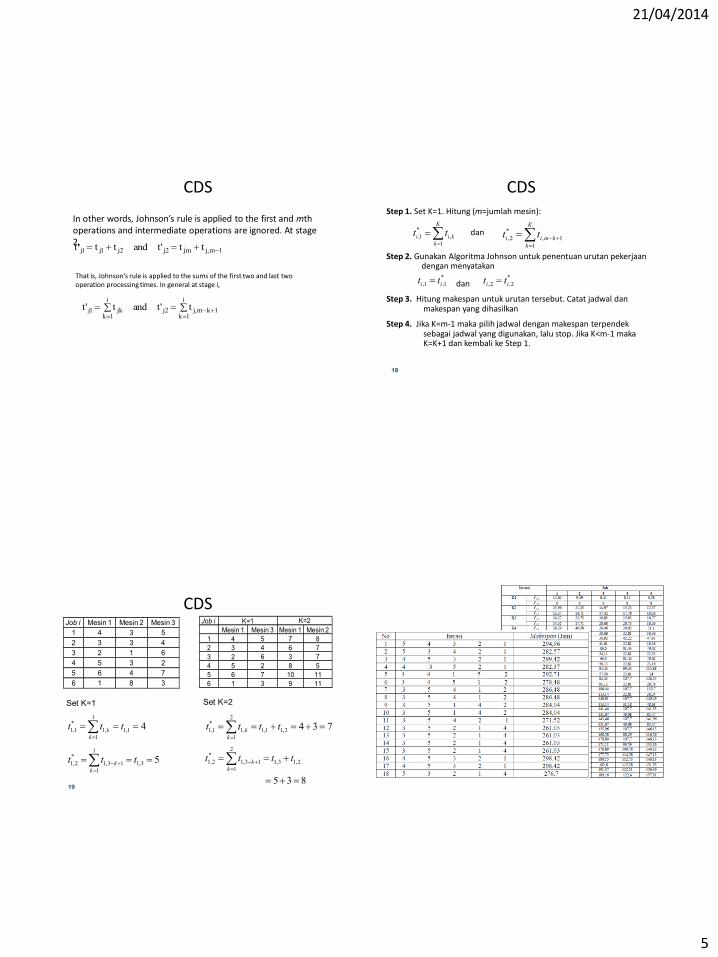
Step 1. Set K=1. Hitung (m=jumlah mesin):

dan

Step 2. Gunakan Algoritma Johnson untuk penentuan urutan pekerjaan dengan menyatakan

dan

Step 3. Hitung makespan untuk urutan tersebut. Catat jadwal dan makespan yang dihasilkan

Step 4. Jika K=m-1 maka pilih jadwal dengan makespan terpendek sebagai jadwal yang digunakan, lalu stop. Jika K<m-1 maka K=K+1 dan kembali ke Step 1.

K

k

kii tt1

,

*

1,

K

k

kmii tt1

1,

*

2,

*

1,1, ii tt *

2,2, ii tt

CDS

19

Job i

Mesin 1 Mesin 3 Mesin 1 Mesin 2

1 4 5 7 8

2 3 4 6 7

3 2 6 3 7

4 5 2 8 5

5 6 7 10 11

6 1 3 9 11

K=1 K=2Job i Mesin 1 Mesin 2 Mesin 3

1 4 3 5

2 3 3 4

3 2 1 6

4 5 3 2

5 6 4 7

6 1 8 3

Set K=1

41,1

1

1

,1

*

1,1

tttk

k

53,1

1

1

13,1

*

2,1

tttk

k

Set K=2

7342,11,1

2

1

,1

*

1,1

ttttk

k

835

2,13,1

2

1

13,1

*

2,1

ttttk

k

CDS CDS

20

21/04/2014

6

CDS

21 22

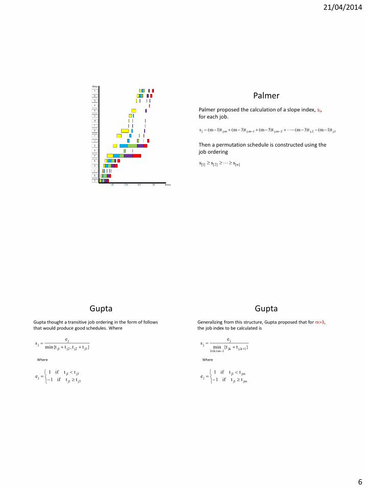
Palmer

Palmer proposed the calculation of a slope index, sj, for each job.

1,j2,j2m,j1m,jm,jj t)1m(t)3m(t)5m(t)3m(t)1m(s

Then a permutation schedule is constructed using the job ordering

]n[]2[]1[ sss

23

Gupta

Gupta thought a transitive job ordering in the form of follows that would produce good schedules. Where

}tt,ttmin{

es

3j2j2j1j

j

j

Where

3j1j

3j1j

j ttif1

ttif1e

24

Gupta

Generalizing from this structure, Gupta proposed that for m>3, the job index to be calculated is

}tt{min

es

1k,jjk1mk1

j

j

Where

jm1j

jm1j

j ttif1

ttif1e

21/04/2014

7

25

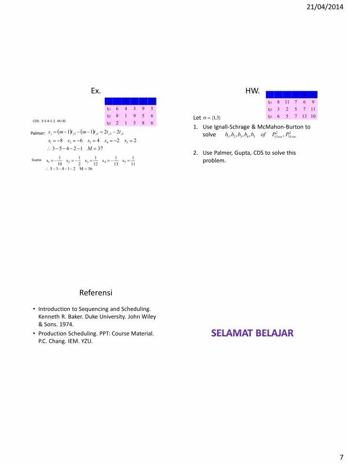
Ex.

Palmer:

j 1 2 3 4 5

tj1 6 4 3 9 5

tj2 8 1 9 5 6

tj3 2 1 5 8 6

3712453

22468

2211

54321

1313

M

sssss

tttmtms jjjjj

Gupta:

36M2143511

1s

13

1s

12

1s

2

1s

10

1s 54321

CDS: 3-5-4-1-2 M=35

26

HW.

Let

1. Use Ignall-Schrage & McMahon-Burton to solve

2. Use Palmer, Gupta, CDS to solve this problem.

j 1 2 3 4 5

tj1 8 11 7 6 9

tj2 3 2 5 7 11

tj3 6 5 7 13 10 }3,1{

2 2

1 2 3 4 5 13 31, , , , ,xxx xxxb b b b b of P P

Referensi

• Introduction to Sequencing and Scheduling. Kenneth R. Baker. Duke University. John Wiley & Sons. 1974.

• Production Scheduling. PPT: Course Material. P.C. Chang. IEM. YZU.