Flowing to the Bounce

Takeo Moroi (Tokyo)

Refs:

Chigusa, TM, Shoji, 1906.10829 [hep-ph]

PPP Workshop @ YITP, ’19.08.01

1. Introduction

The subject today: a new method to calculate the bounce

V

Φ

False vacuum

True vacuum

false vacuum decay

• False vacua show up in many particle-physics models

• Tunneling process is dominantly induced by the field con-figuration called “bounce”

Today, I try to explain

• Why is the calculation of the bounce difficult?

• What is our new idea?

• Why does it work?

• Does it really work?

Outline

1. Introduction

2. Bounce

3. Calculating Bounce with Flow Equation

4. Numerical Analysis

5. Summary

2. Bounce

Calculation of the decay rate a la Coleman

• The decay rate is related to Euclidean partition function

Z = ⟨FV|e−HT |FV⟩ ≃∫Dϕ e−S[ϕ] ∝ exp(iγV T )

• Euclidean action

S[ϕ] =∫dDx

(1

2∂µϕ∂µϕ+ V

)

• The false vacuum decay is dominated by the classical path

Z = + + + ...

= exp [ ]

one-bounceV

Φ

bouncet = -∞

t = ∞

The bounce: spherical solution of Euclidean EoM[Coleman; Callan & Coleman][

∂2ϕ− ∂V

∂ϕ

]ϕ→ϕ

=

[∂2rϕ+

D − 1

r∂rϕ− ∂V

∂ϕ

]ϕ→ϕ

= 0

with

ϕ(r = ∞) = v : false vacuum

ϕ′(0) = 0

-V

Φ

r = ∞r = 0

False Vacuum True Vacuum

False Vacuum

False Vacuum

bounce @ r=0

Bounce is important for the study of false vacuum decay

γ = Ae−S[ϕ]

Why is the calculation of ϕ so difficult?

Bounce is a saddle-point solution of the EoM

Expansion of the action around the bounce: ϕ = ϕ+Ψ

• S[ϕ+Ψ] = S[ϕ] + 1

2

∫dDxΨMΨ+O(Ψ3)

M ≡ −∂2r −

D − 1

r∂r +

∂2V

∂ϕ2

∣∣∣∣∣∣ϕ→ϕ

: fluctuation operator

• M has one negative eigenvalue (which we call λ−)[Callan & Coleman]

Fluctuation around the bounce: ϕ = ϕ+Ψ

• ∂rΨ(r = 0) = 0

• Ψ(r = ∞) = 0

We expand Ψ by using eigenfunctions of M

⇒ Mχ = λχχ

r

O R

λ = λn

λ = λn

We need to impose relevant boundary conditions

• ∂rχn(r = 0) = 0

• χn(r = ∞) = 0

An evidence of the existence of negative eigenvalue

• Functions are expanded by χn (eigenfunctions of M)

⟨χn|χm⟩ = δnm, where ⟨f |f ′⟩ ≡∫ ∞

0drrD−1f(r)f ′(r)

• f(r) =∑n⟨f |χn⟩χn(r)

• ⟨f |Mf⟩ =∑nλn⟨χn|f⟩2

Example: f(r) = r∂rϕ

• ⟨(r∂rϕ)|M(r∂rϕ)⟩ = −(D − 2)∫ ∞

0drrD−1(∂rϕ)(∂rϕ) < 0

• r∂rϕ: fluctuation w.r.t. the “scale transformation”

ϕ((1 + ϵ)r) ≃ ϕ(r) + ϵ r∂rϕ+ · · ·

Undershoot-overshoot method to calculate the bounce

∂2rϕ+

D − 1

r∂rϕ− ∂V

∂ϕ= 0

2nd term is a “friction,” which disappears as r → ∞

There should exist bounce, satisfying ϕ′(0) = 0 and ϕ(∞) = v

• If ϕ(0)<∼ vc

⇒ Undershoot

• If ϕ(0) ≃ vT

⇒ Overshoot

• There exists right ϕ(0)

⇒ ϕ(∞) = v

-V

φ

v vT

vc

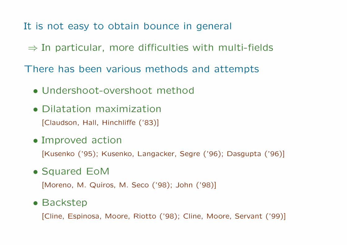
It is not easy to obtain bounce in general

⇒ In particular, more difficulties with multi-fields

There has been various methods and attempts

• Undershoot-overshoot method

• Dilatation maximization[Claudson, Hall, Hinchliffe (’83)]

• Improved action[Kusenko (’95); Kusenko, Langacker, Segre (’96); Dasgupta (’96)]

• Squared EoM[Moreno, M. Quiros, M. Seco (’98); John (’98)]

• Backstep[Cline, Espinosa, Moore, Riotto (’98); Cline, Moore, Servant (’99)]

• Improved potential[Konstandin, Huber (’06); Park (’10)]

• Path deformation[Wainwright (’11)]

• Perturbative method[Akula, Balazs, White (’16); Athron et al. (’19)]

• Multiple shooting[Masoumi, Olum, Shlaer (’16)]

• Tunneling potential[Espinosa (’18); Espinosa, Konstandin (’18)]

• Polygon approximation[Guada, Maiezza, Nemevsek (’18)]

• Machine learning[Jinno (’18); Piscopo, Spannowsky, Waite (’19)]

3. Bounce from Flow Equation

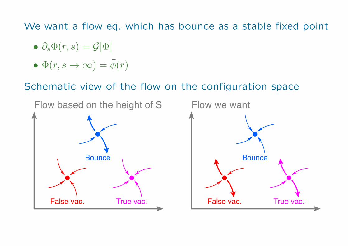
We want a flow eq. which has bounce as a stable fixed point

• ∂sΦ(r, s) = G[Φ]

• Φ(r, s → ∞) = ϕ(r)

Schematic view of the flow on the configuration space

Flow based on the height of S

False vac. True vac.

Bounce

Flow we want

False vac. True vac.

Bounce

Flow based on the height of S

∂sΦ(r, s) = F (r, s)

F ≡ −δS[Φ]δΦ

= ∂2rΦ +

D − 1

r∂rΦ− ∂V (Φ)

∂Φ

Behavior of fluctuations around the bounce

Φ(r, s) = ϕ(r) +∑nan(s)χn(r)

⇒∑nanχn ≃ −M

∑nanχn = −

∑nλnanχn

⇒ an ≃ −λnan

Because of χ−, bounce cannot be a stable fixed point

⇒ This does not work

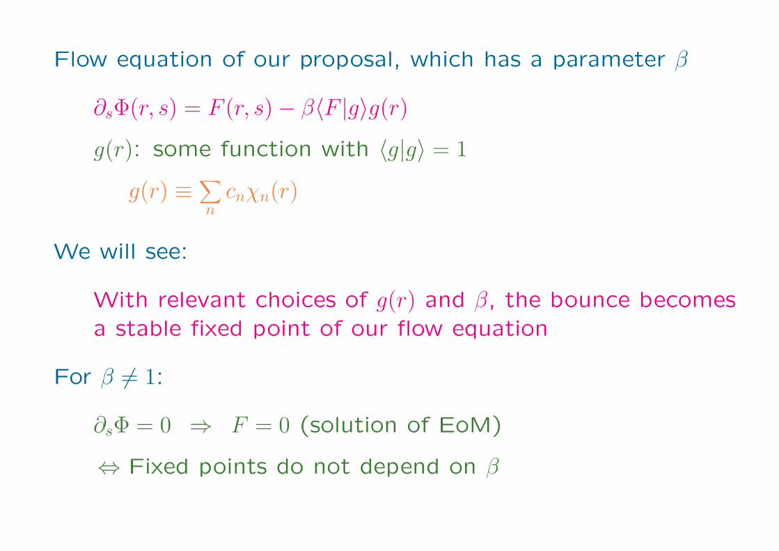
Flow equation of our proposal, which has a parameter β

∂sΦ(r, s) = F (r, s)− β⟨F |g⟩g(r)

g(r): some function with ⟨g|g⟩ = 1

g(r) ≡∑ncnχn(r)

We will see:

With relevant choices of g(r) and β, the bounce becomesa stable fixed point of our flow equation

For β = 1:

∂sΦ = 0 ⇒ F = 0 (solution of EoM)

⇔ Fixed points do not depend on β

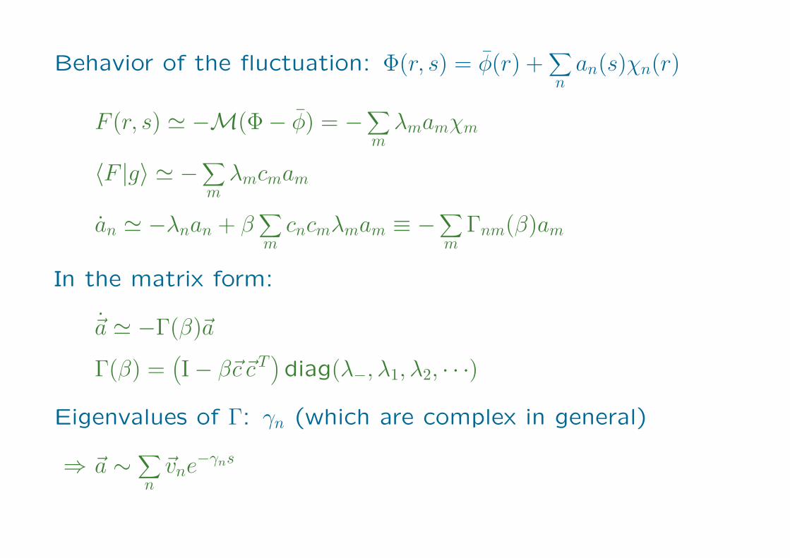
Behavior of the fluctuation: Φ(r, s) = ϕ(r) +∑nan(s)χn(r)

F (r, s) ≃ −M(Φ− ϕ) = −∑mλmamχm

⟨F |g⟩ ≃ −∑mλmcmam

an ≃ −λnan + β∑mcncmλmam ≡ −

∑mΓnm(β)am

In the matrix form:

˙a ≃ −Γ(β)a

Γ(β) =(I− βc cT

)diag(λ−, λ1, λ2, · · ·)

Eigenvalues of Γ: γn (which are complex in general)

⇒ a ∼∑nvne

−γns

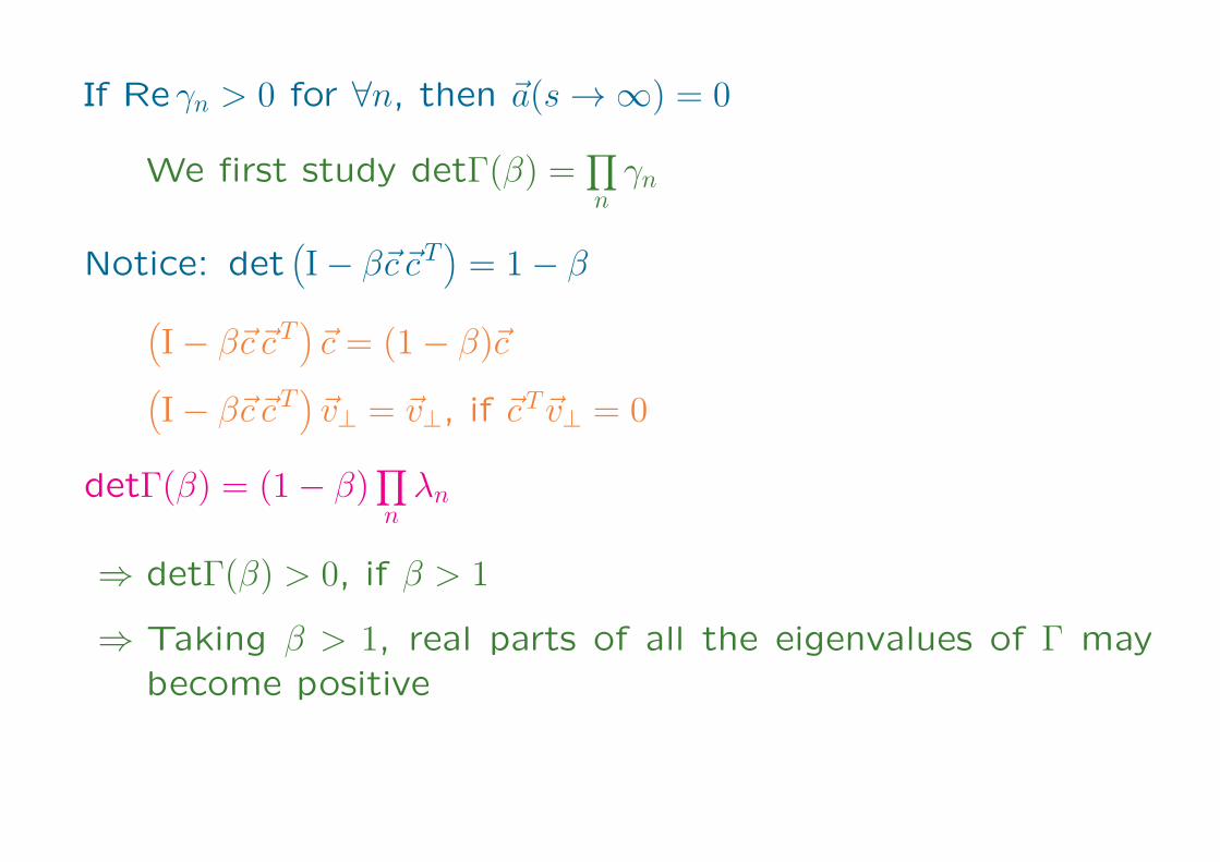
If Re γn > 0 for ∀n, then a(s → ∞) = 0

We first study detΓ(β) =∏nγn

Notice: det(I− βc cT

)= 1− β

(I− βc cT

)c = (1− β)c(

I− βc cT)v⊥ = v⊥, if cT v⊥ = 0

detΓ(β) = (1− β)∏nλn

⇒ detΓ(β) > 0, if β > 1

⇒ Taking β > 1, real parts of all the eigenvalues of Γ maybecome positive

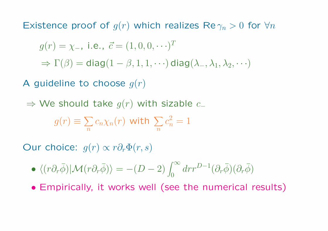
Existence proof of g(r) which realizes Re γn > 0 for ∀n

g(r) = χ−, i.e., c = (1, 0, 0, · · ·)T

⇒ Γ(β) = diag(1− β, 1, 1, · · ·)diag(λ−, λ1, λ2, · · ·)

A guideline to choose g(r)

⇒ We should take g(r) with sizable c−

g(r) ≡∑ncnχn(r) with

∑nc2n = 1

Our choice: g(r) ∝ r∂rΦ(r, s)

• ⟨(r∂rϕ)|M(r∂rϕ)⟩ = −(D − 2)∫ ∞

0drrD−1(∂rϕ)(∂rϕ)

• Empirically, it works well (see the numerical results)

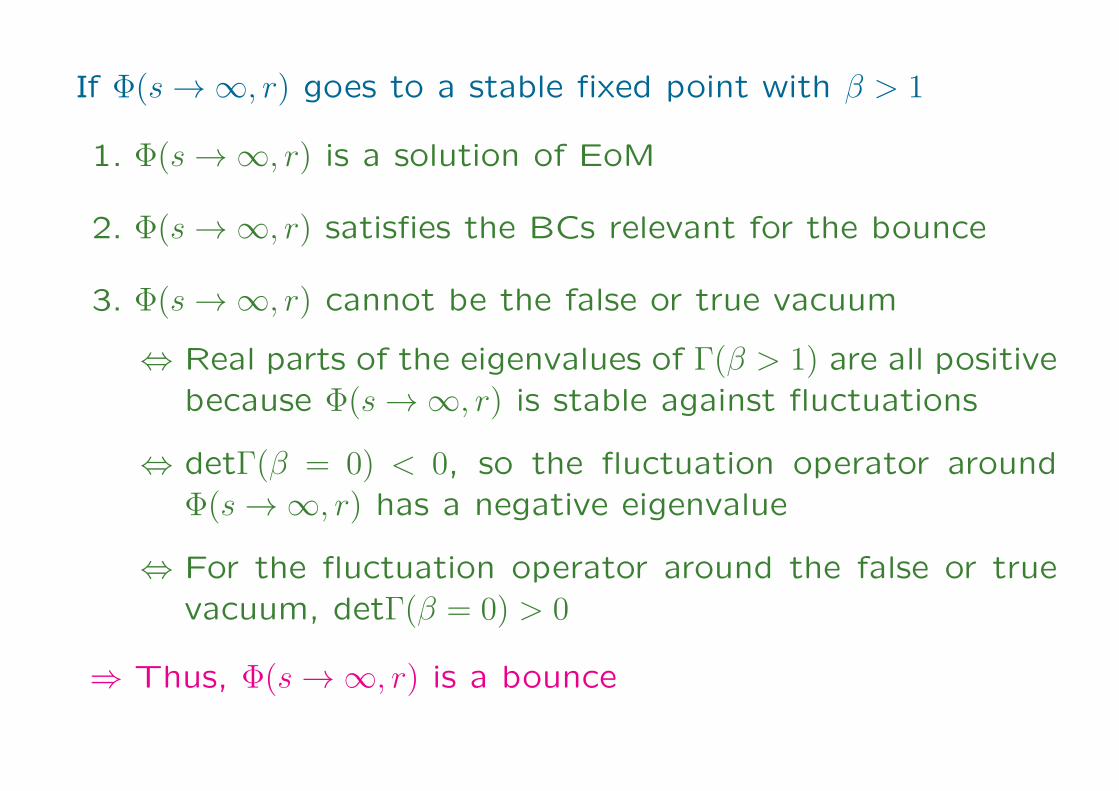
If Φ(s → ∞, r) goes to a stable fixed point with β > 1

1. Φ(s → ∞, r) is a solution of EoM

2. Φ(s → ∞, r) satisfies the BCs relevant for the bounce

3. Φ(s → ∞, r) cannot be the false or true vacuum

⇔ Real parts of the eigenvalues of Γ(β > 1) are all positivebecause Φ(s → ∞, r) is stable against fluctuations

⇔ detΓ(β = 0) < 0, so the fluctuation operator aroundΦ(s → ∞, r) has a negative eigenvalue

⇔ For the fluctuation operator around the false or truevacuum, detΓ(β = 0) > 0

⇒ Thus, Φ(s → ∞, r) is a bounce

4. Numerical Analysis

We considered single- and double scalar cases:

• Single-scalar case:

V (1) =1

4ϕ4 − k1 + 1

3ϕ3 +

k12ϕ2

– False vacuum: ϕ = 0

– True vacuum: ϕ = 1

• Double-scalar case:

V (2) =(ϕ2x + 5ϕ2

y

) [5(ϕx − 1)2 + (ϕy − 1)2

]+ k2

(1

4ϕ4y −

1

3ϕ3y

)

– False vacuum: (ϕx, ϕy) = (0, 0)

– True vacuum: (ϕx, ϕy) = (1, 1)

• We compare our results with those of CosmoTransitions

[Wainwright]

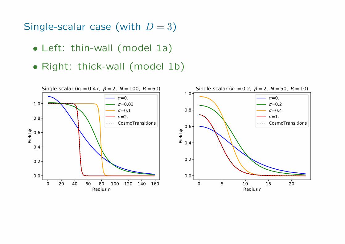
Single-scalar case (with D = 3)

• Left: thin-wall (model 1a)

• Right: thick-wall (model 1b)

Double-scalar case (with D = 3)

• Left: thin-wall (model 2a)

• Right: thick-wall (model 2b)

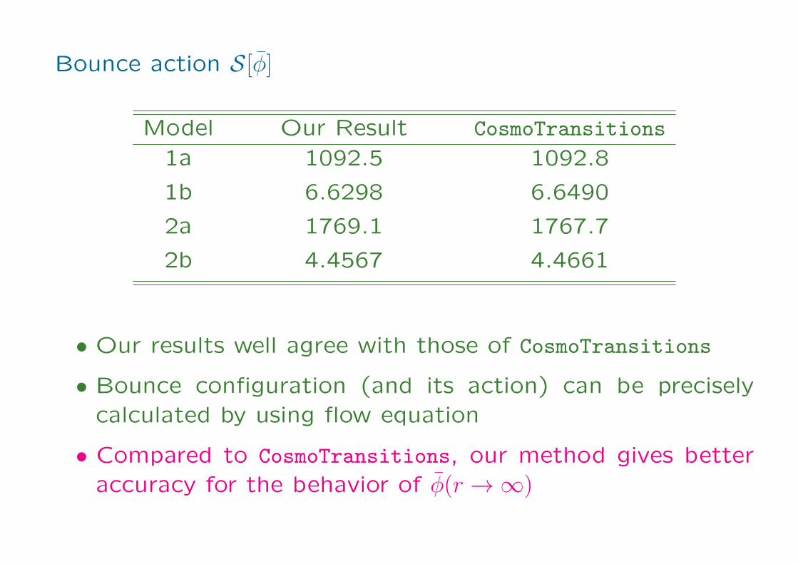
Bounce action S[ϕ]

Model Our Result CosmoTransitions

1a 1092.5 1092.8

1b 6.6298 6.6490

2a 1769.1 1767.7

2b 4.4567 4.4661

• Our results well agree with those of CosmoTransitions

• Bounce configuration (and its action) can be preciselycalculated by using flow equation

• Compared to CosmoTransitions, our method gives betteraccuracy for the behavior of ϕ(r → ∞)

Another approach[Coleman, Glaser, Martin (’78); Sato (’19)]

1. Determine the configuration φ(r;P) which minimizes S onthe hypersurface with constant P

P ≡∫dDxV

Flow equation:

∂sΦ(r, s) = F − ξ[Φ]∂V

∂Φ

At the fixed point: φ(r;P) = Φ(r, s → ∞)

∂2r φ+

D − 1

r∂rφ− λ2∂V

∂φ= 0

λ2 = ξ[Φ(s → ∞)] + 1

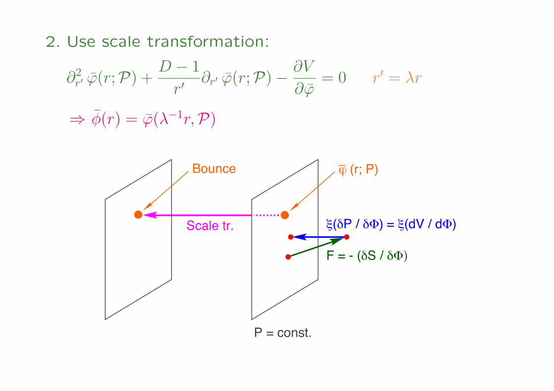
2. Use scale transformation:

∂2r′ φ(r;P) +

D − 1

r′∂r′ φ(r;P)− ∂V

∂φ= 0 r′ = λr

⇒ ϕ(r) = φ(λ−1r,P)

Scale tr.

F = - (δS / δΦ)

ξ(δP / δΦ) = ξ(dV / dΦ)

ϕ (r; P)

P = const.

_Bounce

5. Summary

We proposed a new method to calculate the bounce

• Our method is based on the gradient flow

• The bounce is obtained by solving the flow equation

• It can be easily implemented into numerical code

To-do list:

• Application to BSM models (in particular, SUSY)[Gunion, Haber, Sher; Casas, Lleyda, Munoz; Kusenko, Langacker, Segre;

Camargo-Molina et al.; Chowdhury et al.; Blinov and Morrissey; Endo, Mo-

roi, Nojiri; Endo, Moroi, Nojiri, Shoji; · · ·]

• Making a public code (?)

Please use our method, if you find any good application