CHAPTER NO. FULLY NONLINEAR POTENTIAL FLOW MODELS USED FOR LONG WAVE RUNUP PREDICTION (S. Grilli, Department of Ocean Engineering, University of Rhode Island, Kingston 02881, RI) Abstract A review of Boundary Integral Equation methods used for long wave runup prediction is presented in this chapter. In Section 1, a brief literature review is given of methods used for modeling long wave propagation and of generic methods and models used for modeling highly nonlinear waves. In Section 2, fully nonlinear potential flow equations are given for the Boundary Element Model developed by the author, including boundary conditions for both wave generation and absorption in the model. In Section 3, details are given for the generation of waves in the model using various methods (wavemakers, free surface potential, internal sources). In Section 4, the numerical implementation of the author’s model based on a higher-order Boundary Element Method is briefly presented. In Section 5, many applications of the model are given for the computation of wave propagation, shoaling, breaking or runup on slopes, and interaction with submerged and emerged structures. The last application presented in this Section is the Benchmark #3 problem for the runup of solitary waves on a vertical wall that was proposed as part of the “International Workshop on Long-wave Runup Models (San Juan Island, WA, USA, 09/95). Finally, Appendices A to F give more details about various aspects of the numerical model. 1. Introduction 1.1. Modeling of long wave propagation, shoaling, breaking and runup Over the past forty years, ocean wave propagation, shoaling, breaking or runup over a slope, have been the object of numerous theoretical and numerical studies, particularly for the case of—essentially two-dimensional—long waves or swells generated by wind (wind waves) or earthquakes (tsunamis). Main approaches pursued were based on using : (i) linear or nonlinear Shallow Water Wave equations (Carrier and Greenspan 8 1958, Carrier 7 1966, Camfield and Street 6 1969, Hibberd and Peregrine 50 1979, Kobayashi et al. 57 1989, and Synolakis 89 1990); (ii) Boussinesq or parabolic approximations of Boussinesq equations (Peregrine 72 1967, Pedersen and Gjevik 71 1983, Freilich and Guza 24 1984, Zelt and Raichlen 97 1990, and
Transcript
CHAPTER NO.
FULLY NONLINEAR POTENTIAL FLOW MODELSUSED FOR LONG WAVE RUNUP PREDICTION
(S. Grilli, Department of Ocean Engineering, University of Rhode Island, Kingston 02881, RI)
AbstractA review of Boundary Integral Equation methods used for long wave runup prediction
is presented in this chapter.In Section 1, a brief literature review is given of methods used for modeling long wave
propagation and of generic methods and models used for modeling highly nonlinear waves.In Section 2, fully nonlinear potential flow equations are given for the Boundary ElementModel developed by the author, including boundary conditions for both wave generationand absorption in the model. In Section 3, details are given for the generation of wavesin the model using various methods (wavemakers, free surface potential, internal sources).In Section 4, the numerical implementation of the author’s model based on a higher-orderBoundary Element Method is briefly presented. In Section 5, many applications of themodel are given for the computation of wave propagation, shoaling, breaking or runupon slopes, and interaction with submerged and emerged structures. The last applicationpresented in this Section is the Benchmark #3 problem for the runup of solitary waves ona vertical wall that was proposed as part of the “International Workshop on Long-waveRunup Models (San Juan Island, WA, USA, 09/95). Finally, Appendices A to F give moredetails about various aspects of the numerical model.
1. Introduction
1.1. Modeling of long wave propagation, shoaling, breaking and runup
Over the past forty years, ocean wave propagation, shoaling, breaking or runup over aslope, have been the object of numerous theoretical and numerical studies, particularly forthe case of—essentially two-dimensional—long waves or swells generated by wind (windwaves) or earthquakes (tsunamis).
Main approaches pursued were based on using : (i) linear or nonlinear Shallow WaterWave equations (Carrier and Greenspan 8 1958, Carrier 7 1966, Camfield and Street 6
1969, Hibberd and Peregrine 50 1979, Kobayashi et al. 57 1989, and Synolakis 89 1990);(ii) Boussinesq or parabolic approximations of Boussinesq equations (Peregrine 72 1967,Pedersen and Gjevik 71 1983, Freilich and Guza 24 1984, Zelt and Raichlen 97 1990, and
Kirby 55 1991) a. Most of the methods used in these works, however, are based on first-or low-order theories whose assumptions—for instance small amplitude, mildly nonlinearwaves, or mild bottom slope—may no longer be valid for waves that, due to shoaling, maybe close to breaking at the top of a slope (i.e., strongly nonlinear) before they run-up orbreak on the slope.
Until recently, state-of-the-art methods used for predicting characteristics of highlynonlinear waves shoaling over a sloping bottom up to impending breaking (e.g., shoalingcoefficients, breaker height and kinematics), were based on higher-orderexpansion methodsoriginally developed for waves of permanent form over constant depth (Stiassine andPeregrine 84 1980, Peregrine 73 1983, Sobey and Bando 82 1991). These methods, however,by nature cannot include effects of finite bottom slope or changes of wave form duringshoaling. Long waves, in particular, are known to become strongly asymmetric whenshoaling over a gentle slope and approaching breaking (e.g., experiments by Skjelbreia 78
1987, Grilli et al.41 1994), an effect that is not included in the above approaches. Griffithset al. 28 1992, compared measurements of internal kinematics of periodic waves shoalingup a 1:30 slope with predictions of the 5th-order Stokes theory, the 9th- and higher-orderstreamfunction theory, and the full nonlinear model by New et al. 65. They found thathorizontal velocities were correctly predicted by most theories below still water level but b
, in the high crest region, low-order theories underpredicted velocities by as much as 50%whereas predictions of the fully nonlinear theory were quite good up to the crest c. Grilliet al.41 1994 showed that computations with a fully nonlinear potential model quite wellpredicted the shape of solitary waves during shoaling over a 1:35 slope, as measured inwell-controlled laboratory experiments. The agreement was within 2%, both in time andspace, up to the breaking point. The same computations also showed that, even for longwaves, horizontal velocities under a shoaling wave crest eventually become significantlynon-uniform over depth (in some cases by more than 200%), an effect which is neglectedin (first-order) nonlinear shallow water wave theories.
Grilli et al.40 1994 and Wei et al.93 1995 recently compared predictions of classical(i.e., weakly nonlinear and weakly dispersive) and modified (i.e., with improved dispersioncharacteristics and/or full nonlinearity) Boussinesq models (BM) to the full nonlinearpotential flow solution—used as a reference—for the shoaling of solitary waves over slopes1:100 to 1:8, up to the breaking point. They found that, in the region of large nonlinearitywhere the ratio wave height over depth is larger than 0.5, the classical BM significantlyoverpredicts crest height and particle velocity. This model also predicts spurious secondarytroughs behind the main crest. The fully nonlinear BM, however, was found much moreaccurate in predicting both wave shape and horizontal velocity under the crests, from bottomto surface. Similar conclusions were reached for the propagation of highly nonlinear undularbores over constant depth.
aThe reader can find details on various wave theories and summaries of some of the above referenced worksin Mei 63 1983, and Dean and Dalrymple 17 1984.bsee Ref.17 for definitions of these wave theories.cNote that these comparisons were only done for a mild slope (i.e, with limited bottom effect) and for casesin which breaking occurred by spilling. The authors pointed out that “all theories are grossly in error whencompared to severe plunging breakers”.
- 0 .3-0 .2-0 .1
0.00.10.20.3
0 0.5 1 1.5 2
η/ h
x / h
Fig Instability by plunging breaking of a large sine wave over constant depth h as computedwith the model by Grilli et al. 36 Initial wave height is Hh 0333 length Lh 185and period T
pgL 250 A periodicity condition is used in the model on lateral boundaries to
create a situation similar to that examined by LonguetHiggins and Cokelet 62 Symbols denoteBEM discretization nodes identical to individual uid particles whose motion is calculated in time
In the above studies, it is thus seen that a correct representation of both the shapeand kinematics of strongly nonlinear long waves can only be achieved when using highlyor fully nonlinear models, i.e., models in which no approximation are introduced for thefree surface boundary conditions. Even for long waves with very small nonlinearity whenapproaching the deep water end of a slope, it is also seen that long distances of propagationover a gentle slope can make such waves both strongly asymmetric and nonlinear towardsthe top of the slope, whether they subsequently break or simply run up the slope.
These conclusions justify using fully nonlinear models for studying shoaling, runup orbreaking, of large long waves close to the shore.
1.2. Modeling of highly nonlinear waves
Over the past twenty years, considerable efforts have been devoted to developingincreasingly accurate and efficient models for fully nonlinear water waves at sea. Startingwith the key work by Longuet-Higgins and Cokelet62 1976, the most successful approachesso far have been based on describing the physical problem based on potential flow theory(i.e., neglecting both viscous and rotational effects on the wave flow) while keeping fullnonlinearity in the free surface boundary conditions (i.e., a “Fully Nonlinear PotentialFlow” (FNPF) model). Most methods have also used a representation of the flow thatallows for multi-valued free surface elevations appearing during breaking (i.e., a mixedEulerian-Lagrangian representation; see Fig. 1). Despite its intrinsic limitations, potentialflow theory has been shown in many applications to model the physics of wave propagationand overturning in deep water, and wave shoaling up to breaking or runup over slopes, witha surprising degree of accuracy (e.g., Dommermuth et al.20, Grilli30, and Grilli et al.414748;see below for a discussion).
Many quite exhaustive reviews of the relevant literature have been published to dateand can be consulted for more information (e.g., Grilli30, Grilli et al.3638, Peregrine7374,Yeung95). For the purpose of introducing the present numerical model and its applicationsto long wave propagation and runup, the following is a brief description of the main steps in
- 1 .5
- 1
-0 .5
0
0.5
0 5 1 0 1 5 2 0 2 5 3 0 3 5 4 0 4 5 5 0
ho
h1
xl
xl+ l
x / ho
z / ho
AB
1:35
Fig Generation and shoaling over a slope of numerically exact periodic waves streamfunction
waves with initial height Hoho 01 and period Tpgho 355 as computed by Grilli and
Horrillo 31 To achieve zeromassux and thus constant volume in the computational domain wavesare generated on top of an opposite current equal to the mean mass transport velocity An absorbingbeach AB of length l with counteracting free surface pressure is speci ed for xl 38 over a shelfof depth h1 005
the development of FNPF models that will identify key elements of the problem. Startingwith Longuet-Higgins and Cokelet 62, the problem was first formulated in deep water byassuming that waves were two-dimensional in the vertical plane—i.e., long crested—andperiodic in space, thus making it possible to use conformal mapping techniques whichwrap the computational domain on itself and eliminate the need for lateral boundaries inthe model. Doing so, deep water plunging breakers could be calculated up to touch downof the jet on the free surface (Fig. 1). Along this line, various increasingly accurate andstable numerical formulations were proposed for both deep and constant water depth, andapplications sometimes also included periodic structures (Dold and Peregrine 18, New etal.65, and Vinje and Brevig 92) d. Results of such computations were compared to laboratorymeasurements and found to agree with them up to the latest stages of wave breaking, thusconfirming the validity of the FNPF approach to model the physics of wave breaking farfrom the shore (e.g., Dommermuth et al. 20).
Most of the previous and similar models—except perhaps the improvement of Doldand Peregrine’s model by Cooker13 and Cooker et al.15—due to their intrinsic nature, wereunable or had the greatest difficulties generating and propagating waves over complexbottom topography. This, however, is required for solving problems of wave shoaling andbreaking in shallow water and over beaches, and problems of wave interaction with coastalstructures and runup on slopes. To solve such problems, models working in the so-calledphysical space must be used which brings additional problems of wave generation and/orwave absorption in the computational domain and of treatment and representation of cornersin the modeled boundary (these aspects are discussed in individual Sections below). Earlyworks that addressed problems of wave generation by a wavemaker in the physical spaceare the model by Kim et al.54 which, however, was limited to non-breaking (single-valueelevation) waves, and the model by Lin et al.60, who used and improved Vinje and Brevig’sformulation but somewhat restricted their scope of application. More recent models working
dAlso note the somewhat different method introduced by Zaroodny and Greenberg 96, and Baker et al.5, basedon a vortex sheet approach.
in the physical space can accommodate almost arbitrary incident waves, complex bottomtopography, and moving boundaries (e.g., Cointe10, Grilli et al.3639, Klopman56, Ohyamaand Nadaoka67). An example of such recent computations for the shoaling and absorptionof periodic waves over a gentle slope is given in Fig. 2.
In most FNPF applications to date, the governing (Laplace’s) equation is solved usinga higher-order Boundary Element Method (BEM), either based on Green’s identity or onCauchy integral theorem formulations, and on time integrating the free surface boundarycondition using either a time marching predictor-corrector method 6292 (Runge-Kutta and/orAdams-Bashforth-Moulton schemes) or a Taylor series expansion method1836. The FNPFmodel by Grilli et al.363946, which will be used in the present applications, was developed inthe physical space following the strategy of deep water and constant depth nonlinear wavemodels mentioned above (e.g., Dold and Peregrine 18). It is based on a mixed Eulerian-Lagrangian representation with full nonlinearity in the free surface boundary conditions.FNPF equations are solved by a BEM based on Green’s identity, which easily accounts forarbitrary bottom topography and almost arbitrary incident wave conditions. Developmentof this model was carried out under a 2D formulation, which makes the model directlyapplicable to shoaling and breaking and/or runup over arbitrary slopes of normally incidentlong crested waves, without any approximation on the wave shape or on the free surfaceboundary conditions e. Many validations (both analytical and experimental) of Grilli etal.’s model and of its more recent improved versions were carried out, mostly using solitarywaves, for : (i) shallow water wave generation, propagation, and reflection, by Grilli andSvendsen4547; (ii) wave runup over a steep slope, by Svendsen and Grilli87; (iii) shoalingand breaking over both gentle and steep slopes, by Grilli et al.4148; (iv) wave impact on amixed breakwater, by Grilli et al.3335; and (v) wave propagation over a submerged obstacle,by Grilli et al.3234.
For completeness, other fully nonlinear wave models used for calculating wave prop-agation and runup on slopes (most of them based on boundary integral formulations) willbe mentioned. These models have either inherently been limited to non-breaking waves(Fenton and Rienecker 23 1982, Nakayama 64 1983, Liu et al.61 1992) or have repre-sented extensions (e.g., to axisymmetric problems) or variant of existing methods—mostlyby186292—(Isaacson 51 1982, Jansen 53 1986, Dommermuth and Yue 19 1987, Gravert 26
1987, Greenhow 27 1987, Tanaka et al. 91 1987, Romate 76 1990, Seo and Dalrymple 77
1990).Detailed equations and numerical procedures for Grilli et al.’s wave model are presented
in Sections 2,3, and 4, and applications of the model to cases of long wave propagation inshallow water and runup on slopes are presented in Section 5.
eNote that all elements in Grilli et al.’s model were selected to allow implementation of a three-dimensionalmodel as a direct extension of the 2D formulation. This is unlike 2D FNPF models based on complex variableformulations. Such extensions of FNPF models in the physical space to three-dimensional problems havealready been proposed by Romate 7576 1990, Yue94 1992, and Broeze3 1993, but still face challenges posedby the formidable size of the computational problem as well as problems of both representation of the freesurface and boundary conditions at intersections between side walls and the free surface.
2. Mathematical model
Governing equations for the two-dimensional FNPF model by Grilli et al. 3646 and itsmost recent extensions are presented in the next subsections. Full nonlinearity is maintainedin the free surface boundary conditions, and time integration of these conditions is basedon higher-order Taylor expansions, for both the free surface position and the potential.No-flow boundary conditions are prescribed along solid boundaries of the domain (bottom,coastal structures) and arbitrary waves are generated in the model, either by specifying aninitial wave on the free surface, either by simulating a wavemaker at the open-sea boundaryof the computational domain (as in laboratory experiments), or by using a line of internalsources. Finally, wave energy absorption can be specified in the model using an absorbingbeach.
2.1. Governing equations and solid boundary conditions
The velocity potential x t is used to describe inviscid irrotational 2D flows in thevertical plane x z, where the velocity is given by u r uw. Continuity equationin the fluid domain t, with boundary t, is a Laplace’s equation for the potential (seeFig. 3 for definitions),
r2 0 in t (1)
On the free surface f t, satisfies the nonlinear kinematic and dynamic boundaryconditions,
Dr
Dt u r on f t (2)
D
Dt gz 1
2r r pa
on f t (3)
respectively, with r the position vector of a free surface fluid particle, g the accelerationdue to gravity, z the vertical coordinate (positive upwards, and z 0 at the undisturbedfree surface), pa the atmospheric pressure, and the fluid density. The material derivativeis defined as,
D
Dt
t u r (4)
Along the stationary bottom b and other fixed boundaries denoted as r2, a no-flowcondition is prescribed as,
r n
n 0 on b and r2 (5)
in which n is the unit outward normal vector.
2.2. Boundary conditions for wave generation
- 2
- 1
0
1
0 1 0 2 0 3 0 4 0 5 0 6 0 7 0
Γb
x / ho
z / ho
ho h
1s
Γf( t )
Γr1
( t ) Ω ( t )Γ
r2
ns
Fig Typical computational domain for wave shoaling over a slope with de nition of variousboundaries The domain has a slope s terminated by a shelf of depth h1 at its upper part casewhere waves break before reaching the top of the slope The sketched free surface pro le corresponds
to a cnoidal wave of initial height Hoho 02 and period Tpgho 25 generated by a piston
wavemaker on boundary r1t
In models developed in the physical space, it is necessary to generate waves at oneextremity of the computational domain. Kim et al.54, Lin et al.60, Cointe10, Dommermuthet al.1920, and Grilli et al.36 generated waves in their FNPF models using surface-piercingnumerical wavemakers. Brorsen and Larsen4 proposed a different approach for generatingwaves using internal sources, which was also used by Grilli and Svendsen43 and Ohyamaand Nadaoka66 in their models.
When using a wavemaker to generate waves, there is a corner in the model, at theintersection between the wavemaker and the free surface, separating boundary segmentswith both different boundary conditions and normal directions. Possible singularity of theflow near such an intersection has given rise to substantial concern in the literature. Grilli andSvendsen46 reviewed such singularity problems and showed that, in the particular contextof wavemakers starting from a state of rest (“cold start”), provided the initial accelerationof the wavemaker is small with respect to gravity and corner boundary conditions are well-posed in the model, numerically speaking, there will be no strong singularity at the freesurface corner (at least in the FNPF regime). Thus, in the applications, they used an initialdamping function for the wavemaker motion in such a way that the acceleration remain smallduring the first few time steps of the computations. They also ensured well-posedness ofgoverning equations and boundary conditions on both sides of corners using a double-noderepresentation combined with (continuity and compatibility) conditions expressing thatpotential and velocity are unique at corners (see Grilli and Svendsen46 for more details).Many validations of Grilli and Svendsen’s model were conducted for numerical piston orflap type wavemakers, particularly with solitary waves (e.g., Grilli et al.33343641454647).Extensions of compatibility relationships that further improve numerical accuracy at cornerswere proposed by Otta et al.70 and Svendsen et al.88, and their application and validationfor the wavemaking problem was further discussed by Grilli and Subramanya39.
Assuming “numerically well-posed” wavemaker boundary conditions, it is well known,however, that a clean finite amplitude wave cannot be generated using solid wavemakers,whether in laboratory tanks or in nonlinear wave models (see, e.g., Mei63 p. 578). Essen-
tially, due to wave nonlinearity, higher-order harmonics are being generated that modulatethe shape of the wave one intends to generate. This is because sinusoidal waves or otherfirst-order solutions like Boussinesq solitary waves are not exact solutions of the fully non-linear problem. To overcome this difficulty and generate “clean” finite amplitude wavesin their model, Grilli and Svendsen46 used the numerically exact method by Tanaka90 togenerate solitary waves, and Klopman56, Subramanya and Grilli85, and Grilli and Horrillo31
used the exact periodic wave solution of the FNPF problem (i.e., a streamfunction wave(SFW) solution; Dean and Dalrymple17 p. 305) to generate periodic waves f.
In the present model,waves are thus generated either by prescribing a wavemaker motionon the “open sea” boundary r1t of the computational domain, either by prescribing theelevation and potential on the free surface of a known “exact” wave solution of flowequations, or by using an internal line of sources.
General boundary conditions for these three types of wave generation are given in thefollowing. Generation of specific waves is discussed in Section 3.
2.2.1. Plane wavemaker
A plane wavemaker motion x xpz t can be specified on the moving boundaryr1t to generate waves as in laboratory experiments. In this case, normal velocity isspecified over the surface of the paddle as,
n up n
xp
tq1 xp
z2
on r1t (6)
in which the right hand side represents the normal paddle velocity. Eq. (6) is developed inSection 3 for the case of piston or flap wavemakers.
2.2.2. Exact wave solutions
“Numerically exact” permanent form solutions of the FNPF boundary value problemover constant depth (eqs. (1)-(5); i.e., solitary or streamfunction waves) can be generatedeither by specifying their potential x to and elevation x to on the free surface f toat initial time to (solitary waves), or by specifying their horizontal velocity and accelerationuz ut along a vertical wavemaker boundary (streamfunction waves).
For exact solitary waves, normal velocity is also prescribed to Ut over the fixedvertical lateral boundaries r1, r2. We thus get,
x to z x to on f to
n Ut on r1, r2 (7)
in which overbars denote prescribed values.
fNote that SFW’s were also used in periodic FNPF models by Skourup et al.80 and Grilli et al.36.
Streamfunction waves, unlike linear periodic waves, have a non-zero horizontal massflux. When specified at one extremity of the model, such waves thus lead to a continuousaccumulation of water in the computational domain. In Klopman’s56 computations, onlysteep slopes were modeled in fairly short computational domains and waves were computedover a few periods only. Hence, water accumulation was small and did not cause anyapparent problem. In Subramanya and Grilli’s85 shoaling computations, however, with alonger computational domain and for a larger number of wave periods, water accumulationresulted in a significant increase in the mean water level that clearly affected wave shape.For the corresponding coastal problem, one would expect an offshore return flow to occurunder wave troughs (undertow) and cancel the incoming wave mass flux at some distancefrom the shore, thereby ensuring constant water volume in the nearshore region. Hence,water accumulation in the computational domain is non-physical and should be prevented.Grilli and Horrillo31 1995 proposed a method for achieving zero-average-mass flux in aSFW generation which they implemented and tested in their model. In this method, adepth uniform current, equal and opposite to the wave mean mass transport velocity issuperimposed to the SFW g.
For generating SFW’s, a vertical wavemaker boundary is horizontally moved at oneextremity of the model, following the motion, xpt x1t, of the first node on the freesurface, and wave kinematics is specified along the vertical boundary according to the SFWsolution. Wave phase at time t is thus calculated along the wavemaker as,
t k xpt c t o (8)
where o is an initial shift to the location of “zero-up-crossing ” towards the wave crest, forwhich both wave elevation and horizontal velocity are zero. To avoid problems due to the“cold start” of the wave generation, the SFW velocity field is multiplied by a (“tanh-like”)damping function Dt smoothly varying between 0 to 1 over a specified number of waveperiods. Boundary conditions on the wavemaker boundary thus read,
n u zDt on r1t fx xpt; z ho xptg
2
tn u z Dt u
t zDt (9)
where u and ut are calculated using both the coefficients and the wave characteristicsobtained from Dean’s17 streamfunction solution h.
2.2.3. Internal sourcesgNote that since a current affects wave characteristics due to Doppler effects, SFW’s have to be calculatedby iteration so as to satisfy the zero-mass-flux condition as well as the streamfunction wave equations (seedetails in Ref.31).hAcceleration terms have been mentioned in Eq. (9) since they will be needed in the model, as describedbelow in Section 2.4.
The traditional way of generating waves by specifying a velocity distribution or themotion along part of the boundary has the disadvantage that this boundary also reflectswaves propagating towards the boundary, from inside the computational domain (such asthe scattered wave field from a structure). This is a major problem in any physical model.In a computational model, this can be avoided to a large degree by generating waves byinternal sources (an idea first suggested by Brorsen and Larsen 4, for a linear wave model).If oscillating sources are distributed along a vertical, say, line placed a short distance insidethe fluid domain, waves will be generated and will propagate away from the sources inboth directions. The waves moving into the computational domain are the ones we areinterested in. On the other hand waves scattered from structures inside the computationaldomain will essentially pass through the sourceline. Those scattered waves, along withwaves generated away from the domain, should be leaving the domain through its opensea boundary. Hence, a radiation condition or an absorbing beach should also be specifiedwith this type of wave generation (see, Grilli and Svendsen43, Otta et al. 70, Ohyama andNadaoka66, and Grilli and Horrillo31, for detail).
When sources (or sinks which are negative sources) are introduced in the fluid domain,Laplace’s equation (1) becomes the Poisson equation,
r2 bx t in t (10)
where bx t is the density of a known distribution of sources inside the domain t.Values of bx t are discussed in Section 3 for the generation of specific waves in themodel.
2.3. Boundary condition for wave absorption
Energy absorption may be necessary in a FNPF model to calculate shoaling of a trainof waves for sufficiently long time over a slope, whether these waves break and/or runupon the slope. As discussed above, absorption may also be necessary for the generation ofwaves by an internal line of sources.
Within the frame of potential flow theory, no purely dissipative process can be used toabsorb the energy of incident waves. To overcome this difficulty, two main approaches wereproposed in the literature mostly for the absorption of linear waves or weakly nonlinearlong waves : (i) wave radiation through an open boundary (e.g., Engquist and Majda22,Israeli and Orszag52, Orlanski68, Sommerfeld83); and/or (ii) wave damping directly on thefree surface or within a so-called “sponge layer” (e.g., LeMehaute59, Larsen and Dancy58).No general method has yet been proposed for the absorption/radiation of fully nonlineartransient waves. Instead, some rather heuristic boundary conditions were proposed.
Along the line (i), Lin et al.60 matched exterior linear solutions to the nonlinear interiorsolution at finite distance. Dommermuth and Yue19 used the same method as Lin etal.’s to compute the forced heaving motion of an axisymmetric cylinder. Some of theradiation conditions developed for linear waves are also applicable to fully nonlinear wavesof permanent form like solitary or streamfunction waves. Grilli et al. 36, for instance,developed an implicit iterative radiation condition based on Sommerfeld’s83 condition. Amore accurate explicit approach was proposed by Otta et al.70 who combined Orlanski’s68
radiation condition with the incident wave field kinematics calculated at internal nodes inthe model, close to the radiation boundary. The method worked well for periodic wavesbut only showed limited success when applied to irregular waves.
Along the line (ii), Larsen and Dancy58 developed a sponge layer method based on theidea of an “absorbing beach” (AB), first suggested by LeMehaute59. They only implementedthe method in a (weakly nonlinear) Boussinesq model but their method was later used byOhyama and Nadaoka66 in a FNPF model. Similar methods were successfully used byBaker et al.5 and Cointe10 in their FNPF models, and by Subramanya and Grilli85 andGrilli and Horrillo31, who implemented an AB with active control of the beach parameterin their FNPF model. Boundary conditions for the latter AB are briefly presented in thefollowing. In this case, the AB is always located at the top of a slope but the same principlecan be (and has been) used to generate waves at an open ocean boundary in combinationwith a distribution of internal sources (Ohyama and Nadaoka66) or to simulate bottomdiscontinuities—like shelf-breaks or reefs—inducing local energy loss in incident waves.
The principle of the AB is similar to the ideas developed in Refs.510 : a negative workis created against incident waves over a given section of the free surface by specifying anexternal counteracting pressure, pa P , in the dynamic free surface condition (3) (withz ), which effectively extracts energy from the incident wave train. For shoalingproblems, the AB is located in the model over a shallow shelf region of maximum depthh1 in the upper part of the slope (Fig. 2). In most earlier approaches, P was specifiedproportional to the free surface potential but this could result in creating a positive workin the AB in some cases and, hence, lead to increased wave energy in the beach. In orderfor the AB to always produce a negative work against the wave motion and thus to alwaysremove energy from the wave train, as suggested by Cao et al.9, the external pressure isdefined here as proportional to the normal particle velocity, n, along the free surface.The modified dynamic free surface condition thus reads,
D
Dt 1
2r r g
P
0 (11)
with,
P x t x t
nx t (12)
in which , the beach absorption function, varies smoothly along the AB as,
x t ot qgh1
x xll
(13)
where 2 to 3 and o is a non-dimensional beach absorption coefficient. In earlierapproaches, o was specified as constant (e.g., Refs.5910). To optimize absorption ofincident wave energy in the AB and make it easier, at a later stage, to deal with irregularwaves, Grilli and Horrillo31 adaptively calculated o in the model as a function of time (i.e.,for each time step in the model) for the AB to exactly absorb the period-averaged waveenergy entering the beach over time step t. Details and validation of adaptive energyabsorption in the AB can be found in Ref.31.
2.4. The time integration
Free surface boundary conditions (2) and (3) are integrated at time t, to establish boththe new position and the relevant boundary conditions on the free surface, at a subsequenttime t t (with t being a small time step). In the model, this is done following theapproach introduced by Dold and Peregrine 18, using Taylor expansions for both the positionrt and the potential rt on f t. Series, truncated to N th-order, are expressed interms of the material derivative (4) and of time step t, as,
rtt rt NXk1
tk
k!Dk
rt
DtkOtN1 (14)
for the free surface position, and,
rtt rt NXk1
tk
k!Dkrt
DtkOtN1 (15)
for the potential. The last terms in Eqs. (14) and (15) represent truncation errors. Thetime updating of the free surface geometry described by Eq. (14) actually corresponds tofollowing the motion of fluid particles in time. This procedure is often referred to as a“Mixed Eulerian-Lagrangian” formulation.
Second-order series are used in the present case (N=2). Higher-order Taylor series,however, have successfully been used by others to provide highly accurate solutions forperiodic problems (e.g., Dold and Peregrine 18 (N=3), and Seo and Dalrymple 77 1990(N=4)).
First-order coefficients in Eqs. (14) and (15) are obtained, based on Eqs. (2) and (3),using and
nas provided by the solution of Laplace’s equation (1) at time t. Second-order
coefficients are expressed as D
D tof (2) and (3), and are calculated using the solution of a
second elliptic problem of the form (1) for (
t, 2
tn). This is because all time derivatives of
the potential satisfy Laplace’s equation. Higher-order series would simply require that moreLaplace’s equations are solved for higher-order time derivatives of . Detailed expressionsof the coefficients of Taylor series (14) and (15) are given in Appendix A, in a curvilinearcoordinate system sn defined along the boundary (Fig. 3).
No-flow boundary conditions for a second Laplace’s equation for
tare readily obtained
along solid boundaries, as,
2
tn 0 on b and r2 (16)
The boundary condition at the free surface is obtained from Eqs. (3) and (4) as,
t 1
2r r pa
gz on f t (17)
which indicates that
tcan be specified on the free surface as a function of known geometry
and potential at time t.
When r1t represents a wavemaker boundary moving at velocity upxpt t, wehave by (6),
2
tn
tup n
or,
2
tn
d up nd t
up rup n on r1t (18)
in which, d
d t
t up r, denotes time derivative following the motion of the boundary
xpt. This boundary condition is further developed in Section 3.When waves are generated by a line of internal sources, the time derivative of the source
strength b
tx t is introduced in a Poisson equation of the form (10), for
t.
2.5. Discussion of model assumptions and limitations
No approximations other than potential flow theory have been made in the model. Inparticular, unlike analytical or numerical expansion wave theories (see, Dean and Dalrymple17), no small parameter, periodicity, or permanent form wave conditions,have been assumed.This makes the present model valid from deep to shallow water and for arbitrary lengthwaves.
The main limitations—inherent to potential flow theory—of this type of model are thatbottom friction and flow separation cannot be modeled, and that computations have to beinterrupted shortly after breaking of a wave first occurs. These limitations are discussed inthe following :
Long wave theory shows that bottom friction should attenuate long waves in shallowwater, whereas short waves should be relatively unaffected.For solitary waves shoaling over gentle bottom slopes, however, experiments byCamfield and Street 6 showed that “bottom roughness has no measurable effect”.This was later confirmed in other experiments by Grilli et al. 41 (see Fig. 14 andapplications in Section 5.4). The likely reason for this is that bottom friction onlybecomes significant when wave height is large and this only occurs in a small regionover the slope, just before the wave starts breaking.For large solitary waves running up a steep slope, Grilli and Svendsen444547 andSvendsen and Grilli 87 compared their nonlinear computations to experiments andfound that frictional effects were also negligible. In this case, the distance of propa-gation over steep slopes was likely too small for friction to significantly affect waves,despite their large amplitude.Hence, bottom friction is not an important factor when wave height and/or distanceof propagation are small.
Flow separation over obstacles on the bottom is significant for steep obstacles (likesteps or rectangular bars) of large height to depth ratios, and for high waves (Grilli etal. 3233 1992; see Figs. 5-8 in Section 5.2).
Flow separation leads to an energy loss at the obstacle that reduces wave heightdownstream of the obstacle. As mentioned before, although not yet tested in themodel, localized energy loss could be specified to model dissipation at steps andobstacles on the bottom based on the energy absorption method used by Grilli andHorrillo31 for their absorbing beach.
When a wave starts overturning, a small horizontal jet forms in the highest regionof the wave crest (Figs. 1 and 4). The jet curls up on itself and falls towardsthe free surface. Breaking occurs when the tip of the falling jet impinges on thefree surface, leading to a local violation of continuity equation manifesting itselfby strongly unstable numerical results. Hence, computations with the model are inessence limited to prior to the time such an impact of a wave on the free surfacefirst occurs. Because of potential flow theory hypotheses, however, computationallyaccurate results may not be physically realistic up to that stage. This is discussedbelow.Dommermuth et al. 20 compared wave profiles calculated using a FNPF modelto experimental results for deep water overturning breakers. They concluded thatpotential theory is valid up to the moment the tip of the breaker jet hits the freesurface (i.e., slightly further in time than in the situation illustrated in Fig. 1).Skyner et al. 81 confirmed this conclusion and compared computed and measuredvelocities inside plunging breakers. The good agreement they found for the velocitiesfurther confirmed the validity of potential flow theory.
For a train of solitary or periodic waves shoaling over a sloping beach, the front waveof the train is also the steepest wave that first breaks in the shallower water. Hence,the model can be used to calculate detailed shoaling coefficients over the length of thebeach, up to the point the front wave breaks (breaker line). In this case, computationsare not greatly affected by the limitation of the model to the first breaking wave,discussed above.For periodic waves, computations can be pursued for a longer time by using anabsorbing beach in the upper slope region of the model (Subramanya and Grilli 85,Grilli and Horrillo31). Doing so, waves can shoal the slope up to a very large fractionof their breaking height and then be absorbed in the beach. A quasi-steady statecan thus be reached in the model for which characteristics of fully nonlinear wavesshoaling over a slope (or more complex bottom geometry) can be calculated.For irregular wave trains and/or complex bottom geometry, breaking is likely to occuralmost anywhere in the shoaling region, due to nonlinear interactions between wavecomponents and between waves and bottom geometry. Hence, computations mayhave to be stopped when breaking first occurs, and this limitation may reduce theutility of the model in its present form for addressing these situations.
Finally, runup of non-breaking waves on steep or gentle slope can be accuratelycalculated in a FNPF model (e.g., Grilli et al.41, Grilli and Svendsen444547, Svendsenand Grilli87), again, provided wave reflection does not make another incoming wavebreak, or a thin jet of water is not expelled at runup (like, e.g., in the computationswith a vertical wall in Cooker12, Cooker and Peregrine14, and Grilli et al.3335), orbreaking does not occur during the backwash (like in Grilli and Svendsen47, Svendsen
and Grilli87, Otta et al.69).
3. Wave generation in the model
3.1. Exact solitary waves
Tanaka 90 proposed a method to calculate numerically exact solitary wave solutions ofthe FNPF problem in constant depth ho. This method has been implemented in the modelto specify initial exact solitary waves for which surface elevation and potential are directlyprescribed on the free surface i, using (7).
In the applications with solitary waves, standard dimensionless variables, x z t andc, will be used with definitions,
x x
ho z
z
ho t t
sg
ho c
cpgho
F (19)
in which c denotes wave celerity and F is the wave Froude number. For solitary waves,initial wave height Ho is identical to the maximum elevation above z 0, and we furtherdenote by, H Hho, the nondimensional wave height. Details of Tanaka’s method aregiven in Appendix B.
3.2. Exact periodic waves
The streamfunction wave (SFW) theory was introduced by Dean16 (see also Dean andDalrymple17) to calculate numerically exact periodic solutions of the FNPF problem inconstant depth ho. The original method worked in a coordinate system moving with thewave celerity, c LT (with L the wavelength and T the wave period), and accounted forthe presence of a depth-uniform current U .
A streamfunction wave solution is thus defined as,
z NXj1
Xj sinh jkho z cos j U cz (20)
where, k x c t, is the wave phase and Xj is a set of N coefficients that arenumerically calculated, along with L 2k, to satisfy free surface boundary conditions(2) and (3), and specified wave height and period HT .
Horizontal velocity is easily obtained from Eq. (20) in the original coordinate systemas a function of depth as,
u z z
c NXj1
jkXj cosh jkho z cos j U (21)
i In applications, initial exact solitary waves are specified far enough from lateral boundaries of the model forU t 0 to be assumed with sufficient accuracy.
Noting that, t c k, local horizontal acceleration is obtained as,
u
t z c
NXj1
jk2 Xj cosh jkho z sin j (22)
Equations (21) and (22) are used to specify the kinematics of an incident SFW over avertical wavemaker boundary located at, x xp, in the model (Eq. (9)).
Following the method by Grilli and Horrillo31, current U can be specified as oppositeto the direction of wave propagation, with a magnitude such as to generate zero-mass-fluxSFW’s in the model.
3.3. Wave generation by a plane wavemaker
3.3.1. Introduction
An oscillating paddle wavemaker can be specified on boundary r1t to generatewaves the same way as in laboratory wave tanks. The wavemaker motion xpt andvelocity upxpt t required to generate specific incident waves can be obtained fromfirst-order wave theory (i.e., Boussinesq theory for long waves and first-order Stokes theoryfor periodic short waves) j.
Waves generated with a first-order method propagate without change of form only in amodel solving first-order theory equations. In the present fully nonlinear model—or for thisrespect in a laboratory wavetank—such waves are not expected to correspond to permanentform solutions (for this matter, a SFW solution would be needed). Goring 25, for instance,found that solitary waves of small amplitude (H 02) generated by a piston wavemakerin a wave flume kept their shape constant within a very small margin. For such smallwaves, the first-order wave profile is quite close to an exact solitary wave. For steeperwaves (H 02), however, Goring found that solitary waves shed a tail of oscillationsbehind them as they propagated down the flume. Similarly, in computations with theirmodel, Grilli and Svendsen 47 observed that waves of significantly large height generatedby a wavemaker adjusted their shape as they propagated down a numerical tank. Suchresults were reproduced in many different numerical set-ups and found to agree quite wellwith corresponding laboratory experiments (Grilli and Svendsen 47, Grilli et al. 32333441,Svendsen and Grilli 87).
3.3.2. General wavemaker boundary condition
General boundary conditions for
nand 2
tncan be derived for any specified wavemaker
motion and velocity, based on Eqs. (6) and (18). The latter equation for 2
tnincludes a
time derivative with respect to the rigid body motion that needs to be carefully derived.
jNote that second-order corrections can also be applied to wavemaker motion in the model as done inlaboratory flumes (e.g., Skourup79 1995).
This was done by Cointe 11 for the motion of a rigid body of arbitrary shape. In the case ofa plane rigid body like a wavemaker, Cointe’s expression reads,
2
tn
n
s
s 2
ns s 2
s2 n (23)
in which denotes the position vector for points on the wavemaker surface, is the angleof rotation around point xg, and dots denote absolute time derivatives with respect to thebody motion, dd t, defined as in Eq. (18).
Expressions for the velocity and the acceleration of boundary points can be
derived for various types of wavemakers as a function of wavemaker stroke xp and used inEq. (23) to specify boundary conditions in the model. This is done in Appendix C for bothpiston and flap type wavemakers.
In the next two sections, expressions of wavemaker stroke used for generating first-orderwaves in the model are discussed.
3.3.3. Generation of long waves by a piston wavemaker
In a long wave of permanent form over constant depth ho, due to mass conservation,we have at any instant,Z
ho
u dz ca Qs ucho (24)
in which ca is the propagation speed of the wave in a fixed frame of reference, x t is thewave elevation above still water level, Qs is the nonlinear mass flux averaged over a waveperiod, and uc is the speed of the current defined as the averaged particle velocity belowwave trough level.
For a first-order long wave, the right hand side of Eq. (24) simply reduces to c, where cis the speed of the wave relative to the water, so that Eq. (24) becomes the simpler expressionused, e.g. by Goring 25, for determining the motion required by a piston wavemaker togenerate a specified water surface elevation immediately in front of the wavemaker. Sincethe piston motion creates a depth uniform horizontal velocity upxpt t, Eq. (24) reducesto,
upt c
ho (25)
which means that a surface elevation can be generated by specifying the piston velocityup as defined above. In this case, horizontal piston motion xpt is given by,
xpt Z t
0
c x
ho x d (26)
Developments of this equation for generating first-order solitary or cnoidal waves aregiven in Appendix D.
As mentioned before, this method will only generate accurate permanent form longwaves for sufficiently small initial wave height (i.e., smaller than 02ho). This isillustrated in the applications in Section 5.
3.3.4. Generation of a sum of periodic sine waves by a flap wavemaker
As commonly done in laboratory experiments, a sum of sine waves can be generated inthe model using a flap wavemaker in water of depth ho and specifying boundary conditionsbased on first-order Stokes theory.
To do so, the paddle stroke xpt is specified as the sum St of n sine functions offrequency 2i, phase i, and amplitudes Ai. The latter are related (in a linear sense) tocorresponding wave component amplitudes ai to be generated, by a linear transfer function,T i ho, which can be obtained from wavemaker theory (e.g., Dean and Dalrymple 17).Furthermore, a smooth start of the wavemaker, with small initial acceleration, is ensuredby multiplying xpt by a damping function Dt varying from 0 to 1 z over a giventime 2 tz . For z 1, the damping function gives a smooth transition from 0 to Stover a time 2 tz .
We thus get,
xpt StDt with St nXi1
Ai 1 cos i t i2
ai Ai T i ho with T kii ho ho 4 sinh2 kiho
2kid sinh 2kiho(27)
with, Hi 2ai, the wave height (predicted by linear wave theory) and kii ho, thewavenumber of a given sine wave component to be generated obtained using the lineardispersion relation as,
ki tanh kiho 2i
g(28)
Detailed expressions for Dt and resulting wavemaker boundary conditions are givenin Appendix E.
As discussed before, due to nonlinearities, it is well known that free second and higher-order harmonics will be created when monochromatic waves of finite amplitude propagatedown a tank (see, e.g., Mei 63). This is illustrated in the applications in Section 5.
3.4. Wave generation by an internal line of sources
Using a BIE representation based on free space Green’s function, Poisson equation (10)transforms into (see Section 4.2),
xlxl Zx
nxGxxl x
Gxxl
n dx
Zx
bx tGxxl dx (29)
where bx t denotes the source field contribution. Eq. (29) can be solved by a BoundaryElement Method (BEM) (see Section 4.3.) but, in the present case, besides boundaryintegrals, domain integrals must be calculated to account for the source field contribution.
For a vertical line of sources with linear density qsx t (with sx measured alongthe line ), the source contribution in Eq. (29) reduces to,Z
bx tGxxl d
Zqsx tGxxl d (30)
In two dimensions, a line of sources with continuously varying strength creates avelocity normal to the line equal to q2. Thus, specification of the strength of the sourcedistribution q is straightforward if particle velocities are known along the line for the wavesto be generated. In most cases, it is sufficient to specify the source strength only at Ns
points along the line . In this case, only point sources of strength Bst are specifiedalong a vertical line from bottom to surface at say, x xs, thus defining Ns segments ofconstant strength,
Bst 2xs t ho
Ns
uwxs zs t ;s 1 Ns (31)
whereuwxs zs t denotes the mean horizontal velocity of the wave within the s-th segmentand xs t is the wave elevation above the source line (a stretching is applied to theline to account for changes in wave elevation above the line). Hence, in Eq. (30), we have,
qsx t NsXs1
Bstx xs ;s 1 Ns (32)
where xxs denotes a Dirac function at point xs and, due to the sifting property of theDirac function, Eq. (30) simplifies into,
Zbx tGxxl d
NsXs1
BstGxsxl (33)
This method of wave generation makes it possible to model any wave motion for whichparticle velocity distribution is given along a chosen bottom-to-surface line. Two suchcases are detailed in Appendix F.
4. Numerical Model
4.1. Time stepping method
If initial conditions are known at time t on the free surface boundary f t, i.e., theposition rt and the potential t, together with relevant boundary conditions on the restof the boundary, one can calculate
nand the time derivatives
tand 2
tnalong f t by
solving two Laplace’s equations of the type (1) for and
t, expressed in the same geometry
k. At this stage, both the free surface position and potential can be updated to subsequenttime, tt, using Taylor series expansions (14) and (15), truncated to second-order in t(N 2). Lateral boundary conditions (e.g., wavemakers) are then updated, if needed, to
kThis is done in the model using a Boundary Element Method (BEM), as detailed in the following Sections.
complete a full time stepping loop. The whole process is repeated to carry computationsfurther in time.
Coefficients in the Taylor series are expressed as function of f,
n,
s, 2
ns, 2
s2 ,
t,
2
tn, 2
ts, ,
s, pa,
DpaD tg along the free surface, using equations (A.7), (A.14), (A.15)
and (A.21) developed in Appendix A, with s and n given by (A.1),(A.2) as a function of ,the angle between s and the x-axis. Tangential s-derivatives of field variables that appearin some of these coefficients are computed within a 4th-order “sliding” polynomial on theboundary. At the intersection between the free surface and a moving wavemaker bound-ary, the accuracy of the s-derivatives is in general not sufficient and special relationshipsdeveloped by Grilli and Svendsen 46 (“compatibility conditions”) are used for calculatingderivatives l.
More specifically, for any given time t, values of
nand the geometry are specified
along lateral boundaries depending on the specific problem under consideration m. Theseboundary conditions, together with the specification of on the free surface at time t,define a first Laplace problem which is solved to calculate or
nalong (whichever is
unknown). Following this,
tis specified on the free surface using Bernoulli equation (17)
as,
t 1
2
s2
n2 1
pa gzr on f t (34)
in which all right hand side variables and the geometry are known at time t. Dependingon the type of conditions along the rest of the boundary, 2
tnis similarly specified and a
second Laplace problem is solved to calculate
tor 2
tnwhichever is unknown n. At this
stage, both the geometry and values of f,
n,
t, 2
tng are known at time t along the
boundary and the free surface updating to subsequent time tt can proceed as describedabove.
These operations are globally referred to as “time stepping” at time t, with time stepvalue being t.
4.2. Transformation of Laplace’s equations into BIE’s
In the model, Laplace’s equations for and
tare transformed into Boundary Integral
Equations (BIE) using third Green’s identity and free space Green’s function G defined as,
r2Gxxl xxl 0 (35)
in which xxl is a Dirac function at point xl of domain . With definition (35), third
lThese relationships were later extended by Otta et al.70, Svendsen et al.88, and Grilli and Subramanya39, andthe extended expressions are used in the applications of the model in Section 5.mBoundary motion and
ncan for instance be calculated using Eq. (C.5) for a piston wavemaker and
nis
invariably zero along solid boundaries.nSince both Laplace problems are expressed for the same boundary geometry t, the additional computa-tional effort required to solve the second problem is quite small.
Green’s identity for the potential reads,
xl Zx
Gxxl
nx x
G
nxxl dx (36)
in which the “sifting” property of the Dirac function has been used to eliminate the domainintegral. In two-dimensions, the solution of Eq. (35) yields (e.g., Brebbia 2)
Gxxl 12
log j x xl j (37)
Thus, Green’s function Gxxl, also referred to as fundamental solution of Laplace’sequation, has a logarithmic singularity when point x approaches point xl.
A system of BIE’s for values of xl is obtained by selecting a set of points xl onthe boundary. Doing so, some of the integrals in Eq. (36) become strongly singular andthe “extraction” of such singularities (in a Cauchy Principal Value sense) creates so-calledjumps in the potential value when moving from inside the domain to the boundary (e.g.,Brebbia 2). After some transformations, weakly singular BIE’s corresponding to Laplaceproblems for and
tare derived as,
xlxl Zx
nxGxxl x
G
nxxl dx
xlxl Zx
2
tnxGxxl x
G
nxxl dx (38)
in which x x z and xl xl zl are points on boundary and xl is a geometriccoefficient function of the angle of the boundary at point x l which contains the jumps inpotential value mentioned above.
Other integral equations approaches can be (and have been) proposed for solving po-tential flow equations in FNPF models. Cauchy Integral theorem can be used to deriveBIE’s for the complex velocity potential (e.g. Dold and Peregrine18, Vinje and Brevig92). Avortex sheet method can also be used to derive BIE’s for the vorticity density (Biot-Savartequations; Zaroodny and Greenberg96 and Baker et al.5).
In all cases singular BIE’s are obtained which are discretized into algebraic equationsand numerically evaluated (see next Section).
4.3. Discretization and solution of Boundary Integral Equations
The numerical solution of the two BIE’s (38) requires both the selection ofN collocationnodes xl along the entire boundary (discretization), to describe the variation of boundarygeometry as well as boundary conditions and unknown functions of the problem, andinterpolation functions to describe this variation in between the collocation nodes. In thepresent model, this is done using a Boundary Element method (BEM) (Brebbia 2) in whichthe variation of all quantities is represented by means of shape functions or splines andthe boundary is divided into M elements, each of which contains two or more nodes. Inthe applications in Section 5, quadratic isoparametric elements (Grilli, et al.36) are usedon lateral and bottom boundaries, and cubic elements ensuring continuity of the boundary
slope are used on the free surface. In these elements, geometry is modeled by a cubicspline approximation and field variables are interpolated between each pair of nodes onthe free surface either using linear shape functions (Quasi-spline elements (QS); Grilliand Svendsen46) or the mid-section of a four-node “sliding” isoparametric element (MixedCubic Interpolation (MCI); Grilli and Subramanya39).
Using a set of boundary elements, each boundary integral is transformed into a sum ofM integrals over each element. Non-singular integrals are computed by a standard Gaussquadrature rule. A kernel transformation is applied to weakly singular integrals which arethen integrated by a numerical quadrature which is exact for the logarithmic singularity(Grilli et al.36). Adaptive integration methods based on subdividing the integrals are used toimprove the accuracy of regular integrations near corners and in other areas of the domainwhere elements on different parts of the boundary may get close to each other and createalmost singular situations (Grilli and Subramanya37).
Corners are represented by double nodes and compatibility relationships are specifiedfor boundary velocity components on each side of corners, to ensure both uniquenessand regularity of the solution (Grilli and Subramanya39; Grilli and Svendsen46). Doublenodes represent two nodes of identical coordinates with different nodal values of the fieldvariables. Hence, two algebraic BIE’s are obtained for each double node, which, however,are not independent. Continuity conditions express uniqueness of or
tfor both nodes
of a double node and compatibility conditions express uniqueness of the velocity or theacceleration vectors, based on values of (
s,
n) or ( 2
ts, 2
tn), respectively, on both
intersecting boundaries at the corner.Discretization and numerical integrations transform the BIE’s into a system of N linear
algebraic equations in which boundary conditions are directly specified. The system is thensolved for the unknowns at collocations nodes using a direct elimination method. Aftersolution, Eq. (38) can be expressed for known boundary values to explicitly calculatethe solution (and its gradient : the velocity and acceleration) for any location inside thedomain, without further numerical approximation. This, in fact, represents one of the majoradvantages of a BEM approach versus domain discretization type methods (e.g., finitedifferences or finite elements) : the representation of the solution over the computationaldomain is exact. The only approximation in the method resides in the discretization ofthe boundary and the numerical evaluation of integrals in the BIE’s. Other more obviousadvantages result from the limitation of the discretization to boundaries which makes thegeneration of discretization data and analysis of results much easier than when using domaindiscretization methods, and usually allows for a higher-order representation of the boundarysolution and thus of the internal solution.
In an Eulerian-Lagrangian modeling approach, free surface discretization nodes rep-resent fluid particles which, for nonlinear wave flows, slowly drift away in the directionof the mean mass transport. With time, particularly for periodic wave problems, such anode drift leads either to a concentration of nodes in flow convergence regions of the freesurface (like wave crests and breakers) which creates quasi-singular situations due to nodeproximity, or to a poor resolution of the discretization in regions of flow divergence, likeclose to a wavemaker o, which may induce instability of computations. To either add and
oNote that, in applications with a SFW generation, the vertical wavemaker boundary r1 is horizontally
redistribute nodes in regions of poor resolution of the free surface or to remove and redis-tribute nodes in regions of flow convergence, a node regridding technique was introducedby Grilli and Subramanya39 (see also Subramanya and Grilli86) and implemented in themodel in combination with the MCI interpolation method.
4.4. Global accuracy of the solution
In the applications, accuracy of computations is checked for each time step by computingerrors in total volumem and energy e of the generated wave train. As a general rule, resultsare deemed inaccurate and computations are stopped when—usually due to impendingbreaking—these errors become larger than 0.05% or so.
Based on results of computations made in various spatio-temporal discretizations, fora large solitary wave propagating over constant depth ho, Grilli and Svendsen 46 showedthat numerical errors in the model are function of both the size (i.e., the initial distancebetween nodes xo) and the degree (i.e., quadratic, cubic,...) of boundary elements usedin the spatial discretization, and of the size of the selected time step to. Based on thesecomputations, they developed a criterion for selecting the optimum time step in the model.Using QS elements on the free surface and quadratic isoparametric elements elsewhere,they showed that, for a constant time step, errors in m and e are minimum when the meshCourant number is approximately 0.5 or,
Co qgho
toxo
05 (39)
Based on these results, they developed an adaptive time step procedure, applicable tohighly transient waves like breakers, in which the time step is calculated as a function oftime based on the optimum mesh Courant number Co and on the minimum distance betweennodes on the free surface, j rt jmin, for the given time t as,
t Co j rt jmin
pgho
(40)
Similar calculations were carried out by Grilli and Subramanya 39 using the moreaccurate MCI elements for the interpolation on the free surface. These showed that theoptimum value of Co is around 0.35-0.40 for the MCI elements.
5. Applications
Many applications of the FNPF model described in Sections 2-4 were performed overthe past few years for various types of wave propagation, shoaling and runup, and for waveinteraction with emerged and submerged coastal structures or obstacles in the bottom. Abrief review of these applications is given in Section 5.1, along with references to selectedpublications with more details on both computational and physical aspects of the problems.
moved in time with the Lagrangian motion of the first free surface node/particle, which eliminates resolutionproblems mentioned above, close to the wavemaker boundary.
- 0 .5
0
0.5
1
1.5
2
0 1 2 3 4 5 6 7 8
a
b
x / ho
z / ho
c d ef
ghi
j
Fig Wave breaking induced by a piston wavemaker solitary wave motion with H
o 20 with xo 010 and Co 04 denote discretization nodes and vertical lines mark successivelocations of the piston wavemaker Time of plotted wave pro les is t a b c d e f g h i j
In Sections 5.2 to 5.5, details of data and results are given for specific applications ofthe model to problems of long wave shoaling, runup, and/or breaking over plane slopes.Although the model can address more general problems, new applications presented herehave been limited to academic cases both for sake of simplicity and because of the focus ofthe present work on long wave runup. In this line, Section 5.5 reports on the BenchmarkProblem #3 for solitary wave runup on a vertical wall that was proposed as part of the“International Workshop on Long-wave Runup Models (San Juan Island, WA, USA, 09/95).
5.1. Review of past applications of the model to long wave propagation, runup, andinteraction with coastal structures
5.1.1. Wave generation by a moving vertical boundary
Grilli and Svendsen 46 studied the generation of breaking waves by horizontally movingvertical boundaries. They analyzed the accuracy of computed results as a function of bothdiscretization and time step and evaluated the performance of corner compatibility rela-tionships in the very demanding case where both lateral and free surface boundaries takelarge displacements. Similar computations were performed by Grilli and Subramanya39,using improved free surface discretization methods (MCI elements), extended corner com-patibility conditions, and node regridding methods. Fig. 4 gives an example of suchcomputations.
Grilli 29 extended the model to the calculation of breaking bow waves and wave resis-tance coefficients for forward moving slender ships. This application is implemented in thepresent model but has not been described in this chapter.
5.1.2. Wave runup over and reflection from steep slopes
Grilli and Svendsen 42444547 and Svendsen and Grilli87, through careful numericalexperiments, extensively studied the runup on, and reflection of solitary waves from steepslopes, and from vertical walls. They compared model results to laboratory experimentsand, in general, found surprisingly good agreement between both of these.
As an illustration of such computations, two applications are presented in Section 5.2for the runup of a solitary wave of incident height Hoho 012 over slopes of angle 20 and 45, and one application is presented in Section 5.3 for the runup of a cnoidalwave of incident height Hoho 010 over a slope of angle 20.
These applications were selected for sake of comparison with results earlier obtainedby Liu et al.61 with their nonlinear model, and experiments by Hall and Watts49.
5.1.3. Wave shoaling and breaking over a gentle slope
Grilli et al.45, Otta et al.69, and Grilli et al.41 used the model to calculate shoaling ofsolitary waves over a gentle slope up to initiation of breaking.
Grilli et al.41 compared their results to classical Green’s and Boussinesq’s shoalinglaws and to careful laboratory experiments. They concluded that none of the theoreticallaws could accurately predict observed shoaling and breaking behaviors but that the presentFNPF model agreed quite well with experiments up to the breaking point.
Otta et al. 69, based on their calculations with the model, developed a criterion forbreaking of solitary waves over slopes and analyzed the kinematics of waves at breaking.Using improved numerical methods by Grilli and Subramanya39 (particularly node regrid-ding), Grilli et al.48 performed a more detailed analysis of breaking types and characteristicsof breaking jets for solitary wave shoaling over slopes 1:4 to 1:100. Based on their com-putations, they proposed an improved breaking criterion for solitary waves on plane slopesthat was shown to agree quite well with experimental results. In particular, no solitary wavethat can propagate stably over constant depth was found to break on a slope steeper than12. In Section 5.4, a similar application is presented for the shoaling and breaking of anincident solitary wave of initial height Hoho 020 over a slope s 1:35.
More recently, cases with periodic waves shoaling up to breaking over a slope werecalculated by Subramanya and Grilli85 and Grilli and Horrillo31, using a combination of zero-mass-flux SFW’s and an absorbing beach, to study the kinematics and integral properties ofwaves on beaches (Fig. 2). Such results are of importance to surf-zone dynamics modelers.
5.1.4. Wave interactions with submerged obstacles
Accurate prediction of water wave interaction with submerged obstacles is of primeimportance in coastal engineering. Submerged breakwaters are becoming increasingly usedas both aesthetic and economical means of shoreline protection against extreme storms andeven tsunamis. Natural reefs and sandbars are frequent coastal features that function asnatural submerged breakwaters. In addition, the study of waves close to the shoreline andin the surf zone requires that the offshore wave climate be accurately “propagated” over
- 2
- 1
0
1
- 2 - 1 0 1 2 3 4 5 6 7
ho h
1= 0.67
x / ho
η / ho
Fig Computed pro les at successive times t tpgho and
left to right for a solitary wave of height Hoho 033 propagating and breaking over a steph1 067ho in the bottom Initial discretization is with xo 01875 and Co 043 Symbols
represent the free surface envelope measured by Grilli et al. 32
any existing submerged obstacle, man-made or natural.Propagation of waves was calculated with the present nonlinear model over three
different types of submerged obstacles of various engineering implications. Cases with bothlarge incident waves or shallow submerged obstacles led to stronger nonlinear interactionsbetween incident waves and the obstacles and to various instabilities and breaking ofincident waves on or downstream of the obstacles. It is worth pointing out that most ofthese phenomena cannot be accurately modeled by standard wave theories but require fully(or highly) nonlinear theories to be accurately described,
Step in the bottom : The simplest possible steep obstacle on the bottom is thestep discontinuity between two constant depth regions (Fig. 5). Numerous studiesof the interaction of a long wave with a step have been carried out using variouswave theories, from linear to mildly nonlinear, and numerical models. The mainmotivation for these studies has been to answer the question : How do long wavesbehave when they propagate from deep water into shallow water over the continentalshelf ? More specific questions have also been addressed, by assuming that the steprepresents a first approximation for a wide crested obstacle in shallow water—like abar or a reef—or even a submerged breakwater.In this line, Grilli et al.32 used the present model to study strong nonlinear interactions—leading to breaking—of large solitary waves over steps in the bottom. They comparednumerical results to laboratory experiments and found fairly good agreement betweenboth of these for wave shape and wave envelope. An illustration of such computationsis given in Fig. 5.
Rectangular bar : After the step in the bottom, the rectangular obstacle has thesimplest possible geometry for representing submerged bars or breakwaters (Fig.6). One may expect, in fact, that most of the phenomena observed or computedfor rectangular bars also occur, at least qualitatively, for obstacles of more complexgeometry.
- 1
-0 .5
0
0.5
0 1 0 2 0 3 0 4 0 5 0 6 0x / h
o
η / ho
1 :35
h1= 0.34
ho
Fig Propagation of a cnoidal wave of height Hoho 005 and period T Tpgho 752
over a submerged rectangular bar of height and width Free surface pro le is plotted att 8557 or T Initial free surface discretization has xo 025 and Co 050 Verticalexaggeration is
Driscoll et al. 21 studied the propagation of small amplitude cnoidal waves over asubmerged shallow bar with rectangular cross-section. They compared laboratory ex-periments to first and second-order analytic models and to the present fully nonlinearBEM model. They found that the BEM model could accurately predict the generationof higher-order harmonics observed in laboratory in the wave train, downstream ofthe obstacle. An illustration of these computations is given in Fig. 6.A similar, more extensive, numerical study was recently presented by Ohyama andNadaoka66.
Submerged trapezoidal breakwaters : Submerged breakwaters used for shore-line protection are usually built by dropping rocks from barges at selected offshorelocations and, hence, take an approximate trapezoidal shape (Fig. 7). The pro-tection offered by submerged breakwaters consists in inducing breaking and partialreflection-transmission of large incident waves, while small wave propagation and,in some cases, local navigation can still take place over the structure during normalconditions.Cooker et al. 15 used an extension of Dold and Peregrine’s 18 nonlinear model tocalculate solitary wave interactions with a submerged semicircular cylinder of radiusR in water of depth ho. Results showed that a variety of behaviors occur dependingon wave height and cylinder radius. In short, for small cylinders (Rho 05),waves essentially transmit and exhibit a tail of oscillations. This is a regime of weakinteractions. For larger cylinders (Rho 05), interactions are much stronger :small waves partially transmit and reflect (crest exchange); medium waves undergoa stronger crest exchange over the cylinder, and the first oscillation in their tail maybreak backward onto the cylinder (direction opposite to propagation); and large wavesbreak forward (plunging), slightly after passing over the cylinder. A limited numberof experiments confirmed these theoretical predictions.Grilli et al. 34 repeated the above study for submerged breakwaters with a more real-istic trapezoidal cross-section. Computations using the present model were compared
- 1
-0 .5
0
0.5
1
- 3 - 2 - 1 0 1 2 3x '
η '
a b cd
h1=0.81 : 2
Fig Propagation of a solitary wave of heightHoho 070 generated using Tanakas90 methodover a submerged trapezoidal breakwater of height h1 08 Free surface pro les are given atsuccessive times t a b c and d Initial free surface discretization hasxo 0125 and Co 050
to laboratory experiments for a large number of solitary waves of various heights Hand for a breakwater geometry defined by : a height h1 08ho, a width at the crestb h1, and two (seaward and landward) 1:2 slopes. Results qualitatively agreed withearlier observations by Cooker et al. 15 as far as crest exchange and breaking behav-iors are concerned. In all cases, a reflected wave formed at the breakwater seawardface and propagated backward into the tank. An illustration of such computations isgiven in Fig. 7.Despite the renewed interest for underwater breakwaters mentioned above, the gen-eral conclusion of these studies is that underwater breakwaters only offer limitedprotection against long waves, since they only create large reflection (i.e., low energytransmission) for very low depth of their crest.
5.1.5. Wave impact on coastal structures
Two cases with more realistic coastal structures were studied in earlier applicationswith the model that illustrated its ability to predict shoaling of incident waves from deep toshallow water over a mild slope and interaction with a structure in the shallow water region.
In the latter application, the model was able to predict peak impact pressures frombreaking waves on the vertical wall of mixed breakwater. Such numerical simulations arehelpful for designing coastal structures,
Mixed berm breakwaters : Most classical breakwaters used for shoreline or harborprotection are made of a main trapezoidal breakwater, with a small submerged bermat the toe of the emerged structure. Part of the incident wave energy dissipates bybreaking over the berm which, hence, offers some protection to the main structure.Such a case was studied by Grilli and Svendsen 45, for which, unlike with traditionalberm breakwaters, a small detached submerged structure was simply located slightly
- 2
- 1
0
1
- 4 - 3 - 2 - 1 0 1 2 3 4 5 6
ho 0 .67
x / ho
η / ho
h1=
Fig Computation of solitary wave impact over a mixed vertical breakwater with a berm heighth1 067ho and length ho and an incident wave height Hoho 033 Symbols mark
free surface envelope measured by Grilli et al. 33
in front of the main structure. The combination of the two structures was called a“mixed berm breakwater”. This configuration, while offering the same degree ofprotection as classical berm breakwaters, may be more economical and simpler tobuild. It was found, in particular, that the toe structure could substantially reducemaximum runup of solitary waves on the main steep slope.
Mixed vertical breakwaters : Mixed vertical breakwaters are composed of avertical concrete caisson sitting on a wide berm made of rocks. They function asvertical walls during high tide and as mound breakwaters during low tide (Fig. 8).Their upper section is designed to be safe against sliding and overturning induced bywave impact force. Laboratory and field experiments show that impacts of normallyincident breaking waves are the most severe. In this case, the maximum impact forceon the wall may rise up to 10 times the hydrostatic force based on wave elevation atthe wall.Cooker 12 and Cooker and Peregrine 14 confirmed these observations by solving2D fully nonlinear potential flows. Their model, however, although very accurate,was limited to a simple vertical wall and used a large incident long wave withcharacteristics selected to create a large scale breaker in the model.Grilli et al. 3335 computed violent impacts of breaking waves on mixed verticalbreakwaters with the present nonlinear model, i.e., using both more realistic incidentwaves and a breakwater geometry closely reproducing the experimental set-up. Anexample of such computations is given in Fig. 8. Good qualitative agreement wasfound between laboratory experiments and computations but the model overpredictedpeak pressures by up to 50%. This is believed to be due in large part to geometricirregularities in the experimental set-up that limited both the jet formation and thepressure build up at the wall. In fact, a poor repeatability was found for measuredpeak pressures whereas wave shape and kinematics could be reproduced to within afew percent for 9 repetitions of the same experiment.
5.2. Runup of solitary waves on a steep slope
The computational domain for this problem is similar to the case sketched in Fig. 3,except that, due to the steep slope used in the present case, there is no need for a shallowshelf at the rightward extremity of the computational domain ( r2). The domain lengthis 30 times the depth. The runup of a solitary wave of incident height Hoho 012 iscalculated over two slopes of angle 20 and 45. The incident wave is generated bysimulating a piston wavemaker on the leftward boundary (r1).
For the first slope, a discretization with 120 two-node QS elements is used on thefree surface. Three-node isoparametric elements are used on the leftward boundary, on therightward boundary (i.e., the slope in the present case), and on the bottom. The discretizationthus has 254 nodes and 185 elements with an initial distance between nodes xo 025on the free surface, 0.167 on boundary r1, 0.20 on boundary r2, and 0.25 on the bottomb. The initial time step is to 009 and the Courant number is thus Co 036 (withg ho 1). The average CPU time per time step is 3.3 s (IBM9000/3) or about 66 minfor the whole run of 1200 time loops. Similar data are generated for the 45 slope.
Results for the free surface elevation at selected times are presented in Fig. 9 (20
slope) and Fig. 10 (45 slope). One can see that waves propagate from left to right upto about t 43 (curves a-f) and 41 (curves a-e), respectively. The maximum runupcalculated for both slopes is Ru 2351Ho (at t 4307), and Ru 2275Ho (att 4116), respectively, which agrees quite well with both computations by Liu et al.61
and experiments by Hall and Watts49. After runup, waves rundown, reflect on the slopes, andpropagate backward into the numerical tank (curves f-l and e-l), trailing a (well resolved)tail of oscillations behind them, slightly more pronounced for the smaller slope. For timet 60, the leading oscillations in the reflected waves re-reflect on the wavemaker.
Fig. 11 gives indicators of global accuracy of computations for each case. These arethe relative errors on total (dimensionless) wave energy ee and volume vv, in whiche 006762 and v 083227 for the generated solitary wave. Both numerical errors aresmall quantities for the initial stages of wave propagation (O107) and then graduallyincrease. Errors temporarily decrease during runup and rundown of the waves on the slopesand then increase to stabilize at about O103 or smaller p.
5.3. Runup of cnoidal waves on a steep slope
The runup of a cnoidal wave of incident heightHoho 010 and period Tqgho 20
(i.e., 031416, for which Lho 20) is calculated over a slope of angle 20, usingthe same discretization and initial data as for the solitary wave in the previous Section. Thewave is generated by a piston wavemaker with motion xpt as in Fig. 13a.
Results for the free surface elevation at selected times are presented in Fig. 12. Onecan see that waves propagate from left to right and a first crest runs-up the slope at aboutt 36 (curve d), reflects, and then propagates back into the tank. This crest then interactswith the second crest to produce a slightly larger runup for the second crest at about t 56
pAccuracy of these results can be greatly improved by using MCI elements on the free surface instead of QSelements. This will be illustrated in the applications in Sections 5.4 and 5.5.
- 0 . 1
0 . 0
0 . 1
0 . 2
0 . 3
0 4 8 1 2 1 6 2 0 2 4 2 8 3 2
η
x '
( a )
a b c d
- 0 . 1
0 . 0
0 . 1
0 . 2
0 . 3
0 4 8 1 2 1 6 2 0 2 4 2 8 3 2
η
x '
( b )
e
f
h g
- 0 . 1
0 . 0
0 . 1
0 . 2
0 . 3
0 4 8 1 2 1 6 2 0 2 4 2 8 3 2
η
x '
( c )
j il
k
Fig Runup of a solitary wave of height Hoho 012 on a slope Axes are nondimensionalwith respect to depth ho and curves correspond to successive dimensionless time t a b c d e f g h i j k l
- 0 . 1
0 . 0
0 . 1
0 . 2
0 . 3
0 4 8 1 2 1 6 2 0 2 4 2 8 3 2
η
x '
( a )
a b dc
- 0 . 1
0 . 0
0 . 1
0 . 2
0 . 3
0 4 8 1 2 1 6 2 0 2 4 2 8 3 2
η
x '
( b )
h g
e
f
- 0 . 1
0 . 0
0 . 1
0 . 2
0 . 3
0 4 8 1 2 1 6 2 0 2 4 2 8 3 2
η
x '
( c )
l
k ij
Fig Runup of a solitary wave of heightHoho 012 on a slope Axes are nondimensionalwith respect to depth ho and curves correspond to successive dimensionless time t a b c d e f g h i j k l
2
3
4
5
6
7
8
2 5 3 0 3 5 4 0 4 5 5 0 5 5 6 0 6 5 7 0
-log |ε|
t '
( a )
2
3
4
5
6
7
8
2 5 3 0 3 5 4 0 4 5 5 0 5 5 6 0 6 5 7 0
-log |ε|
t '
( b )
Fig Relative numerical error on total wave energy ee and volume vv for the computations reported in a Fig and b Fig
(curve i), and so forth. The time history of runup on the slope in Fig. 13b confirms thatthe second and later runups are reinforced by successive incoming crests. The first crestruns-up to about twice the incident wave height, and the second and third crests run-up toabout 2.4 times the incident wave height, while keeping the same rundown value. Theseresults also fairly well agree with results by Liu et al. 61, as far as one can tell from theirfigures.
Fig. 13c shows the relative error, VV , on total volume of the computational domain(V 28626), as a function of time. One sees that this error stays quite small during allcomputations.
5.4. Solitary wave shoaling and breaking over a gentle slope
A case similar to those calculated by Grilli et al.41 and Otta et al. 69 (also analyzedby Wei et al.93) is presented in the following, for the shoaling and breaking of an incidentsolitary wave of initial height H
o 020 over a 1:35 slope. The computational domainis as sketched in Fig. 3 with the toe of the slope at x 5. The incident solitary waveis generated on the leftward lateral boundary of the domain using the numerical pistonwavemaker. To improve accuracy of regular integrations in the upper part of the slopewhere the domain geometry becomes very narrow, a small shelf is specified to the right ofthe domain in depth h1 01ho (unlike in computations with steeper slopes reported in theprevious Sections) q.
The free surface discretization has 226 two-node MCI elements, with xo 020, andthere are 100 quadratic elements on the bottom and lateral boundaries. The total numberof nodes is 429. The distance between nodes on the bottom is 0.5 in the constant depthregion, and reduces to 0.40, 0.25, 0.20, 0.15, and 0.10 on the slope, in order to get increasedresolution where depth decreases. The distance between nodes is 0.15 on the shelf bottom.Adaptive integration with up to 26 subdivisions (as function of the geometry) is specifiedon the free surface and on the bottom, for the elements located between x 31 and 40.The mesh Courant number is Co 040 and, hence, to 008. With these data, the CPUtime is 12.9 sec per time step (IBM9000).
Fig. 14a shows computed stages of wave shoaling and breaking. During propagation,time step reduces down tot 0020 at the time of breaking defined by a vertical tangentoccurring on the front face (curve d in Fig. 14a, t 4452, xb 363). The total numberof time steps up to this stage is 950 and the average time step is 0.047. The wave height atbreaking is Hb 0364 and the ratio wave height over depth at breaking is Hbhb 1402.This is much larger than the usually accepted value for gentle slopes ( 080) and agreesto within 5% with measurements by Grilli et al.41. A detailed comparison of free surfaceelevations measured at several locations over the slope (gages) to computed results is givenin Fig. 14c. One can see that the agreement between both of these is very good up to thelast gage which is virtually at the computed breaking point.
qThis is to avoid that elements on different parts of the boundary get too close to each other, leading to a loss ofaccuracy of numerical integrations of the Green’s function kernels. This change in geometry—as comparedto a plain slope—does not affect shoaling and breaking of a solitary wave, provided these occur, as observedin the present case, before reaching the shelf, i.e., for x 41.
- 0 . 2
- 0 . 1
0
0 . 1
0 . 2
0 4 8 1 2 1 6 2 0 2 4 2 8 3 2
η
x '
( a )
a b c d
- 0 . 2
- 0 . 1
0
0 . 1
0 . 2
0 4 8 1 2 1 6 2 0 2 4 2 8 3 2
η
x '
( b )
hgfe
- 0 . 2
- 0 . 1
0
0 . 1
0 . 2
0 4 8 1 2 1 6 2 0 2 4 2 8 3 2
η
x '
( c )
i
j
k
l
Fig Runup of a cnoidal wave of height Hoho 010 and period T Tpgho 20 on a
slope Axes are nondimensional with respect to depth ho and curves correspond to successivedimensionless time t a b c d e f g h i j k l
- 0 .1
0
0.1
0.2
0.3
0.4
0 1 0 2 0 3 0 4 0 5 0 6 0 7 0 8 0 9 0
x 'p
t '
( a )
- 0 .3
-0 .2
0
0.2
0.3
0 1 0 2 0 3 0 4 0 5 0 6 0 7 0 8 0 9 0
R
t '
( b )
44.5
55.5
66.5
77.5
0 1 0 2 0 3 0 4 0 5 0 6 0 7 0 8 0 9 0
- log |∆V / V|
t '
( c )
Fig a Horizontal motion of piston wavemaker xpt for cnoidal wave generation b runup atthe slope Rt and c relative numerical error on computational domain volume VV for thecomputations reported in Fig
To be able to accurately pursue computations beyond the breaking point, the regriddingmethod by Subramanya and Grilli86 and Grilli and Subramanya39 is used to add 40 nodesin the crest region, between x 3326 and 37.80, at the time of curve d (Fig. 14).Computations are restarted and Fig. 14b shows blow-ups of the region over the slope wherebreaking occurs. Discretization nodes are marked on the figure and one sees that the breakerjet is well resolved up to touch down on the free surface. The wave breaks as a large scaleplunging breaker. Details and accuracy for such computations beyond the breaking pointare discussed in Grilli and Subramanya39 and a further analysis of results is done in Grilliet al.48.
5.5. Solitary wave runup on a vertical wall : Benchmark #3
5.5.1. Wave generation
In Benchmark #3 application, three solitary waves were generated in a laboratory tankat the U.S. Army Engineering Waterways Experiment Station (Vicksburg) using a pistonwavemaker with motion xpt provided to the workshop participants as a set of digital data.
Wavemaker motion Eq. (D.6) was first used to best fit the digitized paddle trajectoriesand find corresponding incident waves H
o Hoho to be used in Eq. (D.7) to calculateboundary conditions (C.5), for the paddle velocity and acceleration as a function of time onboundary r1, needed to generate solitary waves in the model (Fig. 15). We thus obtainedH
o (case A) 0.0440; (case B) 0.2602; and (case C) 0.6087. As can be seen, with thesewave heights, only small differences are observed between experimental and calculatedcurves.
5.5.2. Wave propagation over constant depth
The wave tank geometry provided to the workshop participants is sketched in Fig. 16with a region with constant depth, ho 0218 m, length 68.991ho, and three successiveslopes 1:53 (length 20.00ho), 1:150 (length 13.44ho), and 1:13 (length 4.13ho). A verticalwall is located at the tank far end.
In all three cases, due to the large region of constant depth in front of the slopes, to savecomputational time, waves were first generated and propagated in a (shorter) computationaldomain of constant depth ho and length 69ho. Waves were then introduced in a secondcomputational domain containing part of the constant depth region and the rightward regionof the tank with varying water depth. Doing so, parts of the oscillatory tails shed behindthe generated waves were cut out of the second computational domain whereas the mainleading waves were kept for further propagation over the slopes.
The same discretization was used in all three cases for the constant depth domain,with 141 nodes on the free surface and 140 MCI elements (x
o 05) and three-nodesquadratic elements elsewhere, with a node spacing 0.5 on the bottom. Initial time step wasto 015 for a Courant number 0.3. For the propagations over constant depth, relativeerrors on wave volume and energy were typically small in all three cases, around 0.001%
- 1
-0 .5
0
0.5
1
2 9 3 0 3 1 3 2 3 3 3 4 3 5 3 6 3 7 3 8 3 9
η/ ho
1 :35
( a )
a b c d e f g
x / ho
-0 .25
0
0.25
0.5
3 6 36.5 3 7 37.5 3 8x / h
o
η/ ho
g
( b )
fe
- 0 .1
0.0
0.1
0.2
0.3
0.4
3 7 3 8 3 9 4 0 4 1 4 2 4 3 4 4 4 5 4 6 4 7t '
/ ho
t 'b
η
g1g2 g3 g4
g5
( c )
Fig Shoaling and breaking of a solitary wave with initial height H
o 020 over a slopeThe wave is generated by a piston wavemaker at x 0 The slope starts at x 5 and plots inFig a correspond to pro les at time t a b c d f f g Fig b is a blowup of last three pro les in a with denoting BEM discretizationnodes Fig c shows a comparison of computed and measured free surface elevation at
gages at x g g g g and g from Grilli et al.41
- 2 0
- 1 0
0
1 0
2 0
258 259 260 261 262 263 264 265 266
xp (cm)
A
B
C
t (sec)
Fig Piston wavemaker paddle trajectories xpt for Benchmark application experimental numerical with H
o case A case B and case C
or less.Time histories of surface elevation computed at gages 1-3 are given in Fig. 17 for all
three cases. One can see that, as expected, the larger the wave the larger and the longerthe tail of oscillations it sheds behind its main crest. This is due, as discussed before, tothe piston wavemaker generation of approximate (first-order) solitary waves in the tank.When shedding tails of oscillations, as pointed at by Grilli and Svendsen47, the main crestheight of waves also gradually decreases over constant depth until the wave shape stabilizesand the main crest adjusts to the (more peaky) shape of exact solitary waves (those thatTanaka’s90 method would have generated). Thus at gage 2, for instance, the computedmaximum wave height is, 0.0440, 0.254, and 0.589, for cases A, B, and C, respectively,i.e., 0.0, 2.4, and 3.2% smaller than the incident wave generated at x 0, respectively. Itis seen that these maximum values do not significantly change from gage 2 to 3, indicatingthat incident waves have reached their permanent form. Finally, one also sees from theresults that the wave for case A has the theoretical height specified at the wavemaker andno noticeable oscillatory tail, confirming that such a small wave (with H
o 02 accordingto Goring25) has a shape very close to a first-order solitary wave.
5.5.3. Wave propagation over the sloping bottom and runup on the wall
Computations are pursued in the second computational domain. For case A, the domainextends from x 1872 onward, with a total of 491 nodes, 150 of which on the free surface(xo 05) and 370 elements. The distance between nodes on the bottom is progressivelyreduced from 0.5 to 0.15. For case B, the domain extends from x 461 onward (the waveis higher and much narrower and travels faster than in case A), with a total of 471 nodes,240 of which on the free surface (x
o 025) and 378 elements. The distance betweennodes on the bottom is progressively reduced from 0.5 to 0.15. For case C, the domain ischosen identical to case B.
Fig. 18 gives a summary of results computed for case A. In Fig. 18a, the time history of
- 1 .5
- 1
-0 .5
0
0.5
1
0 1 0 2 0 3 0 4 0 5 0 6 0 7 0 8 0 9 0 100 110
ho
1 : 5 31 :150
1 : 1 3
x / ho
z / ho
g1 g3g2 g4 g5 g6 g7 g8 g9 g10
Fig Sketch of computational domain for Benchmark application with gages located atx g g g g g g g g g g Sketched wave corresponds to case C at t 4900
- 0 .1
0
0.1
0.2
0.3
0.4
0.5
0.6
2 0 2 5 3 0 3 5 4 0 4 5 5 0 5 5 6 0 6 5t '
η'
C
B
A
Fig Free surface elevation at gage gage and gage forcomputations with cases A B C
-0 .02
0
0.02
0.04
0.06
0.08
0.1
7 0 8 0 9 0 100 110 120 130 140 150 160t '
η'
g4 g5 g6 g7 g8 g9
g10
( a )
-0 .02
0
0.02
0.04
0.06
0.08
0.1
0.12
4 0 5 0 6 0 7 0 8 0 9 0 100 110x '
η'
a b c f d
e
( b )
Fig Case A a Free surface elevation as a function of time at gages b Free surfacepro le at t a b c d e runup and f reection
Fig Case B a Free surface elevation as a function of time at gages b Free surfacepro le at t a b c d e and f impending runup
- 0 .1
0
0.1
0.2
0.3
0.4
0.5
105 105.2 105.4 105.6 105.8 106 106.2 106.4 106.6
η'
x '
( a )
a
cb
d ef
g
h
1
1 0
100
1000
1 04
1 05
104 104.5 105 105.5
F'x
M'b
( b )
t '
Fig Case B after node regridding a Free surface pro le at t a rst regriddedpro le b c d e f g and h impending upward jet expulsion indicate regridded discretization nodes no scale distorsion b
Dimensionless horizontal pressure force F
x Fx12gd
2 and moment with respect to the bot
tomM
b Mb16gd
3 on the vertical wall d 022 is the depth at the wall and denominatorsdenote still water values
- 1
-0 .5
0
0.5
1
5 5 6 0 6 5 7 0 7 5 8 0 8 5 9 0 9 5x '
η'
a b cf
d e
( a )
1 :53
- 1
-0 .5
0
0.5
1
8 0 8 1 8 2 8 3 8 4 8 5 8 6 8 7 8 8 8 9 9 0x '
η'
fd e
( b )
- 0 .5
0
0.5
1
8 5 8 6 8 7 8 8 8 9 9 0
η'
f
x '
( c )
Fig Case C a Free surface pro le at t a b c d e and f breaking at xb 8785 b blowup of a without distorsion of scales c furtherblowup of b showing the breaking crest with discretization nodes
water elevation at gages 4-10 shows wave transformation up to runup and reflection fromthe wall and, in Fig. 18b, selected free surface profiles are given for 6 times (curves a-f),with curve e representing the maximum runup occurring at t 13125 (i.e., t 1957sec) from the start of wave generation in the model. Maximum runup computed on the wallis R 01163 2643H
o. During these computations, relative errors on wave volume(v 04842) and energy (e 02564) were less than 0.032 and 0.027%, respectively.
Fig. 19 gives a summary of results for case B. In Fig. 19a, the time history of waterelevation at gages 4-10 shows wave transformation up to impending runup on the wall andin Fig. 19b, selected free surface profiles are given for 6 times (curves a-f) with curvef, at t 10532, representing the closest time to maximum runup that can be accuratelycomputed in this discretization. Unlike with case A, the much larger wave generated in caseB significantly feels the bottom and becomes more and more asymmetric as it propagatestowards the wall. This is similar to shoaling computations in Fig. 14. Curves e and fin Fig. 19b even show the formation of a secondary crest behind the main wave crestindicating the initiation of reflection from the steep 1:13 slope and from the wall. Duringthese computations, relative errors on wave volume (v 1202) and energy (e 1164)were less than 0.017 and 0.0017%, respectively, up to t 95. For later times, these errorsincreased up to 0.39% and 0.085%, respectively, at the time of curve f. These increasederrors clearly indicate the need for a finer discretization of the free surface close to thewall, to be able to compute further in time and resolve the “flip-through” motion of the freesurface which is about to happen in front of the main crest.
This can be achieved through regridding of the free surface to a finer discretization : 30nodes are added to the free surface at t 10400 (Fig. 20a, curve a), from x 10313to the wall. The new spacing between nodes in the regridded region is approximately 0.07.Computations are accurately pursued in the new discretization up to the time a small jet ofwater is about to be vertically expelled at the wall (Fig. 20a, curve h, t 10543). At thisstage, numerical errors reach (an acceptable) 0.25% and one can see in Fig. 20a that smallfeatures in free surface shape are quite well resolved. Beyond this time, the few nodesclose to the wall are vertically expelled with very large upward velocity and acceleration(thousands of g’s) and computations break down. This is consistent with computationsby Cooker and Peregrine14 and Grilli et al.33 and is also supported by experiments in thelatter study. For the last computed profile, the runup at the wall is Ru 0435 167H
o.After jet expulsion, however, this value is likely to become much larger. As in the previousstudies, we also see in Fig. 20b that the computed horizontal pressure force on the walland moment with respect to the toe of the wall also reach very large (impact) values shortlyafter the time of curve h in Fig. 20a (0.0033 time unit later).
Fig. 21 gives a summary of results for case C. In Fig. 21a, selected free surfaceprofiles are given for 6 times (curves a-f) with curve f, at t 7486 (or t 1116 secfrom the start of wave generation), representing the time at which the wave breaks, withH
b 07536 hb 0644 xb 8785, and a breaking index Hbhb 1169. Fig. 21bgives a blow up without scale distorsion of the region of Fig. 21a where breaking occurs andFig. 21c gives a blow-up of the breaking crest in curve f, with indication of computationalpoints. The breaker shape is fairly well resolved. During these computations, relativeerrors on wave volume (v 1803) and energy (e 1663) were less than 0.05% for most
of the propagation but increased to 0.12 and 0.55%, respectively at the time of breaking,when nodes in the crest move very close to each other (Fig. 21c). To accurately computeresults further than this time would require using regridding techniques similar to those inGrilli and Subramanya39 illustrated by results in Fig. 14b.
It is of interest to note that, according to the (numerical/experimental)studies of breakersby Grilli et al.48, the wave in case C has a slope parameter So 1521s
qH
o 00246 0025 (with s 1 : 53) and should thus (barely) break as a spilling breaker. This seems tobe supported by results in Fig. 21c when considering the fairly small size of the breakerjet. Empirical relationships based on parameter So (best fit through both experimental andnumerical results) would further give, for the breaking characteristics at the time the wavefront face reaches vertical tangent (i.e., slightly before the time of curve f), Hbhb 0985and hb 0729, H
b 072. This is also in fairly good agreement with the present results.In conclusion, for case C, breaking interrupts computations with the model and wave
runup cannot be further calculated.
5.5.4. Comparison of numerical results with experiments
During the workshop, participants were provided with surface elevations measured atgages 7 and 9 in the experiments carried out in Vicksburg. Since the wave for case C brokebefore reaching those gages, a comparison with numerical results has only been made inFig. 22 for cases A and B and numerical and experimental results have been synchronizedin time at the location of gage 7.
For case A (Fig. 22a), the incident profiles at gage 7 are in quite good agreement, andsimilarly at gage 9. The experimental incident wave just seems a little smaller, which mightbe due to frictional effects during propagation in the tank. The reflected wave at gage 9is also slightly smaller in the experiments and propagates through the gage slightly laterin time than the computed wave, due to its smaller speed. Overall, the agreement is quitegood.
For case B (Fig. 22b), the incident profiles at gage 7 are in quite good agreement, andsimilarly in gage 9, except that, in this case, the experimental wave is higher and, in fact,has more volume than the numerical wave. The reason for this is unknown. Computationsunfortunately had to be interrupted before the reflected wave came back, due to the violentflip-through motion at the wall discussed before.
Acknowledgments
The author wishes to acknowledge support for this research from the NRL-SSC grantN00014-94-1-G607, from the US Department of the Navy Office of the Chief of NavalResearch. The information reported in this work does not necessarily reflect the positionof the US Government. Frederic Estadieu, a visiting student from ECN Nantes in France isacknowledged for his help in running the computations for Benchmark #3 applications.
-0 .010
0.010.020.030.040.050.06
9 0 100 110 120 130 140 150 160
g7 g9
( a )
t '
η'
- 0 .1
0
0.1
0.2
0.3
0.4
8 0 8 5 9 0 9 5 100 105t '
η' ( b )
g7 g9
Fig Comparison of computed and measured free surface elevations ho atgages g and g as a function of time t for a case A b case B
Appendix A Detailed expressions of coefficients in time updating
Detailed expressions of coefficients in Taylor series expansions (14) and (15) are givenin the following.
Appendix A.1. Curvilinear coordinates
Derivations are carried out in a curvilinear coordinate system sn defined along theboundary as (Fig. 3),
s cos sin n sin cos (A.1)
cos x
s sin
z
s(A.2)
where denotes the angle between the horizontal axis x and the tangential vector s at thefree surface.
Derivatives of vectors (s,n) with respect to their directions are obtained from Eq. (A.1)as,
s
s
sn
n
s
ss (A.3)
s
n
nn
n
n
ns (A.4)
Now, in a family of curves n cst and of straight lines s cst along the free surface,the derivative
nvanishes in Eq. (A.4).
With definitions in Eqs. (A.1) to (A.4), the curvilinear gradient operator reads,
r 1hs
ss
nn (A.5)
where hs is a scale factor associated with curves n cst, defined along the free surface as,
1hs
hsn
1R
swith, hs 1 (A.6)
where Rx is the radius of curvature of the free surface. Thus, hs is independent of s andonly depends on n.
Appendix A.2. Taylor series coefficients
The kinematic free surface boundary condition Eq. (2) provides the first-order coeffi-cient in Eq. (14) for the updating of free surface position vector r,
Dr
Dt
ss
nn (A.7)
Applying the material derivative Eq. (4) to Eq. (2), we get the general expression forthe second-order coefficient in Eq. (14) as,
D2r
Dt2Du
Dtu
t u ru (A.8)
By definition of potential theory, the first term in the right hand side of Eq. (A.8) reads,
u
tr
t
2
tss
2
tnn (A.9)
Using the curvilinear system defined above, the second term in the right hand side ofEq. (A.8) becomes,
u ru r 1hs
r
ss
r
nn
which, using the orthogonality of s and n, can be expressed as,
u ru 1h2s
s
r
s
n
r
n
or,
u ru 1h2s
s
1hs2
s2s
s
s
s
2
snn
n
n
s
n
1hss
2
ns 1hs
hsn
s
2
n2n (A.10)
in which
n 0 and hs
s 0 were used.
Using Eqs. (A.1)-(A.6), it can be shown that continuity equation r u 0 andirrotationality conditionr u 0 transform into,
2
s22
n2
s
n 0 (A.11)
2
sn
2
ns(A.12)
respectively, along the free surface.Hence, with Eqs. (A.11) and (A.12), Eq. (A.10) can be expressed as,
uru fs
2
s2
n
2
nsg sf
s
2
nsn
2
s2
s
s2
n2gn(A.13)
Combining Eqs. (A.8), (A.9), and (A.13), we get the final expression for the second-order coefficient in Eq. (14) as,
D2r
Dt2 f
2
ts
s
2
s2
n
2
nsg s
f 2
tn
n
2
s2
s
2
ns
s
s2
n2gn (A.14)
Similarly, dynamic free surface boundary condition Eq. (3) provides the first-ordercoefficient in the Taylor series (15) for the free surface potential updating. Using Eqs.
(A.5) and (A.6) we get,
D
Dt gz 1
2
s2
n2 pa
(A.15)
The second-order coefficient in Eq. (15) is obtained by material derivation of Eq. (3)as,
D2
Dt2 gDz
Dt
1
2
D
Dtr r D
Dtpa (A.16)
with, using Eqs. (2), (A.1) and (A.5),
Dz
Dt w
ncos
ssin (A.17)
and, by definition of potential theory,
1
2
D
Dtr r u Du
Dt u u
t u u ru (A.18)
Now, using orthogonality of s and n, and Eqs. (2), (A.7), (A.9), and (A.13), we get thefirst term in the right hand side of Eq. (A.18) as,
u ut
s
2
ts
n
2
tn(A.19)
and the second term as,
u uru
s
s
2
s2
n
2
ns
n
s
2
nsn
2
s2
srr(A.20)
Finally, combining Eqs. (A.16)-(A.20) and Eq. (A.5), we get the final expression forthe second-order coefficient in Eq. (15) as,
D2
Dt2
sf
2
ts
s
2
s2
n
2
nsg
nf
2
tn
n
2
s2
s
2
ns
s
s2
n2g
g fn
cos
ssin g 1
DpaDt
(A.21)
where DpaDt
is the total rate of change of the free surface atmospheric pressure in time.
Appendix B Generation of exact solitary waves by Tanaka’s method
Tanaka’s90 method is based on using Cauchy’s integral theorem for the complex velocitypotential, in a frame of reference moving with the wave celerity c. In this frame, the crestvelocity Vc fully defines the wave field and the dimensionless crest velocity qc Vcc isused as a parameter for the problem. The original method by Tanaka was modified byCooker 12 to use wave height H instead of qc as a parameter.
Main steps in the calculations of exact solitary waves of height H are as follows(superscripts denote iteration numbers),
An approximate initial crest velocity qoc is estimated for the specified H by in-terpolation in a table of (H qc) values predetermined within the interval H 0833197 qc 0 for the highest possible wave (like found, e.g., in Tanaka 90) toH 0 qc 1 for a flat free surface.
Velocity on the free surface is calculated for the approximate crest velocity qoc , usingthe original Tanaka’s method.
Wave celerity co and Froude number r F 2o are calculated using the free surfacevelocities and the corresponding wave amplitude H
o is obtained from Bernoulliequation as,
Ho
121 qc
2o F 2o (B.1)
A better approximation for the crest velocity qc1 is re-estimated from (H H
o) in thetable of values (H qc).
And so on, iteratively, until, H j H HnH j is found sufficiently small s.
When convergence is reached for both F 2 and H , the wave shape and potential arecalculated from free surface velocities. Normal velocity
nx to is also calculated
on the free surface at this stage (to be used as initial data for the first time step ofcomputations with the BEM model), by noting that for a wave of constant shape,
nx F sin x (B.2)
The wave area (or dimensionless mass) m above still water level and kinetic andpotential energies ek ep are calculated using standard integrals ( g 1),
m Zfzdx
ek 12Zf
nd
ep 12gZfz2dx (B.3)
The resulting exact solitary wave is finally truncated left and right to points for whichfree surface elevation, zH
(with z 1, a pre-selected threshold), and waveelevation, potential, and normal velocity are re-interpolated within a constant stepgridxo, with the crest being located at a specified xo value, to be used as initial datain the BEM model.
rTanaka’s method involves an iterative solution of Cauchy’s integral theorem using the Froude number asthe convergence parameter. The convergence criterion selected here is 1010 in relative value of F 2. It wasfound that 70 to 75 iterations were necessary to achieve convergence within this accuracy.sThe convergence criterion selected here is H 105. Three to four iterations only are necessary toachieve convergence within this accuracy.
The overall method is found to be quite computationally efficient. Convergence onboth F 2 and H is reached and all wave data are calculated within less than 0.6s CPU timeusing 80 points on the free surface to describe the wave (for the author’s program on anIBM3090/300).
Appendix C Boundary conditions for piston and flap wavemakers
Velocity and acceleration for points along a plane wavemaker boundary are derived inthe following for both piston and flap type wavemakers, to be used as boundary conditionsin Eq. (23).
Appendix C.1. Plane paddle wavemaker
If rg denotes the distance between points and xg xg zg on the wave-maker (Fig. C.1), we get,
xg rg cos
zg rg sin (C.1)
Since rg is constant with respect to any rigid body motion, we also have,
xg rg sin
xg zg
zg rg cos
zg xg
(C.2)
and,
xg rg cos
2
rg sin
zg rg sin
2
rg cos
or,
xg xg
2
zg
zg zg
2
xg (C.3)
Motion and boundary conditions are expressed in the following for two standard typesof plane paddle wavemakers.
Appendix C.2. Piston wavemaker
This corresponds to a flat vertical plate with 2, horizontally moving in depth ho
(Fig. 3). The specified horizontal piston motion (stroke) is xpt and upxpt t xpt
is the stroke velocity.
- 1
-0 .5
0
0.5
0 0.5 1 1.5 2
θ
n s
xg
z / ho
ho
rg
Γb
Ω
Γx
b
xp
f
x / ho
Fig C Sketch and de nitions for a ap wavemaker motion on boundary r1 of the computationaldomain
Along the wavemaker paddle, by Eqs. (C.1),(C.2),(C.3), we have,
n 1 0 s 0 1
0
xp xpt z up upt 0
up
upt 0
n up
n up
s 0 (C.4)
and from Eqs. (6),(23), and (C.4), boundary conditions on the piston wavemaker boundaryread,
n upt
2
tn upt upt
2
s2on r1t (C.5)
in which 2
s2 2
z2 andup
xpt denotes the specified wavemaker acceleration.
Appendix C.3. Flap wavemaker
This corresponds to a flat plate, hinged at xg 0ho on the bottom and oscillatingwith an angle t 2 0 (defined trigonometrically with respect to the bottom; Fig.C.1). The specified horizontal piston motion (stroke) is xpt at z 0 and upxpt t xpt is the stroke velocity.
Along the wavemaker paddle, we have by Eq. (C.1),
n sin t cos t s cos sin xg rgs t t (C.6)
in which rg is given by,
rgt t cos t t ho sin t (C.7)
Now, by Eqs. (C.2) and (C.3), withxg
xg 0, we have,
upt t ho t
upt t ho t
t t t ho
2
t (C.8)
Hence, by (C.6),(C.7),(C.8),
n t cos t t ho sin t
t
rgtt
n t cos t t ho sin t
t
t ho cos t t sin t
2
t
rgtt
s t ho cos t t sin t
t
0 (C.9)
since one can show, by simple geometric considerations, ho cos sin 0.From Eqs. (6),(23), and (C.9), boundary conditions on the flap wavemaker boundary
read,
n rgt
t
2
tn rgt
t
t rgt
2
s2
s (C.10)
After some elementary developments, rg and time derivatives of t in Eq. (C.10) canbe expressed as a function of wavemaker stroke xpt and its time derivatives as,
t Rtuptt Rt upt 2u2
ptxpt
ho
rgt Rtqh2o x2
pt txpt
ho t ho (C.11)
in which t t denote coordinates of points along the flap wavemaker and, Rt hoh2
o x2pt.
Appendix D Piston wavemaker motion for the generation of first-order solitary andcnoidal waves
Development of Eq. (26) is done in the following for the generation of first-ordersolitary or cnoidal waves by a piston wavemaker.
Appendix D.1. First-order solitary wave
The surface elevation for a first-order solitary wave of heightH in depth ho is obtainedas a permanent wave solution of Boussinesq equations as (e.g. Dean and Dalrymple 17),
x t H sech2x ct (D.1)
where p
3H 2 and the celerity c p
1 H .Substituting Eq. (D.1) into Eq. (26) while specifying x xpt throughout the
integration gives the piston stroke required for generating the wave.Since the wave in Eq. (D.1) extends to infinity in both directions, however, before it is
used in the model, it is necessary to truncate it at some distance from the origin. Goring 25
introduced the significant horizontal extension of the wave 2 corresponding to a reductionin wave elevation to zH
(with z 1). Using this definition and Eq. (D.1), we get,
zH H sech2
12
z cosh (D.2)
and,
arcoshz
12 with
(D.3)
Now (Abramowitz and Stegun 1),
arcoshz12 log fz 1
2 1 1 z12 g (D.4)
Hence, since z 1,
log4 z
212z
(D.5)
In the numerical applications,we usually select z 0002 to which it corresponds 380.Wave generation by the piston wavemaker thus starts at to 0 with x xp .
Introducing this initial condition in the theoretical wave profile (D.1) and integrating (26)we get,
xpt
H
tanht tanh with t ct xpt
(D.6)
which is solved for xp for any given time t using Newton iterations.Wavemaker velocity, upt
is then computed by Eq. (25) for xpt t and acceler-
ationu
pt is found by time derivation of the velocity,
upt H 1 H 12
1cosh2 t H
u
pt p
3H 3
2 1 H cosh3 t sinht
cosh2 t H 3(D.7)
- 0 .10
0.10.20.30.40.50.60.7
0 5 1 0 1 5 2 0 2 5 3 0t '
Fig D Generation of a rstorder cnoidal wave by a piston wavemaker Surface elevation andpaddle motion as a function of time t for H 02 T 25 with xp up
andup
These values are introduced in Eq. (C.5) to define boundary conditions for the pistonwavemaker.
Initial wavemaker velocity and acceleration at to 0 can be found as functions of H
and z , by introducing Eqs. (D.3) and (D.6) into Eq. (D.7) as,
upt
o H 1 H 12
z1 zH
u
pt
o p
3 H 3
2 1 H z1 z
12
1 zH 3(D.8)
which both are approximately proportional to z , for a given H . Hence, initial wavemakeracceleration, which should be kept small to avoid initial singularity problems (Section 2.2),is controlled by selecting a small enough truncation parameter z . For z 0002 and
H =0.5, for instance, upto 000122pgd and
upto 000184g, which is quite small
compared to gravity.
Appendix D.2. First-order cnoidal wave
First-order cnoidal waves are periodic wave solutions of Boussinesq equations. In waterof constant depth ho, a cnoidal wave elevation of heightH , period T , and length L cT
is given by (e.g., Dean and Dalrymple 17),
x t H fB cn22KL
x ctmg (D.9)
in which, L 4Kqm3H , the celerity c
p1 AH , with Am 2 m
3EKm, and the dimensionless trough Bm 1 m EKm. Symbol “cn”
denotes the Jacobian elliptic function of parameter m and Km Em denote completeelliptic integrals of the 1st and 2nd kind, respectively (Abramowitz and Stegun 1).
Substituting Eq. (D.9) into Eq. (26) while specifying x xpt throughout theintegration gives the piston stroke required for generating the wave.
Wave generation starts for xp t 0 at a given initial phase x of the wave.Setting x xp in Eq. (D.9) and integrating (26), we get the following equation forthe stroke xpt
,
xpt L
2KH f E
mKt o 1
mEtm Eomg
t 2KL
xpt ct (D.10)
which is solved by Newton iterations for any time t. In Eq. (D.10), o 2KL andEtm is the incomplete elliptic integral of the 1st kind.
Finally, upt and
u
pt are obtained by derivation of Eq. (D.10) and introduced into
Eq. (C.5) to provide boundary conditions on the wavemaker. For a cnoidal wave of heightH 02, and period T 25, which is close to the upper limit of long wave theory, forinstance, using the above equations we get L 2599, c 1040 and K 5035, andFig. D.1 shows the free surface elevation and paddle motion, velocity and accelerationcalculated as a function of time for these data.
In the present case, initial acceleration of the wavemakeru
pt
o varies with the selectedinitial phase and, hence, can be made sufficiently small by adjusting the phase. For 0, for instance, initial acceleration is zero. For cnoidal waves, however, this alsocorresponds to maximum crest elevation and velocity. The origin can be shifted to a pointwith zero water elevation and velocity by selecting,
L
2K2K cn1
pB xp0 (D.11)
where xp0 is obtained from Eq. (D.10) with 0. This is the situation plotted in Fig.D.1. For this case, however, the initial acceleration is no longer zero but, for long waves, itis still quite small compared to gravity (O4cKH L; in Fig. D.1 the initial accelerationis about 0.03g).
Appendix E Boundary conditions for the generation of a sum of sine waves by a flapwavemaker
Eqs. (27) and (28) used for generating sine waves with a flap wavemaker are furtherdetailed in the following.
By analogy with the smooth initial motion obtained in Eq. (D.6) for the generationof solitary waves by a piston wavemaker, the initial damping function for sine waves isselected as,
Dt 1 z2
tanht tz 1 z1 z
(E.1)
with , a damping coefficient obtained from the requirement that D0 0 as,
12 tz
log z (E.2)
One can easily check that Eqs. (E.1) and (E.2) also satisfyD2 tz 1 z , which allowsto select the rate of damping corresponding to given values of tz and z . For z 0001,for instance, we get 3454tz .
In the applications, the time 2tz is selected as an integer multiple Nn of the averagewave period T of the wave components to be generated,
tz Nn
T
2and T
1n
nXi1
2i
(E.3)
By time derivation of Eq. (27), we get the paddle velocity and acceleration at z 0 as,
upt SD S D and
upt
SD 2
DS S D
St
nXi1
12Ai i sin it i
St
nXi1
12Ai
2i cos it i
Dt
21 z
cosh2 t tz
Dt 2 1 z
tanht tz
cosh2 t tz(E.4)
Hence, boundary conditions (C.10) and (C.11) can be defined on the wavemaker.The initial wavemaker velocity and acceleration at time to 0 are obtained from (E.4)
as,
Dto 2z1
1 zand
Dto 42z1 z
1 z2
upto StoDto and
upto 2
Dto
Sto Sto (E.5)
Since for z 1, we haveDto 2z and
Dto 2
Dto. If we further require that
Sto 0 in Eq. (E.5), we get, upto 0 andupto 4z
Sto. For z 0001, for
instance and 1 for tz 3454, the initial acceleration isupto 0004
Sto, which
is thus a rather small fraction of the initial paddle velocity.
Appendix F Generation of second-order solitary and periodic waves using internalsource distributions
Wave velocity distributions uwxs z t to be used in source distributions Eqs. (31)and (33) for the generation of waves by internal sources are given in the following forsecond-order waves. Note that higher-order solutions (even SFW) can be used and this wasrecently done by Ohyama and Nadaoka66 for 5th-order Stokes waves.
Appendix F.1. Second-order solitary waves
For a solitary wave whose first-order profile is given by Eq. (D.1), the horizontalvelocity can be deduced as a function of depth from Boussinesq’s theory (see Mei 63). Thehorizontal velocity is constant over depth, to the first order in H . Identical developmentscan be made up to the 2nd-order accuracy and we get,
uwxs z t Hg
csech2t 1
ho2z ho
22 tanh2 t sinh2 t (F.1)
in which t is defined as in Eq. (D.6) and the solitary wave has been limited to itssignificant part 2 defined as in Eq. (D.3).
In dimensionless form, Eq. (F.1) reads,
uwx
s z t
H
c2sech2t 1 2z 122 tanh2 t sinh2 t (F.2)
In the implementation of this procedure in the model, source strengths defined based onEq. (F.1) correspond to Poisson equation’s (10) for . For
t, uw
tis used instead of uw.
Appendix F.2. Second-order periodic waves
For a wave of period T and height H , the horizontal velocity calculated from Stokestheory in water of depth ho, up to second-order in HL, reads (Dean and Dalrymple 17),
uwxs z t Hg
2ccosh kho z
cosh khocos kxs t
3H2k
16cosh 2kho z
sinh4 khocos 2kxs t (F.3)
in which, 2T , is the wave circular frequency, c k, is the wave celerity and thewavenumber k is given by the linear dispersion relation (28).
To avoid initial singularity during a “cold start”, the velocity (F.2) is multiplied by adamping function of a form similar to Eq. (E.1).
Again, source strengths defined by (F.3) correspond to the Poisson equation for . For
t, uw
tis used instead of uw.
6. References
1. Abramowitz, M. and Stegun, I.A. Handbook of Mathematical Functions. DoverPub. Inc. New York, 1965.
2. Brebbia, C.A. The Boundary Element Method for Engineers, John Wiley and Sons,U.K., 1978.
3. Broeze, J., Numerical Modelling of Nonlinear Free Surface Waves With a 3D PanelMethod. Ph.D. Dissertation, Enschede, The Netherland, 1993.
4. Brorsen, M. and Larsen, J. Source Generation of Nonlinear Gravity Waves with theBoundary Integral Method. Coastal Engineering 11, 93-113, 1987.
5. Baker, G.R., Meiron, D.I. and Orszag, S.A. Generalized Vortex Method for Free-Surface Flow Problems. J. Fluid Mech. 123, 477-501, 1982.
6. Camfield, F.E. and Street, R.L. Shoaling of Solitary Waves on Small Slopes. ASCE,WW95, 1-22, 1969.
7. Carrier, G.F. Gravity Waves on Water of Variable Depth. J. Fluid Mech. 24 (4),641-659, 1966.
8. Carrier, G.F. and Greenspan, H.P. Water Waves of Finite Amplitude on a SlopingBeach. J. Fluid Mech. 4 (1), 97-110, 1958.
9. Cao, Y., Beck, R.F. and Schultz, W.W. An Absorbing Beach for Numerical Simula-tions of Nonlinear Waves in a Wave Tank. Proc. 8th Intl. Workshop Water Wavesand Floating Bodies (St. John’s, Newfoundland May 23-26) pps. 17-20, 1993.
10. Cointe, R. Numerical Simulation of a wave Channel. Engng. Analysis with Bound-ary Elements 7 (4), 167-177, 1990.
11. Cointe, R. Quelques aspects de la simulation numerique d’un canal a houle. Thesede Docteur de l’Ecole Nationale des Ponts et Chaussees, 284 pps., 1989.
12. Cooker, M. The Interaction Between Steep Water Waves and Coastal Structures.Ph.D. Dissertation. School of Mathematics, University of Bristol, England, 1990.
13. Cooker, M. A Boundary-integral Method for Water Wave Motion Over IrregularBeds. Engng. Analysis with Boundary Elements 7 (4), 205-213, 1990.
14. Cooker, M. and Peregrine, D.H. Violent Water Motion at Breaking-Wave Impact.In Proc. 22nd Intl. Conf. on Coastal Engineering (ICCE22, Delft, The Netherland,July 90). Vol 1 , pps. 164-176. ASCE edition, 1991.
15. Cooker, M.J., Peregrine, D.H., Vidal, C. and Dold, J.W. The Interaction Between aSolitary Wave and a Submerged Semicircular Cylinder. J. Fluid Mech. 215, 1-22,1990.
16. Dean, R.G. Stream Function Representation of Nonlinear Ocean Wave. J. Geophys.Res. 70, 4561-4572, 1965.
17. Dean, R.G. and Dalrymple R.A. Water Wave Mechanics for Engineers and ScientistsPrentice-Hall, 1984.
18. Dold, J.W. and Peregrine, D.H. An Efficient Boundary Integral Method for SteepUnsteady water Waves. Numerical methods for Fluid Dynamics II (ed. K.W.Morton and M.J. Baines), pp. 671-679. Clarendon Press, Oxford, 1986.
19. Dommermuth, D.G. and Yue, D.K.P. Numerical Simulation of Nonlinear Axisym-metric Flows with a Free Surface. J. Fluid Mech. 178, 195-219, 1987.
20. Dommermuth, D.G., Yue, D.K.P., Lin, W.M., Rapp, R.J., Chan, E.S. and Melville,W.K. Deep-Water Plunging Breakers : a Comparison between Potential Theory andExperiments. J. Fluid Mech. 189, 423-442, 1988.
21. Driscoll, A.M., Dalrymple, R.A. and Grilli Harmonic Generation and TransmissionPast a Submerged Rectangular Obstacle. In Proc. 23rd Intl. Conf. on CoastalEngineering (ICCE23, Venice, Italy, Oct. 92) Vol. 1, pps. 1142-1152. ASCE edition,1993.
22. Engquist, B. and Majda, A. Absorbing Boundary Conditions for the Numerical
Simulation of Waves. Math. Comp. 31, 629-651, 1977.23. Fenton, J.D. and Rienecker, M.M. A Fourier Method for Solving Nonlinear Water-
Wave Problems : Application to Solitary-Wave Interactions. J. Fluid Mech. 118,411-443, 1982.
24. Freilich, M.H. and Guza, R.T. Nonlinear Effects on Shoaling Surface Gravity WavesPhil. Trans. R. Soc. Lond. A311, 1-41, 1984.
25. Goring D.G. Tsunamis - The Propagation of Long Waves onto a Shelf. W.M. KeckLaboratory of Hydraulics and Water Resources, California Institute of Technology,Report No. KH-R-38, 1978.
26. Gravert, P. Numerische Simulation Extremer Schwerewellen im Zeitbereichmit Direkter Randelementmethode und Zeitschrittverfahren (Ph.D. Dissertation).Fortschritt-Berichte VDI Verlag Dusseldorf, Reihe 7 No. 132. 1987.
27. Greenhow, M. Wedge Entry into Initially Calm Water. Applied Ocean Res. 9,214-223, 1987.
28. Griffiths, M.W., Easson, W.J. and Greated, C.A. Measured Internal Kinematics forShoaling Waves with Theoretical Comparisons J. Waterways, Port Coastal andOcean Engng. 118 (3), 280-299, 1992.
29. Grilli, S. Wave Overturning Induced by Moving Bodies. Application to SlenderShip Wave Resistance. Invited paper in Proc. 1st Intl. Conf. on ComputationalModelling of Free and Moving Boundary Problems (Southampton, England, July91)(ed. L.C. Wrobel & C.A. Brebbia) Vol. 1, pp. 75-90. Comp. Mech. Pub., deGruyter, Southampton, 1991.
30. Grilli, S. Modeling of Nonlinear Wave Motion in Shallow Water. Chapter 3 inComputational Methods for Free and Moving Boundary Problems in Heat andFluid Flow (eds. L.C. Wrobel and C.A. Brebbia), pps. 37-65, Comp. Mech. Pub.,Elsevier Applied Sciences, London, UK, 1993.
31. Grilli, S. and Horrillo, J. Generation and Absorption of Fully Nonlinear PeriodicWaves in a numerical Wave Tank. J. Engng. Mech., (submitted).
32. Grilli, S., Losada, M.A. and Martin, F. Kinematics of Solitary Wave Breakingover Submerged Structures : Comparison between Nonlinear Computations andExperimental Results. In Proc. 4th Intl. Conf. on Hydraulic Engineering Software(HYDROSOFT92, Valencia, Spain, July 92) (eds. W.R. Blain and E. Cabrera), FluidFlow Modelling, pp. 575-586. Comp. Mech. Pub., Elsevier Applied Science,1992.
33. Grilli, S., Losada, M.A. and Martin, F. Wave Impact Forces on Mixed Breakwaters.In Proc. 23rd Intl. Conf. on Coastal Engineering (ICCE23, Venice, Italy, October92) Vol. 1, pps. 1161-1174. ASCE edition, 1993.
34. Grilli, S., Losada, M.A. and Martin, F. Characteristics of Solitary Wave BreakingInduced by Breakwaters. in J. Waterway, Port, Coastal, and Ocean Engng., 120(1), 74-92, 1994.
35. Grilli, S., Losada, M.A., Martin, F. and Svendsen, I.A. Nonlinear Shoaling andImpact of Waves on Coastal Structures. In Proc. 9th Engng. Mech. Conf. (CollegeStation, Texas, May 92) (eds. L.D. Lutes and J.M. Niedzwecki), pp. 79-82. ASCEedition, 1992.
36. Grilli, S. Skourup, J. and Svendsen, I.A. An Efficient Boundary Element Method forNonlinear Water Waves. Engng. Analysis with Boundary Elements 6 (2), 97-107,1989.
37. Grilli, S. and Subramanya, R. Quasi-singular Integrations in the Modelling of Non-linear Water Waves. Engng. Analysis with Boundary Elements, 13 (2), 181-191,1994.
38. Grilli, S. and Subramanya, R. Recent Advances in the BEM Modelling of NonlinearWater Waves. Chapter 4 in Boundary Element Applications in Fluid Mechanics(ed. H. Power), pps. 91-122. Advances in Fluid Mechanics Series. Comp. Mech.Pub., Southampton, UK, 1995.
39. Grilli, S. and Subramanya, R. Numerical Modeling of Wave Breaking Induced byFixed or Moving Boundaries. Computational Mechanics (in press).
40. Grilli, S., Subramanya, R., Kirby, J.T. and Wei, J. Comparison of Modified Boussi-nesq and Fully Nonlinear Potential Models for Shoaling Solitary Waves. In Proc.Intl. Symposium on Waves - Physical and Num. Modelling (Vancouver BC, Canada,Aug. 1994) (eds. M. Isaacson and M. Quick), Vol. 1, pps. 524-533, IAHR, 1994.
41. Grilli, S., Subramanya, R., Svendsen, I.A. and Veeramony, J. Shoaling of SolitaryWaves on Plane Beaches. J. Waterway Port Coastal and Ocean Engng., 120 (6),609-628, 1994.
42. Grilli, S. and Svendsen, I.A. The Modelling of Nonlinear Water Wave Interactionwith Maritime Structures. Advances in Boundary Elements (Proc. 11th Intl. Conf.on Boundary Elements, Cambridge, Massachusetts, USA), Vol. 2 (ed. C.A. Brebbia,J.J. Connor), pp. 253-268. Comp. Mech. Publ. Springer Verlag, Berlin, 1989.
43. Grilli, S. and Svendsen, I.A. The Modelling of Highly Nonlinear Waves : SomeImprovements to the Numerical Wave Tank. Advances in Boundary Elements (Proc.11th Intl. Conf. on Boundary Elements, Cambridge, Massachusetts, USA), Vol.2 (ed. C.A. Brebbia, J.J. Connor), pp. 269-281. Comp. Mech. Pub.. SpringerVerlag, Berlin, 1989.
44. Grilli, S. and Svendsen, I.A. Computation of Nonlinear Wave Kinematics duringPropagation and Runup on a Slope. Water Wave Kinematics, (Proc. NATO-ARW,Molde, Norway, May 89) (ed. A. Torum and O.T. Gudmestad) NATO ASI SeriesE: Applied Sciences Vol. 178, 387-412. Kluwer Academic Publishers, 1990.
45. Grilli, S. and Svendsen, I.A. Long Wave Interaction with Steeply Sloping Structures.In Proc. 22nd Intl. Conf. on Coastal Engineering (ICCE22, Delft, The Netherland,July 90) Vol. 2, pps. 1200-1213. ASCE edition, 1991.
46. Grilli, S. and Svendsen, I.A. Corner Problems and Global Accuracy in the BoundaryElement Solution of Nonlinear Wave Flows. Engng. Analysis with BoundaryElements, 7 (4), 178-195, 1990.
47. Grilli, S. and Svendsen, I.A. The Propagation and Runup of Solitary Waves onSteep Slopes. Center for Appl. Coastal Res., University of Delaware, Res. Rep.No. 91-4, 1991.
48. Grilli, S., Svendsen, I.A. and Subramanya, R., Breaking Criterion and Character-istics for Solitary Waves on Plane Beaches. J. Waterway Port Coastal and OceanEngng. (submitted).
49. Hall, J.V. and Watts, J.W. Laboratory Investigation of the Vertical Rise of SolitaryWaves on Impermeable Slopes. Beach Erosion Board, US Army Corps of Engineer,Tech. Memo. No. 33, 14 pp, 1953.
50. Hibberd, S. and Peregrine, D.H. Surf and Run-up on a Beach : a Uniform Bore, J.Fluid Mech. 95 (2), 323-345, 1979.
51. Isaacson, M. de St. Q. Nonlinear Effects on Fixed and Floating Bodies. J. FluidMech. 120, 267-281, 1982.
52. Israeli, M. and Orszag, S.A. Approximation of Radiation Boundary Conditions. J.Comp. Phys. 41, 115-135, 1981.
53. Jansen, P.C.M. A Boundary Element Model for Nonlinear Free Surface Phenomena.Delft University of Technology, Department of Civil Engineering Report No. 86-2,1986.
54. Kim, S.K., Liu, P.L.-F. and Liggett, J.A. Boundary integral Equation Solutionsfor Solitary Wave Generation Propagation and Run-up. Coastal Engineering 7,299-317, 1983.
55. Kirby, J.T. Intercomparison of Truncated Series Solutions for Shallow Water Waves,J. Waterways, Port, Coastal and Ocean Engng. 117 (2), 143-155, 1991.
56. Klopman, G. Numerical Simulation of Gravity Wave Motion on Steep slopes. DelftHydraulics Report No. H195, 1988.
57. Kobayashi, N. DeSilva, G.S. and Watson, K.D. Wave Transformation and SwashOscillation on Gentle and Steep Slope. J. Geoph. Res. 94 (C1), 951-966, 1989.
58. Larsen, J. and Dancy, H. Open Boundaries in Short Waves Simulations — A NewApproach. Coastal Engng. 7, 285-297, 1983.
59. Le Mehaute, B. Progressive Wave Absorber. J. Hyd. Res. 10(2), 153-169, 1972.60. Lin, W.M., Newman, J.N. and Yue, D.K. Nonlinear Forced Motion of Floating
Bodies. In Proc. 15th Intl. Symp. on Naval Hydrody., Hamburg, Germany, 1984.61. Liu, P.L.-F., Cho, Y.S. and Kim, S.K. A Computer Program for Transient Wave Run-
up Research Report School of Civil and Environmental Engng., Cornell University,1992.
62. Longuet-Higgins, M.S. and Cokelet, E.D. The Deformation of Steep Surface Waveson Water - I. A Numerical Method of Computation. Proc. R. Soc. Lond. A350,1-26, 1976.
63. Mei, C.C The Applied Dynamics of Ocean Surface Waves (2nd ed.). WorldScientific, New Jersey, 1989.
64. Nakayama, T. Boundary Element Analysis of Nonlinear Water Wave Problems. Intl.J. Numer. Meth. Engng. 19, 953-970, 1983.
65. New, A.L., McIver, P. and Peregrine, D.H. Computation of Overturning Waves. J.Fluid Mech. 150, 233-251, 1985.
66. Ohyama, T. and Nadaoka, K. Transformation of a Nonlinear Wave Train PassingOver a Submerged Shelf Without Breaking. Coastal Engng. 24, 1-22, 1994.
67. Ohyama, T. and Nadaoka, K. Development of a Numerical Wave Tank for Analysisof Nonlinear and Irregular Wave Fields. Fluid Dyn. Res. 8, 231-251, 1991.
68. Orlanski, I. A Simple Boundary Condition for Unbounded Hyperbolic Flows. J.Comp. Phys. 21, 251-269, 1976.
69. Otta, A.K., Svendsen, I.A. and Grilli, S.T. The Breaking and Runup of SolitaryWaves on Beaches. In Proc. 23rd Intl. Conf. on Coastal Engineering (ICCE23,Venice, Italy, October 92) Vol. 2, pps. 1461-1474. ASCE edition, 1993.
70. Otta, A.K., Svendsen, I.A. and Grilli, S.T. Unsteady Free Surface Waves in Regionof Arbitrary Shape. CACR, University of Delaware, Res. Rep. No. 92-10, 153pp,1992.
71. Pedersen, G. and Gjevik, B. Run-up of Solitary Waves J. Fluid Mech. 135,283-299, 1983.
72. Peregrine, D.H. Long Waves on Beaches, J. Fluid Mech. 27 (4), 815-827, 1967.73. Peregrine, D.H. Breaking Waves on Beaches, Ann. Rev. Fluid Mech. 15, 149-178,
1983.74. Peregrine, D.H. Computation of Breaking Waves. Chapter in Water Wave Kinemat-
ics (ed. A. Torum and O.T. Gudmestad), NATO ASI Series E: Applied SciencesVol. 178, 475-490. Kluwer Academic Publishers, 1990.
75. Romate, J.E., The Numerical Simulation of Nonlinear Gravity Waves in ThreeDimensions using a Higher Order Panel Method. Ph.D. Dissertation. Departmentof Applied Math., University of Twente, The Netherland, 1989.
76. Romate, J.E. The Numerical Simulation of Nonlinear Gravity Waves. Engng.Analysis with Boundary Elements 7 (4), 156-166, 1990.
77. Seo, Seung Nam and Dalrymple, R.A. An Efficient Model for Periodic OverturningWaves. Engng. Analysis with Boundary Elements 7 (4), 196-204, 1990.
78. Skjelbreia, J.E. Observations of Breaking Waves on Sloping Bottoms by Use of LaserDoppler Velocimetry, W.M. Keck Laboratory of Hydraulics and Water Ressources,California Institute of Tech., Report No. KH-R-48. 1987.
79. Skourup, J. Analytical Second-order Wavemaker Theory Verified in a NumericalWave Flume. In Proc. Coastal 95 Conf. (Cancun, Mexico, Sept. 95) (eds.Brebbia, Traversoni & Wrobel), pps. 167-174. Comp. Mech. Pub., Southampton,1995.
80. Skourup, J., Grilli, S. and Svendsen, I.A. Modelling of Steep and Breaking Wavesby the Boundary Element Method. Inst. Hydrodyn. and Hydraulic Engng., Tech.University of Denmark, Progress Rept. No. 68, 59-71, 1988.
81. Skyner, D.J., Gray, C. and Greated, C.A. A Comparison of Time-stepping NumericalPrediction with Whole-field Flow Measurements in Breaking Waves, Chapter inWater Wave Kinematics (ed. A. Torum and O.T. Gudmestad), NATO ASI Series E:Applied Sciences Vol. 178, 491-508, 1990.
82. Sobey, R.J. and Bando, K. Variations on Higher-Order Shoaling, J. Waterways, Port,Coastal and Ocean Engng. 117 (4), 348-368, 1991.
83. Sommerfeld, A. Partial Differential Equations in Physics. Academic Press, NewYork, 1949.
84. Stiassnie, M. and Peregrine , D.H. Shoaling of Finite Amplitude Surface Waves onWater of Slowly-varying Depth, J. Fluid Mech. 97, 783-805, 1980.
85. Subramanya, R. and Grilli, S.T. Kinematics and Properties of Fully Nonlinear WavesShoaling and Breaking over a Gentle Slope. In Proc. Intl. Symposium on Waves -Physical and Num. Modelling (Vancouver BC, Canada, Aug. 1994) (eds. M. Isaacson
and M. Quick), Vol. 2, pps. 1106-1115, IAHR, 1994.86. Subramanya, R. and Grilli, S.T. Domain Regridding in the Computation of Non-
linear Waves. In Proc. 2nd Intl. Workshop on Bound. Elements in Fluid Mech.(Southampton, UK, July 1994) (eds. H. Power, C.A. Brebbia and D.B. Ingham), pps.139-150, Comp. Mech. Pub., Southampton, 1994.
87. Svendsen, I.A. and Grilli, S. Nonlinear Waves on Steep Slopes. J. Coastal ResearchSI 7, 185-202, 1990.
88. Svendsen, I.A., Otta, A.K. and Grilli, S. Unsteady Free Surface Waves. In Proc.I.U.T.A.M. Symp. on Breaking Waves (Sidney, Australia, July 91) (eds. M.L. Bannerand R.H.J. Grimshaw) pp. 229-236, Springer-Verlag, Berlin, 1992.
89. Synolakis, C.E. The Runup of Solitary Waves. J. Fluid Mech. 185, 523-545,1987.
90. Tanaka, M. The Stability of Solitary Waves. Phys. Fluids 29 (3), 650-655, 1986.91. Tanaka, M., Dold, J.W., Lewy, M. and Peregrine, D.H. Instability and Breaking of
a Solitary Wave. J. Fluid Mech. 185, 235-248, 1987.92. Vinje, T. and Brevig, P. Numerical Simulation of Breaking Waves. Adv. Water
Ressources 4, 77-82, 1981.93. Wei, J., Kirby, J.T, Grilli, S.T. and R., Subramanya, A Fully Nonlinear Boussinesq
Model for Surface Waves. I. Highly Nonlinear Unsteady Waves. J. Fluid Mech.,294, 71-92, 1995.
94. Xu, H. and D.K.P., Yue, Numerical Study of Three Dimensional Overturning Waves.In Proc. 7th Intl. Workshop on Water Waves and Floating Bodies. (Val de Reuil,France, May 1992)(ed. R. Cointe), Fluid Flow and Computational Aspects, pp.303-307, 1992.
95. Yeung, R.W. Numerical Methods in Free Surface Flows. Ann. Rev. Fluid Mech.14, 395-442, 1982.
96. Zaroodny, S. J. and Greenberg, M. D. On a vortex sheet approach to the numericalcalculation of water waves, J. Comp. Phys. 11, 440-446, 1973.
97. Zelt, J.A. and Raichlen, F. A Lagrangian Model for Wave Induced Harbour Oscil-lations, J. Fluid Mech. 213, 203-228, 1990.
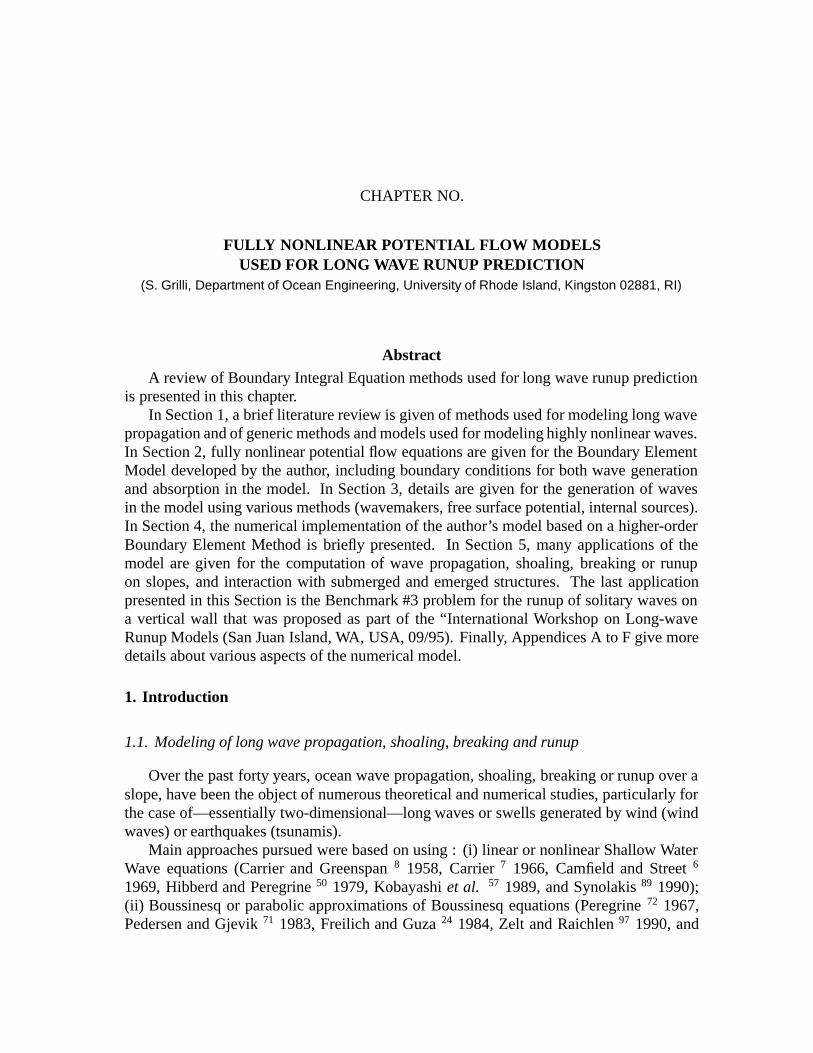
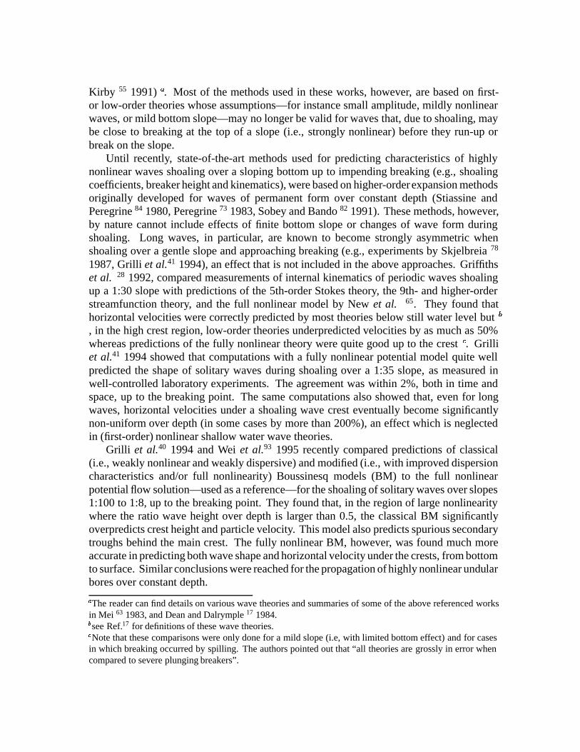
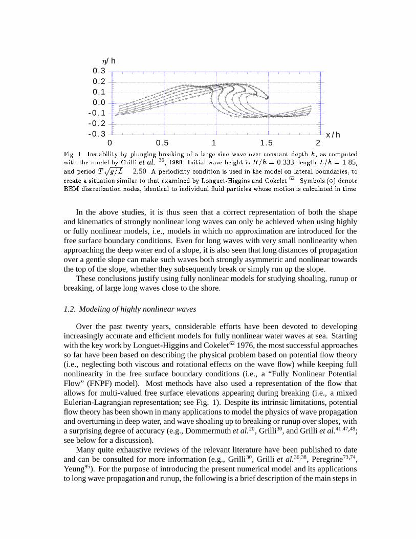
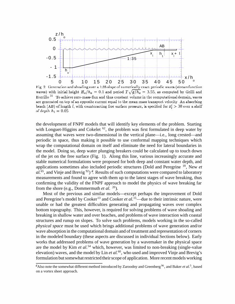
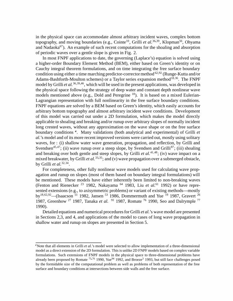
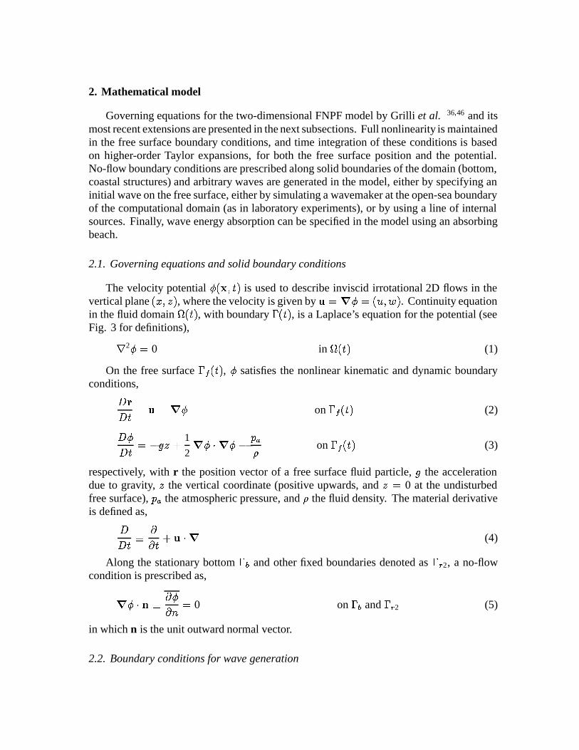
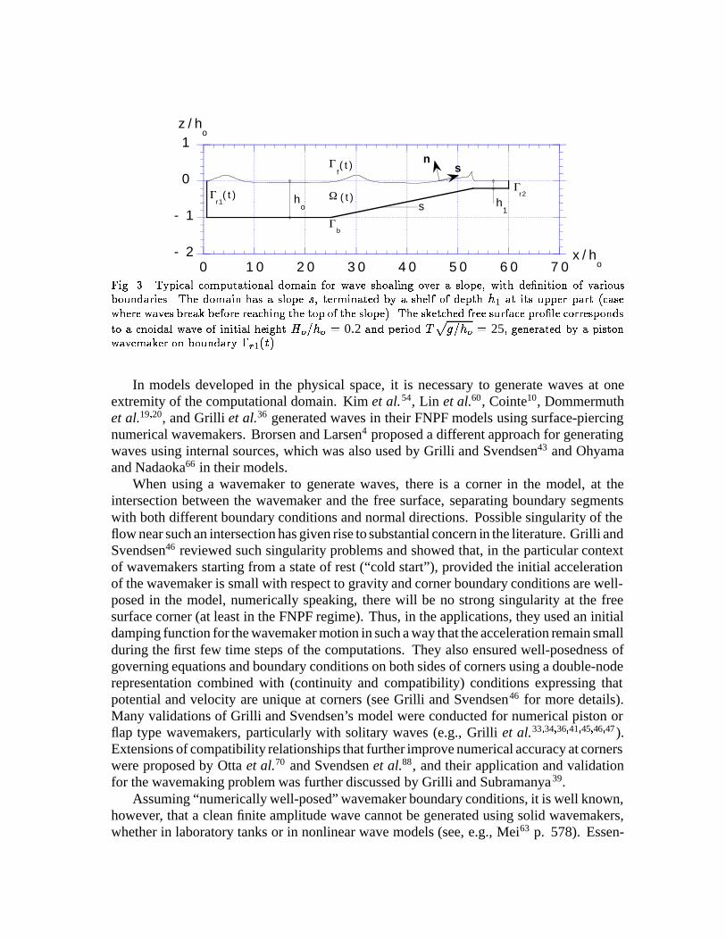
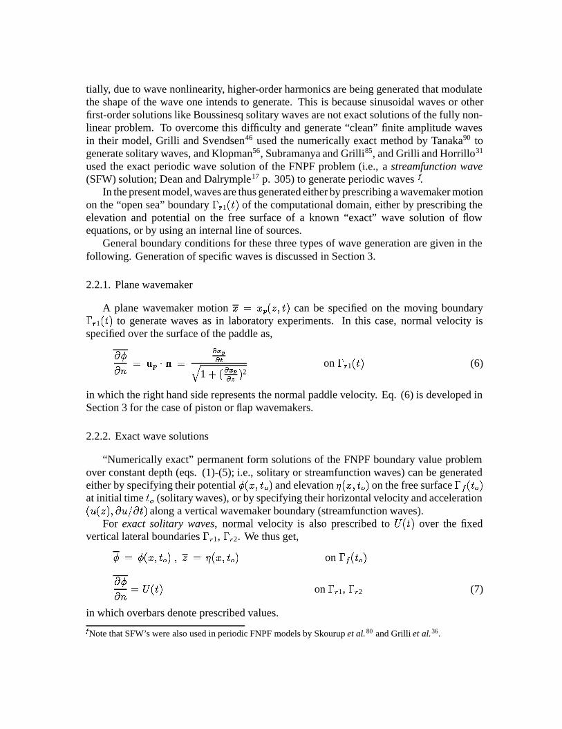
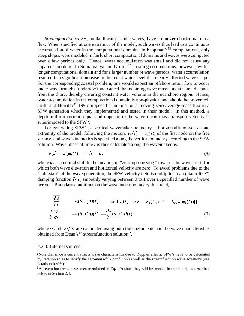
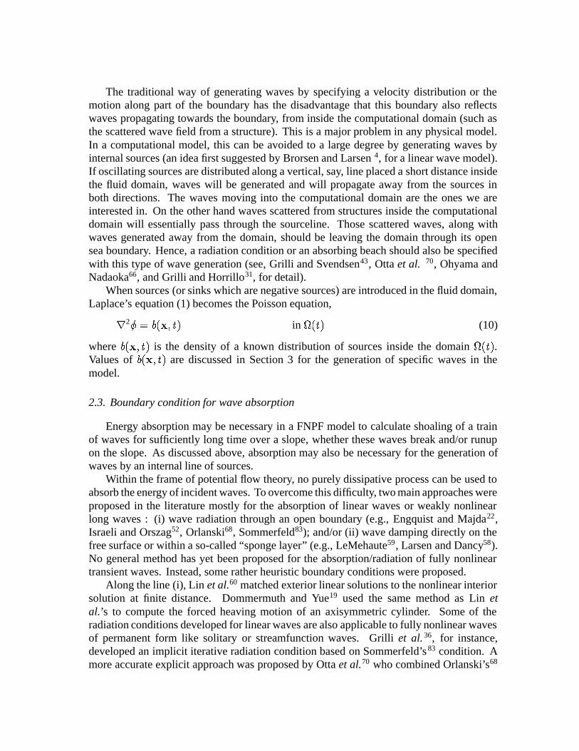
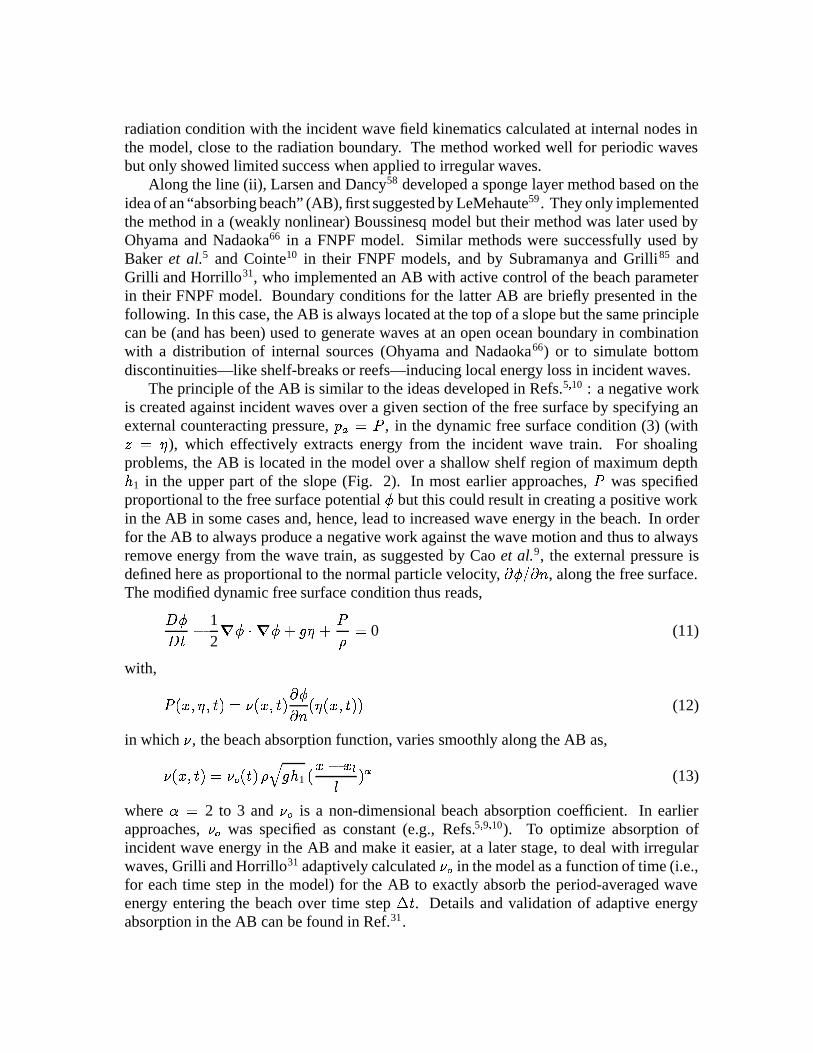
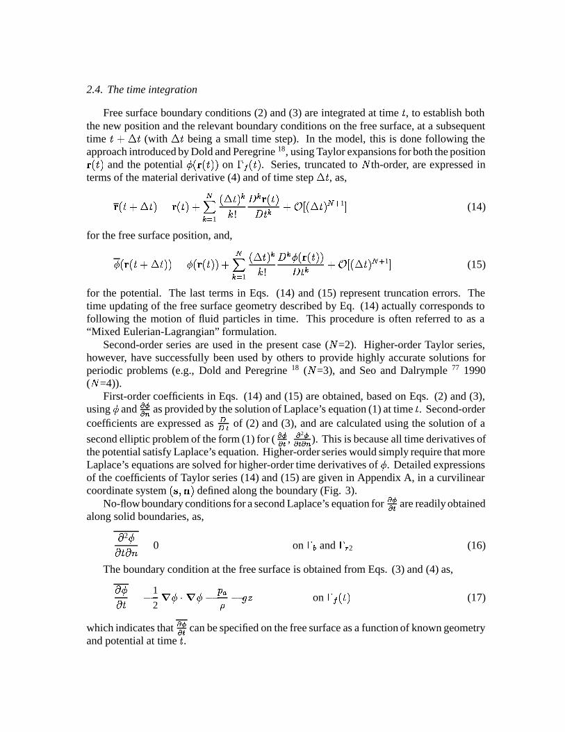
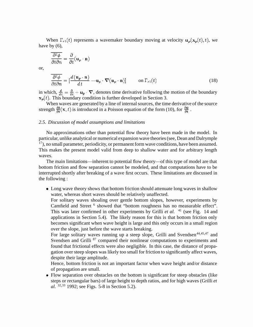
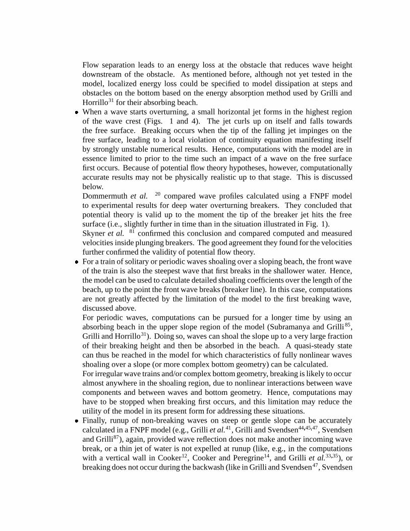
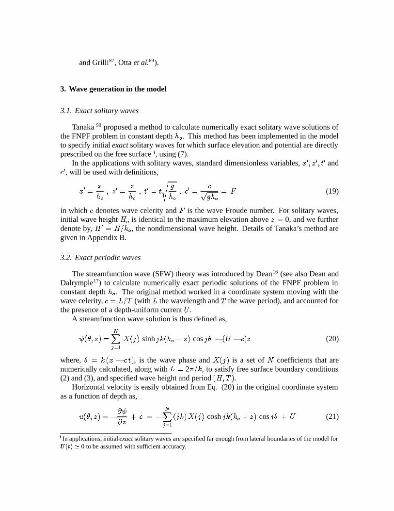
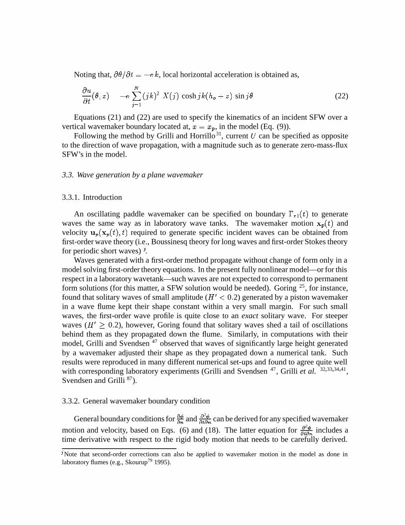
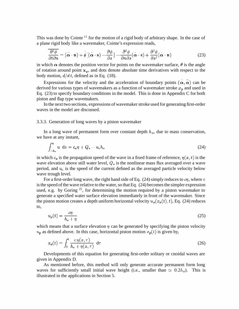
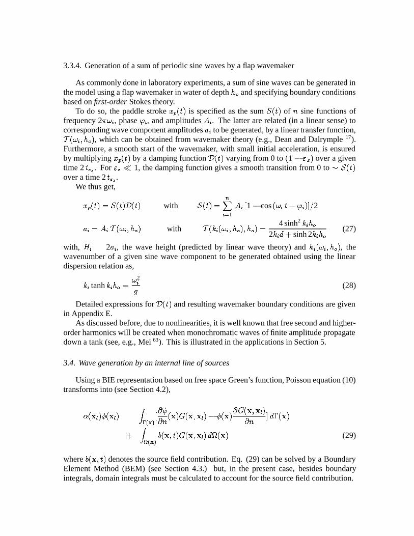
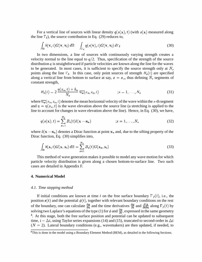
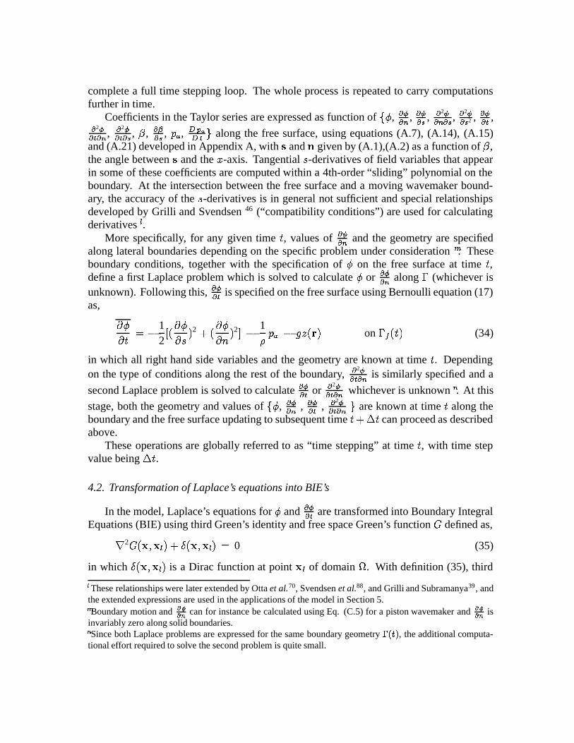
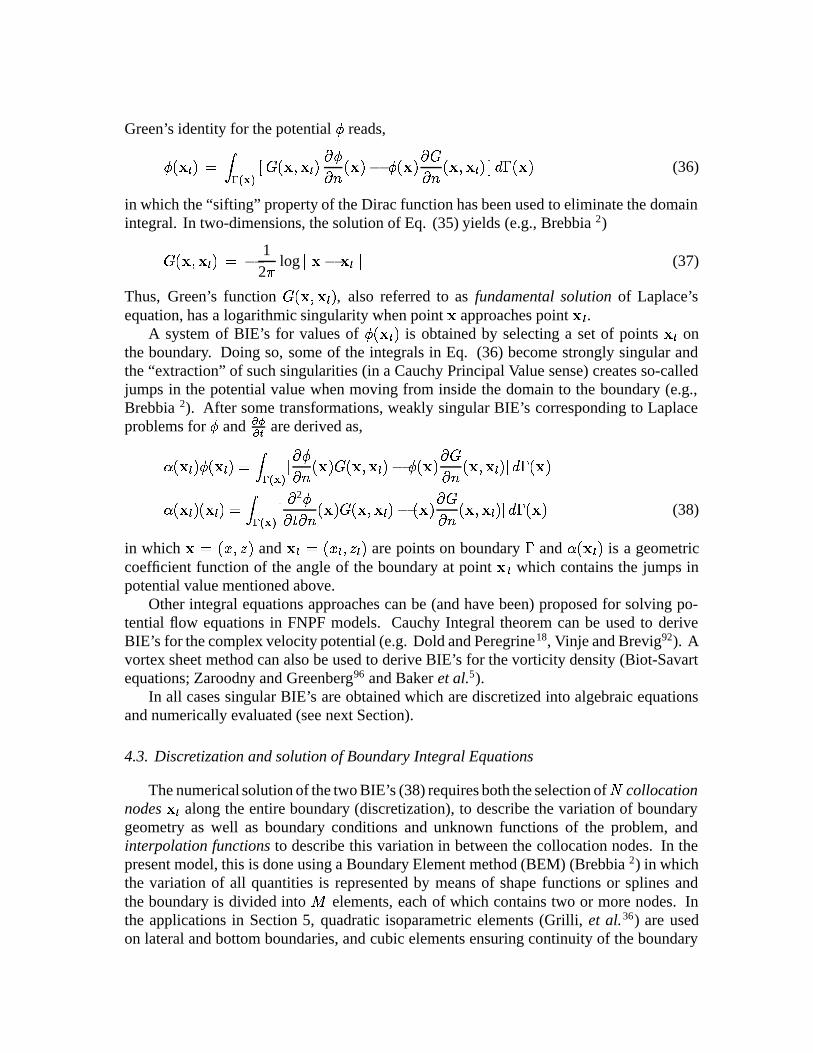
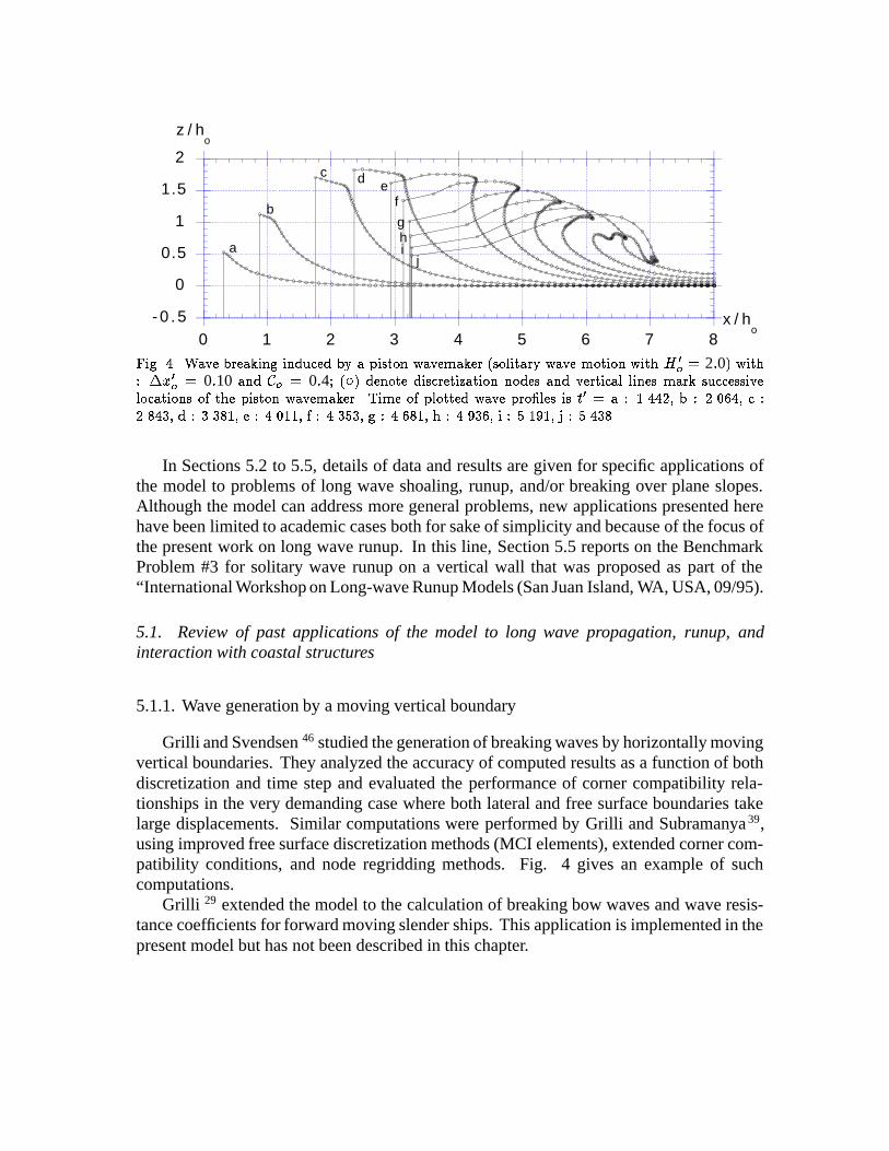
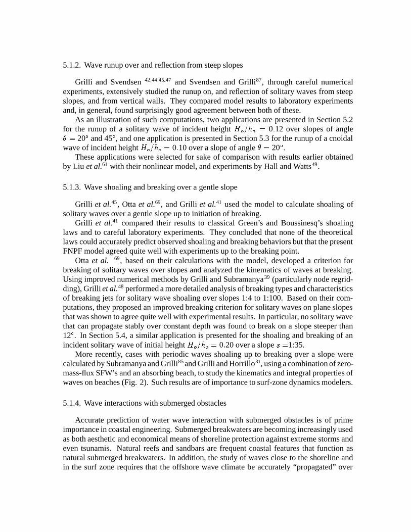
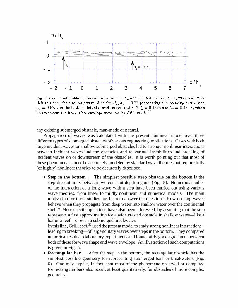
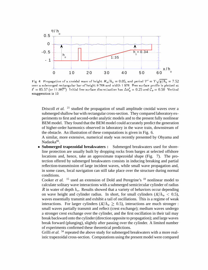
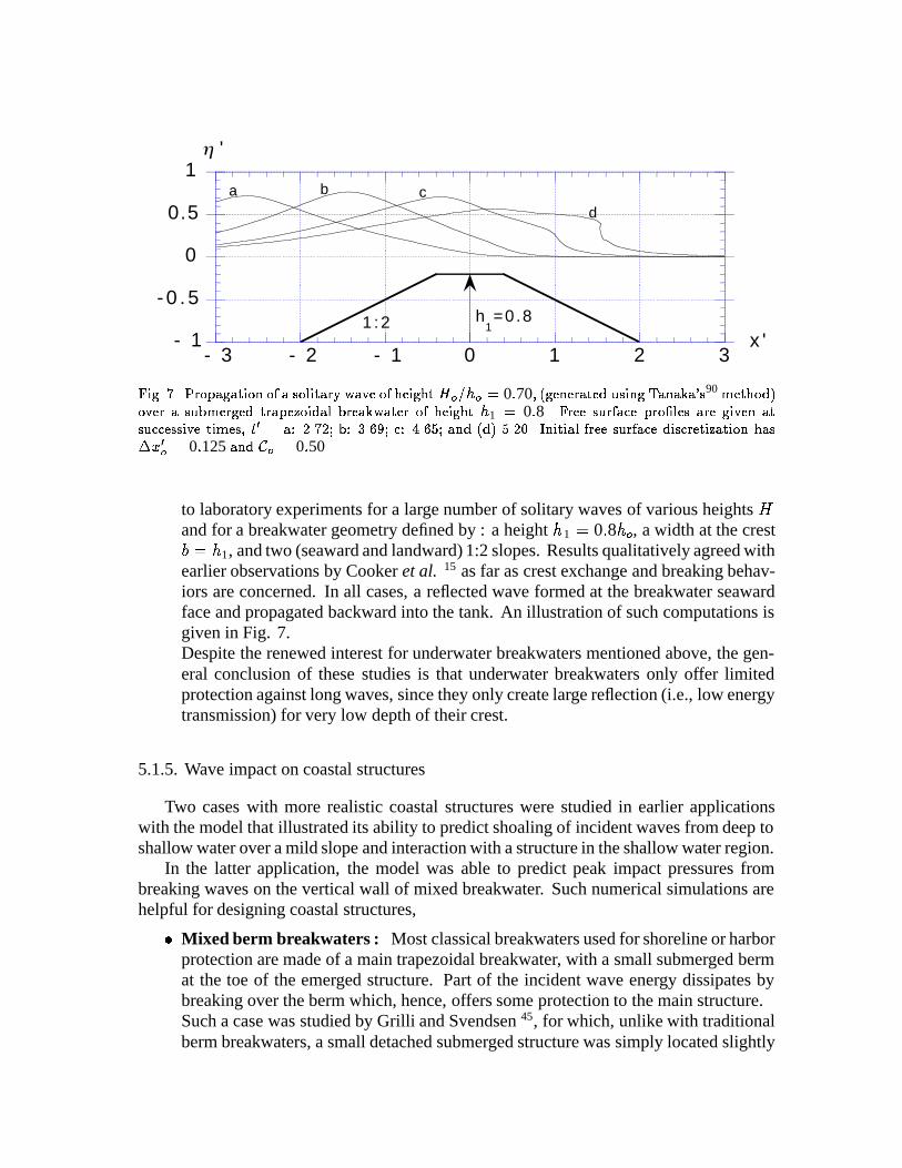
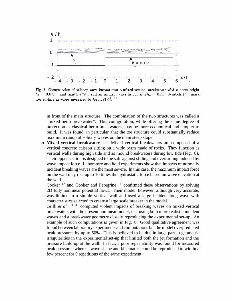
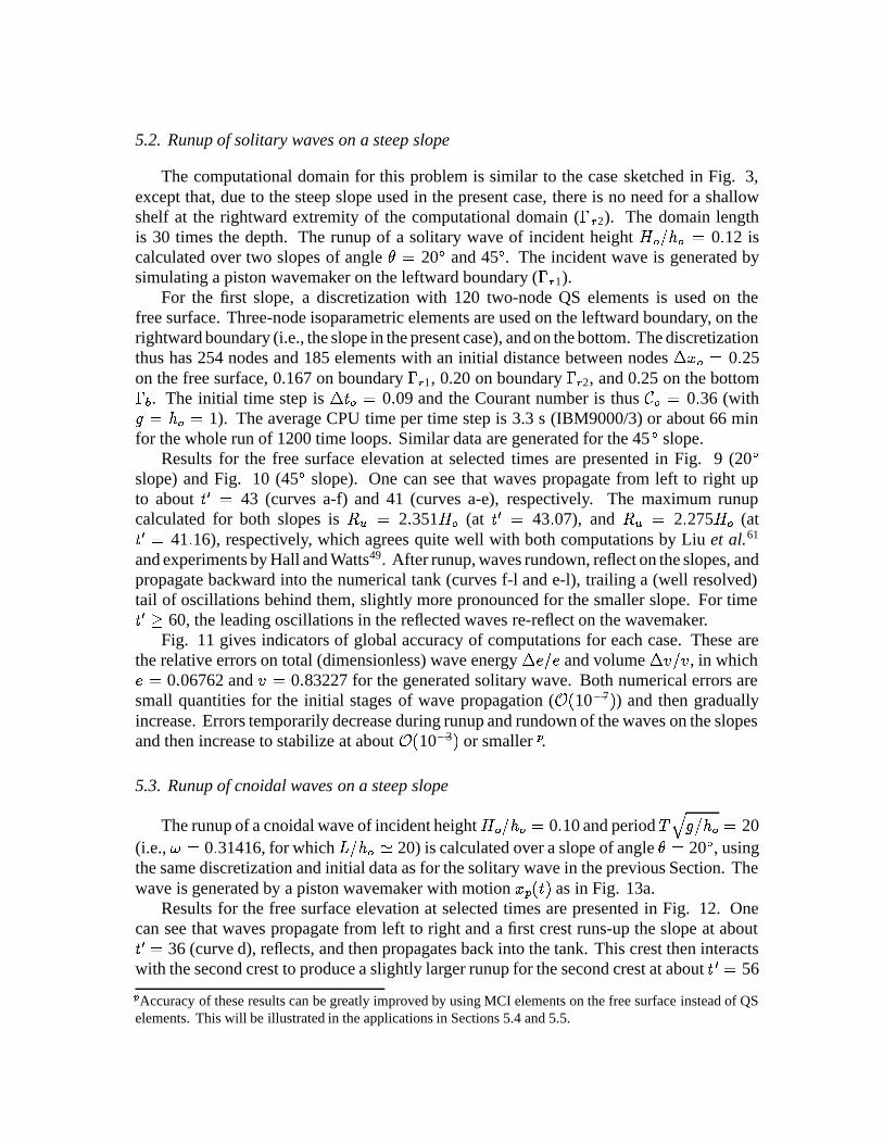
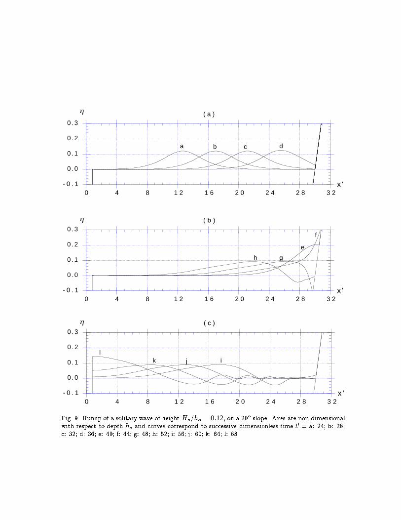
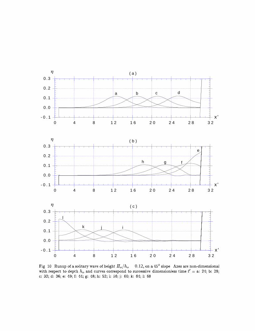
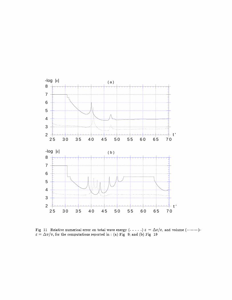
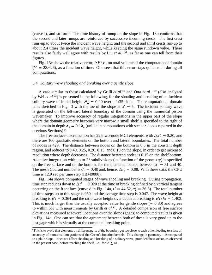
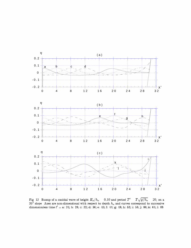
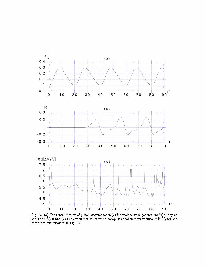
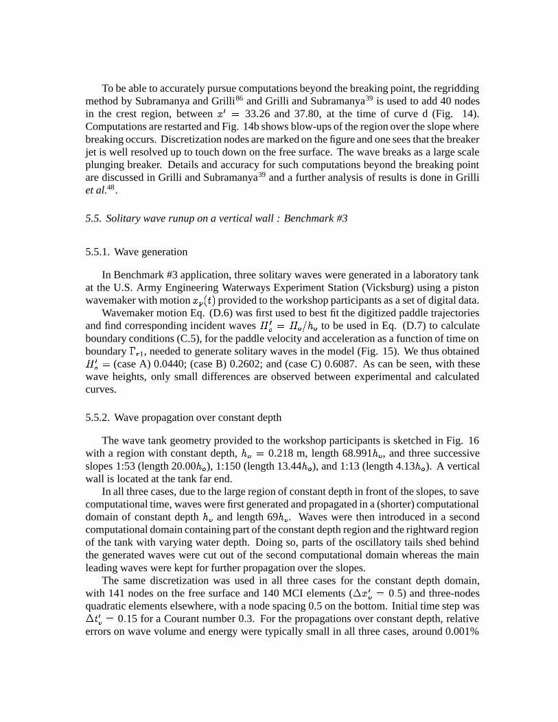
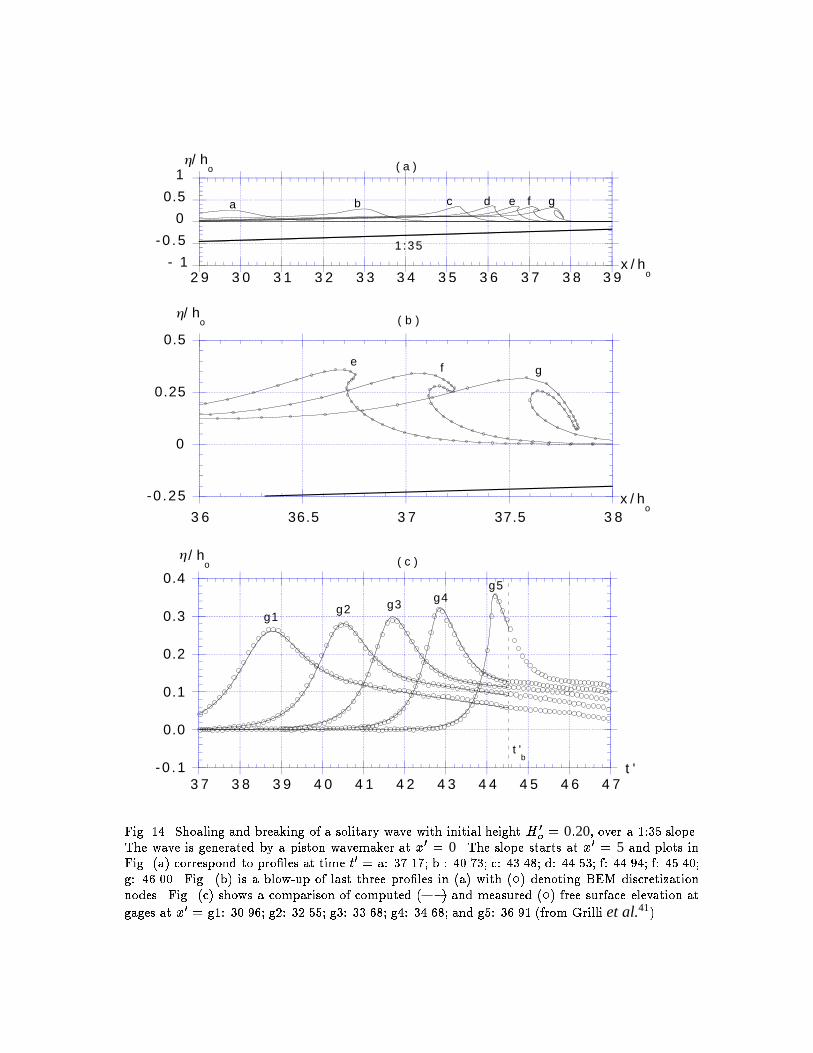
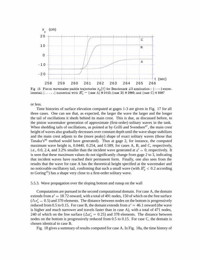
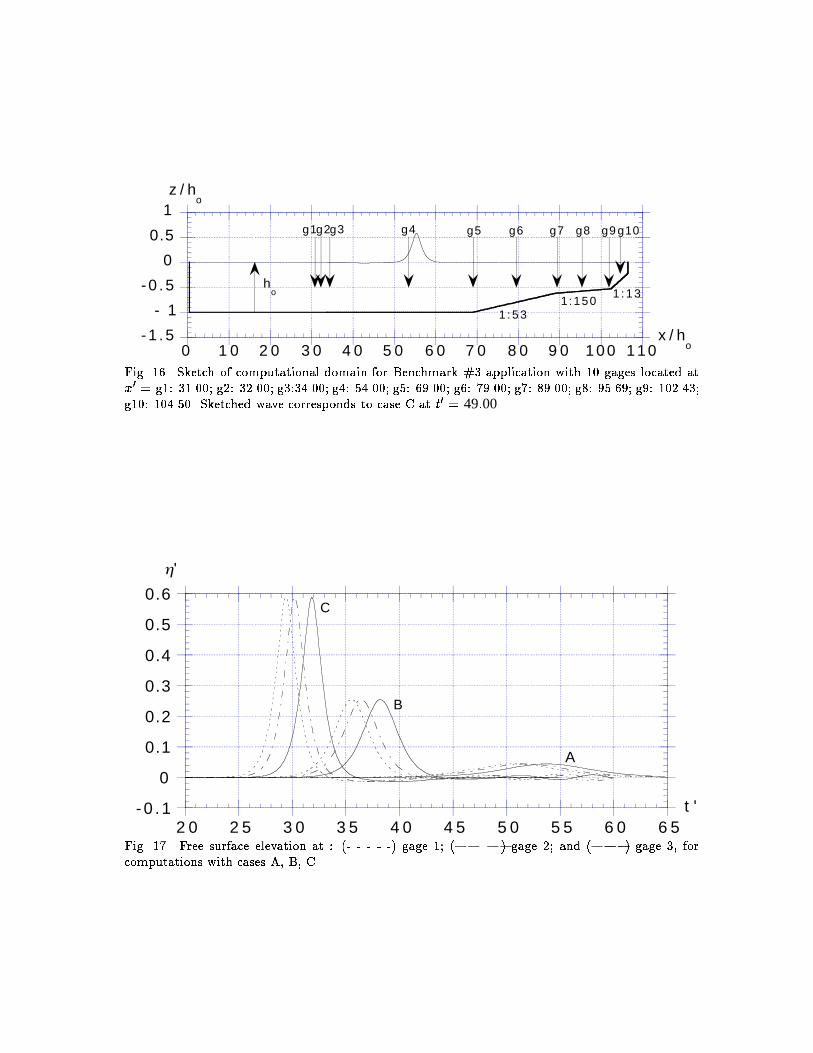
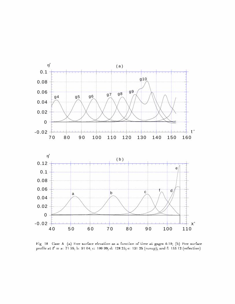
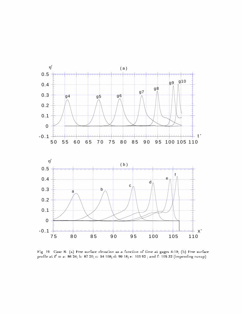
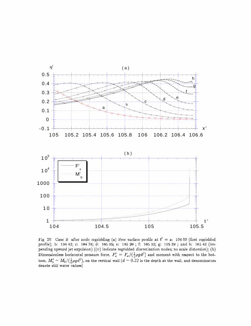
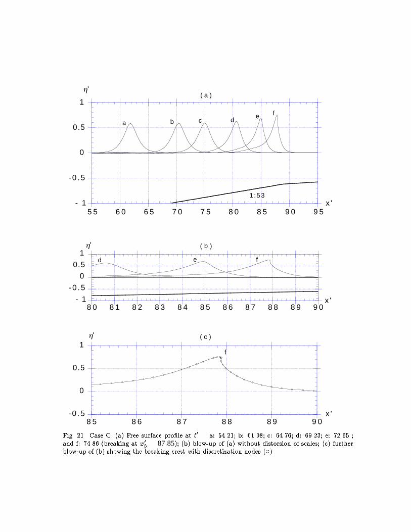
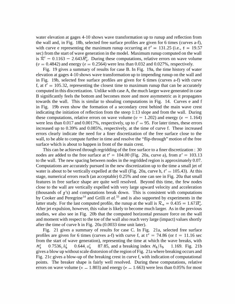
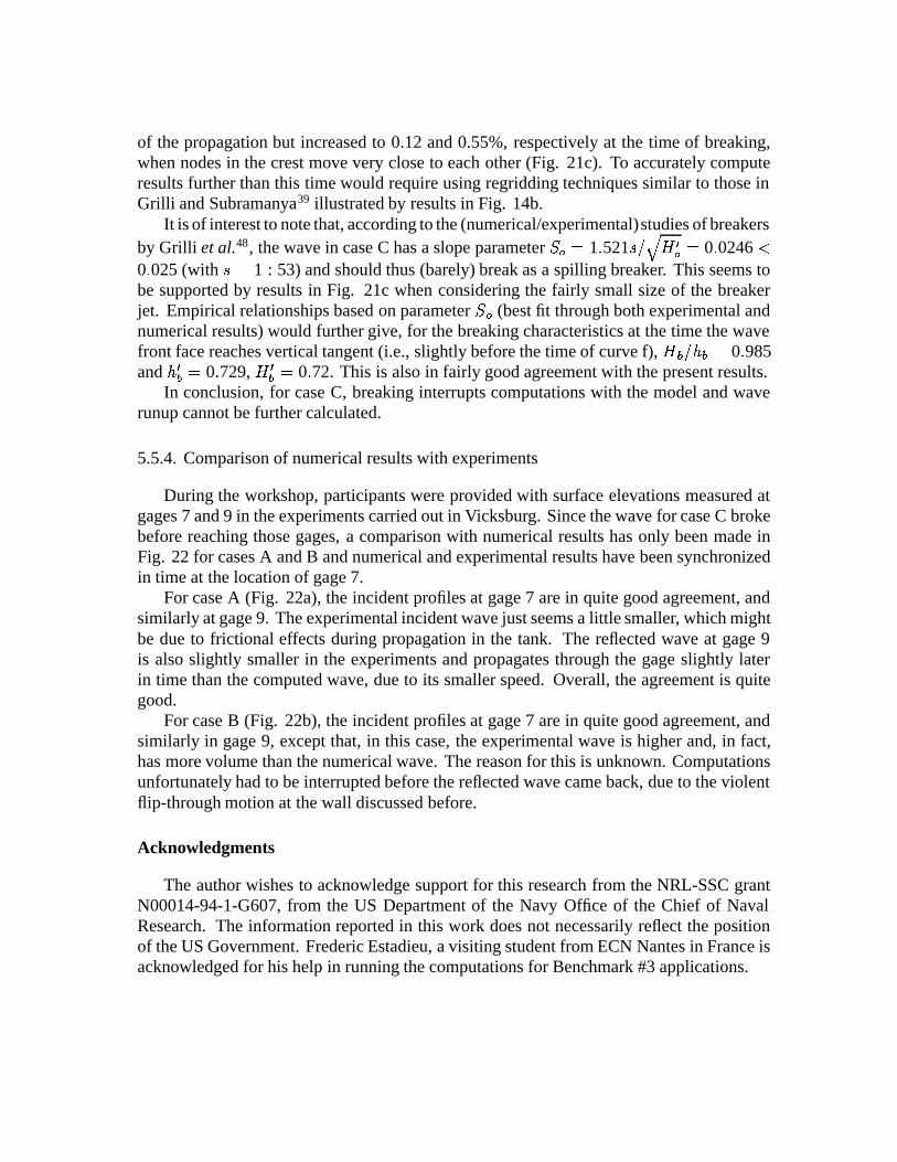
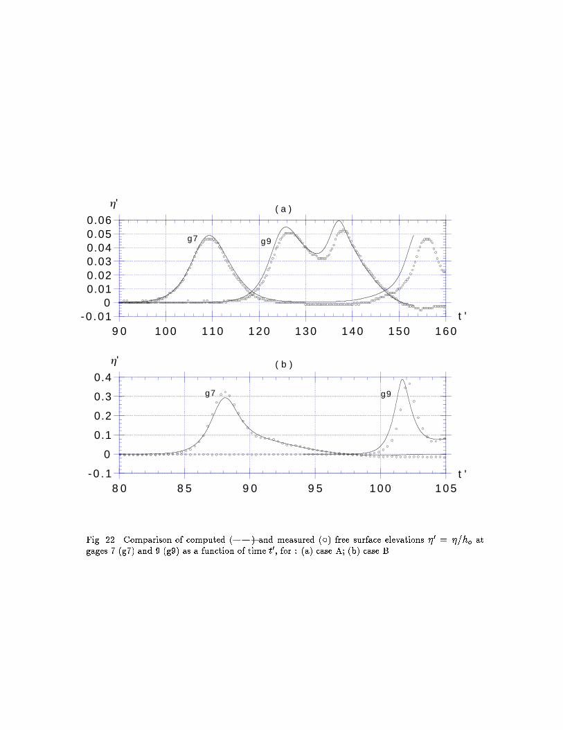
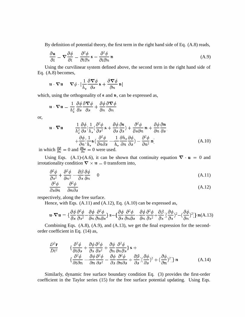
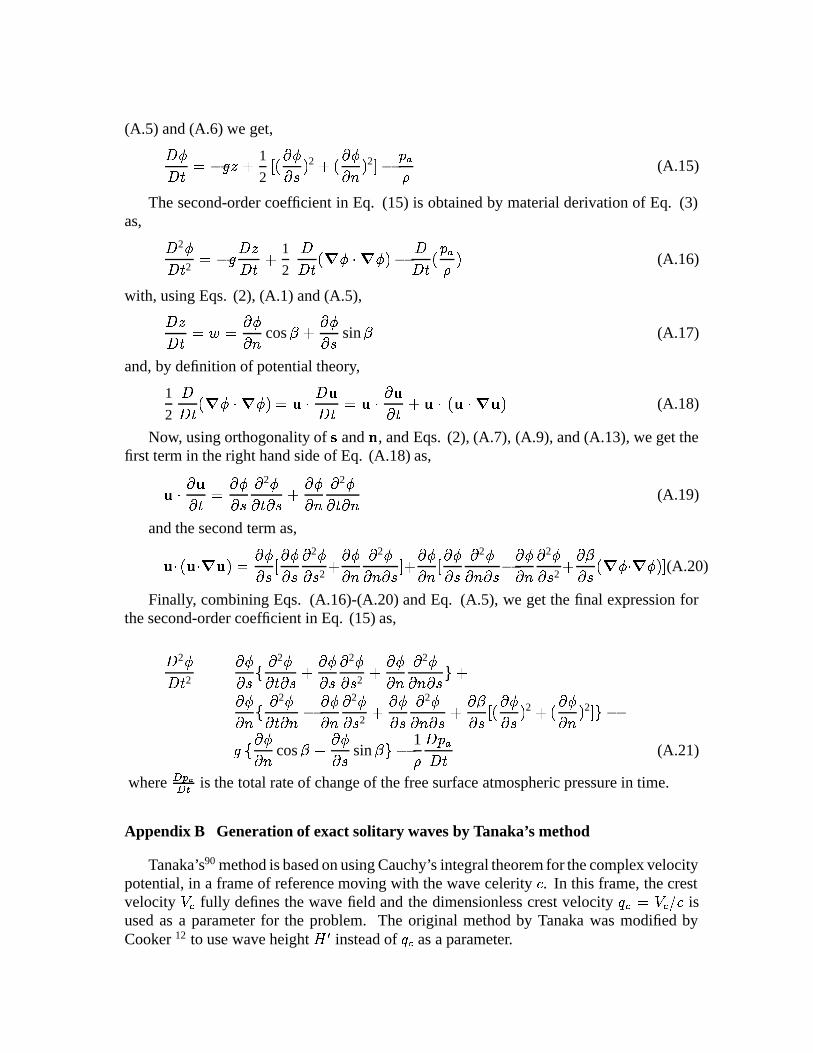
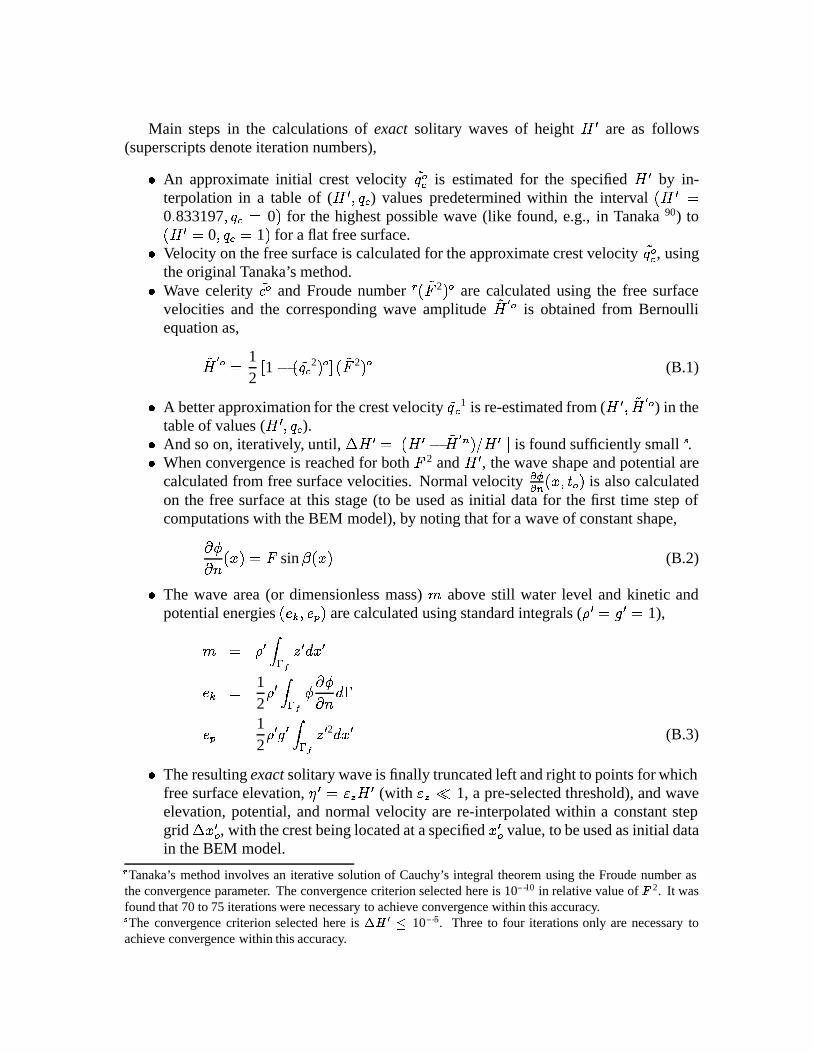
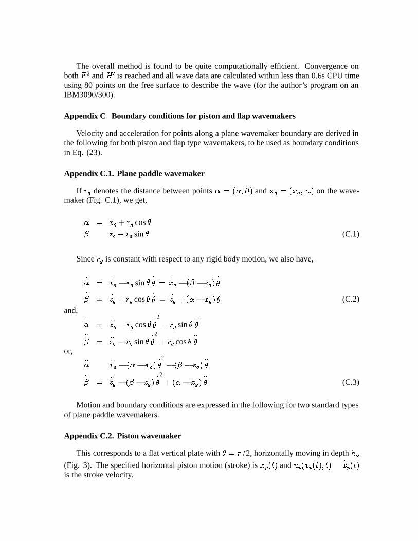
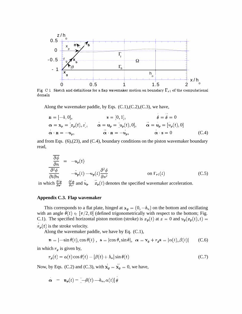
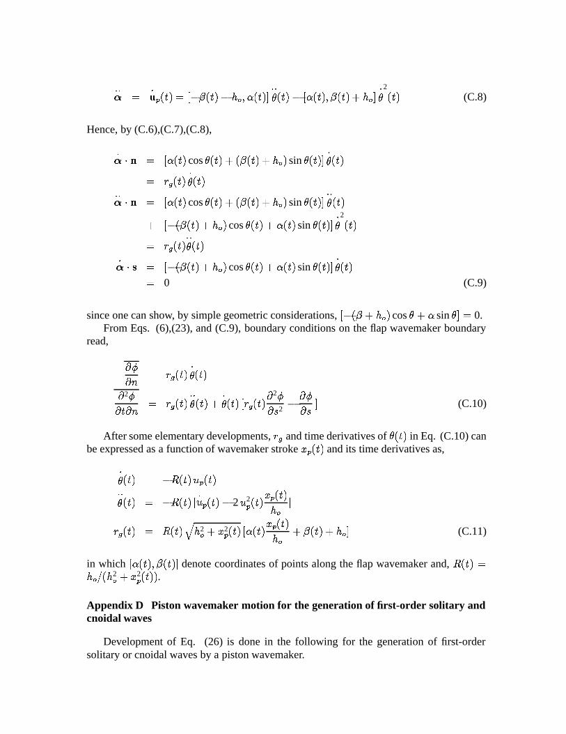
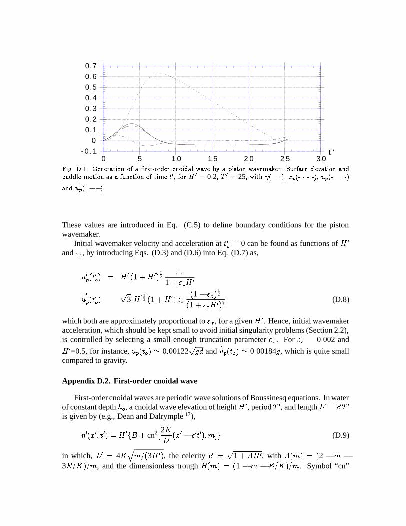
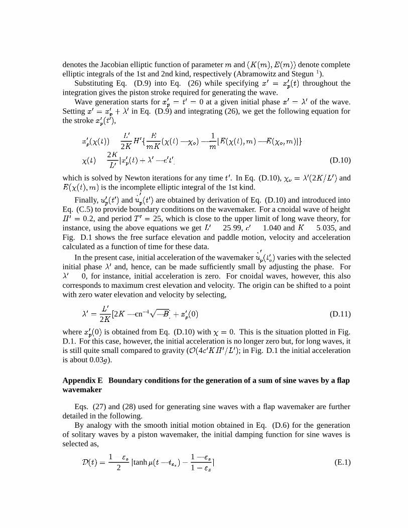
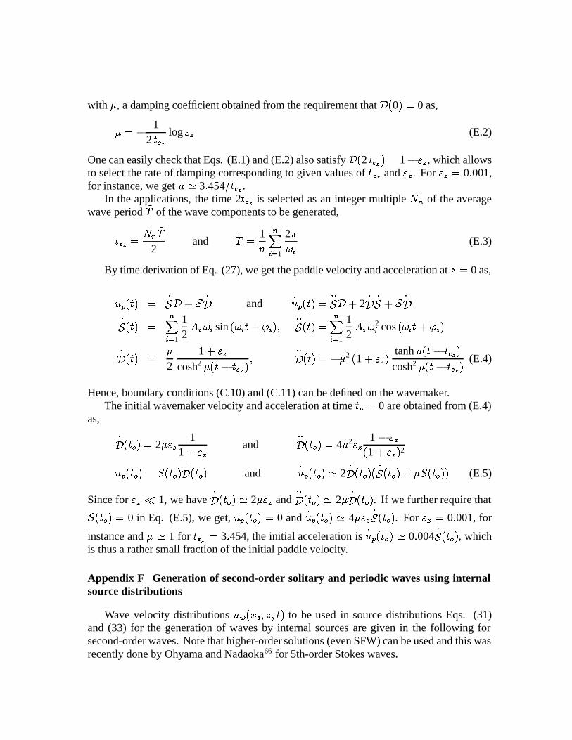
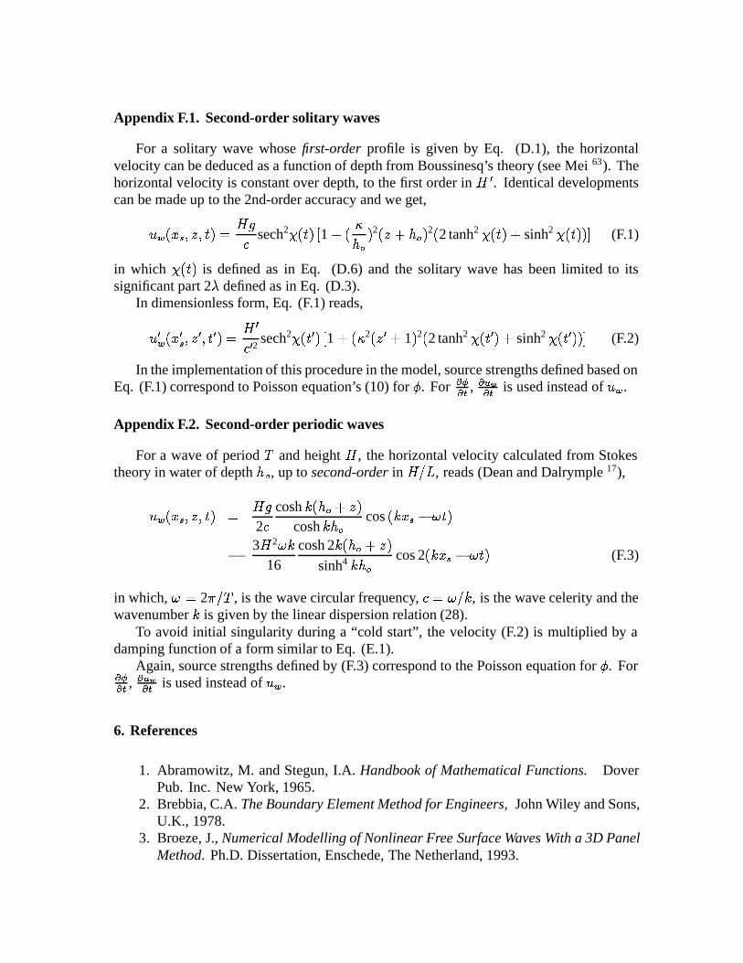
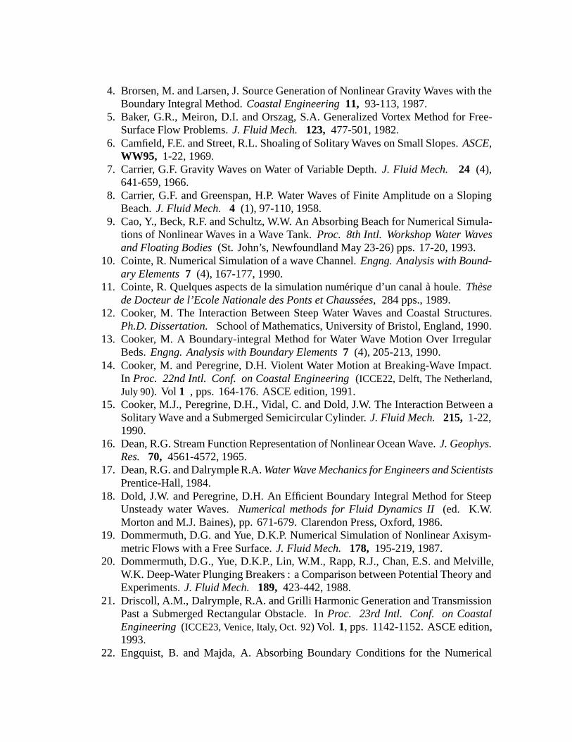
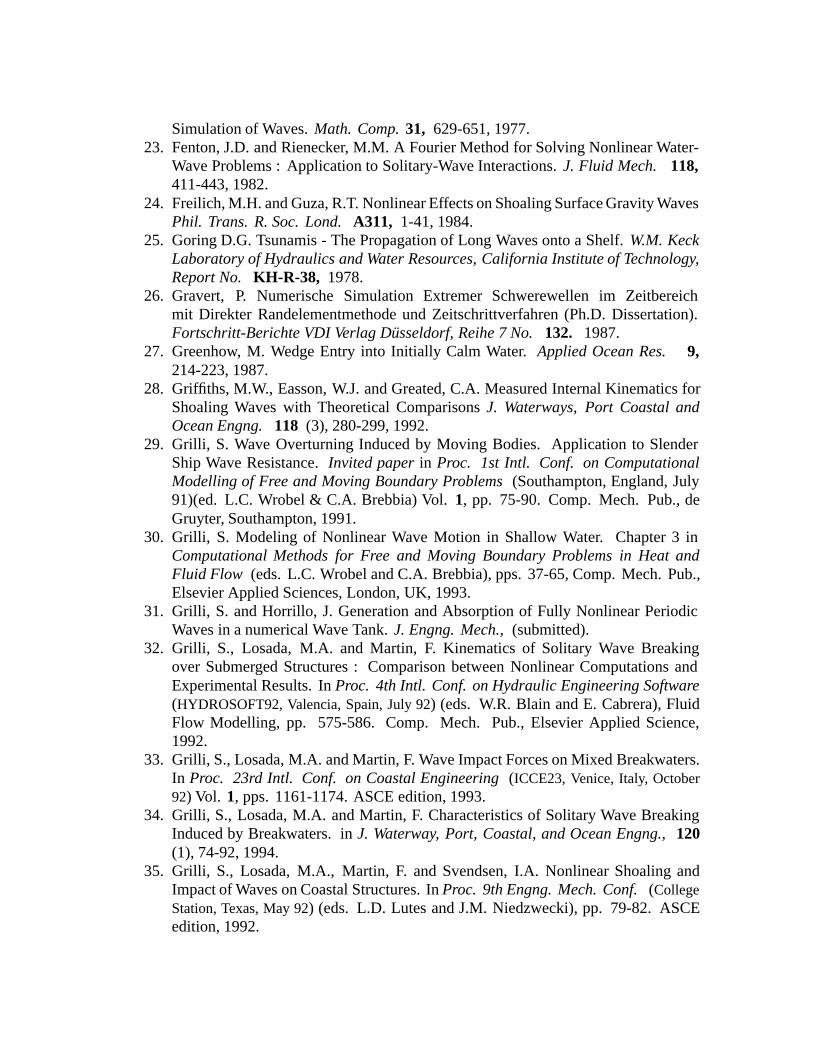
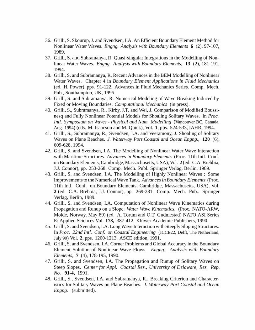
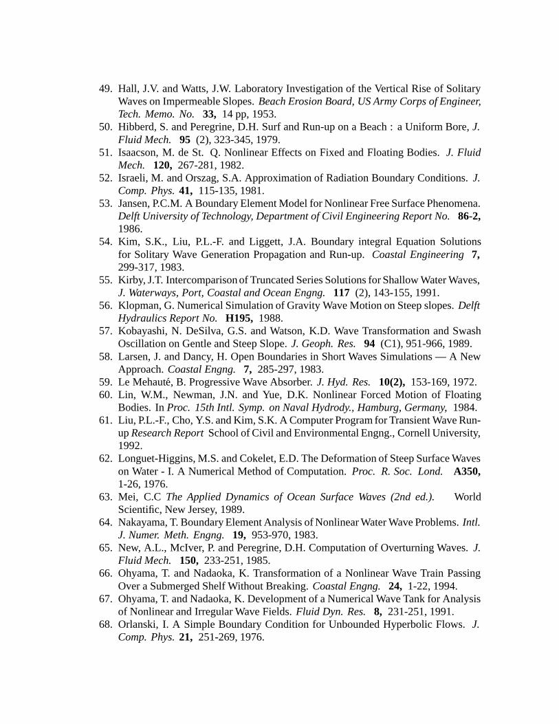
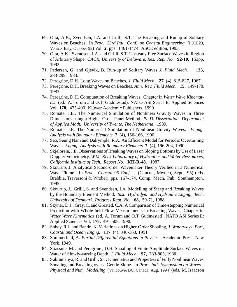
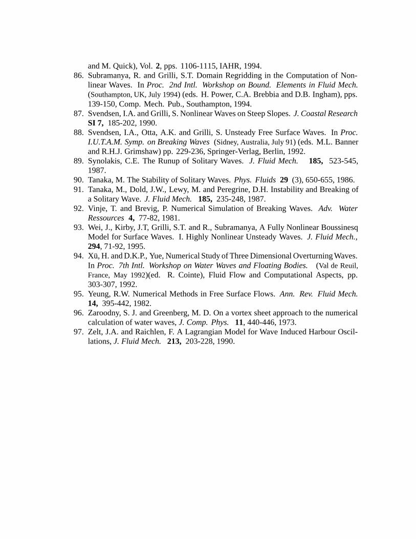


![Existence and regularity results for fully nonlinear ...capde.cmm.uchile.cl/files/2015/07/felmer2012.pdf · for fully nonlinear equations were considered in [14,28]). We could also](https://static.documents.pub/doc/80x56/606d7d5021c6ff4214113677/existence-and-regularity-results-for-fully-nonlinear-capdecmm-for-fully-nonlinear.jpg)


