Page 1
GASEOUS SECONDARY ELECTRON
DETECTION AND CASCADE
AMPLIFICATION IN THE ENVIRONMENTAL
SCANNING ELECTRON MICROSCOPE
By
Scott Warwick Morgan
A THESIS SUBMITTED IN FULFILMENT OF THE
REQUIREMENTS FOR THE DEGREE OF
DOCTOR OF PHILOSOPHY
FACULTY OF SCIENCE
UNIVERSITY OF TECHNOLOGY, SYDNEY
AUSTRALIA
2005
Page 2
Certificate
I certify that the work in this thesis has not previously been submitted for a degree nor
has it been submitted as part of requirements for a degree except as fully acknowledged
within the text.
I also certify that the thesis has been written by me. Any help that I have received
in my research work and the preparation of the thesis itself has been acknowledged.
In addition, I certify that all information sources and literature used are indicated in
the thesis.
Signature of Author
i
Page 4
Acknowledgments
This work in this thesis was conducted under the supervision of Assoc. Prof. Matthew
Phillips, director of the Microstructural Analysis Unit (MAU), University of Tech-
nology, Sydney (UTS). I would like to sincerely thank Assoc. Prof. Phillips for his
undivided help and support during the entirety of my research. His cool, calm and
collected, but rigourous, approach to science made my time spent with him very
learned and enjoyable.
I would like to thank Dr Milos Toth, currently at the FEI company, Boston, for his
ongoing help, fruitful discussions and experimental collaboration both at UTS and
the Polymer and Colloids Group, Cavendish Laboratory, University of Cambridge.
I would also like to thank the staff of the physics department at UTS for valuable
discussions and for the loan of some of the equipment used in experiments. I wish to
thank the staff at the MAU, consisting of Richard Wuhrer, Mark Berkahn and Katie
McBean, for outstanding technical support and friendly advice.
I would especially like to thank my fiance Larissa Lembke for her devoted love
and support over the entire course of my PhD. I am grateful to Larissa for putting
up with my ‘occasional’ bad moods, late nights, missing dinners and proof-reading
this thesis. “Thanks darling”.
I sincerely thank my parents (Warwick and Lynette), nanna (Pearl) for their
utmost moral and financial support, and for continuously being there for me. I also
gratefully thank the other close members of my family and friends for their help,
iii
Page 5
support, physics discussions and for sharing a beer with me when I needed it most.
I apologize to anyone for whom felt at times my PhD was of more importance than
them.
Lastly, I wish to thank Chris Cornell, James Hetfield and my Ibanez RG 450 for
the jam sessions when my brain could not take anymore.
iv
Page 6
Table of Contents
List of Figures viii
List of Tables xix
Nomenclature xxi
Abstract xxxv
1 Introduction 1
2 Background to Environmental Scanning Electron Microscopy 5
2.1 Introduction . . . . . . . . . . . . . . . . . . . . . . . . . . . . . . . . 6
2.2 Vacuum System . . . . . . . . . . . . . . . . . . . . . . . . . . . . . . 8
2.3 Primary Electron Beam-Gas Scattering . . . . . . . . . . . . . . . . . 11
2.3.1 Scattering Cross Sections . . . . . . . . . . . . . . . . . . . . . 12
2.3.2 Primary Electron Beam Transmission . . . . . . . . . . . . . . 23
2.3.3 Electron Distribution and Skirt Profiles . . . . . . . . . . . . . 26
2.4 Signal Detection . . . . . . . . . . . . . . . . . . . . . . . . . . . . . . 36
2.4.1 Induced Signals . . . . . . . . . . . . . . . . . . . . . . . . . . 41
2.4.2 Gaseous Secondary Electron Detector Electronics . . . . . . . 50
3 Gaseous Cascade Amplification in Partially Ionized Gases - Townsend
Gas Capacitor Model 54
3.1 Introduction . . . . . . . . . . . . . . . . . . . . . . . . . . . . . . . . 55
3.2 General Overview of Cascade Amplification . . . . . . . . . . . . . . 56
3.3 Cascade Amplification of Electrons . . . . . . . . . . . . . . . . . . . 59
3.4 Cascade Amplification of Primary Electrons . . . . . . . . . . . . . . 61
3.5 Cascade Amplification of Backscattered Electrons . . . . . . . . . . . 63
3.6 Cascade Amplification of Secondary Electrons . . . . . . . . . . . . . 64
v
Page 7
3.7 Cascade Amplification of Secondary Electrons Generated by Ion, Pho-
ton, Metastable and Neutral Molecule Surface Collisions . . . . . . . 65
3.8 Electron Impact Ionization Cross sections . . . . . . . . . . . . . . . . 75
3.9 Ionization Efficiency of Primary and Backscattered Electrons . . . . . 80
3.10 Ionization Efficiency of Secondary and Environmental Electrons - First
Townsend Ionization Coefficient . . . . . . . . . . . . . . . . . . . . . 81
3.11 Gaseous Cascade Amplification Profiles . . . . . . . . . . . . . . . . . 85
4 Transient Analysis of Gaseous Electron-Ion Recombination in the
Environmental Scanning Electron Microscope 98
4.1 Introduction . . . . . . . . . . . . . . . . . . . . . . . . . . . . . . . . 99
4.2 Theory . . . . . . . . . . . . . . . . . . . . . . . . . . . . . . . . . . . 101
4.2.1 Gaseous Electron-Ion Recombination . . . . . . . . . . . . . . 101
4.3 Transient SE-Ion Recombination Model . . . . . . . . . . . . . . . . . 109
4.4 Experimental Techniques . . . . . . . . . . . . . . . . . . . . . . . . . 117
4.4.1 Measurement of Electronic Gas Amplification . . . . . . . . . 118
4.4.2 Determination of Recombination Coefficients, Recombination
Rates, Ionization Rates, Electron Drift Velocities and Time
Constants . . . . . . . . . . . . . . . . . . . . . . . . . . . . . 120
4.5 Preamble . . . . . . . . . . . . . . . . . . . . . . . . . . . . . . . . . 122
4.6 Results and Discussion . . . . . . . . . . . . . . . . . . . . . . . . . . 132
4.6.1 Generation Rates . . . . . . . . . . . . . . . . . . . . . . . . . 132
4.6.2 Electron Drift Velocities . . . . . . . . . . . . . . . . . . . . . 136
4.6.3 Recombination Coefficients . . . . . . . . . . . . . . . . . . . . 138
4.6.4 Recombination Rates . . . . . . . . . . . . . . . . . . . . . . . 142
4.6.5 Time Constants . . . . . . . . . . . . . . . . . . . . . . . . . . 144
4.7 Future Work . . . . . . . . . . . . . . . . . . . . . . . . . . . . . . . . 146
4.8 Conclusions . . . . . . . . . . . . . . . . . . . . . . . . . . . . . . . . 148
5 A Preliminary Investigation of Gaseous Scintillation Detection and
Amplification in Environmental SEM 150
5.1 Introduction . . . . . . . . . . . . . . . . . . . . . . . . . . . . . . . . 151
5.2 Theory . . . . . . . . . . . . . . . . . . . . . . . . . . . . . . . . . . . 153
5.2.1 Gaseous Proportional Scintillation and Electroluminescence . . 153
5.3 Gaseous Scintillation and Electroluminescence Amplification Model . 159
5.4 Experimental Techniques . . . . . . . . . . . . . . . . . . . . . . . . . 164
5.4.1 Determination of Photon Amplification . . . . . . . . . . . . . 166
5.4.2 Determination of Electronic Amplification . . . . . . . . . . . 171
5.5 Results and Discussion . . . . . . . . . . . . . . . . . . . . . . . . . . 173
vi
Page 8
5.5.1 Images Obtained Using GSD and GSED . . . . . . . . . . . . 173
5.5.2 Photon and Electronic Amplification Using the GSED to Gen-
erate Gaseous Scintillation . . . . . . . . . . . . . . . . . . . . 179
5.5.3 Photon and Electronic Amplification Using the GSD to Gener-
ate Gaseous Scintillation - Enhancement of Photon Collection
Utilizing Electrostatic Focusing . . . . . . . . . . . . . . . . . 190
5.6 Future Work . . . . . . . . . . . . . . . . . . . . . . . . . . . . . . . . 197
5.7 Conclusions . . . . . . . . . . . . . . . . . . . . . . . . . . . . . . . . 198
6 Photon Emission Spectra of Electroluminescent Imaging Gases Com-
monly Utilized in the Environmental SEM 200
6.1 Introduction . . . . . . . . . . . . . . . . . . . . . . . . . . . . . . . . 201
6.2 Experimental Techniques . . . . . . . . . . . . . . . . . . . . . . . . . 203
6.3 Results and Analysis . . . . . . . . . . . . . . . . . . . . . . . . . . . 205
6.3.1 Emission Spectra of Argon . . . . . . . . . . . . . . . . . . . . 205
6.3.2 Emission Spectra of Nitrogen . . . . . . . . . . . . . . . . . . 208
6.4 Conclusions . . . . . . . . . . . . . . . . . . . . . . . . . . . . . . . . 211
A Atomic and Molecular Collisions in Partially Ionized Gases 213
Bibliography 225
vii
Page 9
List of Figures
2.1 Schematic diagram showing the ESEM vacuum system. The vacuum
system consists of five stages of increasing vacuum level. The stages
are the specimen chamber, first environmental chamber (EC1), second
environmental chamber (EC2), electron column and electron gun. The
column and chamber regions are separated by two pressure limiting
apertures (PLAs). The PLAs are placed close together to minimize
PE scattering (adapted from Philips Electron Optics (1996)). [IP=ion
pump, DP=diffusion pump, RT=rotary pump] . . . . . . . . . . . . . 10
2.2 Differential scattering cross section dσ/dΩ (elastic, inelastic and total)
versus scattering angle θ in argon (Ar) (adapted from Danilatos (1988)
and Jost & Kessler (1963)). [εPE = 30 keV] . . . . . . . . . . . . . . 17
2.3 Total scattering cross section (σsT ) of monotonic (argon (Ar)), diatomic
(nitrogen (N2)) and polyatomic (water vapour (H2O)) gases versus
primary electron beam energy (εPE) (Danilatos 1988, Jost & Kessler
1963). . . . . . . . . . . . . . . . . . . . . . . . . . . . . . . . . . . . 20
2.4 Experimentally obtained total scattering cross sections (σsT ) versus pri-
mary electron beam energy (εPE) for water vapour (H2O) and nitrogen
(N2) (Phillips et al. 1999). [d = 6.5 mm, T = 298 K] . . . . . . . . . 23
viii
Page 10
2.5 Schematic diagram illustrating the scattering regimes for an electron
beam traversing a gaseous medium. A conventional high vacuum SEM
operates in the ‘minimal scattering regime’ whilst an ESEM operates
in the ‘partial scattering regime’. Complete scattering of the PE beam
conveys no useful image information (taken from Philips Electron Op-
tics 1996). . . . . . . . . . . . . . . . . . . . . . . . . . . . . . . . . . 24
2.6 Experimental primary electron beam transmission (unscattered probe
current (I0PE) to beam current (IPE) ratio) versus (a) nitrogen pressure
(pN2) and (b) water vapour pressure (pH2O) at various primary electron
beam energies (εPE) (Phillips et al. 1999). [d = 6.45 mm, T = 298 K] 27
2.7 Schematic diagram illustrating PE-gas scattering in the ESEM. A PE
of energy εPE undergoing a collision with a gas atom or molecule be-
tween z and z + dz is scattered through an angle θ and θ + dθ into
the solid angle dΩ. The scattered PE then strikes the sample surface
between r and r + dr (Danilatos 1988, Kadoun et al. 2003). . . . . . 28
2.8 Theoretical plural scattering normalized beam intensity versus radial
distance (r) from beam center for an infinitely thin electron beam (delta
function) in argon (Ar) acquired as a function of argon pressure (pAr)
(adapted from Danilatos 1988 and Jost & Kessler 1963). [εPE = 50
keV, d = 6.45 mm, T = 298 K] . . . . . . . . . . . . . . . . . . . . . . 32
2.9 Experimental normalized beam intensity versus radial distance (r)
from beam center acquired as a function of (a) nitrogen pressure (pN2)
and (b) water vapour pressure (pH2O) (Phillips et al. 1999). [εPE = 30
keV, d = 10.0 mm] . . . . . . . . . . . . . . . . . . . . . . . . . . . . 33
ix
Page 11
2.10 Theoretical plural scattering skirt half radius (r1/2) versus argon pres-
sure (pAr) and sample-electrode separation (d) for an infinitely thin
electron beam in argon (Ar) (adapted from Danilatos 1988 and Jost &
Kessler 1963). [εPE = 50 keV, T = 298 K] . . . . . . . . . . . . . . . 35
2.11 Image showing the gaseous secondary electron detector (GSED). The
suppressor electrode is placed at +9 volts relative to the ring voltage
to discriminate against backscattered and type III secondary electrons. 37
2.12 Schematic diagram showing the various signals used to generate gaseous
secondary electron detector (GSED) and induced stage current (ISC)
images in an ESEM. Primary beam electrons (PEs) generate secondary
electrons (SEs) and backscattered electrons (BSEs) which ionize gas
molecules producing positive ions (PIs) and environmental secondary
electrons (ESEs). These signals induce current flows IGSED and IISC
in the ring and stage, respectively, which are then amplified to produce
images. . . . . . . . . . . . . . . . . . . . . . . . . . . . . . . . . . . . 39
2.13 Schematic diagram showing the generation of the induced signals IGSED
and IISC by a particle of charge −e traversing the gap in a typi-
cal ESEM containing distributed capacitances and resistances. The
gaseous secondary electron detector (GSED) and induced stage cur-
rent (ISC) amplifiers have time constants R1C1 and R2C2, respectively.
The time constant of an insulating sample is R3C3. The GSED or ISC
electronics can be represented by an equivalent circuit of total time
constant RC. [d = sample-electrode separation, ds = particle dis-
placement, E = electric field, vd = drift velocity, R = resistance, C =
capacitance] . . . . . . . . . . . . . . . . . . . . . . . . . . . . . . . . 40
x
Page 12
2.14 Voltage signal (VS) versus time (t) at various time constants (RC)
when an electron and a positive ion (PI) of transit times Γe and Γi, re-
spectively, are accelerated across a potential difference (V ) after being
released in the center of the gap. For clarity, the drift velocity of the
electron was set to twice that of the ion (ve = 2vi or Γe = Γi/2). . . . 47
2.15 Schematic diagram of the gaseous secondary electron detector (GSED)
preamplifier circuit (adapted from Philips Electron Optics 1997). . . . 51
3.1 Second Townsend coefficient (γ) versus reduced electric field (E/p) for
various gases (nitrogen (N2), argon (Ar)) and cathode materials (Pt,
Na, Cu, Fe) (adapted from von Engel 1965) . . . . . . . . . . . . . . 71
3.2 Total electron impact ionization cross sections (σiT ) for argon (Ar) as
a function of electron energy (ε). Experimentally and theoretically
obtained cross sections are represented by points and line plots, re-
spectively (Asundi & Kurepa 1963, Fletcher & Cowling 1972, Mark
1982, Rapp & Englander-Golden 1965, Schram et al. 1966, Smith
1930, Srinivasan & Rees 1967, Straub et al. 1995, Wallace et al. 1973). 76
3.3 Total electron impact ionization cross sections (σiT ) for nitrogen (N2)
as a function of electron energy (ε). Experimentally and theoretically
obtained cross sections are represented by points and line plots, re-
spectively (Deutsch et al. 2000, Hwang et al. 1996, Khare & Meath
1987, Krishnakumar & Srivastava 1992, Rapp & Englander-Golden
1965, Saksena et al. 1997a, Saksena et al. 1997b, Schram et al. 1965,
Schram et al. 1966, Straub et al. 1996). [BEB=binary-encounter-
Bethe method, BED=binary-encounter-dipole method] . . . . . . . . 77
xi
Page 13
3.4 Total electron impact ionization cross sections (σiT ) for water vapour
(H2O) as a function of electron energy (ε). Experimentally and the-
oretically obtained cross sections are represented by points and line
plots, respectively (Bolorizadeh & Rudd 1986, Deutsch et al. 2000,
Djuric et al. 1988, Hwang et al. 1996, Jain & Khare 1976, Kim &
Rudd 1994, Saksena et al. 1997a, Saksena et al. 1997b, Schutten et al.
1966, Straub et al. 1998, Terrissol et al. 1989). . . . . . . . . . . . . . 78
3.5 First Townsend ionization coefficient (αion(z)) versus gap distance (z)
traversed, acquired as a function of (a) water vapour pressure (pH2O)
[VGSED = 290 V] and (b) gaseous secondary electron detector bias
(VGSED) [p = 1 torr]. Region I: minimal ionization; Region II: increas-
ing ionization efficiency; Region III: the attainment of swarm condi-
tions (adapted from Thiel et al. 1997). . . . . . . . . . . . . . . . . . 83
3.6 Total electronic amplification (Ae) versus water vapour pressure (pH2O)
acquired as a function of (a) gaseous secondary electron detector bias
(VGSED) [d = 5 mm] and (b) sample-electrode separation (d) [VGSED =
400 V]. [see table 2.4 for gas and sample data used to generate profiles] 89
3.7 Total electronic amplification (Ae) versus (a) gaseous secondary elec-
tron detector bias (VGSED) [d = 5 mm] and (b) sample-electrode sep-
aration (d) [VGSED = 400 V] acquired as a function of water vapour
pressure (pH2O). [see table 2.4 for gas and sample data used to generate
profiles] . . . . . . . . . . . . . . . . . . . . . . . . . . . . . . . . . . 91
3.8 Total electronic amplification (Ae) versus water vapour pressure (pH2O)
acquired as a function of signal type: (a) [VGSED = 200 V], (b) [VGSED =
400 V]. [see table 2.4 for gas and sample data used to generate profiles] 92
xii
Page 14
3.9 Normalized electronic amplification (APE/BSE/SEe /Ae) versus water vapour
pressure (pH2O) acquired as a function of signal type: (a) [VGSED = 200
V], (b) [VGSED = 400 V]. [see table 2.4 for gas and sample data used
to generate profiles] . . . . . . . . . . . . . . . . . . . . . . . . . . . . 94
4.1 Radiative recombination (RR) coefficient (ρRR) versus incident electron
energy (ε) for Si6+ (from Hahn 1997). [nl: excited electronic state] . 103
4.2 Dissociative recombination (DSR) coefficient (ρDSR) versus incident
electron energy (ε) at various electron number densities (ne) (adapted
from Nasser 1971). . . . . . . . . . . . . . . . . . . . . . . . . . . . . 106
4.3 Equivalent circuit diagram of the gaseous secondary electron detector
(GSED) system of total distributed time constant (RC). RC being
equal to the summation of the time constant of the GSED low-pass
noise filters, RCnf , the time constant due to the input resistance and
capacitance of the GSED electronics, and the time constant associated
with coaxial cables used to transmit signals, R4C4. [IGSED(t) =induced
GSED current, Iion(t) =ionization current, VS(t) = output voltage signal]113
4.4 Streaking in gaseous secondary electron detector (GSED) images ac-
quired as a function of GSED bias (VGSED). [pH2O = 0.7 torr, d = 9.2
mm, HFW = 73 µm, τL = 120 ms] . . . . . . . . . . . . . . . . . . . 124
4.5 Streaking in gaseous secondary electron detector (GSED) images ac-
quired as a function of water vapour pressure (pH2O). [VGSED = 342
V, d = 9.2 mm, HFW = 73 µm, τL = 120 ms] . . . . . . . . . . . . . 125
4.6 Streaking in gaseous secondary electron detector (GSED) images ac-
quired as a function of sample-electrode separation (d). [VGSED = 342
V, pH2O = 0.7 torr, HFW = 73 µm, τL = 120 ms] . . . . . . . . . . . 126
xiii
Page 15
4.7 Streaking in gaseous secondary electron detector (GSED) images ac-
quired as a function of line scan time (τL). [VGSED = 342 V, pH2O = 0.7
torr, d = 9.2 mm, HFW = 73 µm] . . . . . . . . . . . . . . . . . . . 127
4.8 Streaking in induced stage current images (ISC) acquired as a function
of series resistance (RS). [VGSED = 342 V, pH2O = 0.7 torr, d = 9.2
mm, HFW = 73 µm, τL = 120 ms] . . . . . . . . . . . . . . . . . . . 129
4.9 Profiles of greyscale intensity (GSI) versus time (t) acquired as a func-
tion of series resistance (RS) in induced stage current (ISC) images.
The dark lines show fits to experimental data using equation 4.3.18.
[VGSED = 342 V, pH2O = 0.7 torr, d = 9.2 mm, τL = 120 ms] . . . . . 130
4.10 Minimum greyscale intensity (GSI) time (τmin) of streaks in induced
stage current (ISC) images versus series resistance (RS). [VGSED = 342
V, pH2O = 0.7 torr, d = 9.2 mm, τL = 120 ms] . . . . . . . . . . . . . 131
4.11 Ionization rate (ψ) versus (a) gaseous secondary electron detector (GSED)
bias (VGSED) [pH2O = 0.7 torr, d = 9.2 mm, τL = 120 ms]; (b) water
vapour pressure (pH2O) [VGSED = 342 V, d = 9.2 mm, τL = 120 ms];
(c) sample-electrode separation (d) [VGSED = 342 V, pH2O = 0.7 torr,
τL = 120 ms] and (d) line scan time (τL) [VGSED = 342 V, pH2O = 0.7
torr, d = 9.2 mm]. . . . . . . . . . . . . . . . . . . . . . . . . . . . . . 133
4.12 Steady state gaseous electronic amplification (Ae) versus gaseous sec-
ondary electron detector (GSED) bias (VGSED) [pH2O = 0.7 torr, d =
9.2 mm, τL = 120 ms]; (b) water vapour pressure (pH2O) [VGSED = 342
V, d = 9.2 mm, τL = 120 ms]; (c) sample-electrode separation (d)
[VGSED = 342 V, pH2O = 0.7 torr, τL = 120 ms] and (d) line scan time
(τL) [VGSED = 342 V, pH2O = 0.7 torr, d = 9.2 mm]. . . . . . . . . . . 135
4.13 Electron drift velocity (ve) versus reduced electric field (E/pH2O). . . 137
xiv
Page 16
4.14 Recombination coefficient (ρ) versus (a) gaseous secondary electron
detector (GSED) bias (VGSED) [pH2O = 0.7 torr, d = 9.2 mm, τL = 120
ms]; (b) water vapour pressure (pH2O) [VGSED = 342 V, d = 9.2 mm,
τL = 120 ms]; (c) sample-electrode separation (d) [VGSED = 342 V,
pH2O = 0.7 torr, τL = 120 ms] and (d) line scan time (τL) [VGSED = 342
V, pH2O = 0.7 torr, d = 9.2 mm]. . . . . . . . . . . . . . . . . . . . . 139
4.15 Recombination coefficient (ρ) versus reduced pressure (E/pH2O). [τL =
120 ms] . . . . . . . . . . . . . . . . . . . . . . . . . . . . . . . . . . 142
4.16 Normalized recombination rate (ζ) versus time (t) acquired as a func-
tion of (a) gaseous secondary electron detector (GSED) bias (VGSED)
[pH2O = 0.7 torr, d = 9.2 mm, τL = 120 ms]; (b) water vapour pressure
(pH2O) [VGSED = 342 V, d = 9.2 mm, τL = 120 ms]; (c) sample-
electrode separation (d) [VGSED = 342 V, pH2O = 0.7 torr, τL = 120
ms] and (d) line scan time (τL) [VGSED = 342 V, pH2O = 0.7 torr,
d = 9.2 mm]. . . . . . . . . . . . . . . . . . . . . . . . . . . . . . . . 143
4.17 Total detection system time constant (RC) and gaseous secondary elec-
tron detector (GSED) noise filter time constant (RCnf ) versus line scan
time (τL). [VGSED = 342 V, pH2O = 0.7 torr, d = 9.2 mm] . . . . . . . 145
5.1 Schematic diagram showing the various photon and electronic signals
produced in the low vacuum specimen chamber of an ESEM. Excita-
tion and ionizing collisions [*] between gas molecules and (i) primary
electrons (PEs), (ii) backscattered electrons (BSEs) and (iii) secondary
electrons (SEs) produce photons (hv) or positive ions (PIs) and envi-
ronmental SEs (ESEs), respectively. The photons generated in the gas
are detected and amplified by a gaseous scintillation detector (GSD). 161
xv
Page 17
5.2 PMT photocathode spectral sensitivity (ske(λ)p) and total (quartz
window + perspex light pipe + perspex vacuum seal) transmission
response (T (λ)) versus photon wavelength (λ). . . . . . . . . . . . . . 165
5.3 PMT gain (GPMT ) versus PMT high tension voltage (VHT ). . . . . . 169
5.4 PMT high tension voltage (VHT ) versus gaseous scintillation detector
contrast (CGSD). . . . . . . . . . . . . . . . . . . . . . . . . . . . . . 170
5.5 Gaseous scintillation detector (GSD) and gaseous secondary electron
detector (GSED) images of the microscope stage acquired at various
Ar pressures (pAr) and electric field strengths (E): (a) VGSD = 390 V,
pAr = 0.5 torr; (b) VGSED = 334 V, pAr = 0.5; (c) VGSD = 330 V,
pAr = 0.7 torr; (d) VGSED = 248 V, pAr = 0.7 torr; (e) VGSD = 290
V, pAr = 0.9 torr; (f) VGSED = 221 V, pAr = 0.9 torr. [εPE = 30 keV,
WD = 15 mm, τL = 60 ms, HFW = 190 µm] . . . . . . . . . . . . . 174
5.6 Gaseous scintillation detector (GSD) and gaseous secondary electron
detector (GSED) images of the microscope stage acquired at various
N2 pressures (pN2) and electric field strengths (E): (a) VGSD = 460 V,
pN2 = 0.5 torr; (b) VGSED = 460 V, pN2 = 0.5; (c) VGSD = 420 V,
pN2 = 0.7 torr; (d) VGSED = 350 V, pN2 = 0.7 torr; (e) VGSD = 390
V, pN2 = 0.9 torr; (f) VGSED = 317 V, pN2 = 0.9 torr. [εPE = 30 keV,
WD = 15 mm, τL = 60 ms, HFW = 190 µm] . . . . . . . . . . . . . 175
5.7 Gaseous scintillation detector (GSD) and gaseous secondary electron
detector (GSED) images of the microscope stage acquired at various
H2O pressures (pH2O) and electric field strengths (E): (a) VGSD = 550
V, pH2O = 0.5 torr; (b) VGSED = 550 V, pH2O = 0.5; (c) VGSD = 550 V,
pH2O = 0.7 torr; (d) VGSED = 434 V, pH2O = 0.7 torr; (e) VGSD = 560
V, pH2O = 0.9 torr; (f) VGSED = 353 V, pH2O = 0.9 torr. [εPE = 30
keV, WD = 15 mm, τL = 60 ms, HFW = 190 µm] . . . . . . . . . . 176
xvi
Page 18
5.8 Backscattered electron (BSE) (a) and secondary electron (SE) (b) im-
ages of the microscope stage acquired under high vacuum conditions,
respectively. [εPE = 30 keV, WD = 15 mm, τL = 60 ms, HFW = 190
µm] . . . . . . . . . . . . . . . . . . . . . . . . . . . . . . . . . . . . . 178
5.9 Steady state photon amplification (Ahv) and electronic amplification
(Ae) versus gaseous secondary electron detector (GSED) bias (VGSED)
in (a) Ar, (b) N2 and (c) H2O. [εPE = 30 keV, pAr = pN2 = pH2O = 1
torr, WD = 15 mm] . . . . . . . . . . . . . . . . . . . . . . . . . . . 181
5.10 Steady state photon amplification (Ahv) and electronic amplification
(Ae) versus specimen chamber pressure (p) in (a) Ar [VGSED = 186 V],
(b) N2 [VGSED = 186 V] and (c) N2 [VGSED = 290 V]. [εPE = 30 keV,
WD = 15 mm] . . . . . . . . . . . . . . . . . . . . . . . . . . . . . . 183
5.11 Steady state photon amplification (Ahv) and electronic amplification
(Ae) versus specimen chamber pressure (p) in (a) H2O [VGSED = 186
V], (b) H2O [VGSED = 238 V], (c) H2O [VGSED = 446 V] and (d) H2O
[VGSED = 498 V]. [εPE = 30 keV, WD = 15 mm] . . . . . . . . . . . . 184
5.12 Steady state photon amplification (Ahv) and electronic amplification
(Ae) versus working distance (WD) in (a) Ar, (b) N2 and (c) H2O.
[εPE = 30 keV, VGSED = 186 V, pAr = pN2 = pH2O = 1 torr] . . . . . . 189
5.13 Visible gas luminescence produced in argon (Ar) under discharge con-
ditions. [εPE = 30 keV, VGSED = 290 V, pAr = 1 torr, WD = 15mm] . 191
5.14 Steady state photon amplification (Ahv) and electronic amplification
(Ae) versus gaseous scintillation detector (GSD) grid bias (VGSD) in
(a) Ar, (b) N2 and (c) H2O. [εPE = 30 keV, pAr = pN2 = pH2O = 1
torr, WD = 15mm] . . . . . . . . . . . . . . . . . . . . . . . . . . . . 193
xvii
Page 19
5.15 Steady state photon amplification (Ahv) and electronic amplification
(Ae) versus working distance (WD) in (a) Ar, (b) N2 and (c) H2O.
[εPE = 30 keV, VGSD = 186 V, pAr = pN2 = pH2O = 1 torr] . . . . . . 194
5.16 Steady state photon amplification (Ahv) and electronic amplification
(Ae) versus specimen chamber pressure (p) in (a) Ar [VGSD = 186 V],
(b) N2 [VGSD = 186 V], (c) N2 [VGSD = 290 V], (d) H2O [VGSD = 186
V] and (e) H2O [VGSD = 446 V]. [εPE = 30 keV, pAr = pN2 = pH2O = 1
torr, WD = 15mm] . . . . . . . . . . . . . . . . . . . . . . . . . . . . 196
6.1 Schematic diagram showing the Gaseous Scintillation Detector (GSD)
and spectroscopy system used to detect photon wavelengths. . . . . . 204
6.2 Emission spectra of Ar at pAr = 0.3, 0.4 and 1.0 torr. [VGSD = 238 V] 205
6.3 Emission intensities versus pAr for the major 375.79 nm, 384.45 nm,
561.59 nm, 567.11 nm, and 588.42 nm wavelengths found in Ar. . . . 207
6.4 Emission spectra of N2 at pN2 = 0.7, 1.0 and 2.0 torr. [VGSD = 342 V] 208
6.5 Emission intensities versus pN2 for the major 313.83 nm, 336.23 nm,
356.26 nm, 390.04 nm, 425.96 nm, 470.04 nm, 630.38 nm and 673.22
nm wavelengths found in N2. . . . . . . . . . . . . . . . . . . . . . . . 209
xviii
Page 20
List of Tables
1 List of symbols and abbreviations. . . . . . . . . . . . . . . . . . . . . xxi
2.1 First ionization potentials (V 1i ) and scattering amplitudes (fe(0)) of
several atoms (Danilatos 1988, von Engel 1965) . . . . . . . . . . . . 18
2.2 Time constant (RCnf ) and bandwidth (BWD) of the Philips XL 30
ESEM gaseous secondary electron detector (GSED) preamplifier low-
pass passive noise filters at various line scan times (τL) and digital filter
codes (Philips Electron Optics 1997). . . . . . . . . . . . . . . . . . . 53
3.1 First ionization potentials (V 1i ) and gas dependent constants A and
B for argon (Ar), nitrogen (N2) and water vapour (H2O) (von Engel
1965, Thiel et al. 1997) . . . . . . . . . . . . . . . . . . . . . . . . . . 82
3.2 Data used to generate the electronic amplification profiles shown in
figures 2.21-2.23. . . . . . . . . . . . . . . . . . . . . . . . . . . . . . 88
6.1 Atomic transitions and accompanying wavelengths in neural Ar (Ar I)
(Shirai et al. 1999). . . . . . . . . . . . . . . . . . . . . . . . . . . . . 206
xix
Page 21
A.1 Atomic and molecular collisions in partially ionized gases (adopted
from von Engel 1965, Hahn 1997, Hasted 1964, Nasser 1971). [A,B, C, D
= ground state atom or molecule, [AB] = ground state molecule, hv
= photon of frequency v, e− = incident electron, e−ESE = ejected or
environmental secondary electron, + = positive ion, − = negative ion,
∗ = singly excited, ∗∗ = doubly excited, e = electronic state, m =
metastable state, v = vibrational state, s = slow, f = fast] . . . . . . 214
xx
Page 22
Nomenclature
Table 1: List of symbols and abbreviations.
aH Bohr radius
A atom
Ae total electronic gas amplification
ABSEe gaseous BSE electronic amplification
APEe gaseous PE electronic amplification
ASEe gaseous SE electronic amplification
Ahv photon amplification
Al2O3 alumina
Ar argon gas
BSE backscattered electron
BWD bandwidth
c vacuum speed of light
xxi
Page 23
xxii
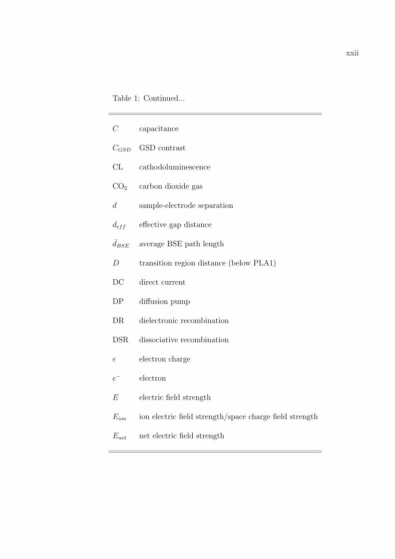
Table 1: Continued...
C capacitance
CGSD GSD contrast
CL cathodoluminescence
CO2 carbon dioxide gas
d sample-electrode separation
deff effective gap distance
dBSE average BSE path length
D transition region distance (below PLA1)
DC direct current
DP diffusion pump
DR dielectronic recombination
DSR dissociative recombination
e electron charge
e− electron
E electric field strength
Eion ion electric field strength/space charge field strength
Enet net electric field strength
Page 24
xxiii
Table 1: Continued...
EGSED GSED electric field strength
E/p reduced electric field
EBIC electron beam induced current
EC environmental chamber
ESE environmental secondary electron
ESEM environmental scanning electron microscope
E-T Everhart-Thornley
fe(θ) scattering amplitude
FET field effect transistor
gm metastable geometrical loss factor
gp photon geometrical loss factor
GPMT PMT gain
GSD gaseous scintillation detector
GSED gaseous secondary electron detector
GSI greyscale intensity
h Planks constant
h transition region distance (above PLA1)
Page 25
xxiv
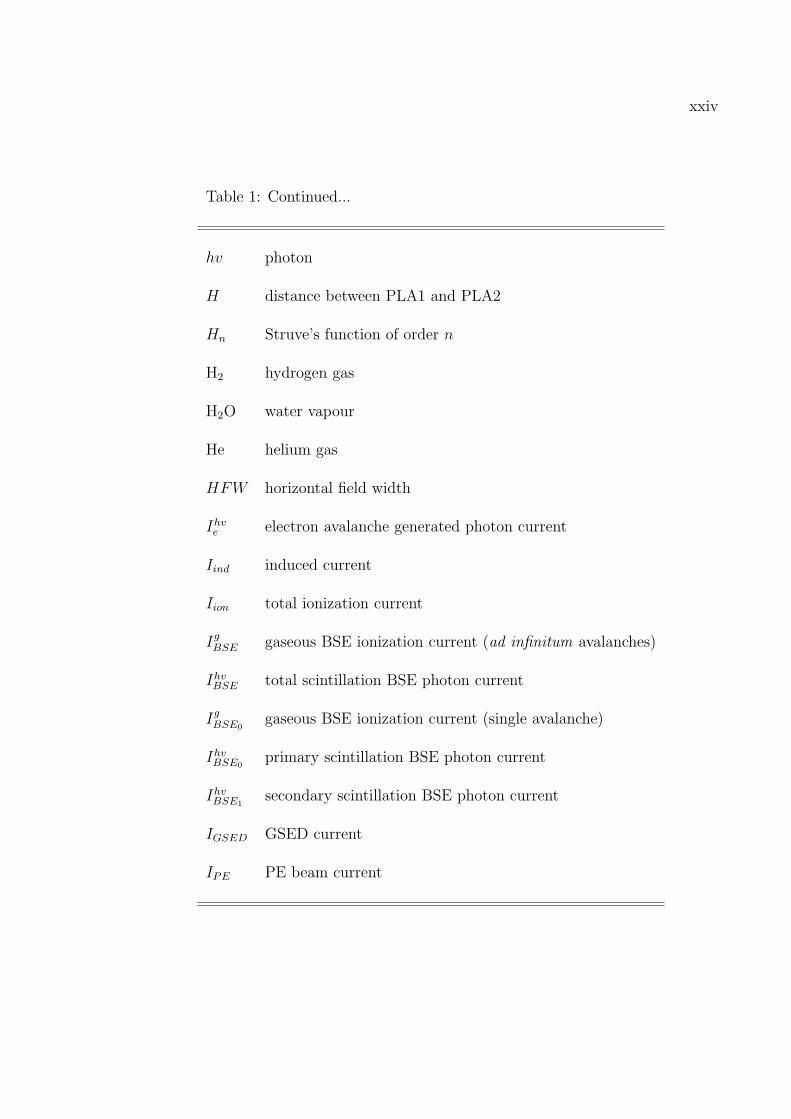
Table 1: Continued...
hv photon
H distance between PLA1 and PLA2
Hn Struve’s function of order n
H2 hydrogen gas
H2O water vapour
He helium gas
HFW horizontal field width
Ihve electron avalanche generated photon current
Iind induced current
Iion total ionization current
IgBSE gaseous BSE ionization current (ad infinitum avalanches)
IhvBSE total scintillation BSE photon current
IgBSE0
gaseous BSE ionization current (single avalanche)
IhvBSE0
primary scintillation BSE photon current
IhvBSE1
secondary scintillation BSE photon current
IGSED GSED current
IPE PE beam current
Page 26
xxv
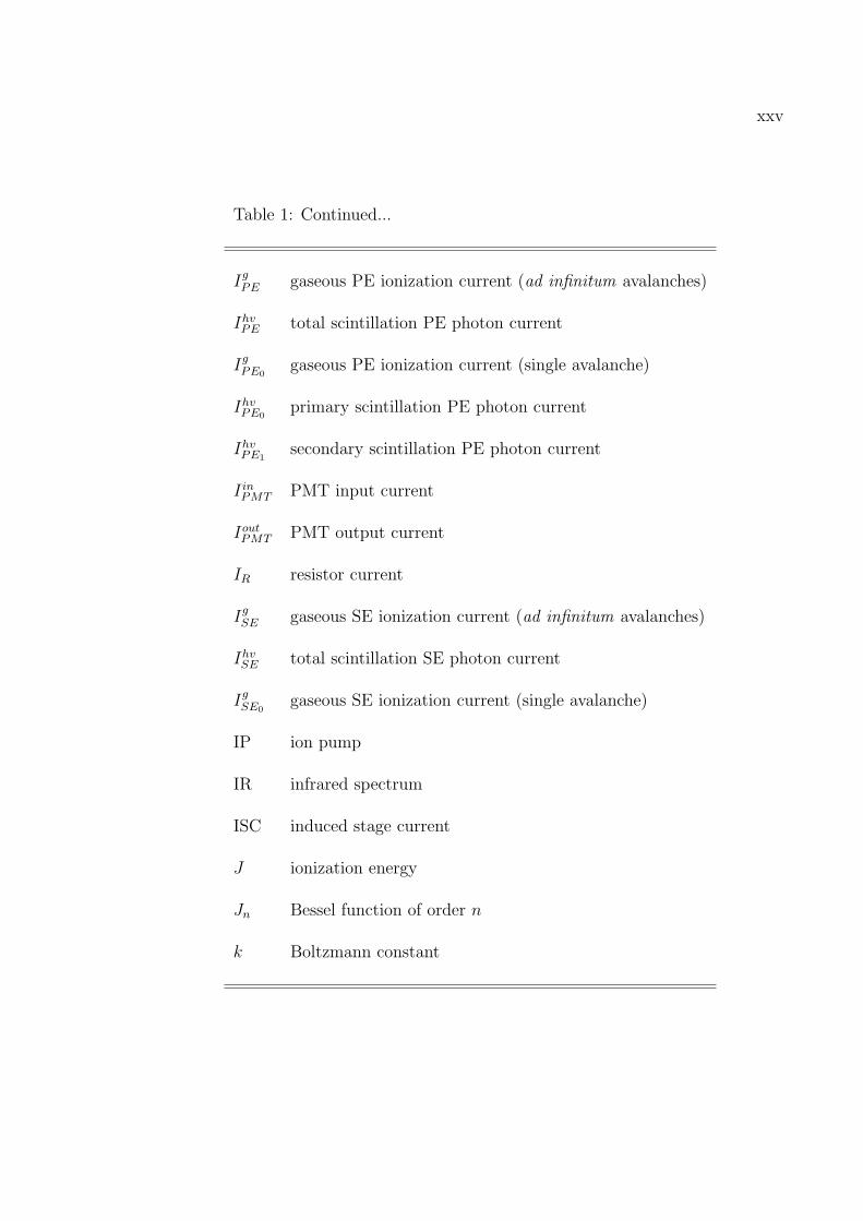
Table 1: Continued...
IgPE gaseous PE ionization current (ad infinitum avalanches)
IhvPE total scintillation PE photon current
IgPE0
gaseous PE ionization current (single avalanche)
IhvPE0
primary scintillation PE photon current
IhvPE1
secondary scintillation PE photon current
I inPMT PMT input current
IoutPMT PMT output current
IR resistor current
IgSE gaseous SE ionization current (ad infinitum avalanches)
IhvSE total scintillation SE photon current
IgSE0
gaseous SE ionization current (single avalanche)
IP ion pump
IR infrared spectrum
ISC induced stage current
J ionization energy
Jn Bessel function of order n
k Boltzmann constant
Page 27
xxvi
Table 1: Continued...
k cascade amplification feedback factor
K kinetic energy
Ki ion kinetic energy
Kn neutral atom/molecule kinetic energy
KSE SE kinetic energy
K0 modified Bessel function of the second kind of zero order
L dimensional unit of length
LED light emitting diode
m average number of scattering events
me electron rest mass
M metastable-cathodic electron emission probability
M molecule
MGSI mean greyscale intensity
n number density/concentration
ne electron number density/concentration
ni ion number density/concentration
N ce number of cathodic electrons
Page 28
xxvii
Table 1: Continued...
N ge number of gaseous electrons
N ghv number of gaseous photons
Nn Neumann’s Bessel function of the second kind of order n
N cp number of cathodic photoelectrons
NhvBSE number of photons generated by BSEs
NhvCL number of photons generated by CL
NhvPE number of photons generated by PEs
NhvSE number of photons generated by SEs
NhvT total number of photons
N2 nitrogen gas
NO nitrous oxide gas
O2 oxygen gas
p pressure
pmax maximum efficiency pressure
pemax maximum ionization efficiency pressure
phvmax maximum excitation efficiency pressure
pAr argon pressure
Page 29
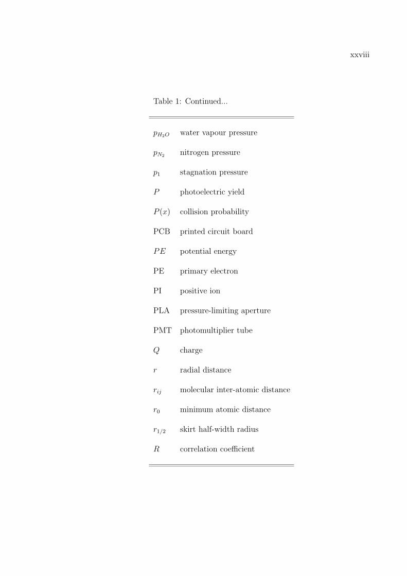
xxviii
Table 1: Continued...
pH2O water vapour pressure
pN2 nitrogen pressure
p1 stagnation pressure
P photoelectric yield
P (x) collision probability
PCB printed circuit board
PE potential energy
PE primary electron
PI positive ion
PLA pressure-limiting aperture
PMT photomultiplier tube
Q charge
r radial distance
rij molecular inter-atomic distance
r0 minimum atomic distance
r1/2 skirt half-width radius
R correlation coefficient
Page 30
xxix
Table 1: Continued...
R effective atomic radius
R resistance
Rm maximum electron interaction range
RL load resistance
RS series resistance
RC time constant
RCnf noise filter time constant
RDR radiative dielectronic recombination
RE resonant excitation
RP rotary pump
RR radiative recombination
s particle displacement
ske(λ)p photocathode spectral sensitivity
SBSE BSE ionization efficiency
SPE PE ionization efficiency
SbKCs Bailkaline
(S/B)SE SE signal-to-background ratio
Page 31
xxx
Table 1: Continued...
(S/B)eSE electronic SE signal-to-background ratio
(S/B)hvSE electroluminescent SE signal-to-background ratio
SE secondary electron
SEM scanning electron microscope
SNR signal-to-noise ratio
t time
T absolute temperature
T dimensional unit of time
TBR three-body recombination
TV television
T (λ) transmission response
UV ultra violet spectrum
v photon frequency
vc critical photon frequency
ve electron drift velocity
ve average electron velocity
vi ion drift velocity
Page 32
xxxi
Table 1: Continued...
V voltage
V 1e first excitation potential
V 1i first ionization potential
Vp(ρ) plural scattering probability distribution
Vs(r) single scattering probability distribution
VGSD GSD voltage
VGSED GSED voltage
VHT PMT high tension voltage
V outPMT PMT output voltage
VS voltage signal
VIS visible spectrum
VPSEM variable pressure scanning electron microscope
VUV vacuum ultra violet spectrum
WD working distance
z gap distance
zΩ maximum SE-ion recombination distance
Z atomic number
Page 33
xxxii
Table 1: Continued...
αexc excitation coefficient
αion first Townsend ionization coefficientSE/ESE ionization efficiency
αswion first Townsend ionization coefficient
SE/ESE ionization efficiency (swarm conditions)
γ total second Townsend coefficient
γi ion second Townsend coefficient
γm metastable second Townsend coefficient
γn neutral atom/molecule second Townsend coefficient
γp photoelectron second Townsend coefficient
Γe electron transit time
Γi ion transit time
δ SE emission coefficient
δeff effective SE emission coefficient
∆ reaction by-products
ε electron energy
εBSE BSE energy
εPE PE energy
εSE average SE energy
ε0 electron rest energy
Page 34
xxxiii
Table 1: Continued...
ζT mass thickness of transition region
ζ(t) SE-ion recombination rate
η BSE emission coefficient
θ scattering angle
λ photon wavelength
λc critical photon wavelength
λe relativistic electron wavelength
λSE SE inelastic mean free path
λeSE SE mean free path (ionization)
λhvSE SE mean free path (excitation)
λ1 minimum photon wavelength
λ2 maximum photon wavelength
µm metastable absorption coefficient
µp photon absorption coefficient
ρ reduced radial distance
ρ total SE-ion recombination coefficient
ρDSR SE-ion recombination coefficient (DSR)
ρRR SE-ion recombination coefficient (RR)
Page 35
xxxiv
Table 1: Continued...
σse elastic scattering cross section
σsi inelastic scattering cross section
σiT total electron impact ionization cross section
σeiT total electron-ion recombination cross section
σsT total scattering cross section
τi average ion lifetime
τmin minimum greyscale intensity time
τp pixel dwell time
τL line scan time
υ fraction of SEs escaping back diffusion
Φ work function
Φhv(λ) radiant photon flux
χ metastable coefficient
ψ ionization rate
ωBSE BSE excitation efficiency
ωPE PE excitation efficiency
Ω scattering solid angle
Ω average SE-ion capture probability
Page 36
Abstract
This thesis quantitatively investigates gaseous electron-ion recombination in an envi-
ronmental scanning electron microscope (ESEM) at a transient level by utilizing the
dark shadows/streaks seen in gaseous secondary electron detector (GSED) images
immediately after a region of enhanced secondary electron (SE) emission is encoun-
tered by a scanning electron beam. The investigation firstly derives a theoretical
model of gaseous electron-ion recombination that takes into consideration transients
caused by the time constant of the GSED electronics and external circuitry used to
generate images. Experimental data of pixel intensity versus time of the streaks is
then simulated using the model enabling the relative magnitudes of (i) ionization and
recombination rates, (ii) recombination coefficients, and (iii) electron drift velocities,
as well as absolute values of the total time constant of the detection system, to be
determined as a function of microscope operating parameters. Results reveal the
exact dependence that the effects of SE-ion recombination on signal formation have
on reduced electric field intensity and time in ESEM. Furthermore, the model im-
plicitly demonstrates that signal loss as a consequence of field retardation due to ion
space charges, although obviously present, is not the foremost phenomenon causing
streaking in images, as previously thought.
Following that the generation and detection of gaseous scintillation and electro-
luminescence produced via electron-gas molecule excitation reactions in ESEM is
investigated. Here a novel gaseous scintillation detection (GSD) system is developed
xxxv
Page 37
xxxvi
to efficiently detect photons produced. Images acquired using GSD are compared
to those obtained using conventional GSED detection, and demonstrate that images
rich in SE contrast can be achieved using such systems. A theoretical model is devel-
oped that describes the generation of photon signals by cascading SEs, high energy
backscattered electrons (BSEs) and primary beam electrons (PEs). Photon amplifi-
cation, or the total number of photons produced per sample emissive electron, is then
investigated, and compared to conventional electronic amplification, over a wide range
of microscope operating parameters, imaging gases and photon collection geometries.
The main findings of the investigation revealed that detected electroluminescent sig-
nals exhibit larger SE signal-to-background levels than that of conventional electronic
signals detected via GSED. Also, dragging the electron cascade towards the light pipe
assemblage of GSD systems, or electrostatic focusing, dramatically increases photon
collection efficiencies. The attainment of such an improvement being a direct conse-
quence of increasing the ‘effective’ solid angle for photon collection.
Finally, in attempt to characterize the scintillating wavelengths arising from sam-
ple emissive SEs, PEs, BSEs, and their respective cascaded electrons, such that future
photon filtering techniques can be employed to extract nominated GSD imaging sig-
nals, the emission spectra of commonly utilized electroluminescent gases in ESEM,
such as argon (Ar) and nitrogen (N2), were collected and investigated. Spectra of Ar
and N2 reveal several major emission lines that occur in the ultraviolet (UV) to near-
infrared (NIR) regions of the electromagnetic spectrum. The major photon emissions
discovered in Ar are attributed to occur via atomic de-excitation transitions of neutral
Ar (Ar I), whist for N2, major emissions are attributed to be a consequence of second
positive band vibrational de-excitation reactions. Major wavelength intensity versus
gas pressure data, for both Ar and N2, illustrate that wavelength intensities increase
with decreasing pressure. This phenomenon strongly suggesting that quenching ef-
fects and reductions in excitation mean free paths increase with imaging gas pressure.


![2SHUDWLRQRIWKH=HUR,RQ%DFNIORZHOHFWURQ … · 2019-05-25 · The development of micro-patterned gaseous electron multipliers such as the Gas Electron Multiplier (GEM) [4], Micromegas](https://static.documents.pub/doc/80x56/5e46f41ecb54f851eb09ed28/2shudwlrqriwkhhurrqdfniorzhohfwurq-2019-05-25-the-development-of-micro-patterned.jpg)


