ECG 740

GENERATION SCHEDULING (UNIT COMMITMENT)

1

Unit Commitment

• Given a load profile, e.g., values of the load for each hour of a day.

• Given set of units available,

• When should each unit be started, stopped and how much should it generate to meet the load at minimum cost?

2

G G G Load Profile

? ? ?

Load

Time 12 6 0 18 24

500

1000

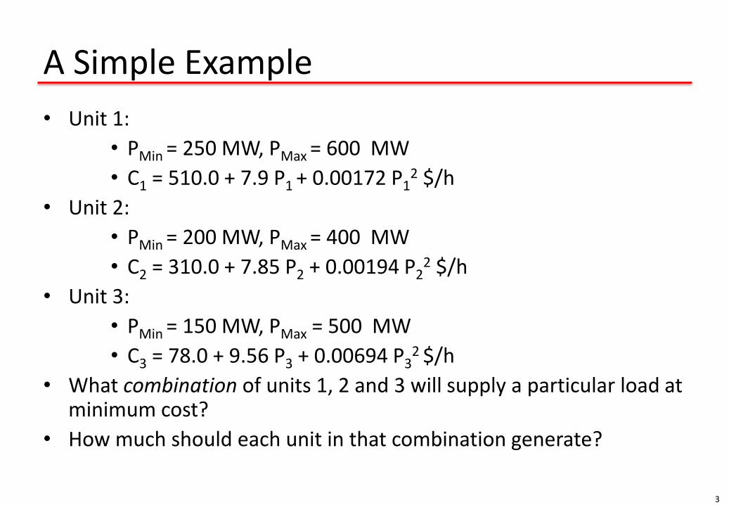
A Simple Example

• Unit 1:

• PMin = 250 MW, PMax = 600 MW

• C1 = 510.0 + 7.9 P1 + 0.00172 P12 $/h

• Unit 2:

• PMin = 200 MW, PMax = 400 MW

• C2 = 310.0 + 7.85 P2 + 0.00194 P22 $/h

• Unit 3:

• PMin = 150 MW, PMax = 500 MW

• C3 = 78.0 + 9.56 P3 + 0.00694 P32 $/h

• What combination of units 1, 2 and 3 will supply a particular load at minimum cost?

• How much should each unit in that combination generate?

3

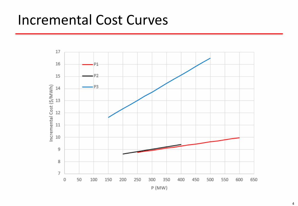
Incremental Cost Curves

4

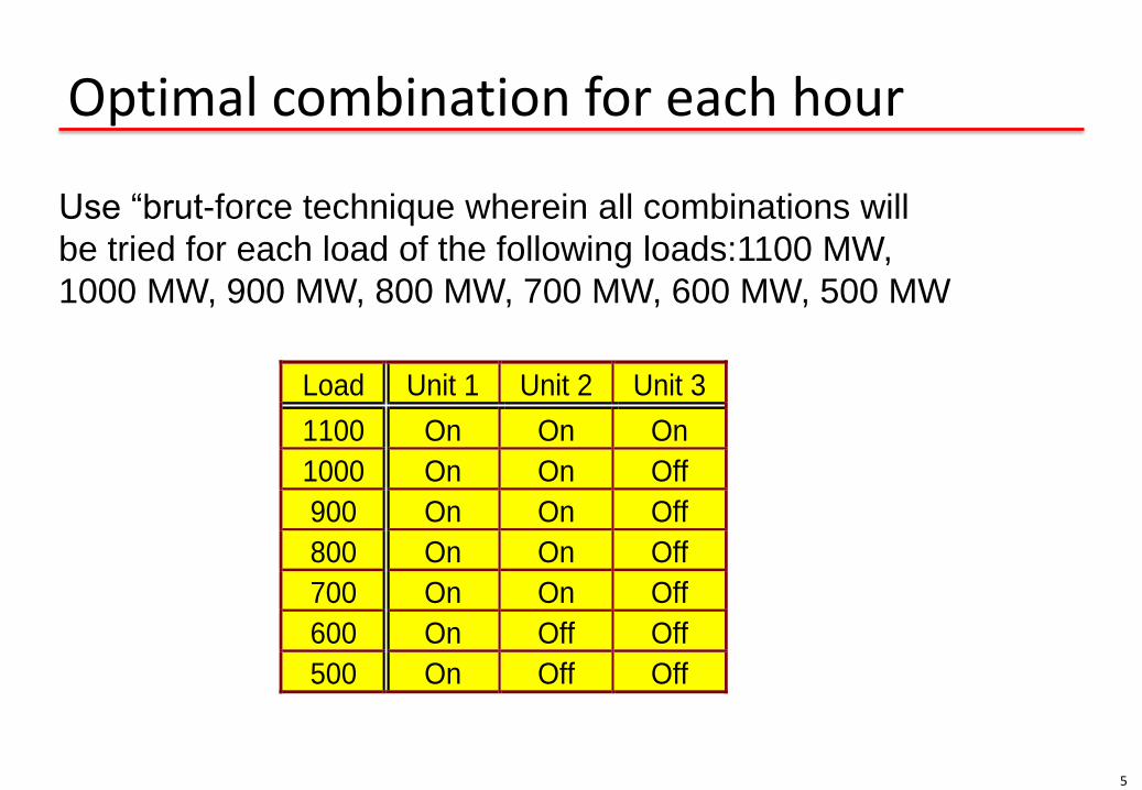
Optimal combination for each hour

Load Unit 1 Unit 2 Unit 3

1100 On On On

1000 On On Off

900 On On Off

800 On On Off

700 On On Off

600 On Off Off

500 On Off Off

5

Use “brut-force technique wherein all combinations will

be tried for each load of the following loads:1100 MW,

1000 MW, 900 MW, 800 MW, 700 MW, 600 MW, 500 MW

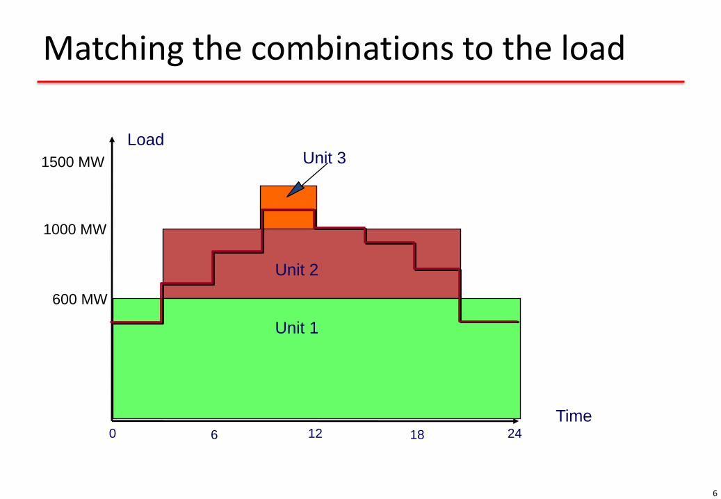
Matching the combinations to the load

6

Load

Time 12 6 0 18 24

Unit 1

Unit 2

Unit 3

600 MW

1000 MW

1500 MW

Issues that must be considered

• Constraints

– Unit constraints

– System constraints

• Some constraints create a link between periods

• Start-up costs

– Cost incurred when we start a generating unit

– Different units have different start-up costs

• Curse of dimensionality

7

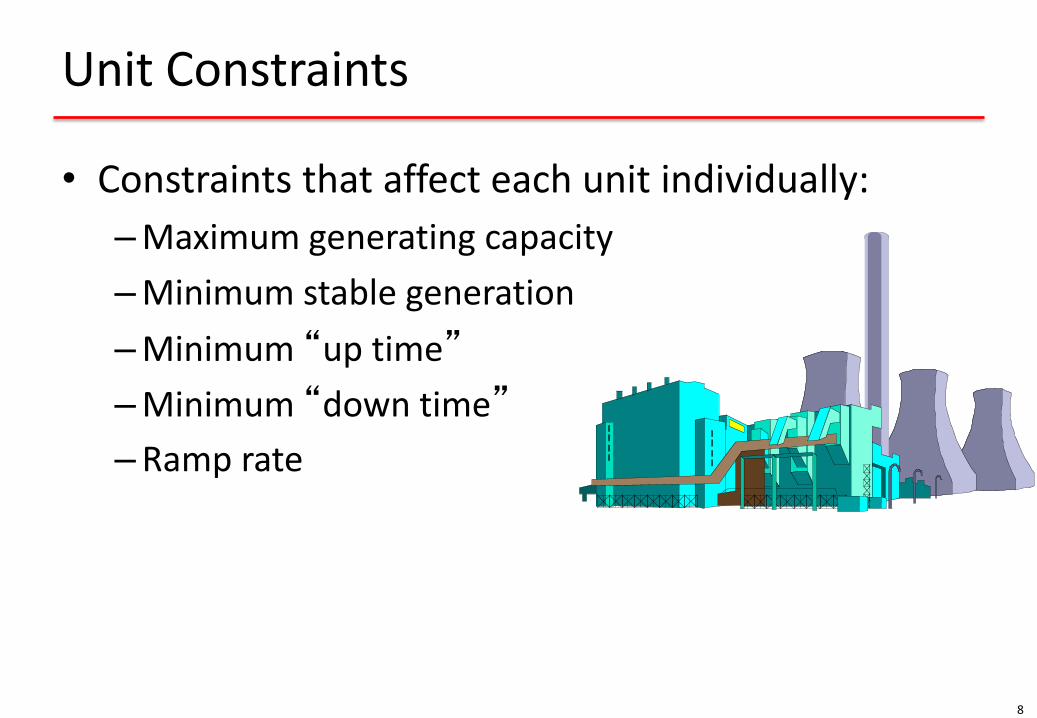
Unit Constraints

• Constraints that affect each unit individually:

–Maximum generating capacity

–Minimum stable generation

–Minimum “up time”

–Minimum “down time”

–Ramp rate

8

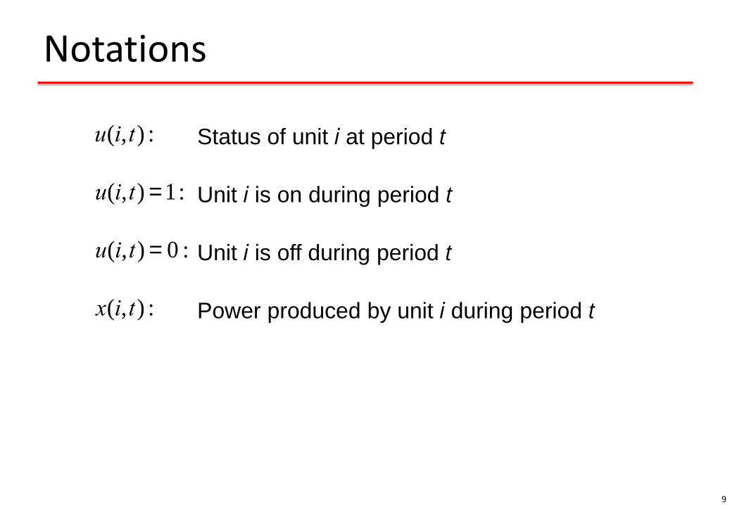
Notations

9

u(i,t) : Status of unit i at period t

x(i,t) : Power produced by unit i during period t

Unit i is on during period t u(i,t) = 1:

Unit i is off during period t u(i,t) = 0 :

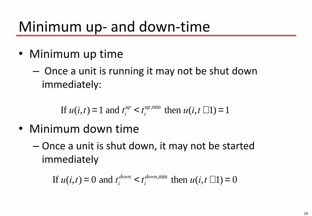
Minimum up- and down-time

• Minimum up time

– Once a unit is running it may not be shut down immediately:

• Minimum down time

– Once a unit is shut down, it may not be started immediately

10

If u(i,t) = 1 and tiup < ti

up,min then u(i,t +1) = 1

If u(i,t) = 0 and tidown < ti

down,min then u(i,t +1) = 0

Ramp rates

• Maximum ramp rates

– To avoid damaging the turbine, the electrical output of a unit cannot change by more than a certain amount over a period of time:

11

x i,t +1( ) - x i,t( ) £ DPiup,max

x(i,t)- x(i,t +1) £ DPidown,max

Maximum ramp up rate constraint:

Maximum ramp down rate constraint:

System Constraints

• Constraints that affect more than one unit

– Load/generation balance

– Reserve generation capacity

– Emission constraints

– Network constraints

12

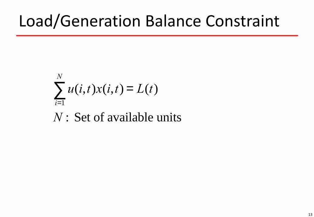
Load/Generation Balance Constraint

13

u(i,t)x(i,t)i=1

N

å = L(t)

N : Set of available units

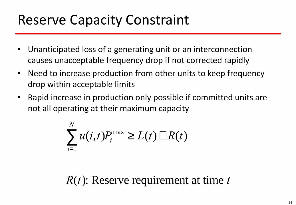
Reserve Capacity Constraint

• Unanticipated loss of a generating unit or an interconnection causes unacceptable frequency drop if not corrected rapidly

• Need to increase production from other units to keep frequency drop within acceptable limits

• Rapid increase in production only possible if committed units are not all operating at their maximum capacity

14

u(i,t)i=1

N

å Pimax ³ L(t) + R(t)

R(t): Reserve requirement at time t

Cost of Reserve

• Reserve has a cost even when it is not called

• More units scheduled than required

– Units not operated at their maximum efficiency

– Extra start up costs

• Must build units capable of rapid response

• Cost of reserve proportionally larger in small systems

• Important driver for the creation of interconnections between systems

15

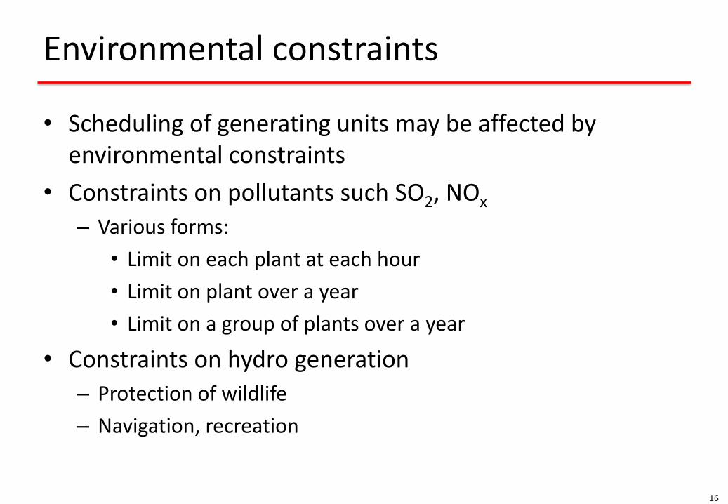
Environmental constraints

• Scheduling of generating units may be affected by environmental constraints

• Constraints on pollutants such SO2, NOx

– Various forms:

• Limit on each plant at each hour

• Limit on plant over a year

• Limit on a group of plants over a year

• Constraints on hydro generation

– Protection of wildlife

– Navigation, recreation

16

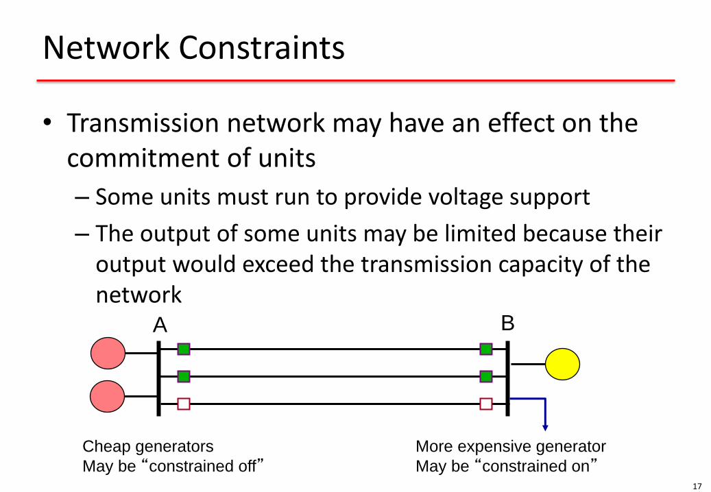
Network Constraints

• Transmission network may have an effect on the commitment of units

– Some units must run to provide voltage support

– The output of some units may be limited because their output would exceed the transmission capacity of the network

17

Cheap generators

May be “constrained off” More expensive generator

May be “constrained on”

A B

Start-up Costs

• Thermal units must be “warmed up” before they can be brought on-line

• Warming up a unit costs money

• Start-up cost depends on time unit has been off

18

SCi (t iOFF ) = a i + b i (1 - e

-tiOFF

t i )

tiOFF

αi

αi + βi

Start-up Costs

• Need to “balance” start-up costs and running costs

• Example: – Diesel generator: low start-up cost, high running cost

– Coal plant: high start-up cost, low running cost

• Issues: – How long should a unit run to “recover” its start-up cost?

– Start-up one more large unit or a diesel generator to cover the peak?

– Shutdown one more unit at night or run several units part-loaded?

19

Summary

• Some constraints link periods together

• Minimizing the total cost (start-up + running) must be done over the whole period of study

• Generation scheduling or unit commitment is a more general problem than economic dispatch

• Economic dispatch is a sub-problem of generation scheduling

20

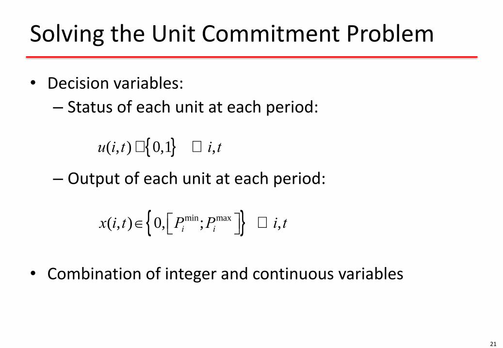
Solving the Unit Commitment Problem

• Decision variables:

– Status of each unit at each period:

– Output of each unit at each period:

• Combination of integer and continuous variables

21

u(i,t) Î 0,1{ }   " i,t

x(i,t)Î 0, Pimin;Pi

maxéë ùû{ }  " i,t

Optimization with integer variables

• Continuous variables – Can follow the gradients or use LP

– Any value within the feasible set is OK

• Discrete variables – There is no gradient

– Can only take a finite number of values

– Problem is not convex

– Must try combinations of discrete values

22

How many combinations are there?

23

• Examples

– 3 units: 8 possible states

– N units: 2N possible states

111

110

101

100

011

010

001

000

How many solutions are there?

© 2011 Daniel Kirschen and the University of Washington 24

1 2 3 4 5 6 T=

• Optimization over a time horizon divided into intervals

• A solution is a path linking one combination at each interval

• How many such paths are there?

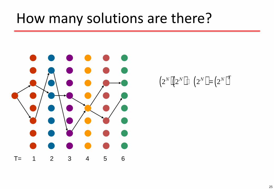
How many solutions are there?

25

1 2 3 4 5 6 T=

2N( ) 2N( )… 2N( ) = 2N( )T

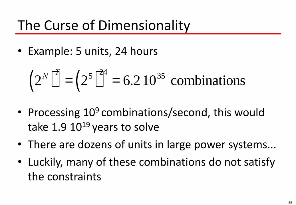
The Curse of Dimensionality

• Example: 5 units, 24 hours

• Processing 109 combinations/second, this would take 1.9 1019 years to solve

• There are dozens of units in large power systems...

• Luckily, many of these combinations do not satisfy the constraints

26

2N( )T

= 25( )24

= 6.2 1035 combinations

How do you Beat the Curse?

Brute force approach won’t work!

• Need to be smart

• Try only a small subset of all combinations

• Can’t guarantee optimality of the solution

• Try to get as close as possible within a reasonable amount of time

27

Main Solution Techniques

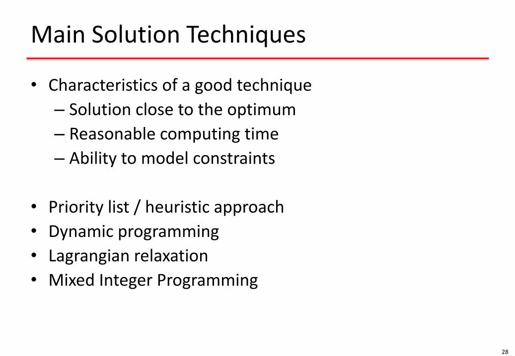
• Characteristics of a good technique

– Solution close to the optimum

– Reasonable computing time

– Ability to model constraints

• Priority list / heuristic approach

• Dynamic programming

• Lagrangian relaxation

• Mixed Integer Programming

28

Priority List Method

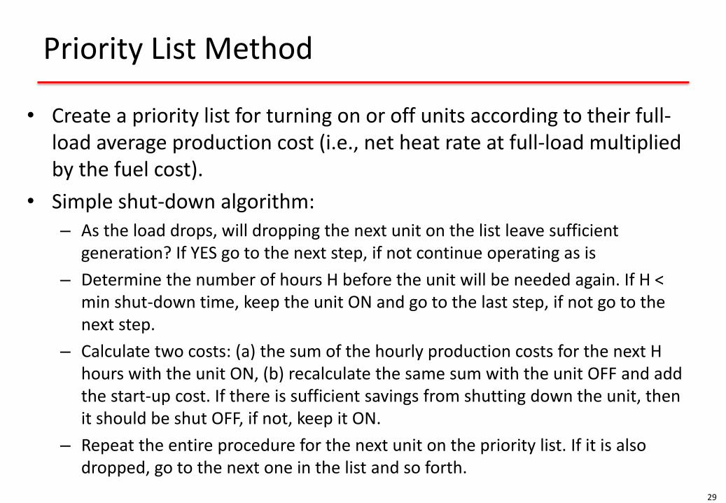
• Create a priority list for turning on or off units according to their full-load average production cost (i.e., net heat rate at full-load multiplied by the fuel cost).

• Simple shut-down algorithm: – As the load drops, will dropping the next unit on the list leave sufficient

generation? If YES go to the next step, if not continue operating as is

– Determine the number of hours H before the unit will be needed again. If H < min shut-down time, keep the unit ON and go to the last step, if not go to the next step.

– Calculate two costs: (a) the sum of the hourly production costs for the next H hours with the unit ON, (b) recalculate the same sum with the unit OFF and add the start-up cost. If there is sufficient savings from shutting down the unit, then it should be shut OFF, if not, keep it ON.

– Repeat the entire procedure for the next unit on the priority list. If it is also dropped, go to the next one in the list and so forth.

29

Dynamic Programming

• Dynamic Programming (DP) is an algorithm for optimization problems.

• DP solves problems by combining solutions of subproblems.

• Subproblems are not independent. – Subproblems may share subsubproblems,

• DP reduces computation by – Solving subproblems in a forward or backward fashion.

– Storing solution to a subproblem the first time it is solved.

– Looking up the solution when subproblem is encountered again.

• Key: determine the structure of optimal solutions

Dynamic Programming Algorithm

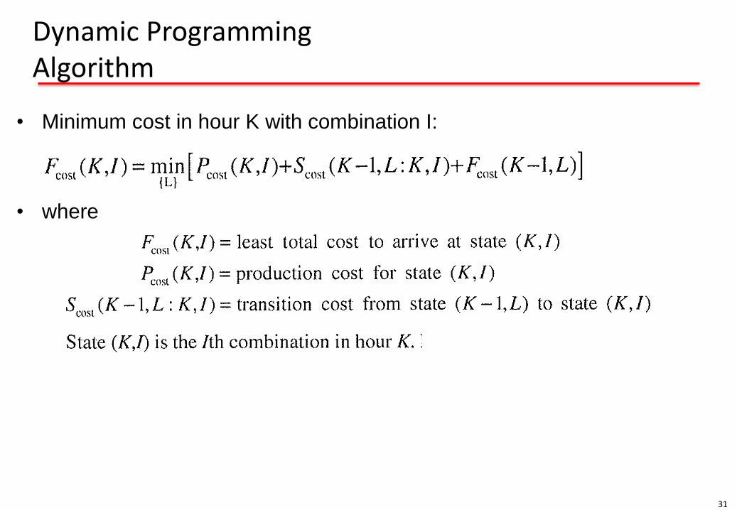
• Minimum cost in hour K with combination I:

• where

31

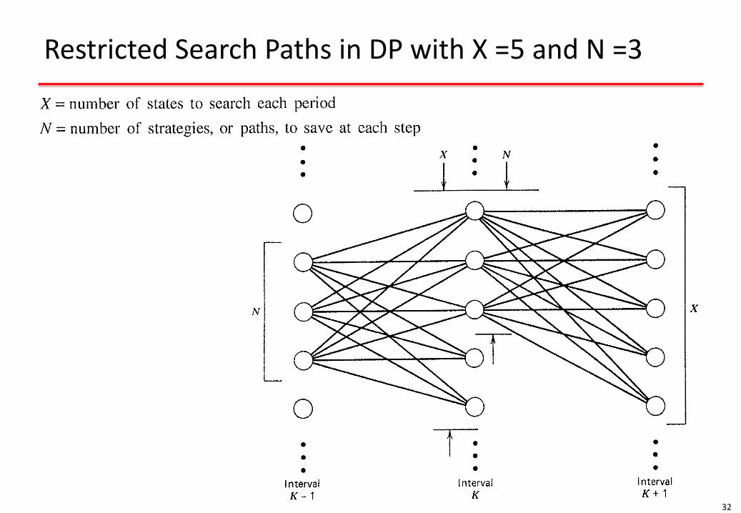
Restricted Search Paths in DP with X =5 and N =3

32

Dynamic Programming Algorithm

33

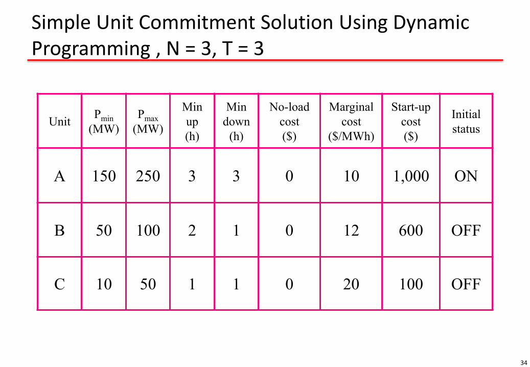
Simple Unit Commitment Solution Using Dynamic Programming , N = 3, T = 3

34

Unit Pmin

(MW)

Pmax

(MW)

Min

up

(h)

Min

down

(h)

No-load

cost

($)

Marginal

cost

($/MWh)

Start-up

cost

($)

Initial

status

A 150 250 3 3 0 10 1,000 ON

B 50 100 2 1 0 12 600 OFF

C 10 50 1 1 0 20 100 OFF

Demand Data

35

Hourly Demand

0

50

100

150

200

250

300

350

1 2 3

Hours

Load

Reserve requirements are not considered

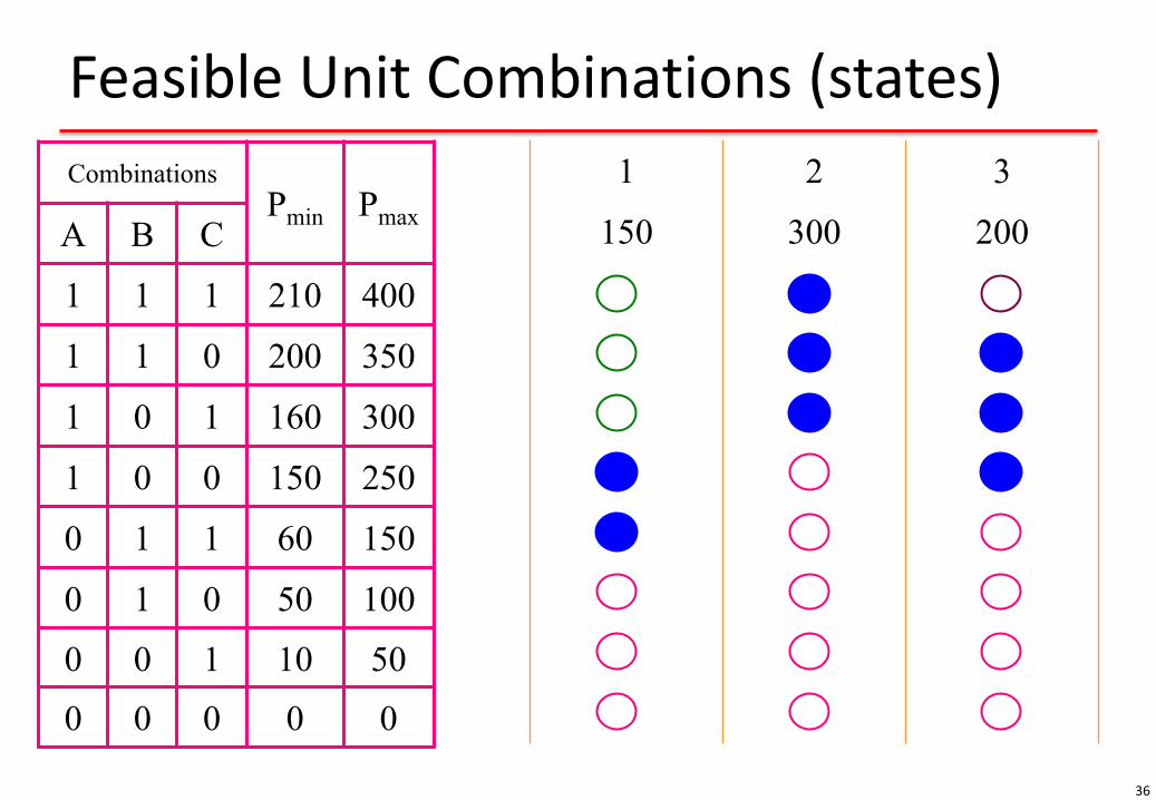
Feasible Unit Combinations (states)

36

Combinations

Pmin Pmax A B C

1 1 1 210 400

1 1 0 200 350

1 0 1 160 300

1 0 0 150 250

0 1 1 60 150

0 1 0 50 100

0 0 1 10 50

0 0 0 0 0

1 2 3

150 300 200

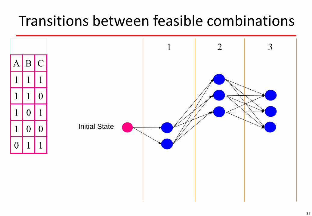
Transitions between feasible combinations

37

A B C

1 1 1

1 1 0

1 0 1

1 0 0

0 1 1

1 2 3

Initial State

Infeasible transitions: Minimum down time of unit A

38

A B C

1 1 1

1 1 0

1 0 1

1 0 0

0 1 1

1 2 3

Initial State

TD TU

A 3 3

B 1 2

C 1 1

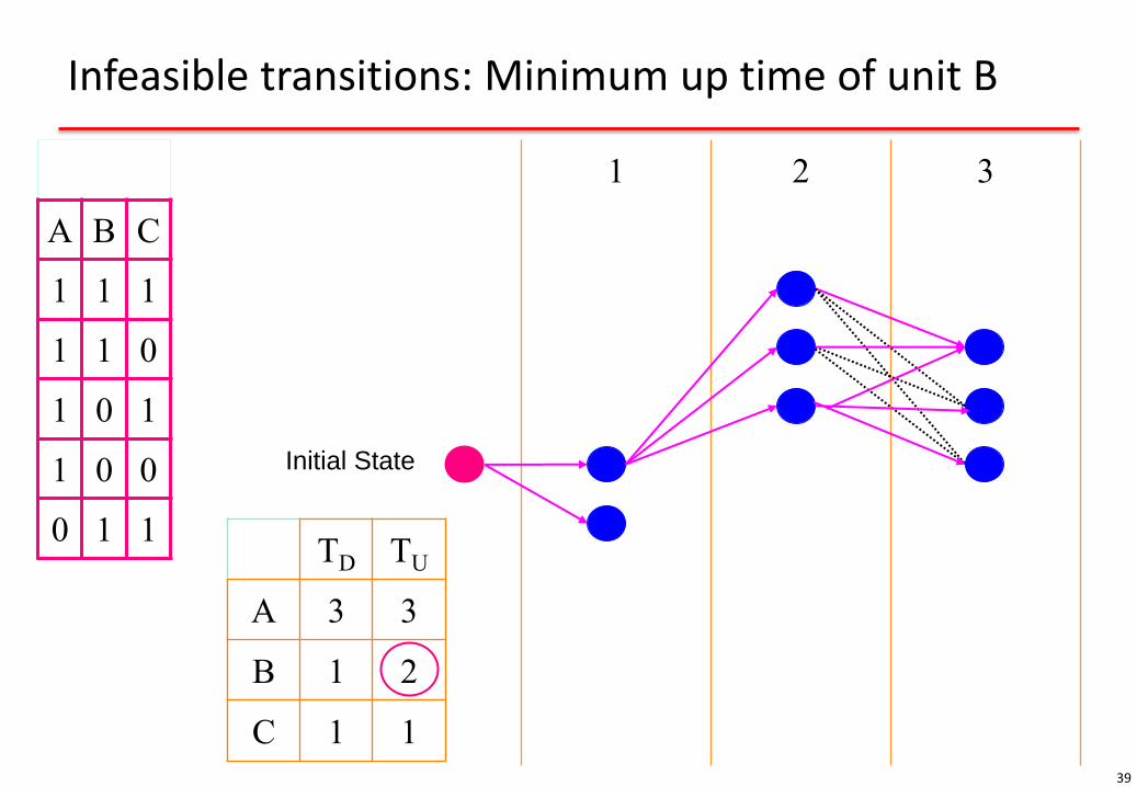
Infeasible transitions: Minimum up time of unit B

39

A B C

1 1 1

1 1 0

1 0 1

1 0 0

0 1 1

1 2 3

Initial State

TD TU

A 3 3

B 1 2

C 1 1

Feasible transitions

40

A B C

1 1 1

1 1 0

1 0 1

1 0 0

0 1 1

1 2 3

Initial State

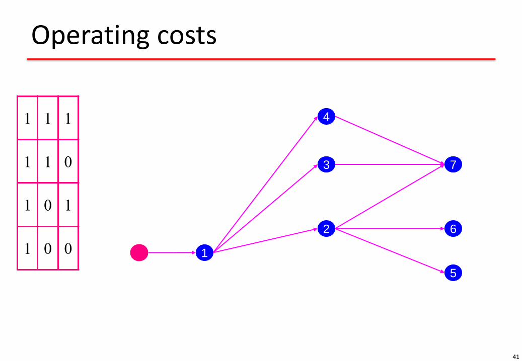
Operating costs

41

1 1 1

1 1 0

1 0 1

1 0 0 1

4

3

2

5

6

7

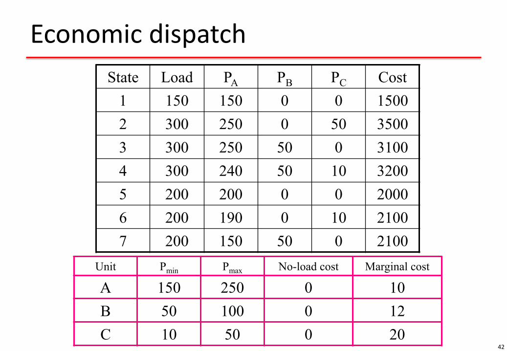
Economic dispatch

42

State Load PA PB PC Cost

1 150 150 0 0 1500

2 300 250 0 50 3500

3 300 250 50 0 3100

4 300 240 50 10 3200

5 200 200 0 0 2000

6 200 190 0 10 2100

7 200 150 50 0 2100

Unit Pmin Pmax No-load cost Marginal cost

A 150 250 0 10

B 50 100 0 12

C 10 50 0 20

Operating costs

43

1 1 1

1 1 0

1 0 1

1 0 0 1

4

3

2

5

6

7

$1500

$3500

$3100

$3200

$2000

$2100

$2100

Start-up costs

44

1 1 1

1 1 0

1 0 1

1 0 0 1

4

3

2

5

6

7

$1500

$3500

$3100

$3200

$2000

$2100

$2100

Unit Start-up cost

A 1000

B 600

C 100

$0

$0

$0

$0

$0

$600

$100

$600

$700

Accumulated costs

45

1 1 1

1 1 0

1 0 1

1 0 0 1

4

3

2

5

6

7

$1500

$3500

$3100

$3200

$2000

$2100

$2100

$1500

$5100

$5200

$5400

$7300

$7200

$7100 $0

$0

$0

$0

$0

$600

$100

$600

$700

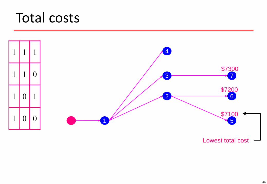
Total costs

46

1 1 1

1 1 0

1 0 1

1 0 0 1

4

3

2

5

6

7

$7300

$7200

$7100

Lowest total cost

Optimal solution

47

1 1 1

1 1 0

1 0 1

1 0 0 1

2

5

$7100

Notes

• This example is intended to illustrate the principles of unit commitment

• Some constraints have been ignored and others artificially tightened to simplify the problem and make it solvable by hand

• Therefore it does not illustrate the true complexity of the problem

• The solution method used in this example is based on dynamic programming. This technique works well for systems with < 20 units.

48

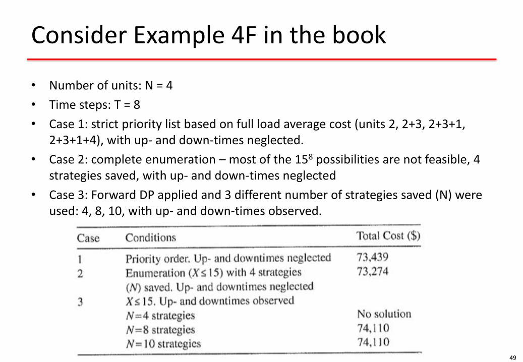
Consider Example 4F in the book

• Number of units: N = 4

• Time steps: T = 8

• Case 1: strict priority list based on full load average cost (units 2, 2+3, 2+3+1, 2+3+1+4), with up- and down-times neglected.

• Case 2: complete enumeration – most of the 158 possibilities are not feasible, 4 strategies saved, with up- and down-times neglected

• Case 3: Forward DP applied and 3 different number of strategies saved (N) were used: 4, 8, 10, with up- and down-times observed.

49