11524 Clear Creek Place, Boca Raton, FL 33428-2413: [email protected]
Gray Line Propagation, or Florida to Cocos (Keeling) on 80 m
N4II investigates mechanisms reponsible for gray line propagation on the low bands.
IntroductionFrom 30 March to 13 April 2013, Chris
Tran, GM3WOJ, and Keith Kerr, GM4YXI, operated as VK9CZ from the Cocos (Keeling) Islands, the DXCC entity farthest from my location in south Florida. When this DXpedition was announced in late 2012, I determined that I wanted to work VK9CZ on 80 m.
The first step was to identify the period of common darkness between us — if, in fact, one existed. A check of the sunrise (SR) and sunset (SS) times at both locations for 7 April, midway through the DXpedition, revealed the following:
VK9CZ SS = 1132Z; N4II SR = 1106ZVK9CZ SR = 2337Z; N4II SS = 2340Z.There was no period of mutual darkness,
but I thought that the low bands might still be
a possibility at the “gray line” of my SS and VK9CZ SR, which occurred within three minutes of each other. In the past I had heard stories of enhanced propagation under such conditions from grizzled low-band veterans, and I was curious to find out if I could hear VK9CZ on 80 m at all.
Due to CC&R restrictions at my home, I chose to operate from nearby club stations. The best 80 m station available at the time was at the Boca Raton Amateur Radio Association, N4BRF. It offered a SteppIR vertical, with 60 radials, in a quiet location on the edge of the Loxahatchee National Wildlife Refuge, and a 500 W transmit power amplifier. The station did not have a dedicated receive antenna.
My first opportunity was on 3 April. Not knowing what to expect, I began monitoring 80 m CW at 2300Z (40 minutes before my
SS). At 2325Z, to my delight I heard VK9CZ calling CQ on 3507.5 kHz. There was no pile-up, and he was not working split. To my amazement I worked him on the first call, as N4II. He called CQ again and, still with no pile-up, I worked him again, this time using the club call sign N4BRF. VK9CZ called CQ again and again, until he finally faded at 2345 Z — 5 minutes after my SS, and 8 minutes after his SR. The next 80 m opportunity was on 5 April, but a large thunderstorm sat over the club station, keeping me off the air.
On 7 April, wanting to hear more, I began monitoring 80 m CW at 2315Z, 25 minutes before SS. At 2330Z, I heard VK9CZ again calling CQ on 3507.5 kHz. There still was no true pile-up. He worked several stations in an orderly, workmanlike fashion before fading at 2350Z, 10 minutes after my SS, and 13 minutes after his SR.
QX1611-Callaway01
VK9CZ
N4BRF
Figure 1 — Into daylight? Some reports indicated that the received VK9CZ signal peaked to the SSW. [DX Atlas]
This experience left me stunned. Why no pileup? Why so strong? How could he be worked almost at will, from 11,450 miles away, on 80 m? Where was everyone else?
What kind of propagation made this possible?
The InvestigationMy curiosity probably would have stayed
idle, were it not for an item that appeared in the ARRL Propagation Bulletin the following week on 12 April. Bruce Smith, AC4G, wrote in to say:
“I was so excited to QSO VK9CZ on 80 m CW that I had to write in. Our QSO took place on 3 April around 2345Z when VK9CZ and my location in southern Tennessee were in sunlight
at the edge of the terminator. This had to be one of my best QSOs ever due to the level of difficulty, the distance, and no darkness at either location (so my terminator map showed).
The VK9CZ signal was S5-S7 on my transmit antenna (vertical). The signal was so strong that my separate receive antenna was not required. Since that date, I have not been able to copy their 80 m signal. I guess it was one of my luckiest days to be able to make this QSO.”Well! I wasn’t the only one who was
impressed with VK9CZ on 80 m. More information was clearly needed, so I
sent a plea to the email reflectors of the South Florida DX Association, and the Florida Contest Group, asking for information from
others in Florida. This dragnet produced claims of 16 QSOs from Florida. The VK9CZ log would ultimately indicate a total of 21, and nearly everyone was as impressed as I. I also looked at Club Log data, which indicated 51 QSOs with US Zone 5. This indicated that QSOs with Florida were an unexpectedly large fraction of the total, even allowing for the large number of DXers in the state.
Kai Siwiak, KE4PT, suggested that I check VK9CZ 80 m spots, and they proved quite interesting (Table 1). The first thing of note was that, even though they were spread over three separate days (3, 7, and 11 April) they were all within a very narrow time window — eight minutes. The second point of note was the spot from W1QS, in Maine, who noted that the signal came from the SE.
This second point was interesting because the only station with a directional array that replied to my email survey was Pete Rimmel, N8PR, who sent the following:
“Antenna [was] 4 phased ½-wave sloping dipoles in [a] 4-square phased arrangement and pointed SW when I worked them ... Louder than SE, and better yet on my Waller Flag receive antenna pointed SSW and rotated to the horizontal [polarization] configuration.”Pointed SSW? Into daylight (Figure 1)?
Things were getting stranger and stranger.Carl Luetzelschwab, K9LA, asked for,
and received, the VK9CZ 80 m log from GM3WOJ. This showed a total of 108 QSOs with the US, evenly split — 54 at their SR, 54 at their SS. Interestingly enough, there were no QSOs with Canada. For each QSO, K9LA looked up the US station’s location, and built a spreadsheet listing each QSO by date, time, and state. He deleted the call sign of each QSO, and sent the data to me for analysis. Table 2 shows the summarized data.
In Table 2 I defined the opening duration as the time difference between the first and last QSO on each day. In other words, this would be the “opening” as experienced by VK9CZ. As I experienced, the East Coast openings were brief, with the exception of two QSOs on 4 April, the rest of the openings had a duration of 14 to 20 minutes. It was also clear that the West Coast openings were of much longer duration.
I then put the number of QSOs made by each state on a map (Figure 2). It was interesting to see how the QSOs were distributed geographically, especially when compared to the meridian of the VK9CZ antipode. The VK9CZ antipode — the point on the opposite side of the Earth from VK9CZ — is in the Atlantic Ocean, just off the coast of Nicaragua. This map seemed to explain why the eastern openings were much shorter in duration than the western openings. The eastern stations were much closer to the meridian of
Table 1.VK9CZ 80 m spots made during the openings to eastern North America. All were made within an eight-minute window, 2335-2343Z, over three days.
Date Time DX From Frequency Note 3 Apr 2342Z VK9CZ N4SS 3507.5 QSX 3509.13 Gud signal into Ga. 3 Apr 2343Z VK9CZ K3TW 3507.5 Amazing 589 in FL! QSX 3508.6 7 Apr 2340Z VK9CZ N8PR 3507.5 QSX up 1 11 Apr 2335Z VK9CZ W4SO 3507.5 qsx up 1 great sig tonite 11 Apr 2338Z VK9CZ W1QS 3507.5 SE 449
QX1611-Callaway02
4
4
111
11 1
2 7
2 2
4
11
2 24
2
21
83.172 W: Longitude of VK9CZ antipode
3
5
1
213
Figure 2 — VK9CZ 80 m QSOs made with North America. (Not Shown: An additional QSO made with Alaska.) QSOs east of the Mississippi occurred at or after SS (2300-2400Z);
QSOs west of the Mississippi occurred at or before SR (1100-1400Z). [DX Atlas]
the VK9CZ antipode than those in the west. Many stations in the west, in fact, were so far away from the meridian that the term “gray line propagation” seemed inappropriate, and that standard short path propagation was likely responsible for their QSOs.
Next, I made a listing of the states in an approximate west-to-east order, and made a chart of QSOs made by state (Figure 3). This
Eastern openings much shorter than western openings
Eastern QSOs were much closer to the VK9CZ antipode meridian than western QSOs
QX1611-Callaway04
FL: 24 min
ME: 6 min
West East
Figure 4 — Duration of VK9CZ 80 m opening by state, ordered West-to-East. The eastern openings were of much shorter duration than the western openings. Note the short duration of the Maine opening.
Figure 3 — VK9CZ 80 m QSOs made by state, ordered West-to-East. Southern states were favored in both SS and SR openings.
chart emphasized the “dead zone” between the East (SS) and West (SR) openings, a region that did not have common darkness with VK9CZ at this time of year. Outside of this dead zone, there did not seem to be any particular advantage to be east or west; however, there was a large advantage to be in CA, TX, and FL — three southern states — even accounting for the large DXer
populations of these states.Finally, I made a chart of the duration
of the opening by state. Since there were so few QSOs per state, I modified the definition of “duration” slightly, to be the difference between the earliest and latest QSO time from that state, regardless of the day on which it occurred (Figure 4). Stations in some states in the east had very short
openings. Maine, for example, had 4 QSOs over 4 different days (by 4 different stations), and the time difference each day between the earliest and the latest QSO was only 6 minutes! Florida had the longest opening, at 24 minutes, although this could have been influenced by the relatively large number of QSOs made (21).
InsightsI now knew what had happened. The
question of why it happened still remained. As I (and many others) had done in the past, when stumped on a propagation issue I asked
Carl, K9LA, for his opinion. He offered several insights.
1. Low band operators using directional receive antennas usually optimize signal-to-noise ratio (SNR),
not signal strength. This makes sense. One copies a signal
best when the signal-to-noise ratio, not just the signal strength itself, is maximized. However, there is an interesting corollary in the case of gray line propagation on the low bands: When receiving, operators will have a directional bias towards the sun side of the terminator, since there is less noise
propagated from that side.At SS, the signal may be arriving from
the SSE, while the best SNR is found when the receive antenna is pointed SSW (Figure 5). The operator finds that, by turning the receive antenna slightly towards the sun side of the terminator, the signal level drops slightly, but the noise level drops more, thereby improving the SNR — and his ability to copy the DX.
Of course, the best direction for transmitting is still the direction from which the signal is arriving, leading to a second corollary: Under gray line conditions, optimum directions for low band transmit and receive antennas may be different!
This insight could explain why some ops said they copied the VK9CZ signal best when their receiving antennas were pointed to the SSW. Perhaps their signal was really coming from the SSE.
2. Propagation directly along the terminator is very unlikely and, if it did
happen, would be very lossy. One of the features of the terminator is
a significant horizontal ionization gradient: There is (of course) much more ionization on the sun side than there is on the night side. This difference in ionization would refract a signal traveling along the terminator away from the sun side, and into the dark, nighttime ionosphere (Figure 6).
It’s difficult to describe a physical mechanism that would trap a signal along the terminator for a trip halfway around the globe. Even if the signal were trapped by some means, the ionization levels along the terminator are quite high, which would lead
TerminatorDX
Beam SE (best for TX)
Day Night
Better S at DX; don’t care about SNR
TerminatorDX
Beam SSW (best for RX)
Day Night
Less noise in beam pattern when offset into the day, due to daytime absorption.
Transmit Receive
Less S, but even less N, so better SNR
QX1611-Callaway05
QX1611-Callaway06
At midnightAt the
terminator
Better E-F duct E-F duct
F Layer
E Layer
1×10⁹ 1×10¹⁰ 1×10¹¹
Electron per Cubic Meter
QX1611-Callaway07
Alti
tude
(km
)
500
450
400
350
300
250
200
150
100
50
0
Figure 5 — The optimum transmit and receive beam headings can differ on the low bands at SR and SS, due to the lower noise arriving from the sunlit side of the terminator. The
transmit antenna heading is optimized for best signal at the DX station, while the receive antenna heading is optimized for best SNR.
Figure 6 — Propagation along the terminator is unlikely. The horizontal ionization gradient along the terminator would refract a signal away from the terminator, into the
dark ionosphere. [DX Atlas]
Figure 7 — The duct between the E and F layers of the ionosphere. Note the more pronounced duct at midnight, compared to the duct at the
terminator. [Adapted from Robert R. Brown, NM7M, “On the SSW Path and 160-Meter Propagation,” QEX, Nov/Dec 2000, pp. 3-9, Figure 1.]
to greatly increased absorption (attenuation) of low band signals when compared to the dark ionosphere.
It’s also worth noting that north-south gray line propagation is “never” experienced. If it is SS, the propagation is always to someplace where it is SR, or vice-versa. One “never” has, for example, gray line propagation from North America to Brazil, when it is SS at both ends of the link. If the path for gray line propagation is along the terminator, it’s difficult to identify a mechanism that enables SS-SR communication, while prohibiting SS-SS and SR-SR communication at the same time.
3. Long-distance low-band propagation almost certainly involves the duct
between the E and F layers. The path via conventional E- or F-layer
hops has excessive ground loss (and ionospheric absorption) for an 11,450 km QSO on 80 m. On the low bands, the signal is refracted relatively low in the ionosphere, returning it to the ground more quickly than on the higher bands. This leads to more hops to cover a given distance, in turn leading to more ground loss. When the losses are added up, a QSO with VK9CZ on 80 m by this means seems unlikely.
However, if a signal can be injected into the region between the E and F layers of the ionosphere, the ground losses may be avoided and the resulting propagation can be relatively efficient (Figure 7). Intriguingly, the tilt of the ionosphere at SR and SS enhances the ability of a signal generated on the ground to enter the duct, so this would seem to be consistent with low-loss, long-distance gray line propagation.
At other times of the night, signals may still exit the duct and reach the ground at almost any location, if a local irregularity — a “hole” — exists in the E layer. Such irregularities are more common than not, and may play a part in so-called “spotlight” propagation, where signals are heard only in restricted, and seemingly random, geographic locations.
To experiment with this concept, I purchased PropLab Pro 3.0, a ray-tracing propagation simulation tool.1 I set the tool for the date and time of the first VK9CZ opening that I experienced — 3 April 2013, 2327 Z — and experimented with elevation angles with the beam heading set approximately south-southeast. The tool predicted that an 80 m signal leaving N4BRF at an elevation of 11 degrees on a heading of 150.1 degrees would have one E-layer hop, then enter the E-F duct, and remain there (Figure 8). A similar analysis for Cocos (Keeling) indicated that a signal leaving VK9CZ at an elevation of 10 degrees on a heading of 210.7 degrees would go directly into the E-F duct (Figure 9).
The tool predicted that the headings needed to enter the duct were not especially critical — as long as they were into the dark side of the terminator, of course — but the elevations were required to be within a relatively narrow range. The required elevations on both sides of the link were relatively low — 11 and 10 degrees — but did not seem impractical, especially for vertical antennas located near seawater (as VK9CZ was).
4. Lowest-loss propagation for low-band signals should occur far from
the sun, in the dark ionosphere, where absorption is least.
I say “should” because there is a long-standing problem with this. The N4BRF – VK9CZ Great Circle route (short path or long path) does not cross the dark ionosphere, but instead was near the terminator when these QSOs were made. This, as I have already
described, is an unlikely path. However, a path from N4BRF across the dark ionosphere never arrives at VK9CZ — it’s pointed in the wrong direction. To get the signal to arrive at VK9CZ would require something to skew, or otherwise redirect, the signal traveling from N4BRF onto a Great Circle route leading to VK9CZ.
But what?
Candidate Path SummaryI now had a list of candidate paths
between VK9CZ and N4BRF (Figures 10(A) – 10(D).
(A) — Short Path (12°) Great Circle Route
Improbable, as it passes through the high attenuation of the northern auroral oval, and disagrees with the beam headings observed by N8PR and W1QS.
QX1611-Callaway08
E-layer hop
E-F duct -- E-layer --
-- F-layer --
F = 3.5 MHzEl = 11°Az = 150.1°
3D Ionospheric Ray-Tracing for 2013/04/03 23:27:00 UTC 80.2170W 26.4550N to 10.0000E 60.0000S
QX1611-Callaway09
VK9CZ
E - F duct
-- E -layer --
F = 3.5 MHzEl = 10°Az = 210.7° -- F -layer --
3D Ionospheric Ray-Tracing for 2013/04/03 23:27:00 UTC 96.8280E 12.1880S to 10.0000E 60.0000S
Figure 9 — A PropLab Pro 3.0 simulation of propagation in the E-F duct at the date and time of the VK9CZ QSO with N4BRF. The signal leaves VK9CZ and immediately enters the E-F duct,
traveling more than 9,000 km.
Figure 8 — A PropLab Pro 3.0 simulation of
propagation in the E-F duct at the date and
time of the N4BRF QSO with VK9CZ. The signal leaves N4BRF, makes
one conventional E-layer hop, then enters the E-F duct, traveling more than 14,000 km.
Improbable, as it passes through the high attenuation of the southern auroral oval, and stays in sunlight the entire way.
QX1611-Callaway10
(A) Short Path, 12°
N4BRF
VK9CZ
(B) Long Path, 192°
N4BRF
VK9CZ
N4BRF
VK9CZ
??
(C) Terminator Path
N4BRF
VK9CZ
??
(D) Dark Ionosphere Path
50
0
–50
Latti
tude
–150 –100 –50 0 50 100 150Longitude
N4BRF150°
VK9CZ205°
Day
Auroral Ionization
Auroral Ionization
Terminator N4BRFantipode
1
2 3
4VK9CZ antipode
Night
Figure 11 — The path through the dark ionosphere, with the ionization of the southern polar oval as the skewing element between N4BRF and VK9CZ. The ionization skews the signal
towards the equator, i.e., to the north, from one Great Circle to the other. Dashed line: N4BRF Great Circle. Dotted line: VK9CZ Great Circle. Solid line: terminator.
Figure 10 — Improbable routes between N4BRF and VK9CZ: (A) Short path to the north; (B) Long path to the south; (C) Path along the terminator; and (D) Path through the dark
ionosphere. [DX Atlas]
(C) — Path Along the TerminatorImprobable, due to the high ionization
(and horizontal gradient of the ionization) along the terminator; also, the E-F electron density valley is not as well developed along
the terminator, meaning that ducting is less likely here than in the dark ionosphere.
(D) — Path Through the Dark IonosphereSeems the most promising, but what
could cause the required skew?
The Path through the Dark Ionosphere
Old hands on the low bands know the adage, “SE at SS, SW at SR.” To identify what might cause the required skew for the path through the dark ionosphere, one starts by realizing that, if the path leaves N4BRF on a Great Circle to the SE, and arrives at VK9CZ on a Great Circle from the SW, the skewing element is most likely at the intersection of these two Great Circles.
It became clear that I needed a software package that could plot two Great Circles on a map of the globe. After some experimentation, I found one in R, a software environment for statistical computing and graphics.2 R is available as Free Software under the terms of the Free Software Foundation’s GNU General Public License in source code form. It compiles and runs on a wide variety of UNIX platforms and similar systems (including FreeBSD and Linux), Windows and MacOS, and has many extension packages available via pull-down menu picks. The method I used required the “maps” and “geosphere” packages.
The Great Circle code in R is very simple; for example, this code draws a dashed line on a world map that follows the Great Circle leaving N4BRF at a bearing of 150 degrees:
Line 2 locates N4BRF on the map by longitude and latitude. Line 5 defines a destination point 15 million meters away from N4BRF, along the great circle heading of 150 degrees. Line 6 defines the Great Circle containing the locations of N4BRF and the destination point, and Line 7 draws the line on the map.
Using R, I made a map that had Great Circles leaving N4BRF to the SSE (I used
150 degrees) and VK9CZ to the SSW (I used 210 degrees). The two Great Circles crossed just off the coast of Antarctica — and on the edge of the auroral oval.
The Path Skewing ElementThe auroral oval, or some region of
ionization associated with it, represents a candidate for the skewing element. The proposed propagation mechanism would be as follows (Figure 11).
(1) – The signal leaves N4BRF at SS, and enters the E-F duct on a Great Circle route to the SSE.
(2) – On its way to the N4BRF antipode, the signal approaches the southern auroral oval at a small (almost tangential) angle.
(3) – The horizontal ionization gradient — more ionization towards the pole, less towards the equator — present at the auro-ral oval refracts the signal onto a new Great Circle route, equator-ward of the previous route, still via the E-F duct.
(4) – The signal exits the E-F duct on a Great Circle route from the SSW, and reaches VK9CZ at SR.
This is probably best seen by an azimuthal plot, centered on the presumed skewing element (Figure 12). In this plot, it is clear that the required refraction by the skewing element is only a few degrees. This small amount of refraction is all that is required to bend the N4BRF signal away from the N4BRF antipode and onto the Great Circle route leading to VK9CZ.
It is interesting to consider an azimuthal plot for the path from Maine to VK9CZ (Figure 13). Due to the different path geometry, the required refraction is much greater, which may explain the very short duration of this opening. Interestingly, the portions of Canada along the terminator would require even greater refraction angles, which may explain why no Canadian QSOs were made by VK9CZ on 80 m.
These were, and are, interesting results, but what evidence can be found that refraction off polar ionization is, in fact, the correct mechanism?
One bit of support comes from the 2012 International Reference Ionosphere (IRI), an empirical standard model of the ionosphere used for geophysical research. Using the IRI, I made a model simulation of the E-F duct — which the IRI calls the “E valley” — for 3 April 2013 at 2330Z, along the 20° East meridian (Figure 14). The model shows that the duct is 50 to 65 km wide (top to bottom) for most of the meridian, but closes to less than 20 km at both poles. Further, the ratio of minimum to maximum ionization along the valley is approximately 0.2 for most of the meridian, but rises to nearly 1.0 at the poles – i.e., the duct goes away.
A second bit of support is more
QX1611-Callaway12
Day
VK9CZ
N4BRFantipode
N4BRF
Day
VK9CZ
MEantipode
ME
QX1611-Callaway13
QX1611-Callaway14
Ratio of minimum to maximum ionization approaches 1 at high latitudes
(i.e., the duct goes away)
The duct is about 65 km wide (top to bottom), but narrows greatly at high latitudes
Figure 12 — An azimuthal plot of the path through the dark ionosphere between N4BRF and VK9CZ, centered on the presumed skewing element. Note the relatively small angle of
refraction needed. [DX Atlas]
Figure 13 — An azimuthal plot of the path through the dark ionosphere between Maine and VK9CZ, centered on the presumed skewing element. Note the relatively large angle of
refraction needed. [DX Atlas]
Figure 14 — Parameters of the E-F duct available in the 2012 International Reference Ionosphere model for 3 April 2013 at 2330Z, along the 20° East meridian. [omniweb.gsfc.nasa.
circumstantial. While “SE at SS, SW at SR” is commonly experienced in the northern hemisphere, to my knowledge there has never been a satisfactory explanation for why one never experiences the symmetrical situation to the north. One does not experience “NE at SS, NW at SR” – at least, not in the northern hemisphere. What is so special about the southern direction?
This asymmetry is explained by the polar refraction hypothesis of gray line propagation. Consider a path to the northeast
from N4BRF, with the goal of reaching VK9CZ (Figure 15). Because VK9CZ is north of the N4BRF antipode, a signal on an N4BRF Great Circle to the north must be refracted north, towards the pole, to get on a VK9CZ Great Circle.
However, the horizontal ionization gradient at the auroral oval (greater ionization to the north, less ionization to the south) refracts the signal south, towards the equator, sending the N4BRF signal into Europe or Africa – away from the VK9CZ Great
Circles. It is only in the southern hemisphere that signals from the northern hemisphere are refracted in the correct direction.
This means that the requirement for gray line propagation for DXers in the northern hemisphere is that the DX station must be north of the DXer’s antipode. Due to an accident of geography, this requirement is met for nearly all combinations of locations in the North America and DX locations in Asia and Oceania (Figure 16). A similar relationship exists between Europe and much of Oceania.
Points in Favor of this HypothesisThe polar refraction hypothesis of gray
line propagation then has the following points in its favor.
(1) – Explains the “SE at SS, SW at SR” experience of low-band operators in the northern hemisphere for long-distance QSOs. Ionization in or near the southern auroral oval refracts signals from the source Great Circle to the destination Great Circle.
(2) – Explains why a path to the north is “never” open from the northern hemisphere. Ionization in or near the northern auroral oval refracts signals away from the needed direction.
(3) – Explains why VK9CZ favored southern stations. The required angle of refraction increases for more northerly (and easterly) stations.
(4) – Explains why north-south gray-line paths are “never” experienced. The signal travels into the dark ionosphere, away from the terminator, in a duct of better quality than that available along the terminator itself.
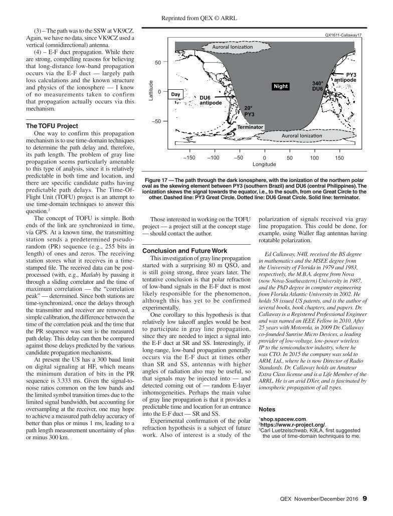
(5) – Predicts the “NE at SS, NW at SR” experience of low-band operators in the southern hemisphere. Take, for example, a link between southern Brazil and central Philippines (Figure 17). In this case, the ionization at or near the northern auroral oval refracts the signal from Brazil in the required direction — south, towards the equator, and onto a Great Circle leading to the Philippines. The antipode of the Brazilian station is near Okinawa, so it can employ gray line propagation for DX south of that point.
Assumptions Made in this HypothesisWhile the above may be persuasive,
the polar refraction hypothesis is based on several unproven assumptions.
(1) – Auroral oval ionization is as described, and does close the E-F duct and refract the incoming signal equator-ward. While the existence of the auroral oval is established fact, its function in refracting signals in the E-F duct has not been demonstrated.
(2) – The path was to the SSE, not SSW, at N4BRF. We have no data, since N4BRF used a vertical (omnidirectional) antenna.
50
0
–50
Latti
tude
–150 –100 –50 0 50 100 150Longitude
QX1611-Callaway15
30°N4BRF
335°VK9CZ
Day
Auroral Ionization
Auroral Ionization
Terminator
N4BRFantipode
VK9CZ antipode Night
QX1611-Callaway16
VK9CZ
N4BRFantipode
Figure 15 — The path to the north is not open because the skew required to move from one Great Circle to the other is to the north, but the ionization of the northern polar oval refracts
the signal towards the equator, i.e., to the south. Dashed line: N4BRF Great Circle. Dotted line: VK9CZ Great Circle. Solid line: terminator.
Figure 16 — Antipodes. For stations in North America, nearly all DX in Asia and Oceania is north of their antipode. This accident of geography drives the “SW at SR, SE
at SS” experience. [peakbagger.com/pbgeog/worldrev.aspx]
Figure 17 — The path through the dark ionosphere, with the ionization of the northern polar oval as the skewing element between PY3 (southern Brazil) and DU6 (central Philippines). The ionization skews the signal towards the equator, i.e., to the south, from one Great Circle to the
other. Dashed line: PY3 Great Circle. Dotted line: DU6 Great Circle. Solid line: terminator.
(3) – The path was to the SSW at VK9CZ. Again, we have no data, since VK9CZ used a vertical (omnidirectional) antenna.
(4) – E-F duct propagation. While there are strong, compelling reasons for believing that long-distance low-band propagation occurs via the E-F duct — largely path loss calculations and the known structure and physics of the ionosphere — I know of no measurements taken to confirm that propagation actually occurs via this mechanism.
The TOFU ProjectOne way to confirm this propagation
mechanism is to use time-domain techniques to determine the path delay and, therefore, its path length. The problem of gray line propagation seems particularly amenable to this type of analysis, since it is relatively predictable in both time and location, and there are specific candidate paths having predictable path delays. The Time-Of-Flight Unit (TOFU) project is an attempt to use time-domain techniques to answer this question.3
The concept of TOFU is simple. Both ends of the link are synchronized in time, via GPS. At a known time, the transmitting station sends a predetermined pseudo-random (PR) sequence (e.g., 255 bits in length) of ones and zeros. The receiving station stores what it receives in a time-stamped file. The received data can be post-processed (with, e.g., Matlab) by passing it through a sliding correlator and the time of maximum correlation — the “correlation peak” — determined. Since both stations are time-synchronized, once the delays through the transmitter and receiver are removed, a simple calibration, the difference between the time of the correlation peak and the time that the PR sequence was sent is the measured path delay. This delay can then be compared against those delays predicted by the various candidate propagation mechanisms.
At present the US has a 300 baud limit on digital signaling at HF, which means the minimum duration of bits in the PR sequence is 3.333 ms. Given the signal-to-noise ratios common on the low bands and the limited symbol transition times due to the limited signal bandwidth, but accounting for oversampling at the receiver, one may hope to achieve a measured path delay accuracy of better than plus or minus 1 ms, leading to a path length measurement uncertainty of plus or minus 300 km.
50
0
–50
Latti
tude
–150 –100 –50 0 50 100 150Longitude
QX1611-Callaway17
20°PY3
340°DU6
Day
Auroral Ionization
Auroral Ionization
Terminator
PY3antipode
DU6 antipode
Night
Those interested in working on the TOFU project — a project still at the concept stage — should contact the author.
Conclusion and Future WorkThis investigation of gray line propagation
started with a surprising 80 m QSO, and is still going strong, three years later. The tentative conclusion is that polar refraction of low-band signals in the E-F duct is most likely responsible for the phenomenon, although this has yet to be confirmed experimentally.
One corollary to this hypothesis is that relatively low takeoff angles would be best to participate in gray line propagation, since they are needed to inject a signal into the E-F duct at SR and SS. Interestingly, if long-range, low-band propagation generally occurs via the E-F duct at times other than SR and SS, antennas with higher angles of radiation also may be useful, so that signals may be injected into — and detected coming out of — random E-layer inhomogeneities. Perhaps the main value of gray line propagation is that it provides a predictable time and location for an entrance into the E-F duct — SR and SS.
Experimental confirmation of the polar refraction hypothesis is a subject of future work. Also of interest is a study of the
polarization of signals received via gray line propagation. This could be done, for example, using Waller flag antennas having rotatable polarization.
Ed Callaway, N4II, received the BS degree in mathematics and the MSEE degree from the University of Florida in 1979 and 1983, respectively, the M.B.A. degree from Nova (now Nova-Southeastern) University in 1987, and the PhD degree in computer engineering from Florida Atlantic University in 2002. He holds 58 issued US patents, and is the author of several books, book chapters, and papers. Dr. Callaway is a Registered Professional Engineer and was named an IEEE Fellow in 2010. After 25 years with Motorola, in 2009 Dr. Callaway co-founded Sunrise Micro Devices, a leading provider of low-voltage, low-power wireless IP to the semiconductor industry, where he was CTO. In 2015 the company was sold to ARM, Ltd., where he is now Director of Radio Standards. Dr. Callaway holds an Amateur Extra Class license and is a Life Member of the ARRL. He is an avid DXer, and is fascinated by ionospheric propagation of all types.
Notes1shop.spacew.com.2https://www.r-project.org/.3Carl Luetzelschwab, K9LA, first suggested