1 Status box Agenda item : 2d Title: GUIDANCE ON CHEMICAL MONITORING OF SEDIMENT AND BIOTA UNDER THE WATER FRAMEWORK DIRECTIVE Version no : 6 Date : 13 May 2010 Leaders of the Activity: France (Ineris), Italy (ISS/Min Env and CNR-IRSA), EC JRC Circulation and received comments: The mandate of the Chemical Monitoring Activity-1 on Monitoring Best Practices, including the preparation of the guidance on sediment and biota was agreed by the Water Directors at their meeting in November 2006. The first draft (version 4) of this guidance was presented and discussed at the March meeting of the Working Group E as well as the open issues. Comments have been requested in writing and based on them a new version has been produced filling some last gaps and taking all comments of MS into account. Version 5 was prepared for the Strategic Co-ordination Group meeting on 5-6 May. Final comments made at the Strategic Co-ordination Group meeting were incorporated into version 6. Disclaimer: This technical document has been developed through a collaborative programme involving the European Commission, all the Member States, the Accession Countries, Norway and other stakeholders and Non-Governmental Organisations. The document should be regarded as presenting an informal consensus position on best practice agreed by all partners. However, the document does not necessarily represent the official, formal position of any of the partners.
Transcript
1
Status box
Agenda item: 2d Title: GUIDANCE ON CHEMICAL MONITORING OF SEDIMENT
AND BIOTA UNDER THE WATER FRAMEWORK DIRECTIVE
Version no: 6 Date: 13 May 2010
Leaders of the Activity: France (Ineris), Italy (ISS/Min Env and CNR-IRSA), EC JRC
Circulation and received comments:The mandate of the Chemical Monitoring Activity-1 on Monitoring Best Practices, including the preparation of the guidance on sediment and biota was agreed by the Water Directors at their meeting in November 2006. The first draft (version 4) of this guidance was presented and discussed at the March meeting of the Working Group E as well as the open issues. Comments have been requested in writing and based on them a new version has been produced filling some last gaps and taking all comments of MS into account. Version 5 was prepared for the Strategic Co-ordination Group meeting on 5-6 May. Final comments made at the Strategic Co-ordination Group meeting were incorporated into version 6.
The Water Directors are invited to: discuss and endorse the final version 6 during the meeting in Spain on 27-
28 May 2010, so that a final edited version can be made publicly available.
Contact:Valeria Dulio (France/Ineris), Mario Carere (Italy/ISS), Georg Hanke (EC,JRC), Stefano Polesello (Italy/CNR-IRSA), Madalina David (EC,DG ENV), Caterina Sollazzo (Italy/Ministry of the Environment)
Disclaimer:This technical document has been developed through a collaborative programme involving the European Commission, all the Member States, the Accession Countries, Norway and other stakeholders and Non-Governmental Organisations. The document should be regarded as presenting an informal consensus position on best practice agreed by all partners. However, the document does not necessarily represent the official, formal position of any of the partners. Hence, the views expressed in the document do not necessarily represent the views of the European Commission.
COMMON IMPLEMENTATION STRATEGY FOR THE WATER FRAMEWORK DIRECTIVE
GUIDANCE ON CHEMICAL MONITORING OF SEDIMENT AND BIOTA
UNDER THE WATER FRAMEWORK DIRECTIVE
VERSION 6
MAY 2010
2
1. Scope of the guidance............................................................................................................51.1. Legal background-Sediment and biota chemical monitoring under the Water Framework Directive..........................................................................................................................................................5
1.2. Aim and structure of the guidance....................................................................................................6
1.3. Guidance documents for chemical monitoring................................................................................7
2. Terms and definitions.............................................................................................................7
3. Compound and matrix selection for sediment and biota monitoring.................................103.1. Introduction......................................................................................................................................10
3.2. Physico-chemical properties of chemical pollutants.....................................................................11
3.3. Selection of compounds to be monitored in sediment...................................................................11
3.4. Selection of compounds to be monitored in biota..........................................................................123.4.1. Organic compounds.....................................................................................................................123.4.2. Metals..........................................................................................................................................12
3.5. Criteria for matrix selection............................................................................................................12
4. Sampling strategy: general requirements and common aspects of sediment and biota monitoring.....................................................................................................................................15
4.2. Data analysis.....................................................................................................................................194.2.1. Method used for trend analysis of time series.............................................................................19
5. Monitoring of chemical substances in sediment.................................................................225.1. Sampling strategy for chemical monitoring in sediment..............................................................22
5.1.1. Selection of sediment sampling stations.....................................................................................225.1.2. Number of replicate samples per station.....................................................................................225.1.3. Sediment sampling frequency.....................................................................................................225.1.4. Sediment sampling depth............................................................................................................225.1.5. Sediment fraction to be analysed................................................................................................22
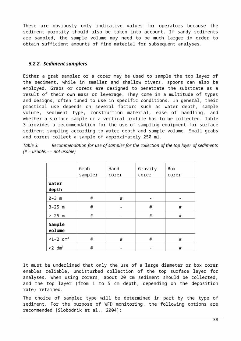
5.2. Technical aspects of sediment sampling.........................................................................................225.2.1. Sample volume............................................................................................................................225.2.2. Sediment samplers.......................................................................................................................225.2.3. Grab samplers..............................................................................................................................225.2.4. Corers..........................................................................................................................................225.2.5. Collecting of SPM and freshly deposited sediments...................................................................225.2.6. Transport and sieving..................................................................................................................225.2.7. Preservation & Storage................................................................................................................22
6.2. Sampling strategy for chemical monitoring in biota.....................................................................226.2.1. Selection of biota species and link with EQS derivation............................................................226.2.2. Recommendations for the selection of biota species..................................................................226.2.3. Selection of sites: general considerations....................................................................................226.2.4. Sampling period..........................................................................................................................226.2.5. Sampling frequency.....................................................................................................................226.2.6. Trend Analysis............................................................................................................................22
6.4. Choice of tissue for analyses and tissue preparation.....................................................................226.4.1. Fish..............................................................................................................................................226.4.2. Shellfish.......................................................................................................................................226.4.3. Pooling of specimens of biota.....................................................................................................22
7.1.1. Application in sediment monitoring............................................................................................227.1.2. Application in biomonitoring......................................................................................................22
7.2. Sediment ecotoxicity test for the evaluation of the ecological status and investigative monitoring....................................................................................................................................................22
8. Case studies..........................................................................................................................228.1. Case study 1.......................................................................................................................................22
8.2. Case study 2.......................................................................................................................................22
8.3. Case study 3.......................................................................................................................................22
8.4. Case study 4.......................................................................................................................................22
8.5. Case study 5.......................................................................................................................................22
8.6. Case study 6.......................................................................................................................................22
1.1.Legal background-Sediment and biota chemical monitoring under the Water Framework Directive
Directive 2008/105/EC (Environmental Quality Standards Directive) defines the good chemical status to be achieved by all Member States in 2015 and gives, together with the Water Framework Directive 2000/60/EC (WFD), the legal basis for the monitoring of priority substances in sediment and biota.
For the majority of the substances of the list of priority substances (33) and 8 certain other pollutants included in the Directive, the establishment of Environmental Quality Standards (EQS) at Community level has been limited to concentrations in the water column. However, as regards hexachlorobenzene, hexachlorobutadiene and mercury, it was considered impossible to ensure protection against indirect effects and secondary poisoning at Community level by EQS for surface water alone. It is therefore appropriate for these three substances to establish EQS for biota at Community level. In order to allow Member States flexibility depending on their monitoring strategy, Member States should be able either to monitor and apply EQS for biota, or to establish stricter EQS for surface water providing the same level of protection.
Furthermore, Member States should have the possibility to establish EQS (for the existing 33 priority substances + 8 certain other pollutants) for sediment and/or biota at national level and apply those EQS instead of the EQS for water set out in the Directive. Such EQS should be established through a transparent procedure, involving notifications to the Commission and other Member States, so as to ensure a level of protection equivalent to the EQS for water established at Community level. Moreover, sediment and biota remain important matrices for the monitoring of certain substances with significant potential for accumulation. In order to assess long-term impacts of anthropogenic activity and trends, Member States should take measures, subject to Article 3(3) of the EQS Directive, with the aim of ensuring that existing levels of contamination in biota and sediment will not significantly increase.
Article 3 of Directive 2008/105/EC:
“Member States may opt to apply EQS for sediment and/or biota instead of those laid down in Part A of Annex I in certain categories of surface water. Member States that apply this option shall:
a) apply, for mercury and its compounds, an EQS of 20 μg/kg, and/or for hexachlorobenzene, an EQS of 10 μg/kg, and/or for hexachlorobutadiene, an EQS of 55 μg/kg, these EQS being for prey tissue (wet weight), choosing the most appropriate indicator from among fish, molluscs, crustaceans and other biota;
b) establish and apply EQS other than those mentioned in point (a) for sediment and/or biota for specified substances. These EQS shall offer at least the same level of protection as the EQS for water set out in Part A of Annex I;
c) determine, for the substances mentioned in points (a) and (b), the frequency of monitoring in biota and/or sediment. However, monitoring shall take place at least once every year, unless technical knowledge and expert judgment justify another interval; and
d) notify the Commission and other Member States, through the Committee referred to in Article 21 of Directive 2000/60/EC, of the substances for which EQS have been established in accordance with point (b), the reasons and basis for using this approach, the alternative EQS established, including the data and the methodology by which alternative EQS were derived, the categories of surface water to which they would apply, and the frequency of monitoring planned, together with the justification for that frequency.
3. Member States shall arrange for the long-term trend analysis of concentrations of those priority substances listed in Part A of Annex I that tend to accumulate in sediment and/or biota, giving
5
particular consideration to substances numbers 2, 5, 6, 7, 12, 15, 16, 17, 18, 20, 21, 26, 28 and 30, on the basis of monitoring of water status carried out in accordance with Article 8 of Directive 2000/60/EC. They shall take measures aimed at ensuring, subject to Article 4 of Directive 2000/60/EC that such concentrations do not significantly increase in sediment and/or relevant biota.
Member States shall determine the frequency of monitoring in sediment and/or biota so as to provide sufficient data for a reliable long-term trend analysis. As a guideline, monitoring should take place every three years, unless technical knowledge and expert judgment justify another interval”.
Furthermore, monitoring of sediment and biota can also be used to describe the general contaminant status, and supply reference values for local and regional monitoring. Analyses of sediment and/or biota can be a cost-effective approach for initial screening of areas for contamination, to compare contaminant concentrations in different areas and to identify possible sources of contaminants. In using sediment and biota as a first level screening for certain chemicals in the monitoring programme, water measurements may be downscaled. The initial screening will help to identify areas of concern and areas where additional effort is needed, such as increased intensity of sediment, biota, or water monitoring or direct measurements.
1.2.Aim and structure of the guidance
This guidance document addresses the different requirements for compliance checking and temporal trend monitoring for biota and sediment, taking into account the obligations of the EQS Directive. The recommendations included in the guidance take into account current scientific knowledge and they should allow a harmonised implementation of sediment and biota monitoring across Europe.
The recommendations given in this guidance are addressed to surveillance, operational and investigative monitoring and should be applied to the current list of Priority Substances (33) + 8 other pollutants, but also to specific river basin pollutants which tend to accumulate in sediment or biota.
Chapter 3 gives recommendations for the matrix selection for the monitoring of chemical pollutants in different water bodies
There are some general parts of the monitoring strategy that are similar to sediment and biota, for example the application of the QA/QC Directive (Commission Directive 2009/90/EC); these issues are addressed in Chapter 4 of the guidance.
For compliance checking against EQS values, harmonisation of the different tools of monitoring programmes is needed: e.g. site selection, sampling strategy, selection of species (for biota), choice of analytical methods. These aspects are described in chapter 5 for sediment and in chapter 6 for biota.
Chapters 4, 5 and 6 contain also general recommendations:
- to assess compliance with the no deterioration objective of the WFD;
- to assess long-term changes in natural conditions and to the assess the long term changes resulting from widespread anthropogenic activities;
The assessment of the long-term impacts of anthropogenic activities includes the determination of the extent and rate of changes in concentrations of environmental contaminants.
In Chapter 7 are described complementary methods for monitoring.
The guidance has been harmonised with the technical guidance document on EQS derivation (TDG-EQS) that is in course of publication [EC, 2010].
The WFD also covers the protection of transitional, coastal marine and territorial waters for chemical status; thus, this guidance includes specific recommendations on these type of water categories..
6
1.3.Guidance documents for chemical monitoring
The Common Implementation Strategy of the Water Framework Directive comprises the development of guidance documents in relation to the implementation of this directive. The guidance documents have been created as request of Member States for further documentation of technical details important for harmonised implementation of environmental monitoring. The aim of these types of documents is to give further detail and thus facilitate the implementation of the WFD in the Member States, while also enhancing the degree of harmonisation, taking into account best available techniques, standard procedures and common practices.
Relevant for the purpose of the present guidance document is Guidance document No. 19 [EC, 2009] prepared by the Chemical Monitoring Activity Expert Group. Guidance document No.19 provides recommendations on the strategy for matrix selection and analytical aspects for analysis of water, sediments and biota under the WFD.
Thus both guidance documents are closely related and should be consulted together.
Another useful document will be the TGD-EQS in course of publication [EC, 2010] in which there is described the methodology for the derivation of EQS in water, sediment and biota.
Moreover, it is worth mentioning CIS Guidance document No. 7 [EC, 2003], which contains general aspects of monitoring requirements under the WFD and CIS Guidance document No. 15 [EC, 2007] which provides specific recommendations for groundwater monitoring.
Other useful guidelines relevant in the field of sediment and biota monitoring have been published in the context of OSPAR, HELCOM, MedPol Conventions and SedNet (see the reference).
2. Terms and definitions
Selected terms and definitions of specific importance for the chemical monitoring according to WFD are listed here. All other terms, which have already been agreed upon and defined elsewhere in WFD and associated documents, are not listed here, but are used without amendment.
Look out!
The guidance for chemical sediment and biota monitoring will have to be adapted to regional and local circumstances.
Look in:CIRCA public document library – guidance documents
Analysis of covariance: (ANCOVA) is a general linear model with one continuous outcome variable (quantitative) and one or more factor variables (qualitative). ANCOVA is a merger of ANOVA and regression for continuous variables. ANCOVA tests whether certain factors have an effect on the outcome variable after removing the variance for which quantitative predictors (covariates) account. The inclusion of covariates can increase statistical power because it accounts for some of the variability.
Analysis of variance: (ANOVA) is a collection of statistical models, and their associated procedures, in which the observed variance is partitioned into components due to different explanatory variables. In its simplest form ANOVA gives a statistical test of whether the means of several groups are all equal, and therefore generalizes Student's two-sample t-test to more than two groups. ANOVAs are helpful because they possess a certain advantage over a two-sample t-test. Doing multiple two-sample t-tests would result in a largely increased chance of committing a type I error. For this reason, ANOVAs are useful in comparing three or more means.
Bioconcentration Factor: See EQS guidance 2010
Bioaccumulation Factor: See EQS guidance 2010
Certified reference material: (CRM) reference material characterized by a metrologically valid procedure for one or more specified properties, accompanied by a certificate that provides the value of the specified property, its associated uncertainty, and a statement of metrological traceability.[ISO Guide 35:2006]
Composite sample: two or more samples or subsamples mixed together in appropriate proportions, from which the average result of a designed characteristic may be derived from the same stratum or at the same sediment thickness. The sample components are taken and pre-treated with the same equipment and under the same conditions.
Two or more increments or sub-samples mixed together in appropriate proportions, either discretely or continuously (blended composite sample), from which the average value of a desired characteristic may be obtained
[ISO 5667-12:1995 Water quality – Sampling - Part 12 Guidance on sampling of bottom sediments ISO 11074 2:1998]
Environmental specimen banking: ESB may be defined as the storage, under appropriate conditions, of material from which information about the state of the environment may be obtained afterwards.
Grab sample: samples taken of a homogeneous material, usually water, in a single vessel. Filling a clean bottle with river water is a very common example. Grab samples provide a good snap-shot view of the quality of the sampled environment at the point of sampling and at the time of sampling. Without additional monitoring, the results cannot be extrapolated to other times or to other parts of the river, lake or ground-water.
Lentic: refers to standing or still water. It is derived from the Latin lentus, which means sluggish. Lentic ecosystems can be compared with lotic ecosystems, which involve flowing terrestrial waters such as rivers and streams. Together, these two fields form the more general study area of freshwater or aquatic ecology.
Limit of detection: (LOD) means the output signal or concentration value above which it can be affirmed, with a stated level of confidence that a sample is different from a blank sample containing no determinand of interest.
8
[Commission Directive 2009/90/EC]
Limit of quantification: (LOQ) means a stated multiple of the limit of detection at a concentration of the determinand that can reasonably be determined with an acceptable level of accuracy and precision. The limit of quantification can be calculated using an appropriate standard or sample, and may be obtained from the lowest calibration point on the calibration curve, excluding the blank.[Commission Directive 2009/90/EC]
Lotic: refers to flowing water, from the Latin lotus, past participle of lavere, to wash. Lotic ecosystems can be contrasted with lentic ecosystems, which involve relatively still terrestrial waters such as lakes and ponds. Together, these two fields form the more general study area of freshwater or aquatic ecology.
Octanol-water partition coefficient: (kow) indicates hydrophobicity of a chemical substance
Quality: all the features and characteristics of a measurement result that bear on its ability to satisfy given requirements of quality[EN 14996:2006]
Quality assurance: all those planned and systematic actions necessary to provide adequate confidence that a product will satisfy given requirements of qualityNOTE This include AQC, audit, training, documentation of methods, calibration schedule, etc.[EN 14996:2006]
Quality control: operational techniques and activities that are used to fulfill requirements for quality.[EN 14996:2006]
Random sampling: form of sampling whereby the chances of obtaining different concentration values of a determinand are precisely those defined by the probability distribution of the determinand in question[ISO 5667- 6:2005 Water quality-Sampling- Part 6 Guidance on sampling of rivers and streams]
Reference material: (RM) material, sufficiently homogeneous and stable with respect to one or more specified properties, which has been established to be fit for its intended use in a measurement process.[ISO Guide 35:2006]
Sample: a limited quantity of something which is intended to be similar to and represent a larger amount of that thing(s).
Sampling frequency: Sampling frequency defines the number of samples per second (or per other unit) taken from a continuous signal to make a discrete signal.
Sampling point: precise position within a sampling site from which samples are taken[ISO 5667- 6:2005 Water quality-Sampling- Part 6 Guidance on sampling of rivers and streams. Modified definition]
Sampling station: a well delimitated area, where sampling operations take place[IUPAC 2005 Pure and Applied Chemistry 77, 827–841]
Sampling strategy: The result of the selection of the sampling points within a sampling site[IUPAC 2005 Pure and Applied Chemistry 77, 827–841]
9
Soil adsorption coefficient: (koc) Soil adsorption coefficient normalised by soil organic carbon content. Usually measured for environmental chemicals according to the OECD Test guideline 106
Statistical sampling: sampling whereby the samples are taken at predetermined interval (in space or time)[ISO 5667- 6:2005 Water quality-Sampling- Part 6 Guidance on sampling of rivers and streams. Modified definition]
Test portion: The amount or volume of the test sample taken for analysis, usually of known weight or volume.
Uncertainty of measurement: a non-negative parameter characterizing the dispersion of the quantity values being attributed to a measurand, based on the information used.[Directive 90/2009/EC]
Uncertainty arising from sampling: The part of the total measurement uncertainty attributable to sampling[EURACHEM/CITAC:2007 Measurement uncertainty arising from sampling: A guide to methods and approaches]
List of abbreviations
HELCOM The Baltic Marine Protection Commission also called Helsinki Commission
OSPAR The Convention for the Protection of the Marine Environment of the North-East Atlantic or OSPAR Convention
MEDPOL
The Med Pol Programme (the marine pollution assessment and control component of MAP) is responsible for the follow up work related to the implementation of the LBS Protocol, the Protocol for the Protection of the Mediterranean Sea against Pollution from Land-Based Sources and Activities (1980, as amended in 1996), and of the dumping and Hazardous Wastes Protocols.
3. Compound and matrix selection for sediment and biota monitoring
3.1. Introduction
The WFD classification of the chemical status of a water body is based on compliance with EQS. Directive 2008/105/CE sets the environmental quality standards for 41 substances in water matrix, but also gives an option to the Member States to derive EQS for sediment and/or biota. The frequency of monitoring of priority substances in the water column (whole water or dissolved) differs from those in sediment and biota and it is clear that the choice of the matrix to be monitored will be strategic in terms of costs and resources for compliance checking. The minimal frequency required for water monitoring of priority substances is once per month (once every 3 months for river-basin-specific pollutants), but for sediment and biota the monitoring frequency can be once per year unless technical knowledge and expert judgement justify another interval.
10
The main aim of the WFD is the achievement of good chemical status for all water bodies. However, Member States can decide the matrix for certain substances.
For instance, sediment represents a recommended matrix for the assessment of chemical status for some metals and hydrophobic compounds in marine and lentic water bodies. However in dynamic lotic water bodies, sediments do not often provide an appropriate matrix for compliance checking because of high variability. Furthermore, in such water bodies, sediments can either be too perturbed to be representative or in some cases absent. In these cases this assessment could be made by measurement of the concentrations in suspended solid matter (SPM). In large lowland rivers, freshly deposited sediment collected by sedimentation traps can be used instead of SPM. In the latter case the equivalence between SPM and freshly deposited sediment must be verified.
For the purpose of trend monitoring, for many substances sediment, or alternatively SPM, and biota are the most suitable matrices because they integrate, in time and space, the pollution in a specific water body; the changes of pollution in these compartments are not as fast as in the water column and long-term comparisons can be performed. Directive 2008/105/EC gives an indication of the substances that should be taken into consideration for trend monitoring as well as for the frequency of monitoring of those substances.
3.2.Physico-chemical properties of chemical pollutants
The choice of the matrix to be monitored depends firstly on the physico-chemical properties of the substances. The priority list of the WFD contains several (classes of) substances which have a low solubility in water, a corresponding high octanol/water partition coefficient (log KOW; see Table 1) and a high potential for bioaccumulation and bioconcentration.
3.3.Selection of compounds to be monitored in sedimentThe prime criterion for the selection of organic compounds to be monitored in sediments is their physico-chemical preference for the solid phase, i.e. a poorly soluble character in water. The more hydrophobic (water repulsing) a compound is, the less soluble it is in water, and therefore more likely to adsorb to sediment particles. A simple measure of the hydrophobicity of an organic compound is the octanol–water partition coefficient (Kow), which is a good predictor of the partitioning potential of the contaminant in the organic fraction of the sediment (Koc).
As a rule of thumb, compounds with a log Kow>5 should preferably be measured in sediments, or in suspended particulate matter (SPM), while compounds with a log Kow<3 should preferably be measured in water. For instance, HCB (hexachlorobenzene; log KOW=5.7) should not be preferably monitored in water, but in sediment or in suspended particulate matter, because of its preference to adsorb to sediment particles (i.e. organic carbon).
Look in:Directive 2008/105/EC
Art 3, paragraph 3: Member States shall arrange for the longterm trend analysis of concentrations of those priority substances listed in Part A of Annex I that tend to accumulate in sediment and/or biota, giving particular consideration to substances numbers 2, 5, 6, 7, 12, 15, 16, 17, 18, 20, 21, 26, 28 and 30, on the basis of monitoring of water status carried out in accordance with Article 8 of Directive 2000/60/EC. They shall take measures aimed at ensuring, subject to Article 4 of Directive 2000/60/EC, that such concentrations do not significantly increase in sediment and/or relevant biota.
11
Atrazine, on the other hand, with a log KOW~2.5, should be monitored in water and not in sediment, due to its high water solubility.
For compounds with a log Kow between 3 and 5, the sediment matrix or suspended particulate matter is optional and will depend on the degree of contamination. If the degree of contamination for a hydrophobic compound is unknown or expected to be low, sediment should be an additional monitoring matrix (due to accumulation).
3.4. Selection of compounds to be monitored in biotaThe prime criterion for the selection of compounds to be monitored in biota is their physico-chemical preference for this matrix (e.g. various metals and lipophilic compounds); the metabolisation and depuration efficiency of the different species should also be taken into consideration for biota monitoring (see Chapter 6).
According to the monitoring programmes and plenty of scientific studies, the most common substances analysed in marine biota are organochlorinated compounds (especially PCBs, DDT and its metabolites and organochlorinated pesticides), PAHs (only in mussels because they are partially metabolised in fishes), TBT, and trace metals that tend to accumulate.
3.4.1. Organic compoundsFor organic substances, monitoring in biota should be performed when biomagnification factor (BMF) is >1 or when bioconcentration factor (BCF) is >100; if no valid measured BMF or BCF (BAF) is available, a log Kow>3 can be considered as an indicator for bioaccumulation potential. The BMF is the ratio of the concentration of a substance in an organism compared to the concentration in food (prey) items. The BCF is the ratio of the concentration of a substance in an organism to the concentration in water.
It should also be ensured that there is no mitigating property such as rapid degradation (ready biodegradability or hydrolysis half-life <12h at pH 5-9, 20°C). If this is the case, then biota monitoring is not recommended. Information on molecular size can be an indicator of limited bioaccumulation potential of a substance, as very bulky molecules will pass less easily through cell membranes.
3.4.2. MetalsBiomagnification of metals in aquatic organisms is rarely observed and, if it does occur, it usually involves the organo-metallic forms of metals (e.g. methylmercury); a lack of biomagnification should not be interpreted as lack of exposure or no concern for trophic transfer. Even in the absence of biomagnification, aquatic organisms can bioaccumulate relatively large amounts of metals and this can become a significant source of dietary metal to their predators.
For metals, a BCF should not be used; this is because the model of hydrophobic partitioning, giving a more or less constant ratio Cbiota/Cwater with varying external concentration, does not apply to metals. Further indications for metals are included in the TGD-EQS [EC, 2010].
3.5. Criteria for matrix selectionBased on the rule of thumb mentioned above, a distinction has been made between preferred (P), optional (O) and not recommended (N) matrices for the monitoring of priority substances in Table 1.
- Preferred (P): Monitoring should be performed in this matrix.
- Optional (O): Monitoring can be performed in this matrix, but also in other compartments/matrices; the choice will also be made on the basis of the degree of contamination of a particular matrix.
- Not recommended (N): Monitoring in this matrix is not recommended unless there is evidence or the possibility of accumulation of the compound in this matrix.
12
For metals, because of the high variability of these compounds, this distinction cannot be made except when they are in the form of organometals (e.g. methylmercury).
In some cases, sediment and biota are both preferred matrices and the choice should be made on the basis of local contamination and on the basis of the EQS derived.
These criteria are not mandatory and Member States can choose the appropriate matrix on the basis of their knowledge, nevertheless keeping in mind the indications of Directive 2008/105/EC.
13
Table 1Monitoring matrices for the priority substances and certain other pollutants listed by the EQS Directive. The substances in red are those suggested by Directive 2008/105/EC for sediment and biota trend monitoring. The values of the log KOW are taken from the Chemical Monitoring Guidance n.19. The values of BCF are taken from the datasheets of the priority substances in the public section of the CIRCA forum(http://circa.europa.eu/Members/irc/env/wfd/library?l=/framework_directive/i-priority_substances/supporting_background/substance_sheets&vm=detailed&sb=Title).
P = preferred matrix, O = optional matrix., N = not recommended, n.a. = not applicable
Priority Substance BCF Log KOW Water Sediment / BiotaAlachlor 50 3.0 P O N_Anthracene 162-1440 4.5 O O OAtrazine 7,7-12 2.5 P N NBenzene 13 2.1 P N NBrominated diphenyl ethers a 14350-1363000 6.6 N P PCadmium and its compounds n.a. n.a. n.a. n.a.C10-13-chloroalkanes 1173-40900 4.4-8.7 N P PChlorfenvinphos 27-460 3.8 O O OChlorpyrifos (-ethyl, -methyl) 1374 4.9 O O O1,2-Dichloroethane 2-<10 1.5 P N NDichloromethane 6,4-40 1.3 P N NDi(2-ethylhexyl)phthalate (DEHP) 737-2700 7.5 N O ODiuron 2 2.7 P N NEndosulfan 10-11583 3.8 O O OFluoranthene 1700-10000 5.2 N P PHexachlorobenzene 2040-230000 5.7 N P PHexachlorobutadiene 1,4-29000 4.9 O O PHexachlorocyclohexane b 220-1300 3.7-4.1 O O PIsoproturon 2,6-3,6 2.5 P N NLead and its compounds n.a. n.a. n.a. n.a.Mercury and compounds c n.a. N O P Naphthalene 2,3-1158 3.3 O O ONickel n.a. n.a. n.a. n.a.Nonylphenols d 1280-3000 5.5 P P OOctylphenol d 471-6000 5.3 P P OPentachlorobenzene 1100-260000 5.2 N P OPentachlorophenol 34-3820 5.0 O O OPolyaromatic Hydrocarbons e 9-22000 5.8-6.7 N P P Simazine 1 2.2 P N NTributyltin compounds 500-52000 3.1-4.1 O O P
Trichlorobenzenes 120-3200 4.0-4.5 O O OTrichloromethane 1,4-13 2.0 P N NTrifluralin 2360-5674 5.3 N P ODDT (including DDE, DDD) 6.0-6.9 N P PAldrin 6.0 N P PEndrin 5.6 N P PIsodrin 6.7 N P PDieldrin 6.2 N P PTetrachloroethylene 3.4 O O NTetrachloromethane 2.8 P N NTrichloroethylene 2.4 P N Na Including Bis(pentabromophenyl)ether, octabromo derivate and pentabromo derivateb HCH (all isomers) - BCF (lindane)c methylmercuryd Nonyl- and Octylphenols do not follow the classical Kow partition, because they can establish hydrogen bonds by the phenolic hydroxyl.eIncluding Benzo(a)pyrene, Benzo(b)fluoroanthene, Benzo(g,h,i)perylene, Benzo(k)fluoroanthene, Indeno(1,2,3-cd)-pyrene. For these compounds the metabolisation in higher trophic levels should be taken into account.
4. Sampling strategy: general requirements and common aspects of sediment and biota monitoring
The main purpose of any measurement is to enable decisions to be made. Fitness for purpose is therefore the most important requirement of any sampling strategy. The fitness for purpose of a sampling design, however, can only be judged from reliable estimates of its uncertainty and its impact on the monitoring objectives. Current practice in the estimation of uncertainty in environmental monitoring follows the general principles set out in the “Guide to Expression of Uncertainty in Measurement” [ISO 1993] whose underlying philosophy has been endorsed in all standardisation documents issued by International and National Standardisation bodies. The notion of “uncertainty” is closely related to other concepts of measurements such as “accuracy”, “error”, trueness, bias and precision [EURACHEM, 1995]. In this context the following important differences are to be recalled [EURACHEM, 2007]:
- Uncertainty is a range of values attributable on the basis of a measurement result and other known effects, whereas “error” is a single difference between a result and “true value”.
- Uncertainty includes allowances for all effects that may influence results (i.e. both random and systematic errors); precision only includes the effects that vary during the observations (i.e. only some random errors).
- Uncertainty is valid for correct application of measurement and sampling procedures, but it is not intended to make allowances for gross operator errors.
It becomes therefore apparent that the act of taking a sample introduces uncertainty into a measurement result. In addition, sampling protocols are never perfect, as they cannot anticipate the possible eventuality in the moment of sampling.
In the context of this guidance, the main sources of uncertainty related to sediment and biota monitoring are the natural spatial and temporal variability within the sampling site (or population) as well as the measurement process including the act of sampling, sub-sequent steps of sample pre-treatment and storage until the actual measurement. Natural variability and the act of sampling itself are certainly the most important contributors and least controllable.
While sampling and measurement can be assessed to a certain degree using classical tools for quality control and measurements such as field blanks, reference materials, intercomparisons and so forth, the influence of the natural variability can only been dealt with if sufficient information on the system is available in the planning phase of a monitoring programme. The higher the complexity or heterogeneity of the studied water body, the higher the number of samples to be investigated and hence the more expensive the monitoring becomes.
In this context the proper definition of the scope and objectives of the monitoring programme are of pivotal importance, because they are crucial factors to define the sampling site, frequency, duration and the methodology, including sample pre-treatment and subsequent measurements and tests. A leitmotif is that the monitoring should be designed in such a way that possible errors occurring during sampling and measurement can be statistically detected.
A preliminary or exploratory sampling programme can be useful to provide relevant information for designing the final sampling programme. In exploratory studies, data may be statistically analysed in several ways for several purposes. However there should still be a clear understanding of what must be measured from what population and how the samples are to be selected. The sampling strategy is an intrinsic component of the data, and may limit their use and interpretation. Quantitative objectives for a selected primary purpose should therefore also be established for exploratory studies.
15
4.1.Statistical considerations
CIS WFD Guidance Documents No. 7 [EC, 2003] and No. 19 [EC, 2009] give already some general indications with regard to underlying statistical principles. It is not simple to decide frequency, number and time periods of sampling during the planning of the monitoring program without the aforementioned preliminary/exploratory campaign. However, it is clear that in the course of a monitoring programme further adaptation may be necessary.
Although sediment and biota are somewhat buffered towards fast changes in water quality, they are subject to random or systematic/seasonal variations. This needs to be considered, too. The derived statistical parameters such as the mean value, standard deviation, highest observed value or percentiles can only be estimates of the “true value”, which usually deviates from these data. In the case of randomly distributes values, which follow a normal or log-normal distribution, estimates become more reliable with an increased number of repetitions.
In case of systematic (e.g. cyclic) variations of the system under investigation, the choice of the sampling time is crucial in order to either capture the entire cycle or to cover maximum and minimum values.
4.1.1. Quantitative objectivesAs mentioned above, a proper definition of the monitoring objectives is vital. For a correct estimate of frequency, length of time series, density of sampling grid, etc., a quantification of the objectives is necessary. In this context one may distinguish between two types of monitoring studies, which however are frequently overlapping in reality:
- temporal monitoring studies, aiming at the detection of temporal trends in the investigated matrix. Since sediment and biota are generally buffered in their reaction time to chemical stress (if compared the water column), longer time series in general covering several years are needed to detect significant changes;
- spatial monitoring studies, aiming at the identification of spatial distribution pattern and anomalies. For sediment and biota monitoring being less subject to short-term variability, normal distribution may be assumed.
The ISO Standard 5667-1:2006 [ISO, 2006] gives appropriate indications on how to determine the necessary number of samples for the various purposes of monitoring. Some recommendations from this standard set are worth mentioning here:
- while random variations follow usually a normal or log-normal distribution, systematic variations are either following trends or cyclic patterns or a combination of both;
- the predominant type of variation (random vs. systematic) may vary for the same matrix for different compounds;
- if random variations are predominant (see preliminary investigations), the moment of sampling is less important;
- if cyclic variations are predominant a systematic and regular sampling pattern is to be preferred;
- in case of doubt, random stratified sampling is the best compromise. In any case statistical considerations should be at the basis of decisions concerning the number of samples to be taken.
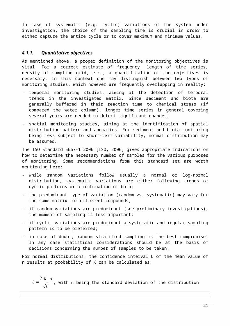
For normal distributions, the confidence interval L of the mean value of n results at probability of K can be calculated as:
, with being the standard deviation of the distribution
16
Example: With a confidence interval of 10% around the mean value, a confidence level of 95% and a standard deviation of 10%, the number of samples to be taken is calculated as:
, hence n = 61 Samples. This is translated for instance into the sampling of 1 to 2
samples per week, if the monitoring period is equal to one year.
The careful definition and description of the objectives of the monitoring study includes:
- the choice of the sampling matrices with a strict definition of the sampling units and a description of what they represent in time and space (this description is a prerequisite for an appropriate interpretation of the results);
- the definition of the required sensitivity of the programme, i.e. the smallest change to be detected for temporal studies or smallest difference between areas for geographical studies;
- the definition of the statistical power to detect such a difference at a specified significance level.
The definition of the sensitivity and statistical power of the programme are essential in order to properly estimate, for example, the number of samples per sampling occasion, length of the time-series, sampling frequency etc., required for the investigation. This power will decrease as sources of variance (analytical variance, natural environmental variance) increase.
On the consequence, in order to calculate, for example, the number of samples and the sampling frequency required to fulfil those objectives, an estimate of the sample variance is needed. Expected variance estimates could, perhaps, be extracted from similar ongoing monitoring programmes or, what is more reliable, be assessed from a pilot project using the same sampling strategy, sampling matrices etc., as the currently planned monitoring programme.
The necessary or possible power of a monitoring programme will vary with the purpose of the investigation and with the contaminant, matrix and area being investigated. It is thus not possible to give fixed values for all situations. It is the duty of the programme manager to specify the size of the changes the monitoring programme is expected to identify and at what power, or for the programme executor to estimate what it is possible to achieve. It is however essential that the quantitative objectives are determined before any monitoring programme is started.
A quantified objective for temporal studies could, for example, be stated as follows:
- To detect a 50 % decrease within a time period of 10 years with a statistical power of 80 % at a significance level of 5 %. (A 50 % decrease within a time period of 10 years corresponds to an annual decrease of about 7 %).
And for spatial studies, for example as follows:
- To detect differences of a factor 2 between sites with a power of 80 % at a significance level of 5 %.
A significance level of 5% means that we are prepared to accept a risk of 5% to conclude from our data that there is a trend or difference when there actually is not. Similarly, a power of 80% means that we accept a risk of 20% to conclude that there is no trend or difference when it really is one. Statistical power and methods to estimate power are discussed in detail in Cohen [1988].
In the case of temporal monitoring studies, when no trend is found, it is essential to know whether this indicates a stable situation or that the sampling strategy is too poor to detect even major changes in the contaminant load to the environment. One approach for solving this problem would be to estimate the power of the time series based on the ‘random’ between-year variation. Alternatively the lowest detectable trend could be estimated at a fixed power to represent the sensitiveness of the time series. It should be stressed that the power estimate must be interpreted with great caution. A matrix showing a very high power is not necessarily a good matrix for monitoring. If the matrix analysed does not respond to the environmental changes being monitored, the between-year variation would probably be low and consequently the power high. Another problem is that a single outlier could ruin an estimate of the between-year variation.
17
Bearing these difficulties in mind, and as an example for the purpose of trend monitoring, the quantified objective could be stated as follows:
- to detect an annual change of 5% within a time period of 10 years with a power of 90% at a significance level () of 5% with a one-sided test.
It has to be stressed though, that statistically significant trends do not guarantee that detected temporal trends are a result of a causal relation between concentration and time. If the samples are biased, not comparable over time or if relevant confounding co-variants are not accounted for, “false-trends” may occur.
The statistical assessment of trends always also requires experts whose experience allows them to undertake a more accurate evaluation of the analysis results.
4.1.2. Representativity
4.1.2.1. The sample matrix
A first important aspect is the representativity of the sampling matrix in relation to the contaminant load and exposure in the studied monitoring site. It is therefore essential that the suggested sampling matrices are thoroughly described concerning what they represent in relation to contaminant load or exposure. In addition to factors like availability, sampling costs etc., additional information on, for example, concentration factors, bioaccumulation rates, metabolic capacity and excretion rates, for biota, would be useful. Various tissues within the same species vary considerably with respect to the above-mentioned factors i.e. they may represent totally different ranges of time and space. They may also react to changes in the environment very differently.
Similar considerations are needed when considering the use of sediment as a monitoring matrix. The concentrations of both organic and inorganic contaminants in sediment are very dependent upon the bulk properties (e.g. particle size distribution, and organic carbon content) of the sediment. Concentrations are much higher in fine grained sediment than in the sand or coarser fractions. A spatial survey of contaminant concentrations in sediment is often very strongly influenced by the spatial distribution of muddy sediment. Normalisation techniques have been developed to minimise the influence of differences in bulk composition between sediment samples and to reduce the potential for “false trends” in temporal data series arising from changes in bulk composition unrelated to contaminant inputs. The application of normalisation techniques needs to be planned as part of the preparation of samples prior to analysis, or to ensure that the appropriate determinands for normalisation are included in the suite of analytes.
4.1.2.2. Spatial representativity
A second aspect to be considered is the representativity of the sample in relation to the spatial variability of the sampling site. Questions such as: “How many sampling sites do we need in order to appropriately represent a region?” will inevitably be raised when monitoring contaminants. Any firm advice from a statistical point of view needs estimates on spatial heterogeneity. For spatial studies the objectives have to be clearly specified (e.g. spatial trends, differences between regions etc) and made quantitative.
A variogram may be used to describe the spatial correlation structure [Cressie, 1993; Davis, 1986]. Normalisation processes to reduce between-sample variance should be applied to field data before such a variogram is constructed, particularly for analyses of sediment.
In practice, such variograms are not available or may not be available for all monitoring areas, and some pragmatic approach, based on prior experience may be necessary. This emphasises the need for preliminary monitoring revealing useful information.
18
4.2.Data analysis
Data must be expressed as mean values and standard deviation, reporting also the number of analysed samples (n) and the range of measured values. This information should be completed by additional information which may be relevant in the context of the monitoring (percentiles, trend analyses, etc.)
In any case data analysis should be performed in a transparent way with appropriate statistical methods to reveal and compare status and trends at local, regional, national, European scales.
Differences between periods and or sites can be tested by one- or two-way analysis of variance (ANOVA) or by multivariate methods such as cluster analyses (CA), principal component analyses (PCA) or positive matrix factorisation (PMF). Multiple Pearson correlations can reveal significant relationship between chemicals and co-linearity of regressions can be tested by covariance analyses (ANCOVA). Chemical concentrations trends can also be assessed by correlating their variations with time and Spearman’s rank correlation used to assess their predictable co-variance; the Spearman’s rank correlation statistical test has been widely applied to evaluate individual contaminants at site, regional and national scales.
4.2.1. Method used for trend analysis of time series
The main goal of trend analysis is to test objectively whether there is a meaningful systematic change in the time series, assessed against some measure of the random noise in the observations. The output from this component will usually be the probability that the test statistic of the used method could have arisen by chance when there is no trend. If this is less than some pre-specified value (e.g. 5 %), the result is considered to be significant, that is: the null hypothesis of no trend is rejected. What constitutes a meaningful change will depend on the objectives of the assessment, and is a major consideration in the choice of method as discussed in section 4.1.1.
For the trend assessment the following four separate but complementary components are identified:
1. graphical presentation of the time series with a summary line to indicate the general trend; presenting time series grouped by region, by substances, or by originating country., could provide a further opportunity to identify common trends, or common data anomalies, e.g., a consistent extreme value in a given year.
2. a formal test of trend, with trend defined in an appropriate way for the context of the assessment;
3. a quantification of the tendency to increase or decrease;
4. a power analysis which reflects the detectability of a possible trend.
The statistical method used to assess trends should be:
robust, i.e., to be both routinely applicable to many data sets, and to be as insensitive as possible to statistical assumptions (e.g. Normal distribution) and problematic numerical features such as extreme data values, partial bulking of samples, and values less than LOD;
intuitive, i.e., for the results of the analysis to be understandable without a detailed understanding of statistical theory;
revealing i.e. to provide easy access to several layers of information about the major features of the data-both those of direct interest such as evidence of simple trends, and the more negative features, such as missing years, years with all results below the limit of detection, extreme values, and so
In the context of trend assessment the method should be sensitive to the kinds of changes of concern in the assessment. Not all tests are equally effective at detecting all patterns of change. For a very focused test, this may be a disadvantage if all patterns of change are of interest, or an
19
advantage if this focus is on patterns of interest. Three groupings of patterns of change may be considered to be of interest:
1. linear trend
2. monotonic non linear trends,
3. non-monotonic trends.
Hence, if the purpose of the assessment is to detect monotonic trends and has to be robust in the sense that it is unaffected by isolated extreme values, the Mann-Kendall test would be appropriate. If the purpose is to detect all trends, then the choice is between the compound Mann-Kendall test and the smoothers, with a final decision depending on the weight given to the other factors.
The statistical procedures currently used by OSPAR for trend detection in Northern seas are described in the “CEMP Assessment Manual for contaminants in sediment and biota”. [OSPAR, 2008]. The method used by OSPAR involves the use of a weighted smoother, and assessment for significant linear and non-linear trends. Fitting a weighted smoother is straightforward if the statistical weights are known beforehand. The statistical weights should be inversely related to the total environmental and analytical variance each year. Appropriate methods for estimating them will depend on the QA information available.
The weighting is a function of the performance of the laboratories in annual external Quality Assurance schemes (Laboratory Performance Studies). In the absence of external QA performance data, that the data points are all given equal weight.
For a mixture of theoretical and practical reasons, OSPAR Commission found appropriate to adopt three different approaches to data analysis, based upon the length of the available time series:
3-4 years compute the average of the median log-concentrations.
5-6 years fit a linear regression to the median log-concentrations and test the significance of the linear trend.
>6 years fit a smoother to the median log-concentrations and test its significance, followed by tests of the significance of the components of linear and non-linear trend.
Although a linear regression model could have been fitted to data for 3 or 4 years, the power of this test would be low. Further, where significant trends did occur, they would be more likely to reflect short-term trends than long-term changes. For these reasons, a simple summary of the average level was thought to be more useful. Similarly, it seems inappropriate to attempt to describe non-linear trends in time series with fewer than 6 years.
Essentially, for each dataset with data for 6 or more years, the method is to summarise trends using a smoother; a non-parametric curve fitted to median log-concentrations. This summary is supported by a formal statistical test of the significance of the fitted smoother, and by tests of the linear and non-linear components of the trend.
Few statistical assumptions are required for the fitted smoother to be valid. Mainly, the annual contaminant indices should be independent with a constant level of variability. For the statistical tests to be valid, there is a further assumption that the residuals from the fitted model should be lognormally distributed. The theory and methodology are described in detail in Nicholson et al. [1998].
20
4.3.Quality Assurance/Quality Control
The quality and comparability of analytical results generated by laboratories appointed by competent authorities of the Member States to perform sediment and biota chemical monitoring pursuant to Article 8 of Directive 2000/60/EC should be ensured.The Commission Directive 2009/90/EC represents the legal basis for the performance of the analytical methods and gives technical specifications for chemical monitoring. Based on the requirements of this directive, the application of internal and external quality control measures, such as the use of blanks, standards, (certified) reference materials or the regular participation in laboratory inter-comparison, is strongly recommended.
Look in:Commission Directive 2009/90/EC
Article 1 Subject matterThis Directive lays down technical specifications for chemical analysis and monitoring of water status in accordance with Article 8(3) of Directive 2000/60/EC. It establishes minimum performance criteria for methods of analysis to be applied by Member States when monitoring water status, sediment and biota, as well as rules for demonstrating the quality of analytical results.
Article 3 Methods of analysis Member States shall ensure that all methods of analysis, including laboratory, field and on-line methods, used for the purposes of chemical monitoring programmes carried out under Directive 2000/60/EC are validated and documented in accordance with EN ISO/IEC-17025 standard or other equivalent standards accepted at international level.
Article 4 Minimum performance criteria for methods of analysis 1. Member States shall ensure that the minimum performance criteria for all methods of analysis applied are based on an uncertainty of measurement of 50 % or below (k = 2) estimated at the level of relevant environmental quality standards and a limit of quantification equal or below a value of 30 % of the relevant environmental quality standards.
21
5. Monitoring of chemical substances in sediment
5.1. Sampling strategy for chemical monitoring in sediment
General criteria and good practices for sediment sampling strategy are already reported in CIS Guidance Document No. 19 [EC, 2009].
Sampling strategies for sediment monitoring may have two major approaches: a probabilistic design, where sampling points are randomly selected within the sampling site, and a targeted design, where sampling points are selected based on the analysis of pressures and pre-existing knowledge of point sources.
Probabilistic design is more appropriate for diffuse source characterisation, whereas targeted design is better suited for the implementation of the WFD at surveillance, operational and investigative monitoring sites.
In targeted designs, sampling points are selected based on prior knowledge of other factors such as water depth, bottom topography, nature of the sediment (clay, sand, pebbles, peaty), contaminant loading and accessibility.
In general, targeted sampling is appropriate for situations in which:
- the site boundaries are well defined;
- the objective of the investigation is to screen an area for the presence or absence of contamination. In CIS Guidance No. 19 [EC, 2009], section 4.3, it is further stated that "...areas can be cost-efficiently scanned using sediments and biota to compare contaminant levels in different areas and to identify possible sources of contaminants to the area". And "In using sediments and biota as a first level screening for certain chemicals in the monitoring programme, water measurements may be downscaled. The initial screening will help to identify areas of concern and where to direct effort, such as follow up with water samples and direct measurements.";
- information is desired for a particular condition (e.g., “worst case”) or site;
- schedule or budget limitations preclude the possibility of implementing a statistical design.
For trend analyses, the sampling strategies and the procedures of examination and analyses of sediments should ensure that continuity with pre-existing monitoring programmes is maintained. Any changes should only be made if comparability with long-term data is guaranteed. This also includes continuing to use suspended particulate matter (SPM) or freshly deposited sediments collected by sediment traps or sedimentation boxes as an alternative to sediments for monitoring contaminants in large lowland rivers.
5.1.1. Selection of sediment sampling stations
General criteria for the selection of monitoring sites in WFD monitoring programmes are discussed in CIS Guidance documents No. 7 [EC, 2003] and No. 19 [EC, 2009].
Whatever the water body, sediments should be sampled at sites that are representative of the water body or cluster of water bodies. This requires understanding of the hydrological and geo-morphological characteristics and the pollution sources. This information can be derived from earlier studies, current monitoring programmes or a preliminary dedicated survey.
Sediments are much less temporally variable, but inherently much more heterogeneous than waters. The homogeneity of a sampling area may be checked in a pilot phase by defining one or more transects (according to the area extent), where five sampling points for each transect are selected. In each sampling point, five or more independent surface sediment samples have to be
22
collected. An aliquot for each sample should be analysed after homogenisation and sieving (see Section 5.2.6). The homogeneity can be checked for the between-sample (between sampling points in the transect) and the within-sample (within sampling points) variance, using an Anova/F-test. If the within-sample variance is of the same order as, or even exceeds, the between-sample variance, the whole transect should be considered as a single sampling site.
The areas where homogeneity has thus been checked will serve for the identification of the sampling sites and the number of replicates. Owing to the physical heterogeneity of the sediment, statistical analyses should be carried out on data normalised with respect to the fine fraction (see 5.1.5).
There is no need for even distribution of sampling sites in a water body. In a homogeneous water body, such as a pristine lake, the number of sampling sites may be relatively low. But if gradients are to be expected as a result of changing morphological and/or input conditions, or of areas that are of concern (‘hot spots’), a higher number of sampling sites should be defined.
Known point sources, e.g. from present or past industries, need special attention, as they are not representative and may bias the overall evaluation of a given water body. Tributaries often have different water and thus also different suspended matter/sediment characteristics from the receiving river or lake. Receptor water bodies should be sampled downstream the discharges or the tributary confluence, at a point where complete mixing has been established. According to Art. 4 of Directive 2008/105/EC, mixing zones should be designated by Member States. The Technical Guidance document for the identification of mixing zones under Article 4(4) of the EQS Directive is currently under development.
Net deposition areas with soft sediments characterised by relatively high amount of fine fraction (the fraction <63 mm, consisting of silt and clay) are preferred as sampling sites, whereas areas where sediments contain peat, pebbles or rocks, compacted sediments, or coarse sand should be discouraged. As a rule of thumb, sediments should contain at least 5% fine fraction (<63 µm), information which may have to be obtained from preliminary trial surveys.
Alternatively, especially in the cases of rivers without sediments or with perturbed sediments, SPM and freshly deposited sediment can be used to collect the desired fine fraction. Knowing that deposition of suspended particles from the water column is favoured in areas with relatively low energy in the water (waves, currents), the following general criteria can be provided for the selection of the sampling sites:
- in rivers and transitional waters (estuaries), the currents are highest in the central channel or river bed, and as a consequence this results in a relatively low amount of fines deposited on the bottom. Higher concentrations of fine-grained deposits are found in areas where the water flow is lower, such as near the side of the river (in concave stretches of the river) and in accumulation areas within estuaries;
- in natural estuaries with complex suspended solids dynamics (i.e. estuaries with settling and erosion zones, tidal flats, etc.), representative sampling is possible only upstream of the tidal limit. In such cases, the sampling site should be located in the non-tidal zone of unidirectional flow (e.g. upstream of a weir);
- in lakes and reservoirs the highest energy dissipation occurs near the inlet of rivers, and on the shores (wave action). The highest concentration of fines may therefore be found away from these sites;
- in coastal waters, areas with high tidal currents shall be avoided. Sedimentation areas, such as embayments or areas of relatively deep water, are preferred.
When the final objective is the assessment of a temporal trend in chemicals contamination, a representative number of sites should be selected, giving preference to sites used for surveillance monitoring. The same sampling sites should be used over the years. This requires continued accessibility, and also that the sampling site, and the related sampling points, are well defined by exact geographic coordinates, stating also the datum of the reference system. Finally, the site should be large enough to supply multiple samplings if sediment cores are taken.
23
5.1.2. Number of replicate samples per station
Multiple samples have to be collected at each sampling site in order to estimate factors contributing to the overall variance in the analytical data. It is recommended that three to five samples (independent replicates) are selected at each site.
QA/QC procedures should also cover the sampling phase, as it is part of the overall measurement process. The sampling procedures adopted in routine monitoring of sediments quality should be validated and sampling quality control performed. Validation allows the evaluation of the sampling quality under stated (routine) conditions and provides an estimation of the contribution of sampling to the measurement uncertainty (including the analysis). It can be performed by taking replicate (duplicate) samples (6–10 in the pilot phase) at a same point, differing as little as possible one from the other in terms of space and time. In general, only the random component of uncertainty (repeatability) arising from sampling may be assessed. Replicating the analyses on each duplicate, the contribution due to the analytical phase is also evaluated. Pooling of individual samples into one composite sample is not recommended in the pilot phase as this prevents the estimation of field variability, which is an essential parameter for power analysis and trend tests.
Since the potential range of substances to be analysed is wide, the sampling quality performances may be reasonably assessed only for a selected measurand (e.g. metals).
Whatever the sampling quality requirements, the sampling procedure performance may be kept under control during routine sampling activity by applying the same, previously validated, sampling procedure at the same sampling point. Quality control may be performed through the collection of replicate samples, as in the validation, and setting up a quality control chart. Frequency of sampling quality control depends on the extent of the sampling locations and of the planned sampling frequency.
5.1.3. Sediment sampling frequency
As a result of a usually limited sedimentation rate (usually in the range 1–10 mm/y, but larger values occur) and the physical and biological mixing of surface sediments, the composition of sediments generally is usually rather stable in comparison to the concentrations of contaminants in the water column, except for rivers characterised by turbulent flow. As a consequence, sampling of sediments generally requires i a lower frequency than e.g. sampling of surface waters.
Directive 2008/105/EC states that monitoring should be performed at a minimum frequency of once every year for compliance with EQS, while for temporal trend analysis once every three years, unless technical knowledge and expert judgement justify another interval.
Sediment samples should be collected at an appropriate frequency that matches the expected changes in the sediment, taking into account the hydrological regime and the sedimentation rate of the water body studied. Estuaries, rivers and reservoirs, and sometimes lakes, may show large differences in hydrodynamic characteristics over the year. The higher the expected/observed changes, the higher the frequency.
In highly dynamic water bodies such as estuaries, sampling several times per year may be required. However, the application of normalisation techniques (see Sections 5.1.5 and 5.4, below) can greatly reduce the variability arising from changes in the bulk properties of sediment (e.g. changes in particle size distribution arising from changes in water flow regimes).
It is recommended that sampling be undertaken during a period with low current velocities, and the preferred period corresponds to the time of lowest water discharge rate (flow). Moreover, bioturbation is lowest in the winter period. It is recommended to plan the sampling campaigns in the same time window every year, preferably under similar flow conditions.
Special attention should be given to sites significantly affected by changing sediment input, in which water flow and therefore accumulation rates may change seasonally, following, for example, flood events or ice cover. Sampling during or shortly after a flood should be avoided.
24
If high fluctuation in the concentration of contaminants during the year is measured or expected at selected hot spots, higher frequencies should be adopted.
It might be helpful to distinguish between variations in physics (e.g. high and low run-off periods) which lead to changes in bulk sediment composition (% sand, % mud etc.) and thereby lead to changes in the concentrations of contaminants when looking at the whole sediment, and processes such as seasonality in use of herbicides that lead to changes in pollutants load in sediment. The former should be addressed through normalisation methods, while the latter should be addressed by increasing sampling frequency.
Sediment sampling frequency could be reduced when parameters are demonstrated, by monitoring data and the analysis of pressures, to be significantly below the quality targets or when no significant trend can be observed or expected.
When monitoring for temporal trends, sound statistical analysis will require several data points in time. Notwithstanding that the WFD reporting cycle is six years, a recommended approach might be to sample annually for the first WFD cycle in order to allow a trend analysis with better statistical confidence for that cycle, and then reduce the frequency thereafter if considered appropriate. Trend analyses after 12 or 18 years would continue to make use of the assessed data from the first six years.
Sampling of suspended solids for trend analysis should be carried out at least 4 times a year, although monthly sampling should be the goal. The median of a year should be used to observe the trend, as it is less sensitive to the outliers (this eliminates, for example, findings made at times of high water, which are less representative for trend observation).
5.1.4. Sediment sampling depth
Sediment monitoring generally addresses the top layer of the sediment because this layer indicates the actual deposited material and the actual status of pollution. Furthermore, the top layers of the sediment form the habitat of benthic organisms, and the protection of ecosystems is the main aim of WFD. These top layers are the net result of deposition of particulate matter from the water column (sedimentation) and physical (e.g. by currents, waves) and biological mixing (bioturbation), which is restricted in most areas to the top 5–10 cm. Sediments and SPM are sources of food and are subject to dynamic interactions with the water column due to resuspension.
The main criterion for choosing the correct sediment sampling depth (the thickness of the sediment layer sampled) in a water body is the knowledge of the deposition rate of the sampling site. In theory, the lower the deposition rate, the thinner the layer that one may want to sample. In situations with steady sedimentation and undisturbed sediments, such as some oligotrophic lakes, the very top layer of the sediment will contain the most recent information and thinner top layers may be sampled (from 0.5 to 1 cm depth).
In practice, apart from this kind of specialised environment where bioturbation and physical disturbance of sediment are negligible and undisturbed surface sediments can be sampled, it is recommended to sample the top layer of the sediment, from 1 to 5 cm depth, depending on the deposition rate. The sampling depth should be defined for each sampling site. In the case of highly perturbed sediment or in large fast flowing rivers, the sediment sampling depth could be more than 5 cm. For comparison reasons, sampling depths should be maintained over the years for the respective sites.
Different intervals may be appropriate for the sampling of sediment core profiles.
25
5.1.5. Sediment fraction to be analysed
Sediments consist of a large range of particles, ranging from the very fine clays (<2 mm) to coarse pebbles and stones of several mm in size. Their surface is often coated by organic matter, which acts as a binding site for many pollutants and other compounds. The smaller the particle, the larger the relative surface area, and the greater part of many hazardous substances is consequently contained in the finer sediment fractions, which are also the primary food source for biota.
Fine material (inorganic and organic) and associated contaminants are preferentially deposited in areas of low hydrodynamic energy, while in areas of higher energy, fine particulate matter is mixed with coarser sediment particles, which generally have a much smaller capacity to bind contaminants. This dilution effect arising from the presence of coarser material will cause lower and variable contaminant concentrations in the resulting whole sediment. Obviously, grain size is one of the most important factors controlling the distribution of natural and anthropogenic components in sediments, along with organic matter content. It is, therefore, essential to normalise for the effects of grain size in order to provide a basis for meaningful comparisons of the occurrence of substances in sediments of variable grain size distribution and texture within individual areas, among areas or over time.
When analysing whole sediment (i.e. <2 mm fraction) for spatial distribution surveys, the resulting maps may give a direct reflection of pollutant distribution only if the sediments have homogeneous bulk composition (e.g. are all mud, or are all sand) throughout the whole surveyed area. However, in areas with varying grain size distributions, a map of contaminant concentrations will be closely related to the distribution of fine-grained sediments, and any effects of other sources of contaminants, for example anthropogenic sources, will be at least partly obscured by grain size effects. If samples used for a spatial survey consist predominantly of fine material (>80% fines), the influence of grain size distribution is of minor importance and may be neglected avoiding the need for sieving procedures.
In temporal trend monitoring, too, differences in grain size distribution can obscure trends.
Selection of the grain size fraction considered as the ‘fine fraction’ used for the analysis depends on the general aim of the sediment analysis; it should reflect the distribution of the particular analyte as a function of the sediment particle size.
Sieving to collect fraction <20 µm is an effective way to reduce variability. In most areas, however, the portion of 20–63 µm is rather small compared to the fraction <20 µm. For pragmatic reasons (labour-intensive sieving process to collect very fine fractions) analysis of the grain-size fraction <63 µm, representing the clay-silt fraction, is widespread in many current monitoring programmes. Consequently the recommended procedure for the correction for grain size effects in sediments is the collection of the sediment fraction <63 µm. This recommendation is made recognising the effort required to undertake the sieving process and the added risk of contamination.
In some water bodies, such as estuaries of large mainland rivers, the 20–63 µm fraction is not negligible. In these cases, even when sieving at <63 µm, co-factors (see Section 5.4) still need to be determined.
An alternative procedure, based on the normalisation to the <63 µm fraction, can be recommended in order to avoid the sieving process and the associated risk of contamination. As concentrations of contaminants in sandy sediments are usually negligible, chemical substances (both organic and inorganic compounds) may be analysed in the <2 mm fraction and subsequently normalised to a sample consisting of 100% of the <63 µm fraction. In order to get reliable normalised results, the amount of fines should be at least 10%. Moreover, with this alternative procedure it is mandatory to measure the actual granulometry of the analysed sediment sample.
SPM or freshly deposited sediment in rivers can be used as a source of material <63 µm, except in particular hydrological situations, such as floods, when large particles can be moved and redeposited.
26
5.2. Technical aspects of sediment sampling
The ISO 5667 series of standards provides guidance on sampling techniques; the followings should be taken into account for sediment sampling:
- Design of sampling programmes [ISO, 2006];
- Preservation and handling of samples [ISO, 2003];
- Sampling of rivers and streams [ISO, 2005];
- Sampling from lakes [ISO, 1987];
- Sampling of bottom sediments [ISO, 1995];
- Guidance on preservation and handling of sludge and sediment samples [ISO, 1999];
- Sampling of marine sediments [ISO, 2004].
Notwithstanding the importance of the general principle presented in the standards, which should be known by the staff carrying out the sampling, the exact procedure/equipment will always be dependent on the conditions at the actual sampling site. As sampling sites may be rather different, the staff should be sufficiently experienced to decide on the appropriate procedure/equipment. In general, the technical aspects of sampling do not depend on the water body concerned, but on the logistic requirements. Shallow waters may be present in any water body, deep waters are present in many lakes and coastal environments. The sampling operation is technically driven more by water depth than by the type of water body.
Even before sampling starts, it is important to check whether the sampling site is disturbed by unexpected events (tourism, boating, debris, etc). Samples should be collected from physically undisturbed sediments. For example, in manual sampling near the shoreline, the person taking the sample should avoid sampling in his footsteps.
It is good practice to complete a sampling report, which may include a general description of collected samples including colour, homogeneity (presence or absence of stratification), presence or absence of animals (indication of bioturbation), surface structures, odour and any visible contamination (e.g., oil sheen).
Furthermore, contamination during sampling, sample pre-treatment (sieving, homogenising, freeze drying) and storage of samples has to be avoided. Other sources of contaminant degradation (oxidation, photodegradation) should be minimised.
Many further manuals, which describe technical procedures for sediment sampling, are available [see e.g. U.S. EPA, 2001; Kramer et al., 1994; Mudroch and Azcue, 1995; UNEP/MAP, 2007].
5.2.1. Sample volume
Sample volume is dependent on:
- The (expected) concentration of the hazardous substances (for organic micro-pollutants the sample volume should be larger than for trace elements);
- The percentage of the fine fractions which accumulate contaminants;
- The number of analyses that need to be carried out on the sample (nutrients, trace metals, organic micro-pollutants, radio-tracers, co-factors, etc.);
- The number of replicates for each analysis.
Obviously, for surface sediment samples, replicates may provide a larger sample volume, but for vertical profiles the volume of slices of sediment will remain limited. Samples obtained by corer are usually rather limited in volume (for a top 5 cm sample, an 8 cm Ø corer gives a sample of about 250 ml). In general it is recommended to obtain the following sample volumes. (Table 2):
27
Table 2. Recommended sediment sample volumes
Type of analysis Volume
Trace elements 50 ml
Organic micro-pollutants 200 ml
These are obviously only indicative values for operators because the sediment porosity should also be taken into account. If sandy sediments are sampled, the sample volume may need to be much larger in order to obtain sufficient amounts of fine material for subsequent analyses.
5.2.2. Sediment samplers
Either a grab sampler or a corer may be used to sample the top layer of the sediment, while in smaller and shallow rivers, spoons can also be employed. Grabs or corers are designed to penetrate the substrate as a result of their own mass or leverage. They come in a multitude of types and designs, often tuned to use in specific conditions. In general, their practical use depends on several factors such as water depth, sample volume, sediment type, construction material, ease of handling, and whether a surface sample or a vertical profile has to be collected. Table 3 provides a recommendation for the use of sampling equipment for surface sediment sampling according to water depth and sample volume. Small grabs and corers collect a sample of approximately 250 ml.
Table 3. Recommendation for use of sampler for the collection of the top layer of sediments (# = usable; - = not usable)
Grab sampler
Hand corer
Gravitycorer
Box corer
Water depth0–3 m # # - -
3–25 m # - # #
> 25 m # - # #
Sample volume<1–2 dm3 # # # #
>2 dm3 # - - #
It must be underlined that only the use of a large diameter or box corer enables reliable, undisturbed collection of the top surface layer for analyses. When using corers, about 20 cm sediment should be collected, and the top layer (from 1 to 5 cm depth, depending on the deposition rate) retained.
The choice of sampler type will be determined in part by the type of sediment. For the purpose of WFD monitoring, the following options are recommended [Slobodnik et al., 2004]:
- sand: both grab and corer systems can be used;
- clay: it may be necessary to use a corer because a grab system may not penetrate easily into the clay;
28
- consolidated bottom sediment: both grab and corer systems can be used;
- unconsolidated (very soft) bottom sediment: grab systems are not suitable, as they are prone to sink through the top layer. Corer systems perform better.
Analyses of depth profiles can be used to get additional information on the history of contamination and to reconstruct the past trend. This approach is best applied in sediments where the sediment accumulation rate is high and the rate of disturbance (physical or bioturbation) is sufficiently low so as to cause negligible disturbance to the contaminant profiles. Sediment profile samples are collected exclusively by corers.
5.2.3. Grab samplers
Grab samplers are normally mounted on a winch and attached to a rope or pole. The limited weight of small grab samplers allows operation by hand, which could prove convenient in the field. The sampler is locked in the open position and lowered to some distance above the bottom sediment. It is important to reduce the lowering speed when approaching the bottom as a bow wave may flush away the fine sediment before the sampler reaches the bottom. When the sampler touches the surface sediment, a latch is released allowing the ‘jaws’ to close when the cable/pole is pulled up, thus collecting a surface sediment sample. The grab sampler should be retrieved slowly to ensure that the jaws dig into the sediment and to avoid loss of the surface layer.
After retrieval, the sampler is lowered into a clear tray. Before opening the jaws, the water contained above the sediment is gently siphoned away, taking care not to wash away fine sediments at the same time. After discarding the water, the grab sampler is opened and emptied in the tray.
Problems in sampler operation include their sinking too deeply into very soft sediments, mixing of the target surface sediment layer, not collecting sufficient sediment in hard substrates, or stones between the jaws preventing their closure.
To minimise contamination, sediment that has been in contact with the sampler is to be avoided, and surface samples are collected from the central part of the sample. Stainless steel versions minimise contamination of the sample (beware of contamination of Ni and Cr). Other materials for grab samplers include coated steel samplers, but they may contaminate samples for trace element analysis (rust, paint). Alternatives are aluminium samplers.
5.2.4. Corers
Core samplers are used when information concerning the vertical profile of the sediment is of interest, or when grab samplers cannot be used because of, for example, the sediment type.
Corer tubes are usually made of PVC or Perspex, the latter offering an immediate view of the sample collected. A polyethylene inner sleeve may be used to protect the sample from contamination by the corer wall. For the determination of trace organic pollutants, other materials such as stainless steel could be chosen to minimise contamination.
Hand-operated corers can conveniently be used to collect surface sediments: they may be a short plastic tube of 8 cm Ø and are manually pushed into the undisturbed sediment for about 30 cm. If necessary, the air on top is replaced by ambient water, a rubber stopper is inserted and the sampler is retrieved. A cap is placed immediately at the bottom end. Then the water is siphoned off, and the top 5 cm of sediment is collected; a piston may help to push out the sediment. A hand operated corer with an extension tube or rod can be used to water depths up to about 3 m, depending on the currents. The core length obtained is limited by the diameter of the tube and the friction of the tube wall: maximum core length @ (tube diameter)2. Hand corers have limited use for collecting profiles.
29
Gravity corers in principle act in a similar way to hand-operated corers, but in deeper water. The attached weight pushes the corer tube into the sediment. Often a valve is placed in the top section, preventing spillage of the sample during retrieval. Because of their weight, gravity corers are not easy to operate manually, and a winch is usually required. Core length is limited for the same reasons as for hand-operated corers, and they are of limited use for profile samples.
Box corers are very heavy, specialised equipment that collects large diameter undisturbed cores, from which replicate sub-samples may be collected (e.g. by hand-operated corer). As they are usually operated from research ships, they can be used in water depths >3 m. Usually the core length is maximum 1 m, and consequently they are of limited use for the collection of long profile samples. Operation requires specialised staff.
Usually one core is collected per sampling point. Within one core there is a chronology between different sediment layers. A replicate core, even collected nearby, may have a different sedimentation history and corresponding sediment depths may be different. Unless samples are collected by multi-corer, where the tubes are mounted in parallel and the distance between the cores is marginal, pooling of replicate samples is not recommended.
The distribution of sub-samples should be concentrated near the surface. The top of the sediment would be sliced to e.g. 3–6 slices (1–3 cm thick) and the lower part of the sample would be collected for reference.
5.2.5. Collecting of SPM and freshly deposited sediments
The following techniques are primarily used to collect suspended solid samples: centrifuge pumps and stationary or mobile settling basins or suitable traps/collection crates. In addition, samples of suspended solids can be collected through filtration. However, in the last case the sample quantity is generally small and therefore barely sufficient for an analysis, especially of the organic substances.
Sampling with centrifuge pumps usually takes several hours and has more the character of individual samples while settling basins generally collect monthly composite samples. In fact, sedimentation traps or boxes may be exposed to the water for two to four weeks, to sample suspended sediments carrying the present contaminants. This sampling technique has the advantage that samples represent the very last deposited layers, especially in slow-flowing continental mainland rivers, which can be also used for trend analysis.
Settling basins do not allow for quantitative separation of the suspended solids from the water phase, and fine grains in particular are not collected in full. In contrast, centrifuge pumps almost completely separate suspended solids from the water, but they could influence the particle size distributions. These characteristics should be taken into account when the sampling methodology is chosen.
5.2.6. Transport and sieving
All samples must be sieved over 2 mm mesh as soon as possible after collection to remove large detritus and benthic organisms. Otherwise, during subsequent sample handling and processing, such as storage, freezing or ultrasonic treatment, biotic material will deteriorate and become part of the sediment sample. In order to minimise the potential for disturbance of the sediment/water equilibrium wet sieving is best performed at the sampling point with ambient water. The same water should be reused to prevent changing equilibrium If field sieving is not possible, sieving should take place in the laboratory under controlled conditions.
Samples (sieved or not) are transferred preferably into wide-mouth, pre-cleaned bottles of amber glass (or aluminium, or other non-contaminating material) for organic analysis or into plastic bags or bottles for trace element analysis. Alternatively, amber glass jars can be used for all kinds of contaminants. Sampling containers should be filled to the top (minimal headspace) to reduce the
30
likelihood of oxidation and loss of acid volatiles sulphide (AVS) during transport. It is preferable to store samples under refrigeration (about 4°C) and transport them as soon as possible to the laboratory. Refrigeration is easily accomplished with cooling boxes and cooling inserts.
Transport of cores is critical as the integrity of the core has to be maintained. Samples near the sediment/water interface will be disturbed and will mix when transported in a horizontal position, thus losing their profile characteristics. In addition, even when transported in the vertical position, vibration will tend to compact the sediment. If possible, cores should be sub-sampled and sieved directly in the field.
Until the final sieving procedure that isolates the fines for subsequent analyses (see Section 5.1.5), which is normally carried out in the laboratory, the sample can be stored at 4°C for about a week and up to 3 months when frozen at -20°C, unless otherwise specified in the analytical methods for specific degradable compounds. Whenever possible, freezing should be avoided because it can change the grain size distribution of the sediment.
In the case of the AVS measurement, sediment should be preferably kept at 4°C, although freezing has negligible effects on AVS levels. If stored at 4°C, the period between sampling and AVS analysis should be no longer than two weeks.
If provided by the sampling strategy (see Section 5.1.5), the silt+clay fraction (<63 µm) could be separated by sieving over a 63 mm mesh sieve. As clays tend to form lumps of considerably larger diameter, sediments should be sieved wet. A minimum amount of ambient water should be used. It is strongly recommended to avoid sediments becoming dry. If it happens, sediments should be pre-soaked in water for at least 2 hours to break up the lumps.
In the case of saline samples it is particularly important to sieve with water with approximately the same salinity as at the sampling location. If no local water is available, the correct salinity value can be obtained by diluting a stock of seawater collected from the open sea.
Sieving may be carried out by simple means, using a sieve mounted on a funnel filled with water and moving the sieve manually. For the processing of larger numbers of samples, sieves may be placed on vibrator tables. The water can be efficiently separated from the sieved material by centrifugation. Sieving procedures have been described and evaluated in the QUASH project [QUASH, 1999; Smedes et al., 2000].
Sieves are traditionally made of corrosion-resistant brass (rim and mesh). Today, stainless steel is preferred for organics analyses. These must not be used for the analysis of trace metals, however. For trace metals, polymer sieves are recommended (PVC or acrylic rim, with e.g. nylon or polyester mesh).
5.2.7. Preservation & Storage
Storage begins when the samples are taken. All storage methods will affect the sample to some extent, and the choice of preservation technique depends mainly on the objective of the sample collection. Because the first few hours after sampling are the most critical for changes to occur in the sample, preservation steps should be taken, where possible, immediately upon sample collection. No recommendations can be given for a universal preservation or storage technique. A technique for one group of analyses may interfere with other analyses. To overcome this problem, a sufficient sample volume should be collected to allow specific preservation or storage techniques for each specific group of analytes.
Temperature is the most important factor affecting the samples, from the time of sample collection through handling to the final analyses. Another source of contamination is the adsorption of contaminants from laboratory air. Degradation and volatilisation of pollutants could be a source of errors too.
In the laboratory, the sieved sediment samples should be deep-frozen at -20°C and, when frozen, freeze-dried in a freeze-dryer as soon as possible. Check contamination during freeze-drying by placing a glass jar with 2 g C18 bounded silica in the freeze dryer in parallel with the samples.
31
Air-drying is not appropriate due to high contamination risks. Besides, samples may be difficult to disaggregate and mineral structures may be affected. If a freeze-dryer is not available, in order to limit microbial breakdown, the samples could be air- or oven-dried at 25 – 30°C till more or less constant weight as soon as possible after sieving. Losses of some determinands (volatile or semi-volatile compounds, such as e.g. 2–3 rings PAHs) can occur during this process, even when the drying is done at cool temperatures (<30°C). Prior to analyses of inorganic constituents (e.g. metals), sediment samples may be dried at 105°C (except for mercury determination, which needs a drying step at <50°C).
Containers for storing lyophilised or dried sediment samples are preferably wide-mouth bottles with a screw cap. Samples taken for the analysis of organic contaminants must be stored in amber glass, polytetrafluoroethylene (PTFE), stainless steel or alumimium containers. Sediments collected for analysis of metals can be stored in closed plastic or glass containers. Since sediment particles have a small surface area which exchanges with the container surface, the contamination risk is limited and it is possible to use a glass jar for all determinations in order to simplify sediment characterisation.
For mercury, samples must be stored in acid-washed borosilicate glass or quartz containers, as mercury can move through the walls of plastic containers. For organotins, storage of samples is preferably done in amber glass bottles, but containers of other materials such as polycarbonate or aluminium are also suitable. Maximum suggested time of storage of freeze dried sediment before analysis is about 180 days (30 days for Hg) if stored in a cool, dark place.
Archiving sediment samples is a must in QA/QC procedures. All samples should be kept for the duration of the monitoring in order to be able to come back to any of them, or to all of them, in case of problems in the analysis or interpretation. In addition, it may be useful to archive part of the original sample in order to be able to re-analyse the material for (other) compounds at a later date. Freeze-dried sediments remaining after analyses are stored in the original sample bottle, closed with an airtight lid to protect against moisture. When stored in a cool, dark place, samples may be archived and stored for 10-15 years, i.e. for the duration of the monitoring programme. For less stable compounds this period may be less.
5.3. Analytical methods
Only a few standard methods exist for sediment analysis (for PBDE, Cd, Pb, Ni, pentachlorophenol, tributyl tin compounds) [Lepom and Duffek, 2005]. As regards the soil analysis, the standard methods are missing for 10 substances only. However, existing ISO standard methods for soil analysis, summarised in CIS Guidance No. 19 “ANNEX I: List of ISO Standards for soil analysis” [EC, 2009], may be applied to sediments after validation on the appropriate matrix.
JAMP Guidelines for Monitoring Contaminants in Sediments [OSPAR, 2003] currently contain detailed advice on sampling, sample preparation and analytical methods for some contaminants in marine sediment. OSPAR Guidelines currently cover metals, chlorobiphenyls, PAHs, mono-, di- and tributyltin, PBDEs and HBCD; advices on PFOS, alkylated PAHs, co-planar CBs and dioxins in sediment are currently under development.
The analytical methods applied after extraction or digestion of the sediment, are generally the same for water and sediment samples. The principles of available analytical methods for priority substances are reviewed in CIS Guidance No. 19 “ANNEX II: Substance Guidance Sheets” [EC, 2009].
The use of standardised methods is recommended, because these methods have been finally validated in interlaboratory trials. Nevertheless, not all standardised methods meet the minimum performance criteria stated in the Directive 2009/90/EC. The use of standardised methods should only be mandatory if the analysis or the quantification contains “method-defined” parts. This is the case for e.g. the selection of congeners of brominated diphenyl ethers, the quantification of alkylphenols, and both the selection and quantification of short chain chlorinated paraffins, if available.
32
The methods will, to some degree, dictate the amount of sediment sample required for each analysis. Vice versa the amount of sample used in an analysis affects the detection limits attainable by a particular method.
5.3.1. Organic compounds
Solvent extraction methods described in standards for soil can also be used for dried sediment. EPA has adopted various extraction procedures, from classical Soxhlet extraction to advanced techniques such as Microwave Assisted Solvent Extraction (MASE) and Pressurised Solvent Extraction (PSE).
Special care should be taken for volatile compounds for which extraction of wet samples, avoiding the freeze-drying step, could be preferable. Extraction of wet sediment samples requires the use of a first extractant that is miscible with water (such as acetone), followed by a less polar extractant such as pentane or hexane. This procedure works well for non-polar priority substances such as organochlorinated pesticides, PAHs, PBDEs and chlorinated benzenes.
Alternative extraction methods for volatile compounds use purge-and-trap or headspace techniques.
The analytical techniques for semi-volatile organic compounds generally involve solvent extraction from the sediment matrix. Extensive cleanup is required if there is a likelihood of (a) biological macromolecules, (b) sulphur from reduced sediments and (c) oil and/or grease in the sediment.
The recommended detection method for analysis of semi-volatile and volatile organic pollutants in sediment is based on the use of capillary-column gas chromatography (GC) with mass spectrometry (MS). For the determination of organohalogenated compounds, GC with Electron Capture Detector (ECD) can be also used. The most selective methods using GC/MS techniques are recommended for most organic compounds, because such analysis can often reduce problems caused by matrix interferences.
Non-volatile organic compounds require HPLC separation with selective detection such as fluorescent and electrochemical detection. Standard methods based on mass spectrometric detection with atmospheric pressure ionisation hyphenated to liquid chromatography systems are under development.
5.3.2. Metals
For the determination of metal concentrations in sediment, samples must be digested with concentrated inorganic acids in a traditional open system or, more commonly, in sealed vessels in a microwave oven and analysed by methods such as inductively coupled plasma-atomic emission spectrometry (ICP-AES) or ICP-MS, graphite furnace atomic absorption spectroscopy (GFAAS) or atomic fluorescence spectrometry.
OSPAR recommends the inclusion of HF in the digesting medium [OSPAR, 2003]. By this approach, the total metal content, including that part of geochemical origin, is measured and that procedure allows the application of normalisation co-factors based on Al or Li content (see 5.4). This approach requires knowledge of the distribution of background concentrations of trace metals of geochemical origin.
In surface waters, background concentrations are less assessed and are very variable in a water body. HF digestion could lead to an overestimation of the trace metals content. The use of less aggressive acid mixtures (such as for example concentrated nitric acid + hydrochloric acid, Aqua regia), which are moreover safer substitutes, is therefore recommended, depending also on the final detection technique.
SEM-AVS (Simultaneously Extracted Metals – Acid Volatile Sulphides) analysis should be carried according to the United States Environmental Protection Agency (US-EPA) method [U.S. EPA,
33
1991] integrated by the Dutch National Institute for Public Health and the Environment (RIVM). Extraction with 6M HCl solution should be carried out on a homogenised wet sample. The formed H2S gas, collected in a NaOH-solution, is spectrophotometrically determined at 660 nm using dimethyl-p-phenylenediamine hydrochloride as colour reagent. Metals are determined on the filtered supernatans.
5.3.3. Quality Assurance / Quality Control procedures
Proper Quality Assurance/Quality Control procedures include the validation of methods by analytical laboratories, routine internal QC procedures and independent external QC procedures.
The validation of an analytical method, including the determination of measurement reliability, bias, etc., requires the use of certified reference materials. In CIS Guidance No. 19-“ANNEX III: Existing certified reference materials” [EC, 2009], a complete list of sediment certified reference materials (CRM) is reported. CRMs are currently available for the determination of metals, PAH and chlorinated pesticides in sediment. For other organic priority substances, no suitable CRMs have been developed yet.
Internal QC procedures should include the routine monitoring of the performance of analytical methods, for example by the inclusion of duplicate samples or (laboratory) reference materials in analytical batches. The results from these samples should be assessed using standard statistical methods such as Shewhart charts to ensure that the methods remain under statistical control.
It is recommended that laboratories participate in suitable external interlaboratory comparisons. A grouping of Proficiency Testing Laboratories has been established to meet the needs of WFD. This PT–WFD network (http://www.pt-wfd.eu/) is comprised of organisers of proficiency tests which support the implementation of the EU Water Framework Directive. It seeks to ensure that the demands of the EU WFD are met through the organisation of high-quality proficiency tests which are performed in a harmonised and comparable way.
5.4. Normalisation co-factors
Normalisation is defined here as a procedure to correct contaminant concentrations in sediment for the influence of the natural variability in bulk sediment composition (grain size, organic matter and mineralogy).
Isolation of the fine fraction by sieving can be regarded as a physical normalisation to reduce the differences in sediment granulometric composition (see Sections 5.1.5 and 5.2.6).
In data reporting, any geochemical-based differences in sediment composition that remains after sieving can be corrected for by the use of co-factors. It is also mandatory to report raw data, expressed as weight pollutant/weight sediment, together with normalising co-factors and/or normalised data.
For the analysis of trace elements in the sieved fine fraction, a common normalisation method involves the use of the aluminium (Al) concentration. Clay minerals are rich in (e.g.) Al or Li, the sands (quartz) are not. Generally, compared to aluminium, more accurate normalised data can be expected using lithium. Total sediments are analysed for the trace element, including the co-factor; the trace metal concentration is normalised with respect to the normaliser content that represents the fine fraction (normaliser content in sample minus the normaliser content in pure sand or in the >63µm fraction). In this case Al or Li is used as a proxy to fine sediment particles. The aluminium content in the sandy fraction may, however, vary from area to area. Therefore, to use this method, a statistically meaningful relationship between Al and grain size must be established in the sediment of the area prior to the application of the method.
For the analysis of trace organic compounds in sediment, a widely used normalisation method involves normalisation using the total organic carbon (TOC) concentration. Clay and silt minerals are coated with organic matter; while the coarser fractions contain relatively very small amounts of
TOC due to their small relative surface area. The ratio of [concentration of the organic compound]/[TOC] is the normalised value. However, care has to be taken, as organic matter in a sample is not always well defined and it can be composed of material with different properties. Furthermore, the nature of the organic matter may show spatial variation. Also, while normalisation using TOC is effective for lipophilic substances such as chlorinated compounds and PAHs, it may not be valid for other classes of compounds which bind to particles and clays with more polar bonds.
Detailed guidance on the use of normalising parameters for sediments is given in the Annex 5 of the JAMP Guideline for Monitoring Contaminants in Sediments [OSPAR, 2003; see also OSPAR, 2001].
35
6. Monitoring of chemical substances in aquatic biota
6.1. Introduction
The monitoring of chemical substances in aquatic biota should be performed according to the minimum requirements of Directive 2008/105/EC and according to the recommendations in CIS Guidance No. 19 [EC, 2009] and in the EQS Guidance document in course of publication [EC, 2010].
The objectives of biota monitoring under the WFD are:
- compliance checking against EQS values for the purpose of the classification of chemical (for the 33 priority substances and 8 certain other pollutants) and ecological status (in the case of river basin-specific pollutants) of the waterbodies.
- long-term trend analysis of concentrations of substances that tend to accumulate in biota in the context of surveillance monitoring programmes of WFD.
The substances to be monitored in aquatic biota should be selected on the basis of the recommendations given in Chapter 3.
The monitoring of mercury, hexachlorobenzene (HCB) and hexachlorobutadiene (HCBD), substances for which a European EQS has been derived, should be performed in accordance with the recommendations contained in this chapter.
Biota monitoring programmes under international conventions for inland, transitional, coastal and marine waters already exist: e.g. Helsinki Commission (HELCOM), OSPAR, International Commission for the Protection of the Rhine (ICPR), MEDPOL. In general, species that are already used in existing national or international monitoring programmes should be used for biota monitoring under Directive 2008/105/EC.
The methodology to determine the natural background concentrations of metals in biota is included in the EQS guidance in course of publication.
6.2.Sampling strategy for chemical monitoring in biota
The biota sampling strategy for a given water body should include the choice of the substances to be monitored (see Chapter 3), the selection of the species representative for that specific water body, the selection of the sampling sites, the monitoring frequency and the monitoring techniques.
The natural variability within biota samples should be reduced by an appropriate sampling design, keeping in mind that differences in age, size, sex and sexual maturity status can affect the measured concentrations of contaminants. Sampling strategies should be devised so as to minimise the impact of these factors. Biota sampling should only take place when fish and bivalves are in a stable physiological state, and outside the normal period of spawning. Fishes should be collected from areas characterised by relatively low natural variability.
Moreover, the following general recommendations are given:
- For the selection of species for biota monitoring, Member States should not use species that are endangered or that require special protection in compliance with “Habitat Directive” requirements or any other national or international action plan for nature conservation. Active biomonitoring, such as caging and transplantation procedures must avoid the introduction of allochthonous species to waterbodies. Non-native species should not be used in active biomonitoring.
- Sampling strategies for biota monitoring should seek for continuity with pre-existing monitoring programmes when relevant. In some cases and for some species, harmonisation with the biota sampling performed for the purpose of the classification of the ecological status can be useful.
36
6.2.1. Selection of biota species and link with EQS derivation
In the selection of biota species, consideration should be given to the main purposes of the EQS Directive: trend monitoring and compliance with EQS. Where possible, the same species sampled should be used for both purposes.
The species should be selected mainly on the basis of their ability to reflect the quality of the water body that has to be monitored and, in the case of compliance checking, on the basis of the trophic level for which an EQS has been derived.
The WFD requires biota EQSs to protect:
1. humans from adverse effects resulting from consumption of chemical-contaminated food (fish, molluscs, crustaceans, etc.)
2. top predators such as birds and mammals from risks of secondary poisoning brought about by consuming toxic chemicals in their prey
3. benthic and pelagic predators (e.g. predatory fish) that may also be at risk from secondary poisoning.
The choice of species to be monitored should depend mainly on the identified protection goal (e.g. humans, top predators); where there are a variety of protection objectives, it is preferable to choose a species that can satisfy them all.
According to the EQS guidance in publication, if for a given contaminant it is not possible to monitor the same species (or a trophic level) for which the EQS has been derived, the biota quality standard should be adjusted to the appropriate trophic level of the actually monitored species.
6.2.1.1. Mercury and its compounds, hexachlorobenzene and hexachlorobutadiene
Biota EQS have been derived for mercury and its compounds, for hexachlorobenzene and for hexachlorobutadiene in Directive 2008/105/EC. For these substances specific recommendations for monitoring are therefore given, based on the criteria that have been used for the EQS derivation which are indicated in the datasheets of the priority substances available in the public section of the CIRCA forum:
For the substance class “Mercury and Compounds” the EQS of 20 µg/kg in prey tissue has been derived for methylmercury and the objective of protection is the secondary poisoning of top predators; for this substance the species to be monitored should be a prey (diet) for top predators of the waterbodies to be classified. Prey can be fish or shellfish, depending on the local aquatic trophic chains.
For the substance “Hexachlorobenzene” the EQS of 10 µg/kg has been derived based on the risk for humans consuming seafood. It is therefore recommended that this substance should be monitored in edible parts of fish and shellfish that form part of the human diet.
For the substance “Hexachlorobutadiene” the EQS of 55 µg/kg is based on the protection of top predators from secondary poisoning. It is therefore recommended to monitor this substance in species that represent a prey (diet) for the aquatic top predators of the waterbodies to be classified. Prey can be fish or shellfish, depending on the local aquatic trophic chains.
6.2.2. Recommendations for the selection of biota species
In Europe there is a huge number of aquatic biota species due to the different geographical and ecosystems peculiarities. As indicated earlier, the selection of biota species should be performed in compliance with the general requirements of the WFD and EQS Directive, but the choice of the
species will be necessarily limited by their availability. It is therefore important to have comprehensive knowledge of the geographical area represented by the collected sample.
The selection of the species should be based, if possible, on the following criteria:
- a relationship exists between contaminant concentrations in the species and average concentrations in the surrounding environment;
- the sampled organism is a potential food for predatory organisms or humans;
- the species accumulates the contaminants;
- the species is sedentary (migrating species should be avoided) and thus represents the sampling location, and does not originate e.g. from aquaculture plants;
- the species is widespread and abundant in the study region, to allow comparisons between different areas;
- the species lives long enough so that more than one year-class can be sampled, if desired;
- the species is large enough to yield sufficient tissue for analysis;
- the species is easy to collect and hardy enough to survive unfavorable conditions;
- the species is easy to identify.
When more than one species needs to be monitored in specific environments, organisms belonging to different trophic levels should be selected to evaluate the transfer of pollutants through diet. Top predators do not necessarily reflect site-specific bioavailability of chemicals but are useful for detecting the biomagnification risks.
In the following paragraphs, examples of species that meet the criteria for good monitoring practices are mentioned, but eventually the selection of actual monitoring species will also be governed by local conditions, such as latitude and altitude.
6.2.2.1. Suggested species for lakes
Perch (Perca fluviatilis L.)
Perch can be found in many parts of Europe, from Portugal in the south west, Spain and Italy in the south, Greece in the south east and northwards. It is also used as a matrix for contaminant monitoring in different European countries (e.g. Sweden, Finland, France, and Switzerland) and is therefore a well characterised species. Perch is the most commonly used species within the national Swedish freshwater monitoring of organic contaminants and metals, but it is also used for coastal monitoring in the Baltic Sea. The fish species integrate the environmental contaminants in a given area and accordingly represent a good marker for environmental quality. Perch is fairly stationary up to a size of approximately 20 cm. The spawning season takes place between February and July and sampling should be avoided during this period.
Bream (Abramis brama)
Bream has a wide distribution within Europe with the exception of the extreme north and south. It is used for contaminant monitoring in e.g. Germany and France. It occurs in both fresh and brackish waters and is among the most frequently found fish species in central Europe. It is therefore available for long-term repeatable sampling.
Bream mainly feed on benthic organisms. Being bottom feeders, they are good indicators of pollution in the sediment, rather than just in the free column water. They are also resistant to a high load of pollutants.
The sampling should take place in August and September, after the spawning period; depending on the atmospheric conditions, it may be possible to conduct the sampling as early as the middle of July or as late as the middle of October.
38
Experience gained in very different types of waters reveals that eight- to twelve-year-old bream comply best with the criteria set for Environmental Specimen Banking (EBS-Germany), but specimens of other ages can also be chosen.
Arctic char (Salvenius alpinus)
Arctic char is used for contaminant monitoring in the alpine lakes of, for example, Sweden and Switzerland, where other fish species recommended for contaminant monitoring are not present. The sampling should take place outside the spawning season, which in the northern parts of Europe occurs between August and October.
In the parts of Europe where this species is rare, its use for monitoring purposes should be avoided.
European Eel (Anguilla Anguilla): Eels are benthic fishes, carnivorous in their feeding behaviour and preying on insect larvae, worms, crustaceans, snails, mussels, and fishes, in particular small bottom-dwelling species, resulting in high bioaccumulation of toxic pollutants. Eels have been demonstrated to be good indicators for a wide variety of chemical compounds (e.g. PCB, heavy metals, organochlorine pesticides). Because of the protected status eels should only be used for existing trend monitoring (to continue old monitoring programmes) and for this species the principle of conservation has to be respected.
6.2.2.2. Suggested species for rivers
Bream (Abramis brama) and chub (Leuciscus cephalus)
The bream and the chub are used as organisms for environmental monitoring because of their size, abundance and widespread presence. Sampling can be confined to bream aged eight to twelve years and takes place in the late summer after the spawning season (EBS-Germany). Specimens from outside this age bracket may also be used.
Brook trout (Salvelinus fontinalis) or Rainbow trout Oncorhynchus mykiss
These species are suggested in the mountainous regions (salmonide regions)
Zebra mussel (Dreissena polymorpha) The zebra mussel is a sedentary inhabitant of slow-flowing and stagnant waters, where it filters vegetable and animal microorganisms. As a consequence, Dreissena polymorpha is exposed to hazardous substances, whether in solution or particulate suspension and is therefore useful in active biomonitoring and in toxicity and impact tests (EBS-Germany). The zebra mussel is an alien species and should be not used with caging in rivers where it is not yet known to be present.
Alternatively Anodonta cygnea should be used.
Other candidate species for biota monitoring include:
- European Eel (Anguilla Anguilla): See under 6.2.2.1
- The aquatic bryophytes (e.g. genera Fontinalis) for heavy metals
- The bivalves Anodonta cygnea, Unio pictorum and Corbicula fluminea are additional suitable species for rivers, lakes and active monitoring (caging) strategies
- The macroinvertebrates can be used with caging : Gammarus pulex, Chironomus spp, in particular for metals bioaccumulation
39
- Periphyton is also useful for a very broad range of contaminants, and is particularly recommended for heavy metals
- The microinvertebrates Hydropsychae sp. and Erpobdella sp
6.2.2.3. Suggested species for transitional, coastal and territorial waters
Molluscs
Bivalve molluscs are among the most widely used bioindicators, owing to the absence of regulatory mechanisms of internal concentrations of many chemicals, and their ability to accumulate trace metals, polycyclic aromatic hydrocarbons (PAHs), aliphatic hydrocarbons, halogenated organic compounds, phosphate organic pesticides, etc.. Because of their biological and ecological characteristics, mussels (Mytilus spp) have been commonly applied in more than 50 nations during the last 40 years, providing a time-integrated picture of local contamination [Cantillo, 1998]. These species are also well characterised for the biological cycle and several data are available on the influence of natural and environmental factors on bioaccumulation.
In this respect mussels (Mytilus spp.) should be considered the priority species to investigate, using natural populations or transplanted organisms. Alternative bivalve species which in specific circumstances could be considered (i.e. for their site-specific ecological importance) might include bivalves of the genus Perna, oysters (Crassostrea spp., Ostrea spp.), clams (i.e. Donax spp., Chamaelea spp., Tapes spp., Macoma spp.), and scallops (Pecten spp., Chlamys spp,).
Another bivalve species recommended in the Baltic is Macoma baltica.
Species-related differences for concentrations of some trace metals should be considered for comparisons. For example oysters present much higher basal levels of copper and zinc than mussels, and similar species-specific features refer to elevated levels of copper in Donax semistriatus, and of cadmium in digestive tissues of scallops.
Fishes
A number of benthic or demersal fishes can be proposed for monitoring the presence of some chemical pollutants.
The most commonly used Mediterranean species include: the red mullet, Mullus barbatus or M. surmuletus, the seabass Dicentrarchus labrax, the gilthead seabream Sparus aurata, and various gobid species, i.e. Gobius spp. and Zosterissessor ophiocephalus. Suitable fish species for the Atlantic and the North Sea include the dab Limanda limanda, the plaice Pleuronectes platessa, the flounder Platichthys flesus, and the cod Gadus morhua. Other species could be considered of particular ecological/biological relevance in specific sites. Eel Anguilla Anguilla can be used only as referred in point 6.2.2.1.
Other species in the Baltic area include: eelpout (Zoarces viviparus) and herring (Clupea harengus).
Among fish species, those at the highest levels of food chains (top predators) are naturally exposed to larger amounts of contaminants accumulated through the diet, and higher basal levels are thus detected for specific chemicals such as mercury, and halogenated and persistent organic pollutants.
Seabird eggs could also represent a good matrix for the assessment of chemical pollution in the higher trophic levels (for example Guillemot, Uria aalge, in Sweden).
40
6.2.3. Selection of sites: general considerations
The geographical representativeness of a sample in lakes varies with, for example, species and size. Small fish (e.g. perch) represent a much smaller part of a lake than larger ones or other big predatory fish species. It is therefore important to register coordinates not only for the lake, but also for the sampling site within the same lake.
The fish should be collected from a sampling site representative of the area. The site should not differ from the general picture of the area of concern such as for example an isolated bay. Differences between a lotic and a lentic environment, high-flow and low-flow rivers, and feeding behaviour of the species should be highlighted.
In rivers the sampling sites have to be representative of the respective ecosystem, and/or of the respective sampling region. This means that they must not be close to local sources of emissions. The minimum distance from such pollution sources depends on the type of emissions and on numerous hydrologic and hydrogeographic factors, e.g. water depth, water width, surface and volume of the water body, degree of mixing, pH-value, oxygen content, water hardness, conductivity, trophic level, flow rate, wind direction, wind strength, character of the riparian zone, exposure, etc. The minimum distance from the nearest source of emission must therefore be ascertained separately for each sampling site.
For active monitoring with zebra mussels, a secure, undisturbed and sheltered position should be chosen.. Natural sources of irritation, e.g. too strong a current or a risk of siltation, need to be avoided, as do possible irritations by river boat traffic. Otherwise, the exposure spots need to be readily accessible, even in bad weather. In the selection and demarcation of sampling sites for the sampling of free-living populations (passive monitoring), the population must be of a sufficient size, density and stability in order to ensure good long-term sampling. Furthermore, long-term use of the sampling sites and access to the exposure spots must be secured by contract as a basic principle. The detailed arrangements will depend on the level of protection and the ownership structure.
In the case of shellfish in marine or estuarine areas, samples should preferably be collected from sub-tidal or inter-tidal regions, otherwise as near to the low water spring tide level as possible. If a specific pollution source is known, they should be collected as far as possible at the same depth and type of exposure (i.e. in terms of light and wave action) in order to reduce variability in contaminant uptake. The boundary of the sampling site must be specified. At locations where suitable natural populations are not available, caged mussels or other organisms may be used.
A minimum number of marine coastal stations should be selected in each country for national monitoring programmes. In order to select appropriate stations, knowledge of the ecological dynamics of specific areas and the support of dynamic information derived from remotely sensed satellite data can be useful. Satellite sensors could provide spatial and temporal patterns relevant to some sea surface parameters (such as temperature, chlorophyll-like pigments, suspended matter), or useful to visualise the geographical influence of river inputs, domestic/urban/industrial plant discharge, coastal runoff or general sea dynamics. Where possible, advantage should be taken of existing monitoring programmes, for example those operated by the regional conventions, e.g. OSPAR, HELCOM, MEDPOL etc.
6.2.4. Sampling period
For biota monitoring the sampling period should be selected carefully on the basis of the following criteria.
Concentrations of chemical pollutants in tissues of bioindicator organisms can be influenced by many environmental and biological factors, independent of the variations in anthropogenic inputs. In particular, seasonal fluctuations must be carefully considered for the correct interpretation of the results, and to discriminate natural variability from changes due to human impact.
Among the most relevant of the important environmental factors which modulate bioavailability and the tissue burden of chemicals are fluctuations of temperature, organic matter, presence of
41
nutrients, water fluxes and circulation, up-welling phenomena, freshwater or river inputs, and land runoff. Seasonal changes of tissue concentrations have also been reported during phytoplanktonic blooms, which can modulate the bioavailability of several chemicals.
Other biological variables, including intrinsic species-specific features such as the phase of reproductive cycle, weight fluctuations, changes in relative tissue composition, the massive development of gonadic tissues during gametogenesis and the loss of weight during spawning, have all been demonstrated to be of particular relevance. Depending on the strategy and objectives of the monitoring plan, it can be recommended to select the sampling periods in advance or to consider the most important variables which might influence the results obtained.
When designing large-scale and/or long-term (years to decades) biomonitoring projects to assess temporal trends of contamination, the influence of seasonal variability can be reduced by defining in advance the sampling period(s) which will be kept constant for all subsequent years. Carrying out sampling of biota during a period in the year when contaminant concentrations are not being significantly affected by changes in physiological mechanisms is essential for consistency of sampling. Such periods of minimal change are generally related to periods outside the spawning cycle and when food supply is relatively constant.
In order to avoid such variations it is recommended that sampling take place in the off-spawning period. In order to obtain comparable data from the various sampling stations it is necessary to establish the off-spawning period at all these stations in order to ensure that samples are taken at the correct times.
“Early summer periods” can be suggested for several species, considering the generally favourable weather conditions and in order to avoid the impact due the increase of tourist activities and the greater human consumption of fish and shellfish. For central Europe, the “Late summer period” can be suggested for cyprinides. Do not simply adopt a particular month used elsewhere without understanding the biological reasoning behind the proposed selections.
Sampling periods, however, often need to be adapted in a site-specific manner, to local characteristics, regional projects and requirements, specific objectives or accidental events. In such conditions, sampling periods cannot be decided in advance or on the basis of some standard formula. Nevertheless, the influence of more common biological and environmental factors can be easily evaluated with simple procedures, thus allowing proper comparisons between data obtained in different periods. The more important environmental factors at sampling time should be reported (i.e. date, seawater temperature, salinity, phytoplankton development): all this information is generally available online from regional or national environmental agencies and it does not represent an additional cost or effort for biomonitoring projects.
The influence of tissue weight, which can be subject to extended seasonal variations mostly related to the gonadic development, trophic conditions and energy status, can be accounted for by measuring different types of condition indices (CI). For example, good results have been obtained with the condition index Kf = 100* M / L³ (M = weight in g, L = length in cm).
For bivalves, the index is calculated as the ratio between tissue weight and shell length (or weight or volume), while for fish the hepato-somatic or gonado-somatic indices reflect the ratio between liver (or gonad) weight and whole body weight. Although such measurements are only indirect estimates, their utility has been largely documented; in addition they are very easy to register (only a calliper and a balance are needed), and no additional costs or technical personnel have to be considered.
In marine areas, recommendations on sampling periods for different species and geographical areas are available from the regional conventions (OSPAR, MEDPOL, HELCOM etc).
6.2.5. Sampling frequency
Directive 2008/105/EC states that, for compliance with EQS, the frequency of biota monitoring should be at least once every year, unless technical knowledge and expert judgement justify another interval. ”For the purpose of trend monitoring as a guideline a frequency of one every 3
42
years should be performed; unless technical knowledge and expert judgment justify another interval”.
Sampling frequency should consider biological half life of contaminants, aim of monitoring, presence of anthropogenic inputs/pressure, and availability and quality of previous results or trends.
There is no ideal sampling frequency appropriate for all environmental conditions and monitoring purposes. More common sampling strategies for evaluating chemical accumulation in biota can be based on weekly frequencies (generally only for very short-term periods) or, more often, monthly, seasonal, six-monthly or at least annual. The choice of the most appropriate sampling frequency should consider and combine at least the following criteria:
- biological half life of investigated contaminants;
- the objective of the monitoring programme;
- the local presence of anthropogenic inputs and/or temporary pressures;
- the availability and quality of previous results or trends for the monitored area.
The biological half-life (or turnover) of contaminants reflects the rapidity with which, once accumulated by the organisms, these compounds can be metabolised and eventually excreted. Some metals (such as cadmium and lead) have a long turnover, in the range of 6 months, indicating that an episodic pollution event could be “registered” by the organisms for this duration. On the other hand, metals such as copper, or polycyclic aromatic hydrocarbons, have a much faster turnover (in the range of 3–6 weeks), meaning that an episodic event could not be detected after a much longer period. Based on these considerations, a six-months frequency would not allow the detection of temporal fluctuations in bioavailability of PAHs (e.g. in a petrochemical or harbour area), while a monthly frequency would be not cost-effective to monitor lead accumulation in a coastal site.
In general terms, a surveillance programme could be based on a low-frequency (six-months/annual) sampling strategy, especially if the monitored area is not challenged by marked anthropogenic pressures. On the other hand, a higher frequency (monthly to seasonal) should be recommended in areas characterised by the presence of specific impacts and/or specific forms of pollutants (e.g. petrochemical sites, industries, river estuaries, harbours, etc.). This will allow patterns of variation to be understood and more cost-effective monitoring designs to be applied. A specific monitoring project, i.e. to evaluate the impact of a temporary activity (such as dredging) should include sampling periods before, during different phases of and after the end of operations. An “investigative” monitoring programme in an area where the source of pollution is unknown should begin with a high frequency (i.e. 1–2 months) which might be lowered depending on the results obtained and, again, the possible presence of anthropogenic impacts.
It is recommended for the purpose of trend monitoring to start at least with a cycle of one examination every 3 years. After several cycles it may be appropriate to downscale the frequency to one every 6 years.
6.2.6. Trend Analysis
The main characteristics of the data collected for the purpose of temporal trend analyses are the following:
Collection of biota annually at the same time within each year The time should be principally outside the spawning period The same size range of the target species is sampled each year Sampling guidelines are necessary to provide some control over both between-years
biological variation (e.g. mean length, condition, stock composition) and within-year biological variation (e.g. individual fish length)..
43
The presence of suitable biota depends on the respective water body types, and the selection of the biota must be tailored to the conditions found in the water body. The organisms chosen must be typical for the water body type and as far as possible resident species that occur frequently in the water body under investigation. This is to ensure that catching and studying the species can be guaranteed over a long period of time. In coastal waters flounder and blue mussels are suitable organisms while in inland water bodies bream, perch, chub and molluscs such as the zebra mussel can be used. It may be desirable to study 2 different fish species for monitoring point so that different feeding habits can be taken into account and to ensure that, if a fish species disappears, reference can at least be made to the trend in the other species.
6.3.Technical aspects of biota sampling
6.3.1. General
Either passive biomonitoring (collection of wild population) or active biomonitoring (translocation/caging of organisms) may be used. The advantages of the latter lie in the ability to choose the monitoring station, knowledge of the exposure duration, and the reduction of variability between individuals.
6.3.2. Sampling methods (passive)
6.3.2.1. Fish
Fish may be captured by trawling, netting, creels and other appropriate methods, depending on the species and location.
Electrofishing can be also used for small, shallow rivers (commonly chalk streams), drained canals or full navigational waterways with a maximum depth of 2.5 m.
The method of capture in lakes and rivers will depend on the type of water body. It is therefore not possible to use the same method of capture successfully in all types of water bodies. Anchored gillnets are used in deep, stagnant or slowly running waters; dragnets are particularly well suited for catching bream in shallow stagnant water bodies. In very large bodies of flowing water, bag nets with a fixed mouth can be used.
When fish can be sampled from either research vessels or commercial vessels, the former is the preferred option, since research vessels are likely have better facilities for processing and storing scientific samples. In both cases, the following precautions must be taken when selecting samples from the trawl catch to ensure that contamination is kept to a minimum:
- trained personnel must be present when a trawl comes on board to ensure that the sample can be isolated from possible sources of contamination during the release of fish from the net;
- the trawling time should not exceed one hour and the trawling speed should be as slow as possible to reduce damage and stress to the fish;
- fish which are visibly damaged or in bad condition must not be selected;
- clean containers should be available on deck to hold the samples temporarily before they are taken to the ship’s laboratory. Containers used for holding fish collected from the ship’s normal trawling operations must not be used;
- personnel must wear clean gloves when the samples are taken from the net. The samples should be transferred to the ship’s laboratory as quickly as possible and rinsed with clean sea water to remove any material adhering to the surface;
44
- equivalent precautions should be taken on modern fisheries research vessels, when the catch is released from the net directly into facilities below deck; only material suitable for the subsequent analyses should be retained (see Shellfish).
For all methods of capture it is necessary to transfer the fish immediately after the catch into a net cage, which is floating in habitat water. This cage should be of sufficient size, fabricated without knots and must be freely floating in habitat water. Depending on the size of the fish, no more than 20 individuals at the same time should be kept in conditioning in one cage.
Alternatively, the fish can be kept in the transport containers, where they are provided with fresh air through a ventilation system. The advantage – compared to the net cage – is that the fish can be transported to the mobile laboratory if it has not been possible to set it up directly at the waterside.
The number of organisms sampled can be limited by the efficiency of the capture method. As a general rule, the optimal number of sampled specimens should allow 3–5 replicates for each class of investigated chemicals. Depending on the size of fish and approximate weight of tissues, individual samples or pooled samples can be considered. A single pool of tissue, or a series of pools of tissue, should be created from each sampling station. Each of the pools should be analysed for all contaminants of interest.
6.3.2.2. Shellfish
Bivalves can be sampled by hand, scuba diving, dredging or any other appropriate and convenient method. Individuals that are free of fouling and bored shells should be preferably sampled. When collecting mussels by ship, a commercial mussel dredge can be used. When collecting mussels by hand, personnel should wear gloves. Clean containers made of material suitable for the subsequent analyses should be used for transportation.
The number of sampled organisms should be sufficient for the whole set of chemical analyses and representative of the investigated area. Bivalves (especially mussels and clams) will be grouped in pools (see below) and approximately 5 replicates (each constituted by at least 3–5 specimens) should be considered for each class of chemicals. An appropriate number of specimens to be collected is normally about 100. As regards size, bivalves sampled from wild populations should be approximately 70–90% of the maximum size within the population. Such specimens will be of a similar age and therefore metabolically comparable. Sampling at a uniform size will also ensure comparability between populations.
6.3.3. Caging
The choice of an “active” monitoring strategy based on translocation procedures is a widely used approach where organisms are deployed in appropriate cages and maintained at the investigated sites for 4 weeks. The duration of exposure depends on site/species.
Caged organisms facilitate investigation in areas where native organisms are absent, and they reduce the influence of genetic/population differences, of seasonal variability or adaptive phenomena, all factors which can limit the capability to discriminate between different levels of environmental disturbance.
Analyses of caged organisms provide a time-integrated assessment of environmental quality over the 4-week translocation period, but do not reflect chronic exposures or long-term effects of chemical pollutants. They are therefore of particular importance when monitoring current bioaccumulation or monitoring exposure concentration-dose effects relationships.
Caging procedures are very well established and widely applied with mussels (Mytilus spp) and mosses. Generally caging is not suitable for fish because it cannot account for the natural urge to move and will lead to unnatural stress and illness. Furthermore, fewer standardised protocols are available for fish, which are often not tolerant to translocation procedures.
45
After collection of caged organisms (bivalves), transportation procedures are the same as described for wild specimens.
6.4. Choice of tissue for analyses and tissue preparation
6.4.1. Fish
The choice of appropriate tissues is more critical for fish and can be influenced by the monitoring aims, the classes of investigated chemicals, and the tissue availability. A number of replicates (3–5) should be prepared for analyses of each class of chemicals, pooling tissues of more specimens if necessary. For fish, the analysis of whole tissues is suggested if the objective of protection is the ecosystem. The tissue selected will also be dependent on the type of EQS used for compliance monitoring. If the EQS refers to edible (to humans) tissue, then analyses should be carried out on edible tissue (e.g. muscle tissue) rather than whole organisms.
Muscle tissues can generally provide sufficient amounts for analyses; they reflect the edible portion (by humans, but not by other organisms in higher trophic levels) and typically accumulate lipophilic pollutants such as halogenated compounds and methylmercury, and should be analysed for these pollutants. Accumulation of such compounds in muscle tissues can, however, be a long-term process, mediated by trophic transfer and greatly influenced by biomagnification, thus requiring a careful evaluation of trophic position when different species are compared; muscle concentrations do not reflect actual bioaccumulation and do not reveal recent temporal variations in chemical levels. In addition, these tissues are not a target for chemicals such as aliphatic or polycyclic aromatic hydrocarbons and the majority of trace metals.
The liver is one important target organ for some classes of chemicals, reflecting their current bioaccumulation but, depending on species and size, it may not provide sufficient tissue for analysis, unless pooled samples can be prepared.
Gills can be considered as an alternative to liver, since they are also an important target for some chemicals (not for hydrophobic organic contaminants, which accumulate in lipid-rich tissues) and do not generally represent a problem in terms of the amount of tissue available.
Dissection of fish tissues should be carried out onboard or as soon as possible after sampling in order to obtain reliable results. During dissection, biometric measurements need to be registered (length and weight of whole organisms, weight of whole liver and whole gonads). These parameters will be used to determine hepato- and gonado-somatic indices that reflect the ratio between liver (or gonad) weight and whole body weight that is useful for the choice of sampling period.
6.4.2. Shellfish
For mussels, the whole tissues can be dissected for chemical analyses. Mussels should be opened while still alive and avoiding tissue damage. Water contained within the shell is allowed to drain away. This is especially important for mussels collected in areas with high turbidity or on silt/clay bottoms; in such cases, whole tissues can be rinsed with clean seawater after being dissected.
If it is not possible onboard, organisms will be dissected in the laboratory. Before dissection, bivalve molluscs shall be allowed to depurate in clean seawater for 12–48 hrs before being processed. It should be reported whether or not the samples have been depurated. After collection, mussels will be packed in iced containers, wrapped in clean humid woven fabric (not in water) and transported to the analytical laboratory for dissection preferably within 24 hours of sampling: if longer periods are required to transport samples, organisms should be dissected and properly stored immediately.
46
For each sampling, 5 replicates, each constituted by the tissues of at least 3–5 specimens, should be prepared for every class of analysed chemicals. Biometric measurement (weight of tissues, weight and length of shell) should be registered for each individual before composite pools are prepared. The condition index is then calculated as the ratio between weight of tissues and weight (or length) of shells.
Samples can be stored at -20°C until processed for analyses. The same number of pools and specimens per pool should be used for comparing different sites and/or different periods.
6.4.3. Pooling of specimens of biota
It may be necessary to pool (bulk) biota tissues, particularly in the case of fish livers and mussel and other shellfish tissues, in order to provide sufficient quantities of material for chemical analysis or to save resources.
Pooling can distort the statistical analysis of log-transformed data by increasing the yearly mean concentration values and decreasing the power of tests to detect trends. It was, however, shown that in general pooling does not influence trend identification (i.e. differences between years and associated regression coefficients will be unaffected, although trends may be less precisely estimated than from unbulked data), if pooling is consistent between years, i.e. if samples consist of the same number of pools which contain the same number of specimens.
If the sample variance is dominated by small-scale differences in time or space or by genetic and/or physiological differences between individual biological samples rather than of instrumental errors at the chemical analysis stage, it might be an option to use pooled samples. The statistical power of temporal or spatial studies is determined by the random/unexplained sample variation. The relation between the instrumental error and other sources of variation, and the relation between the cost of chemical analysis and collection and preparation of samples, will determine the number of individual samples in each pool and the number of pools that should be analysed to achieve good cost-efficiency.
Keeping the same number of individuals in the pool between years is the most important aspect, i.e. in the pool, for a given length class, the number should be the same each year. It is also important to maintain the same number of pools each year (preferably based on length-stratification of the sample if possible).
However, it has to be emphasised that there are a number of advantages in using individual samples, especially for temporal trend studies: information about sample variance is important in itself; changes in variance are often the first sign of a change in contaminant burden; freedom to choose an appropriate central measure (for right skewed distributions i.e. geometric mean values or medians) whereas pooled samples will represent arithmetic means. Furthermore, individual sampling enables adjustments for confounding factors (e.g. fat content, age, size) and detection of extreme values [Bignert et al., 1993].
6.5. Analytical methods
6.5.1. Organic compounds
Procedures for the analysis of organic contaminants in biota include extraction from wet or freeze-dried samples with organic solvents, removal or destruction of lipids, cleanup, fractionation, high pressure liquid chromatography (HPLC) or gas chromatographic separation and different kinds of detection, e.g. fluorimetric, electron capture or mass-spectrometric.
The total fat weight can be determined and used to normalise analytical results; this procedure should be considered as an alternative to weight normalisation.
47
The total fat weight should be determined using the method of Bligh and Dyer (1959) or an equivalent method. EU regulations discourage the use of chlorinated solvents and alternative methods, which use cyclohexane and isopropanol, have been developed [Smedes, 1999]. Critical reviews which compare the various available methods for tissue lipid determination can be found in literature [see e.g. Randall et al., 1991; Manirakiza et al., 2001].
The recommended methods for the analysis of semivolatile organic pollutants involve serial extraction of homogenised tissue samples with suitable solvents, followed by alumina and/or gel-permeation column cleanup procedures that remove co-extracted lipids. The extract is concentrated and analysed for semi-volatile organic pollutants using capillary GC.
Chlorinated hydrocarbons (e.g., PCBs and chlorinated pesticides) should be analysed by GC/ECD. The same tissue extract is analysed for other semi-volatile pollutants (e.g., PAHs, phthalate esters, nitrosamines, phenols, etc.) using GC/MS.
Unlike the situation for chlorobiphenyls (CBs), where GC techniques are used exclusively, two major approaches based on GC-MS and HPLC with variable wavelength fluorescence detection (HPLC-FLD) are followed to an equal extent in the analysis of PAHs. Decisions to perform analysis of non-chlorinated hydrocarbons and resulting data interpretation should consider that many of these analytes are readily metabolised by most fish and many invertebrates.
JAMP Guidelines for Monitoring Contaminants in Biota [OSPAR 1999] present the sampling and analysis of contaminants in fish, shellfish and seabird eggs. They are suitable for trace metals, chlorobiphenyls and some other chlorinated organic compounds, (e.g. DDT and metabolites, HCH, HCB and dieldrin). Technical details relating to sampling, analysis, QA and reporting are given in Technical Annex 1 (organic contaminants) and Technical Annex 2 (metals).
6.5.1. Metals
Analysis of trace metals in biota generally includes decomposition and dissolution of the sample, matrix separation and detection using element-specific spectrometric instrumental procedures (e.g. AAS, ICP-MS, ICP-OES, etc).
Before digestion procedure, samples should be oven-dried to constant weight or lyophilised to eliminate the water content; the oven temperature should be kept within 50°C to avoid loss of more volatile elements such as Hg. Wet weight and dry weight must be carefully measured. Analyses may be performed also on wet, homogenised samples, even though some digestion procedures are negatively affected by the presence of water; differences in water content could influence the comparison between different samples.
Digestion for trace metals normally involves a hot nitric acid or nitric acid/perchloric acid digestion and dissolution of the tissue sample. Microwave technology may be used for tissue digestion to reduce contamination and to improve recovery of metals.
A range of instrumental methods is available for the determination of metal concentrations in biota digests. It is important that possible matrix interferences on the quantification of elemental concentrations by element-specific spectrometric instrumental procedures (e.g. AAS, ICP-MS, ICP-OES, etc) are investigated. Procedures such as standard additions, or multiple dilutions, can be very useful. The matrix interferences encountered in analysis of metals may require case-specific digestion techniques for overcoming interference problems.
6.6. Preparation of data for analysis
Analytical data on contaminant concentrations in biota can be expressed in a variety of ways. For example, laboratories can express these data on dry weight (dw), wet weight (ww), or lipid weight (lw) bases.
48
Directive 2008/105/EC states that EQS for mercury, hexachlorobenzene and hexachlorobutadiene are expressed on a wet basis. In order to create comparability between data within and between sampling sites, and in order to allow comparison with assessment criteria such as EQSs, or other environmental assessment criteria, data on chemical concentration in biota should be expressed on a wet basis. In addition (but not as an alternative), other normalisation procedures can be presented, as well as appropriate and reliable conversion factors for dry weights and lipid weights.
A consequence of this approach is that the field data and data assessment criteria (EQSs) need to be expressed on the same basis, i.e. wet weight, dry weight or lipid weight. If an assessment criterion is initially expressed on a different base (unit) to the one used for the analysis of field samples, it is necessary to convert the results, for example from wet weight or lipid weight to dry weight.
Conversions are necessary to ensure that maximum use is made of the field data supplied by monitoring programmes. Conversion of field data should be only done, however, if the contaminant data for the sample are accompanied by the necessary specific conversion information (e.g. a measured value for % dry weight in the same sample).
6.7. Environmental Specimen Banking (ESB)
In the process of developing a monitoring strategy for biota it is crucial to consider the importance of environmental specimen banking. Environmental specimen banking can serve as a complement to environmental monitoring by:
- real-time monitoring, i.e., analyses of specimens for comparison with data from samples to be collected in the future for monitoring long-term trends in pollution at a particular site;
- retrospective monitoring, i.e., monitoring with reference to new and emerging polluting substances and natural substances the presence of which indicate environmental influence. Retrospective studies are also carried out when new, improved methods for analysis are introduced; these studies will also verify earlier results by way of renewed analyses;
- ecotoxicological research, i.e., research concentrating on biological effects in relation to concentrations of toxic substances in individuals and populations of animal species exposed to and influenced by environmental pollution.
49
7. Complementary methods
The application of complementary methods in designing monitoring programmes, in surveillance, and in operative and investigative monitoring under WFD has been briefly reviewed in CIS Guidance No. 19 [EC, 2009]. In that Guidance some complementary methods have been listed which can also be applied in sediment monitoring. This chapter offers some critical remarks on the application of passive sampling and techniques for toxicant identification to sediment and biota monitoring. Technical reports on the use of alternative effect-based (biomarker, bioassays) monitoring tools will be prepared as part of the next WG-E activity.
7.1. Passive sampling techniques
Passive samplers are the tried and tested technology for the determination of dissolved phase concentrations of bioaccumulative organics in the aquatic environment. This sampling technique is based on the deployment in situ or use in the laboratory of devices capable of accumulating contaminants dissolved in water or sediment pore water. Such accumulation occurs by diffusion, typically over periods of days to weeks. Contaminants accumulated in the sampler are eluted and their concentration levels measured, allowing the quantification of time-weighted average concentrations in water or equilibrium pore water concentrations in sediment. It enables time-integrated sampling or sampling of truly dissolved concentrations of contaminants in water or aquatic sediments. Even for those chemicals that are present at extremely low concentrations in the dissolved phase and are primarily accumulated in biota via dietary uptake, passive samplers generally extract sufficient amounts of residues for analysis. Passive sampling can also be employed in batch sediment extractions under laboratory conditions to provide estimates of contaminant concentrations in pore water or assessment of bioavailable concentrations of contaminants in sediment [Harmsen, 2007¸ ISO 2008]. A report for the ICES Marine Chemistry Working Group summarised the established or expected/potential performance of various passive samplers of compounds that are listed under WFD and other directives or conventions [Booij , 2009].
7.1.1. Application in sediment monitoring
Until recently sediment monitoring has relied on the determination of total or normalised contaminant concentrations. This approach, however, does not distinguish between freely dissolved and bound molecules and aims to assess the presence of chemicals rather than their chemical activity and availability [Smedes et al., 2007a, 2007b, 2007c]. Since many laboratory and field studies have demonstrated that biological effects in benthic organisms are not generally related to the total concentration of contaminants in sediments, alternative and more representative measures of the bioavailable fraction of contaminants in sediments are required. In addition, it has been shown that traditional empirical models tend to overestimate pore water concentrations.
The application of passive sampling to sediment monitoring can be undertaken in situ with buried passive samplers or in batch experiments in the laboratory following grab sampling or coring (and sectioning). Passive samplers can be used to:
- determine freely dissolved contaminant concentrations in pore water;
- estimate sediment-pore water partition coefficients for contaminants of interest;
- measure contaminant desorption rates;
- estimate the entire fraction of contaminants available for desorption within a relatively short time scale or fraction effectively contributing to the partitioning with pore water and/or biota;
50
- measurement of surface water/pore water activity ratios to estimate whether sediments act as a source or sink for contamination in the overlying water.
The most commonly used passive sampling approach is based on the principle that the passive sampler is exposed to a sediment sample until a thermodynamic equilibrium between the two phases is established. According to partition theory, which applies to most hydrophobic organic contaminants, the concentration of compound in the sampler is directly proportional (by the equilibrium partitioning coefficient between sampler and water) to the freely dissolved concentration of sampled compounds in pore water. Because this concentration is considered to be the driving force for the uptake of the contaminants by aquatic organisms, the bioavailability of a substance can be directly assessed using passive samplers. However, depending on sampler characteristics (e.g surface and thickness of the sampler, diffusion coefficient in the sampler material), equilibrium may not be established for the most hydrophobic compounds during exposure and therefore performance reference compounds (such as used for surface water deployments) can be used to quantify sampler-pore water exchange kinetics and dissolved concentrations in such situations.
In all cases it is absolutely crucial to select appropriately the combination of sampler and sediment volumes in order to avoid significant depletion of the sediment and consequently of the pore water phase. The true freely dissolved concentration of contaminant in pore water can be determined when the sampler’s sorption capacity is kept well below that of the sediment sample to avoid depletion during the extraction. When the sorption capacity of sampler to sediment is kept high, samplers can be used to measure the amount of total contaminant in sediment that is available for release to the aqueous phase within a given time. This represents the fraction available to take part in partitioning with sediment organisms. The contaminants remaining in the sediment following such extraction can be considered effectively unavailable. This fraction can also be estimated by repeated/successive extractions of the sediment with an adsorbent phase such as Tenax. Such procedures also enable the quantification of contaminant desorption rates.
The concentration difference between the concentrations in pore water determined from the sediment versus those from the overlying water give direct information on the chemical activity difference between sediment and water, and on the direction of the contaminant diffusion at the sediment−water interface as well. This enables identification of sites where remediation of sediment may be appropriate treatment. Other parameters such as sedimentation rates and the resolution of sediment sampling close to the sediment–water interface are crucial for such measurements.
For metals, the technique of diffusive gradients in thin films (DGT) provides an important contribution to understanding the processes that metals undergo in sediments. DGT provide measurements in sediments that can be reported either as the mean flux of labile metal species to the device during the deployment time, or as the mean interfacial concentration in pore water. For a given device and deployment time, the interfacial concentration can be related directly to the effective concentration of labile metal [Davison et al., 2007]. This concentration represents the supply of metal to any sink, be it DGT or an organism that comes from both diffusion in solution and release from the solid phase. The primary use of DGT in sediments has been to investigate the distribution of solutes (metals) at high spatial resolution and to interpret the dynamics of the pollutant release from sediment. Pore water concentration profiles with a fine resolution can be obtained by deploying DGT probes vertically in sediment and across the sediment–water interface. Modeling of metal accumulation in DGT with increasing exposure time can allow the estimation of sediment–water partition coefficients for metals of interest.
7.1.2. Application in biomonitoring
Knowledge of dissolved phase chemical concentrations is a critical part of understanding how aqueous exposure levels relate to the pollutant concentrations measured in organisms at various trophic levels of aquatic ecosystems. The freely dissolved concentrations of pollutants represent the driving force for bioconcentration. Thus, passive samplers enable in situ
51
determination of hydrophobic bioaccumulative organic compound exposure to organisms at the lowest trophic level (filter feeders, e.g. mussels) in nearly all food chains [Huckins et al., 2006; Smedes, 2007]. The estimation of bioaccumulation factors (BAFs) in certain species of concern (e.g. mussels) has been demonstrated. Moreover, since contribution of dietary uptake of organic compounds with log Kows <5.5 is generally very small, organism exposure assessment can be potentially extended to higher trophic levels for less hydrophobic compounds.
Studies have demonstrated that passive samplers are biomimetic when diffusional partitioning processes mediate concentrations in organisms of concern (i.e., when residue accumulation in organism tissues follows equilibrium partitioning theory). But the large number of variables, which potentially affect the accumulation of hydrophobic organic compounds in biota, suggests that it is unrealistic to expect any single passive sampler to be biomimetic of all biomonitoring organisms. Also, it is similarly unrealistic to expect that one or two species of biota mimic bioaccumulation in all organisms of concern.
Variables affecting pollutant accumulation in passive samplers are limited to physicochemical properties of the sampled chemical, exposure site conditions, and exposure scenario factors such as the constancy of chemical concentrations during the exposure period. The ability to generate chemical-specific calibration data and then adjust these values to site-specific conditions (e.g. using so-called performance reference compounds; PRCs) [Huckins et al., 2002] means that analyte concentrations obtained using passive samplers are directly comparable across sample sites.
There are some fundamental similarities in the characteristics and processes affecting the accumulation of hydrophobic organic compounds in biota and passive samplers:
- diffusion of non-polar compounds through non-porous organic polymers used in construction of passive samplers for these substances, such as low density polyethylene and silicone, has been shown to be similar to diffusion across biomembranes;
- the processes of pollutant diffusion across the water boundary layer and the lipid-like membranes of passive samplers and aquatic biota, and the partitioning between the polymers/lipids and the exposure water (according to equilibrium partitioning theory), are important factors in the accumulation of hydrophobic organic compound residues in both matrices;
- The uptake rate, defined in ng/time, is only dependent on the surface and if the volume/surface ratio (=thickness) is high, the time required to get equilibrium is high both for samplers and organisms.
On the other hand, there are some critical aspects that should be taken into account in comparing data obtained from passive samplers and biomonitoring organisms;
- When the accumulation of hydrophobic organic compounds in biota occurs solely by respiration or dermal absorption, there are significant correlations between the uptake rate constants measured in organisms used for biomonitoring and the passive sampler; in passive samplers, concentrations are often higher than those in biomonitoring organisms because there is a larger surface area in contact with the sampled medium;
- Although the relative magnitudes of uptake rate constants of passive samplers and organisms can be similar, the depuration rate constants are usually much greater in biomonitoring organisms than in passive samplers. The associated half-lives of residues in biomonitoring organisms are much shorter than in passive samplers;
- Active physiological processes such as metabolism may play a role in fast clearance from biomonitoring organism tissues. The lower depuration rate constant values in passive samplers compared with biota have a major effect on the retention of contaminants that are absorbed during episodic exposure events;
- Direct comparison of partition coefficients with BAFs can only be made when both passive samplers and biomonitoring organisms have attained equilibrium. Since many passive samplers are designed to remain in the linear uptake mode during typical exposure periods
52
of several weeks, the attainment of equilibrium by passive samplers is an exception rather than a rule;
- If target compounds are environmentally persistent (i.e. not readily biotransformed) and dietary uptake is very limited, an improvement in the comparability between the two sampling matrices (i.e. biota and passive samplers) can be observed;
- When diet plays a major role in the uptake of hydrophobic compounds (e.g. in organisms at higher trophic levels), the patterns of hydrophobic organic compound residues in biomonitoring organism tissues and passive samplers will be different;
- Better correlations can be usually found with caged organisms (active biomonitoring). In an ideal case both methods provide a time-integrated assessment of environmental quality over the same exposure period. Such an approach does not, however, reflect chronic exposures or long-term effects of chemical pollutants (see section 6.3.3);
- In bivalves, BAFs inversely related to exposure concentration were observed in some cases because of the presence of chemical stressors which induced bivalve closure or reduced feeding;
- Unlike biomonitoring organisms, passive samplers accumulate sufficient residue mass for the quantitation of ultra-trace levels of extremely hydrophobic contaminants.
Nevertheless, monitoring by passive samplers has some practical advantages over the use of caged organisms:
- initial concentrations of contaminants in samplers are negligible, whereas it is often difficult to obtain non-contaminated test organisms;
- passive samplers do not metabolise pollutants;
- losses due to mortality are avoided;
- unlike biomonitoring organisms, samplers can be applied in environments with a very broad range of water quality parameters where biomonitoring organisms may not survive;
- the geographical range of available biomonitoring organisms limits their applicability, whereas passive samplers can be deployed in almost any environment;
- the uptake process in samplers is simple (diffusion and sorption) compared with that active in organisms;
- dissolved concentrations of pollutants accumulated by passive samplers are clearly bioavailable, whereas the contribution of non-incorporated residues in the gut complicates the estimation of contaminant bioavailability from chemical body burdens in whole organisms;
- passive samplers better retain contaminants that are absorbed during episodic exposure events (integrative sampling providing time-weighted average concentrations over a long period);
- certain behavioural, physiological and anatomical characteristics of biomonitoring organism species affect bioaccumulation;
- the analytical variability of the analysis of passive samplers is in most cases lower than that associated with matrices such as biota or sediment. This is because the samplers have a constant composition and sorption properties. Moreover, the level of matrix interferences is lower with extracts from passive samplers than with extracts from biota and sediment.
53
7.2.Sediment ecotoxicity test for the evaluation of the ecological status and investigative monitoring
Chemical analysis of pre-selected sets of toxicants (e.g. priority pollutants) is often not able to explain ecotoxicological effects of complex environmental samples. Risk assessment based on concentrations, e.g. of priority pollutants in sediments or water, obviously does not reflect the risk of the actual mixture of contaminants, but only the risk of those pre-selected toxicants.
Bioassays, biomarkers and other ecotoxicological tests are useful tools for the evaluation of the real state of sediment in which both known and unknown contaminants are present at concentrations sufficient to cause toxicity to the test organisms. The effect-based monitoring is also useful for the development of the investigative monitoring. Through a field inventory the long-term impact on benthonic fauna can be investigated. Combining the three assessment methods (chemical, bioassay, ecology) can give an answer (called the Triad approach) that cannot be given by any of the individual methods by themselves. The Triad concept has been described in detail by Chapman [1990].
There is a need for new monitoring tools that help to understand the link between chemical and ecological status. Combined biological and chemical–analytical approaches make important progress towards an identification of those toxicants that are relevant for site-specific risks and towards an estimation of the portion of an effect that can be explained by the analysed chemicals.
Toxicity identification evaluation (TIE) and effect-directed analysis (EDA), which both combine biological and chemical analysis with physicochemical manipulation and fractionation techniques, have been shown to allow for toxicant identification in many matrices and for many toxicological endpoints.
TIE on sediment is based on guidance published by the United States Environmental Protection Agency [US EPA, 2007]. The basic concept in TIE is to use physical/chemical manipulation of a sample to isolate or change the potency of different groups of toxicants potentially present in a sample. Rather than using a chemical detector to determine whether a change has occurred, a biological test, in this case a toxicity test, is used as the “indicator” to determine whether the manipulation has changed toxicity. The EPA Guidance document provides guidance for both interstitial water and whole-sediment TIEs and combines our current understanding of TIE methods for both marine and freshwater interstitial waters and whole sediments. This guidance does not include approaches for the implementation of sediment TIE in a regulatory context.
An upcoming alternative technique is Effect Directed Analysis or EDA, which is attracting interest mainly in Europe [Brack et al, 2007 and reference therein]. Based on a biological response, indicating a potential or actual undesirable effect, the responsible compounds may be identified by fractionation procedures and chemical analysis and counter-measures designed. Prerequisites for a successful application of the approach are (a) significant concentrations of specifically acting toxicants rather than an even distribution of potential toxicity over high numbers of compounds in very low concentrations, as may be observed in samples taken far from pollution sources and (b) the use of a toxicological endpoint that allows the detection of specific effects, rather than only baseline toxicity.
While TIE originates from effluent control in a regulatory context in the US, EDA is a more scientific approach developed by analytical chemists to identify unknown hazardous compounds in various environmental or technical matrices. TIE is based exclusively on in vivo testing, while EDA is applied to both in vitro and in vivo tests in order to detect active fractions and compounds. EDA is not restricted to identifying the cause(s) of acute toxicity; it also aims to identify potentially hazardous compounds in the environment, even if the concentrations present should not cause acute effects. Thus, extraction and pre-concentration procedures as well as the analysis of sensitive sub-lethal biochemical in vitro responses are important tools in EDA.
54
55
8. Case studies
8.1.Case study 1
Background information
Title/Name of case study: RNO (Réseau National d'Observation de la qualité du milieu marin)French National monitoring network from 1974 to 2007.
1974 - 1988 : measurements in water samples (hydrology and some contaminants)1979 - 2007 : Mussel Watch : contaminants in biota (this case study) and sediment survey2008 : Because of the WFD application, end of the Mussel Watch, back to the past (water).Type of case study :Spatial and temporal trends monitoring for contaminants in biota.a 30 years mussel watch type monitoring network in FranceReporting Institution :IFREMER (Institut Français de Recherche pour l'Exploitation durable de la Mer)French Institute of research for the sustainable exploitation of the sea
Main sources for further information; literature:Contact for the Mussel Watch (coordinator) : [email protected]
From 1983 to 2006 an annual bulletin presented results of parts of the network. They can be download at http://wwz.ifremer.fr/envlit/documents/bulletins/rno
Objective of case study - Brief background information:The aim of the RNO was to evaluate the levels and trends of the coastal chemical contamination. It was created in 1974 by the Ministry in charge of the Environment and co-ordinated by Ifremer. The biota branch started in 1979 and contaminants in water were no longer measured in water after 1985 as they gave very poor results.This monitoring program in biota was the main tool providing systematic knowledge of the contamination levels along the French coast. It was also the provider of French data for the international convention OSPAR. It was recently extended to the overseas departments, Martinique, Guadeloupe (Caribbean Sea) and the island of La Réunion (Indian Ocean). Since its beginning in 1979, the RNO Mussel Watch collected about 10 000 biota samples, on which were made 150 000 measurements.
Contribution toSpecific contribution linked to WFD monitoring programmesIn the frame of WFD, OSPAR and MEDPOL some sampling sites have been keeped.Knowledge of contamination help to design the monitoring programme of WFD.DescriptionAbout 80 sampling sites along the French coast were sampled (Mussels and oysters) first quarterly then twice a year (February and November). Samples were homogenized and freeze dried before analysis. Parameters were metals (9), DDT, DDD, DDE, a and g-HCH, PCBs (9 congeners) and PAH (37). All the Samples are archived in a sample bank since 1981.Experiences gained - Conclusions - RecommendationsExperience gained (see figures below) :National baseline for 9 metals, 14 organochlorines, 37 PAH.Reference sites and hot spots identifiedTemporal trends for 33 contaminantsKnowledge of seasonal variations in biota as the sampling frequency was 4/year from 1979 to 2002.Monitoring strategies, sampling, and analysis expertise. QA long experience
Conclusion:Although it considers only bioaccumulative contaminants, this program has greatly advanced the knowledge of marine contamination in France. It has also been a vehicle for improvement of analytical techniques in the marine environment.
Recommendations:Quality has a price. Partners cannot be selected only on money criteria. The success of this program is largely due to the creation of a community of partners stable and durable. The "making one's own" of the project by the participants is essential. An exclusively commercial relationship with the laboratories is inadequate.Outlook - Next steps – Accessibility of results/information
Data are archived with those from other monitoring networks (microbiology, phytoplankton, benthos…) in the database QUADRIGE2. Various tools and output software were developed to give public access to the raw data and trend analysis. http://wwz.ifremer.fr/envlit/resultats/surval__1 Then "resultats par paramètre"Data can also be obtained by request to the coordinator.
57
8.2.Case study 2
Background information
Title/Name of case study: RNO (Réseau National d'Observation de la qualité du milieu marin)French National monitoring network from 1974 to 2007.
1974 - 1988 : measurements in water samples (hydrology and some contaminants)1979 - 2007 : Mussel Watch : contaminants in biota and sediment survey (this case study)since 2008 : Because of the WFD application, the program was modified.Type of case study :Spatial and temporal trends monitoring for contaminants in sediment.
Reporting Institution :IFREMER (Institut Français de Recherche pour l'Exploitation durable de la Mer)French Institute of research for the sustainable exploitation of the sea
Main sources for further information; literature:Contact (coordinator) : [email protected]
From 1983 to 2006 an annual bulletin presented results of parts of the network. They can be download at http://wwz.ifremer.fr/envlit/documents/bulletins/rno
Objective of case study - Brief background information:The aim of the RNO was to evaluate the levels and trends of the coastal chemical contamination. It was created in 1974 by the Ministry in charge of the Environment and co-ordinated by Ifremer. The sediment branch started in 1979 and contaminants in water were no longer measured in water after 1985 as they gave very poor results.This monitoring program in sediment has been conducted sporadically until 1992. From 1993 it has been formalized with a consolidated sampling design. He was supposed to give knowledge of the contamination levels along the French coast, further offshore than biota, and with an integration over several years rather than months (biota). It was also the provider of French data for the international convention OSPAR.
Contribution toSpecific contribution linked to WFD monitoring programmesIn the frame of WFD, OSPAR and MEDPOL the sampling design has been modified (see below).DescriptionThe first centimetre of the sediment can incorporate several years of inputs. Until 2007 the strategy was to cover the entire French coastline each ten years by means of annual sampling campaigns covering a different section of coastline each year. Measured contaminants are the same as in biota, accompanied by descriptive and normalizing parameters such as particle size, organic carbon, carbonates, aluminium, iron, lithium, manganese. On a few selected points, deep cores are taken and cut into many horizons. The analysis and dating of each of them can retrace the history of contamination over several decades (see below). WFD application has changed the frequency of sampling to 6 years instead of 10 and reduced the number of sampling sites for some regions.Cores are taken with a box corer in order not to mix the sediment layers. Samples are freeze dried before analysis. In addition to normalizing parameters, contaminants measured are metals (9), DDT, DDD, DDE, a and g-HCH, PCBs (9 congeners) and PAH (37). Most of the Samples are archived in a sample bank.Experiences gained - Conclusions - RecommendationsExperience gained (see figures below) :Experience in results normalisationNational baseline for 9 metals, 14 organochlorines, 37 PAH.Reference sites and hot spots identifiedHistorical trends on some sites.Monitoring strategies, sampling, and analysis expertise. QA long experienceSample bank.
Historical trends for Hg, Pb, Cd in a deep core taken in the Golfe d'Aigues-Mortes in 1995.Carotte 95-21 : Hg (mg.kg-1)
1860
1880
1900
1920
1940
1960
1980
2000
0 0.05 0.1 0.15
Carotte 95-21 : Pb (mg.kg-1)
1860
1880
1900
1920
1940
1960
1980
2000
20 30 40 50
Carotte 95-21 : Cd (mg.kg-1)
1860
1880
1900
1920
1940
1960
1980
2000
0 0.05 0.1 0.15 0.2
Conclusion:Although it considers only hydrophobic contaminants, this program has greatly advanced the knowledge of marine contamination in France. It has also been a vehicle for improvement of sampling and analytical techniques in the marine environment.
Recommendations:Quality has a price. Partners cannot be selected only on money criteria. The success of this program is largely due to the creation of a community of partners stable and durable. The "making one's own" of the project by the participants is essential. An exclusively commercial relationship with the laboratories is inadequate.Outlook - Next steps – Accessibility of results/information
Data are archived with those from other monitoring networks (microbiology, phytoplankton, benthos…) in the database QUADRIGE2.Data can be obtained by request to the coordinator.
59
8.3.Case study 3
Background information
Title/Name of case study:Monitoring of contaminants in sediments and suspended particulate matter
Type of case study:Routine measurements at sampling sites in the freshwater reach of the river Elbe, and in North Sea estuaries started between 1980 and 1990 for surveying temporal and spatial development of concentrations of particle-bound contaminants
Reporting Institution for the case study:Federal Institute of Hydrology, Koblenz
Main sources for further information; literature:Heininger, P., J. Pelzer, E. Claus, u. S. Pfitzner: Results of long-term sediment quality studies on the river Elbe. Acta hydrochim. hydrobiol. 31, 2003 (4-5), 356-367;
Heininger, P., Schild, R., de Beer, K., Planas, C., Roose, P., Sortkjaer, O: International pilot study fort he determination of riverine inputs of PAHs to the maritime area on the basis of a harmonised methodology. Federal Environmental agency. Research report 299 22 286, UBA-FB 00343e
Ackermann, F., Schubert, B. (2007): Trace metals as indicators for the dynamics of (suspended) particulate matter in the tidal reach of the River Elbe.- In: U. Förstner und B. Westrich (ed.): Sediment Dynamics and Pollutant Mobility in Rivers, Chapter 7.4: S. 296-304. Springer-Verlag Berlin Heidelberg, ISBN-Nr. 978-3-540-34782-8);Schubert, B., Pies, C., Heil, C.: Schadstoffmonitoring von Schwebstoffen und Sedimenten in Ästuaren (Monitoring of contaminants in suspended particulate matter and sediments in estuaries).- In: Aspekte des Schadstoffmonitoring an Schwebstoffen und Sedimenten in der aquatischen Umwelt, 18. Chemisches Kolloquium, 16.-17.06.2009, Koblenz.Guidance document 19: Case study „ Conversion of pollutant concentrations measured in suspended particulate matter (SPM) into total concentrations in the whole water sample.
Claus, E.: Empfehlung für Schwebstoffuntersuchungen an Überblicksmessstellen im Elbeeinzugsgebiet; ordered by: Ad-hoc-Arbeitsgruppe der Arbeitsgruppe Oberflächenwasser der Flussgebietsgemeinschaft Elbe, 2010 (Draft)
Objective of case study - background information:In surface waters, some of the priority substances are predominantly adsorbed to solids, i.e. to sediments and SPM. For trend assessment, these contaminants are monitored in sediments and SPM. For trend detection of particle-associated contaminants in solids, samples should represent a defined sedimentation period. For sediments, sampling depth should therefore reflect the period under consideration, i.e. sedimentation rates should be known. However, often these are not known or too small for representing the surface sediment of a defined period of e.g. one year reliably. Sampling periods of SPM, however, are well defined, and SPM can be used as an alternative for sediments for trend monitoring. The objective of the case study is to support the use of SPM for trend monitoring and compliance checking, where appropriate.
Contribution to support trend monitoring of contaminants in sediments and compliance checking with EQSSpecific contribution linked to WFD monitoring programmesSpecific monitoring of contaminants adsorbed to suspended particulate matter and sediments. Monitoring results can support trend monitoring of contaminants in sediments and compliance checking with EQS, where these are available for sediments on an EU or national level.DescriptionAt several stations along the freshwater reach of the river Elbe and in the North Sea estuaries, particle bound contaminants are monitored in sediments and SPM. In areas of low hydrodynamic
energy with fine-grained sediments and high sedimentation rates, sediments are mainly sampled with grab samplers or a corer. Particularly, if areas of low energy are lacking, SPM is sampled by sedimentation traps over a period of usually 4 weeks or by flow-through centrifuges over periods of several hours. Frequency of sediment sampling varies from 1 – 2 samples/a to 12 samples/a. SPM is generally sampled 12 times/a. Sampling frequency depends on the hydromorphological regime and sedimentation rates. As contaminants strongly tend to accumulate in fine-grained particles and organic matter, a correction for differences in grain size distribution is carried out (normalisation), unless samples show similar composition. Assessment of contaminant concentrations takes into consideration river discharge. Especially in estuaries, concentrations are strongly influenced by the freshwater discharge.Experiences gained - Conclusions – RecommendationsExperience gained:Monitoring programmes are operated by the Working Committee for the Protection of the River Elbe (ARGE Elbe) and the Federal Institute of Hydrology since more than 10 – 20 years. A reliable trend assessment requires long term measurements. Comparative measurements revealed, that both, contaminant concentrations resulting from monitoring in sediments and in SPM at the same or a nearby stations are approximately equivalent, provided potential differences in sample composition are corrected for and sediment samples reflect a similar sedimentation period as SPM.Conclusion:Sampling of surface sediments requires less time, efforts and costs than sampling of SPM and yields sufficient sample mass for analyses easily. Usually, grain-size correction is required for sediments, unless samples are predominantly fine-grained. Also contaminant concentrations in SPM sampled with sedimentation traps have to be normalised, as fines may not be separated completely. If a centrifuge is used for sampling SPM, no further grain-size correction is required. Usually, sediments do not reflect a defined period, unless high sedimentation rates prevail. In contrast, SPM can be sampled over a defined period. SPM sampling can be applied, if SPM concentrations are >10 mg/l. Recommendations:- Sediment samples and SPM sampled with sedimentation traps should be normalised, e.g. by analysing a fine fraction. - The frequency of sampling has to take into account hydrodaynamics and sedimentation rates prevailing at sampling sites.- Especially, when using SPM, the assessment has to take into consideration river discharge. Also in estuaries, freshwater discharge should be considered in the assessment.- For a reliable trend assessment, time series should be longer than 10 years.
Outlook - Next steps – Accessibility of results/information
61
8.4.Case study 4
Background information
Title/Name of case study:Sediment cores for retrospective monitoring of contaminants in lakes
Type of case study:Sediment stratigraphy (core) studies to reveal recent history of contaminants to be strongly restricted or phased out (e.g. Priority Hazardous Substances)
Reporting Institution:Finnish Environment Institute
Web-Link: http://www.ymparisto.fi
Main sources for further information; literature:Munthe, J., Wängberg, I., Rognerud, S., Fjeld, E., Verta, M., Porvari, P. and Meili, M. 2007. Mercury in Nordic ecosystems. IVL Report B1761, 43pp, http://www.ivl.se/rapporter/pdf/B1761.pdf
Mannio, J. 2001. Responses of headwater lakes to air pollution changes in Finland. Monographs of the Boreal Environment Research 18, 48pp.
Vartiainen, T., Mannio, J., Korhonen, M., Kinnunen, K. & Strandman, T. 1997. Levels of PCDD, PCDF and PCB in dated lake sediments in subarctic Finland. Chemosphere 34 (5-7): 1341-1350.
see also: Usenko S, Landers DH, Appleby PG & Simonich S. 2007. Current and Historical Deposition of PBDEs, Pesticides, PCBs, and PAHs to Rocky Mountain National Park. Environ. Sci. Technol. 2007, 41, 7235-7241
Objective of case study - background information:
To monitor the progressive reduction in the contamination of priority substances (PS) and phasing out of Priority Hazardous Substances (PHS)
To assess compliance with the no deterioration objective (concentrations of substances are below detection limits, declining or stable and there is no obvious risk of increase) of the WFD.
To assess long-term changes in natural conditions and to assess the long term changes resulting from widespread anthropogenic activity.
Contribution to:Specific contribution linked to WFD monitoring programmes
Cost-effective method to check the recent history of especially substances with high affinity to particle phase. The concept is based on short sediment core sampling (ca. 10 to 30 cm), checking the recent history of especially priority hazardous substances such as HCHs, HCB, HCBD, Hg, PAHs and TBT. This is useful information for the assessment purposes in the first phase of WFD (before 2015). The method is well applicable to many candidate substances such as PCB, PCDD/F and PFOS.
Description
Short core sediment monitoring/survey to look at the recent history (<30-40 yrs) of contaminants. The top of the sediment is sliced to e.g. 3-6 slices (a´ 0.5-3 cm) and one reference slice from deeper sediment layers ( > 20cm) depending on the sedimentation rate.
There is good knowledge on the typical sedimentation rate in Nordic lakes from tens-hundreds of lakes, sampled e.g. for Hg surveys. The sedimentation rate in these lakes can be from 0.5-2.0 mm/yr to more than 10 mm/yr. Sedimentation is not, however, several centimeters per year. Note that these lakes represent a very significant portion of the whole lake population in Europe.
In comparison to a grab or single sample of sediment surface, slicing the sediment reveals the relative timescale of the subsequent samples. Analysing only one top layer does not reveal any timeframe, only the present status of the sediment, at least on the first sampling occasion.
After analysing this "trend" of ca. 5 slices (with 2-3 replicates and perhaps pooling), one can shift to biota (fish) monitoring to follow the future changes (yearly) of the same contaminants.
In Finland, this strategy/method will be applied to surveillance, impact and investigative monitoring in all River Basin Management Areas. Sediment cores have been analyzed for 5-10 locations (depending on the substances) and will be studied consequently ca. 5-10 locations per year.
Experiences gained - Conclusions - RecommendationsExperience gained and conclusion:
In the past, many of the polluted lakes have been dated using radiochronology. Sediment dating is very much site (and core) specific, but the general picture is possible to reveal for substances with little degradation/diagenesis in the sediment and long history in use/emissions and later in regulation (PAHs, most OCPs, metals, TBT, PBDE). This has been demonstrated widely for e.g. Pb, Hg, PCB and PCDD/F in similar studies in Boreal and Alpine European lakes as well as in North America and Arctic regions (see literature above). The accumulation conditions in (well selected) lakes are not as difficult to interpret as in marine systems.
Recommendations:
The concept works only for certain types of environments like lakes sites with relatively well known sedimentation rate and little influence of water currents. The technique is also applicable to sheltered coastal conditions at least in the Baltic Sea.
Outlook - Next steps – Accessibility of results/information
Short core sediments can provide some information, which is not possible to gain with other WFD matrices. Retrospective analysis of cores is invaluable information of the effectiviness of the past control policies for Priority Hazardous Substances and other strongly controlled PBT/vPvB substances. Regionally coherent sediment data can be compiled for larger geographical assessments and status reports.
Results will be made available in data bank of SYKE, utilized in WFD status reporting and in scientific reports and publications.
63
8.5.Case study 5
Background information
Title/Name of case study:PCDDs, PCDFs, DL-PCBs, NDL-PCBs, and PBDEs in fishes collected from the urban tract of
the river TiberType of case study:A preliminary monitoring activity was undertaken to individuate the priorities in terms of POPs contamination for the development of a research project in the area of urban ecology in the City of Rome and for the evaluation of fish species as indicators of water quality contamination.
Reporting Institution:Italian National Institute of Health
Web-Link: www.iss.it
Main sources for further information; literature:Miniero R, Guandalini E, Brambilla GF, Dellatte E, Iacovella N, Abate V, De Luca S, Iamiceli A, di Domenico A (2010). PCDDs, PCDFs, DL-PCBs, NDL-PCBs, and PBDEs in fish collected from the urban tract of the river Tiber. Monitoring and Assessment, Submitted for publication
Objective of case study - background information:The main objectives of this preliminary monitoring program were:
the individuation of relative performance of the chub (Leuciscus cephalus) in the assessment of chemical contamination,
individuation of priorities of specific tracts of River Tiber within the urban environment,
prioritization of chemical contaminants among the ones taken in consideration. .
Contribution to :Specific contribution linked to WFD monitoring programmesAssessment of the chemical contamination of a freshwater system in an urban context
DescriptionSubstances monitored: Dioxins (PCDDs), furans (PCDFs), dioxin-like action polychlorobiphenils (DL-PCBs), non dioxin-like action polychlorobphenils (NDL-PCBs), and polybromodiphenylethers (PBDEs)
Sampling area: The sampling sites are located in three sites along the river Tiber in Rome, all of them lying in the urban tract.
Collected specimens: the European chub was chosen as a representative of species living in the water column for the purposes of the study.
Number of samples and frequency: At each site 1 pool of 10 individuals were analysed. From each specimen, the skin was removed and only the fillet were taken in consideration for the POPs determination.
Experience gained:The popular bioaccumulation indicator eel is going to be abandoned because its decline and there is need to find a suitable substitute. On this issue, the chub shows some interesting characteristics, however its role in term of bioaccumulation indicator needs to be further clarified. This species is common in freshwater basins and relatively easy to collect.
64
Conclusion:Among the three sectors of the river Tiber investigated, some contamination differences were found in the fish sampled. Anyway, on the whole, these differences appear to be of minor importance indeed analyzing the chemical-specific contamination profiles the chub samples show an inter-site consistency. This appears particularly evident for PCDD and PCDF.
.Recommendations:A further exploration of the chub capability as indicator of chemical pollution needs to be clarified in particular in terms of site-specific detection of contamination profile. To this end, it is also recommended that parameters about its biology need to be taken into account to define its role such as bioaccumulation indicator.
Outlook - Next steps – Accessibility of results/information
This preliminary study constitutes a basis for developing a research project in the field of urban ecology related to a river basin. . The Department of Environment and Primary Prevention (Ambiente e Connessa Prevenzione Primaria) of the Italian National Institute of Health is an important Italian institution involved in developing projects at national and international level on POPs human and environmental risk assessment. Info about this issue can be found via the following website (in Italian and in English): www.iss.it
65
8.6.Case study 6
Background information
Title/Name of case study: National Swedish Contaminant Monitoring Programme in Marine Biota
Type of case study :Spatial and temporal trends monitoring for contaminants in biota.Monitoring activities within the Swedish national contaminant programme in marine biotaReporting Institution :Environmental Protection Agency (Sweden)
Web-Link: www.naturvardsverket.se
Main sources for further information; literature:Bignert, A., Nyberg E., Asplund L., Eriksson U., Wilander A., Haglund P. 2007. Comments Concerning the National Swedish Contaminant Monitoring Programme in Marine Biota. Report to the Swedish Environmental Protection Agency, 2007-03-31. 128 pp.
Bignert A., Göthberg A., Jensen S., Litzén K., Odsjö T., Olsson M. and Reutergårdh L. 1993. The need for adequate biological sampling in ecotoxicological investigations: a retrospective study of twenty years pollution monitoring. The Science of the Total Environment, 128 (1993) 121-139.
Green N.W. and Rönningen. 1994. Contaminants in shellfish and fish 1981-92. Joint Monitoring Programme (JMP) Norwegian biota data. NIVA 1995, report no. 585/94
Objective of case study - Brief background information:The main objectives of the monitoring program in marine biota could be summarised as follows: to estimate the levels and the normal variation of various contaminants in marine biota from several representative sites, uninfluenced by local sources, along the Swedish coasts. The goal is to describe the general contaminant status and to serve as reference values for regional and local monitoring programmes
to monitor long term time trends and to estimate the rate of found changes – to assess compliance with the no deterioration objective.
to estimate the response in marine biota of measures taken to reduce the discharges of various contaminants
to detect incidents of regional influence or widespread incidents of ‘Chernobyl’- character and to act as watchdog monitoring to detect renewed usage of banned contaminants.
to indicate large scale spatial differences
to explore the development and regional differences of the composition and pattern of e.g. PCB’s, HCH’s, DDT’s and PCDD/PCDF as well as the ratios between various contaminants.
Contribution to:Specific contribution linked to WFD monitoring programmesSurveillance monitoring design and operational monitoring design for biota
DescriptionSubstances monitored: Metals, for example Hg, Cd, Pb and Cu and organic substances, for example PCB, DDT, Lindane, brominated flameretardants, dioxins, PFCs and PAHs.
Sampling area: The sampling sites are located in areas regarded as locally uncontaminated and, as much as possible, uninfluenced by major river outlets or ferry routes and not too close to heavy populated areas.
Collected specimens: For many species adult specimens are less stationary than sub-adults. To increase comparability between years, young specimens are generally collected. Only healthy looking specimens with undamaged skin are selected.
Number of samples and frequency: At the new Baltic and west coast sites in general 2 pools of 12 individuals are analysed from each site/species (herring and perch). 10-12 individual specimens from the old Baltic sites (reported to HELCOM) and Swedish west coast sites (reported to OSPARCOM) are analysed annually from each site/species. For guillemot eggs and perch (old sites), 10 individual specimens are analysed. Organochlorines in blue mussels are analysed in pooled samples containing 10-20 individual specimens in each pool.
Experiences gained - Conclusions - RecommendationsContinuous development of design for both a spatial and temporal monitoring programme and also increased knowledge of choice of matrix. The importance of quantifying objectives.
Conclusion:Herring is the most commonly used indicator species for monitoring contaminants in biota within the monitoring programme (COMBINE) in the HELCOM convention area and is sampled by Finland, Estonia, Poland and Sweden. Herring muscle tissue is fat and thus very appropriate for analysis of fatsoluble contaminants i.e. hydrocarbons.
Cod is among the ‘first choice species’ recommended within the OSPAR Joint Assessment and Monitoring Programme (JAMP) and HELCOM COMBINE. The cod liver is fat and organic contaminants are often found in relatively high concentrations. For that reason, it is also a very appropriate matrix for screening for ‘new’ contaminants.
Mussels are one of the most common used organisms for monitoring contaminants in biota. Adult mussels are sessile and hence it is easier to define the area the samples represent, compared to fish.Blue mussel is among the ‘first choice species’ recommended within the OSPAR JAMP.
Recommendations:It is very important that the objectives of the monitoring are quantified before designing a monitoring programme. When the objectives are defined the choice of sampling location, matrix, sampling method and analytical procedure could cause problems if the proper guidelines are not followed.
Outlook - Next steps – Accessibility of results/information
The programme on marine biota is a long term programme with continuous development and possible addition of new substances in the future.
IVL Swedish Environmental Research Institute is national data host for the programme. Results and data can be found via the following website (in Swedish only):http://www.ivl.se/vanstermeny/miljodatadatavardskap/datavardskapbiota/biotadatabas.4.360a0d56117c51a2d30800064287.html
67
9. References
Bignert A., Göthberg A., Jensen S., Litzen K., Odsjö T., Olsson M. and Reutergårdh L. 1993. The need for adequate biological sampling in ecotoxicological investigations: a retrospective study of twenty years pollution monitoring. The Science of the Total Environment, 128: 121-139.
Bligh E.G. and Dyer W.J. 1959. A rapid method of total lipid extraction and purification. Canadian Journal of Biochemistry and Physiology, 37: 911–917.
Booij K. 2009. Performance of passive samplers for monitoring priority substances. Report for ICES Marine Chemistry Working Group. http://www.ices.dk/reports/MHC/2009/MCWG09.pdf.
Brack W., Klamer H.J.C., López de Alda M. and Barceló D. 2007. Effect-Directed Analysis of Key Toxicants in European River Basins, A Review, Environmental Science Pollution Research, 14: 30–38.
Cantillo A.Y. 1998. Comparison of results of mussel watch programs of the United States and France with worldwide mussel watch studies, Marine Pollution Bulletin, 36: 712-717.
Chapman P.M. 1990. The sediment quality triad approach to determining pollution-induced degradation. Science of the Total Environment, 97/98: 815–825.
Cohen J. 1988. Statistical Power Analysis for the Behavioural Sciences. Academic Press, New York.
Cressie, N.A.C. 1993. Statistics for Spatial Data. Revised Edition. New York: John Wiley & Sons, 900 p.
Davis J.C. 1986. Statistics and Data Analysis in Geology. Wiley & Sons, New York.
Davison W., Zhang H. and Warnken K.W. 2007. Theory and applications of DGT measurements in soils and sediments. In: Passive sampling techniques in environmental monitoring. Comprehensive Analytical Chemistry Series, D. Barcelo (series ed.), ed. R. Greenwood, G.A. Mills and B. Vrana, Elsevier, Amsterdam, pp. 353-378.
EC 2003. Common Implementation Strategy for the Water Framework Directive (2000/60/EC): Guidance Document No. 7. Monitoring under the Water Framework Directive. Luxembourg: Office for Official Publications of the European Communities.
EC 2007. Common Implementation Strategy for the Water Framework Directive (2000/60/EC): Guidance Document No. 15 Guidance on Groundwater Monitoring Luxembourg: Office for Official Publications of the European Communities.
EC 2009. Common Implementation Strategy for the Water Framework Directive (2000/60/EC): Guidance Document No. 19 Guidance on Surface Water Chemical Monitoring under The Water Framework Directive Luxembourg: Office for Official Publications of the European Communities.
EC 2010. Common Implementation Strategy for the Water Framework Directive (2000/60/EC): Technical Guidance for deriving Environmental Quality Standards, Draft version 5.0, 29 January 2010.
EURACHEM 1995. Quantifying uncertainty in analytical measurements, Ellison SLR, Roesslein M, Williams A (eds), 1st edition, EURACHEM.
EURACHEM 2007. Measurement uncertainty arising from sampling: a guide to methods and approaches, Ramsey MH, Ellison SLR (eds), 1st edition, EURACHEM.
Harmsen J. 2007. Measuring bioavailability: From a scientific approach to standard methods. Journal Environmental Quality, 36: 1420-1428.
Huckins J. N., Petty J.D., Lebo J.A., Almeida F.V., Booij K., Alvarez D.A., Cranor W.L., Clark R.C. and Morgensen B.B. 2002. Development of the Permeability/Performance Reference
Compound (PRC) approach for in situ calibration of semipermeable membrane devices (SPMDs). Environmental Science & Technology, 36: 85-91.
Huckins J.N., Petty J.D. and Booij K. 2006. Chapter 7 Comparison to biomonitoring organisms. In: Monitors of organic chemicals in the environment. Semipermeable membrane devices. ed. J. N. Huckins, J.D. Petty and K. Booij, Springer, New York, pp. 139– 67.
ISO 1987. ISO Standard 5667-4:1987 Water quality -- Sampling -- Part 4: Guidance on sampling from lakes, natural and man-made. Geneva.
ISO 1993. ISO Guide to the Expression of Uncertainty in Measurements (GUM). Geneva.
ISO 1995. ISO Standard 5667-12:1995 Water quality -- Sampling -- Part 12: Guidance on sampling of bottom sediments. Geneva.
ISO 1999. ISO Standard 5667-15:1999 Water quality -- Sampling -- Part 15: Guidance on preservation and handling of sludge and sediment samples. Geneva.
ISO 2003. ISO Standard 5667-3:2003 Water quality -- Sampling -- Part 3: Guidance on the preservation and handling of water samples. Geneva.
ISO 2004. ISO Standard 5667-19:2004 Water quality -- Sampling -- Part 19: Guidance on sampling of marine sediments. Geneva.
ISO 2005. ISO Standard 5667-6:2005 Water quality -- Sampling -- Part 6: Guidance on sampling of rivers and streams. Geneva.
ISO 2006. ISO Standard 5667-1:2006 Water quality -- Sampling -- Part 1: Guidance on the design of sampling programmes and sampling techniques. Geneva.
ISO 2008. ISO Standard 17402:2008 Soil quality – Requirements and guidance for the selection and application of methods for the assessment of bioavailability of contaminants in soil and soil materials.
Kramer K.J.M., Brockmann U.H. and Warwick R.M. 1994. Tidal estuaries: Manual on sampling and analytical procedures. Balkema Publ., Rotterdam, pp. 314.
Lepom P. and Duffek A. 2005. EAQC–WISE Specific Targeted Research Project , Scientific Support to Policies (SSP) , D16 Report on existing AQC tools and validated methods , D19 Gaps Analysis for Validated Methods.
Manirakiza P., Covaci A. and Schepens P. 2001. Comparative Study on Total Lipid Determination using Soxhlet, Roese-Gottlieb, Bligh & Dyer, and Modified Bligh & Dyer Extraction Methods. Journal of Food Composition and Analysis, 14: 93-100.
Mudroch, A. and J.M. Azcue, 1995. Manual of aquatic sediment sampling. CRC Press Inc., Boca Raton, Florida.
Nicholson M.D., Fryer R.J. and Larsen J.R. 1998. A robust method for analysing contaminant trend monitoring data. ICES Topics in Marine Environmental Science No.20.
OSPAR 1999. JAMP Guidelines for Monitoring Contaminants in Biota. OSPAR Agreement: 1999-2, OSPAR Commission, pp.49.
OSPAR 2001. JAMP Guidelines for monitoring contaminants in sediment: Technical annex on Normalisation of contaminant concentrations in sediment. Summary record MON 2001, Belfast 4-7 December 2001, Annex 7.
OSPAR 2003a. JAMP Guidelines for Monitoring Contaminants in Sediments. OSPAR Agreement 2002–16, OSPAR Commission, pp. 51.
OSPAR 2003b. JAMP Guidance on input trend assessment and the adjustment of loads. OSPAR Agreement 2003–9, OSPAR Commission, pp. 13.
OSPAR 2008. CEMP Assessment Manual. Co-ordinated Environmental Monitoring Programme Assessment Manual for contaminants in sediment and biota, OSPAR Commission, pp. 39.
69
QUASH 1999. Sediment Sieving Techniques, QUASH Project Office, FRS Marine Laboratory, PO Box 101, Victoria Road, Aberdeen, AB11 9DB, Scotland.
Randall, R. C., Lee II H. and Ozretich R.J. 1991. Evaluation of selected lipid methods for normalizing pollutant bioaccumulation. Environmental Toxicology and Chemistry, 10:1431-1436.
Slobodnik, J., Liska I., Stahlschmidt-Allner P., Csanyi B., Makovinska J., Eberius M., Hamchevichi C., Paunovic M., Maringer F.-J., Hrachowitz M., Fekete J., Nagy P., Gieske H., Klaver G., Langenhoff A., de Weert J., van der Zaan B., Koelmans B. and Petrovic M. 2004. Sampling protocol for sediments in Danube segments (Standard Operational Procedure: sampling, preservation and storage of samples). EC FP6 AquaTerra Project no. 505428, deliverable No.: BASIN 5.2, pp. 40 (http://www.attempto-projects.de/aquaterra/59.0.html#92).
Smedes F. 1999. Determination of total lipid using non-chlorinated solvents. Analyst 124: 1711–1718.
Smedes, F. Davies, I.M., Wells, D., Allan, A., Besada, V. 2000. Quality Assurance of Sampling and Sample Handling (QUASH) - Interlaboratory study on sieving and normalisation of geographically different sediments; QUASH round 5 (sponsored by the EU Standards, Measurements and Testing Programme).
Smedes F. 2007. Monitoring by passive sampling in concert with deployed mussels. In: Passive sampling techniques in environmental monitoring. Comprehensive Analytical Chemistry Series, D. Barcelo (series ed.), ed. R. Greenwood, G.A. Mills and B. Vrana, Elsevier, Amsterdam, pp. 407-453.
Smedes F., Davies I.M. and Tronczynski J. 2007a. ICES CM 2007/J:02, ICES Passive sampling trial survey for water and sediment (PSTS) 2006-2007. Part 1: Objectives, Design and Realization, http://www.ices.dk/products/CMdocs/CM-2007/J/J0207.pdf.
Smedes F., van der Zande T., Tixier C., and Davies I.M. 2007b. ICES CM 2007/J:03 ICES Passive sampling trial survey for water and sediment (PSTS) 2006-2007. Part 2: Laboratory intercomparison, analytical issues and lessons learned. http://www.ices.dk/products/CMdocs/CM-2007/J/J0307.pdf
Smedes F., van der Zande T., and Davies I. M. 2007c. ICES CM 2007/J:04, ICES Passive sampling trial survey for water and sediment (PSTS) 2006-2007. Part 3: Preliminary interpretation of field data, http://www.ices.dk/products/CMdocs/CM-2007/J/J0407.pdf.
UNEP/MAP 2007. Manual On Sediment Sampling and Analysis; United Nations Environment Programme, Mediterranean Action Plan, Athens.
U.S. EPA 1991. Determination of Acid Volatile Sulfide and Selected Extractable Metals in Sediments, EPA-821-R-91-100. Office of Water. Washington, DC 20460.
U.S. EPA 2001. Methods for Collection, Storage and Manipulation of Sediments for Chemical and Toxicological Analyses: Technical Manual EPA 823-B-01-002. U.S. Environmental Protection Agency, Office of Water, Washington, DC, pp. 208.
U.S. EPA 2007. Sediment Toxicity Identification Evaluation (TIE) Phases I, II, and III Guidance Document EPA/600/R-07/080 Office of Research and Development. Washington, DC.