VOL. 76, NO. 26 3OURNAL OF GEOPHYSICAL RESEARCI-I SEPTEMBER 10, 1971

Heat Flow in the Western United States

J. H. SAss, ARTHUR I-I. LACHENBRUCH, ROBERT J. MUNROE, GORDON W. GREENE, AND THOMAS I-I. MOSES, Ja.

U.S. Geological Survey, Menlo Park, California 94025

Between 1962 and late 1970, subsurface temperature measurements were attempted at more than a thousand drilling sites in the western United States. Temperatures from over 150 boreholes at about 100 distinct sites were suitable for estimates of the vertical geo- thermal flux. These results more than double the data from the western United States and confirm that heat flow is variable but generally high in this region. Within the over-all pattern of high heat flow, there are several distinct geographical regions, each occupying several hundred square kilometers, characterized by low-to-normal heat flow. Normal values were measured in the Pacific northwestern coastal region and the northwestern Columbia Plateaus. Additional results confirm the previously reported trend of very low heat flow in the western Sierra Nevada, increasing to normal near the crest of the range. The present work also confirms that heat flow is high in the northern and southern Rocky Mountains and somewhat lower in the central Rockies. The north-central part of the Colorado Plateau is a region of normal heat flow with higher values near its eastern border with the southern Rockies. The Basin and Range province as a whole is characterized by high heat flow that extends to within 10 to 20 km of the eastern scarp of the Sierra Nevada. The abrupt thermal transition between the Sierra Nevada and the Basin and Range province may occur partly in the Sierra Nevada physiographic province. Between Las Vegas and Eureka, Nevada, there. is a large previously undetected zone of low-to-normal heat flow that is most probably the result of a systematic, regional water circulation to depths of a few kilometers. North of this zone, there is an area of several hundred square kilometers characterized by heat flows of 2.5 HFU (gcal/cm • see) or greater. In central California and adjoining western Nevada, a preliminary contour map suggests a heat-flow pattern with alignment parallel to the strike of the major geologic structures.

Since radioactivity was first discovered, the heat flowing from the earth's deep interior has been considered an important constraint on geo- physical and geochemical models of the earth. Until fairly recently, however, the measurement of heat flow on land was accorded a low priority compared with other geophysical measurements, so much so that Birch [1954] could report only three reliable measurements for the whole of the

United States, and only a dozen or so inde- pendent regional determinations (attributable largely to E. C. Bullard and his colleagues) for all the continents. During the late 1950's and 1960's, the early efforts of Francis Birch in the United States, J. C. Jaeger in Australia, and A.D. Misener in Canada, among others, were followed up by these workers, their colleagues, and their students, with the result that the number of reports of reliable heat-flow data from continents is approaching one thousand.

Copyright @ 1971 by the American Geophysical Union.

Roy et al. [1968b] recently summarized the work of almost a decade by Birch and his stu- dents in the conterminous United States. Their

paper included data from almost all major physi- ographic units, and they were able to make a number of generalizations that heretofore were impossible owing to the scarcity of data. Their results confirmed the earlier observation by L. E. Howard [see Jaeger and Thyer, 1960; also, Howard and Sass, 1964; Kraskovski, 1961] that the heat flow in old shield areas was lower, on the average, than that from younger areas. They also were able to confirm that high heat flow was characteristic of the Basin and Range physiographic province and that low-to- normal heat flow was characteristic of the Sierra

Nevada, a result indicated also by independent observations [Clark, 1957; Lachenbruch et al., 1966].

The data presented by Roy et al. [1968b] have been elaborated and interpreted in papers by Birch et al. [1968], Roy et al. [1968a],

6376

I-IEAT FLOW •N WESTERN UNITED STATES 6377

Decker [1969], Blackwell [1969], and Lachen- bruch [1970]. The discovery that heat flow is a linear function of surface radioactivity for plu- tonic rocks of the Appalachian region by Birch et al. [1965], its independent confirmation for the Sierra Nevada [Lachenbruch, 1968a], and its extension to other heat-flow provinces in the United States [Roy et al., 1965a] has led to new insights profoundly influencing the interpreta- tion of pre-existing data and the direction of studies initiated since 1968. The results remove

much of the ambiguity from estimates of crustal temperatures, mantle heat flow, and vertical distribution of crustal radioactivity. In fact, with a few plausible geologic assumptions, crus- tal radioactivity beneath plutons is uniquely determined (as exponential), and the other quantities are severely constrained [Lachen- bruch, 1970]. As a result of these findings, much recent work has focused on plutons and on at- tempts to establish the limits of validity of the heat flow-heat production relation, but many of the results have not yet reached the pub- lished literature.

Decker [1969] amplified the results of Roy et al. [1968b] from the central and southern Rocky Mountain area and interpreted them in the light of the geologic history of the region and of the radioactivity (both measured and in- ferred) of the area. Blackwell [1969] made a similar interpretation of his results from the northwestern States and defined the 'Cordilleran

Thermal Anomaly Zone' (CTAZ), comprising the northern Basin and Range, the northern Rocky Mountains, and (by interpolation) the Snake River plain. Warren et al. [1969], Spicer [1964], and Costain and Wright [1968] added several data in the Basin and Range and Colo- rado Plateaus. Henyey [1968] presented several values near strike-slip faults in central and southern California. Combs [1970] and Herrin and Clark [1956] measured heat flow in the western Great Plains.

The work described here grew out of geo- thermal studies of permafrost terrane begun around 1950. The portion of that study per- taining to heat flow in the Arctic and the re- lated work in other countries has recently been reviewed [Lachenbruch and Marshall, 1969]. Heat-flow studies in Alaska are continuing, and they will be reported separately. In this paper we summarize results of measurements begun

in the conterminous United States in about

1962. A progress report on these studies in- volving some 50 determinations at 23 sites in the western United States was given by Sass et al. [1968b], and detailed accounts have al- ready been presented for heat-flow results from Menlo Park, California [Sass et al., 1968c] and the Sierra Nevada [Lachenbruch, 1968a].

Of necessity, Roy et al. [1968b] broke with the geothermal tradition of detailed documen- tation of individual heat-flow data. They pre- sented their data essentially as a summary table in which, for each borehole (or mine or tunnel), the principal elements of the heat-flow calcu- lation and, of course, the heat-flow value itself, were presented in a single line.

The present paper is similar in scope and format to the work of Roy et al. [1968b]. It should be noted, however, that a detailed com- pilation of basic data (temperatures, thermal conductivities, terrain information, etc.) for these and other recent heat-flow determinations

from the United States is in preparation, and when published it will allow critical evaluation of recent results from all United States heat-

flow groups. The following symbols and units are used in

this paper: T,

, K, R, q,

temperature, øC. vertical temperature gradient (OT/Oz), øC/km. number of thermal conductivity samples. thermal conductivity, mcal/cm sec øC. electrical resistance, ohms. heat flow; 1 heat-flow unit (HFU) = 1 •cal/cm •- sec. refers to the standard error in all cases.

TEMPERATURE MEASUREMENTS

Temperature gradients generally were de- termined from temperature measurements made at discrete depths in boreholes. The measuring system consisted of a multiconductor cable and hoist, a thermistor thermometer, and a resistance measuring system. In general, measurements were obtained by one of the following three modes of operation:

1. The well-logging mode. A truck-or trailer-mounted, hydraulically powered winch with up to 5 km of standard 4-conductor well- logging cable is driven to the site. The truck

6378 S,•ss

contains an instrument rack with the appropri- ate measuring equipment.

2. The portable mode. Some sites are in- accessible by truck or are a long drive from home. In these cases, a portable winch contain- ing up to 1.5 km of light 3-conductor cable armored in stainless steel, which could be back- packed or carried in a light aircraft, is com- bined with a lightweight (~4 kg) resistance bridge.

3. The suitcase mode. This is a compromise between modes i and 2, ideally suited to very deep holes at distant locations where commer- cial well-logging units or other suitable hoist- cable units are available. In this mode, the lightweight resistance bridge, temperature trans- ducers, and suitable adaptors are packed into a suitcase and sent as part of the operator's bag- gage on common carriers. This mode has been used by one of us (THM) to obtain useful tem- perature measurements at sites as far apart as Amchitka Island, Mindanao, and Tehran, Iran

[Sass and Munroe, 1970; Sass et al., 1971]. The choice among the three modes was usually dic- tated by logistical requirements, and there is essentially no difference among them in the basic equipment, principles of measurement, or the accuracy of the data obtained. The minor dif- ferences that do exist are discussed below.

Figure 1 illustrates the basic principles of the transducers and surface equipment.

Resistance measurement. The resistance

bridges (Figure la) are all identical in principle to the Siemens variant of the wheatstone bridge illustrated in Figure la of Roy et al. [1968b]. The bridge compensates almost completely for the series resistance of the cable conductors

(there is a small relative error, less than 0.01øC, approximately equivalent to the variation in ]R•R•]). There is no provision to compensate for the shunt resistance of the cable [see, e.g., Beck, 1965] because (1) when the cables were functioning properly, the shunt resistance be-

R I R2 r3

Rt

Thermistors•

O-ring groove I

I CM

Fig. 1. (a) Rt, thermistor; R•, R2, a, nd R3, lead resistances; R•, 6-decade variable resistor; CS, current source (1.35-voit mercury cell with voltage divider); ND, battery-operated null detector. (Redrawn from Roy et al. [1968b].) (b) Sketch of thermistor probe.

I-IEAT FLOW • WESTER• U•TED STATES 6379

tween individual conductors always exceeded 10 megohms, a value high enough to preclude abso- lute errors of more than a few hundredths of a

degree for the usual range of thermistor resist- ances (1 to 20 kilobins) and (2) when the shunt resistance fell below a few megohms (usually because of failure of the cable-head), there was a noticeable increase in the noise level of the

null detector and ditEculty in obtaining a null balance. When this occurred, repairs were effec- ted or another cable unit was substituted for the defective one.

The resistive components of the bridges were chosen for their simplicity of operation, stabil- ity, and temperature insensitivity. The various bridges have been compared with one another and with precise secondary standard resistors traceable to the National Bureau of Standards.

In no case has the discrepancy in resistance exceeded a few tenths of an ohm. Furthermore, the portable bridges have been operated in conditions ranging from the jungles of Panama and Liberia to the arctic environments of

Greenland and the north slope of Alaska with- out serious operational problems.

Temperalure iransducers. Figure lb illus- trates the essential features of the thermistor

probe assembly that formed the basis of most temperature sondes. It is basically a. stainless steel tube 0.4 cm in outer diameter and 15 cm

long containing, in its lower 9 cm, a series- parallel network of 20 thermistor beads having a nominal resistance of 8 to 10 kf2 at 20øC and

a temperature coetEcient of resistance of about -4%/øC. The thermistor section is filled with a silicone lubricant of low viscosity, which facili- tates thermal contact with the probe wall. An air space is left above the thermistor section to accommodate the compressive stresses en- countered in deep holes without transmitting them to the thermistors. The probe has a time constant of about 2 sec in still water and will

dissipate 100 /•w in still water with a tem- perature rise of less than 10-3øC. Recent ad- vances in solid-state technology have resulted in rugged, portable, and inexpensive electronic null detectors capable of a sensitivity of 10-'øC with a current of only a few /•a, so that the high-power dissipation characteristic is no longer important, and single beads can be used.

For modes I and 3, the sondes were con- structed by machining a 9-cm length of ½ylin-

drical stock (SAE •p4130 steel or Lexan, a high- impact-strength plastic), 2.54 cm in diameter to accommodate one- or three-probe assemblies at one end and a cablehead of 2.54-cm diameter

at the other. In the three-element variety the sonde could be operated with only one element in the circuit or with all three elements in series

(this to preserve sensitivity at high tempera- tures). The mode 2 sondes were simply alumi- num cableheads that were 8 cm long and 1.27 cm in diameter, fitted to a single thermistor assembly with O-ring seals.

For all modes, slotted metal 'sinker bars' were attached to the cable above the sonde to

provide line tension and/or to aid in penetra- tion of viscous well fluids. With metal cable-

heads, a short (20- to 30-cm) length of 'Lexan' was usually inserted between the sonde and the sinker-bar column to thermally decouple the sonde from the sinker bars. In modes I and 3, the winches were fitted with high-quality slip rings that allowed continuous monitoring of the transducers. In mode 2, considerations of weight versus contact resistance resulted in the sacrifice

of this convenience, and a signal lead was plugged in to the winch when the cable was stationary. Temperatures were measured at regular discrete intervals ranging from less than I meter (for short-cored intervals) to 15 meters in deep holes (•> 1 km) in crystalline rocks.

Thermisior calibraiion. Most thermistor

probes were calibrated at the factory at 10 ø intervals between -10 ø and -+-150øC.

The precision of each calibration point was about --0.1øC, but by fitting a series of seg- ments of the form

T = (A/Log R + B) -- C (1) to overlapping 30 ø temperature ranges and ad- justing erroneous values to produce smooth fits, it was possible to obtain values of A, B, and C for which differential temperatures for the same thermistor could be calculated to a

precision of better than 0.01øC. This precision is adequate for most heat-flow purposes. There are, however, some instances where very high precision is required. These include precise tem- perature-gradient determinations at ,-•l-meter intervals, measurements near the freezing point in permafrost terranes, and measurements at different levels in mines using different sondes. To be prepared for these cases, most thermistors

6380

were recalibrated over the range --10 ø to 80 ø or 100øC in our laboratory. The recalibrations were made at 10 ø intervals, but to a precision of -----1 or 2 X 10-8øC relative to a standardized

platinum resistance thermometer. This thermom- eter was checked, in turn, in a triple-point cell every three to four months. For the past three years, the platinum standard has been drifting upward fairly steadily at the rate of about 0.01øC/year, and the appropriate cor- rections have been applied to thermistors. Re- cent batches of thermistor probes have proved extremely stable, with drift rates of 0.01 øC/year or less when operated in the temperature range of -- 10 ø to + 150øC.

The recalibrated thermistors give values of A, B, and C (equation 1) for which the pre- cision of differential temperatures approaches the sensitivity of the system (10-'øC). The error in absolute temperature is more difficult to assess because of the many possible sources of error; however, on the basis of repeated measurements in the same hole with different

probes and cables, and of comparisons with in- dependent measurements by systems claiming a similar relative accuracy (R. F. Roy, persona] communication), the error in absolute tempera- ture is probably only a few hundredths of a degree, and certainly is no greater than one or two tenths of a degree centigrade in the worst. case.

Some of the early temperature measurements were made with strings of thermistors originally designed to be frozen in place in Arctic loca- tions [see Lachenbruch et al., 1962]. With these, the temperatures at successive depths were meas- ured with different thermistors, and errors of up to 0.1øC could occur in the temperature differ- ence between adjacent thermistors, although they were usually much smaller. The high rela- tive error does not seriously affect temperature- gradient estimates when these are determined by least-squares straight-line fits, as was done in most of this work.

TI-IERMAL CONDUCTIVITY

By far the majority of thermal-conductivity measurements were made with the modified

Birch-type [Birch, 1950] divided-bar apparatus described below.

With soft and poorly consolidated rocks, the needle-probe technique [Von Herzen and Max-

SASS ET AL.

well, 1959] was used to determine conductivity. The probe system is used routinely for conduc- tivity determinations on ocean-bottom cores and was described by Lachenbruch and Marshall [1966]. Whenever possible, the samples were sealed in plastic tubes (which, in turn, were dipped in paraffin wax) immediately after being removed from the ground to preserve their moisture content.

The quality of the needle-probe data varied considerably. Fine-grained, clayey sediments gave satisfactory results, but for pebbly sedi- ments, there were contact problems and prob- lems associated with the size of particles rela- tive to the volume sampled by the probe. In some instances, the sample had been allowed to dry, and water was introduced prior to meas- urement. In the most favorable cases, needle- probe determinations were very precise (-- 1%). A more common uncertainty is probably about _-m-10%, with errors of -----20% possible in some 'problem' cases.

For many holes, the only samples available were drill cuttings. For others, the rock was so badly weathered or so poorly cemented that suitable disks could not be prepared for the divided bar, but the grains were too hard to permit drilling of the long small-diameter holes required for a needle-probe determination. In these instances, conductivities were measured on fragments using the chip technique described by Sass et al. [1971]. For a given determination, this technique has an over-all accuracy of ñ10%, which is adequate in view of the fact that the standard deviation of a single (pre- cise) conductivity determination due to com- positional heterogeneity on the scale of a few centimeters is of the same order.

The divided-bar apparatus. The apparatus consists of four units of the type depicted schematically in Figure 2, connected in parallel to a pair of constant-temperature baths. The cylindrical elements usually are either 3.81 cm or 2.86 cm in diameter. The basic principles of operation of this apparatus are well known [see, e.g., Birch, 1950]. Briefly, cylindrical rock specimens of unknown conductivity are placed in series with copper disks containing wells for temperature transducers and with standard disks of known conductivity (0.3-cm-thick fused silica disks in this case). The extreme ends of this 'stack' are held at different, constant tem-

HEAT FLow IN WESTERN UNITED STATES

peratures, the entire apparatus is allowed to achieve a thermal steady state, and the tem- perature drops across standard disks are com- pared with those across samples of unknown conductivity. The latter conductivity is deter- mined from the ratios of the temperature drops and thicknesses between sample and standard. In the configuration illustrated in Figure 2, the conductivities of two unknowns are determined

simultaneously. The apparatus was calibrated using Ratclif/e's

[1959] values for quartz and fused silica as standard values. It was usually operated at a mean temperature of about 25øC, with a total temperature drop of 7 ø to 10øC between the warm and the cold baths. Over a period of 20 minutes or so (the average duration of a de- termination), each bath can be maintained at a mean temperature constant to within a few thousandths of a degree. Short-period (•1 to 10 sec) variations of up to a few hundredths of a degree are damped out by 0.2-cm-thick disks of Micarta (laminated plastic and linen) at each end of the stack.

The divided bar is very simple in principle, but there are two practical problems that must be carefully managed to avoid large errors. These are radial heat losses and contact re-

sistance. The first is minimized by careful lag- ging with styrofoam. Three procedures are fol- lowed to reduce contact resistances to negligible levels.

1. The faces of all disks are made as fiat

and as parallel as possible. For standards and copper disks the tolerances are ñ0.0005 cm. For samples they are relaxed to ñ0.002 cm for flatness and ___0.005 cm for parallelism. (The rubber pad beneath the cold bath, shown in Fig. 2, easily accommodates wedges of this magnitude.)

2. The faces of all disks are coated with a

very thin film of a paste or liquid of relatively high conductivity (1 or 2 mcal/cm sec øC). A commercial mixture of silicone grease and metal oxide or a liquid household detergent were used as contact films.

3. Axial pressure of 80 to 100 bars is ap- plied to the stack to extrude the excess contact material and to minimize the variation in

contact resistance within a series of determi- nations.

Rock

Fused Silica

Micarta

Rubber

Brass

Copper

Steel

6381

•- - --•-: Head-Plate - .....

•__•-__Z• Hydraulic Ram

0 5cm I I I I I I

Fig. 2. Schematic representation of the di- vided-bar apparatus. The dashed lines in the copper sections are projections of cylindrical thermistor wells.

Walsh and Decker [1966] have demonstrated that even for rocks of low porosity, significant errors in conductivity can result if the rocks are not saturated (their normal condition in situ). All rocks were saturated with water under vacuum prior to measurement.

For many rocks, thermal conductivity is suf- ficiently sensitive to temperature that correc- tions must be made if the in situ temperature is more than 5 ø or 10øC different from that at

which the conductivity determination is made. The temperature coefficients of thermal resis- tivity for a number of common rocks were de- termined by Birch and Clark [1940]. Checks between 20 ø and 50øC on a few of the sam-

ples from the present work gave values con- sistent with those of Birch and Clark, and the appropriate coefficients were used in correcting the measured conductivity to in situ tempera- tures.

CALCULATION OF HEAT FLOW

In general the heat flow q is obtained by combining in some way the measured thermal

6382 SAss ET AS.

conductivities and temperature gradients ac- cording to

q = The most appropriate way of doing this de- pends on the actual distribution of conductiv- ity and temperature with depth and on how well these distributions are known at any site. The common methods of data reduction are

reviewed by Hyndman and Sass [1966]. The three methods that were used in this study are described in detail in the next section.

The quantity determined from (2) is us- ually referred to as the uncorrccted heat flow. It is based on the assumption that all the heat transfer is by one-dimensional steady-state con- duction. Departures from this condition can lead to local heat-flow determinations quite un- representative of the regional vertical conduc- tive flux. An effort was made to identify such departures at each site and either to account for them or to allow for them in evaluating the reliability of the determinations. Effects con- sidered include vertical water flow [see e.g., Birc,•, 1947; Bredehoe/• and Papadopulos, 1965], drilling disturbance [Bullard, 1947; Lachenbruch and Brewer, 1959; Jaeger, 1961], climatic change [Birch, 1948], uplift, erosion, and sedimentation [Birch, 1950; Jaeger, 1965], effects of lakes, rivers, and other regions of anomalous surface temperature [Lachenbruch, 1957a, b], and the steady-state effects of topographic relief and thermal refraction in dissimilar rocks. Only the last two warrant dis- cussion here. It is important, however, that many conditions leading to nonconductive, transient, or two- and three-dimensional heat flow can go undetected, and this must certainly contribute to the scatter of internally consist- ent heat-flow determinations.

Topographic corrections. Topographic re- lief can distort the temperature field suf- ficiently to cause errors in heat-flow determi- nations. The map reading involved in detailed topographic corrections is very tedious, and it is often impossible to judge, simply by look- ing at a topographic map, whether the effects are significant. In view of this, we considered the problem of terrain correction in two stages. If topographic relief in the area exceeded a few tens of meters, we made a preliminary estimate of its steady-state effect based on an

exaggerated two-dimensional approximation to the true topography. The approximations were Lees-type hills, valleys, or monoclines [see Jaeger and $ass, 1963] or plane slopes [Lachen- bruch, 1968b]. In the rare instances where the two-dimensional representation seemed a rea- sonable approximation to the true topography (some ridges and fault scarps, or fairly distant relief) this correction was used. In the majority of cases, however, the two-dimensional correc- tion was not used. If it did not exceed 5% (about 70% of the cases), no topographic cor- rection was made. If it did exceed 5%, a three- dimensional Birch-type correction [Birch, 1950] was performed in which the effect of all to- pography outward from the borehole collar to at least 90% of the solid angle subtended by the lowest temperature measurement point was calculated. These corrections were invariably substantially smaller than the two-dimensional approximations, so that we felt justified in ignoring topography where the latter correc- tion was 5% or less. It should be noted that the first-order correction of Birch [1950] can result in large errors if steep slopes occur at or near the station [see e.g. Lachenbruch, 1968b].

For all topographic corrections, we assumed that the ground-surface temperature decreased 5øC/km with increasing elevation, a generalized value obtained from weather bureau records and from shallow holes. Although this simple one-dimensional model can introduce significant errors in rare cases [see, e.g., Blackwell, 1969], the available information on local variations is usually too scant to define the exact local con- ditions, and the simple assumption is the best that can be made.

Re/faction. When heat flow is determined from measurements near steeply inclined con- tacts between rocks of contrasting conductivity, the one-dimensional interpretation can result in substantial errors. Heat flow will be underesti- mated if the measurements are in the lower

conductivity rocks and overestimated for meas- urements in the higher conductivity rocks. Howard and Sass [1964] discussed an example of a probable underestimate of nearly 100% near Rum Jungle in northern Australia.

Corrections for refraction are sensitive to

geometric details that are usually unknown; however, rough estimates of its effect can often

I-IEAT FLOW IN WESTERN UNITED STATES 6383

be obtained from simple models [see e.g., Roy, 1963; Hyndrnan and Sass, 1966; Sass e• al., 1968a; Von Herzen arid Uyeda, 1963; Lachen- bruch and Marshall, 1966]. In a region like the Basin and Range province, where alluvial val- leys conceal down-faulted bedrock pediments that can have conductivities three or four times

as high as the valley sediments, refraction anomalies can be very large [see Lachenbruch, 1968b, p. 399]. A series of measurements near Tucson, Arizona (discussed below), provides an example of the probable effects of unknown conductivity structure.

T• HEAT-FLow VALUES

The heat-flow values are presented in Tables i through 8, one table for each major physio- graphic-tectonic province in the western United States. The boundaries of these provinces, based on those of Fennernan [1928] are shown in Fig- ure 3, together with the locations of previ- ously published heat flows and the present val- ues. (See also Figure 4.)

In most papers on heat flow, the standard error or some other statistical measure of

scatter is calculated for each of the principal elements of the heat-flow calculation (conduc- tivity and temperature gradient). These are combined in some way t,o arrive at a formal statistical estimate of the reliability of the heat-flow value. It is then pointed out that the formal standard error does not adequately take account of the possible sources of error, but that (hopefully) the values are accurate t,o within some reasonable limits. This is the gen- eral procedure followed here, but we have de- fined three broad categories to take some ac- count of the large range of quality among the data. In assigning a heat flow to one category or another we were guided by the objective general criteria listed below, but, in some borderline cases, rather subjective judgments based on experience in other areas decided the issue.

Each of the eight tables presents data in at least one of the following three categories:

Category 1. These are determinations of the highest quality. Temperature profiles are smooth, with no sign of hydrologic disturbances below depths of a few tens of meters. Suffi- cient samples of rock are available to character- ize the effective conductivity of the measured

section, and no variations that cannot be ex- plained and corrected are apparent. If conduc- tivity stratification is present, c,omponent heat flows for the various individual strata are in

good agreement. Typical uncertainties for cate- gory I are less than +---10%.

Category 2. For this category, the uncer- tainty in heat flow is greater than for category 1, but it probably is no greater than 4-20%. Included here are temperature profiles in which there are suggestions .of local hydrologic dis- turbances. Also included are cases where the

conductivity sample is unsatisfactory, owing to either too few samples or an unusually large scatter in conductivity values. In the stratified cases, if component heat flows do not agree satisfactorily and there is not enough struc- tural information to resolve the disagreement with refraction calculations, the average of the components is taken and the value is relegated to this category.

Category 3. Values in this category are little more than rough estimates, and, taken indi- vidually, they do not yield much information. When combined with higher-quality data on a regional basis, however, these heat flows can be quite useful. In the tables, the values in category 3 are given to the nearest 0.5 HFU. The implication here is that the uncertainty is of this order. For some of the higher values, the uncertainty can exceed i HFU. Category 3 values are shown within parentheses in the relevant figures to emphasize the point that they are merely estimates.

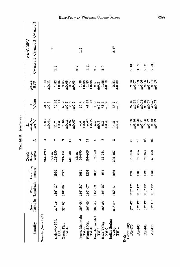
For each site, the principal elements of the heat-flow calculation are given in Tables 1 through 8. Each table c,onsists of twelve col- umns. The first four columns identify the lo- cation of the site by name, hole, or well num- ber (where appropriate), latitude and longitude to the nearest minute, and surface elevation. Column 5 gives the depth range applicable for each line of the table. The columns headed N

and K refer to the number of c,onductivity specimens and the arithmetic mean conduct- tivity (--4- standard error), respectively. If most conductivities in a given set were obtained by measurements on solid disks with the divided-

bar apparatus, the average conductivity is not flagged in any way. The superscripts /• and n in the K column denote that the majority of

6384 SAss •T A•..

.• o o o o

HEAT FLOW IN WESTERN UNITED STATES 6385

6386 SAss

• o o o o o

c• • • o

HEAT FLOW IN WESTERN UNITED STATES 6387

.,-•

.,-•

.,-•

6388 SAss

o

•D

0

. ,..,•

0

HEAT FLOW IN WESTERN UNITED STATES 6389

0

6390 SAss rT ,•.

HEAT FLOW IN WESTERN UNITED STATES 6391

6392 SAss ET AL.

I-IEAT FLOW IN WESTERN UNITED STATES 6393

c•

o o o

•'• t--.,. o0

• o

6394 S•ss •? •.

o c• oo

o oo oo •

I-IEAT FLOW IN WESTERN UNITED STATES 6395

6396 SASS •T A•..

HEAT FLOW IN WESTERN UNITED STATES 6397

6398 SAss

HEAT FLOW IN WESTERN UNITED STATES 6399

ß

-H -H -H -H -H

0 C'q 0 0'• 0

o o o o

6400 SAss •T

o o o

o o o

HEAT FLOW IN WESTERN UNITED STATES 6401

conductivities in that particular data set were is given below all the others, representing the measured on fragments or by the needle probe, best estimate of the heat flow in the area. This respectively (see section on conductivity, is generally the mean (weighted by the length above). of the applicable depth interval) of all holes,

The gradient I' (column 8) is represented in but this can be altered by local factors. For three different ways, depending on which of example, the average q from eight h, oles near the following methods of heat-flow reduction Cedar City, Utah (see Table 8), is about 2.1. was used: There is, however, a strong suggestion of sam-

1. If there was conductivity stratification pling bias toward silicie rocks in some of the on a scale ,of 50 meters or larger, .one line of heterogeneous sedimentary formations. Sam- the table is devoted to each stratum. I' is the pling was not a problem in the Homestake lime- least-square temperature gradient (4- standard stone, a dense, marine limestone formation. error) over the depth range indicated (column Here, 24 component heat flows calculated by 5), and the uneorrected heat flow q(unc), the interval method were tightly grouped about column 9, is the product of this gradient. and a mean of 1.88 4- 0.04, and this value was the mean conductivity (column 7).

2. If conductivity stratification was on a smaller scale, then the heat flow for each of the layers is determined as in 1, and their weighted mean for the depth range indicated (column 5) is entered in column 9. For con- sistency, the arithmetic mean conductivity (and its standard error) for the entire depth range is entered in column 7, and the gradient con- sistent with that conductivity and the heat flow (column 9) is entered in column 8. This derived gradient is shown in parentheses with a superscript i (for interval method).

3. In inhomogeneous materials in which the conductivity stratification is not clearly de- fined, the resistance integral technique of Bull- ard [1939] was used to determine q(unc). As in method 2, a derived gradient consistent with K (column 7) and q(unc) (column 9) is

adopted for the area.

I)ISCUSSION

The foregoing tables contain about 150 new heat-flow determinations representing roughly 100 distinct sites separated from one another by at least a few kilometers. As this more than doubles the published heat-flow data from the western United States, it is worth looking briefly at the present status of the observa- tions. Interpretive studies of these data and additional results being obtained in such key areas as the Klamath Mountains are under

way, and they will be reported separately. Figure 3 distinguishes between the locati. ons

of heat flows reported herein (squares) and those previously published (triangles). Figure 4 distinguishes between all heat flows with val- ues in the 'low-to-normal' range (defined by q

tered in parentheses in column 8. The gradient < 1.5 HFU) and those 'higher than normal' entry has the superscript b (for Bullard (defined by q > 1.6 HFU, with all values method) rounded to the nearest 0.1 HFU). It is seen

ß from Figure 3 that the western United States The final three columns headed q(corr) rep- as a whole is still very. poorly sampled. From

resent the best estimate of heat flow with cor- Figure 4 and the histogram, Figure 5, it is seen rections where appropriate and category as- that the heat flow as we now know it is ex- signments according to criteria outlined above. tremely variable and is dominated by higher- In the majority of cases if a correction was ap- than-normal values. That part of the western plied, it was for steady-state topography, but United States to the west of the Great Plains estimates of other sources of disturbance were corresponds to the 'Mesozoic-Cenozoic oregenie sometimes made in evaluating a heat flow and areas' of Lee and Uyeda [1965]. The most re- assigning it to a category. As stated in the cent compilation of 159 values from such areas introduction, detailed documentation for each throughout the world [Lee, 1970] yielded a of the heat-fi, ow determinations in Tables I mean of 1.76 and standard deviation .of 0.58.

through 8 is in preparation. These values are almost identical to those In areas where there were two or more holes shown for the western United States in Figure

within a small area (~10 km•), a single value 5. This tends to confirm Lee's results even

6402 SAss

120 ø

4

I10 o

7

IOOøW

50øN

i ...... 40ø ;

i ,

i ,

i

, ,

i : ,

L '...z.

,

-.{.- :30 ø

Fig. 3. Sketch map of the western United States showing the locations of heat-flow measurements: Triangles, previously published data (see text for references); squares, U.S. Geological Survcy data. The stippled rectangles are shown in greater detail in Figures 6, 8. 10, and 11. The numbers refer to the same physiographic provinces in the corresponding tables.

HEAT F•,ow •N WESTERN UNITEl) STATES 6403

• ***% ,

'.• •.,• ;.q,* . ,•,• .. e•o ß I • ..... _¾ .....

,

0 500 km ! i i ! ! i

I00 ø W

- 50øN

..... 40 ø

-•- 30 ø

Fig. 4. Generalized representation of heat-flow data from the western United States. Stippled areas are characterized by heat flows of 1.b and less; the heavy lines are 1.b HFU contours. The cross-hatched area is characterized by heat flow of 2.5 and greater.

6404 SAss ST AL.

3O

2O

I0

WESTERN UNITED STATES

West of

All Dottot Grectt Pictins

•Number 244 226

Mectn (hfu) 1.76 1.79

Sfd. de v. 0.61 0.62_.

1.0 2.0 3.0 4.0

q(hfu)

Fig. 5. Itistogram of all heat-flow determinations Jn the western United States. Values greater than 4 HFU were omitted from the analysis.

though almost 100 values are common to both the Sierra Nevada-Great Valley-Coast Range analyses. area of California shown in Figure 6.

From the simple binary division of heat-flow The semicontinuous band of lower heat fl,ows values in Figure 4, it is clear that heat flow paralleling the west coast and its gross relation from the western United States need not be to the San Andreas transform fault system in treated as a homogeneous population. This fact California suggest explanations in terms of has, of course, been recognized for some time, lithospheric subduction and related tectonic and many of the features in Figure 4 have processes [see e.g., Blackwell and Roy, 1971; been identified by Roy et al. [1971] from pre- Roy et al., 1971]. These models are sensitive viously published data. Although the predomi- to assumptions regarding the magnitudes and nant heat flow in the western United States distribution in time and space of the opposing seems to be higher than normal, several re- effects of cooling by descending plates and heat- gions of lower heat flow with lateral dimensions ing by friction, compression, radioactivity, and an order of magnitude greater than crustal ascending melts. Our present ignorance of the thickness can be identified (stippled areas, Fig- mechanics of these processes permits a broad ure 4). The heavy dashed lines enclosing these range of assumptions and a wide variety of regions (Figure 4)represent a preliminary in- explanations of the heat-flow pattern. It is terpretation of the 1.5 HFU contour. (It is of hoped that work in progress at several institu- some interest to note the general coincidence tions will increase the heat-flow coverage of of this cont•our and the lines enclosing the re- this region sufiqciently to obtain more useful gion of intermediate crustal seismic velocity in constraints for models of the continental mar- Figure 2, Pakiser and Zietz [1965].) More re- gin. fined contouring is probably warranted only in One region of conspicuously high heat flow

HEAT FLOW IN WESTERN UNITED STATES 6405

ß

ß

/ SAN FRANCISCO

• 36 ø ß

x O- 0.50

0 0.51- 1.00

•1-1 1.01- 1.50 ß 1.51 - 2.00

ß > 2.00

/ 1200W

•-..• .... •OKM 34"

120 ø

Fig. 6. Heat-flow values in ceniral California and western-central Nevada. (See Figure 3 for location.) Contour interval, 0.5 HFU. The offshore measurements are from Foster [1962] and Burns and Grfm [1967]. The strippied area is the Fran- ciscan block; shaded areas, the Sierra Nevada and Salinian blocks.

occurs in north-central Nevada (cross hatching, Figure 4). The boundaries of this regi, on, and possibly others as yet undetected, could be de- lineated by more systematic heat-flow coverage. This could provide useful guidance in the search for economically exploitable geothermal fields.

Some comments on the status of observa-

tions in the individual provinces follow. Cali/o•'nia co, as•al province (Table 1). This

province includes such diverse physiographic regions as the great Central Valley, the Coast Ranges, the peninsular ranges, and the Los Angeles basin. The range of heat flow reflects the heterogeneity of the province.

Heat flow is high in the Franciscan terrane in the vicinity of San Francisco. Bay, where all values are around 2.0, irrespective of distance from the major strike-slip faults. This is con- sistent with measurements farther south by Brune e• al. [1969], and Henyey [1968], which showed no significant heat-flow anomalies as- sociated with strike-slip faults in California.

The numerous hot springs in the Coast Ranges north of the San Francisco Bay area up to Clear Lake at about latitude 39øN [IVaring, 1965] indicate that the band of high heat flow extends northwestward at least that far. North

of Clear Lake, heat flow seems high near the coast but decreases inland t•o a normal value

near the eastern limit of Franciscan rocks (Fig- ure 6). The measurements along the western margin of the Central Valley are low to normal, consistent with the earlier result of Benl•eld [1947] near Bakersfield. Measurements in the Los Angeles basin and near Santa Ana indicate a region of high heat flow there (Figure 4).

Sie•'ra Nevada (Table 2). With seven meas- urements less than 0.75 HFU, the western margin of the Sierra Nevada is now one of the best documented areas of low heat flow on the

continents. This finding came as a surprise to many because of the observed masses of granite that were thought to contain sufficient heat sources to account for much higher heat flows. It is consistent, however, with low values re- ported from the ocean side of circum-Pacific granitic rocks in Chile [Dimen• e• al., 1965], Amchitka Island [Sass and Mun•'oe, 1970], and northeastern Honshu Island [Uyeda and Horai, 1964] in what might be related tectonic set- tings. Theoretical considerations indicate that the paradox results primarily from anomalously low heat flow from the mantle underlying the Sierra Nevada province and secondarily from the low heat production of granitic rocks in the western part of the Sierra [Roy e• al., 1968b; Lachenb•'uch, 1968a, 1970]. It now ap- pears that the mantle (or deep crustal) heat flow in the Sierra (0.4 HFU) is only about half that characteristic of stable regions and less than one-third that of the Basin and Range province to the east. The increase in heat flow eastward to the Sierra crest (Figure 6) seems generally to correspond to an increase in crustal heat production. The transition at the Basin and Range boundary is discussed in a later paragraph.

Physiographically, the Tehachapi Mountains are the southern 'toe' of the Sierra Nevada.

They are, however, different from the Sierra with respect to structure, origin, and geological history [Bulwalda, 1954].

Many holes were drilled by the California Division of Water Resources along the pro-

6406 SAss • A•.

posed route for the California aqueduct sys- tem. Suitable temperatures were measured in four of the holes, and heat flows are listed in Table 2b. For DH 43 and DH 65, the heat flows are in reasonable agreement with later meas- urements in the same holes by Henyey [1968]. The Tehachapi range appears to provide a thermal as well as a physiographic boundary between the San Joaquin Valley (low-to-nor- mal heat flow) and the Mojave block of the Basin and Range province, which is probably characterized by higher-than-normal heat flow (Figures 4 and 6).

Pacific Northwesi coasial province. Table 3 presents one of the first reliable estimates of heat flow from this province. This low value near Chehalis, Washington, raises the possibil- ity that the crustal heat production in the area is low or, alternatively, that this province is similar to the Sierra Nevada, having a very low heat flow from the mantle. Intrusive rocks

were not encountered at Chehalis, and they are rare in the area. Where Tertiary intrusive rocks are seen, they are marie sills of gabbro or ba- salt porphyry [see e.g., Snavely ei al., 1958; Henriksen, 1956]. H. C. Wagner and P. D. Snavely, Jr., reported in 1966 that the pre- Tertiary crystalline basement of western Wash- ington (not exposed in the Chehalis area) is principally gneissic amphibolite and quartz dio- rite (in unpublished report of U.S.C.ongres- sional Committee on Interior and Insular Af-

fairs, 89th Congress, 2nd Session, pp. 37-46). Thus the small amount of information available

on deep crustal composition indicates a rather marie crust containing few radiogenic heat sources, an observation consistent with the low observed heat flow and a moderate heat flow from the mantle.

Columbia Plaleaus. Largely on the basis of observed volcanism, hot spring activity, and seismicity, Blackwell [1969] included the Co- lumbia Plateau in his postulated 'Cordilleran Thermal Anomaly Zone' (CTAZ) of high heat flow. From the present results (Table 4) it ap- pears that at least the western part of the plateaus may be part of a province of low-to- normal heat flow (see also Figure 4). A single high value from northeastern Nevada supports the assumption that the Snake River Plain is part of the CTAZ (Figure 4).

The Colorado Plateau (Table 5). A heat

f}ow of 2.01 was obtained near the eastern

boundary of the plateau. This high value is con- sistent with the findings of Decker [1969, and personal communication] in this part of the plateau and the neighboring southern Rocky Mountains, and with the suggestion [Edwards• 1966] that this part of the plateau is under- lain by granitic rocks. In the northern part of the plateau, five new sites give normal values with only one (category 3) value as high as 2 (Figures 3 and 4). This part of the plateau evidently is underlain by a Precambrian sedi- mentary terrane [Edwards, 1966]. Low heat flow in the northern Colorado Plateau is also

consistent with Porath's [1971] interpretation of the depth to an electrically conductive layer in this region on the basis of observed magnetic variation anomalies.

Rocky Mouniain province (Table 6). A value of 2.3 was measured in the Galena mine

near Wallace, Idaho, confirming the high values measured by Blackwell [1969] slightly to the east. The five estimates of heat flow from the

central Rocky Mountains are all in the range 1.3 to 1.6 HFU. The high value measured at Denver is included in the Rocky Mountains even though Denver is physiographically part of the Great Plains. This is higher than the nearest neigboring point, Decker's [1969] value of 1.52 at Golden, but. it is consistent with the general pattern of high heat flow in the south- ern Rocky Mountains.

Greai Plains province (Table 7). The only heat-flow estimates made in the Great Plains

during this work were at three sites in the Black Hills of South Dakota and one near

Lyons, Kansas (not shown in Figures 3 and 4). The Black Hills values show a very large varia- tion over a relatively small area, and none is in category 1. The hole at Dacy (which agrees with Blackwell's [1969] estimate at Lead) had been completed only 10 days before the tem- perature measurements were made, and there was evidence of residual drilling disturbances in the temperature profile. Water was flowing slowly but steadily from the collars of both holes from which heat flow is low. Examination

of the temperature profiles (Figure 7), how- ever, indicated no vertical water movement be- low the zone of influx of the Artesian flow, and the vertical temperature profiles below these points were linear and mutually consistent. The

I-IEAT 17LOW IN WESTERN UNITED STATES 6407

low heat flows may well be the result of some fairly deep seated regional hydrologic effect of long duration that has, in effect, thermally de- coupled the rocks penetrated by these holes from the earth below. On the other hand, the possibility that the high heat flows at Lead and Dacy are the result of some local anomalous situation cannot be ignored. We do not have enough information to define a regional heat flow for the Black Hills.

Basin and Range province (Table $). The majority of the data presented in this paper are from the Basin and Range physiographic province, and they generally confirm that this province is one of high heat flow (Figure 4). In addition, however, the new data define some distinct subprovinces, and they place further constraints on the nature of the transition be-

tween the Sierra Nevada and the Basin and

Range provinces. Tucson area. A detailed examination of the

15 heat-flow determinations in a 100 km • area near Tucson serves to illustrate some of the

problems of measuring heat flow in the Basin and Range province and to emphasize that even a 'first-rate' single determination in a region of unknown, complicated structure can be a poor indicator of the actual regional heat flux.

Our six values in this region are all in cate- gory 1, and, from the information given in their table, it appears that all the values of Roy et al. [1968b] are also in this category. There is, however, a spread of nearly a factor of 2 be- t.ween the extreme values (Figures 8 and 9 and Table 9). Despite the variation within each set of determinations, the mean heat flow deter- mined from one set is not significantly different from that calculated from the other (see Table 9).

The structural complexity and the range of heat-flow values encountered in this region are similar to those encountered at Mr. Isa, Queens- land, by Hyndman and Sass [1966]. In the present instance, even though the general struc- ture of the region is well known from drilling and mining operations, there is insu•cient knowledge of detailed structure t.o make the necessary corrections. The combination of steeply dipping beds of contrasting conductivity and ubiquitous faults on every scale probably results in a 'worst case' situation in this region, and several holes are needed to arrive at a re-

100

200 -

I-- _

• 500-

_

400 -

_

500 -

I '" I ' +

ß

ß

ß

ß

ß

ß

+NBH-I

'NBH-2

i

+

+

+

..i.

+

+

+

+

+

ß +

+

ß + +

+

ß + ß

ß +

%+

+

+

+

+

+

+

+

+

+

+

+

+

+

TEMPERATURE, øC

+

+

+

+

+

+

Fig. 7. Temperature profiles from Windy flats (NBH-1) and Moonshine gulch (NBH-2), South Dakota. See Table 7.

liable estimate of regional heat flux. The coef- ficient of correlation between q and K is about 0.23 (Figure 9), a value typical of many found by Horai and Nut [1970] on a larger scale. This poor correlation implies a complicated sit- uati. on that cannot be resolved by simple geo- metrical refraction models even on a scale as

small as that illustrated in Figure 8. Subprovinces in the Basin and Range. Most

heat-flow values in this province are in the range 1.5 to 2.5 HFU. There are some isolated very high and low-to-normal values that are most probably related to local hydrologic con- ditions. In addition, however, there are clusters of consistently high or low values of regional extent for which we must seek more deep- seated causes. From the present work, we de- fine the 'Battle Mountain high' (Figure 10) and the 'Eureka low' (Figure 11). There is also a single category-1 datum of 1.3 I-IFU near Eagle

6408 SASS ET AL.

I'1 ø 15' 110"'30'

3•.Ol5 '-

KCL-7 2. 0 I0 •.OKM i i i

1> M•SS•ON [ - 32.00' ß 2.14 {2.12)

ß •.9•1 (I.93) ß •. lot2 01).

•. •1'.88((.79) 1.5 6 (I.53) HELVETIA

Sierritcl C•.ONTINENTAL • Mrs 2.0 I. • Sonto. Rita Mrs ß

•..05

31' 4 5'

Fig. 8. Heat flows near Tucson, Arizona (see Figure 3 for location). Triangles, values from Roy et al. [1968b]' squares, U.S. Geological Survey values. The values in parentheses were calculated in the same way as those of Roy et al.

3.0

2.5

2.0

I I I

Roy et •tl. [•968• ß USGS +

+ 1.5 I I I

6 7 8 9

Conductivity (m cctl/cm sec øC)

Fig. 9. Heat flow versus mean conductivity for the locations shown in Figure 8.

HEAT FLOW Z• WESTER• U•n•ED S•A•s

TABLE 9. Mean Heat Flows in HFU for the Region South and West of Tucson, Arizona (Range of individual values, 1.56 to 2.97)

64O9

Total Length,* Source of Data Number of Holes meters Average Heat Flow Standard Error

Present work 6 1400 2.04 0.13 Roy et al. [1968b] 9 1430 2.15 0.12 Present work and Roy et al. 15 2830 2.10• 0.09

[1968b] Present work and Roy et al. 15 2830 2.125 0.06

[1968b]

* This includes only those parts of the holes for which temperatures were used to calculate heat flow. I Simple average of all values. •: Mean weighted according to the length of individual holes.

Mountain, California (in the Mojave Block), which may form part of a region of normal heat flow.

It is interesting that there are no thermal springs near Eagle Mountain and that within the Eureka low the thermal springs are less common and are cooler than in the surround- ing areas [see Waring, 1965]. By contrast, the Battle Mountain high contains a fairly dense, regular distribution of warm-to-hot-water springs including the well-known Beowawe geysers (Figure 10).

The high mean heat flow from the Basin and

Range province has been interpreted in terms of near-melting conditions in the lower crust and upper mantle [see e.g. Roy and Blackwell, 1966; Roy et al., 1968b, 1971; Lachenbruch, 1970], and it seems reasonable to interpret the Battle Mountain high as a transient effect of fairly recent crustal intrusion. This view is sup- ported by evidence of Quaternary volcanism within the region [see e.g., Roberts, 1964].

Figure 11 shows a large area north of Las Vegas, which we have called the 'Eureka low,' characterized by heat flows in the range of 0.7 to 1.5 HFU. (The relatively high value of 1.9

ii'so I

116øW

ß WINNEMUCCA

AdelQide m5.4

Elder CreekS.2m eBATTLE MTN

Buckingh(•m ?_.7m 2.1> m5 5 Iron Co. nyon

Po. nther C(•nyon m3-B ß BEOWAWE

L•.nd. er 50m

m5.5 Ten(•bo • 5m Gold Acres

41øN - mi.7

>25 - 0 50 KM 400

I I I I, m J

I I

Fig. 10. Heat flows within the 'Battle Mountain high' (see Figure 3 for location). The symbols are as in Figure 8.

6410 SASS ET AL.

117 ø 0.915 EUREKA 115øW

-39ON

11-8

$TONOPAH

2'0• 1'4.

•1.2 ß (t.5)m

•!.3

ß !'5

1.8 ß eELY

2-1 ß 5.3ß

!.83ß

i•11 2'3 GOLDFIELD

TEMPIUTE

I-5j

j 1.0 •1.9

_ 37 ø O• 1.6B B?...2

/ /

SCALE I I I- i

2.0 &lB 1'72 1-74B e--

PIOCHE

I

50 km

ßMERCURY

B2.2 I i i

Fig. 11. lieat flows between Mercury and Eureka, Nevada (see Figure 3 for location); the heavy line is a 1.5-HFU contour defining the 'Eureka low.' Symbols are as in Figure 8.

near the southern end of the Eureka low was measured in dolomite near a contact with vol-

canic rocks and may be caused, in part, by refraction.) This large apparent anomaly in the normally 'hot' Basin and Range may be in- terpreted in at least two ways. It could repre- sent a systematic hydrologic effect of regional extent or it might be a region where tempera- tures in the lower crust and upper mantle have been below the solidus for some time. How-

ever, the abrupt transitions on the margin of the feature (Figure 11) favor a fairly shallow origin for the anomaly. Our fragmentary tem- perature data from very deep holes in south- ern Nevada suggest an explanation in terms of

systematic though complex interbasin ground water flow with appreciable vertical velocity components to depths of about 3 km (,--1 km below sea level). The identification of such flow patterns is, of course, fundamental to an understanding of the hydrology of this large arid area [see e.g. Winograd and Thordarson, 1968]. It is also fundamental to the evaluation of regional heat-flow analyses, since the con- duerive flux determined in the upper kilometer is usually identified tacitly with .heat loss from the earth's interior. It is seen (Table 8) that several heat flows in the Eureka low have been

assigned to the 'highest quality' category (1) on the basis of usually applied criteria of in-

I-IEAT FLOW IN WESTERN UNITED STATES 6411

ternal consistency. Only under exceptional cir- cumstances will supplementary information be available to reveal the possible occurrence of deep-seated 'hydrologic decoupling' on a re- gional scale.

The Sierra Nevada-Basin and Range transi- tion. Roy and Blackwell [1966] and Roy et al. [1968b, 1971] have concluded that the transition between these two provinces takes place over a short distance (on the order of 100 km) within the Basin and Range province. Data now available suggest a more abrupt transition that might extend into the eastern Sierra Nevada.

Figure 6 shows all the previously published data along the transition together with the present results. The most striking increase in heat flow is that between Gardnerville (GV) and the Pine Nut Canyon (PN). If equal weight is given to the two values, then we must conclude that the transition occurs within 20

km. North of these points the new data firmly establish high heat flow between Carson City and Reno, only 15 to 20 km from the physio- graphic boundary of the Sierra province. Al- though independent evidence [Becker, 1882] indicates that the very high heat flows near the Comstock lode are from local hydrologic effects, no such effects are evident at Washing- ton Hill (WH), Silver City (SC), or Pine Nut Canyon (PN) (Figure 6). Measurements at Black Rock and Deep Spring 150 km to the south, (10 and 35 km from the physiographic boundary), also indicate high heat flow extend- ing very close to the edge of the Basin and Range province.

As previously mentioned, interpretive studies suggest that the thermal transition from the Basin and Range province to the Sierra Nevada might involve a change in heat flow from the deep crust or mantle by a factor of 3. Such a transition would be extremely dimcult to ex- plain by almost any model if it occurred over a lateral distance of only 10 or 20 km (a situa- tion that must exist if we assume that the

transition zone is in the Basin and Range province). It therefore seems probable that, like the Basin and Range faulting, the heat- flow transition extends into the eastern Sierra.

This view is supported by recent heat-flow re- sults from Lake Tahoe presented by Lee and Henyey [1970].

Acknowledgments. We are greatly indebted to many individuals connected with the mining and petroleum industries, without whose willing help the majority of the determinations presented here would not have been possible. We are grateful to other governmental agencies, in particular the Atomic Energy Commission, the Bureau of Mines, the Bureau of Reclamation, and the California Division of Water Resources, for allowing access to their boreholes. Many colleagues in the U.S. Geological Survey were very helpful in supplying information on regional and local geology and in arranging access to exploratory borings in their areas. We thank R. F. Roy for kindly giving us a preprint of Roy et al. [1971] and for allowing us to cite the manuscript. John Tanida and Ming Ko rendered valuable assistance in the processing of the vast number of primary data. G. Brent Dalrymple, William H. Diment, William B. Joyner, and Donald E. White read the manu- script and offered valuable comments.

Publication has been authorized by the Direc- tor, U.S. Geological Survey.

t•EFERENCES

Beck, A. E., Techniques of measuring heat flow on land, in Terrestrial Heat Flow, Geophys. Monogr. Set., vol. 8, edited by W. H. K. Lee, pp. 24-57, AGU, Washington, D.C., 1965.

Becker, G. F., Geology o/ the Comstock Lode and the Washoe District, U.S. Geol. Surv. Monogr. 3, 422 p p., 1882.

Benfield, A. E., A heat flow value for a well in California, Amer. J. Sci., 245, 1-18, 1947.

Birch, Francis, Temperature and heat flow in a well near Colorado Springs, Amer. J. Sci., 245, 733-753, 1947.

Birch, Francis, The effects of Pleistocene climatic variations upon geothermal gradients, Amer. J. Sci., 246, 729-760, 1948.

Birch, Francis, Flow of heat in the Front Range, Colorado, Geol. Soc. Amer. Bull., 61, 567-630, 1950.

Birch, Francis, The present state of geothermal investigations, Geophysics, 19, 64•%-659, 1954.

Birch, Francis, and Harry Clark, The thermal con- ductivity of rocks and its dependence on tem- perature and composition, Amer. J. Sci., 238, 529-558 and 613-635, 1940.

Birch, Francis, R. F. Roy, and E. R. Decker, Heat flow and thermal history in New England and New York, in Studies o/ Appalachian Ge- ology: Northern and Maritime, edited by E-an Zen, W. S. White, J. B. Hadley, and J. B. Thompson. Jr., pp. 437-451, Interscience, New York, 1968.

Blackwell, D. D., Heat-flow determinations in the northwestern United States, J. Geophys. Res., 74, 992-1007, 1969.

Blackwell, D. D., and R. F. Roy, Geotectonics and Cenozoic history of the western United States (abstract), Geol. Soc. America, Cordil-

6412 SAss ET A•,.

leran Sect., 67th Annu. Meet., Riverside, Calif., 1971, Abstr. Programs, 3, 84-85, 1971.

Bredehoeft J. D., and I. S. Papadopulos, Rates of vertical groundwater movement estimated from the earth's thermal profile, Water Resour. Res., 1, 325-328, 1965.

Brune, J. N., T. L. Henyey, and R. F. Roy, Heat flow, stress, and rate of slip along the San Andreas fault, California, J. Geo•hys. Res., 74, 3821-3827, 1969.

Bullard, E. C., Heat flow in South Africa, Proc. Roy. Soc. London, Ser. A, 173, 474-502, 1939.

Bullard, E. C., The time necessary for a borehole to attain temperature equilibrium, Mon. Not. Roy. Astron. Soc., Geophys. Suppl., 5, 127-130, 1947.

Burns, R. E., and P. J. Grim, Heat flow in the Pacific Ocean off central California, J. Geophys. Res., 72, 6239-6247, 1967.

Buwalda, J.P., Geology of the Tehachapi Moun- tains, California, in Geology o[ Southern Cali- fornia, edited by R. H. Jahns, Calif. Dep. Natur. Resour. Div. Mines Bull., 170(6), 131-142, 1934.

Clark, S. P., Jr., Heat flow at Grass Valley, Cali- fornia, Eos Trans. A GU, 38, 239-244, 1957.

Combs, J. B., Terrestrial heat flow in north central United States, Ph.D. thesis, Massachusetts In- stitute of Technology, Cambridge, 1970.

Costain, J. K., and P.M. Wright, Heat flow and geothermal measurements in Utah (ab- stract), Eos Trans. A GU, 49, 325, 1968.

Decker, E. R., Heat flow in Colorado and New Mexico, J. Geophys. Res., 74, 550-559, 1969.

Diment, W. H., Francisco Ortiz O., Louis Silva R., and Carlos Ruiz F., Terrestrial heat flow at two localities near Vailchar, Chile (abstract), Eos Trans. AGU, 46, 175, 1965.

Edwards, Jonathan, Jr., The petrology and struc- ture of the buried Precambrian basement of

Colorado, Quart. Colo. School Mines, 61(4), 436 pp., 1966.

Fenneman, N.M., Physiographic divisions of the United States, Ann. Ass. Amer. Geogr., 18, 261- 353, 1928.

Foster, T. D., Heat-flow measurements in the northeast Pacific and in the Bering Sea, J. Geo- phys. Res., 67, 2991-2993, 19,62.

Henriksen, D. A., Eocene stratigraphy of the lower Cowlitz River-eastern Willapa Hills area, south- western Washington, Wash. Dep. Conserr. Div. Mines Geol. Bull., 43, 122 pp., 1956.

Henyey, T. L., Heat flow near major strike-slip faults in central and southern California, Ph.D. thesis, California Institute of Technology, Pasa- dena, 1968.

Herrin, Eugene, and S. P. Clark, Jr., Heat flow in west Texas and eastern New Mexico, Geo- physics, 21, 1087-1099, 1956.

Horai, Ki-iti, and Amos Nur, Relationship among terrestrial heat flow, thermal conductivity, and geothermal gradient, J. Geop,hys. Res., 75, 1985- 1991, 1970.

Howard, L. E., and J. H. Sass, Terrestrial heat

flow in Australia, Y. Geophys. Res., 69, 299- 308, 1964.

Hyndman, R. D., and J. H. Sass, Geothermal measurements at Mount Isa, Queensland, J. Geophys. Res., 71, 587-601, 1966.

Jaeger, J. C., The effect of the drilling fluid on temperatures measured in boreholes, J. Geo- phys. Res., 66, 563-569, 196,1.

Jaeger, J. C., Application of the theory of heat conduction to geothermal measurements, in Terrestrial Heat Flow, Geophys. Monogr. Ser., vol. 8, edited by W. H. I(. Lee, pp. 7-23, AGU, Washington, D.C., 1965.

Jaeger, J. C., and J. H. Sass, Lee's topographic correction in heat flow and the geothermal flux in Tasmania, Geofis. Pura Appl., 54, 53-63, 1963.

Jaeger, J. C., and R. F. Thyer, Report on progress in geophysics: Geophysics in Australia, Geo- phys. Y., 3, 450-461, 1960.

Kraskovski, S. A., On the thermal field in shields, Izv. Akad. Nauk. SSSR, Ser. Geofiz., 247-250, 1961.

Lachenbruch, A. H., Three-dimensional heat flow in permafrost beneath heated buildings, U•S. Geol. Surv. Bull. 1052-B, 51-69, 1957a.

Lachenbruch, A. H., Thermal effects of the ocean on permafrost, Geol. Soc. Amer. Bull., 63, 1515- 1529, 1957b.

Lachenbruch, A. H., Preliminary geothermal model of the Sierra Nevada, Y. Geophys. Res., 73, 6977-6989, 1968a.

Lachenbruch, A. H., Rapid estimation of the topographic disturbance to superficial thermal gradients, Rev. Geophys. Space Phys., 6, 365- 400, 1968b.

Lachenbruch, A. H., Crustal temperature and heat production: Implications of the linear heat-flow relation, Y. Geophys. Res., 75, 3291-3300, 1970.

Lachenbruch, A. H., and M. C. Brewer, Dissipa- tion of the temperature effect of drilling a well in arctic Alaska, U.S. Geol. Surv. Bull. 1083-C, 73-109, 1959.

Lachenbruch, A. H., and B. V. Marshall, Heat flow through the Arctic Ocean floor: The Can- ada basin-Alpha rise boundary, J. Geophys. Res., 71, 1223-1248, 1966.

Lachenbruch, A. H., and B. V. Marshall, Heat flow in the Arctic, Arctic, 22, 300-311, 1969.

Lachenbruch, A. H., M. C. Brewer, G. W. Greene, and B. V. Marshall, Temperatures in perma- frost, in Temperature--Its Measurement and Control in Science and Industry, edited by C. M. Herzfeld, vol. 3, pp. 791-803, Reinhold, New York, 1962.

Lachenbruch, A. H., H. A. Wollenberg, G. W. Greene, and A. R. Smith, Heat flow and heat production in the central Sierra Nevada, pre- liminary results (abstract), Eos Trans. AGU, 47, 179, 1966.

Lee, T. C., and T. L. Henyey, Heat flow in Lake Tahoe, California-Nevada (abstract), Eos Trans. A GU, 51, 824, 1970.

Lee, W. H. K., On the global variation of terres-

I-IEAT FLOW IN WESTERN UNITED STATES 6413

trial heat flow, Phys. Earth Planet. Interiors, 2, 332-341, 1970.

Lee, W. H. K., and Seiya Uyeda, Review of heat flow data, in Terrestrial Heat Flow, Geophys. Monogr. Ser., vol. 8, edited by W. H. K. Lee, pp. 87-190, AGU, Washington, D.C., 1965.

Pakiser, L. C., and Isidore Zietz, Transcontinental crustal and uppermantle structure, Rev. Geo- phys. Space Phys., 3, 505, 1965.

Porath, H., Magnetic variation anomalies and seismic low-velocity zone in the western United States, J. Geophys. Res., 76, 2643, 1971.

Ratcliffe, E. H., Thermal conductivities of fused and crystalline quartz, Brit. J. Appl. Phys., 10, 22-28, 1959.

Roberts, R. J., Stratigraphy and structure of the Antler Peak quadrangle, Humboldt and Lander counties, Nevada, U.S. Geol. Surv. Pro[. Pap. 459-A, A1-A93, 1964.

Roy, R. F., Heat flow measurements in the United States, Ph.D. thesis, Harvard University, Cam- bridge, Mass., 1963.

Roy, R. F., and D. D. Blackwell, Heat flow in the Sierra Nevada and western Great Basin (ab- stract), Eos Trans. AGU, 47, 179-180, 1966.

Roy, R. F., D. D. Blackwell, and Francis Birch, Heat generation of plutonic rocks and con- tinental heat flow provinces, Earth Planet. Sci. Lett., 5, 1-12, 1968a.

Roy, R. F., E. R. Decker, D. D. Blackwell, and Francis Birch, Heat flow in the United States, J. Geophys. Res., 733, 5207-5221, 1968b.

Roy, R. F., D. D. Blackwell, and E. R. Decker, Continental heat flow, in The Nature o/ the Solid Earth, edited by E. C. Robertson, McGraw-Hill, New York, in press, 1971.

Sass, J. H., and R. J. Munroe, Heat flow from deep boreholes on two island arcs, J. Geophys. Res., 75, 4387-4395, 1970.

Sass, J. H., P. G. Killeen, and E. D. Mustonen, Heat flow and surface radioactivity in the Quirke Lake syncline near Elliot Lake, Ontario, Canada, Can. J. Earth Sci., 5, 1417-1428, 1968a.

Sass, J. H., A. H. Lachenbruch, G. W. Greene, T. H. Moses, Jr., and R. J. Munroe, Progress report on heat-flow measurements in the western United States (abstract), Eos Trans. AGU, •9, 325-326, 1968b.

Sass, J. H., R. J. Munroe, and A. H. Lachenbruch, Measurement of geothermal flux through poorly consolidated sediments, Earth Planet. Sci. Lett., 4, 293-298, 1968c.

Sass, J. H., A. H. Lachenbruch, and R. J. Munroe, Thermal conductivity of rocks from measure- ments on fragments and its application to heat- flow determinations, J. Geophys. Res., 76, 3391- 3401, 1971.

Snavely, P. D., Jr., R. D. Brown, Jr., A. E. Roberts, and W. W. Rau, Geology and coal resources of the Centralia Chehalis district, Washington, U.S. Geol. Surv. Bull., 1053, 159 pp., 1958.

Spicer, H. C., Geothermal gradients and heat flow in the Salt Valley anticline, Utah, Boll. Geo/. Teor. Appl., 6, 263-282, 1964.

Uyeda, Seiya, and Ki-iti Horai, Terrestrial heat flow in Japan, J. Geophys. Res., 69, 2121, 1964.

Von Herzen, R. P., and A. E. Maxwell, The measurement of thermal conductivity of deep- sea sediments by a needle probe method, J. Geophys. Res., 64, 1557-1563, 1959.

Von Herzen, R. P., and Seiya Uyeda, Heat flow through the eastern Pacific floor, J. Geophys. Res., 68, 4219-4250, 1963.

Walsh, J. B., and E. R. Decker, Effect of pressure and saturating fluid on the thermal conductivity of compact rock, J. Geophys. Res., 71, 3053- 3061, 1966.

Waring, G. A., Thermal springs of the United States •nd other countries of the world, a summary, U.S. Geol. $erv. Pro•. Pap., 492, 1965.

Warren, R. E., J. G. Sclater, Victor ¾acquier, and R. F. Roy, A comparison of terrestrial heat flow and transient geomagnetic fluctuations in the southwestern United States, Geophysics, 34, 463-478, 1969.

Winograd, I. J., and William Thordarson, Struc- tural control of groundwater movement in mi- geosynclinal rocks of south-central Nevada, in Nevada Test Site, Mere. 110, edited by E. B. Eckel, pp. 35-48, Geological Society of America, Boulder, Colo., 1968.

(Received March 22, 1971.)