environments

Article

Hepatobiliary-Related Outcomes in US AdultsExposed to Lead

Emmanuel Obeng-Gyasi 1,*, Rodrigo X. Armijos 2, M. Margaret Weigel 2, Gabriel Filippelli 3 ID

and M. Aaron Sayegh 4

1 Department of Built Environment, North Carolina Agricultural and Technical State University;Greensboro, NC 27411, USA

2 Department of Environmental and Occupational Health, Indiana University School of Public Health,Bloomington, IN 47405, USA; rarmijos@indiana.edu (R.X.A.); weigelm@iu.edu (M.M.W.)

3 Department of Earth Sciences, Indiana University Purdue University Indianapolis;Indianapolis, IN 46202, USA; gfilippe@iupui.edu

4 Department of Epidemiology and Biostatistics, Indiana University School of Public Health,Bloomington, IN 47405, USA; msayegh@indiana.edu

* Correspondence: eobenggyasi@ncat.edu; Tel.: +1-336-285-3132

Received: 28 February 2018; Accepted: 28 March 2018; Published: 31 March 2018�����������������

Abstract: The purpose of this cross-sectional study was to investigate hepatobiliary-related clinicalmarkers in Unites States adults (aged ≥ 20) exposed to lead using the National Health and NutritionExamination Survey (NHANES) 2007–2008 and 2009–2010 datasets. Clinical markers and occupationwere evaluated in 4 quartiles of exposure—0–2 µg/dL, 2–5 µg/dL, 5–10 µg/dL, and 10 µg/dLand over—to examine how the markers and various occupations manifested in the quartiles.Linear regression determined associations, and binary logistic regression predicted the likelihood ofelevated clinical makers using binary degrees of exposure set at (2 µg/dL, 5 µg/dL, and 10 µg/dL).Clinical makers, and how they manifested between exposed and less-exposed occupations, wereexplored in addition to how duration of exposure altered these clinical markers. In regressionanalysis, Gamma-Glutamyl Transferase (GGT), total bilirubin, and Alkaline Phosphatase (ALP) werepositively and significantly associated with Blood lead level (BLL). Using binary logistic regressionmodels, at the binary 2 µg/dL level ALP, and GGT were more likely to be elevated in those exposed.At 5 µg/dL level, it was ALP and GGT that were more likely to be elevated in those exposedwhereas at 10 µg/dL level, it was GGT that were more likely to be elevated in those exposed. In theoccupational analysis, Aspartate Aminotransferase (AST), Alanine Aminotransferase (ALT), GGT,and ALP showed differences between populations in the exposed and less-exposed occupations.Regarding Agriculture, Forestry and Fishing, duration of exposure altered AST, ALP, and totalbilirubin significantly (p < 0.05) while ALT and GGT were altered moderately significantly (p < 0.10).With mining, duration of exposure altered AST and GGT moderately significantly, whereas inconstruction duration in occupation altered AST, and GGT significantly, and total bilirubin moderatelysignificantly. The study findings are evidence of occupational exposure to lead playing a significantrole in initiating and promoting adverse hepatobiliary clinical outcomes in United States adults.

Keywords: lead exposure; hepatobiliary outcomes; heavy metals; occupational exposure

1. Introduction

Lead exposure among adults mainly occurs in the workplace within lead and zinc ore mining,painting, and battery manufacturing industries [1]. Indeed, occupational exposure to inorganiclead in Western countries occurs in mines and smelters, welding of lead painted metal, batterymanufacturing plants, and in the glass manufacturing industry [2]. Exposure to lead can also occur in

Environments 2018, 5, 46; doi:10.3390/environments5040046 www.mdpi.com/journal/environments

Environments 2018, 5, 46 2 of 17

community-based settings as is the case in El Paso, Texas, and Baltimore, Maryland. This is due to thelegacy of leaded gasoline and paint [3,4] in addition to industrial sources of exposure [5].

Lead is toxic and causes many adverse clinical outcomes in adults. It has no role in normalbiological function in humans but through several mechanisms can induce adverse health outcomes,including adverse hepatobiliary outcomes. Furthermore, because lead is environmentally persistent,populations can remain continuously exposed in areas where it was previously used. Sources andextent of lead exposure have fallen dramatically over the past 30 years because of interventions suchas, lead content being reduced in gasoline, lead being limited in household paint, existing sourcesof lead paint being contained, as well as lead being limited in the food canning process and inindustrial emissions and water. Despite that, lead continues to be an issue of public health significancein the United States. It is biologically and environmentally persistent, making it hazardous as itaffects almost every organ system within the human body, including the hepatobiliary system [6–9].Studies on the hepatotoxic effects of lead have demonstrated that exposure to lead alters cholesterolmetabolism, xenobiotic metabolism, and plays a role in hepatic hyperplasia [10]. Oxidative stressis a major mechanism for the pathogenesis of lead induced toxicity. Hsu and Leon Guo [11]determined that lead-induced oxidative stress contributes to the pathogenesis of lead poisoningby disrupting the delicate pro-oxidant/antioxidant balance in the cells of mammals. Indeed, leadexposure causes the generation of reactive oxygen species and modification of antioxidant defensesystems in occupationally exposed workers and animals and thus negatively impacts the liver. Autopsystudies of lead-exposed patients have shown that a significant proportion of absorbed lead is storedin the liver, giving credence to its disproportionate effects in the hepatobiliary system [12]. Studyingmore about its effects on liver injury is thus an issue of public health importance as liver diseasesaffects 3.9 million United States adults and there are 12 deaths per 100,000 people in the United Statesfrom liver disease [13].

Liver and biliary system injury can be evaluated by examining clinical markers of liver damage.Liver function test measuring hepatic enzymes such as Alanine Aminotransferase (ALT), AspartateAminotransferase (AST), Alkaline Phosphatase Test (ALP), and Gamma-Glutamyl Transferase (GGT),in addition to test measuring Total Bilirubin, help to assess the injury status of the liver and gallbladder,but these clinical markers can also be elevated due to pathology in other organs; thus, an appropriatedifferential diagnosis needs to be administered [14].

Aminotransferases are used to detect and monitor the progression and resolution of hepatocellularinjury [15]. AST catalyzes the conversion of aspartate and alpha-ketoglutarate to oxaloacetate andglutamate [16]. AST is synthesized in the liver but is not specific to the liver: the kidney, heart, brain,and muscles cells also synthesize smaller amounts of AST. ALT catalyzes the transfer of an aminogroup to alpha-ketoglutarate from alanine in the alanine cycle, producing pyruvate and glutamatein the process [16]. It is synthesized in the liver and is also usually present in low amounts in theblood. With liver injury ALT tends to rise, as it is more specific to the liver than AST. Gamma-glutamyltransferase (GGT) is a sensitive marker of hepatic inflammation. GGT, an enzyme that functionsin the gamma-glutamyl cycle, catalyzes the transfer of gamma-glutamyl functional groups frommolecules such as glutathione and is found not only in the liver but in other organ tissues, includingthe kidney and pancreas. Elevated GGT levels in serum may indicate various liver pathologies,including fatty liver disease, liver inflammation or hepatitis [17]. It can also be elevated due tocholestasis. Alkaline phosphatase is found throughout the body, including in the liver, kidney, bone,and digestive system, and is a good marker to test for hepatobiliary damage in addition to bonecell dysregulation. Concentration of ALP is generally increased by cholestasis, injury to intestinalepithelium, or damage to the biliary epithelium [16]. Total Bilirubin consists of unconjugated andconjugated bilirubin. Unconjugated bilirubin is formed when heme is released from hemoglobin and isconverted to unconjugated bilirubin, the unconjugated bilirubin is then transported to the liver wherewithin the hepatocytes bilirubin, via a uridine diphosphoglucuronate-glucuronyltransferase (UDP-GT)process, is conjugated with glucuronic acid. This process can be altered by various pathology along

Environments 2018, 5, 46 3 of 17

the pathway. Serum activity of these clinical markers are often a reflection of the physiological state ofthe liver and their activity in blood often indicates the severity of cellular damage [12,14]. The effectsof lead on liver injury was examined in a study that looked at the effects of blood lead on plasmalevels of amino acids and serum liver enzymes among the exposed (100 industrial workers) andcontrols (100-non industrial workers) in which they found liver enzymes to be significantly elevated inindustrialized workers as compared to non-industrialized workers [18].

Adult Blood Lead Epidemiology Surveillance (ABLES) operated under the Centers for DiseaseControl and Prevention (CDC), is a state-based surveillance of adult BLLs in the United States.In 1994, the rate of lead exposure to workers resulting in BLLs ≥ 25 µg/dL was 14 employed adultsper 100,000. In 2011, the rate was 6.4 employed adults per 100,000. The Occupational Safety and HealthAdministration’s (OSHA) lead standards require that workers be removed from lead exposure sourceswhen BLLs ≥ 50 µg/dL in the construction industry or 60 µg/dL in general industry, and in the contextof previous elevated exposure, workers are allowed to return to work when their BLLs are below40 µg/dL [1]. It should be noted that the half-life of lead in blood is 35 days and 30 years in bone [19].Blood lead level (BLL) is a reflection of acute exposure to lead while bone lead is a measure of chronicexposure to lead. Using BLL to measure lead exposure is a validated method in both precision andaccuracy and a better method to test lead levels than urine lead measurements, which, because oflead’s rapid clearance, makes it less accurate. Our study sought to examine the effects of lead on thehepatobiliary system in the US general adult populations.

2. Materials and Methods

2.1. Hypothesis

In this study it was hypothesized that exposure to lead adversely affects hepatobiliary functionsvia adversely affecting liver and biliary enzymes. In that respect this study sought to investigate theeffects of lead exposure on the studied participants by analyzing their AST, ALT, ALP, GGT, and totalbilirubin clinical markers. The analysis of BLLs and clinical markers within a sample of United Statesadults determined the extent to which exposure to lead potentially altered the markers in individuals.Lead’s impact on occupation was also explored to determine its effects on the clinical makers of interestamong those occupationally exposed to lead.

The sociodemographic, behavioral, and anthropometric covariates made it possible to statisticallycontrol for factors associated with adverse hepatobiliary outcomes. It also made it possible to makeestimations about the contribution of lead to studied participants’ hepatobiliary clinical markers.

In all, it was hypothesized that being exposed to lead would be associated with elevated ALT,AST, total bilirubin, ALP, and GGT.

2.2. Study Design

Research Design

Data from NHANES 2007–2010 were used to examine the association between lead andhepatobiliary related markers ALT, AST, ALP, total bilirubin and GGT—in the general United Statesadult population. The NHANES 2007–2010 survey was conducted by the CDC using a representativesample of the U.S. noninstitutionalized civilian population. Altogether, 12,153 adult subjects ≥20 yearswere included in this complex multistage, stratified cluster survey in 2007 through 2010, which afterfactoring in sampling weights represented 217,057,187 people. Of the 12,153 participants, blood leadwas measured in 9781 adult subjects representing an estimated 182,052,299 people. For ALT values,10,992 were measured; this represented 204,454,456 of the population. AST value levels were measuredfor 10,991, representing 204,424,018 of the population whereas GGT value levels were measured for10,996, which represented 204,525,189 of the population. With respect to total bilirubin, the levelsmeasured were for 9397, representing 170,044,349 of the population whereas ALP was measured for10,996 adults, which represented 204,523,110 of the population.

Environments 2018, 5, 46 4 of 17

2.3. Data Collection

Recruitment

In NHANES, participants are selected using a complex sampling methodology with various clinicalmakers collected every year from participants who are representative of the non-institutionalizedpopulation. For this analysis, 4-year weights for individual probabilities drawn from biomarker datasets were used following the NCHS web tutorial (NCHS 2010a). The sample weights for NHANES2007–2010 were based on population estimates that incorporated the national census count. NHANES2007–2010 consisted of a standardized questionnaire administered in the home by a trained interviewerfollowed by a comprehensive physical examination at a Mobile Examination Center (MEC). The dataare freely available from the institution’s homepage.

A cross-sectional study, NHANES collects nationally representative data on health outcomes anddisease. Methods for demographic, clinical and survey data collection can be found at the NCHS’website [20,21].

2.4. Quality Control

2.4.1. For Demographics

The computer-assisted personal interview (CAPI) software, that was used to gather the interviewdata in NHANES 2007–2010, contained data edit and consistency checks which notified the interviewerwhen the recorded data was erroneous. Information screens provided standardized descriptions of theterminology and concepts that were used in the questionnaires for the interviewer. Data collectionwas consistently reviewed by NHANES field officers and subsets of participants were re-contacted toensure accuracy. Finally, several interviews were audio-taped and reviewed by National Center forHealth Statistics (NCHS) and contractor staff to ensure quality.

2.4.2. For Hepatobiliary Markers

The NHANES 2007–2010 quality assurance/quality control (QA/QC) protocols fulfilled the 1988Clinical Laboratory Improvement Act. Detailed instructions regarding QA/QC are found in theNHANES Laboratory/Medical Technologists Procedures Manual (LPM). The General Documentationof Laboratory Data file provides detailed QA/QC protocols.

2.4.3. Biomarkers and Biometric Data in This Study

The major biomarker of interest in this study is blood lead, which is representative of soft tissuelead and a good measure of body burden and internal dose of lead [22]. BLLs can help one determinethe degree of exposure to lead at a snapshot in time. Other biomarkers of interest are AST, ALT,GGT, ALP, and total bilirubin. These are hepatobiliary biomarkers. The hepatobiliary biomarkershave been positively associated with exposure to lead in some studies while others have found noassociation [18,23,24].

2.4.4. Instruments and Procedures

In the study, the biochemistry biomarkers were measured using a Beckman Synchron LX20,Beckman UniCel® DxC800 Synchron (Brea, CA, USA) at Collaborative Laboratory Services and theRoche Modular P chemistry analyzer at the University of Minnesota, MN, USA. Metal assays in wholeblood samples were conducted in the NHANES 2007–2010 at the Division of Laboratory Sciences,National Center for Environmental Health (NCEH) of the CDC. Blood lead was determined byinductively coupled plasma mass spectrometry (ICP-MS; CDC method no. ITB0001A).

Environments 2018, 5, 46 5 of 17

2.5. Data Management

Data management was done in accordance with the NHANES analytical guidelines relating to itssurvey design and weighting [25]. The software Stata SE/15.0 (StataCorp, College Station, TX, USA)was used for data management.

2.6. Analytical and Statistical Approaches

This study analyzed results from adults aged 20 and older. In portions of the study, analysis wasperformed on those experiencing various degrees of exposure represented by BLLs in four quartiles;0–2 µg/dL, 2–5 µg/dL, 5–10 µg/dL, 10+ µg/dL presented in this study as quartile 1, quartile 2,quartile 3, and quartile 4 respectively, which represent thresholds typically and historically used in theliterature to represent elevated exposure. Association between lead and hepatobiliary outcomes wereexplored using linear regression. Since the variables of interest were not normally distributed, naturallog transformation was used for dependent and independent variables in regression analysis.

Both continuous and categorical data were analyzed. For linear regression, all independentvariables were examined as continuous variables. The covariates of interest (gender, BMI, ethnicity,and age), and consumption of alcohol (those who had taken at least 12 alcoholic drinks in the past year)and smoking habits, were adjusted for to determine leads impact on the clinical markers of interest.

In the binary logistic regression models, the dependent variable was categorical for lead exposureat the 2, 5, and 10 µg/dL levels. Statistical analyses were performed using Stata SE/15.0 (StataCorp,College Station, TX, USA) as the software allowed for adjustment for clusters and strata of the complexsample in addition to incorporating the sample weight in order to generate estimates for the totalnoninstitutionalized civilian population of the United States.

In addition, occupational analysis was performed examining the mean difference between theclinical markers of occupationally exposed workers as compared to occupationally less exposedworkers. Finally, the mean levels of the clinical markers of interest were explored in durations of0–5 years, 5–10 years, and over 10 years to see how the markers manifested over various time periods.

A p-value of <0.05 was considered significant while a value of <0.10 was considered moderatelysignificant. Excel 2016 was used to generate charts/figures.

3. Results

3.1. Sociodemographic, Anthropometric and Clinical Variables/Data

The objective of this section is a presentation of the results on lead exposure with regards tothe participant sociodemographic characteristics, and those of their clinical and anthropometricinformation. The results of the sociodemographic information will be presented first. In presenting theresults of participants’ sociodemographic information; gender and ethnicity, as well as their occupationare presented.

3.1.1. Gender

The results (in percentages) of the different gender categories and quartiles of exposure in thestudy data are shown in Table 1 below with the percent standard error (SE%), a measure of the precisionof the mean, shown in brackets. As can be seen, males represent a larger percent of those in the highestexposure groups while females represent a larger percent of the lowest exposure group.

Environments 2018, 5, 46 6 of 17

Table 1. Gender and quartiles of exposure.

Lead Exposure Male% (SE%) Female% (SE%)

N 5858 6295Quartile 1 (0–2 µg/dL) 67.8% (1.2) 82.5% (0.9) ****Quartile 2 (2–5 µg/dL) 27.8% (1.0) ** 16.6% (0.8)

Quartile 3 (5–10 µg/dL) 3.7% (0.3) *** 0.9% (0.1)Quartile 4 (10+ µg/dL) 0.7% (0.2) * 0.1% (0.0)

Total 100% 100%

* p < 0.05 Male making up a significantly larger proportion than Female in this exposure group; *** p < 0.05 Malemaking up a significantly larger proportion than Female in this exposure group; ** p < 0.05 Male making upa significantly larger proportion than Female in this exposure group; **** p < 0.05 Female making up a significantlylarger proportion than Male in this exposure group.

3.1.2. Ethnicity

The ethnic groups identified in the data were Mexican American, Non-Hispanic White,Non-Hispanic Black, Other Hispanic, and Other Race (including multi-racial). Percentages representingthe various quartiles of exposure are shown in Table 2 below. As can be seen, among Mexican-Americans,a larger percentage are in the highest exposure group (quartile 4) as compared to other ethnicgroups. While in the second largest exposure group, Blacks and Mexican-Americans make up a largerpercentage as compared to other ethnic groups.

Table 2. Ethnicity and quartiles of exposure.

Lead Exposure MexicanAmerican% (SE%)

Other Hispanic%(SE%)

Non-HispanicWhite% (SE%)

Non-HispanicBlack% (SE%)

Other Race—IncludingMulti-Racial% (SE%)

N 1032 600 8342 1377 802Quartile 1 72.0% (1.9) 80.7% (2.1) +++ 76.9% (1.2) ***** 71.5% (1.3) 66.7% (3.4)0–2 µg/dLQuartile 2 23.2% (1.4) ++ 17.3% (2.4) 21.1% (1.1) 24.4% (1.2) + 29.7% (2.9) ****2–5 µg/dLQuartile 3 3.7% (0.7) ** 1.6% (0.3) 1.8% (0.2) 3.7% (0.5) *** 2.9% (0.8)

5–10 µg/dLQuartile 4 1.0% (0.3) *,# 0.4% (0.3) 0.2% (0.1) 0.3% (0.1) 0.8% (0.5)10+ µg/dL

Total 100% 100% 100% 100% 100%+p < 0.05 significant difference between Non-Hispanic Black and Other Hispanic and non-Hispanic White; ++ p < 0.05significant difference between Mexican-American and Other Hispanic; +++ p < 0.05 significant difference betweenOther Hispanic and Mexican-American, non-Hispanic Black and Other Race-including multi-racial; * p < 0.05significant difference between Mexican American and Non-Hispanic white; ** p < 0.05 significant differencebetween Mexican American and other Hispanic and non-Hispanic white; *** p < 0.05 significant difference betweennon-Hispanic Black and Other Hispanic, non-Hispanic White; **** p < 0.05 significant difference between other race-including multiracial and Mexican American, Other Hispanic, and non-Hispanic white; ***** p < 0.05 significantdifference between non-Hispanic White and Mexican-American, Non-Hispanic Black and Other Race-IncludingMultiracial; # p < 0.10 moderately significant difference between Mexican American and Non-Hispanic Black.

3.1.3. Occupation

Longevity in Jobs (Occupation One Had Spent the Most Time in)

The longevity of employment in a job was also taken into consideration to see how it manifestedacross different quartiles of exposure. Table 3 summarizes the results. As can be seen Agriculture,Forestry, and Fishing, Mining, and Construction make up a large percentage of the highestexposure groups.

Environments 2018, 5, 46 7 of 17

Table 3. Longest held occupation and quartiles of exposure.

Occupation Quartile 1 Quartile 2 Quartile 3 Quartile 4

0–2 µg/dL (SE%) 2–5 µg/dL (SE%) 5–10 µg/dL (SE%) 10+ µg/dL (SE%)

Accommodation, Food Services 80.8% (2.7) 17.7% (2.7) 1.4% (0.5) 0.2% (0.2)Agriculture, Forestry, Fishing 53.2% (3.5) 41.8% (3.9) ** 4.8% (2.3) **** 0.1% (0.1)

Arts, Entertainment, Recreation 82.4% (4.0) *** 16.8% (3.9) 0.8% (0.8) -aConstruction 58.2% (3.0) 35.4% (2.7) ** 5.1% (1.1) **** 1.3% (0.5) *

Education Services 69.1% (3.2) 29.6% (3.1) 1.4% (0.5) -aFinance, Insurance 78.0% (3.4) 19.9% (3.4) 1.8% (1.6) 0.2% (0.2)

Health Care, Social Assistance 78.1% (2.4) 20.0% (2.5) 1.8% (0.6) 0.01% (0.0)Information 71.7% (4.3) 27.6% (4.2) 0.2% (0.2) 0.5% (0.5)

Management/Waste Services 77.7% (4.3) 21.1% (4.3) 1.2% (0.9) -aManufacturing: Durable Goods 66.3% (2.3) 28.6% (2.1) 4.4% (0.7) 0.8% (0.5) *

Manufacturing: Non-Durable Goods 68.6% (2.6) 28.4% (2.4) 2.8% (0.8) 0.3% (0.2)Mining 53.7% (9.9) 38.7% (7.3) ** 7.6% (2.9) **** -a

Other Services 69.1% (5.4) 28.9% (5.3) 2.0% (2.0) -aPrivate Households 80.4% (5.6) *** 19.6% (5.6) -a -a

Professional, Technical Services 87.6% (3.1) *** 11.9% (3.1) 0.5% (0.4) -aPublic Administration 68.8% (3.2) 29.4% (3.1) 1.0% (0.6) 0.8% (0.8)

Real Estate, Rental, Leasing 83.0% (5.4) *** 13.8% (4.8) 2.7% (1.8) 0.4% (0.4)Retail Trade 79.1% (2.5) 18.3% (2.2) 2.0% (0.7) 0.5% (0.5)

Transportation, Warehousing 62.2% (4.5) 34.4% (4.3) 3.5% (1.1)Utilities 51.6% (8.4) 43.1% (8.2) ** 5.4% (4.5) **** -a

Wholesale Trade 75.0% (4.0) 18.8% (3.5) 6.1% (2.2) -a

-a, no data; * p < 0.05 for Construction and Manufacturing Durable Goods representing a significantly largerproportion of exposure category as compared to many other industries in the category such as Finance, Insurance,and Health Care, Social Assistance; ** p < 0.05 of Agriculture, Forestry, Fishing, Mining, Utilities and Constructionrepresenting a significantly larger proportion of exposure category as compared to many other industries in exposurecategory such as Professional, Technical Services and Arts, Entertainment, Recreation; *** p < 0.05 Real Estate,Rental, Leasing; Professional, Technical Services; Arts, Entertainment, Recreation, Private Households representinga significantly larger proportion of exposure category as compared to many other industries in this category, such asagriculture and construction; **** p < 0.05 for Agriculture, Forestry, Fishing, Mining, Utilities, and Constructionrepresenting a significantly larger proportion of exposure category as compared to many other industries in theexposure category, such as Information and Professional, Technical Services.

3.2. Age, BMI, and Clinical Markers

The objective of this section is a presentation of the results of the clinical and anthropometricmarkers. Specifically, this study section will explore lead’s relationship with, age, BMI, AST, ALT, ALP,GGT, and Total Bilirubin. Information by degree of exposure is presented in Table 4. As can be seen,higher exposure resulted in elevated hepatobiliary clinical markers.

Table 4. Age and BMI and quartiles of exposure.

VariablesQuartile 1 Quartile 2 Quartile 3 Quartile 4

0–2 µg/dL 2–5 µg/dL 5–10 µg/dL 10+ µg/dL

BLL 1.09 (0.01) 2.78 (0.02) 6.40 (0.10) 16.11 (1.40)Age * 44.25 (0.32) 56.05 (0.54) 54.77 (1.13) 47.56 (2.56)BMI 25.79 (0.17) 25.91 (0.18) 26.06 (0.49) 26.40 (0.92)

AST **** 25.67 (0.20) 27.17 (0.38) 27.34 (1.04) 31.50 (5.30)ALT 25.87 (0.24) 26.21 (0.46) 26.23 (1.27) 28.84 (2.09)

ALP ** 65.68 (0.39) 71.72 (0.56) 77.42 (1.95) 80.60 (4.07)GGT *** 26.54 (0.40) 33.10 (0.92) 40.70 (3.77) 41.49 (4.99)

Total Bilirubin 0.77 (0.01) 0.78 (0.01) 0.81 (0.03) 0.84 (0.07)

* Significant difference between quartile 1 and 2, 3; ** p < 0.05 significant difference between quartile 1 and 2, 3;*** p < 0.05 significant difference between quartile 1 and 2, 3; **** p < 0.05 significant difference betweenquartile 1 and 2.

Environments 2018, 5, 46 8 of 17

3.3. Association of BLL with Clinical Markers of Interest of All Adults

All variables were adjusted for age, gender, race/ethnicity, BMI, alcohol consumption, andsmoking. The associations of BLL, presented as the natural log of BLL (lnBPb), and the hepatobiliaryclinical variables are presented in Table 5 below.

Table 5. Associations of BLL hepatobiliary-related markers of interest.

Variables lnBPb Adjusted (95% CI) + p Value

AST 0.023 (−0.057, 0.103) 0.568ALT −0.035 (−0.083, 0.013) 0.147ALP 0.264 (0.206, 0.321) 0.0001GGT 0.073 (0.046, 0.099) 0.0001

Total Bilirubin 0.079 (0.025, 0.133) 0.004+ Adjusted for age, gender, race/ethnicity, BMI, alcohol consumption and smoking.

3.4. Binary Logistic Regression Analysis of Clinical Makers

Binary logistic regression analysis was performed to examine the factors associated with BLLs atdifferent levels of exposure. Detailed results of hepatobiliary related factors are shown in Table 6.

Table 6. Logistic regression analysis BLL binary at 2 µg/dL, 5 µg/dL, and 10 µg/dL level.

Variable in ModelBinary at 2 µg/dL Binary at 5 µg/dL Binary at 10 µg/dL

Adj. Odds Ratio (95% CI) + Adj. Odds Ratio (95% CI) + Adj. Odds Ratio (95% CI) +

ALT 0.858 (0.707, 1.04) 0.849 (0.529, 1.36) 1.36 (0.677, 2.74)AST 0.982 ( 0.736, 1.31) 1.12 (0.568, 2.21) 2.10 (0.520, 8.48)ALP 1.93 (1.42, 2.612) * 2.90 (1.18, 7.08) * 4.23 (0.576, 31.1)GGT 1.24 (1.08, 1.42) * 1.48 (1.12, 1.95) * 2.19 (1.34, 3.56) *

Total Bilirubin 1.05 (0.770, 1.42) 1.36 (0.644, 2.85) 2.43 (0.543, 10.9)+ Adjusted for age, gender race/ethnicity and BMI and alcohol consumption and smoking. * p < 0.05.

3.5. Occupational Exposure to Lead

Occupational exposure to lead was explored since most adults are exposed to lead at the workplace.Firstly, it was determined which three occupations had the highest and lowest BLLs at the occupationof longest duration, as BLL is a marker of the exposure level. This was done to examine how theclinical makers of interest manifested in those in high exposure occupations when compared to thosein low exposure occupations. Finally, the duration of work was examined in time intervals of 0–5 years,5–10 years, and over 10 years to see how length of time at a lead exposed job may alter clinical outcomesof interest.

Occupations Providing Highest Exposure

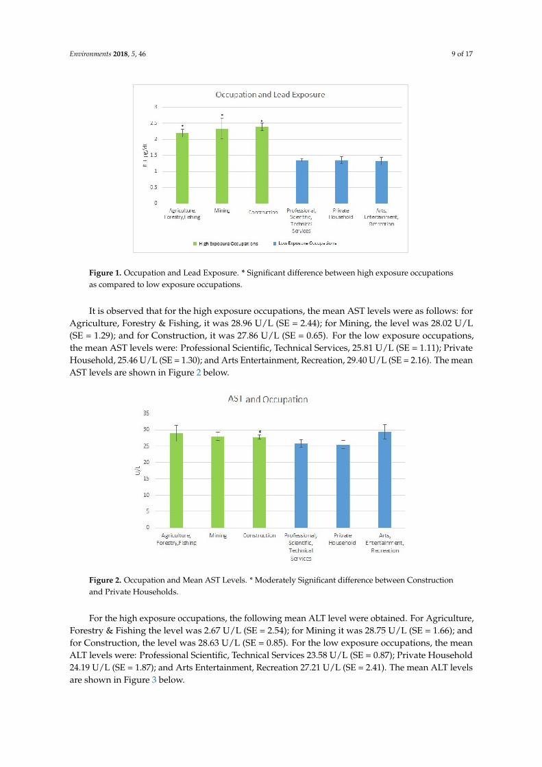
The occupations providing a high level of exposure as measured by mean BLLs were:(a) Agriculture, Forestry & Fishing 2.19 µg/dL (SE = 0.118); (b) Mining 2.33 µg/dL (SE = 0.34);and (c) Construction 2.39 µg/dL (SE = 0.12). The occupation providing the lowest levels of exposureas measured by mean BLLs were: (a) Professional, Scientific, Technical Services 1.35 µg/dL (SE = 0.05);(b) Private Household 1.35 µg/dL (SE = 0.11); and (c) Arts, Entertainment, Recreation 1.33 µg/dL(SE = 0.11). These occupations were examined to see the effects of long term exposure on makersof interest via looking at those who had these jobs as their job of longest duration. Figure 1 belowillustrates the findings.

Environments 2018, 5, 46 9 of 17

Figure 1. Occupation and Lead Exposure. * Significant difference between high exposure occupationsas compared to low exposure occupations.

It is observed that for the high exposure occupations, the mean AST levels were as follows: forAgriculture, Forestry & Fishing, it was 28.96 U/L (SE = 2.44); for Mining, the level was 28.02 U/L(SE = 1.29); and for Construction, it was 27.86 U/L (SE = 0.65). For the low exposure occupations,the mean AST levels were: Professional Scientific, Technical Services, 25.81 U/L (SE = 1.11); PrivateHousehold, 25.46 U/L (SE = 1.30); and Arts Entertainment, Recreation, 29.40 U/L (SE = 2.16). The meanAST levels are shown in Figure 2 below.

Figure 2. Occupation and Mean AST Levels. * Moderately Significant difference between Constructionand Private Households.

For the high exposure occupations, the following mean ALT level were obtained. For Agriculture,Forestry & Fishing the level was 2.67 U/L (SE = 2.54); for Mining it was 28.75 U/L (SE = 1.66); andfor Construction, the level was 28.63 U/L (SE = 0.85). For the low exposure occupations, the meanALT levels were: Professional Scientific, Technical Services 23.58 U/L (SE = 0.87); Private Household24.19 U/L (SE = 1.87); and Arts Entertainment, Recreation 27.21 U/L (SE = 2.41). The mean ALT levelsare shown in Figure 3 below.

Environments 2018, 5, 46 10 of 17

Figure 3. Occupation and Mean ALT Levels. * Moderately significant difference between Agricultureand Professional Scientific, Technical Services. # Significant difference between Mining and ProfessionalScientific, Technical Services. @ Moderately significant difference between Mining and PrivateHouseholds. + Significant difference between Construction and Professional Scientific, TechnicalServices, and Private Households.

With respect to the high exposure occupations, the following results were obtained for mean GGTlevels. For Agriculture, Forestry & Fishing the GGT level was 30.36 U/L (SE = 1.82); it was 37.41 U/L(SE = 2.25) for Mining; and 34.75 U/L (SE = 1.97) for Construction. For the low exposure occupations,the mean GGT levels were: Professional Scientific, Technical Services 24.65 U/L (SE = 2.10); PrivateHousehold 30.30 U/L (SE = 3.95); and Arts Entertainment, Recreation 27.44 U/L (SE = 3.54). The meanGGT levels are shown in Figure 4 below.

Figure 4. Occupation and Mean GGT Levels. * Significant difference between Agriculture Forestry,Fishing and Professional Scientific, Technical Services. + Significant difference between Mining andProfessional Scientific, Technical Services and Arts, Entertainment Recreation. # Significant differencebetween construction and professional.

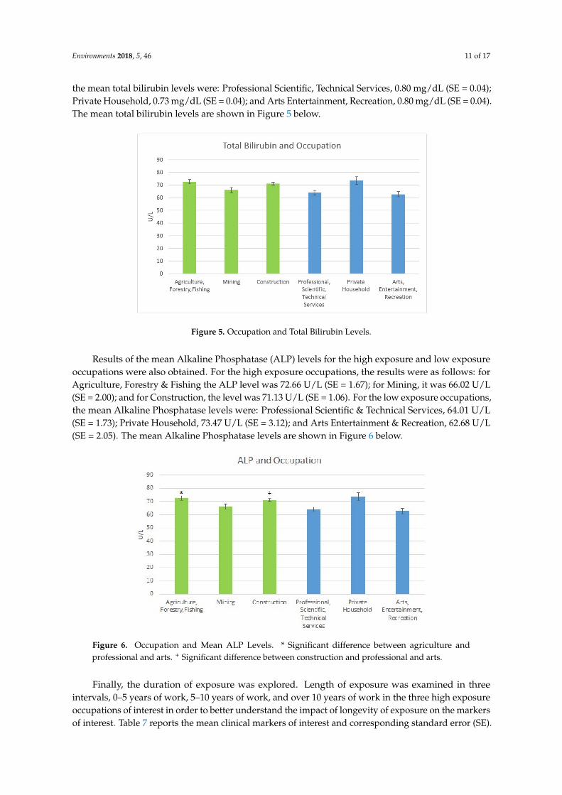
Results of the mean total bilirubin levels for the high exposure and low exposure occupations werealso obtained. For the high exposure occupations, the results were as follows: for Agriculture, Forestry& Fishing, it was 0.79 mg/dL (SE = 0.02); for Mining, the mean total bilirubin level was 0.74 mg/dL(SE = 0.03); and for Construction it was 0.79 mg/dL (SE = 0.03). For the low exposure occupations,

Environments 2018, 5, 46 11 of 17

the mean total bilirubin levels were: Professional Scientific, Technical Services, 0.80 mg/dL (SE = 0.04);Private Household, 0.73 mg/dL (SE = 0.04); and Arts Entertainment, Recreation, 0.80 mg/dL (SE = 0.04).The mean total bilirubin levels are shown in Figure 5 below.

Figure 5. Occupation and Total Bilirubin Levels.

Results of the mean Alkaline Phosphatase (ALP) levels for the high exposure and low exposureoccupations were also obtained. For the high exposure occupations, the results were as follows: forAgriculture, Forestry & Fishing the ALP level was 72.66 U/L (SE = 1.67); for Mining, it was 66.02 U/L(SE = 2.00); and for Construction, the level was 71.13 U/L (SE = 1.06). For the low exposure occupations,the mean Alkaline Phosphatase levels were: Professional Scientific & Technical Services, 64.01 U/L(SE = 1.73); Private Household, 73.47 U/L (SE = 3.12); and Arts Entertainment & Recreation, 62.68 U/L(SE = 2.05). The mean Alkaline Phosphatase levels are shown in Figure 6 below.

Figure 6. Occupation and Mean ALP Levels. * Significant difference between agriculture andprofessional and arts. + Significant difference between construction and professional and arts.

Finally, the duration of exposure was explored. Length of exposure was examined in threeintervals, 0–5 years of work, 5–10 years of work, and over 10 years of work in the three high exposureoccupations of interest in order to better understand the impact of longevity of exposure on the markersof interest. Table 7 reports the mean clinical markers of interest and corresponding standard error (SE).

Environments 2018, 5, 46 12 of 17

Table 7. Longevity in occupation and clinical markers.

TimeInterval Occupation BLL (SE) AST (SE) ALT (SE) ALP (SE) GGT (SE)

TotalBilirubin

(SE)

0–5 years Construction 1.58 (0.76) 25.54 (0.81) 26.97 (1.61) 73.62 (2.56) 28.40 (2.79) 0.86 (0.07)5–10 years Construction 2.71 (0.69) 27.72 (1.38) 30.72 (2.70) 71.10 (1.82) 35.78 (5.27) 0.71 (0.04)10+ years Construction 2.53(0.27) @, M1 28.49 (0.78) @ 28.60 (0.90) 70.49 (1.29) 36.17 (2.30) @ 0.79 (0.03) M2

0–5 years Mining 1.05 (0.43) 23.03 (2.19) 22.61 (2.60) 66.81 (3.66) 26.47 (1.42) 0.81 (0.16)5–10 years Mining 1.61 (0.28) 33.27 (4.93) M 35.62 (6.34) 66.92 (2.74) 50.77 (11.1) M1 0.71 (0.08)10+ years Mining 2.57 (0.38) +, @ 27.04 (1.57) 27.43 (2.38) 65.72 (1.98) 34.75 (3.33) 0.74 (0.03)0–5 years Agriculture 1.72 (0.38) 21.65 (0.51) 23.89 (2.40) 61.96 (4.07) 24.39 (3.52) 0.64 (0.05)5–10 years Agriculture 2.18 (0.48) 22.21 (0.90) 21.86 (2.52) 69.82 (6.15) 24.55 (3.56) 0.62 (0.06)

10+ years Agriculture 2.25 (0.12) 30.89 (3.20) @,

*30.27 (3.25)

M274.52 (1.92)

@ 31.89 (M1,2) 0.83 (0.03)@, +

@ Significantly different from 0–5 years to 10+; * Significantly different 5–10 years to 10+; + Significantly difference0–5 to 5–10; M moderately significant difference between 0–5 years and 5–10 years; M1 moderately significantdifference between 0–5 years and 10+ years; M2 moderately significant difference between 5–10 years to 10+ years.

4. Discussion

4.1. On Lead and Occupation

Cognizant of the fact that lead exposure in adults most commonly occurs in the workplace andindustries such as the construction industry, which has historically been a source of lead exposureamong adults [26], this study sough to explore occupation and its connection with lead exposure byexamining participant hepatobiliary markers in occupations. The results indicated that the quartileof exposure was related to occupation, with occupations such as mining and construction makingup a significantly larger proportion of the highest exposure quartiles (10+ µg/dL) while occupationssuch as education made up a significantly larger proportion of the lowest quartiles of exposure(0–2 µg/dL). In subsequent analysis it was determined that the occupations providing the mostexposure, as measured by BLLs in adults, were the Construction Industry; Agriculture Forestry &Fishing; and Mining. The occupations with the least exposed population were: Professional, Scientificand Technical Services; Private Household; and Arts, Entertainment and Recreation. These industrieswere examined to see how the clinical markers of interest varied between the high exposure occupationsand the lower exposure occupation.

In comparing high exposure occupations to low exposure occupations, the mean BLL’s weresignificantly higher when comparing the three high exposure occupations to the three low exposureoccupations, affirming that some occupations predispose workers to lead exposure. For example,those in Construction had significantly elevated blood pressure in the highest quartile of exposure ascompared to those in the less-exposed occupations such as Education. This is significant as it offersa means to perform targeted intervention toward higher exposure occupations. This exposure and howit manifests cannot only be tied to occupation and may also include behavioral patterns associatedwith occupations which may accelerate the negative impact of lead on the hepatic and biliary system.Some of these behaviors, including smoking and alcohol use, were adjusted for in this study in orderto offer more insight into the extent to which lead may be inducing liver damage. In addition genderand age are also potential factors altering the manifestation of these enzymes [27], hence the need toadjust for them.

For AST, a clinical marker of liver injury, there was a significant difference in the mean levelsbetween those in Construction when compared with those in Private Households, potentially indicatingthat those in a lead exposed industry experience worse outcomes than those in a less exposed industry.For ALT, there was a significant difference in the mean levels between those in the Mining occupationand those in the Professional, Scientific & Technical Services, also supporting this conclusion. There wasalso a moderately significant difference in the mean levels between those in Mining and those in PrivateHouseholds. Also, a moderately significant difference between the populations in Agriculture Forestry& Fishing compared with those in Professional Scientific and Technical services was discovered.

Environments 2018, 5, 46 13 of 17

Thus, those lead exposed industries seem to experience elevated liver injury as compared to those inless lead exposed industries.

With respect to GGT, there was a significant difference between Agriculture, Forestry & Fishingwhen compared to Professional Scientific, Technical Services. In addition, there was a significantelevation in the mean level of those in Mining when compared to those in Professional Scientific &Technical Services, and Arts, Entertainment & Recreation. Finally, there was a significant elevationin construction when compared to Professional, Scientific, and Technical Services, which confirmedthe pattern. For Alkaline Phosphatase, there was a significant elevation between Agriculture, Forestry& Fishing, and Construction when compared to Professional Scientific, Technical Services, and Arts,Entertainment, and Recreation, also confirming lead’s potential impact on the hepatic and biliary system.

Finally, in the longest held occupations, a marker of long term exposure to lead due to occupation,results for Construction demonstrated that mean BLLs were significantly elevated from the 0–5-yearworking period when compared to the 10 plus year working period, while it was moderately elevatedfrom the 0–5 to 5–10-year period. In Mining, BLLs were significantly elevated from the 0–5-year to the10+ year period and from the 0–5-year period to the 5–10-year period. Hinting at the potential adverseoutcomes over time with hepatobiliary injury becoming more severe over time.

Regarding duration of exposure, AST was moderately elevated from the 0–5 to the 5–10-yearperiod for Mining. For Construction, AST was significantly elevated from the 5–10-year to the 10+ yearperiod with Agriculture, Forestry & Fishing showing a significant elevation from 0–5 to 10+ years and5–10 to 10+ years. For ALT Agriculture, Forestry & Fishing showed a moderately significant elevationfrom 5–10 to 10+ years. For ALP, Agriculture, Forestry & Fishing showed a significant increase from0–5 to 10+ years. For GGT there was a moderately significant elevation from 0–5 to 10+ years and5–10 to 10+ years for Agriculture, Forestry & Fishing. For Mining, there was a moderately significantelevation from 0–5 to 10+ years whereas for Construction there was a significantly elevated mean from0–5 to 10+ years. Finally, for total bilirubin there was a significant elevation from 0–5 to 10+ years andfrom 0–5 to 5–10 years for Agriculture Forestry & Fishing. For Construction, there was a moderatelysignificant elevation between 5–10 years and 10+ years. This potentially indicates that exposure overa period of time may have varying effects, with some time periods being more detrimental. It must benoted that, with liver injury being multifactorial, lead may not play the largest role and other factorssuch as alcohol use, drug use, and genetic background, also contribute to liver injury [27].

4.2. On Lead and Its Role in Altering Hepatobiliary Clinical Makers

According to Lanphear and co-authors, low-level environmental lead exposure is a factor fordiseases such as cardiovascular disease [28,29]. It also seems to potentially affect the hepatic and biliarysystem. In the United States, low-level lead exposure is the norm in many communities because of thelegacy of lead exposure, which keeps populations continuously exposed. In addition, the workplaceserves as the primary avenue by which adults are exposed.

Results from this study point to the fact that participants at different binary levels of exposure havevaried presentations. For example, when lead was divided at 2 µg/dL for less-exposed/exposed, thoseexposed to lead were more likely to have high ALP (adjusted odds ratio (OR) 1.93; 95% confidenceinterval (CI) 1.42, 2.61) and GGT (adjusted OR 1.24; 95% CI 1.08, 1.42).

At the 5 µg/dL level, those exposed to lead were moderately significantly more likely to havehigher ALP (adjusted OR 2.90; 95% CI 1.18, 7.08), and GGT (adjusted OR 1.48; 95% CI 1.12, 1.95) levels.At the 10 µg/dL level those exposed to lead were more likely to have higher GGT levels (adjusted OR2.19; 95% CI 1.34, 3.56). This may indicate lead’s effects at different degrees of exposure with damagebeing manifested differently at various cutoffs.

This study found positive significant associations between BLL and ALP, GGT and total bilirubin.Regarding the exposed and less-exposed, for AST there was a significant elevation from quartile 1to quartile 2. For ALP there was a significant elevation from quartile 1 to quartile 2 and 3. Finally,for GGT there was a significant elevation from quartile 1 to quartiles 2 and 3. This speaks to increasing

Environments 2018, 5, 46 14 of 17

lead dose producing worse outcomes and that hepatobiliary clinical makers at different degrees ofexposure are potential predators of poor health outcomes and all-cause mortality as they reflect liverinjury and oxidative stress.

The effects of lead on AST and ALT have been demonstrated in the literature. Onyeneke andco-authors [24] in their study of 86 adult Nigerians who were occupationally exposed to lead and 30control subjects who were not exposed to lead (while looking to understand occupational exposure tolead in Nigeria and its relation with impairment of liver function), found that the activity of ALT andAST were significantly elevated in occupationally exposed workers as compared to controls, whereasthere was no statistically significant changes in serum total bilirubin.

Regarding GGT and its association with BLL in adults, Lee and co-authors in an analysisof NHANES III found associations between blood lead and GGT in adults [30]. Al-Neamy andco-authors [18] in their study found mean AST levels to be elevated in the exposed (31.8 ± 12.3)as compared to mean AST levels of the less-exposed (30.7 ± 13.2), however, the means were notstatistically significantly different.

For ALT, they found levels to be slightly elevated in the less-exposed (33.5 ± 24.2) as comparedto the exposed (33.2 ± 27.6) but the difference was again not statistically significant. The authorsfound the mean total bilirubin levels to be more elevated in the exposed (0.75 ± 0.3) compared to theless-exposed (0.70 ± 0.19) but these differences were not statistically significant. In addition, theyfound GGT to be elevated in the exposed (36.3 ± 35.2) as compared to the less-exposed (31.36 ± 17.9),but the difference was not statistically significant. Finally, they found ALP to be more elevated in theexposed (84.3 ± 24.6) as compared to the less-exposed (76.1 ± 20.5) with the difference proving to bestatistically significant. Thus, the results of our study, which demonstrates a statistically significantdifference in mean GGT levels between the differentially exposed individuals, contradict those ofAl-Neamy and co-authors’ study while the positive association found in regression affirms that of Leeand co-authors’ study. However, our study finding of a significant difference in the means of ALPbetween the varying degrees of exposure affirms the results of Al-Neamy and co-authors’ study.

An observation of the results of our study and those of the others show the uniqueness of ourstudy, given that it looked at larger sample sizes as compared to the non-NHANES studies. Anotherdifference is the fact that, the studies by Onyeneke [24] and Al-Neamy [18] were in Nigeria and theUAE, whereas our analysis was performed on populations in the United States.

Finally, our results regarding ALP, GGT, and total bilirubin indicate significant lead inducedpathology in the extrahepatic biliary system, potentially regarding cholestasis, as compared to theintrahepatic system, as there are significant elevations and associations in the aforementioned enzymesas compared to ALT and AST. It should be noted that even though the results regarding ALP and GGTwould strongly suggest lead induced hepatobiliary dysfunction, elevated GGT activity may occur inacute and chronic pancreatitis or even prostatic adenocarcinoma with elevated ALP also occurringin other pathology, indicating that using the absence of skeletal diseases and the absence of placentainduced elevations and pairing it with elevated ALP enzymatic activity should not be considereda clinically specific sign of hepatobiliary dysfunction [31].

4.3. Limitations of Study and Future Works

Measurement of BLLs does not indicate longer-term exposure, rather, it is indicative of recentlead exposure as well as lead that has been mobilized from bone or other tissue sources with no abilityto distinguish between both. Measuring of bone lead levels, particularly tibia lead level, via K-ShellX-Ray Fluorescence (KSXF) would have provided more information on length of exposure as bonelead levels are indicative of long-term cumulative exposure to lead. Both the BLLs and bone leadlevels taken together would have provided the best and most comprehensive view of the participant’sexposure [32]. In attempting to overcome the limitation of long-term exposure, length of time atoccupation was analyzed and seeing the differences in health outcomes overtime helped to give hintson the manifestations of long term exposure.

Environments 2018, 5, 46 15 of 17

Finally, owing to the inability to adjust for covariates in the occupational analysis, and the inabilityto perform regression analysis on lead exposed occupations due to inadequate data in all strata for anyof exposed occupations, future works should look at larger occupational databases. This will enablethe evaluation of the significances found here in adjusted models for lead exposed occupations.

5. Conclusions

Lead exposure was significantly associated with adverse hepatobiliary clinical makers, withhigher exposure resulting in worse outcomes. Looking at various degrees of exposure, lead increasedthe odds of elevated hepatobiliary clinical markers. Finally, occupational exposure may play a rolein these outcomes. These findings add to the growing body of evidence that lead exposure may bean important risk factor for liver and gallbladder dysfunction in exposed populations. Based onthe above discussion, it is suggested that a critical need exists to test novel interventions capable ofmitigating and subsequently eliminating the impact of lead on hepatobiliary health. Studies aimedat interventions that mitigate and/or eliminate the harmful effects of lead on the environment andon human health are still required for successful optimal health management. This is key as Gouldand co-authors note that every dollar invested in lead paint hazard prevention yielded $17 to $221return or a total saving of $181–$269 billion per year [33]. Finally, this study’s cross-sectional naturemeans that it portrays a snapshot in time. A longitudinal study may yield more in-depth results aspeople’s unique circumstances (finances, family, etc.) change, which may result in gaining access tonecessary knowledge and preventative measures about lead exposure and hence seeking avenues tomitigate the effects of it on their health and environment. Ultimately, this work can be used to improvepublic health by working to limit exposure to higher doses as this seems to be associated with worseliver/biliary injury but, as injury occurs at even low exposure levels it must be emphasized that nolevel of exposure is safe. Future works should look at individual, community, state, and regional-levelrisk factors of lead exposure on hepatobiliary clinical markers to better understand how these factorsmay differentially alter them and the impact at all four levels.

Acknowledgments: We acknowledge the National Center for Health Statistics of the U.S. Centers for DiseaseControl and Prevention (CDC) for its invaluable work conducting the National Health and Nutrition ExaminationSurvey, and the researchers at the Division of Laboratory Sciences, National Center for Environmental Health ofthe CDC.

Author Contributions: Emmanuel Obeng-Gyasi conceived the idea for the paper, wrote the paper, and did theanalysis. Rodrigo Armijos edited the paper and contributed to the analysis of the data. Margaret Weigel editedthe paper and provided analytical evaluation. Gabriel Filippelli provided analytical guidance for the paper.M. Aaron Sayegh provided analytical guidance for the paper.

Conflicts of Interest: The authors declare no conflict of interest.

References

1. Centers for Disease Control and Prevention. Very high blood lead levels among adults-United States, 2002–2011.MMWR. Morb. Mort. Wkly Rep. 2013, 62, 967–971.

2. Jarup, L. Hazards of heavy metal contamination. Br. Med. Bull. 2003, 68, 167–182. [CrossRef] [PubMed]3. Mielke, H.W.; Laidlaw, M.A.; Gonzales, C. Lead (Pb) legacy from vehicle traffic in eight California urbanized

areas: Continuing influence of lead dust on children’s health. Sci. Total Environ. 2010, 408, 3965–3975.[CrossRef] [PubMed]

4. Johnson, S.; Saikia, N.; Sahu, M.R. Lead in Paints; Centre for Science and Environment, and PollutionMonitoring Laboratory: New Delhi, India, 2009.

5. Díaz-Barriga, F.; Batres, L.; Calderón, J.; Lugo, A.; Galvao, L.; Lara, I.; Rizo, P.; Arroyave, M.E.; McConnell, R.The El Paso smelter 20 years later: Residual impact on Mexican children. Environ. Res. 1997, 74, 11–16.[CrossRef] [PubMed]

6. Oldereid, N.B.; Thomassen, Y.; Attramadal, A.; Olaisen, B.; Purvis, K. Concentrations of lead, cadmium andzinc in the tissues of reproductive organs of men. J. Reprod. Fertil. 1993, 99, 421–425. [CrossRef] [PubMed]

Environments 2018, 5, 46 16 of 17

7. Navas-Acien, A.; Guallar, E.; Silbergeld, E.K.; Rothenberg, S.J. Lead exposure and cardiovascular disease:A systematic review. Environ. Health Perspect. 2007, 115, 472–482. [CrossRef] [PubMed]

8. Dioka, C.E.; Orisakwe, O.E.; Adeniyi, F.A.A.; Meludu, S.C. Liver and renal function tests in artisansoccupationally exposed to lead in mechanic village in Nnewi, Nigeria. Int. J. Environ. Res. Public Health 2004,1, 21–25. [CrossRef] [PubMed]

9. Bellinger, D.; Leviton, A.; Waternaux, C.; Needleman, H.; Rabinowitz, M. Longitudinal analyses of prenataland postnatal lead exposure and early cognitive development. N. Engl. J. Med. 1987, 316, 1037–1043.[CrossRef] [PubMed]

10. Darwish, W.S.; Ikenaka, Y. Biological responses of xenobiotic metabolizing enzymes to lead exposure incultured H4IIE rat cells. Jpn. J. Vet. Res. 2013, 61, S48–S53. [PubMed]

11. Hsu, P.-C.; Guo, Y.L. Antioxidant nutrients and lead toxicity. Toxicology 2002, 180, 33–44. [CrossRef]12. Kim, Y.J. Interpretation of liver function tests. Korean J. Gastroenterol. Taehan Sohwagi Hakhoe chi 2008, 51,

219–224. [PubMed]13. Centers for Disease Control and Prevention. Summary Health Statistics Tables for US Adults: National

Health Interview Survey 2015, Table A-4b. Available online: https://ftp.cdc.gov/pub/Health_Statistics/NCHS/NHIS/SHS/2015_SHS_Table_A-4.pdf (accessed on 1 April 2017).

14. Green, R.M.; Flamm, S. AGA technical review on the evaluation of liver chemistry tests. Gastroenterology2002, 123, 1367–1384. [CrossRef] [PubMed]

15. Johnston, D.E. Special considerations in interpreting liver function tests. Am. Fam. Physician 1999, 59,2223–2232. [PubMed]

16. Washington, I.M.; Van Hoosier, G. Clinical biochemistry and hematology. In The Laboratory Rabbit, GuineaPig, Hamster, and Other Rodents; Elsevier: Amsterdam, The Netherlands, 2012; pp. 57–116.

17. Giannini, E.G.; Testa, R.; Savarino, V. Liver enzyme alteration: A guide for clinicians. Can. Med. Assoc. J.2005, 172, 367–379. [CrossRef] [PubMed]

18. Al-Neamy, F.R.M.; Almehdi, A.M.; Alwash, R.; Pasha, M.A.H.; Ibrahim, A.; Bener, A. Occupational leadexposure and amino acid profiles and liver function tests in industrial workers. Int. J. Environ. Health Res.2001, 11, 181–188. [CrossRef] [PubMed]

19. Papanikolaou, N.C.; Hatzidaki, E.G.; Belivanis, S.; Tzanakakis, G.N.; Tsatsakis, A.M. Lead toxicity update.A brief review. Med. Sci. Monit. 2005, 11, RA329–RA336. [PubMed]

20. National Center for Health Statistics (NCHS). National Health and Nutrition Examination SurveyQuestionnaire (or examination protocol, or laboratory protocol). 2008. Available online: https://wwwn.cdc.gov/nchs/nhanes/ContinuousNhanes/Default.aspx?BeginYear=2007 (accessed on 31 March 2018).

21. National Center for Health Statistics (NCHS). National Health and Nutrition Examination SurveyQuestionnaire (or examination protocol, or laboratory protocol). 2010. Available online: https://wwwn.cdc.gov/nchs/nhanes/ContinuousNhanes/Default.aspx?BeginYear=2009 (accessed on 31 March 2018).

22. Sakai, T. Biomarkers of lead exposure. Ind. Health 2000, 38, 127–142. [CrossRef] [PubMed]23. Geraldine, M.; Venkatesh, T. Influence of minerals on lead-induced alterations in liver function in rats

exposed to long-term lead exposure. J. Hazard. Mater. 2009, 166, 1410–1414.24. Onyeneke, E.C.; Omokaro, E.U. Effect of Occupational Exposure to Lead on Liver Function Parameters. Int. J.

Pharm. Med. Sci. 2016, 6, 15–19.25. National Center for Health Statistics. National Health and Nutrition Examination Survey (NHANES) Analytic

Guidelines; US Department of Health and Human Services: Washington, DC, USA, 2007.26. Waller, K.; Osorio, A.M.; Maizlish, N.; Royce, S. Lead exposure in the construction industry: Results from

the California Occupational Lead Registry, 1987 through 1989. Am. J. Public Health 1992, 82, 1669–1671.[CrossRef] [PubMed]

27. Van Beek, J.H.; de Moor, M.H.; de Geus, E.J.; Lubke, G.H.; Vink, J.M.; Willemsen, G.; Boomsma, D.I.The genetic architecture of liver enzyme levels: GGT, ALT and AST. Behav. Genet. 2013, 43, 329–339.[CrossRef] [PubMed]

28. Lanphear, B.P.; Hornung, R.; Khoury, J.; Yolton, K.; Baghurst, P.; Bellinger, D.C.; Canfield, R.L.; Dietrich, K.N.;Bornschein, R.; Greene, T.; et al. Low-level environmental lead exposure and children’s intellectual function:An international pooled analysis. Environ. Health Perspect. 2005, 113, 894–899. [CrossRef] [PubMed]

29. Lanphear, B.P.; Rauch, S.; Auinger, P.; Allen, R.W.; Hornung, R.W. Low-level lead exposure and mortality inUS adults: A population-based cohort study. Lancet Public Health 2018. [CrossRef]

Environments 2018, 5, 46 17 of 17

30. Lee, D.H.; Lim, J.S.; Song, K.; Boo, Y.; Jacobs, D.R., Jr. Graded associations of blood lead and urinary cadmiumconcentrations with oxidative-stress–related markers in the US population: Results from the Third NationalHealth and Nutrition Examination Survey. Environ. Health Perspect. 2006, 114, 350–354. [CrossRef] [PubMed]

31. Clark, V.L.; Kruse, J.A. Clinical methods: The history, physical, and laboratory examinations. JAMA 1990,264, 2808–2809.

32. Landrigan, P.J.; Todd, A.C. Direct measurement of lead in bone a promising biomarker. JAMA 1994, 271,239–240. [CrossRef] [PubMed]

33. Gould, E. Childhood lead poisoning: Conservative estimates of the social and economic benefits of leadhazard control. Environ. Health Perspect. 2009, 117, 1162–1167. [CrossRef] [PubMed]

© 2018 by the authors. Licensee MDPI, Basel, Switzerland. This article is an open accessarticle distributed under the terms and conditions of the Creative Commons Attribution(CC BY) license (http://creativecommons.org/licenses/by/4.0/).