High Speed Camera & IMUs on Mobile Devices

Instructor - Simon Lucey

16-623 - Designing Computer Vision Apps

Today

• CCD vs CMOS cameras.

• Rolling Shutter Epipolar Geometry

• Inertial Measurement Units (IMU)

Pinhole Camera

3

2 SERGE BELONGIE, CSE 252B: COMPUTER VISION II

Figure 1. The pinhole imaging model, from Forsyth & Ponce.

Let us begin by considering a mathematical description of the imagingprocess through this idealized camera. We will consider issues like lens dis-tortion subsequently.

The pinhole camera or the projective camera as it is known images thescene by applying a perspective projection to it. In the following we shall re-fer to scene coordinates with upper case roman letters, {X, Y, Z, . . .}. Imagecoordinates will be referred to using lower case roman letters, {x, y, z, . . .}.Vectors shall be denoted by boldfaced symbols, e.g., X or x. (In class, whenwriting on the blackboard, I will put a tilde underneath the correspondingsymbols to denote a vector.)

The scene is three dimensional, whereas the image is located in a twodimensional plane. Hence the perspective projection maps the 3D space toa 2D plane.

(X, Y, Z)>Projection������! (x, y)>

The equations of perspective projections are given by

(1.1) x = fX

Zy = f

Y

Zhere, f is the focal length of the camera, i.e., the distance between the imageplane and the pinhole.

The process is illustrated in figure 2.

C

Y

y

Y

x

X

x

p

image plane

camera

centre

Z

principal axis

C

X

Figure 2. Image formation in a projective camera.

(Taken from Forsyth & Ponce)

Pinhole Camera

3

2 SERGE BELONGIE, CSE 252B: COMPUTER VISION II

Figure 1. The pinhole imaging model, from Forsyth & Ponce.

Let us begin by considering a mathematical description of the imagingprocess through this idealized camera. We will consider issues like lens dis-tortion subsequently.

The pinhole camera or the projective camera as it is known images thescene by applying a perspective projection to it. In the following we shall re-fer to scene coordinates with upper case roman letters, {X, Y, Z, . . .}. Imagecoordinates will be referred to using lower case roman letters, {x, y, z, . . .}.Vectors shall be denoted by boldfaced symbols, e.g., X or x. (In class, whenwriting on the blackboard, I will put a tilde underneath the correspondingsymbols to denote a vector.)

The scene is three dimensional, whereas the image is located in a twodimensional plane. Hence the perspective projection maps the 3D space toa 2D plane.

(X, Y, Z)>Projection������! (x, y)>

The equations of perspective projections are given by

(1.1) x = fX

Zy = f

Y

Zhere, f is the focal length of the camera, i.e., the distance between the imageplane and the pinhole.

The process is illustrated in figure 2.

C

Y

y

Y

x

X

x

p

image plane

camera

centre

Z

principal axis

C

X

Figure 2. Image formation in a projective camera.

(Taken from Forsyth & Ponce)

imaging sensor

Digital Cameras

• All digital cameras rely on the photoelectric effect to create electrical signal from light.

• CCD (charge coupled device) and CMOS (complementary metal oxide semiconductor) are the two most common image sensors found in digital cameras.

• Both invented in the late 60s early 70s.

(Taken from https://www.teledynedalsa.com/imaging/knowledge-center/appnotes/ccd-vs-cmos/)

CCD versus CMOS

• CMOS and CCD imagers differ in the way that signals are converted from signal charge.

• CMOS imagers are inherently more parallel than CCDs.

• Consequently, high speed CMOS imagers can be designed to have much lower noise than high speed CCDs.

(Taken from https://www.teledynedalsa.com/imaging/knowledge-center/appnotes/ccd-vs-cmos/)

CCD versus CMOS

• CCD used to be the image sensor of choice as it gave far superior images with the fabrication technology available.

• CMOS was of interest with the the advent of mobile phones. • CMOS promised lower power consumption. • lowered fabrication costs (reuse mainstream logic and memory device

fabrication).

• An enormous amount of investment was made to develop and fine tune CMOS imagers.

• As a result we witnessed great improvements in image quality, even as pixel sizes shrank.

• In the case of high volume consumer area imagers, CMOS imagers outperform CCDs based on almost every performance parameter.

(Taken from https://www.teledynedalsa.com/imaging/knowledge-center/appnotes/ccd-vs-cmos/)

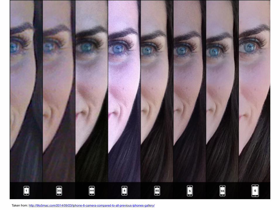
Taken from: http://9to5mac.com/2014/09/23/iphone-6-camera-compared-to-all-previous-iphones-gallery/

New Developments - iPhone 7

9Taken from: http://vrscout.com/news/apple-duel-camera-iphone-for-augmented-reality/

• Apple just released the iPhone 7 with new dual lens camera. • Rumored that advances in the camera are based on the 2015

acquisition of Linx (Israeli startup). • Image quality “closest” attempt yet to DSLR on mobile device.

Today

• CCD vs CMOS cameras.

• Rolling Shutter Epipolar Geometry

• Inertial Measurement Units (IMU)

Rolling Shutter Effect

11

from inertial measurement sensors. The readings of accelerom-eters capture not only linear acceleration of cameras, butalso gravity and acceleration caused by rotation. Besides,acceleration readings must be integrated twice to obtain thecamera translation, which makes the estimation more proneto measurement noise. Even if we can obtain accurate cameratranslation, the video rectification and stabilization problem isstill ill-posed since it is impossible to obtain depth informationfor every image pixel. Dense warping [3] and image-based ren-dering [7] have been applied to approximate the stabilizationresults based on sparse 3-D scene reconstruction. However,they are computationally prohibitive for many handheld plat-forms.Fortunately, camera shake and rolling shutter effects are

caused primarily by camera rotations. In fact, [4] and [8]have shown that taking only camera rotations into account issufficient to produce satisfactory videos.In our paper, we also use gyroscope readings. In the

gyroscope-only method [4] the camera rotation is directlyestimated by integrating the gyroscope readings (angular ve-locities). Another recent approach [5] uses both gyroscopeand accelerometer readings to estimate the camera rotationsbased on EKF. The gyroscope readings are used as the controlinputs in the dynamic motion model. The authors assume thatusers usually try to hold the camera in a steady position so thegravity is approximately the only source in the accelerometermeasurements. Thus the accelerometer readings can be usedas measurements of the camera rotation.Our 3-D orientation estimation is also based on EKF, but

our measurement model is quite different from [5]. We findthat the linear acceleration of the camera and the accelerationcaused by rotation are sometimes non-negligible. Thus we donot use the accelerometer readings as orientation measure-ments. Instead, we use the tracked feature points extractedfrom the video frames, which provide accurate geometric cluefor the estimation of the camera motion. Based on the factthat matched feature points can be related by a homographictransformation under pure rotational motion, the relative rota-tion between consecutive frames can be measured [9].Motion estimation based on visual and inertial measurement

sensors have been extensively studied in the problem ofsimultaneous localization and mapping (SLAM) in robotics[10]. However, the rolling shutter camera model has never beenconsidered in SLAM before. Our algorithm is the first EKF-based motion estimation method for rolling-shutter camerasthat uses visual and inertial measurements. In our measure-ment model, tracked feature points in consecutive frames areonly linked by the relative camera rotation between them.Therefore, our algorithm can be classified as a relative motionestimation method [11], [12].

III. CAMERA MODEL

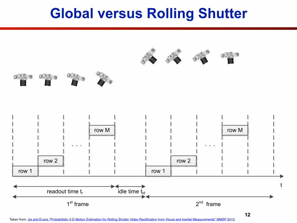
For rolling shutter cameras, each row in a frame is exposedat a different time. Fig. 2 illustrates the image capture modelof a rolling shutter camera, where tr is the total readout timein each frame and tid is the inter-frame idle time. Thus for

Fig. 2. Rolling shutter cameras sequentially expose rows. tr + tid =1

frame per second .

an image point u = [u0, u1]T in frame i, the exposure time ist(u, i) = ti + tr ×

u1

h, where ti is the timestamp of frame i

and h is the total number of rows in each frame.Assume the intrinsic camera matrix is K, the sequences

of rotation matrices and translation vectors of the camera areR(t) and l(t). A 3-D point x and its projection image u inframe i should satisfy the following equation:

u ∼ KR(t(u, i))(x + l(t(u, i))) (1)

where ∼ indicates equality up to scale.Usually there is a constant delay td between the recorded

timestamps of gyroscopes and videos. Thus using the times-tamps of gyroscopes as reference, the exposure time equationshould be modified as

t(u, i) = ti + td + tr ×uy

h. (2)

When pure rotation is considered, the translation vectorremains unchanged and thus the image of a certain scene pointin one frame can be mapped to another frame through a 3× 3homography matrix

u′ ∼ KR(t(u′, i))RT (t(u, j))K−1u (3)

where u′ and u are the images in frame i and j respectively.

IV. ONLINE ROTATION ESTIMATIONOur online motion estimation is based on EKF. Due to

the special property of rolling shutter camera model and thepure rotation motion model, state definition and the structureof dynamical and measurement model need to be designedcarefully.

A. State Vector and Dynamic Bayesian NetworkThe gyroscope in cell phone cameras usually has a higher

sampling frequency (around 100 Hz) than the video frame rate,as illustrated in Fig. 3.In Fig. 3, several gyroscope readings are grouped together

since they are used to compute the camera rotations for thesame frame during its corresponding exposure time. Note thatdue to the fact that the idle time tid is large enough so thatno pixels in frame i but only several pixels in frame i+1 areexposed after τk+3. Thus ωk+3 is relegated to group i + 1.Further we assume that a certain 3-D feature point has itsprojection at u in frame i and u′ in frame i + 1. Without

Rolling shutter cameras sequentially expose rows.

Taken from: Jia and Evans “Probabilistic 3-D Motion Estimation for Rolling Shutter Video Rectification from Visual and Inertial Measurements” MMSP 2012.

tr + tid =

1

frames per second

Global versus Rolling Shutter

12

from inertial measurement sensors. The readings of accelerom-eters capture not only linear acceleration of cameras, butalso gravity and acceleration caused by rotation. Besides,acceleration readings must be integrated twice to obtain thecamera translation, which makes the estimation more proneto measurement noise. Even if we can obtain accurate cameratranslation, the video rectification and stabilization problem isstill ill-posed since it is impossible to obtain depth informationfor every image pixel. Dense warping [3] and image-based ren-dering [7] have been applied to approximate the stabilizationresults based on sparse 3-D scene reconstruction. However,they are computationally prohibitive for many handheld plat-forms.Fortunately, camera shake and rolling shutter effects are

caused primarily by camera rotations. In fact, [4] and [8]have shown that taking only camera rotations into account issufficient to produce satisfactory videos.In our paper, we also use gyroscope readings. In the

gyroscope-only method [4] the camera rotation is directlyestimated by integrating the gyroscope readings (angular ve-locities). Another recent approach [5] uses both gyroscopeand accelerometer readings to estimate the camera rotationsbased on EKF. The gyroscope readings are used as the controlinputs in the dynamic motion model. The authors assume thatusers usually try to hold the camera in a steady position so thegravity is approximately the only source in the accelerometermeasurements. Thus the accelerometer readings can be usedas measurements of the camera rotation.Our 3-D orientation estimation is also based on EKF, but

our measurement model is quite different from [5]. We findthat the linear acceleration of the camera and the accelerationcaused by rotation are sometimes non-negligible. Thus we donot use the accelerometer readings as orientation measure-ments. Instead, we use the tracked feature points extractedfrom the video frames, which provide accurate geometric cluefor the estimation of the camera motion. Based on the factthat matched feature points can be related by a homographictransformation under pure rotational motion, the relative rota-tion between consecutive frames can be measured [9].Motion estimation based on visual and inertial measurement

sensors have been extensively studied in the problem ofsimultaneous localization and mapping (SLAM) in robotics[10]. However, the rolling shutter camera model has never beenconsidered in SLAM before. Our algorithm is the first EKF-based motion estimation method for rolling-shutter camerasthat uses visual and inertial measurements. In our measure-ment model, tracked feature points in consecutive frames areonly linked by the relative camera rotation between them.Therefore, our algorithm can be classified as a relative motionestimation method [11], [12].

III. CAMERA MODEL

For rolling shutter cameras, each row in a frame is exposedat a different time. Fig. 2 illustrates the image capture modelof a rolling shutter camera, where tr is the total readout timein each frame and tid is the inter-frame idle time. Thus for

Fig. 2. Rolling shutter cameras sequentially expose rows. tr + tid =1

frame per second .

an image point u = [u0, u1]T in frame i, the exposure time ist(u, i) = ti + tr ×

u1

h, where ti is the timestamp of frame i

and h is the total number of rows in each frame.Assume the intrinsic camera matrix is K, the sequences

of rotation matrices and translation vectors of the camera areR(t) and l(t). A 3-D point x and its projection image u inframe i should satisfy the following equation:

u ∼ KR(t(u, i))(x + l(t(u, i))) (1)

where ∼ indicates equality up to scale.Usually there is a constant delay td between the recorded

timestamps of gyroscopes and videos. Thus using the times-tamps of gyroscopes as reference, the exposure time equationshould be modified as

t(u, i) = ti + td + tr ×uy

h. (2)

When pure rotation is considered, the translation vectorremains unchanged and thus the image of a certain scene pointin one frame can be mapped to another frame through a 3× 3homography matrix

u′ ∼ KR(t(u′, i))RT (t(u, j))K−1u (3)

where u′ and u are the images in frame i and j respectively.

IV. ONLINE ROTATION ESTIMATIONOur online motion estimation is based on EKF. Due to

the special property of rolling shutter camera model and thepure rotation motion model, state definition and the structureof dynamical and measurement model need to be designedcarefully.

A. State Vector and Dynamic Bayesian NetworkThe gyroscope in cell phone cameras usually has a higher

sampling frequency (around 100 Hz) than the video frame rate,as illustrated in Fig. 3.In Fig. 3, several gyroscope readings are grouped together

since they are used to compute the camera rotations for thesame frame during its corresponding exposure time. Note thatdue to the fact that the idle time tid is large enough so thatno pixels in frame i but only several pixels in frame i+1 areexposed after τk+3. Thus ωk+3 is relegated to group i + 1.Further we assume that a certain 3-D feature point has itsprojection at u in frame i and u′ in frame i + 1. Without

Taken from: Jia and Evans “Probabilistic 3-D Motion Estimation for Rolling Shutter Video Rectification from Visual and Inertial Measurements” MMSP 2012.

Stru

ctur

e an

d M

otio

n

Rec

onst

ruct

•S

cene

geo

met

ry•C

amer

a m

otio

n

Unk

now

nca

mer

avi

ewpo

ints

Stru

ctur

e an

d M

otio

n fro

m D

iscr

ete

Vie

ws

•In

trodu

ctio

n

•C

ompu

ting

the

fund

amen

tal m

atrix

, F, f

rom

cor

ner c

orre

spon

denc

es

•Fe

atur

e m

atch

ing

•R

AN

SA

C

•E

stim

atio

n

•D

eter

min

ing

ego-

mot

ion

from

F

•S

IFT

for w

ide

base

line

mat

chin

g

•C

ompu

ting

a ho

mog

raph

y, H

, fro

m c

orne

r cor

resp

onde

nces

•M

ore

than

two

view

s

•B

atch

and

seq

uent

ial s

olut

ions

Stru

ctur

e an

d M

otio

n

Rec

onst

ruct

•S

cene

geo

met

ry•C

amer

a m

otio

n

Unk

now

nca

mer

avi

ewpo

ints

Stru

ctur

e an

d M

otio

n fro

m D

iscr

ete

Vie

ws

•In

trodu

ctio

n

•C

ompu

ting

the

fund

amen

tal m

atrix

, F, f

rom

cor

ner c

orre

spon

denc

es

•Fe

atur

e m

atch

ing

•R

AN

SA

C

•E

stim

atio

n

•D

eter

min

ing

ego-

mot

ion

from

F

•S

IFT

for w

ide

base

line

mat

chin

g

•C

ompu

ting

a ho

mog

raph

y, H

, fro

m c

orne

r cor

resp

onde

nces

•M

ore

than

two

view

s

•B

atch

and

seq

uent

ial s

olut

ions

Stru

ctur

e an

d M

otio

n

Rec

onst

ruct

•S

cene

geo

met

ry•C

amer

a m

otio

n

Unk

now

nca

mer

avi

ewpo

ints

Stru

ctur

e an

d M

otio

n fro

m D

iscr

ete

Vie

ws

•In

trodu

ctio

n

•C

ompu

ting

the

fund

amen

tal m

atrix

, F, f

rom

cor

ner c

orre

spon

denc

es

•Fe

atur

e m

atch

ing

•R

AN

SA

C

•E

stim

atio

n

•D

eter

min

ing

ego-

mot

ion

from

F

•S

IFT

for w

ide

base

line

mat

chin

g

•C

ompu

ting

a ho

mog

raph

y, H

, fro

m c

orne

r cor

resp

onde

nces

•M

ore

than

two

view

s

•B

atch

and

seq

uent

ial s

olut

ions

Stru

ctur

e an

d M

otio

n

Rec

onst

ruct

•S

cene

geo

met

ry•C

amer

a m

otio

n

Unk

now

nca

mer

avi

ewpo

ints

Stru

ctur

e an

d M

otio

n fro

m D

iscr

ete

Vie

ws

•In

trodu

ctio

n

•C

ompu

ting

the

fund

amen

tal m

atrix

, F, f

rom

cor

ner c

orre

spon

denc

es

•Fe

atur

e m

atch

ing

•R

AN

SA

C

•E

stim

atio

n

•D

eter

min

ing

ego-

mot

ion

from

F

•S

IFT

for w

ide

base

line

mat

chin

g

•C

ompu

ting

a ho

mog

raph

y, H

, fro

m c

orne

r cor

resp

onde

nces

•M

ore

than

two

view

s

•B

atch

and

seq

uent

ial s

olut

ions

Structu

re and Motio

nReco

nstruct

•Scene geometry

•Camera motio

n

Unknown

camera

viewpoints

Structu

re and Motio

n from Disc

rete Views

•Intro

duction

•Computin

g the fu

ndamental matrix

, F, fr

om corner c

orresp

ondences

•Feature m

atching

•RANSAC

•Esti

mation

•Determ

ining ego-motio

n from F

•SIFT fo

r wide base

line match

ing

•Computin

g a homography, H, fr

om corner c

orresp

ondences

•More th

an two vie

ws

•Batch

and sequentia

l solutio

ns

Structu

re and Motio

nReco

nstruct

•Scene geometry

•Camera motio

n

Unknown

camera

viewpoints

Structu

re and Motio

n from Disc

rete Views

•Intro

duction

•Computin

g the fu

ndamental matrix

, F, fr

om corner c

orresp

ondences

•Feature m

atching

•RANSAC

•Esti

mation

•Determ

ining ego-motio

n from F

•SIFT fo

r wide base

line match

ing

•Computin

g a homography, H, fr

om corner c

orresp

ondences

•More th

an two vie

ws

•Batch

and sequentia

l solutio

ns

Structu

re and Motio

nReco

nstruct

•Scene geometry

•Camera motio

n

Unknown

camera

viewpoints

Structu

re and Motio

n from Disc

rete Views

•Intro

duction

•Computin

g the fu

ndamental matrix

, F, fr

om corner c

orresp

ondences

•Feature m

atching

•RANSAC

•Esti

mation

•Determ

ining ego-motio

n from F

•SIFT fo

r wide base

line match

ing

•Computin

g a homography, H, fr

om corner c

orresp

ondences

•More th

an two vie

ws

•Batch

and sequentia

l solutio

ns

Structu

re and Motio

nReco

nstruct

•Scene geometry

•Camera motio

n

Unknown

camera

viewpoints

Structu

re and Motio

n from Disc

rete Views

•Intro

duction

•Computin

g the fu

ndamental matrix

, F, fr

om corner c

orresp

ondences

•Feature m

atching

•RANSAC

•Esti

mation

•Determ

ining ego-motio

n from F

•SIFT fo

r wide base

line match

ing

•Computin

g a homography, H, fr

om corner c

orresp

ondences

•More th

an two vie

ws

•Batch

and sequentia

l solutio

ns

Global versus Rolling Shutter

12

from inertial measurement sensors. The readings of accelerom-eters capture not only linear acceleration of cameras, butalso gravity and acceleration caused by rotation. Besides,acceleration readings must be integrated twice to obtain thecamera translation, which makes the estimation more proneto measurement noise. Even if we can obtain accurate cameratranslation, the video rectification and stabilization problem isstill ill-posed since it is impossible to obtain depth informationfor every image pixel. Dense warping [3] and image-based ren-dering [7] have been applied to approximate the stabilizationresults based on sparse 3-D scene reconstruction. However,they are computationally prohibitive for many handheld plat-forms.Fortunately, camera shake and rolling shutter effects are

caused primarily by camera rotations. In fact, [4] and [8]have shown that taking only camera rotations into account issufficient to produce satisfactory videos.In our paper, we also use gyroscope readings. In the

gyroscope-only method [4] the camera rotation is directlyestimated by integrating the gyroscope readings (angular ve-locities). Another recent approach [5] uses both gyroscopeand accelerometer readings to estimate the camera rotationsbased on EKF. The gyroscope readings are used as the controlinputs in the dynamic motion model. The authors assume thatusers usually try to hold the camera in a steady position so thegravity is approximately the only source in the accelerometermeasurements. Thus the accelerometer readings can be usedas measurements of the camera rotation.Our 3-D orientation estimation is also based on EKF, but

our measurement model is quite different from [5]. We findthat the linear acceleration of the camera and the accelerationcaused by rotation are sometimes non-negligible. Thus we donot use the accelerometer readings as orientation measure-ments. Instead, we use the tracked feature points extractedfrom the video frames, which provide accurate geometric cluefor the estimation of the camera motion. Based on the factthat matched feature points can be related by a homographictransformation under pure rotational motion, the relative rota-tion between consecutive frames can be measured [9].Motion estimation based on visual and inertial measurement

sensors have been extensively studied in the problem ofsimultaneous localization and mapping (SLAM) in robotics[10]. However, the rolling shutter camera model has never beenconsidered in SLAM before. Our algorithm is the first EKF-based motion estimation method for rolling-shutter camerasthat uses visual and inertial measurements. In our measure-ment model, tracked feature points in consecutive frames areonly linked by the relative camera rotation between them.Therefore, our algorithm can be classified as a relative motionestimation method [11], [12].

III. CAMERA MODEL

For rolling shutter cameras, each row in a frame is exposedat a different time. Fig. 2 illustrates the image capture modelof a rolling shutter camera, where tr is the total readout timein each frame and tid is the inter-frame idle time. Thus for

Fig. 2. Rolling shutter cameras sequentially expose rows. tr + tid =1

frame per second .

an image point u = [u0, u1]T in frame i, the exposure time ist(u, i) = ti + tr ×

u1

h, where ti is the timestamp of frame i

and h is the total number of rows in each frame.Assume the intrinsic camera matrix is K, the sequences

of rotation matrices and translation vectors of the camera areR(t) and l(t). A 3-D point x and its projection image u inframe i should satisfy the following equation:

u ∼ KR(t(u, i))(x + l(t(u, i))) (1)

where ∼ indicates equality up to scale.Usually there is a constant delay td between the recorded

timestamps of gyroscopes and videos. Thus using the times-tamps of gyroscopes as reference, the exposure time equationshould be modified as

t(u, i) = ti + td + tr ×uy

h. (2)

When pure rotation is considered, the translation vectorremains unchanged and thus the image of a certain scene pointin one frame can be mapped to another frame through a 3× 3homography matrix

u′ ∼ KR(t(u′, i))RT (t(u, j))K−1u (3)

where u′ and u are the images in frame i and j respectively.

IV. ONLINE ROTATION ESTIMATIONOur online motion estimation is based on EKF. Due to

the special property of rolling shutter camera model and thepure rotation motion model, state definition and the structureof dynamical and measurement model need to be designedcarefully.

A. State Vector and Dynamic Bayesian NetworkThe gyroscope in cell phone cameras usually has a higher

sampling frequency (around 100 Hz) than the video frame rate,as illustrated in Fig. 3.In Fig. 3, several gyroscope readings are grouped together

since they are used to compute the camera rotations for thesame frame during its corresponding exposure time. Note thatdue to the fact that the idle time tid is large enough so thatno pixels in frame i but only several pixels in frame i+1 areexposed after τk+3. Thus ωk+3 is relegated to group i + 1.Further we assume that a certain 3-D feature point has itsprojection at u in frame i and u′ in frame i + 1. Without

Taken from: Jia and Evans “Probabilistic 3-D Motion Estimation for Rolling Shutter Video Rectification from Visual and Inertial Measurements” MMSP 2012.

Stru

ctur

e an

d M

otio

n

Rec

onst

ruct

•S

cene

geo

met

ry•C

amer

a m

otio

n

Unk

now

nca

mer

avi

ewpo

ints

Stru

ctur

e an

d M

otio

n fro

m D

iscr

ete

Vie

ws

•In

trodu

ctio

n

•C

ompu

ting

the

fund

amen

tal m

atrix

, F, f

rom

cor

ner c

orre

spon

denc

es

•Fe

atur

e m

atch

ing

•R

AN

SA

C

•E

stim

atio

n

•D

eter

min

ing

ego-

mot

ion

from

F

•S

IFT

for w

ide

base

line

mat

chin

g

•C

ompu

ting

a ho

mog

raph

y, H

, fro

m c

orne

r cor

resp

onde

nces

•M

ore

than

two

view

s

•B

atch

and

seq

uent

ial s

olut

ions

Stru

ctur

e an

d M

otio

n

Rec

onst

ruct

• S

cene

geo

met

ry• C

amer

a m

otio

n

Unk

now

nca

mer

avi

ewpo

ints

Stru

ctur

e an

d M

otio

n fro

m D

iscr

ete

Vie

ws

•In

trodu

ctio

n•

Com

putin

g th

e fu

ndam

enta

l mat

rix, F

, fro

m c

orne

r cor

resp

onde

nces

•Fe

atur

e m

atch

ing

•R

AN

SA

C•

Est

imat

ion

•D

eter

min

ing

ego-

mot

ion

from

F•

SIF

T fo

r wid

e ba

selin

e m

atch

ing

•C

ompu

ting

a ho

mog

raph

y, H

, fro

m c

orne

r cor

resp

onde

nces

•M

ore

than

two

view

s•

Bat

ch a

nd s

eque

ntia

l sol

utio

ns

Stru

ctur

e an

d M

otio

n

Rec

onst

ruct

• S

cene

geo

met

ry• C

amer

a m

otio

n

Unk

now

nca

mer

avi

ewpo

ints

Stru

ctur

e an

d M

otio

n fro

m D

iscr

ete

Vie

ws

•In

trodu

ctio

n•

Com

putin

g th

e fu

ndam

enta

l mat

rix, F

, fro

m c

orne

r cor

resp

onde

nces

•Fe

atur

e m

atch

ing

•R

AN

SA

C•

Est

imat

ion

•D

eter

min

ing

ego-

mot

ion

from

F

•S

IFT

for w

ide

base

line

mat

chin

g

•C

ompu

ting

a ho

mog

raph

y, H

, fro

m c

orne

r cor

resp

onde

nces

•M

ore

than

two

view

s•

Bat

ch a

nd s

eque

ntia

l sol

utio

ns

Stru

ctur

e an

d M

otio

nRe

cons

truct

• S

cene

geo

met

ry

• Cam

era

mot

ion

Unkn

own

cam

era

viewp

oint

s

Stru

ctur

e an

d M

otio

n fro

m D

iscre

te V

iews

•In

trodu

ctio

n

•Co

mpu

ting

the

fund

amen

tal m

atrix

, F, f

rom

cor

ner c

orre

spon

denc

es

•Fe

atur

e m

atch

ing

•RA

NSAC

•Es

timat

ion

•De

term

inin

g eg

o-m

otio

n fro

m F

•SI

FT fo

r wid

e ba

selin

e m

atch

ing

•Co

mpu

ting

a ho

mog

raph

y, H

, fro

m c

orne

r cor

resp

onde

nces

•M

ore

than

two

views

•Ba

tch

and

sequ

entia

l sol

utio

ns

Structu

re and Motio

nReco

nstruct

•Scene geometry

•Camera motio

n

Unknown

camera

viewpoints

Structu

re and Motio

n from Disc

rete Views

•Intro

duction

•Computin

g the fu

ndamental matrix

, F, fr

om corner c

orresp

ondences

•Feature m

atching

•RANSAC

•Esti

mation

•Determ

ining ego-motio

n from F

•SIFT fo

r wide base

line match

ing

•Computin

g a homography, H, fr

om corner c

orresp

ondences

•More th

an two vie

ws

•Batch

and sequentia

l solutio

ns

Structu

re an

d Moti

on

Recon

struc

t

•Scene

geom

etry

•Camer

a moti

on

Unkno

wn

camer

a

viewpo

ints

Structu

re an

d Moti

on fr

om D

iscre

te View

s

•Int

rodu

ction

•Com

putin

g the

fund

amen

tal m

atrix,

F, fr

om co

rner

corre

spon

denc

es

•Fe

ature

matc

hing

•RANSAC

•Esti

mation

•Dete

rmini

ng eg

o-moti

on fr

om F

•SIF

T for

wide

base

line m

atchin

g

•Com

putin

g a ho

mogra

phy,

H, from

corn

er co

rresp

onde

nces

•Mor

e tha

n two v

iews

•Batc

h and

sequ

entia

l solu

tions

Stru

ctur

e an

d M

otio

n

Reco

nstru

ct

•Sce

ne g

eom

etry

•Cam

era

mot

ion

Unkn

own

cam

era

viewp

oint

s

Stru

ctur

e an

d M

otio

n fro

m D

iscre

te V

iews

•In

trodu

ctio

n

•Co

mpu

ting

the

fund

amen

tal m

atrix

, F, f

rom

cor

ner c

orre

spon

denc

es

•Fe

atur

e m

atch

ing

•RA

NSAC

•Es

timat

ion

•De

term

inin

g eg

o-m

otio

n fro

m F

•SI

FT fo

r wid

e ba

selin

e m

atch

ing

•Co

mpu

ting

a ho

mog

raph

y, H

, fro

m c

orne

r cor

resp

onde

nces

•M

ore

than

two

views

•Ba

tch

and

sequ

entia

l sol

utio

ns

Stru

ctur

e an

d M

otio

n

Rec

onst

ruct

•Sce

ne g

eom

etry

•Cam

era

mot

ion

Unk

now

nca

mer

avi

ewpo

ints

Stru

ctur

e an

d M

otio

n fro

m D

iscr

ete

Vie

ws

•In

trodu

ctio

n

•C

ompu

ting

the

fund

amen

tal m

atrix

, F, f

rom

cor

ner c

orre

spon

denc

es

•Fe

atur

e m

atch

ing

•R

AN

SA

C

•E

stim

atio

n

•D

eter

min

ing

ego-

mot

ion

from

F

•S

IFT

for w

ide

base

line

mat

chin

g

•C

ompu

ting

a ho

mog

raph

y, H

, fro

m c

orne

r cor

resp

onde

nces

•M

ore

than

two

view

s

•B

atch

and

seq

uent

ial s

olut

ions

Rolling-Shutter Effect• A drawback to CMOS sensors is

the “rolling-shutter effect”. • CMOS captures images by

scanning one line of the frame at a time.

• If anything is moving fast, then it will lead to weird distortions in still photos, and to rather odd effects in video.

• Check out the following video taken with the iPhone 4 CCD camera.

• CCD-based cameras often use a “global” shutter to circumvent this problem.

Taken from: http://www.wired.com/2011/07/iphones-rolling-shutter-captures-amazing-slo-mo-guitar-string-vibrations/

Rolling-Shutter Effect• A drawback to CMOS sensors is

the “rolling-shutter effect”. • CMOS captures images by

scanning one line of the frame at a time.

• If anything is moving fast, then it will lead to weird distortions in still photos, and to rather odd effects in video.

• Check out the following video taken with the iPhone 4 CCD camera.

• CCD-based cameras often use a “global” shutter to circumvent this problem.

Taken from: http://www.wired.com/2011/07/iphones-rolling-shutter-captures-amazing-slo-mo-guitar-string-vibrations/

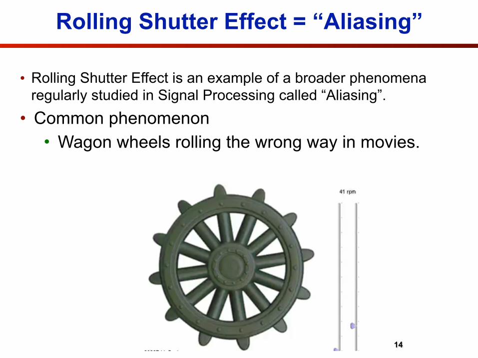
Rolling Shutter Effect = “Aliasing”

• Rolling Shutter Effect is an example of a broader phenomena regularly studied in Signal Processing called “Aliasing”.

• Common phenomenon • Wagon wheels rolling the wrong way in movies.

14

Rolling Shutter Effect = “Aliasing”

• Rolling Shutter Effect is an example of a broader phenomena regularly studied in Signal Processing called “Aliasing”.

• Common phenomenon • Wagon wheels rolling the wrong way in movies.

14

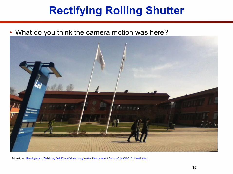
Rectifying Rolling Shutter

• What do you think the camera motion was here?

15

Stabilizing Cell Phone Video using Inertial Measurement Sensors

Gustav Hanning, Nicklas Forslow, Per-Erik Forssen, Erik Ringaby, David Tornqvist, Jonas CallmerDepartment of Electrical Engineering

Linkoping Universityhttp://www.liu.se/forskning/foass/per-erik-forssen/VGS

Abstract

We present a system that rectifies and stabilizes video

sequences on mobile devices with rolling-shutter cameras.

The system corrects for rolling-shutter distortions using

measurements from accelerometer and gyroscope sensors,

and a 3D rotational distortion model. In order to obtain

a stabilized video, and at the same time keep most content

in view, we propose an adaptive low-pass filter algorithm

to obtain the output camera trajectory. The accuracy of the

orientation estimates has been evaluated experimentally us-

ing ground truth data from a motion capture system. We

have conducted a user study, where the output from our sys-

tem, implemented in iOS, has been compared to that of three

other applications, as well as to the uncorrected video. The

study shows that users prefer our sensor-based system.

1. Introduction

Most mobile video-recording devices of today make useof CMOS sensors with rolling-shutter (RS) readout [6]. AnRS camera captures video by exposing every frame line-by-line from top to bottom. This is in contrast to a global shut-

ter, where an entire frame is acquired at once.The RS technique gives rise to image distortions in sit-

uations where either the device or the target is moving.Figure 1 shows an example of how an image is distortedwhen using a rolling shutter. Here, vertical lines such asthe flag poles appear slanted as a result of panning the cam-era quickly from left to right during recording. Recordingvideo by hand also leads to visible frame-to-frame jitter.The recorded video is perceived as “shaky” and is not veryenjoyable to watch.

Since mobile video-recording devices are so common,there is an interest in correcting these types of distor-tions. The inertial sensors (accelerometers and gyroscopes)present in many of the new devices provide a new way ofdoing this: Using the position and/or orientation of the de-vice, as sensed during recording, the motion induced distor-tions can be compensated for in a post-processing step.

Figure 1. An example of rolling-shutter distortion. Top: Frame

from a video sequence recorded with an iPod touch. Bottom: Rec-

tification using the 3D rotation model and inertial measurements.

1.1. Related Work

Early work on modeling the distortions caused by arolling-shutter exposure is described in [7].

Rolling-shutter video has previously been rectified usingimage measurements. Two recent, state-of-the-art methodsare described in [3, 5]. To perform rectification, we usethe 3D rotational model introduced in [5], but use inertialsensor data instead of image measurements.

For stabilization we use a 3D rotation-based correctionas in [13, 14], and a dynamical model derived from [17].Differences compared to [13, 14] is the use of inertial sen-sor data instead of image measurements, and an adaptive

1

Taken from: Hanning et al. “Stabilizing Cell Phone Video using Inertial Measurement Sensors” in ICCV 2011 Workshop.

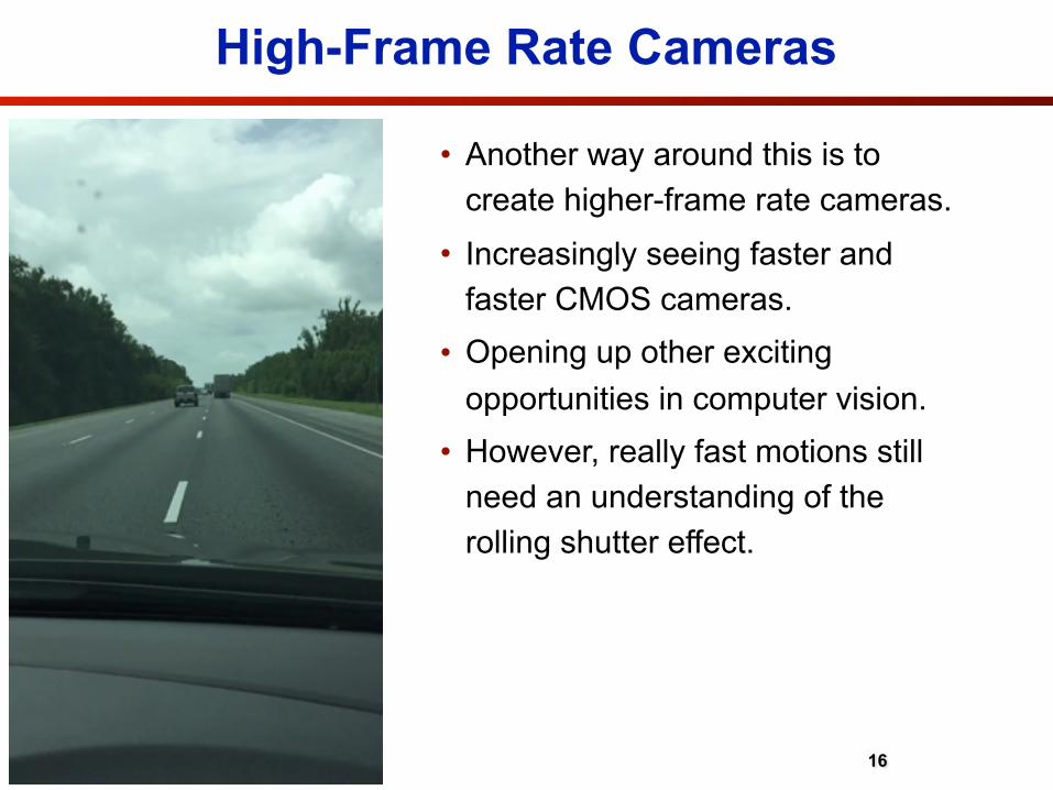
High-Frame Rate Cameras

• Another way around this is to create higher-frame rate cameras.

• Increasingly seeing faster and faster CMOS cameras.

• Opening up other exciting opportunities in computer vision.

• However, really fast motions still need an understanding of the rolling shutter effect.

16

High-Frame Rate Cameras

• Another way around this is to create higher-frame rate cameras.

• Increasingly seeing faster and faster CMOS cameras.

• Opening up other exciting opportunities in computer vision.

• However, really fast motions still need an understanding of the rolling shutter effect.

16

Rectifying Rolling Shutter

• Result from rectification,

17

Taken from: Hanning et al. “Stabilizing Cell Phone Video using Inertial Measurement Sensors” in ICCV 2011 Workshop.

Stabilizing Cell Phone Video using Inertial Measurement Sensors

Gustav Hanning, Nicklas Forslow, Per-Erik Forssen, Erik Ringaby, David Tornqvist, Jonas CallmerDepartment of Electrical Engineering

Linkoping Universityhttp://www.liu.se/forskning/foass/per-erik-forssen/VGS

Abstract

We present a system that rectifies and stabilizes video

sequences on mobile devices with rolling-shutter cameras.

The system corrects for rolling-shutter distortions using

measurements from accelerometer and gyroscope sensors,

and a 3D rotational distortion model. In order to obtain

a stabilized video, and at the same time keep most content

in view, we propose an adaptive low-pass filter algorithm

to obtain the output camera trajectory. The accuracy of the

orientation estimates has been evaluated experimentally us-

ing ground truth data from a motion capture system. We

have conducted a user study, where the output from our sys-

tem, implemented in iOS, has been compared to that of three

other applications, as well as to the uncorrected video. The

study shows that users prefer our sensor-based system.

1. Introduction

Most mobile video-recording devices of today make useof CMOS sensors with rolling-shutter (RS) readout [6]. AnRS camera captures video by exposing every frame line-by-line from top to bottom. This is in contrast to a global shut-

ter, where an entire frame is acquired at once.The RS technique gives rise to image distortions in sit-

uations where either the device or the target is moving.Figure 1 shows an example of how an image is distortedwhen using a rolling shutter. Here, vertical lines such asthe flag poles appear slanted as a result of panning the cam-era quickly from left to right during recording. Recordingvideo by hand also leads to visible frame-to-frame jitter.The recorded video is perceived as “shaky” and is not veryenjoyable to watch.

Since mobile video-recording devices are so common,there is an interest in correcting these types of distor-tions. The inertial sensors (accelerometers and gyroscopes)present in many of the new devices provide a new way ofdoing this: Using the position and/or orientation of the de-vice, as sensed during recording, the motion induced distor-tions can be compensated for in a post-processing step.

Figure 1. An example of rolling-shutter distortion. Top: Frame

from a video sequence recorded with an iPod touch. Bottom: Rec-

tification using the 3D rotation model and inertial measurements.

1.1. Related Work

Early work on modeling the distortions caused by arolling-shutter exposure is described in [7].

Rolling-shutter video has previously been rectified usingimage measurements. Two recent, state-of-the-art methodsare described in [3, 5]. To perform rectification, we usethe 3D rotational model introduced in [5], but use inertialsensor data instead of image measurements.

For stabilization we use a 3D rotation-based correctionas in [13, 14], and a dynamical model derived from [17].Differences compared to [13, 14] is the use of inertial sen-sor data instead of image measurements, and an adaptive

1

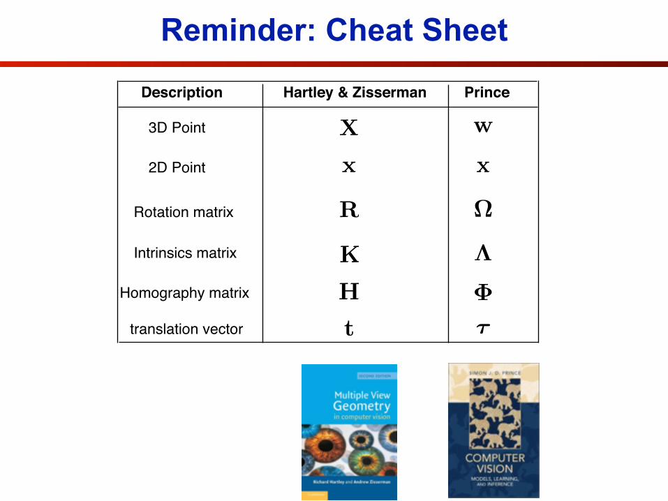
Reminder: Cheat Sheet

Hartley & Zisserman PrinceDescription

3D Point X

2D Point x

w

x

Rotation matrix R

Intrinsics matrix K

⌦

�

⇤

Homography matrix H

translation vector t ⌧

First camera:

Second camera:

Substituting:

This is a mathematical relationship between the points in the two images, but it’s not in the most convenient form.

Reminder: The Essential Matrix

Adapted from: Computer vision: models, learning and inference. Simon J.D. Prince

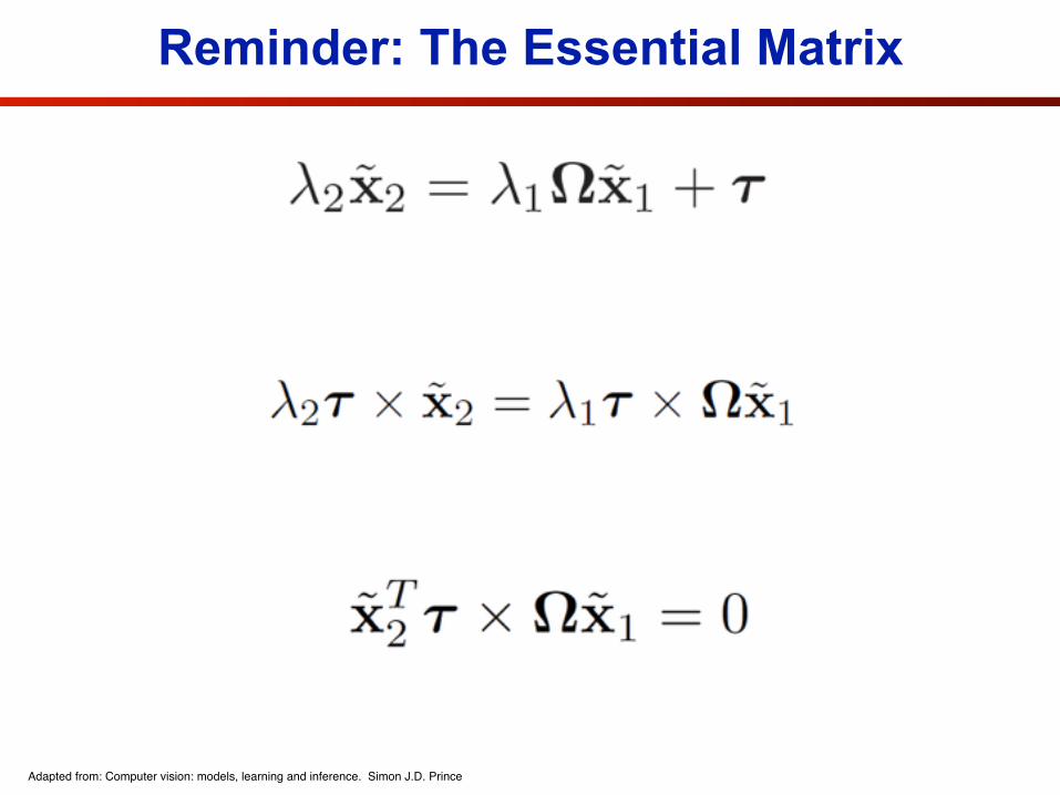
Reminder: The Essential Matrix

Adapted from: Computer vision: models, learning and inference. Simon J.D. Prince

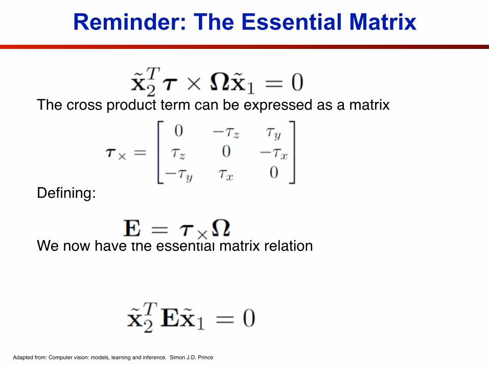
The cross product term can be expressed as a matrix

Defining:

We now have the essential matrix relation

Reminder: The Essential Matrix

Adapted from: Computer vision: models, learning and inference. Simon J.D. Prince

Epipolar Geometry for Rolling Shutter

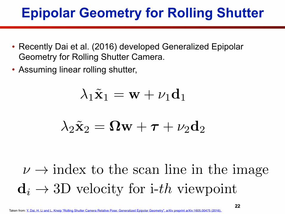
• Recently Dai et al. (2016) developed Generalized Epipolar Geometry for Rolling Shutter Camera.

• Assuming linear rolling shutter,

22Taken from: Y. Dai, H. Li and L. Kneip “Rolling Shutter Camera Relative Pose: Generalized Epipolar Geometry”, arXiv preprint arXiv:1605.00475 (2016).

�1x1 = w + ⌫1d1

�2x2 = ⌦w + ⌧ + ⌫2d2

⌫ ! index to the scan line in the image

di ! 3D velocity for i-th viewpoint

Epipolar Geometry for Rolling Shutter

• Results in a different essential matrix for every possible combination of and .

23

⌫1 ⌫2

[u0i, v

0i, 1]

T , we have the standard essential matrix constrain-t: x

0Ti Exi = 0. From a sufficient number of correspon-

dences one can solve for E. Once E is obtained, decom-posing E according to E = [t]⇥R leads to the relative pose(i.e. R and t).

For a rolling-shutter camera, unfortunately, such a glob-al 3-by-3 essential matrix does not exist. This is primarilybecause an RS camera is not a central projection camera;every scanline has its own distinct local pose. As a result,every pair of feature correspondences may give rise to a d-ifferent “essential matrix”. Formally, for xi $ x

0i, we have

x

0Ti Eui,u0

ixi = 0. (5)

Note that E is dependent of the scanlines ui and u0i. In other

words, there does not exist a single global 3 ⇥ 3 essentialmatrix for a pair of RS images.

Figure-2 shows that despite the fact that different scan-lines possess different centers of projection, for a pair offeature correspondences the co-planarity relationship stillholds, because the two feature points in image planes corre-spond to the same 3D point in space. As such, the concep-t of two-view epipolar relationship should still exist. Ournext task is to derive such a generalized epipolar relation.

Figure 2. This figure shows that different scanlines in a RS imagehave different effective optical centers. For any pair of feature cor-respondences (indicated by red ‘x’s in the picture), a co-planarityrelationship however still holds.

Given two scanlines ui, uj and the corresponding cameraposes Pui = [Rui , tui ] and Puj = [Ruj , tuj ], we have

Euiuj = [tuj �RujRTuitui ]⇥RujR

Tui. (6)

Rolling Shutter Relative Pose. Note, given a pair of fea-ture correspondences xi $ x

0i, one can establish the fol-

lowing RS epipolar equation: x0Ti Euiu0

ixi = 0. Given suffi-

cient pairs of correspondences; each pair contributes to oneequation over the unknown parameters; our goal is to solvefor the relative pose between the two RS images.

We set the first camera’s pose at [I,0], and the secondcamera at [R, t]. We denote the two cameras’ inter-scanlinerotational (angular) velocities as w1, and w2, and their lin-ear translational velocities as d1 and d2. Taking a uniformRS camera as an example, the task of rolling shutter rela-tive pose is to find the unknowns {R, t,w1,w2,d1,d2}.

In total there are 2 ⇥ 12 � 6 � 1 = 17 non-trivial vari-ables (excluding the gauge freedom of the first camera, anda global scale). Collecting at least 17 equations in generalconfiguration, it is possible to solve this system of (gener-ally nonlinear) equations over the 17 unknown parameters.In this paper, we will show how to derive linear N-point al-gorithms for rolling shutter cameras, as an analogy to thelinear 8-point algorithm for the case of a pinhole camera.

4. Rolling-Shutter Essential MatricesIn this section, we will generalize the conventional 3⇥ 3

essential matrix for perspective cameras to 4⇥4, 5⇥5, 6⇥6,and 7 ⇥ 7 matrices for different types of Rolling-Shutter(RS) and Push-Broom (PB) cameras. The reason for in-cluding push-broom cameras will be made clear soon.

4.1. A 5⇥ 5 essential matrix for linear RS cameras

For a linear rolling shutter camera, since the inter-scanline motion is a pure translation, there are four parame-ter vectors to be estimated, namely{R, t,d1,d2}. The totaldegree of freedom of the unknowns is 3+3+3+3�1 = 11.(the last ‘-1’ accounts for a global scale).

The epipolarity defined between the ui-th scanline of thefirst RS frame and the u0

i-th scanline of the second RS frameis represented as Euiu0

i= [tuiu0

i]⇥Ruiu0

i, where the trans-

lation tuiu0i= t+ u0

id2 � uiRd1. This translates into

2

4u0i

v0i1

3

5T

[t+ u0id2 � uiRd1]⇥R

2

4ui

vi1

3

5= 0. (7)

Expanding this scanline epipolar equation, one can obtainthe following 5⇥ 5 matrix form:

2

666664

u02i

u0iv

0i

u0i

v0i1

3

777775

T 2

6664

0 0 f13 f14 f150 0 f23 f24 f25f31 f32 f33 f34 f35f41 f42 f43 f44 f45f51 f52 f53 f54 f55

3

7775

2

6664

u2i

uiviui

vi1

3

7775= 0,

(8)where the entries of the 5⇥5 matrix F = [fi,j ] are functionsof the 11 unknown parameters {R, t,d1,d2}. In total, thereare 21 homogeneous variables, thus a linear 20-point solvermust exist to solve for this hyperbolic essential matrix.

Proof. By redefining d1 Rd1, we easily obtain

Euiu0i

= ([t]⇥ + u0i[d2]⇥ � ui[d1]⇥)R. (9)

Denoting E0 = [t]⇥R, E1 = [d1]⇥R and E2 = [d2]⇥R,we have:

[u0i, v

0i, 1](E0 + u0

iE2 � uiE1)[ui, vi, 1]T= 0. (10)

Taken from: Y. Dai, H. Li and L. Kneip “Rolling Shutter Camera Relative Pose: Generalized Epipolar Geometry”, arXiv preprint arXiv:1605.00475 (2016).

E(⌫1, ⌫2) = (⌧ + ⌫2d2 � ⌫1⌦d1)⇥⌦

Epipolar Geometry for Rolling Shutter

• Results in a different essential matrix for every possible combination of and .

23

⌫1 ⌫2

[u0i, v

0i, 1]

T , we have the standard essential matrix constrain-t: x

0Ti Exi = 0. From a sufficient number of correspon-

dences one can solve for E. Once E is obtained, decom-posing E according to E = [t]⇥R leads to the relative pose(i.e. R and t).

For a rolling-shutter camera, unfortunately, such a glob-al 3-by-3 essential matrix does not exist. This is primarilybecause an RS camera is not a central projection camera;every scanline has its own distinct local pose. As a result,every pair of feature correspondences may give rise to a d-ifferent “essential matrix”. Formally, for xi $ x

0i, we have

x

0Ti Eui,u0

ixi = 0. (5)

Note that E is dependent of the scanlines ui and u0i. In other

words, there does not exist a single global 3 ⇥ 3 essentialmatrix for a pair of RS images.

Figure-2 shows that despite the fact that different scan-lines possess different centers of projection, for a pair offeature correspondences the co-planarity relationship stillholds, because the two feature points in image planes corre-spond to the same 3D point in space. As such, the concep-t of two-view epipolar relationship should still exist. Ournext task is to derive such a generalized epipolar relation.

Figure 2. This figure shows that different scanlines in a RS imagehave different effective optical centers. For any pair of feature cor-respondences (indicated by red ‘x’s in the picture), a co-planarityrelationship however still holds.

Given two scanlines ui, uj and the corresponding cameraposes Pui = [Rui , tui ] and Puj = [Ruj , tuj ], we have

Euiuj = [tuj �RujRTuitui ]⇥RujR

Tui. (6)

Rolling Shutter Relative Pose. Note, given a pair of fea-ture correspondences xi $ x

0i, one can establish the fol-

lowing RS epipolar equation: x0Ti Euiu0

ixi = 0. Given suffi-

cient pairs of correspondences; each pair contributes to oneequation over the unknown parameters; our goal is to solvefor the relative pose between the two RS images.

We set the first camera’s pose at [I,0], and the secondcamera at [R, t]. We denote the two cameras’ inter-scanlinerotational (angular) velocities as w1, and w2, and their lin-ear translational velocities as d1 and d2. Taking a uniformRS camera as an example, the task of rolling shutter rela-tive pose is to find the unknowns {R, t,w1,w2,d1,d2}.

In total there are 2 ⇥ 12 � 6 � 1 = 17 non-trivial vari-ables (excluding the gauge freedom of the first camera, anda global scale). Collecting at least 17 equations in generalconfiguration, it is possible to solve this system of (gener-ally nonlinear) equations over the 17 unknown parameters.In this paper, we will show how to derive linear N-point al-gorithms for rolling shutter cameras, as an analogy to thelinear 8-point algorithm for the case of a pinhole camera.

4. Rolling-Shutter Essential MatricesIn this section, we will generalize the conventional 3⇥ 3

essential matrix for perspective cameras to 4⇥4, 5⇥5, 6⇥6,and 7 ⇥ 7 matrices for different types of Rolling-Shutter(RS) and Push-Broom (PB) cameras. The reason for in-cluding push-broom cameras will be made clear soon.

4.1. A 5⇥ 5 essential matrix for linear RS cameras

For a linear rolling shutter camera, since the inter-scanline motion is a pure translation, there are four parame-ter vectors to be estimated, namely{R, t,d1,d2}. The totaldegree of freedom of the unknowns is 3+3+3+3�1 = 11.(the last ‘-1’ accounts for a global scale).

The epipolarity defined between the ui-th scanline of thefirst RS frame and the u0

i-th scanline of the second RS frameis represented as Euiu0

i= [tuiu0

i]⇥Ruiu0

i, where the trans-

lation tuiu0i= t+ u0

id2 � uiRd1. This translates into

2

4u0i

v0i1

3

5T

[t+ u0id2 � uiRd1]⇥R

2

4ui

vi1

3

5= 0. (7)

Expanding this scanline epipolar equation, one can obtainthe following 5⇥ 5 matrix form:

2

666664

u02i

u0iv

0i

u0i

v0i1

3

777775

T 2

6664

0 0 f13 f14 f150 0 f23 f24 f25f31 f32 f33 f34 f35f41 f42 f43 f44 f45f51 f52 f53 f54 f55

3

7775

2

6664

u2i

uiviui

vi1

3

7775= 0,

(8)where the entries of the 5⇥5 matrix F = [fi,j ] are functionsof the 11 unknown parameters {R, t,d1,d2}. In total, thereare 21 homogeneous variables, thus a linear 20-point solvermust exist to solve for this hyperbolic essential matrix.

Proof. By redefining d1 Rd1, we easily obtain

Euiu0i

= ([t]⇥ + u0i[d2]⇥ � ui[d1]⇥)R. (9)

Denoting E0 = [t]⇥R, E1 = [d1]⇥R and E2 = [d2]⇥R,we have:

[u0i, v

0i, 1](E0 + u0

iE2 � uiE1)[ui, vi, 1]T= 0. (10)

Taken from: Y. Dai, H. Li and L. Kneip “Rolling Shutter Camera Relative Pose: Generalized Epipolar Geometry”, arXiv preprint arXiv:1605.00475 (2016).

How many degrees of freedom?

E(⌫1, ⌫2) = (⌧ + ⌫2d2 � ⌫1⌦d1)⇥⌦

Epipolar Geometry for Rolling Shutter

24

Table 1. A hierarchy of generalized essential matrices for different types of rolling-shutter and push-broom cameras.Camera Model Essential Matrix Monomials Degree-of-freedom Linear Algorithm Non-linear Algorithm Motion Parameters

Perspective camera

2

4f11 f12 f13f21 f22 f23f31 f32 f33

3

5 (ui, vi, 1) 32 = 9 8-point 5-point R, t

Linear push broom

2

664

0 0 f13 f140 0 f23 f24f31 f32 f33 f34f41 f42 f43 f44

3

775 (uivi, ui, vi, 1) 12 = 42 � 22 11-point 11-point R, t,d1,d2

Linear rolling shutter

2

6664

0 0 f13 f14 f150 0 f23 f24 f25f31 f32 f33 f34 f35f41 f42 f43 f44 f45f51 f52 f53 f54 f55

3

7775(u2

i , uivi, ui, vi, 1) 21 = 52 � 22 20-point 11-point R, t,d1,d2

Uniform push broom

2

666664

0 0 f13 f14 f15 f160 0 f23 f24 f25 f26f31 f32 f33 f34 f35 f36f41 f42 f43 f44 f45 f46f51 f52 f53 f54 f55 f56f61 f62 f63 f64 f65 f66

3

777775(u2

i vi, u2i , uivi, ui, vi, 1) 32 = 62 � 22 31-point 17-point R, t,w1,w2,d1,d2

Uniform rolling shutter

2

66666664

0 0 f13 f14 f15 f16 f170 0 f23 f24 f25 f26 f27f31 f32 f33 f34 f35 f36 f37f41 f42 f43 f44 f45 f46 f47f51 f52 f53 f54 f55 f56 f57f61 f62 f63 f64 f65 f66 f67f71 f72 f73 f74 f75 f76 f77

3

77777775

(u3i , u

2i vi, u

2i , uivi, ui, vi, 1) 45 = 72 � 22 44-point 17-point R, t,w1,w2,d1,d2

sential matrices, we can easily develop efficient numericalalgorithms to solve the rolling shutter relative pose prob-lem. Similar to the 8-point linear algorithm in the perspec-tive case, we derive a 20-point linear algorithm for linearRS cameras, and a 44-point linear algorithm for uniformRS cameras. We also develop non-linear solvers for bothcases (by minimizing the geometrically meaningful Samp-son error). Our non-linear solvers work for the minimumnumber of feature points, hence are relevant for RANSAC.

Experiments on both synthetic RS datasets and real RSimages have validated the proposed theory and algorithm-s. To the best of our knowledge, this is the first work thatprovides a unified framework and practical solutions to therolling shutter relative pose problem. Our 5 ⇥ 5 and 7 ⇥ 7

RS essential matrices are original; they were not reportedbefore in computer vision literature. Inspired by this suc-cess, we further discover that there also exist practicallymeaningful 4⇥ 4 and 6⇥ 6 generalized essential matrices,corresponding to linear, and uniform push-broom cameras,respectively. Together, this paper provides a unified frame-work for solving the relative pose problems with rolling-shutter or push-broom cameras under different yet practi-cally relevant conditions. It also provides new geometricinsights into the connection between different types of nov-el camera geometries.

Table-1 gives a brief summary of the new results discov-ered in this paper. Details will be explained in Section-4.

1.1. Related work

The present work discusses a fundamental geometricproblem in the context of rolling shutter cameras. Themost notable, early related work is by Geyer et al. [16],which proposes a projection model for rolling shutter cam-eras based on a constant velocity motion model. This fun-damental idea of a compact, local expression of camer-a dynamics has regained interest through Ait-Aider et al.

[1], who solved the absolute pose problem through itera-tive minimization, and for the first time described the higherdensity of the temporal sampling of a rolling shutter mech-anism as an advantage rather than a disadvantage. Albl etal.[3] proposed a two-step procedure in which the pose isfirst initialized using a global shutter model, and then re-fined based on a rolling shutter model and a small-rotationapproximation. Saurer et al. [22] solved the problem in asingle shot, however under the simplifying assumption thatthe rotational velocity of the camera is zero. Sunghoon etal. [11] also employed a linear model, however with the fi-nal goal of dense depth estimation from stereo. Grundmannet al. proposed a method to automatic rectify rolling shutterdistortion from feature correspondences only [5]. To date,a single-shot, closed-form solution to compute the relativepose for a rolling shutter camera remains an open problem,thus underlining the difficulty of the geometry even in thefirst-order case.

Rolling shutter cameras can be regarded as generalmulti-perspective cameras, and are thus closely related toseveral other camera models. For instance, Gupta and Hart-ley [6] introduced the linear push-broom model where—similar to rolling shutter cameras—the vertical image coor-dinate becomes correlated to the time at which the corre-sponding row is sampled. This notably leads to a quadrat-ic essential polynomial and a related, higher-order essen-tial matrix. We establish the close link to this model andcontribute to the classification in [27] by presenting a novelhierarchy of higher order generalized essential matrices.

Moving towards iterative non-linear refinement method-s permits a more general inclusion of higher-order motionmodels. Hedborg et al. [9, 10] introduced a bundle ad-justment framework for rolling shutter cameras by relyingon the SLERP model for interpolating rotations. Magarandet al. [15] introduced an approach for global optimizationof pose and dynamics from a single rolling shutter image.

Taken from: Y. Dai, H. Li and L. Kneip “Rolling Shutter Camera Relative Pose: Generalized Epipolar Geometry”, arXiv preprint arXiv:1605.00475 (2016).

Accessing the Camera in iOS

25

Accessing the Camera in iOS

25

Accessing the Camera in iOS

25

Today

• CCD vs CMOS cameras.

• Rolling Shutter Epipolar Geometry

• Inertial Measurement Units (IMU)

Inertial Measurement Unit• Measures a device’s specific force, angular rate & magnetic field. • Composed of,

• Accelerometer. • Gyroscope. • Magnetometer.

• Historically used heavily within navigation and robotic systems. • More recently have become common place in smart devices.

27

Accelerometer

28

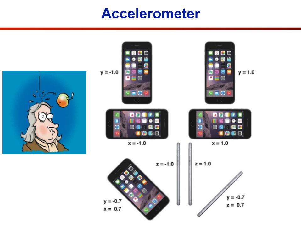
Accelerometer

28

Accelerometer

28What can’t you measure?

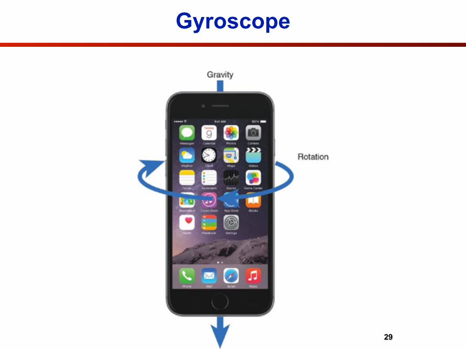
Gyroscope

29

IMU Example in iOS

• Good example of using IMU in iOS can be found at,

https://github.com/nscookbook/recipe19

• Or better yet, if you have git installed you can type from the command line.

$ git clone https://github.com/NSCookbook/recipe19.git

• Good tutorial about how code works can be found at,

http://nscookbook.com/2013/03/ios-programming-recipe-19-using-core-motion-to-access-gyro-and-accelerometer/

Accessing the IMU in iOS

31

Accessing the IMU in iOS

31

Accessing the IMU in iOS

31

Accessing the IMU in iOS

31

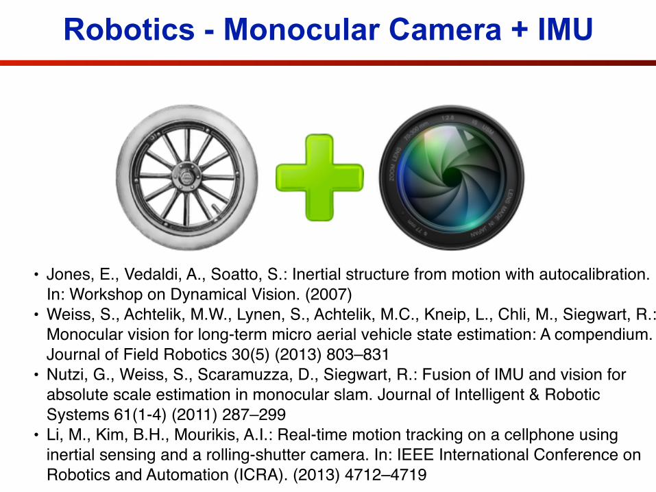
Robotics - Monocular Camera + IMU

• Jones, E., Vedaldi, A., Soatto, S.: Inertial structure from motion with autocalibration. In: Workshop on Dynamical Vision. (2007)

• Weiss, S., Achtelik, M.W., Lynen, S., Achtelik, M.C., Kneip, L., Chli, M., Siegwart, R.: Monocular vision for long-term micro aerial vehicle state estimation: A compendium. Journal of Field Robotics 30(5) (2013) 803–831

• Nutzi, G., Weiss, S., Scaramuzza, D., Siegwart, R.: Fusion of IMU and vision for absolute scale estimation in monocular slam. Journal of Intelligent & Robotic Systems 61(1-4) (2011) 287–299

• Li, M., Kim, B.H., Mourikis, A.I.: Real-time motion tracking on a cellphone using inertial sensing and a rolling-shutter camera. In: IEEE International Conference on Robotics and Automation (ICRA). (2013) 4712–4719

Mobile Solutions

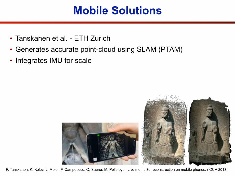
• Tanskanen et al. - ETH Zurich • Generates accurate point-cloud using SLAM (PTAM) • Integrates IMU for scale

P. Tanskanen, K. Kolev, L. Meier, F. Camposeco, O. Saurer, M. Pollefeys : Live metric 3d reconstruction on mobile phones. (ICCV 2013)

Mobile Visual SLAM + IMU

P. Tanskanen, K. Kolev, L. Meier, F. Camposeco, O. Saurer, M. Pollefeys : Live metric 3d reconstruction on mobile phones. (ICCV 2013)

Mobile Visual SLAM + IMU

P. Tanskanen, K. Kolev, L. Meier, F. Camposeco, O. Saurer, M. Pollefeys : Live metric 3d reconstruction on mobile phones. (ICCV 2013)

Mobile Visual SLAM + IMU

P. Tanskanen, K. Kolev, L. Meier, F. Camposeco, O. Saurer, M. Pollefeys : Live metric 3d reconstruction on mobile phones. (ICCV 2013)

35C. Ham, S. Singh, and S. Lucey: Handwaving away scale. (ECCV 2014)

35C. Ham, S. Singh, and S. Lucey: Handwaving away scale. (ECCV 2014)

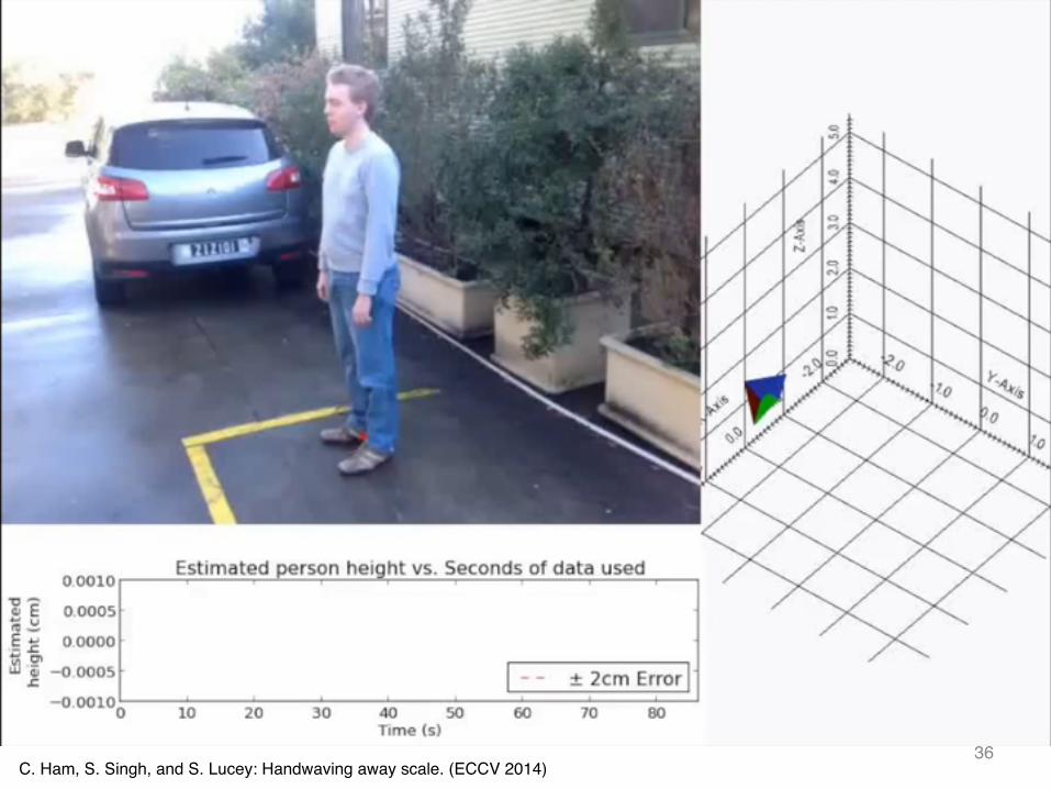
36C. Ham, S. Singh, and S. Lucey: Handwaving away scale. (ECCV 2014)

36C. Ham, S. Singh, and S. Lucey: Handwaving away scale. (ECCV 2014)

37C. Ham, S. Singh, and S. Lucey: Handwaving away scale. (ECCV 2014)

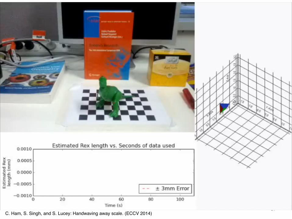
37C. Ham, S. Singh, and S. Lucey: Handwaving away scale. (ECCV 2014)

Mobile Platform Issues

• IMU and Camera time stamped differently

IMU (System timestamps)

Camera(Relative timestamps)

1045 ns

0 ns

1145 ns

100 ns

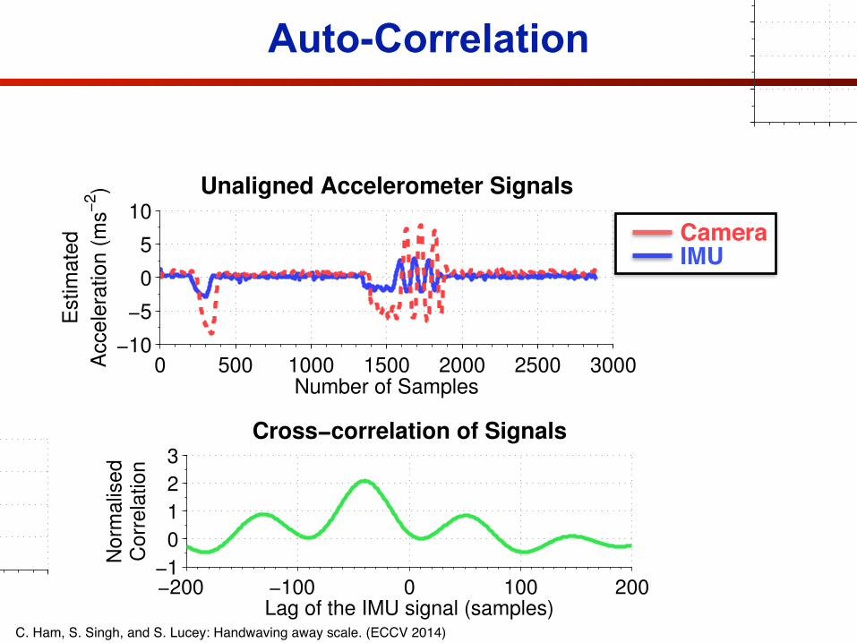
Hand Waving Away Scale 7

0 500 1000 1500 2000 2500 3000−10

−5

0

5

10Unaligned Accelerometer Signals

Number of Samples

Est

ima

ted

Acc

ele

ratio

n (

ms−

2)

−200 −100 0 100 200−1

0

1

2

3Cross−correlation of Signals

Lag of the IMU signal (samples)

No

rma

lise

dC

orr

ela

tion

0 500 1000 1500 2000 2500 3000−10

−5

0

5

10Unaligned Accelerometer Signals

Number of Samples

Est

ima

ted

Acc

ele

ratio

n (

ms−

2)

−200 −100 0 100 200−1

0

1

2

3Cross−correlation of Signals

Lag of the IMU signal (samples)

No

rma

lise

dC

orr

ela

tion

Fig. 2: Showing the result of the normalised cross-correlation of the camera and IMUsignals. Blue-solid line: camera acceleration scaled by initial solution. Red-dashed line:IMU acceleration. The delay that gives the best alignment here is approximately 40samples.

3.4 Gravity as a FriendThe above method for finding the delay between two signals can struggle with smallermotions when data is particularly noisy. Reintroducing gravity has two advantages: (i)it behaves as an anchor to significantly improve the robustness of the alignment, (ii)allows us to remove the black box gravity estimation built in to smart devices withIMUs.

Instead of comparing the estimated camera acceleration and linear IMU accelera-tion, we add the gravity vector, g, back into the camera acceleration and compare it withthe raw IMU acceleration (which already contains gravity). Grabity is oriented, muchlike the vision acceleration, with the IMU acceleration before superimposing

G =

0

B@g

|R

V

1...

g

|R

V

F

1

CA . (6)

0 200 400 600 800−5

0

5Gravity vs. No Gravity in IMU Acceleration

Acc

ele

ratio

n (

ms−

2)

Number of Samples

Fig. 3: The large, low frequency motions of rotation through the gravity field helpsanchor the temporal alignment. Blue solid line: IMU acceleration with gravity removed.Red dashed line: raw IMU acceleration measuring gravity.

Since the accelerations are in the camera reference frame the reintroduction of grav-ity essentially captures the pitch and roll of the smart device. The red dashed line in

Auto-Correlation

Hand Waving Away Scale 7

0 500 1000 1500 2000 2500 3000−10

−5

0

5

10Unaligned Accelerometer Signals

Number of Samples

Est

ima

ted

Acc

ele

ratio

n (

ms−

2)

−200 −100 0 100 200−1

0

1

2

3Cross−correlation of Signals

Lag of the IMU signal (samples)

No

rma

lise

dC

orr

ela

tion

0 500 1000 1500 2000 2500 3000−10

−5

0

5

10Unaligned Accelerometer Signals

Number of Samples

Est

ima

ted

Acc

ele

ratio

n (

ms−

2)

−200 −100 0 100 200−1

0

1

2

3Cross−correlation of Signals

Lag of the IMU signal (samples)

No

rma

lise

dC

orr

ela

tion

Fig. 2: Showing the result of the normalised cross-correlation of the camera and IMUsignals. Blue-solid line: camera acceleration scaled by initial solution. Red-dashed line:IMU acceleration. The delay that gives the best alignment here is approximately 40samples.

3.4 Gravity as a FriendThe above method for finding the delay between two signals can struggle with smallermotions when data is particularly noisy. Reintroducing gravity has two advantages: (i)it behaves as an anchor to significantly improve the robustness of the alignment, (ii)allows us to remove the black box gravity estimation built in to smart devices withIMUs.

Instead of comparing the estimated camera acceleration and linear IMU accelera-tion, we add the gravity vector, g, back into the camera acceleration and compare it withthe raw IMU acceleration (which already contains gravity). Grabity is oriented, muchlike the vision acceleration, with the IMU acceleration before superimposing

G =

0

B@g

|R

V

1...

g

|R

V

F

1

CA . (6)

0 200 400 600 800−5

0

5Gravity vs. No Gravity in IMU Acceleration

Acc

ele

ratio

n (

ms−

2)

Number of Samples

Fig. 3: The large, low frequency motions of rotation through the gravity field helpsanchor the temporal alignment. Blue solid line: IMU acceleration with gravity removed.Red dashed line: raw IMU acceleration measuring gravity.

Since the accelerations are in the camera reference frame the reintroduction of grav-ity essentially captures the pitch and roll of the smart device. The red dashed line in

CameraIMU

C. Ham, S. Singh, and S. Lucey: Handwaving away scale. (ECCV 2014)

More to read…

• Y. Dai, H. Li and L. Kneip “Rolling Shutter Camera Relative Pose: Generalized Epipolar Geometry”, arXiv preprint arXiv:1605.00475 (2016).

Rolling Shutter Camera Relative Pose: Generalized Epipolar Geometry

Yuchao Dai1, Hongdong Li1,2 and Laurent Kneip1,2

1 Research School of Engineering, Australian National University2ARC Centre of Excellence for Robotic Vision (ACRV)

Abstract

The vast majority of modern consumer-grade camerasemploy a rolling shutter mechanism. In dynamic geomet-ric computer vision applications such as visual SLAM, theso-called rolling shutter effect therefore needs to be prop-erly taken into account. A dedicated relative pose solverappears to be the first problem to solve, as it is of eminentimportance to bootstrap any derivation of multi-view ge-ometry. However, despite its significance, it has receivedinadequate attention to date.

This paper presents a detailed investigation of the ge-ometry of the rolling shutter relative pose problem. We in-troduce the rolling shutter essential matrix, and establishits link to existing models such as the push-broom cameras,summarized in a clean hierarchy of multi-perspective cam-eras. The generalization of well-established concepts fromepipolar geometry is completed by a definition of the Samp-son distance in the rolling shutter case. The work is con-cluded with a careful investigation of the introduced epipo-lar geometry for rolling shutter cameras on several dedicat-ed benchmarks.

1. IntroductionRolling-Shutter (RS) CMOS cameras are getting more

and more popularly used in real-world computer vision ap-plications due to their low cost and simplicity in design. Touse these cameras in 3D geometric computer vision tasks(such as 3D reconstruction, object pose, visual SLAM),the rolling shutter effect (e.g. wobbling) must be careful-ly accounted for. Simply ignoring this effect and relyingon a global-shutter method may lead to erroneous, undesir-able and distorted results as reported in previous work (e.g.[11, 13, 3]).

Recently, many classic 3D vision algorithms have beenadapted to the rolling shutter case (e.g. absolute Pose [15][3] [22], Bundle Adjustment [9], and stereo rectification[21]). Quite surprisingly, no previous attempt has been re-ported on solving the relative pose problem with a RollingShutter (RS) camera.

(a) linear RS (b) uniform RS

(c) linear PB (d) uniform PB

Figure 1. Example epipolar curves for the camera models dis-cussed in this paper. Groups of epipolar curves of identical col-or originate from points on the same row in another image, whileboth images are under motion. For linear rolling shutter (a) andlinear push broom cameras (c), the epipolar curves are conic. Theepipolar curves for uniform rolling shutter (b) and uniform pushbroom cameras (d) are cubic.

The complexity of this problem stems from the fact thata rolling shutter camera does not satisfy the pinhole projec-tion model, hence the conventional epipolar geometry de-fined by the standard 3 ⇥ 3 essential matrix (in the form ofx

0TEx = 0) is no longer applicable. This is mainly because

of the time-varying scaneline-by-scanline image capturingnature of an RS camera, rendering the imaging process anon-central one.

In this paper we show that similar epipolar relationshipsdo exist between two rolling-shutter images. Specifically,in contrast to the conventional 3 ⇥ 3 essential matrix forthe pinhole camera, we derive a 7⇥ 7 generalized essentialmatrix for a uniform rolling-shutter camera, and a 5⇥5 gen-eralized essential matrix for a linear rolling-shutter camera.Another result is that, under the rolling-shutter epipolar ge-ometry, the “epipolar lines” are no longer straight lines, butbecome higher-order “epipolar curves” (c.f . Fig. 1).

Armed with these novel generalized rolling-shutter es-

arX

iv:1

605.

0047

5v1

[cs.C

V]

2 M

ay 2

016