* All errors are our own. The views we express herein are not necessarily those of the Board of Governors or others within the Federal Reserve System. We thank the Guthrie Center for Real Estate Research for financial support and seminar and conference participants at Kellogg, UBC‐Sauder, George Washington,  the DC Urban Day,  the Urban Institute, and the Urban Economics Association for helpful comments. 

Housing Supply and Affordability* 

 

 

Raven Molloy 

Federal Reserve Board 

 

Charles G. Nathanson 

Northwestern University 

 

Andrew Paciorek 

Federal Reserve Board 

 

 

 

August 2019 

 

We examine how housing supply constraints affect housing affordability, which we define as the 

quality‐adjusted price of housing services. Our dynamic model predicts that supply constraints 

will increase the price of housing services by only about half has much as the purchase price of a 

home,  since  the  purchase  price  responds  to  expected  future  increases  in  rent  as  well  as 

contemporaneous rent increases. In the model, households respond to changes in the price of 

housing  services  by  altering  their  consumption  and  location  choices,  further  reducing  the 

implications  of  supply  constraints  for  housing  expenditures. Next, we estimate  the  effects  of 

common measures of supply constraints on housing outcomes using data from US metropolitan 

areas  from 1980  to 2016. We  find  sizeable effects of  supply  constraints on house prices, but 

modest‐to‐negligible effects on rent, unit size, lot size, location choice within metropolitan areas, 

sorting across metropolitan areas, and housing expenditures. We conclude that housing supply 

constraints distort housing consumption and affordability much less than their estimated effects 

on house prices would suggest.  

 

 

 

 

   

    

1  

1. Introduction 

A large and growing literature has documented a strong connection between housing 

supply constraints and house prices (Glaeser and Gyourko (2003), Quigley and Raphael (2005), 

Ihlanfeldt (2007), Zabel and Dalton (2011), Hilber and Vermeulen (2016), Albouy and Ehrlich 

(2018)). Much less work has analyzed how these effects map into changes in housing 

affordability.1 One likely reason for this gap is that housing affordability is defined in many 

different ways in the academic and policy realms. We define housing affordability as the 

quality‐adjusted price of housing services. This measure is more relevant than the purchase 

price of a home for understanding how supply constraints affect household welfare. Through 

their effects on the price of housing services, supply constraints can change welfare by altering 

household consumption and location decisions. Thus, to obtain a comprehensive view of the 

effects of housing supply constraints on housing affordability and households, this paper 

examines the effects of these constraints on house prices, rents, housing consumption, and 

household location.  

Our analysis begins with a dynamic model in which households choose a level of housing 

services and whether to live in an unregulated city or in a city with supply constraints that 

explicitly limit how fast it can grow. Developers combine structure and lots to supply housing 

services given local constraints and household demand. Supply constraints raise the purchase 

price of homes by more than rent (the spot price of housing services) because supply 

constraints increase expected growth in future rent as well as the current level of rent.2 In 

response to the higher price of housing services, households with a given income choose to live 

on smaller lots, and fewer households choose the constrained city. Other housing outcomes 

depend on whether the constraint limits the city growth by land area or by population, and also 

on parameters of the housing production function and the household utility function. In a 

calibration exercise, we find that the effects on rent are about half of the effects on the 

purchase price of housing. Meanwhile, the effects on housing expenditures are even smaller 

than the effects on rent because households make a variety of adjustments—most of which are 

qualitatively small—to their consumption and location decisions. 

                                                            1 A few studies have found some correlation between regulation and affordability as measured by rent relative 

to median metropolitan area income (Somerville and Mayer 2003, Pendall 2000).  Glaeser and Gyourko (2003) argue that housing affordability should be assessed by the level of house prices relative to construction costs, and show that metropolitan areas with longer permitting times more regulated metropolitan areas have a larger fraction of homes with prices substantially greater than construction costs. Albouy and Ehrlich (2018) estimate the effect of regulations on metropolitan amenities and construction productivity and find that the total effect of regulations on social welfare is negative. 

2 Gyourko, Mayer and Sinai (2013) also develop a model in which an inelastic supply of housing raises house prices more than rent, although they do not derive the effects of supply constraints on rent.  While their model of consumer choice is static, ours is dynamic, giving us a richer framework to estimate the quantitative effects on rents relative to prices. 

    

2  

Next we evaluate the model’s predictions using variation across metropolitan areas in two 

measures of housing supply constraints that are standard in the literature. As a measure of land 

availability, we use geographic constraints calculated by Saiz (2010), which are derived from the 

fraction of land on a steep slope or covered by water. As a measure of regulations that restrict 

the growth of the housing stock, we use the Wharton Residential Land Use Regulation Index, 

which is composed of a range of types of regulations from a survey of local government officials 

that was conducted in 2006 (Gyourko, Saiz and Summers 2008).  

 

Importantly, regulations do not arise randomly across areas, and the regulatory 

environment is likely correlated with characteristics of an area that affect the housing market 

outcomes in which we are interested (Davidoff 2016). Geographic constraints also might be 

correlated with omitted variables that affect housing outcomes. We address this endogeneity 

problem in three ways. The first is to focus on changes in housing market outcomes from 1980 

to 2016, under the assumption that metropolitan areas with stricter regulations in the early 

2000s experienced larger increases in the severity of regulation during this period. Section 3 

provides evidence for this assumption. We also assume that geographic constraints became 

more binding over this period, which is consistent with the increasing density in metropolitan 

areas. Our second approach to mitigate endogeneity is to control for time‐varying factors that 

might also be correlated with supply constraints and housing outcomes. Our third approach is 

to drop metropolitan areas that experienced persistently low demand over our sample period, 

as these locations are likely different from growing metros along many unmeasurable 

dimensions.  

 

We begin our empirical analysis by estimating the effects of supply constraints on house 

prices and rent using property‐level data from the 1980 Census and the 2012‐2016 American 

Community Survey (ACS). Consistent with the model’s predictions, the effects of the supply 

constraints on rent are about half the estimated effects on house prices. Moreover, the 

estimated effects on rent are small in absolute magnitude. For example, a metro with 2 

standard deviation tighter regulation experienced 7 percentage point stronger rent growth over 

this 35‐year period, which works out to less than ¼ percentage point faster growth per year.  A 

few other studies have noted that rents tend to be less correlated with housing supply 

regulations than house prices (Malpezzi 1996, Malpezzi and Green 1999, Green 1999, Xing, 

Hartzell and Godschalk 2006), but they do not explain why this occurs or link the results to 

implications for housing affordability.  Gyourko, Mayer and Sinai (2013) show that metropolitan 

areas with a tight housing supply and strong demand have higher ratios of prices to rent, but 

they do not look explicitly at the role of specific supply constraints, nor do they examine the 

effects on rent directly. 

 

    

3  

Next we examine the effects of supply constraints on a variety of housing consumption 

decisions: unit size, lot size, structure type, and household size. The first two outcomes are 

obtained from property tax records, and the last two outcomes are obtained from the Census 

and ACS data. We find small effects of supply constraints on all of these outcomes, and the 

standard errors are small enough that we can reject large negative effects.  

 

Turning to effects on household location choices, in the Census and ACS data we find that 

regulatory constraints lead to slightly lower growth in the housing stock and a small amount of 

sorting by income and education. These results explain very little of the aggregate amount of 

sorting by income and education across metros that has occurred between 1980 and 2016. 

Geographic constraints reduce the number of housing units but do not appear to cause any 

sorting by income across areas.  The amount of sorting by income that we find in our analysis is 

materially less than the amount found by Gyourko, Mayer and Sinai (2013), likely because they 

examine sorting into areas that have both a constricted supply and strong demand, whereas we 

focus solely on supply constraints. 

 

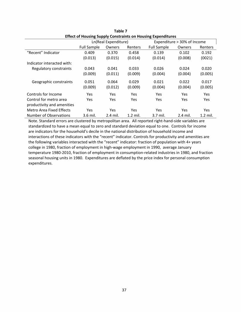
We also estimate the effects of housing supply constraints on housing expenditures. These 

expenditures combine effects on housing costs with consumption and location decisions. We 

find that both constraints raise housing expenditures by a bit more than implied by the model, 

although still by less than the estimated effects on house prices.  

 

Broadly speaking, our empirical results accord with the predictions of the model, in that we 

find much smaller effects of regulation on rent than on house prices and can reject large 

household adjustments along most dimensions.  One interesting exception is the effects of 

geographic constraints, where the model predicts that most households remain in the city and 

occupy houses on much smaller lots, while spending no more on housing.  In contrast, in the 

data, we find that lot sizes do not shrink in response to geographic constraints but that many 

households migrate out of the city.  Moreover, the data suggest that household expenditures 

rise somewhat in more geographically constrained areas.  These results are consistent with the 

possibility that minimum lot sizes and other regulatory constraints prevent households from 

adjusting their housing consumption as much as they would prefer, pointing to a potentially 

important interaction between geographic and regulatory constraints.  Banzhaf and Mangum 

(2019) also find evidence that structural and regulatory constraints create frictions in housing 

consumption. 

 

One issue that our model does not address is location choice within a metro area. We might 

observe little adjustment along the dimensions of housing consumption or metro‐level sorting 

because households instead offset higher housing costs by choosing to live in neighborhoods 

    

4  

with relatively low land prices, such as those with long commutes. We look for evidence of this 

possibility by examining housing construction by Census tract from 1980 to 2016. We measure 

neighborhood amenities with distance to the metro central business district, average commute 

time, school quality and crime. We find no evidence that supply constraints have increased the 

housing stock in relatively less‐desirable neighborhoods. Therefore, it seems unlikely that 

household location choice within a metro is sufficient to obscure or offset large effects of 

supply constraints on the price of housing services. 

 

In summary, we find that the effects of supply constraints on the price and quantity of 

housing services are substantially smaller than their effects on house prices. Because it is 

housing services, and not homeownership, that matters for welfare, our results suggest that 

the housing consumption and affordability distortions from supply constraints are much smaller 

than the effect on prices would suggest.  

 

2. Model 

2.1. Environment and equilibrium 

There are two cities,   (for “regulated”) and   (for “free”). Time runs continuously from0. The economy consists of  households, each living in one of these two cities. The utility of 

household  is 

log , , , , , , 

where   is the time the household is born,  is the discount rate, ,  is its taste for city , ,  is 

non‐housing consumption, and ,  is housing consumption. Flow utility from non‐housing and 

housing consumption is Cobb‐Douglas: , , , , , , where  ∈ 0,1 . The household 

receives income  that is constant over time. The distribution of income across households has 

a probability density function . 

Households differ in their city tastes: 

,

,

, 

where  ,  and  ,  vary as independent standard extreme value distributions and 0.3 We 

assume that city tastes are independent from household income. 

Each household is part of a “dynasty,” a collection of households with identical income and 

city tastes. At a given time, the dynasties contain the same number of households, and the 

                                                            3 McFadden (1973) demonstrates the useful properties of extreme value distributions in the context of logit 

choice models. 

    

5  

number of households grows at a rate . Each dynasty chooses cities and consumption levels 

for its households to maximize the sum of their utility. The dynasty can borrow against the 

future income of its households at a constant rate , yielding the budget constraint  

, , , ,

∈ ∈

, 

where ,  is the rental price of  units of housing in city  at time , and the price of non‐housing consumption equals one. Although an artificial modeling device, the dynasty 

represents bequests between generations and preserves symmetry in the model between 

households who arrive at different times. 

Competitive developers supply housing in each city using two inputs: land, , and tradeable capital, . Epple, Gordon, and Sieg (2010), Ahlfeldt and McMillen (2014), and Combes, 

Duranton, and Gobillon (2016) find that a constant returns to scale, Cobb‐Douglas function of 

these two inputs approximates the production process for housing very well. Thus, we assume 

the following production function in our model: 

, , 

where0 1. To abstract from issues of durability, we allow developers to supply housing 

services in frictionless spot markets. The marginal flow cost of structure is  and the marginal 

flow cost of land assembly is . These costs are identical across cities and constant over time.  

Regulators in city  unexpectedly impose one of two restrictions on developers for all0: 

The total number of separate housing units cannot grow at a rate greater than . 

The total land used for housing cannot grow at a rate greater than . 

These rules come at the end of time 0, after developers and dynasties have made their initial 

decisions. The first restriction limits the speed at which developers may supply new housing, so 

it corresponds to delays in the permitting process as well as regulations such as permit limits 

that restrict the amount of new construction. Because each household lives in a separate 

housing unit, this regulation restricts the growth rate of the city’s population. In contrast, the 

second restriction limits the geographic expansion of the city, so it corresponds to geographic 

constraints on housing supply. It could also reflect some regulatory restrictions, such as open 

space requirements.  In city  ,the number of housing units and area of land used are 

unconstrained. 

Developers must obtain a permit to supply a housing unit at time . The endogenous permit 

price is , , with , 0 due to the absence of regulations in city . Unpermitted land 

available for development in city  trades among developers at an endogenous spot price , , 

which also equals zero in . Developer cost minimization pins down the rental price of housing: 

    

6  

, , 1 , . 

The price to buy housing outright equals the expected net present value of future rents: 

, , ′. 

Equilibrium consists of prices , , , , and ,  such that dynasties maximize utility 

subject to their beliefs and budget constraints, developers maximize profits while obeying the 

regulations in , and the housing market clears in each city. At 0, dynasties expect prices that hold in an equilibrium without any regulation, while they expect the prices that hold in the 

regulated equilibrium for 0. Appendix A.4 characterizes equilibrium at 0. 

2.2. Equilibrium effects of population constraints 

To isolate the effect of the population constraint, we set   so that the constraint 

binds, while assuming that  is sufficiently large so that the price of land in  equals zero. 

Proposition 1 describes household city choices given the path of permit prices. 

Proposition 1 (sorting). If , , , household  always lives in . If , , , 

household  lives in  only while ∗, which solves 

log ,

,

, ∗

, ∗ 

where ≡ ,∣∣ ,. 

According to the proposition, households with a greater taste for  live there until the 

permit price becomes too high. This threshold price is larger when the relative taste for  is 

greater or the household’s income is higher. Because the threshold rises in income, regulation 

skews the city income distribution to the right, inducing outmigration of poorer households. 

In equilibrium, the number of households choosing  must equal the maximal number that 

city  allows. To calculate the former, we compute the number of households at  whose relative taste for  exceeds the right side of the equation in Proposition 1 for ∗ . The 

latter comes from growing the initial population (appearing in Appendix A.2) by . Equating 

these gives 

exp ,

,

,

. 

This equation pins down , . In particular, ,  must strictly increase over time, reflecting the 

increasingly binding nature of the population constraint. Proposition 2 proves this result, but it 

    

7  

is easy to see because the left side decreases in  while the right side decreases in , . The 

increasing nature of the permit price means that regulation increases prices more than rents: 

Proposition 2 (prices versus rents). The permit price, , , strictly increases in . The effect of regulation on rents,  

,

,1 ,

1 

is therefore less than the effect of regulation on ownership prices, 

,

,1

,

1 

for all positive  and . 

Each household living in  subtracts some constant amount from its flow income to pay the 

permit price. This deduction corresponds to  in Proposition 1. The remaining income goes 

toward structure, lot, and non‐housing consumption. Due to Cobb‐Douglas preferences and 

production, the shares of remaining income going to these purposes are , 1 , and1, respecitively. Proposition 3 formalizes this argument. 

Proposition 3 (housing characteristics). Structure and lot sizes for household  in  are 

∗ ∗ ∗ 1 ∗ . 

Both ∗ ∣  and ∗ ∣∣  strictly increase in  at each . 

Proposition 3 establishes two offsetting effects of regulation on housing characteristics. 

Holding income constant, regulation unambiguously decreases structure and lot sizes by 

increasing ∗ . This mechanism is an income effect: the permit price makes households 

poorer, leading them to consume less housing. Offsetting the income effect is a sorting effect. 

Holding the characteristics conditional on income constant, the sorting of poor households out 

of city  drives up average characteristics in  because these characteristics increase in income. 

The net effect of regulation on the average structure and lot size in city  is ambiguous. 

2.3. Equilibrium effects of geographic constraints 

To isolate the effect of geographic constraints, we set   so that the constraint binds, 

while assuming that  is sufficiently large so that the permit price in  equals zero. 

Proposition 4 describes household city choices given the path of permit prices. 

Proposition 4 (sorting). Household  lives in  only if 

log ,

,1 log 1 ,

 

    

8  

and lives in  when this inequality does not hold. 

As with population constraints, geographic constraints lead some households with a higher 

taste for  to live in . But different from the population constraints, this outmigration is 

independent of household income because of Cobb‐Douglas preferences and production. The 

housing characteristics for households in  clarify this point: 

Proposition 5 (housing characteristics). Structure and lot sizes for household  in  are 

∗ ∗ 1 , . 

By driving up the marginal cost of assembled land ( , ), geographic constraints lead to 

smaller lot sizes. The proportional decrease in lot size is the same for all income groups, and 

coincides with the term on the right side of the inequality in Proposition 4. This result holds 

because of Cobb‐Douglas preferences and production. Also because of Cobb‐Douglas 

preferences and production, structure size does not depend on geographic constraints. 

To solve for the equilibrium price of land, we equate the total lot sizes of households 

choosing  with the maximal size that city  allows. The former comes from Propositions 4 and 

5, while the latter comes from growing the initial city land size (appearing in Appendix A.4) 

by . This equation yields a closed‐form solution for the land price: 

, 11

1 , 

which strictly increases over time. Using this formula, we prove our final proposition: 

Proposition 6 (prices versus rents). The effect of geographic constraints on rents,  

,

,1 , , 

is less than the effect of regulation on ownership prices, 

,

,1 , ′, 

for all positive  and . 

2.4. Calibration 

We calibrate the model to quantify the effects of supply constraints on rents, housing 

expenditures, housing characteristics, and city incomes given the effect of constraints on 

    

9  

ownership prices. To perform this exercise, we need values for the various model parameters. 

The appendix gives details on how we quantitatively solve the model given parameter values. 

We use a discount rate of 0.05. We set the income distribution, , to a lognormal with 

mean $50,000 and log standard deviation 0.96, which is the mean of the standard deviations of 

positive log household income in the 1980 and 2016 U.S. Census data samples. We take0.25 from Davis and Ortalo‐Magné (2011), who find that this share of income is spent on rent in 

many cities from 1980 to 2000. We set  , which governs the distributions of preferences for R 

and F, equal to three, a value that is within the range estimated by Diamond (2016) by 

computing the elasticity of cross‐city migration with respect to changes in wages and rents. We 

set 2/3, share of construction expenditure on structure that Albouy and Ehrlich (2018) estimate. The ratio ⁄  pins down the initial relative size of city . We set it to 1 so that the 

cities have identical populations absent regulations in . The economy growth rate, , equals 

0.01, reflecting average annual population growth in the U.S. between 1980 and 2016. 

The final parameters are  and , which describe the supply constraints. We choose these 

parameters so that each constraint raises the ownership price of a constant‐quality house (at 

the median of the quality distribution at time zero) by 10% over 30 years. This magnitude is 

convenient because in our empirical estimates below, we find that a one standard deviation 

tighter constraint is associated with about 10 percent faster price growth over a roughly 30‐

year period. This methodology gives us values of 0.0092 and 0.0093. 

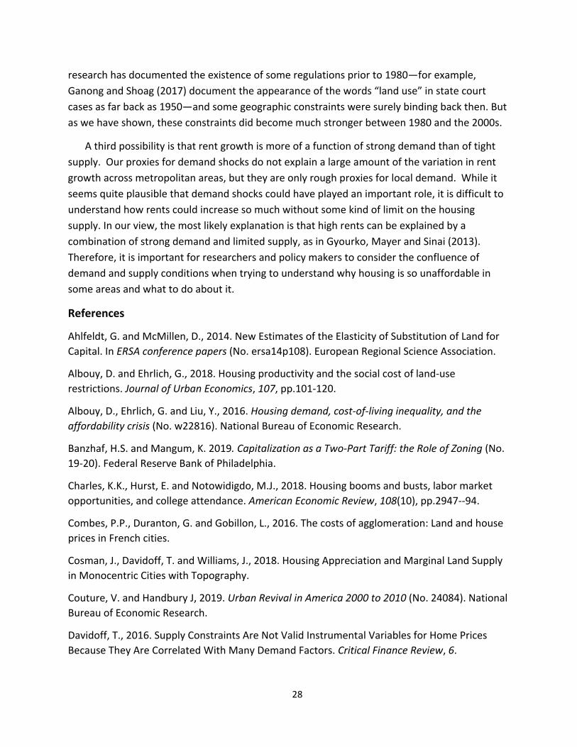
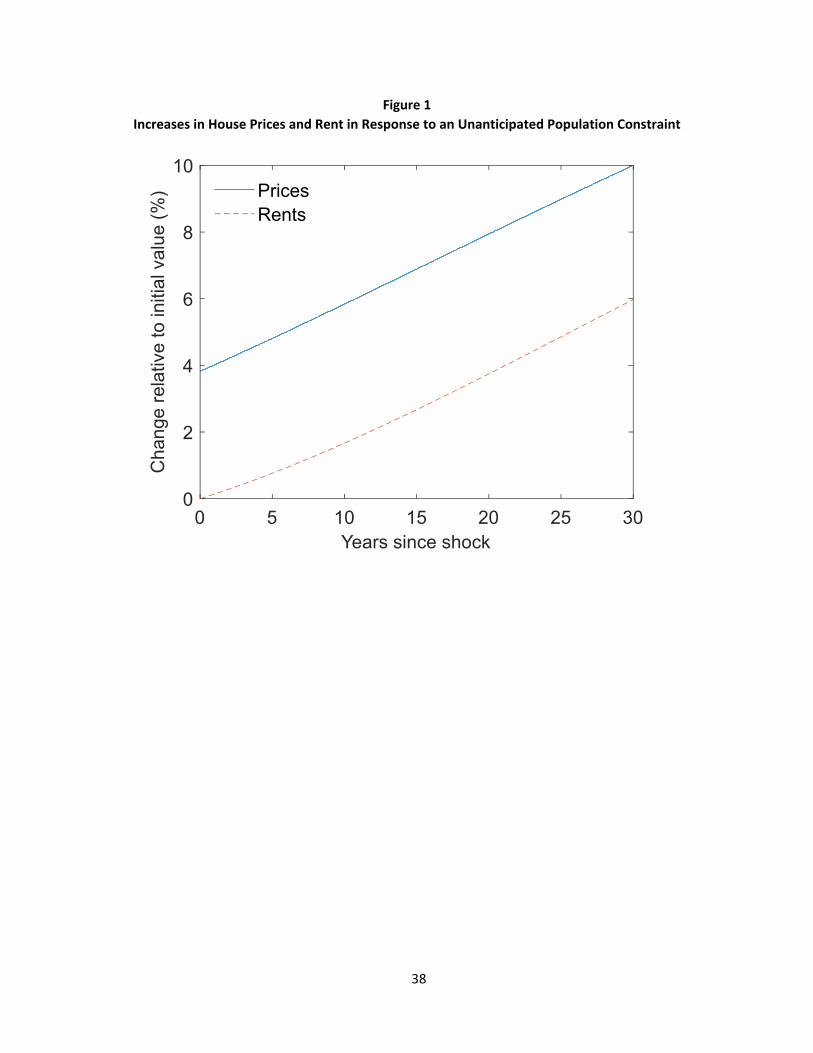
Table 1 reports changes in outcomes given this assumed price increase. The case of 

population constraints appears in column (1), while the results under land area constraints are 

in column (2). Under both supply constraints, the rent of the initial median unit rises far less 

than prices—by only about half. In other words, about half of the effect on ownership prices 

comes from anticipation of future rent increases that the supply constraints will continue to 

cause. Figure 1 illustrates this result by showing the evolution of prices and rents in response to 

the population constraint.  Initially, rent is unchanged because the population constraint only 

affects future growth.  But prices jump by about 4 percent in response to anticipated future 

rent increases.  Over time, prices and rents rise by similar amounts, so that the net increase in 

prices remains larger.  Although the differential between prices and rents becomes a smaller 

fraction of rent as time goes on, it is still quite substantial after 30 years.  Results are similar for 

the geographic constraint, not shown. Propositions 2 and 6 prove that the effect on rents is 

smaller than the effect on ownership prices, while Table 1 and Figure 1 illustrate that this 

difference is meaningful.   

Population constraints decrease structure and lot sizes by 1.6%, holding income constant. 

To compute this number, we calculate the drop for each household in  after 30 years and then 

take the average across households. The 1.6% decrease in structure and lot sizes is nearly an 

order of magnitude less than the increase in ownership prices and is significantly less than the 

increase in rents. Households pay for the permit price by cutting back on both housing and non‐

    

10  

housing consumption. Because housing begins as only 25% of household budgets, the permit 

price does not reduce structure and lot size very much. 

The effect of delays on the average housing characteristics in the city is not as negative as 

the effect given household income, as lower‐income households are more likely to move out of 

city  (as predicted by Proposition 3). However, the effect is still negative and is close to zero. 

Consistent with sorting by income, population constraints raise the median income in the city 

by 3.0%. Finally, population constraints raise the expenditures for the average household 

remaining in  by 2.7%.  This increase is smaller than the increase in quality‐adjusted rent 

because households reduce their consumption of structure and land. 

Geographic constraints reduce lot sizes by 18.8%, which is nearly double the effect on 

house prices. This type of constraint as no effect on structure size, housing expenditure shares, 

or median city income. The lack of adjustment along these dimensions results from Cobb‐

Douglas preferences and housing production, through which an increase in the unit price of 

land leads only to less land consumption and some out‐migration.  

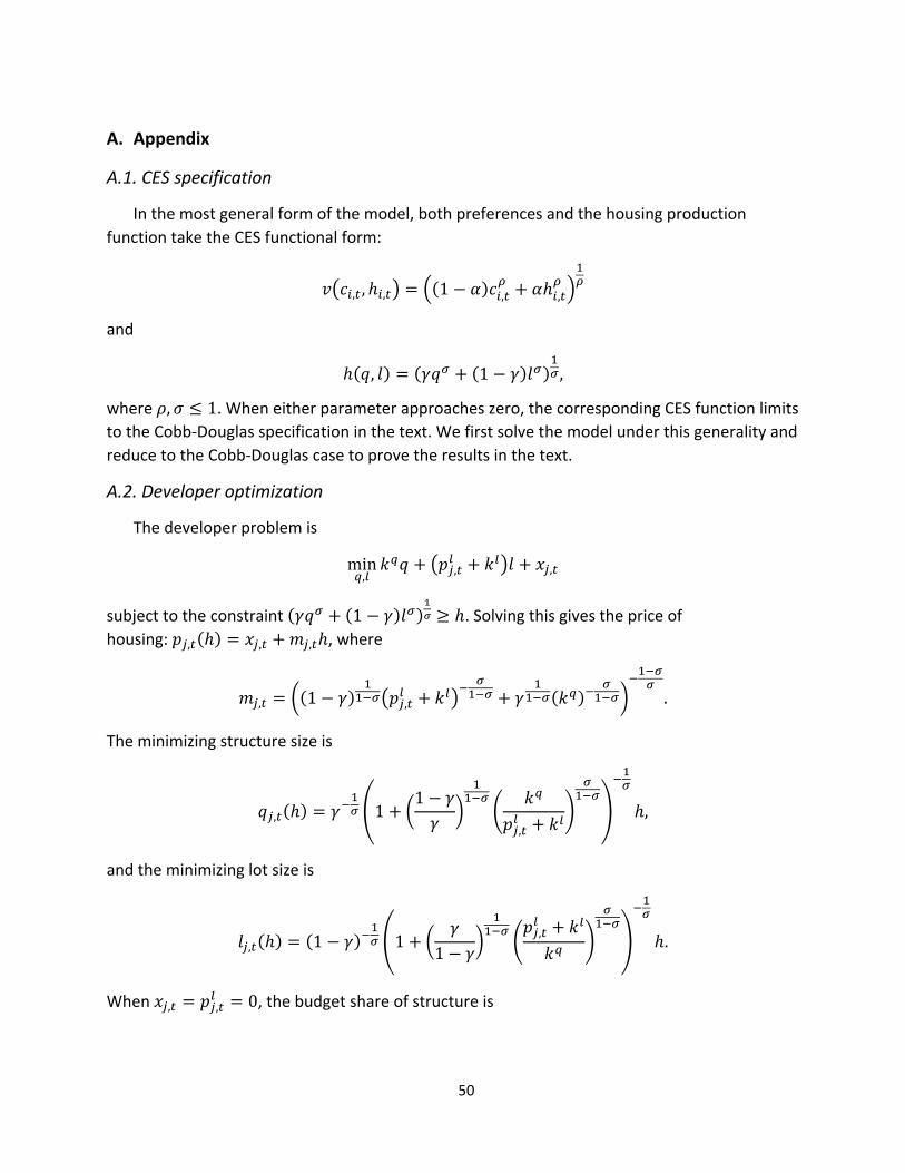
The remaining columns of Table 1 explore the case of geographic constraints while relaxing 

the Cobb‐Douglas assumptions. We instead use constant elasticity of substitution (CES) 

preferences or production, for which Cobb‐Douglas is a special case. The appendix solves this 

more general model. Column (3) reports results when preferences are CES, in which case we 

take the elasticity of substitution between housing and non‐housing consumption from Albouy, 

Ehlrich, and Liu (2016). In column (4), we also use a CES production function, taking the 

elasticity of substitution between land and structure from Albouy and Ehrlich (2018). In both 

cases, we keep the initial expenditure share on structure and housing the same as in the 

baseline calibration. 

With CES preferences, households cut lot consumption by 13.9%, still a large number but 

less extreme than before. They pay for this smaller decline in lot size by reducing non‐housing 

consumption. As a result, the expenditure share on housing rises 2.1%.  While lot sizes still fall, 

structure sizes actually increase because, with a Cobb‐Douglas production function, structure 

costs must scale with total housing costs. When the housing production function also is CES, lot 

sizes only fall by 6.6%. Housing expenditures still rise by 2.1%, but structure sizes now fall 

slightly by 1.4%. CES production makes structure and lots strong complements, meaning that 

developers cut structure sizes in response to the increase in land prices. In summary, lot sizes 

shrink markedly in these CES extensions but not by as much as in the Cobb‐Douglass case. 

Effects on other outcomes remain small. 

 

3. Empirical Strategy and Data 

    

11  

3.1. Identification 

Our goal is to estimate the effect of housing supply constraints on housing affordability, as 

measured by rent, and on households’ housing consumption and location decisions.  We 

identify these effects by comparing outcomes across metropolitan areas in the US.  Because of 

the large amount of heterogeneity in regulatory and geographic environments across locations, 

cross‐metro analysis provides a good environment in which to look for its effects.  One major 

empirical challenge, however, is that housing supply regulations correlate with many other 

aspects of local housing and labor markets that also affect the outcomes that we are interested 

in (Davidoff 2016).  Therefore, we cannot simply regress our outcomes of interest on regulatory 

variables and expect to identify a causal effect. 

We address this issue in three ways.  The first way is to focus on changes in our outcomes of 

interest over time.  This strategy allows us to abstract from other factors that might be 

correlated with regulation and housing characteristics, but are unchanging over time.   For 

example, structure costs might vary across locations due to the availability of various types of 

construction materials.  Or preferences over housing versus other consumption might differ 

across locations.  The second way is to control for some time‐varying factors that might be 

correlated with regulation and housing outcomes—specifically variables that reflect local 

productivity growth and amenities.  The third way is to exclude metropolitan areas with low 

housing demand from our analysis, since housing markets in these areas likely differ from other 

areas in many unobservable ways that might be correlated with our outcomes of interest.  We 

write this identification strategy as: 

, 

where  is an outcome for household  in metro  at time ,  is a metro dummy,  is a 

time dummy,  is a vector of supply constraints in metro  at time , and  is a vector of 

controls. The coefficient of interest is . 

We do not have detailed data on how supply constraints have changed over time, so we 

cannot include these changes directly in our analysis.  Instead, we assume that these 

constraints have become more binding over the past four decades.  Motivated by this 

assumption, we compare observations from 1980 ( ) to observations in the 2010s (

). Given that , 0, we may rewrite the above specification as 

1 1 , 

where   equals the average value of the supply constraint and   equals the average values 

of the controls that we use to proxy for changes in local productivity and amenities. 

    

12  

Prior research examining the evolution of housing supply regulation in specific locations 

supports the assumption that supply constraints were not very important before 1980.  In a 

sample of 402 California cities, Jackson (2016) finds that most regulations that affect the size, 

location, or density of the housing stock were established after 1985.  In a study of 

communities in the Greater Boston area, Glaeser and Ward (2009) show that most cluster 

zoning regulations, wetlands bylaws, and septic system requirements were adopted in the 

1980s or later.  While subdivision requirements were more common than these other 

regulations in the 1970s, nearly half of the communities in their sample adopted subdivision 

requirements after 1980.  Massachusetts and California are well‐known to be among the more 

highly‐regulated states, so it is unlikely that housing supply regulations became widespread in 

other states before reaching these two states.  Ganong and Shoag (2017) report a steady 

increase in the fraction of state appellate court cases that contain the phrase “land use” from 

1980 to 2010—from about 0.25 percent in 1980 to 0.4 percent in 2010.4 

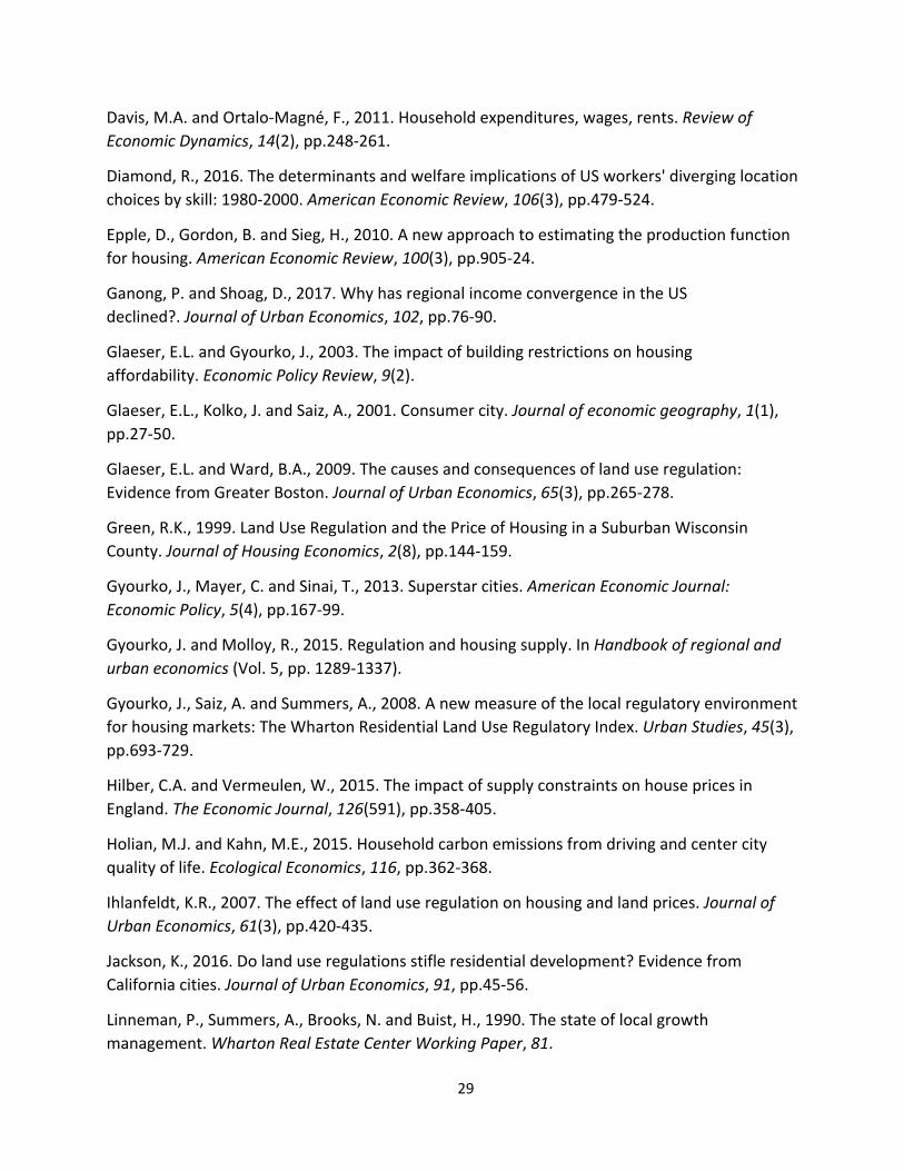
We can look for further evidence of changes in the regulatory environment using data from 

two surveys conducted by researchers at the Wharton School of Business.  Both surveys asked 

local government officials about the length of time typically required for a building permit 

application to be approved.  The first survey was conducted in the 1980s (Linneman, Summers, 

Brooks and Buist 1990), and the second survey was conducted in 2006 (Gyourko, Saiz and 

Summers 2008).  Table 2 reports the approval times for the 60 metropolitan areas that were 

covered in both surveys. In the 1980s, median application time for a single‐family construction 

permit was 2 months, and the 90th percentile was 3 months.  By contrast, in 2006 median 

application times ranged between 6 and 8 months, depending on the type of permit.  And 90 

percent of metropolitan areas had permit approval times greater than 3 months.  The median 

increase in approval time across metro areas was in the range between 4 and 6 months.   And 

because approval times were so low in all metro areas in the 1980s, the locations with the 

longest approval times in the 2006 are also the ones that experienced the largest increases in 

approval time. 

The topography of the land changes quite slowly over time, so one might question how 

geographic constraints might become more binding over time.  Cosman, Davidoff and Williams 

(2018) develop a model to show that in an expanding city, it is the marginal supply of land at 

the edge of the city that affects prices, not the average supply of land throughout the city.  They 

argue that the marginal supply of land at the edge of the city does not decrease over time since 

the boundary of the city shifts out.  However, in some metropolitan areas like San Francisco the 

terrain becomes more mountainous toward the edge of the metro, so the constraints become 

more binding as the metro grows toward these constraints.  Moreover, infill development is 

                                                            4 The incidence of court cases related to land use began increasing in 1960, illustrating that some regulations 

were binding in some locations prior to 1980. 

    

13  

fairly common in many metropolitan areas, and as housing demand in a city increases and more 

homes get built, less land will be available in the interior of the city for further new 

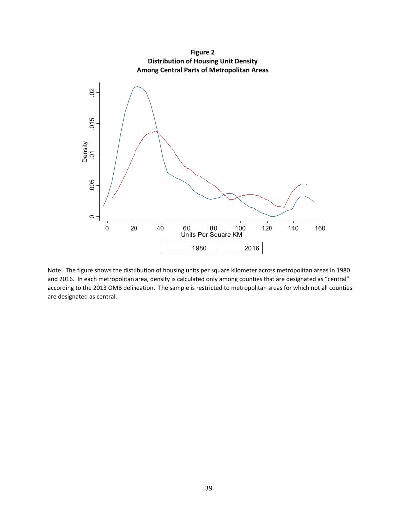
construction.  To demonstrate the importance of infill development, Figure 2 shows how 

housing unit density in the central parts of metropolitan areas has changed from 1980 to 2016.5  

In 1980, about two‐thirds of metropolitan areas had an average density of less than 40 units 

per square kilometer in their central counties.  By 2016, only about one‐third of metros had an 

average density this low in their central counties.  Thus, there has been a substantial amount of 

residential construction in the interior of metropolitan areas, and so we think it is reasonable to 

assume that the supply of land throughout the city matters for determining the supply of 

housing. 

Our specification identifies   when | , 0. The controls must explain all of 

the changes in the outcomes over time within metros that correlate with the growth in supply 

constraints but are not caused by the supply constraints. The controls that we think are most 

important are proxies for productivity growth and changes in the value of local amenities. 

Metros that have witnessed growth in regulatory constraints have also seen higher productivity 

growth (Saiz, 2010; Davidoff 2016), which could increase household income and alter 

equilibrium housing characteristics. Similarly, many supply‐constrained metros are in locales 

commonly viewed as having desirable amenities.  The amenity premium may have increased 

over time, perhaps because the aggregate population has become wealthier.  We will discuss 

the variables that we use as proxies for changes in local productivity and amenities below. 

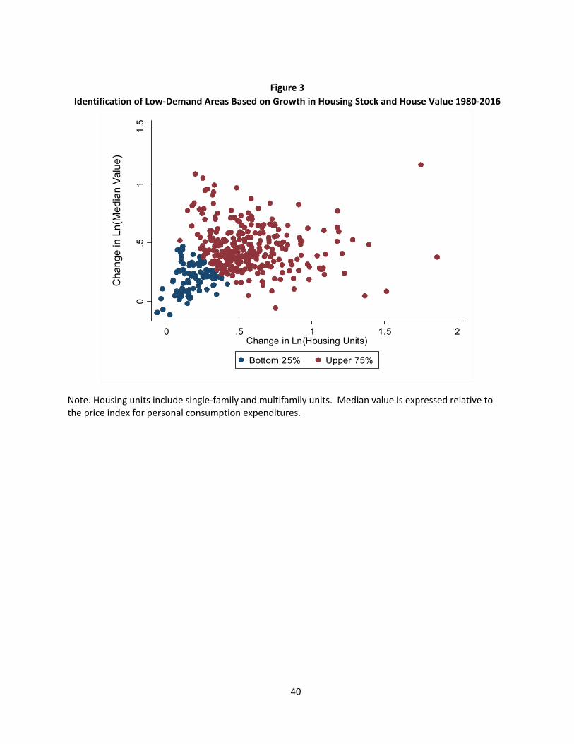
Our third attempt to address the endogeneity of supply constraints is to exclude low‐

demand metropolitan areas from our analysis.  These areas have quite different housing market 

dynamics from growing areas, and they are different along many unobservable dimensions as 

well as observable dimensions.  Moreover, it is unlikely that supply constraints would bind in 

these areas.  Following Gyourko, Mayer and Sinai (2013) and Charles, Hurst, and Notowidigdo 

(2018), we calculate housing demand in each metro area as the sum of the percent change in 

the number of housing units and the percent change in house value from 1980 to 2016.6  Low‐

demand areas are those in the bottom quartile of the demand distribution, and are dropped 

from our analysis.  Figure 3 plots growth in the housing stock against growth in house values 

over this period and shows the dropped metro areas in blue. 

3.2. Data on supply constraints 

                                                            5 In the 2013 designation of which counties are in metropolitan areas, the Census Bureau identifies some 

counties in each metropolitan area as “central”.  We use this indicator to define central counties and limit our analysis to metropolitan areas for which not all counties are designated as central.   

6 Data are from the 1980 Census and 2016 American Community Survey.  We take published data by county and aggregate to the 2013 metro area definitions.  House value is calculated as the housing unit‐weighted average of county median values. 

    

14  

As a proxy for constraints that reduce the future growth rate of the housing stock, we use 

an index of the strictness of housing supply regulation based on the Wharton Residential Land 

Use Regulation survey (Gyourko, Saiz and Summers 2008).  In 2006, these researchers sent a 

survey to local government officials asking a range of questions about the types of residential 

land use regulation currently used and the political process through which land use regulations 

are formed.  They combine the answers to the questions into a single index of regulatory 

stringency which is available for 259 metropolitan areas. The index is normalized to have a 

mean of zero and a standard deviation equal to one.   

As a proxy for the supply of buildable land, we use data on geographic constraints.7  

Specifically, we use the data underlying Saiz’s (2010) estimates of the fraction of land that is 

unavailable for construction because it is on a steep slope or covered by water.8  This measure 

is also normalized to have a mean of zero and a standard deviation equal to one.  The 

regulation index and the index of geographic constraints constitute our two components of  . 

Not only are the estimated effects of geographic constraints interesting in their own right, 

but they are helpful to include in our analysis for better identification of the effects of 

regulation.  For example, Saiz (2010) shows that stricter housing supply regulations developed 

in areas with tighter geographic constraints.  Also, the mountains and bodies of water that 

make it more difficult to build are frequently seen as positive amenities, and an increase in the 

desirability of these amenities from the 1970s to the 2000s may have raised housing demand in 

areas with tight geographic constraints (Cosman, Davidoff and Williams 2018). Consequently, 

while the identification strategy is not as clear for the geographic constraints as it is for the 

regulatory constraints, we would want to include the geographic constraints anyway in order to 

more clearly identify the effect of regulation. 

3.3. Data on outcomes 

To examine affordability directly, we use data on rent and property value from the 1980 

Census and the 2012‐2016 American Community Survey (ACS).9  Specifically, we use the 

variable reflecting gross rent, which adds utilities costs to contract rent in cases when utilities 

                                                            7 One of the components of the regulation index is related to open space requirements, which one could view 

as a constraint on the supply of buildable land.  However, it is so strongly correlated with other components of the index that we do not believe it is possible to use it to identify the effects of land supply separately from other types of regulation. 

8 Saiz (2010) calculates these constraints for a radius of 50 kilometers around the center of each of 100 metropolitan areas.  We alter this calculation slightly by calculating the fraction of unavailable land for all of the land area in the metropolitan area, which allows us to compute geographic constraints for a larger set of metropolitan areas. 

9 Data obtained from the IPUMS USA (Ruggles et al. 2019).  To harmonize the definition of metropolitan area over these two samples, we construct a cross‐walk from the four‐digit metropolitan delineations used in 1980 (IPUMS variable METAREA) to the 2013 OMB delineations (IPUMS variable MET2013). 

    

15  

are not already included, to ensure comparability across units.  We assign a value of  to 

all responses in the 1980 Census and a value of  to all responses in the 2012‐2016 ACS.  

Our housing consumption outcomes come from two different sources of property‐level 

data.  The first is a 2014 cross‐section of tax assessor data collected by CoreLogic.  Tax assessors 

record a variety of property characteristics for the purpose of assessing property values and 

determining property taxes.  This dataset covers the vast majority of single‐family housing in 

the US, although important variables are missing or have unreasonable values in a non‐trivial 

number of cases.10  Importantly for our purposes, we can obtain information on the square 

footage of the housing unit, the square footage of the lot, and the construction year of the 

property. We use the natural logarithm of unit size and lot size as outcomes. We assign a value 

of  to any house built between 1960 and 1980 and a value of  to any house 

built on or after 2000.11  We drop units built before 1960 or between 1980 and 2000 from the 

analysis. 

While the tax assessor data provide the most comprehensive data on housing unit 

characteristics with coverage across all metropolitan areas in the US, two drawbacks of the data 

are worth discussing.  The first is that we only observe housing characteristics as they were in 

2014.  To the extent that some homes built in the 1960s and 1970s have been renovated, their 

2014 characteristics do not reflect the characteristics at the time the homes were built.  The 

second drawback is that the data only cover single‐family homes. To the extent that household 

demand can switch between single‐family and multifamily units in response to price changes, 

these data may not capture all of the effects we are interested in.   

To address these drawbacks, we return to the Census/ACS data and examine two additional 

outcomes.  The first outcome is an indicator for whether a property is a single‐family structure.  

We interpret this outcome as a measure of lot size, since single‐family homes are associated 

with much bigger lots (per housing unit) than multifamily homes.  That said, single‐family 

homes tend to be larger than multifamily units, so the single‐family indicator should also be 

correlated with housing unit size.12  The Census and ACS data do not have good measures of the 

size of the housing unit or lot.13  The second outcome that we examine is the number of adults 

                                                            10 For computational reasons, we use a 25 percent random sample with 19 million usable observations.  Thus 

the full dataset, with the same restrictions, would have about 75 million observations. 11 To prevent our results from being driven by outliers with very high values, we drop housing units larger than 

10,000 square feet and units with lots larger than 175,000 square feet (about 4 acres).  We also drop units with extremely small recorded lots (less than 2000 square feet) and units with very high ratios of floor area to lot size. 

12 In the 2015 American Housing Survey, the median size of single‐family detached homes was 1805 square feet, while the median size of units in structures with 2 to 4 units was 900 square feet and the median size of units in structures with 50 or more units was 800 square feet.  Table created at the AHS website: https://www.census.gov/programs‐surveys/ahs/data/interactive/ahstablecreator.html. 

13 The datasets do record the number of rooms and number of bedrooms.  However, the tax assessor data show only a weak correlation between the number of rooms or bedrooms and the actual size of housing units, 

    

16  

per household, since people living in larger households generally consume less structure per 

person. 

In order to examine the effects of housing supply constraints on sorting across metropolitan 

areas, we aggregate the Census/ACS data to the metro level and the outcome of interest 

becomes the change in a metropolitan area characteristic from 1980 to 2012‐2016.  The first 

set of characteristics that we examine are the fraction of people in each decile of the national 

distribution of income.  Then, because annual income may not always reflect a person’s 

permanent income, we also look at two proxies for permanent income: education and 

occupation.  Specifically, we examine the fraction of the population age 25 and older with at 

least 4 years of college and the fraction of the population with a high occupation score.  The 

occupation score is created by the Census Bureau using median incomes by detailed occupation 

category using the 1950 Census. 

Finally, we examine the effects of the supply constraints on housing expenditures and the 

ratio of expenditures to household income.  Such measures are frequently used in analyses of 

housing affordability.  While our model clearly demonstrates that housing expenditures are not 

a good measure of affordability because they reflect household choices as well as the cost of 

housing services, we think these results provide a nice way to combine the effects on housing 

costs, housing consumption and location decisions. 

3.4. Data on controls 

Our empirical specification includes two proxies for productivity growth: the share of the 

population age 25 or older with at least 4 years of college in 1980, and the share of 

employment in industries that experienced fast wage growth from 1990 to 2016.  Educational 

attainment is obtained from the 1980 Census. 

To calculate the share of employment in high wage‐growth industries, we calculate wage 

growth from 1990 to 2016 by industry using the annual files of the Quarterly Census of 

Employment and Wages (QCEW).  Wages are defined as total annual wages divided by total 

annual employment.  We define industries using 3‐digit NAICS codes, which gives us 96 industry 

categories.  Although we would prefer to calculate wage growth from 1980 to 2016, the QCEW 

data by NAICS industry are not available prior to 1990.14  We define high wage growth 

                                                            likely because larger homes tend to have larger rooms, not just more rooms.  Another indicator that the number of rooms is a poor proxy for housing unit size is that there is little variation in the average or median number of rooms across metropolitan areas in the Census/ACS data. 

14 We could use data by 1‐digit SIC code to extend our analysis back to 1980.  However, doing so would give us only about 10 industry categories, and we think having more detailed industry definitions is more valuable than having a longer time period. 

    

17  

industries as those in the top decile of wage growth and calculate the fraction of employment 

in 1990 in those industries. 

We use three proxies for local amenities.  The first is average January temperature.  The 

value of nice weather seems to have increased since the 1970s (Glaeser and Gyourko, 2003) 

and many supply‐constrained metros are in warm locales such as California. This weather 

premium may have affected land prices, and hence housing characteristics, in ways we do not 

want to attribute to supply constraints. We obtain average January temperature by weather 

station from 1981 to 2010 from the National Oceanic and Atmospheric Administration.  We 

average the station‐level data by county, then take a weighted average across counties within 

each metropolitan area using county land area as weights. 

The second proxy for local amenities is the fraction of employment in 1980 that is related to 

the provision of local consumption amenities.  As incomes have risen over time, the value of 

consumption amenities has increased (Couture and Handbury 2019, Glaeser, Kolko and Saiz 

2001).  We define industries as providing local consumption amenities if they are in the 

following SIC‐based industries: eating and drinking places, amusement and recreation services, 

and museums and zoos. Because these industries are based on SIC codes, we are able to 

calculate their employment shares in the QCEW data as of 1980. 

The third proxy for local amenities is the share of seasonally‐vacant housing from the 1980 

Census.  Demand for seasonal housing has grown over time with the ageing of the population 

and rising incomes, and seasonal housing tends to be in high‐amenity areas that also may have 

tighter topographic or regulatory constraints.  To make coefficients comparable across 

variables, we standardize all five of the controls to have a mean equal to zero and standard 

deviation equal to one.  These measures are generally positively correlated with growth in the 

housing stock from 1980 to 2016, consistent with the interpretation that they reflect strong 

housing demand (see Appendix Table 1).15 

Beyond the metro‐level controls for productivity and amenities, two other sets of controls 

bear mentioning.  For the specifications with rent and house value as the dependent variable, 

we control for all available property characteristics: building age, number of rooms, number of 

bedrooms and a single‐family indicator.16  The reason for these controls is because we are 

interested in constant‐quality rent and price effects.   

                                                            15 The fraction of highly‐educated adults is roughly uncorrelated with housing stock growth in the regressions 

shown in the Appendix.  However, we prefer to include this variable as a control because it is a common proxy for local productivity. 

16 Specifically, we include indicators for decade of year built, indicators for each value of number of bedrooms, and indicators for each value of number of rooms. 

    

18  

For specifications that examine housing characteristics as an outcome, we need to control 

for household income.  As shown by the model, doing so accounts for the effects of supply 

constraints on sorting across metros, isolating the effects on the choices made by households of 

a given income level.  The specific method of controlling for household income depends on the 

outcome data we are using.  When we are using the Census and ACS data, we include indicators 

for the household’s decile in the national distribution of household income.  We allow for this 

flexible specification of income in case housing consumption choices are not a linear function of 

income.  When we are using the tax assessor data, we also control for decile in the national 

income distribution, but the income measure is median Census tract income from the 2011‐

2015 American Community Survey (ACS).  Because we do not have tract income for 1980, we 

include interactions of the decile indicators with the time period indicator.17     

 

4. Results 

4.1. Effects on Housing Affordability 

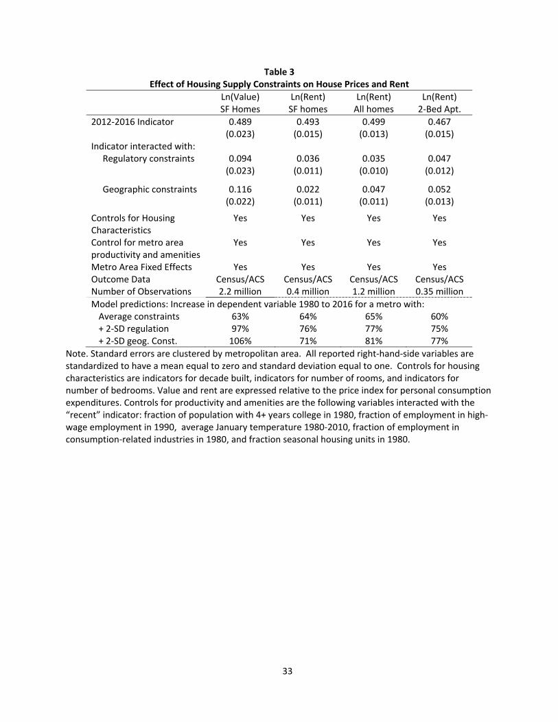
We start by examining the effects of housing supply constraints on real house prices and 

rents.    The first column of Table 3 reports the estimated effects of our two supply constraints 

on single‐family house values in the Census/ACS data.  A metropolitan area with regulations 

that are one standard deviation tighter than average experienced a 0.094 log point (about 10 

percent) stronger house price appreciation over our sample period.  The estimated effect of 

geographic constraints is slightly larger.  Results are similar when we measure house prices 

using a repeat‐sales price index instead of owner‐reported house values in the Census/ACS (not 

shown). 

Effects of this magnitude are considerable.  To illustrate, we convert the coefficient 

estimates to growth rates for a metropolitan area with average supply constraints (using the 

regression constant) and for a highly‐regulated metropolitan area that has a constraint two 

standard deviations above the mean.  The bottom rows of the table show that house prices 

doubled (in real terms) in a highly regulated area, whereas they rose by 63 percent in a 

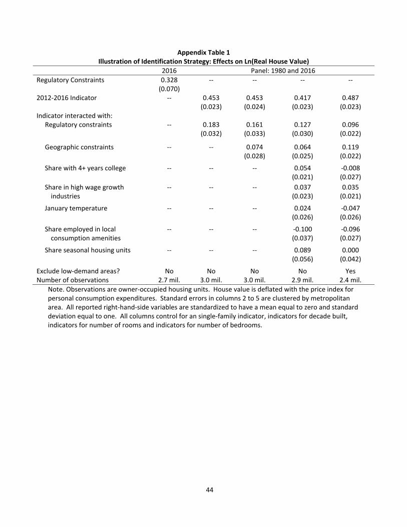
metropolitan area with average regulation.  Even so, it is worth noting that our identification 

strategy leads us to estimate much smaller effects than one would expect from the raw 

correlations in the data.  For example, the estimated effect of regulation would be more than 

three times as large if we were to estimate it from the cross section of metropolitan areas in 

2016 with no other controls.  Estimation based on changes in house values from 1980 to 2016 

reduces the estimated effect by about half, and the estimated effect is reduced further by 

                                                            17 For a future draft, we might be able to obtain these estimates. 

    

19  

controlling for geographic constraints, controlling for productivity and amenities, and excluding 

low‐demand areas (see Appendix Table 1). 

The second column of Table 3 reports the estimated effects of supply constraints on the 

rent of single‐family homes.  We start with single‐family rentals because these structures are 

more similar to the structures used to estimate the effects on house prices.  For each supply 

constraint, the estimated effect on rent growth is less than half of the estimated effect on 

house price growth.  The third column of Table 3 reports the estimated effects on rent in a 

sample of all rental homes, which is a more comprehensive sample of rental units.  Still the 

estimated effects on rent are less than half as large as the estimated effect on prices.  These 

results are especially striking because the average increase in real rent over this period was 

about the same as the average increase in real house prices, as shown by the coefficients on 

the 2012‐2016 indicators.  Thus, consistent with the model, we find that supply constraints 

increase rent by much less than house prices.   

Not only are the estimated effects on rent small relative to the effect on prices, they are 

small in absolute magnitude.  For example, based on column 3 a metro area with regulation 2 

standard deviations tighter than average experienced only 0.07 log point larger rent increases 

from 1980 to 2016, which works out to less than ¼ percentage point faster growth per year.  

The fourth column of Table 3 reports the estimated effects of supply constraints on the rent of 

2‐bedroom apartments, which is a structure type commonly occupied by low‐income 

households.  While the magnitudes are a bit larger for this sample than for the sample of all 

rental units, they still suggest that metropolitan areas with 2 standard deviation tighter 

regulatory constraints than average experienced only a 0.094 log point larger increase in real 

rent growth over this 36 year period (about ¼ percentage point faster growth per year).  Thus, 

we find that supply constraints have only reduced housing affordability by a modest amount 

over this period. 

One immediate question that may come to mind is whether our measures of supply 

constraints may be poor proxies for true supply constraints, which would cause us to 

underestimate the effects on prices and rent.  While there is surely some degree of 

measurement error in these measures, they are commonly‐used in academic research and have 

been shown to be correlated with the elasticity of housing supply (Saiz 2010).18  One way to 

assess our estimated effects is to compare them to other research that identifies these effects 

using other data and other identification strategies.  Few academic studies have estimated 

causal effects of supply constraints on house prices owing to the difficulties with measurement 

and endogeneity (Gyourko and Molloy 2015).  The most comparable analysis we have found is 

                                                            18 To date, the papers introducing the regulatory index and the geographic constraint measure have been 

cited in 170 and 347 published journal articles, respectively. 

    

20  

Hilber and Vermeulen (2016), who examine the effects of supply constraints on house prices 

across local planning authorities in England, instrumenting for regulation using a policy reform 

and spatial variation in Labour party votes.  They find that a one standard deviation decrease in 

regulation is associated with 14 percentage point lower cumulative house price growth from 

1974 to 2008, a result that is in line with our estimated effects on house price growth in the US. 

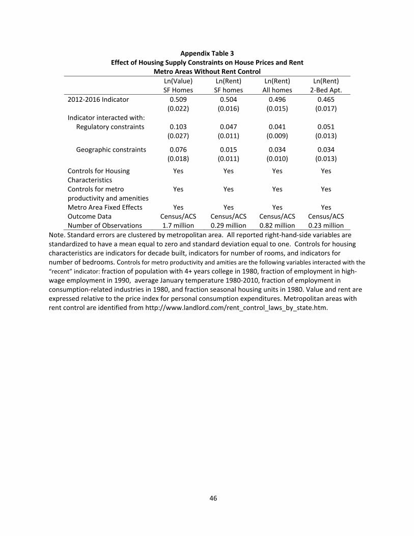
Another question that may come to mind is whether rent control might prevent rents from 

responding to supply constraints as much as prices.  We obtain a list of jurisdictions with rent 

control in 2014 from Landlord.com19 and drop metropolitan areas with any jurisdictions that 

have rent control.20  The estimated effects on rent in this sample remain about half of the 

estimated effect on house prices, indicating that rent control cannot explain the differential 

between these two outcomes (see Appendix Table 3).   

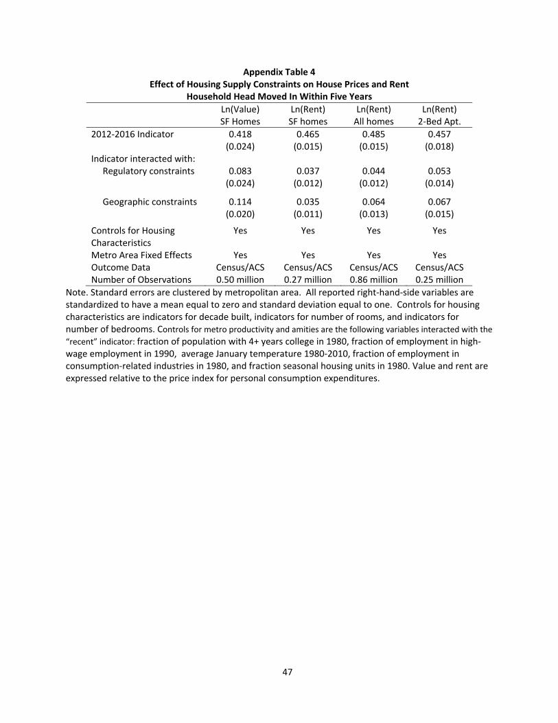
A third concern with our analysis is that the rents paid by tenants may not reflect market 

rents if the tenants have occupied the unit for a long time.  We address this issue by limiting our 

sample to households where the household head moved in within the previous 5 years.  Again, 

we find estimated effects on rent that are only half as big as the estimated effects on house 

prices (see Appendix Table 4). 

4.2. Effects on Housing Consumption 

One might be skeptical of our ability to directly examine the effects of supply constraints on 

the price of housing services because this concept is impossible to observe for owner‐occupied 

housing, which makes up roughly two thirds of all housing units.  The model illustrates how an 

increase in the price of housing services should cause households with a given income to 

reduce their consumption of housing services.  In the case of population constraints, this 

showed up as small decreases in structure size and lot size.  In the case of land area constraints, 

this showed up as a fairly sizeable decrease in lot size, with small changes in structure size 

depending on the elasticities of substitution between lots and structure and between housing 

and non‐housing consumption.  Therefore, next we examine the effects of housing supply 

constraints on direct measures of housing consumption.   

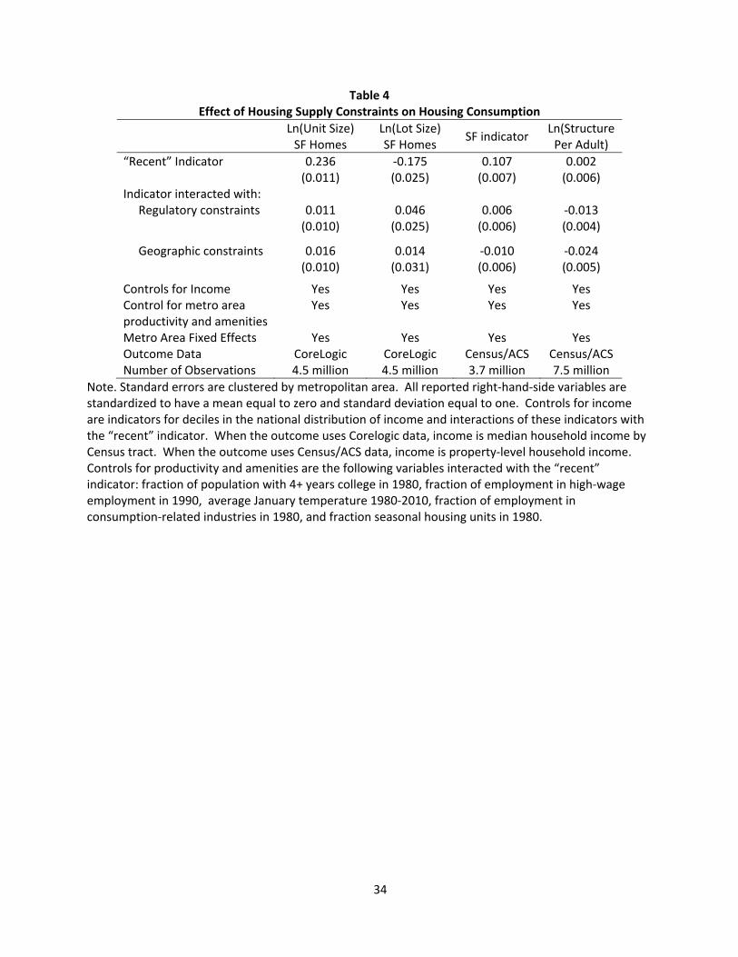
Table 4 reports the estimated effects on structure size and lot size of single‐family homes, 

and also on a single‐family indicator that signals both a larger structure and a larger lot.  The 

coefficients on regulation and geographic constraints are all small in magnitude and 

insignificantly different from zero.  In most cases, they are positive instead of negative as 

expected.  We can reject that a 1 standard deviation increase in regulatory constraints reduces 

                                                            19 http://www.landlord.com/rent_control_laws_by_state.htm. 20 There are 13 metropolitan areas with rent control according to this definition.  We treat the metro areas of 

Washington DC and Riverside CA as having rent control, even though most jurisdictions in these metros do not have rent control.  Results are similar if we treat these two metros as not having rent control. 

    

21  

structure size or lot size by more than 1½ percent, which was the magnitude of the effect 

predicted by the model.  We can also reject that a 1 standard deviation increase in geographic 

constraints reduces lot size by more than 6 percent, the smallest of the range of effects 

predicted by the model.  These results seem inconsistent with the model, and are especially 

surprising given that the estimated effects on prices and rents were in line with the model 

simulation. 

One interpretation of these empirical results is that supply constraints have a smaller effect 

on the price of housing services than predicted by the model, and also have smaller effects than 

we estimate using rent data.  Another possibility is that people generally adapt to the higher 

price of housing services in ways that are not directly captured by our model.  One such method 

of adapting could be through changes in household size.  In the model, household size is fixed 

and we can think of the predictions for housing consumption as consumption per person.  But 

in reality household sizes do vary considerably and could depend on housing costs. 

We examine empirical effects on housing consumption per person in the Census and ACS 

data.   Using individual‐level data, we estimate the effects of our two supply constraints on the 

logarithm of the inverse of the number of adults (which we define as age 18 or over) in that 

individual’s household.  This outcome can be thought of as reflecting the amount of structure 

consumed by that person.  We control for the individual’s income using indicators for their 

decile in the national income distribution, and we also control for other individual 

characteristics including age and sex. 

Table 4 shows a statistically significant negative effect of each supply constraint on 

structure per adult.  A one standard deviation greater degree of regulation is estimated to 

reduce the amount of structure per adult by about 1 percent, a magnitude that is in line with 

the model’s predicted effects on structure size.  This result suggests that instead of living in 

smaller homes, people choose to reduce their consumption of structures by living in a larger 

household.  The estimated effect of geographic constraints is also negative and a bit larger in 

magnitude, with a one standard deviation greater degree of regulation reducing structure per 

person by 2½ percent.  This result is roughly consistent with the version of the model in which 

the elasticity of substitution between lot and structure is less than one.   

Another possible explanation for these empirical estimates is that other aspects of the 

housing market or regulatory environment might prevent people from altering their housing 

consumption decisions as much as predicted by the model.  For example, regulatory constraints 

are more common in metro areas with tighter geographic constraints, and some of these 

regulations constrain the size and shape of lots.  Another factor could be the durability of 

housing, which means that the existing housing stock will slow to adapt to changes in the 

regulatory environment and changes in housing demand.  We investigate this possibility by 

    

22  

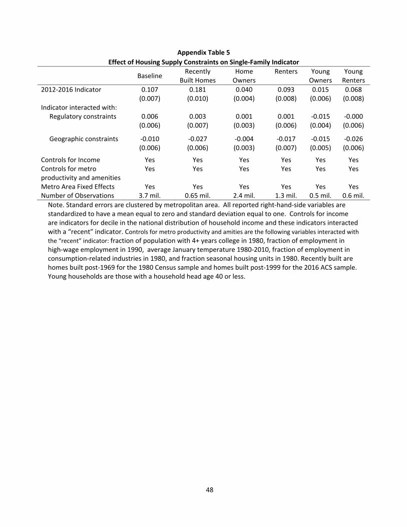
estimating the effects of supply constraints on the single‐family indicator in a sample of homes 

built within the previous 10 years.21  Although the estimated effect of regulatory constraints is 

unchanged, the estimated effect of geographic constraints becomes more negative (see 

Appendix Table 5).  Therefore, it seems plausible that other constraints may be preventing 

households from fully adapting their housing consumption choices to changes in housing 

affordability. 

A final explanation that we consider is the idea that home owners experience wealth gains 

from appreciation in house values, and they can use this additional housing wealth to increase 

their housing consumption.  In support of this possibility, the effect of geographic constraints 

on the single‐family indicator is more negative for renters than it is for home owners (see 

Appendix Table 5).  It is also more negative for young owners, who have had less time to build 

up housing equity, than it is for older owners (see Appendix Table 5).  Thus, wealth gains by 

owners of real estate may be mitigating the need to reduce housing consumption in response 

to decreases in housing affordability. 

4.3. Effects on Sorting Across Metropolitan Areas 

Next we examine the effects of housing supply constraints on sorting across metropolitan 

areas.  The model predicted that population growth would be lower in areas with greater 

supply constraints.  Prior research has generally found regulatory constraints to reduce growth 

in the housing stock (Mayer and Somerville 2000, Saks 2008, Jackson 2016).  There has been 

less research on the effects of geographic constraints on local housing or population growth, 

and the research on the effects of regulation generally does not control for geographic 

constraints.  Consequently, we start by estimating effects on the housing stock using our data 

and identification strategy. 

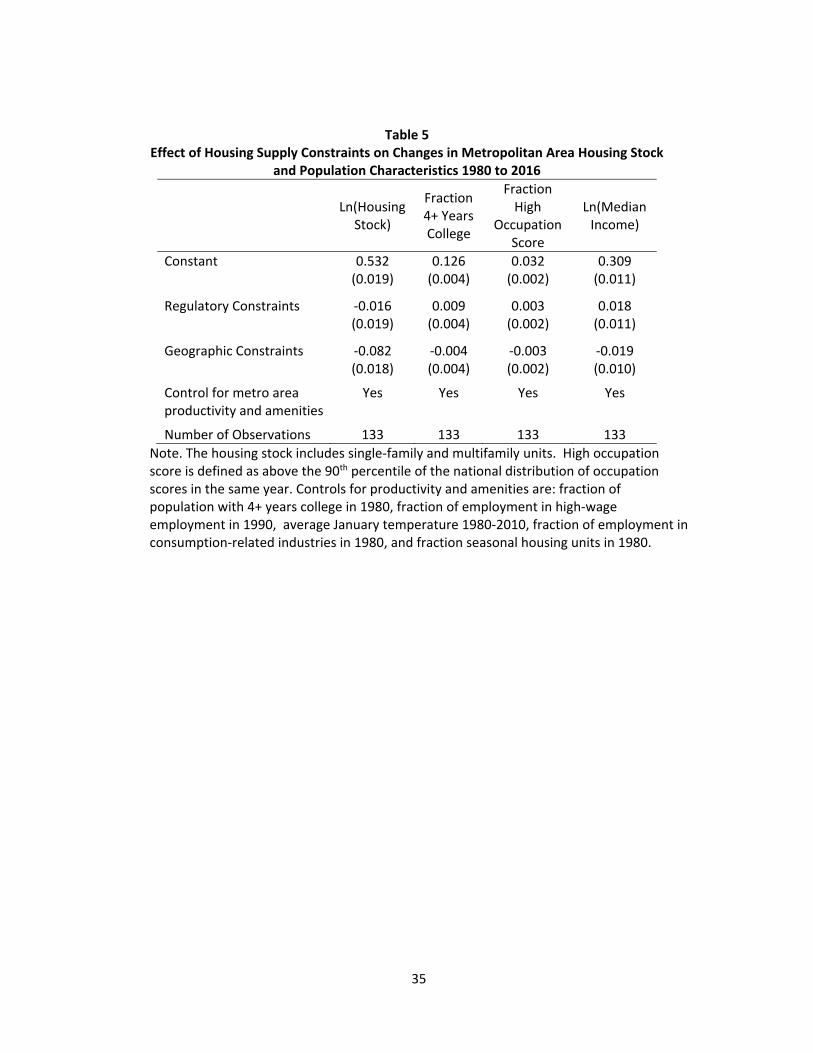
Table 5 reports the results of regressing the change in a metro’s housing stock from 1980 to 

2016 on our two supply constraints, controlling for metro area productivity and amenities.  We 

find a fairly sizeable negative effect of geographic constraints on the local housing stock—a one 

standard deviation increase in geographic constraints is associated with 8 percentage point 

lower housing stock growth.  This magnitude is larger than the model’s predicted effect of land 

constraints on population growth, which was only about 2 percent. 

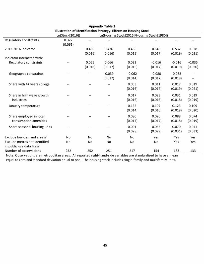
The estimated effect of regulatory constraints is also negative, but is much smaller and 

insignificantly different from zero.  One factor contributing to this result is the positive 

correlation between regulatory and geographic constraints.  If we exclude the geographic 

constraints from the regression, the estimated effect of regulatory constraints doubles in 

                                                            21 We cannot undertake a similar exercise for the unit size or lot size data because we only observe these 

homes in 2014. 

    

23  

magnitude (see Appendix Table 2).  In specifications with fewer controls, we generally find a 

positive relationship between regulation and housing stock growth (see Appendix Table 2).  This 

result illustrates the positive correlation between regulations and a variety of local factors that 

increase local housing demand, highlighting the importance of controlling for these factors 

when attempting to estimate the effect of regulations on housing outcomes.  While unobserved 

factors boosting local demand should bias our estimated effects of regulation on the housing 

stock downward, they should bias our estimated effects of regulation on house values and 

house prices upward, meaning that the true effects of regulation on housing affordability may 

be even smaller than the small effects that we estimate.     

Next, we turn to how supply constraints affect the types of people who choose to live in the 

area.  The model predicted that people with more income would be more likely to stay in areas 

with population constraints, while it predicted no effect of land supply constraints on sorting 

because we assumed that an individual’s taste for the regulated city is uncorrelated with 

income.  If instead we were to assume that income is positively correlated with changes in the 

taste for the regulated city—say because the regulated city has amenities that have become 

more valued by richer people—then we would expect land supply constraints also to cause 

sorting by income. 

We first look for evidence of income‐based sorting using data from the Census and ACS on 

income.  Specifically, we calculate the fraction of individuals in a metropolitan area that are in 

each decile of the national distribution of income.  An increase in the fraction of individuals in 

the upper deciles would be consistent with richer people sorting into that metropolitan area.  

Therefore, we regress the change in the fraction of individuals in a decile on the supply 

constraints and metro‐level controls for productivity and amenities. 

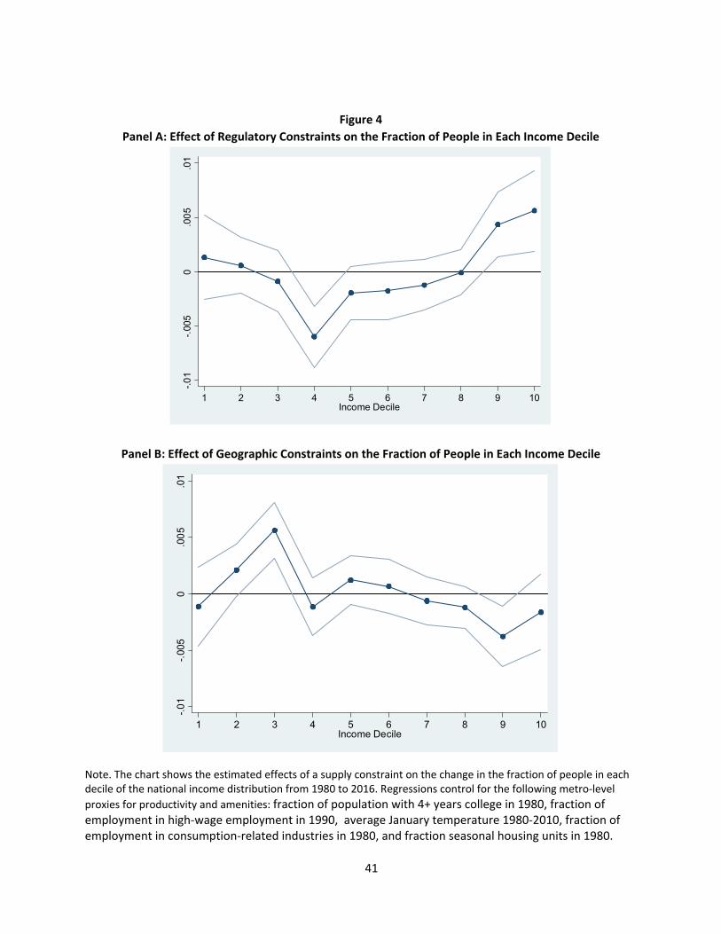
Figure 4 plots the coefficient estimates for each decile.  The results are consistent with a 

mild amount of sorting in response to regulatory constraints, as these constraints have led to 

larger shares of individuals in the top two deciles and a smaller share of individuals in lower 

deciles (although only the 4th decile is significantly different from zero).  But these effects are 

not large, as a 1 standard deviation greater regulatory constraint is associated with only about 

½ percent more of the population being in each of the top two deciles.  Similarly, we find that a 

1 standard deviation increase in regulatory constraints is associated with only a 2 percent 

increase in real median income (Table 5).  This small magnitude is consistent with the 

magnitude implied by the model.   

Figure 4 and Table 5 show no evidence of income sorting across metropolitan areas in 

response to geographic constraints, consistent with a model in which preferences for local 

amenities are uncorrelated with income. 

    

24  

Next we look at effects on sorting by education and occupation.  Regulation is associated 

with a small increase in the fraction of highly‐educated adults.  The estimated effect on the 

fraction of people in high‐income occupations is small and insignificantly different from zero.  

As with the income results, geographic constraints are unrelated to these measures of 

permanent income. 

To get a sense of the magnitudes of these effects, consider the metropolitan area of San 

Francisco, which has an appreciable amount of regulation and experienced large increases in its 

fractions of high‐income and highly‐educated residents from 1980 to 2016.  Our estimated 

coefficients imply that regulatory constraints can only explain one fifth of the increase in the 

share of residents in the top decile of the income distribution and one twentieth of the increase 

in the share of highly‐educated residents. 

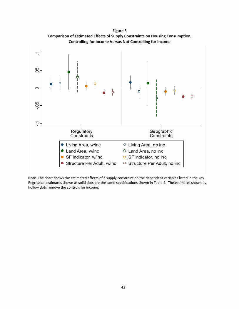
As a final method of gauging the amount of income sorting across metropolitan areas, we 

estimate effects of supply constraints on housing consumption without controlling for income.  

If supply constraints were causing a substantial amount of sorting by income, we would expect 

to find effects on average housing characteristics that are less negative than the estimated 

effects on households with a given income.  Indeed, the model simulation predicts that average 

structure size and lot size will be higher in more regulated cities, even though structure and lot 

consumption is lower at each level of income.  However, when we omit the income controls 

from each of our housing consumption regressions, in no case do the estimated effects on an 

outcome to become materially less negative (see Figure 5).  On net, our results suggest that 

much of the sorting across metropolitan areas that has occurred is due to factors other than 

constraints on the housing supply. 

 

4.4. Effects on Sorting Within Metropolitan Areas 

Another set of outcomes related to location choice that we examine is location within 

metropolitan areas.  Our model did not differentiate across locations within metropolitan 

areas, so it does not make any predictions for this type of sorting.  However, it is easy to 

imagine that households might also adjust to higher land prices by choosing to live in a 

relatively cheaper neighborhood within the metro area.   

We assess this possibility by examining whether new housing units are more likely to be 

located in less‐desirable neighborhoods in metropolitan areas with tighter housing supply 

constraints.  Neighborhood desirability is measured using four separate neighborhood 

characteristics (where neighborhoods are defined as Census tracts): distance to the CBD, 

average commute time, crime, and school quality. The center of the metropolitan area comes 

    

25  

from Holian and Kahn (2015).22  Commute time is measured in the 2011‐2015 ACS.  School 

quality data are obtained from Location Inc., and are derived by adjusting local test score data 

across states using nationwide test scores to make scores comparable across school districts.  

Crime rate data are also obtained from Location Inc., and are calculated by assigning crimes 

reported by all law enforcement agencies in the U.S. to Census tracts using a proprietary model.  

The education and crime variables range from 0 to 100, representing the percentile in the 

national distribution. 

We estimate the effect of supply constraints on location choice within the metro in the 

CoreLogic property tax data by regressing each of the four neighborhood characteristics on an 

indicator for whether the home was built post‐2000 and an interaction of this indicator with 

each supply constraint.  The regression controls for metropolitan area fixed effects, 

neighborhood income, and metro‐level productivity and amenities also interacted with the 

“post‐2000” indicator.  This specification thus reveals whether homes built post‐2000 were 

more likely to be in lower‐amenity neighborhoods if they are in more supply constrained metro 

areas, relative to the distribution of housing units in the 1960s and 1970s. 

Table 6 reports the results.  The only neighborhood amenity that is correlated with 

regulatory constraints is school quality:  More regulated metros are more likely to have newer 

housing units in neighborhoods with lower scores on the education index, relative to the 

distribution of housing units in the 1960s and 1970s.  The effect is small, however, with one 

standard deviation higher regulation reducing educational outcomes by just 0.04 standard 

deviations.  Geographic constraints have some unexpected results.  Metros with greater 

geographic constraints tend to have newer homes closer to the CBD and with lower commute 

times than less constrained metros.  And while these constraints do appear to be associated 

with a move toward higher‐crime and lower‐school quality neighborhoods, the estimated 

effects are again small.  On net, we don’t find much evidence to support the theory that supply 

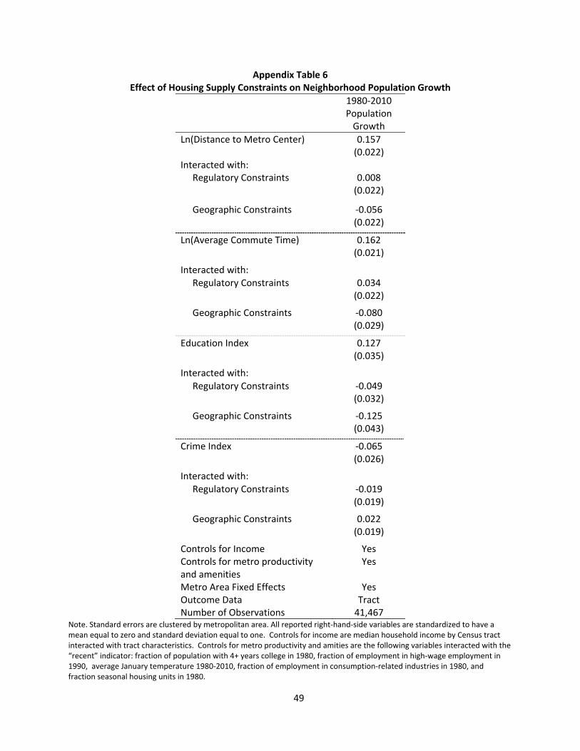
constraints have caused household to move to materially lower‐amenity neighborhoods. We 

find similar results when we look for these effects by regressing tract‐level population growth 

on the four neighborhood quality measures and interact these measures with our supply 

constraints (see Appendix Table 6). 

One important caveat to this analysis is that we cannot observe variation in supply 

constraints across neighborhoods.  If supply constraints were tighter in less‐desirable 

neighborhoods, households would be less likely to choose these neighborhoods, possibly 

offsetting the effect that we expected. On the other hand, most research has found that 

regulations are more likely to be found in wealthier areas with more desirable amenities 

                                                            22 Holian and Kahn (2015) use the location returned when entering the central city name in Google Earth, 

which they found to be qualitatively “quite reasonable in all cases”. The data are available for download at http://mattholian.blogspot.com/2013/05/central‐business‐district‐geocodes.html. 

    

26  

(Davidoff 2016).  This would create an additional mechanism by which regulation would push 

households into less desirable neighborhoods.   

4.5. Effects on Housing Expenditures 

Finally, we estimate the effects of the supply constraints on housing expenditures using the 

Census/ACS data at the household level.  Expenditures are measured as rent for renter 

households, and monthly payments for owner‐occupied households (which includes mortgage 

interest, property taxes and homeowners insurance).  Other than including data on owner 

expenditures, the main difference between this specification and the specification estimating 

effects on quality‐adjusted rent (reported in Table 3) is that we do not control for housing unit 

characteristics.  Thus we are estimating effects on rental and owner expenditures instead of 

constant‐quality rent or house values. 

Table 7 reports the coefficient estimates.  A one standard deviation tighter degree of 

regulation is associated with 4 percent higher expenditures, an effect quite similar to the 

prediction of our model.  A one standard deviation tighter degree of geographic constraint is 

associated with 5 percent higher expenditures.  The Cobb‐Douglass version of the model 

predicted that housing expenditures would not respond to a decrease in land supply, but 

allowing for an inelastic substitution between housing and non‐housing causes the model to 

predict a 2 percent increase in housing expenditures.  As we discussed above, it is possible that 

other factors, such as minimum lot sizes or density restrictions, prevent people from fully 

offsetting the effects of a tighter land supply with less land consumption, which would in turn 

lead to higher housing expenditures. 

The table also reports results where the dependent variable is an indicator for whether a 

household spends more than 30 percent of their income on housing, a common measure of 

housing “cost burden” in the affordability literature.  Both constraints increase the fraction of 

“cost burdened” households by a small amount, but even the effects of a 2 standard deviation 

tighter constraint are much smaller than the increase in “cost burdened” households over our 

sample period. 

It is possible that the housing wealth effects discussed above have allowed households to 

spend a greater fraction of their income on housing than they would have otherwise.  Table 7 

reports estimates for samples of owners and renters.  The estimated effects for owners are a 

little larger, but the only case where the difference appears material is for geographic 

constraints and ln(expenditures). 

We end this section with an examination of how the effects on housing expenditures vary 

with household income.  Most of the concerns about housing affordability are aimed at lower 

income households, so it would be helpful to know if housing supply constraints have different 

    

27  

effects for households at different points in the income distribution.  Toward this end, we 

regress ln(expenditures) and an indicator for expenditures exceeding 30 percent of income on 

our supply constraints, running separate regressions for each decile of the national income 

distribution. 

Figure 6 shows the results.  The estimated effects on expenditures are fairly similar across 

the income distribution, but are somewhat smaller for the lowest two deciles.    The effects on 

the indicator for having high housing expenditures relative to income are more hump‐shaped, 

with the largest effects of regulatory constraints in the 4th and 5th deciles and the largest effects 

of geographic constraints in the 5th and 6th deciles.  It is possible that housing programs are 

helping to reduce the effects of supply constraints on housing expenditures for low income 

households.  Meanwhile, because the effects on expenditures are fairly similar for middle‐and 

high‐income households, they are a smaller share of income as income rises. 

 

5. Conclusion 

We have shown both theoretically and empirically that housing supply constraints have a 

smaller effect on housing affordability than on the purchase price of housing.  Supply 

constraints also have only limited effects on housing consumption and location decisions. 

Our results may seem quite surprising in light of the strong cross‐sectional correlation 

between supply constraints and rents.  Indeed, even in our sample, the cross‐sectional 

correlation between supply constraints and rents is three times larger than our estimated 

causal effects.  It turns out that locations with tight supply constraints tended to have higher 

rent even back in 1980, so the changes in rent over time are not as strongly correlated with 

supply constraints as the current levels may suggest.  Controlling for measurable differences in 

demand further reduces the estimated effects of supply constraints, suggesting that supply 

constraints are also correlated with strong housing demand.   

One should not conclude from our analysis that housing affordability is not a problem in 

supply constrained metropolitan areas.  Rather, our results suggest that the supply constraints 

alone have not been the driving force behind high rents.  Why are our estimated causal effects 

so much smaller than the effects suggested by the cross‐sectional correlation between rent and 

supply constraints? One possibility is that our measures of supply constraints are not good 

proxies for true supply constraints.  But our supply constraints are more strongly correlated 

with house price growth.  Furthermore, these two constraints are the most commonly‐used 

measures in the literature.   

A second possibility is that supply constraints were at least somewhat binding even back in 

1980, in which case we have underestimated the true effects of these constraints.  Other 

    

28  

research has documented the existence of some regulations prior to 1980—for example, 

Ganong and Shoag (2017) document the appearance of the words “land use” in state court 

cases as far back as 1950—and some geographic constraints were surely binding back then. But 

as we have shown, these constraints did become much stronger between 1980 and the 2000s. 

A third possibility is that rent growth is more of a function of strong demand than of tight 

supply.  Our proxies for demand shocks do not explain a large amount of the variation in rent 

growth across metropolitan areas, but they are only rough proxies for local demand.  While it 

seems quite plausible that demand shocks could have played an important role, it is difficult to 

understand how rents could increase so much without some kind of limit on the housing 

supply. In our view, the most likely explanation is that high rents can be explained by a 

combination of strong demand and limited supply, as in Gyourko, Mayer and Sinai (2013). 

Therefore, it is important for researchers and policy makers to consider the confluence of 

demand and supply conditions when trying to understand why housing is so unaffordable in 

some areas and what to do about it.   

References 

Ahlfeldt, G. and McMillen, D., 2014. New Estimates of the Elasticity of Substitution of Land for 

Capital. In ERSA conference papers (No. ersa14p108). European Regional Science Association. 

Albouy, D. and Ehrlich, G., 2018. Housing productivity and the social cost of land‐use 

restrictions. Journal of Urban Economics, 107, pp.101‐120. 

Albouy, D., Ehrlich, G. and Liu, Y., 2016. Housing demand, cost‐of‐living inequality, and the 

affordability crisis (No. w22816). National Bureau of Economic Research. 

Banzhaf, H.S. and Mangum, K. 2019. Capitalization as a Two‐Part Tariff: the Role of Zoning (No. 

19‐20). Federal Reserve Bank of Philadelphia. 

Charles, K.K., Hurst, E. and Notowidigdo, M.J., 2018. Housing booms and busts, labor market 

opportunities, and college attendance. American Economic Review, 108(10), pp.2947‐‐94. 

Combes, P.P., Duranton, G. and Gobillon, L., 2016. The costs of agglomeration: Land and house 

prices in French cities. 

Cosman, J., Davidoff, T. and Williams, J., 2018. Housing Appreciation and Marginal Land Supply 

in Monocentric Cities with Topography. 

Couture, V. and Handbury J, 2019. Urban Revival in America 2000 to 2010 (No. 24084). National 

Bureau of Economic Research.  

Davidoff, T., 2016. Supply Constraints Are Not Valid Instrumental Variables for Home Prices 

Because They Are Correlated With Many Demand Factors. Critical Finance Review, 6. 

    

29  

Davis, M.A. and Ortalo‐Magné, F., 2011. Household expenditures, wages, rents. Review of 

Economic Dynamics, 14(2), pp.248‐261. 

Diamond, R., 2016. The determinants and welfare implications of US workers' diverging location 

choices by skill: 1980‐2000. American Economic Review, 106(3), pp.479‐524. 

Epple, D., Gordon, B. and Sieg, H., 2010. A new approach to estimating the production function 

for housing. American Economic Review, 100(3), pp.905‐24. 

Ganong, P. and Shoag, D., 2017. Why has regional income convergence in the US 

declined?. Journal of Urban Economics, 102, pp.76‐90. 

Glaeser, E.L. and Gyourko, J., 2003. The impact of building restrictions on housing 

affordability. Economic Policy Review, 9(2). 

Glaeser, E.L., Kolko, J. and Saiz, A., 2001. Consumer city. Journal of economic geography, 1(1), 

pp.27‐50. 

Glaeser, E.L. and Ward, B.A., 2009. The causes and consequences of land use regulation: 

Evidence from Greater Boston. Journal of Urban Economics, 65(3), pp.265‐278. 

Green, R.K., 1999. Land Use Regulation and the Price of Housing in a Suburban Wisconsin 

County. Journal of Housing Economics, 2(8), pp.144‐159. 

Gyourko, J., Mayer, C. and Sinai, T., 2013. Superstar cities. American Economic Journal: 

Economic Policy, 5(4), pp.167‐99. 

Gyourko, J. and Molloy, R., 2015. Regulation and housing supply. In Handbook of regional and 

urban economics (Vol. 5, pp. 1289‐1337). 

Gyourko, J., Saiz, A. and Summers, A., 2008. A new measure of the local regulatory environment 

for housing markets: The Wharton Residential Land Use Regulatory Index. Urban Studies, 45(3), 

pp.693‐729. 

Hilber, C.A. and Vermeulen, W., 2015. The impact of supply constraints on house prices in 

England. The Economic Journal, 126(591), pp.358‐405. 

Holian, M.J. and Kahn, M.E., 2015. Household carbon emissions from driving and center city 

quality of life. Ecological Economics, 116, pp.362‐368. 

Ihlanfeldt, K.R., 2007. The effect of land use regulation on housing and land prices. Journal of 

Urban Economics, 61(3), pp.420‐435. 

Jackson, K., 2016. Do land use regulations stifle residential development? Evidence from 

California cities. Journal of Urban Economics, 91, pp.45‐56. 

Linneman, P., Summers, A., Brooks, N. and Buist, H., 1990. The state of local growth 

management. Wharton Real Estate Center Working Paper, 81. 

    

30  

Malpezzi, S. and Green, R.K., 1996. What has Happened to the Bottom of the US Housing 

Market?. Urban Studies, 33(10), pp.1807‐1820. 

Mayer, C.J. and Somerville, C.T., 2000. Land use regulation and new construction. Regional 

Science and Urban Economics, 30(6), pp.639‐662. 

McFadden, D., 1973. Conditional logit analysis of qualitative choice behavior. 

Pendall, R., 2000. Local land use regulation and the chain of exclusion. Journal of the American 

Planning Association, 66(2), pp.125‐142. 

Quigley, J.M. and Raphael, S., 2005. Regulation and the high cost of housing in 

California. American Economic Review, 95(2), pp.323‐328. 

Ruggles, S., Flood, S., Goeken, R., Grover, J., Meyer, E., Pacas, J. and Sobek, M., 2018. IPUMS 

USA: Version 8.0 [dataset]. Minneapolis, MN: IPUMS. 

Saiz, A., 2010. The geographic determinants of housing supply. The Quarterly Journal of 

Economics, 125(3), pp.1253‐1296. 

Saks, R.E., 2008. Job creation and housing construction: Constraints on metropolitan area 

employment growth. Journal of Urban Economics, 64(1), pp.178‐195. 

Somerville, C.T. and Mayer, C.J., 2003. Government regulation and changes in the affordable 

housing stock. Economic Policy Review, 9(2). 

Xing, X., Hartzell, D. and Godschalk, D., 2004. Land use regulations and housing markets in large 

metropolitan areas. Journal of Housing Research, 15(1), pp.55‐79. 

Zabel, J. and Dalton, M., 2011. The impact of minimum lot size regulations on house prices in 

Eastern Massachusetts. Regional Science and Urban Economics, 41(6), pp.571‐583. 

 

    

31  

Table 1 Reponses to Supply Constraints that Raise Prices 10% over 30 Years  

(Model Simulation, %) 

  Population constraints  Land area constraints 

  (1)  (2)  (3)  (4) 

Quality‐adjusted rent (median)  6.0  5.9  5.9  5.7 

Housing expenditure, city average  2.7  0.0  2.1  2.1 

Structure size, holding income constant  –1.6  0.0  2.1  –1.4 

Lot size, holding income constant  –1.6  –18.8  –13.9  –6.6 

Structure size, city average  1.5  0.0  2.1  –1.4 

Lot size, city average  1.5  –18.8  –13.9  –6.6 

Median city income  3.0  0.0  0.0  0.0 

Population  –3.6  –2.2  –2.2  –2.1 

Housing services consumption  –2.1  –7.6  –5.6  –5.4 

Assumptions        

Housing/non‐housing substitution elasticity 

–  1  0.5  0.5 

Lot/structure substitution elasticity  –  1  1  0.33 

 

    

32  

Table 2 Months from Application to Permit Issuance for SF construction 

  Application for Rezoning  Application for Subdivision Percentile  < 50 units  ≥ 50 units  < 50 units  ≥ 50 units 

1980s 10th   1  2  1  1 50th   2  2  2  2 90th   3  3  3  2 

2006 10th   3.9  4.8  3.6  3.8 50th   6.4  8.0  5.6  6.8 90th   10.8  13.0  9.0  10.7 

Change from 1980s to 2006 10th   1.7  2.4  2.2  2.6 50th   4.7  5.8  4.1  5.2 90th   8.0  10.2  6.7  8.7 

Note.  Sample includes the 60 metropolitan areas that appear in both surveys.  Data from the 1980s are 

from a survey conducted by Linneman, Summers, Brooks and Buist (1990) and data from 2006 are from 

a survey conduducted by Gyourko, Saiz and Summers (2008). 

 

   

    

33  

Table 3 Effect of Housing Supply Constraints on House Prices and Rent 

  Ln(Value) SF Homes 

Ln(Rent) SF homes 

Ln(Rent) All homes 

Ln(Rent) 2‐Bed Apt. 

2012‐2016 Indicator  0.489 (0.023) 

0.493 (0.015) 

0.499 (0.013) 

0.467 (0.015) 

Indicator interacted with:       Regulatory constraints  0.094 

(0.023) 0.036 (0.011) 

0.035 (0.010) 

0.047 (0.012) 

Geographic constraints  0.116 (0.022) 

0.022 (0.011) 

0.047 (0.011) 

0.052 (0.013) 

Controls for Housing Characteristics 

Yes  Yes  Yes  Yes 

Control for metro area productivity and amenities 

Yes  Yes  Yes  Yes 

Metro Area Fixed Effects  Yes  Yes  Yes  Yes Outcome Data  Census/ACS  Census/ACS  Census/ACS  Census/ACS Number of Observations  2.2 million  0.4 million  1.2 million  0.35 million 

Model predictions: Increase in dependent variable 1980 to 2016 for a metro with: Average constraints  63%  64%  65%  60% + 2‐SD regulation  97%  76%  77%  75% + 2‐SD geog. Const.  106%  71%  81%  77% 

Note. Standard errors are clustered by metropolitan area.  All reported right‐hand‐side variables are standardized to have a mean equal to zero and standard deviation equal to one.  Controls for housing characteristics are indicators for decade built, indicators for number of rooms, and indicators for number of bedrooms. Value and rent are expressed relative to the price index for personal consumption expenditures. Controls for productivity and amenities are the following variables interacted with the “recent” indicator: fraction of population with 4+ years college in 1980, fraction of employment in high‐wage employment in 1990,  average January temperature 1980‐2010, fraction of employment in consumption‐related industries in 1980, and fraction seasonal housing units in 1980.     

    

34  

Table 4 Effect of Housing Supply Constraints on Housing Consumption 

  Ln(Unit Size) SF Homes 

Ln(Lot Size) SF Homes 

SF indicator Ln(Structure Per Adult) 

“Recent” Indicator  0.236 (0.011) 

‐0.175 (0.025) 

0.107 (0.007) 

0.002 (0.006) 

Indicator interacted with:       Regulatory constraints  0.011 

(0.010) 0.046 (0.025) 

0.006 (0.006) 

‐0.013 (0.004) 

Geographic constraints  0.016 (0.010) 

0.014 (0.031) 

‐0.010 (0.006) 

‐0.024 (0.005) 

Controls for Income  Yes  Yes  Yes  Yes Control for metro area productivity and amenities 

Yes  Yes  Yes  Yes 

Metro Area Fixed Effects  Yes  Yes  Yes  Yes Outcome Data  CoreLogic  CoreLogic  Census/ACS  Census/ACS Number of Observations  4.5 million  4.5 million  3.7 million  7.5 million 

Note. Standard errors are clustered by metropolitan area.  All reported right‐hand‐side variables are standardized to have a mean equal to zero and standard deviation equal to one.  Controls for income are indicators for deciles in the national distribution of income and interactions of these indicators with the “recent” indicator.  When the outcome uses Corelogic data, income is median household income by Census tract.  When the outcome uses Census/ACS data, income is property‐level household income. Controls for productivity and amenities are the following variables interacted with the “recent” indicator: fraction of population with 4+ years college in 1980, fraction of employment in high‐wage employment in 1990,  average January temperature 1980‐2010, fraction of employment in consumption‐related industries in 1980, and fraction seasonal housing units in 1980.     

    

35  

 

Table 5 Effect of Housing Supply Constraints on Changes in Metropolitan Area Housing Stock 

and Population Characteristics 1980 to 2016 

 Ln(Housing 

Stock) 

Fraction 4+ Years College 

Fraction High 

Occupation Score 

Ln(Median Income) 

Constant  0.532 (0.019) 

0.126 (0.004) 

0.032 (0.002) 

0.309 (0.011) 

Regulatory Constraints  ‐0.016 (0.019) 

0.009 (0.004) 

0.003 (0.002) 

0.018 (0.011) 

Geographic Constraints  ‐0.082 (0.018) 

‐0.004 (0.004) 

‐0.003 (0.002) 

‐0.019 (0.010) 

Control for metro area productivity and amenities 

Yes  Yes  Yes  Yes 

Number of Observations  133  133  133  133 

Note. The housing stock includes single‐family and multifamily units.  High occupation score is defined as above the 90th percentile of the national distribution of occupation scores in the same year. Controls for productivity and amenities are: fraction of population with 4+ years college in 1980, fraction of employment in high‐wage employment in 1990,  average January temperature 1980‐2010, fraction of employment in consumption‐related industries in 1980, and fraction seasonal housing units in 1980.    

    

36  

 Table 6 

Effect of Housing Supply Constraints on Neighborhood Choice 

  Ln(Distance to Metro Center) 

Ln(Average Commute Time) 

Education Index 

Crime Index 

“Recent” Indicator  0.233 (0.018) 

0.061 (0.006) 

0.000 (0.024) 

‐0.139 (0.014) 

Indicator interacted with:         Regulatory Constraints  0.000 

(0.021) 0.008 (0.005) 

‐0.038 (0.019) 

‐0.017 (0.016) 

Geographic Constraints  ‐0.076 (0.016) 

‐0.019 (0.005) 

‐0.038 (0.019) 

0.066 (0.016) 

Controls for Income  Yes  Yes  Yes  Yes Control for metro area productivity and amenities 

Yes  Yes  Yes  Yes 

Metro Area Fixed Effects  Yes  Yes  Yes  Yes Outcome Data  CoreLogic  CoreLogic  CoreLogic  CoreLogic Number of Observations  4,512,374  4,533,394  4,534,861  4,534,861 

Note. Standard errors are clustered by metropolitan area.  All reported right‐hand‐side variables are standardized to have a mean equal to zero and standard deviation equal to one.  The education index and crime index are also standardized.  Controls for income are median household income by Census tract interacted with decade indicators.  Controls for productivity and amenities are the following variables interacted with the “recent” indicator: fraction of population with 4+ years college in 1980, fraction of employment in high‐wage employment in 1990,  average January temperature 1980‐2010, fraction of employment in consumption‐related industries in 1980, and fraction seasonal housing units in 1980.   

   

    

37  

Table 7 Effect of Housing Supply Constraints on Housing Expenditures 

  Ln(Real Expenditure)  Expenditure > 30% of Income   Full Sample  Owners  Renters  Full Sample  Owners  Renters 

“Recent” Indicator  0.409 (0.013) 

0.370 (0.015) 

0.458 (0.014) 

0.139 (0.014) 

0.102 (0.008) 

0.192 (0021) 

Indicator interacted with:           Regulatory constraints  0.043 

(0.009) 0.041 (0.011) 

0.033 (0.009) 

0.026 (0.004) 

0.024 (0.004) 

0.020 (0.005) 

Geographic constraints  0.051 (0.009) 

0.064 (0.012) 

0.029 (0.009) 

0.021 (0.004) 

0.022 (0.004) 

0.017 (0.005) 

Controls for Income  Yes  Yes  Yes  Yes  Yes  Yes Control for metro area productivity and amenities 

Yes  Yes  Yes  Yes  Yes  Yes 

Metro Area Fixed Effects  Yes  Yes  Yes  Yes  Yes  Yes Number of Observations  3.6 mil.  2.4 mil.  1.2 mil.  3.7 mil.  2.4 mil.  1.2 mil. 

Note. Standard errors are clustered by metropolitan area.  All reported right‐hand‐side variables are standardized to have a mean equal to zero and standard deviation equal to one.  Controls for income are indicators for the household’s decile in the national distribution of household income and interactions of these indicators with the “recent” indicator. Controls for productivity and amenities are the following variables interacted with the “recent” indicator: fraction of population with 4+ years college in 1980, fraction of employment in high‐wage employment in 1990,  average January temperature 1980‐2010, fraction of employment in consumption‐related industries in 1980, and fraction seasonal housing units in 1980.  Expenditures are deflated by the price index for personal consumption expenditures.    

 

    

    

38  

Figure 1 

Increases in House Prices and Rent in Response to an Unanticipated Population Constraint 

 

   

0 5 10 15 20 25 30Years since shock

0

2

4

6

8

10C

hang

e re

lativ

e to

initi

al v

alue

(%

) PricesRents

    

39  

Figure 2 Distribution of Housing Unit Density 

Among Central Parts of Metropolitan Areas 

 Note.  The figure shows the distribution of housing units per square kilometer across metropolitan areas in 1980 

and 2016.  In each metropolitan area, density is calculated only among counties that are designated as “central” 

according to the 2013 OMB delineation.  The sample is restricted to metropolitan areas for which not all counties 

are designated as central. 

 

   

0.0

05

.01

.01

5.0

2D

en

sity

0 20 40 60 80 100 120 140 160Units Per Square KM

1980 2016

    

40  

 

Figure 3 

Identification of Low‐Demand Areas Based on Growth in Housing Stock and House Value 1980‐2016 

 

Note. Housing units include single‐family and multifamily units.  Median value is expressed relative to the price index for personal consumption expenditures.    

0.5

11

.5

0 .5 1 1.5 2Change in Ln(Housing Units)

Bottom 25% Upper 75%

Cha

nge

in L

n(M

edia

n V

alue

)

    

41  

 

Figure 4 

Panel A: Effect of Regulatory Constraints on the Fraction of People in Each Income Decile 

  

Panel B: Effect of Geographic Constraints on the Fraction of People in Each Income Decile 

 

Note. The chart shows the estimated effects of a supply constraint on the change in the fraction of people in each decile of the national income distribution from 1980 to 2016. Regressions control for the following metro‐level 

proxies for productivity and amenities: fraction of population with 4+ years college in 1980, fraction of employment in high‐wage employment in 1990,  average January temperature 1980‐2010, fraction of employment in consumption‐related industries in 1980, and fraction seasonal housing units in 1980. 

-.0

1-.

005

0.0

05

.01

1 2 3 4 5 6 7 8 9 10Income Decile

-.0

1-.

005

0.0

05

.01

1 2 3 4 5 6 7 8 9 10Income Decile

    

42  

Figure 5 Comparison of Estimated Effects of Supply Constraints on Housing Consumption, 

Controlling for Income Versus Not Controlling for Income 

 Note. The chart shows the estimated effects of a supply constraint on the dependent variables listed in the key.  Regression estimates shown as solid dots are the same specifications shown in Table 4.  The estimates shown as hollow dots remove the controls for income.   

   

-.1

-.0

50

.05

.1

RegulatoryConstraints

GeographicConstraints

Living Area, w/inc Living Area, no inc

Land Area, w/inc Land Area, no incSF indicator, w/inc SF indicator, no inc

Structure Per Adult, w/inc Structure Per Adult, no inc

    

43  

Figure 6 

Panel A: Effect of Supply Constraints on Ln(Real Housing Expenditures) by Decile of Household Income 

 Panel B: Effect of Supply Constraints on Housing Expenditure Shares by Decile of Household Income 

 

Note. The dots show coefficient estimates from regressions using the same specification as shown in Table 7, 

except that regressions are estimated separately for households in each decile in the national distribution of 

household income   

-.0

50

.05

.1

RegulatoryConstraints

GeographicConstraints

-.0

50

.05

.1

RegulatoryConstraints

GeographicConstraints

    

44  

Appendix Table 1 Illustration of Identification Strategy: Effects on Ln(Real House Value) 

  2016  Panel: 1980 and 2016 

Regulatory Constraints  0.328 (0.070) 

‐‐  ‐‐  ‐‐  ‐‐ 

2012‐2016 Indicator  ‐‐  0.453 (0.023) 

0.453 (0.024) 

0.417 (0.023) 

0.487 (0.023) 

Indicator interacted with:         Regulatory constraints  ‐‐  0.183 

(0.032) 0.161 (0.033) 

0.127 (0.030) 

0.096 (0.022) 

Geographic constraints  ‐‐  ‐‐  0.074 (0.028) 

0.064 (0.025) 

0.119 (0.022) 

Share with 4+ years college  ‐‐  ‐‐  ‐‐  0.054 (0.021) 

‐0.008 (0.027) 

Share in high wage growth industries 

‐‐  ‐‐  ‐‐  0.037 (0.023) 

0.035 (0.021) 

January temperature  ‐‐  ‐‐  ‐‐  0.024 (0.026) 

‐0.047 (0.026) 

Share employed in local consumption amenities 

‐‐  ‐‐  ‐‐  ‐0.100 (0.037) 

‐0.096 (0.027) 

Share seasonal housing units  ‐‐  ‐‐  ‐‐  0.089 (0.056) 

0.000 (0.042) 

Exclude low‐demand areas?  No  No  No  No  Yes Number of observations  2.7 mil.  3.0 mil.  3.0 mil.  2.9 mil.  2.4 mil. 

Note. Observations are owner‐occupied housing units.  House value is deflated with the price index for personal consumption expenditures.  Standard errors in columns 2 to 5 are clustered by metropolitan area.  All reported right‐hand‐side variables are standardized to have a mean equal to zero and standard deviation equal to one.  All columns control for an single‐family indicator, indicators for decade built, indicators for number of rooms and indicators for number of bedrooms.    

    

45  

Appendix Table 2 Illustration of Identification Strategy: Effects on Housing Stock 

  Ln(Stock[2016])  Ln(Housing Stock[2016]/Housing Stock[1980])   

Regulatory Constraints  0.327 (0.065) 

‐‐  ‐‐  ‐‐  ‐‐  ‐‐  ‐‐ 

2012‐2016 Indicator  ‐‐  0.436 (0.016) 

0.436 (0.016) 

0.465 (0.015) 

0.546 (0.017) 

0.532 (0.019) 

0.528 (0.021) 

Indicator interacted with:             Regulatory constraints  ‐‐  0.055 

(0.016) 0.066 (0.017) 

0.032 (0.015) 

‐0.016 (0.017) 

‐0.016 (0.019) 

‐0.035 (0.020) 

Geographic constraints  ‐‐  ‐‐  ‐0.039 (0.017) 

‐0.062 (0.014) 

‐0.080 (0.017) 

‐0.082 (0.018) 

‐‐ ‐‐ 

Share with 4+ years college  ‐‐  ‐‐  ‐‐  0.053 (0.016) 

0.011 (0.017) 

0.017 (0.019) 

0.019 (0.021) 

Share in high wage growth industries 

‐‐  ‐‐  ‐‐  0.017 (0.016) 

0.023 (0.016) 

0.031 (0.018) 

0.019 (0.019) 

January temperature  ‐‐  ‐‐  ‐‐  0.135 (0.014) 

0.107 (0.016) 

0.123 (0.019) 

0.109 (0.020) 

Share employed in local consumption amenities 

‐‐  ‐‐  ‐‐  0.080 (0.017) 

0.090 (0.017) 

0.088 (0.018) 

0.074 (0.019) 

Share seasonal housing units  ‐‐  ‐‐  ‐‐  0.091 (0.028) 

0.065 (0.029) 

0.070 (0.031) 

0.041 (0.033) 

Exclude low‐demand areas?  No  No  No  No  Yes  Yes  Yes Exclude metros not identified in public use data files? 

No  No  No  No  No  Yes  Yes 

Number of observations  252  252  251  217  154  133  133 

Note. Observations are metropolitan areas.  All reported right‐hand‐side variables are standardized to have a mean equal to zero and standard deviation equal to one.  The housing stock includes single‐family and multifamily units. 

 

   

    

46  

Appendix Table 3 Effect of Housing Supply Constraints on House Prices and Rent 

Metro Areas Without Rent Control 

  Ln(Value) SF Homes 

Ln(Rent) SF homes 

Ln(Rent) All homes 

Ln(Rent) 2‐Bed Apt. 

2012‐2016 Indicator  0.509 (0.022) 

0.504 (0.016) 

0.496 (0.015) 

0.465 (0.017) 

Indicator interacted with:       Regulatory constraints  0.103 

(0.027) 0.047 (0.011) 

0.041 (0.009) 

0.051 (0.013) 

Geographic constraints  0.076 (0.018) 

0.015 (0.011) 

0.034 (0.010) 

0.034 (0.013) 

Controls for Housing Characteristics 

Yes  Yes  Yes  Yes 

Controls for metro productivity and amenities 

Yes  Yes  Yes  Yes 

Metro Area Fixed Effects  Yes  Yes  Yes  Yes Outcome Data  Census/ACS  Census/ACS  Census/ACS  Census/ACS Number of Observations  1.7 million  0.29 million  0.82 million  0.23 million 

Note. Standard errors are clustered by metropolitan area.  All reported right‐hand‐side variables are standardized to have a mean equal to zero and standard deviation equal to one.  Controls for housing characteristics are indicators for decade built, indicators for number of rooms, and indicators for number of bedrooms. Controls for metro productivity and amities are the following variables interacted with the 

“recent” indicator: fraction of population with 4+ years college in 1980, fraction of employment in high‐wage employment in 1990,  average January temperature 1980‐2010, fraction of employment in consumption‐related industries in 1980, and fraction seasonal housing units in 1980. Value and rent are expressed relative to the price index for personal consumption expenditures. Metropolitan areas with rent control are identified from http://www.landlord.com/rent_control_laws_by_state.htm.      

    

47  

Appendix Table 4 Effect of Housing Supply Constraints on House Prices and Rent 

Household Head Moved In Within Five Years 

  Ln(Value) SF Homes 

Ln(Rent) SF homes 

Ln(Rent) All homes 

Ln(Rent) 2‐Bed Apt. 

2012‐2016 Indicator  0.418 (0.024) 

0.465 (0.015) 

0.485 (0.015) 

0.457 (0.018) 

Indicator interacted with:       Regulatory constraints  0.083 

(0.024) 0.037 (0.012) 

0.044 (0.012) 

0.053 (0.014) 

Geographic constraints  0.114 (0.020) 

0.035 (0.011) 

0.064 (0.013) 

0.067 (0.015) 

Controls for Housing Characteristics 

Yes  Yes  Yes  Yes 

Metro Area Fixed Effects  Yes  Yes  Yes  Yes Outcome Data  Census/ACS  Census/ACS  Census/ACS  Census/ACS Number of Observations  0.50 million  0.27 million  0.86 million  0.25 million 

Note. Standard errors are clustered by metropolitan area.  All reported right‐hand‐side variables are standardized to have a mean equal to zero and standard deviation equal to one.  Controls for housing characteristics are indicators for decade built, indicators for number of rooms, and indicators for number of bedrooms. Controls for metro productivity and amities are the following variables interacted with the 

“recent” indicator: fraction of population with 4+ years college in 1980, fraction of employment in high‐wage employment in 1990,  average January temperature 1980‐2010, fraction of employment in consumption‐related industries in 1980, and fraction seasonal housing units in 1980. Value and rent are expressed relative to the price index for personal consumption expenditures. 

    

48  

Appendix Table 5 

Effect of Housing Supply Constraints on Single‐Family Indicator 

 Baseline 

Recently Built Homes 

Home Owners 

Renters  Young Owners 

Young Renters 

2012‐2016 Indicator  0.107 (0.007) 

0.181 (0.010) 

0.040 (0.004) 

0.093 (0.008) 

0.015 (0.006) 

0.068 (0.008) 

Indicator interacted with:           Regulatory constraints  0.006 

(0.006) 0.003 (0.007) 

0.001 (0.003) 

0.001 (0.006) 

‐0.015 (0.004) 

‐0.000 (0.006) 

Geographic constraints  ‐0.010 (0.006) 

‐0.027 (0.006) 

‐0.004 (0.003) 

‐0.017 (0.007) 

‐0.015 (0.005) 

‐0.026 (0.006) 

Controls for Income  Yes  Yes  Yes  Yes  Yes  Yes Controls for metro productivity and amenities 

Yes  Yes  Yes  Yes  Yes  Yes 

Metro Area Fixed Effects  Yes  Yes  Yes  Yes  Yes  Yes Number of Observations  3.7 mil.  0.65 mil.  2.4 mil.  1.3 mil.  0.5 mil.  0.6 mil. 

Note. Standard errors are clustered by metropolitan area.  All reported right‐hand‐side variables are standardized to have a mean equal to zero and standard deviation equal to one.  Controls for income are indicators for decile in the national distribution of household income and these indicators interacted with a “recent” indicator. Controls for metro productivity and amities are the following variables interacted with 

the “recent” indicator: fraction of population with 4+ years college in 1980, fraction of employment in high‐wage employment in 1990,  average January temperature 1980‐2010, fraction of employment in consumption‐related industries in 1980, and fraction seasonal housing units in 1980. Recently built are homes built post‐1969 for the 1980 Census sample and homes built post‐1999 for the 2016 ACS sample.  Young households are those with a household head age 40 or less.    

    

49  

Appendix Table 6 Effect of Housing Supply Constraints on Neighborhood Population Growth 

  1980‐2010 Population Growth 

Ln(Distance to Metro Center)  0.157 (0.022) 

Interacted with:   Regulatory Constraints  0.008 

(0.022) 

Geographic Constraints  ‐0.056 (0.022) 

Ln(Average Commute Time)  0.162 (0.021) 

Interacted with:   Regulatory Constraints  0.034 

(0.022) 

Geographic Constraints  ‐0.080 (0.029) 

Education Index  0.127 (0.035) 

Interacted with:   

Regulatory Constraints  ‐0.049 (0.032) 

Geographic Constraints  ‐0.125 (0.043) 

Crime Index  ‐0.065 (0.026) 

Interacted with:   Regulatory Constraints  ‐0.019 

(0.019) 

Geographic Constraints  0.022 (0.019) 

Controls for Income  Yes Controls for metro productivity and amenities 

Yes 

Metro Area Fixed Effects  Yes Outcome Data  Tract Number of Observations  41,467 

Note. Standard errors are clustered by metropolitan area. All reported right‐hand‐side variables are standardized to have a mean equal to zero and standard deviation equal to one.  Controls for income are median household income by Census tract interacted with tract characteristics.  Controls for metro productivity and amities are the following variables interacted with the “recent” indicator: fraction of population with 4+ years college in 1980, fraction of employment in high‐wage employment in 1990,  average January temperature 1980‐2010, fraction of employment in consumption‐related industries in 1980, and fraction seasonal housing units in 1980. 

    

50  

 

A. Appendix 

A.1. CES specification 

In the most general form of the model, both preferences and the housing production 

function take the CES functional form: 

, , , 1 , ,  

and 

, 1 , 

where , 1. When either parameter approaches zero, the corresponding CES function limits 

to the Cobb‐Douglas specification in the text. We first solve the model under this generality and 

reduce to the Cobb‐Douglas case to prove the results in the text. 

A.2. Developer optimization 

The developer problem is 

min, , ,  

subject to the constraint 1 . Solving this gives the price of 

housing: , , , , where 

, 1 , . 

The minimizing structure size is 

, 11

,, 

and the minimizing lot size is 

, 1 11

, . 

When , , 0, the budget share of structure is 

    

51  

1. 

A.3. Dynasty optimization 

Here we solve the dynasty problem given beliefs about future prices. We apply this solution 

to proofs that follow. Let  denote the multiplier on the dynasty budget constraint for 

dynasty . The first‐order conditions for ,  and ,  respectively are 

1 ,

1 , ,

 

and 

,,

1 , ,

. 

The solution depends only on , , and , so consumption levels are identical across households 

in the same city and dynasty at the same time. This solution is 

, ,1

1 ,

 

and 

, ,,

1 ,

. 

The optimized flow utility is 

, , 1 , . 

Expenditure for households in  and  at  is , , , , , , , . The dynastic 

budget constraint therefore reduces to 

, , , , 

where , ,  equals the share of households in dynasty  in city  at . Therefore 

    

52  

, , , . 

Substitution into dynastic utility transforms it to 

log , , ,

, ,

∈ ,

log ,1

log 1 ,  

times the number of households in the dynasty at time zero, where ,  is the common taste 

for city  across households in dynasty . Because , , 1 , , , the marginal gain from 

increasing , ,  is 

log ,

,

1log

1 ,

1 ,

,

, , , 

times . When this gain is positive, , , 1, when this gain is negative, , , 0, and when this gain equals zero, , ,  can take any value between zero and 1. 

A.4. Initial equilibrium 

At time zero, households believe that city  will remain unregulated. Therefore, they 

believe that , , 0 for all 0. As a result, ,  and , , 

where 

1 . 

Furthermore, , , 1 when , ,  and , , 0 when , , . The initial 

population in  equals the measure of households for whom , , , which reduces 

to , , log log . Given standard results about extreme value distributions, 

the population is 

, . 

From Section A.2, the lot size of a house in  is , 1 , and from Section 

A.3, housing consumption for household  is , , where 

1

. 

    

53  

The lot size for household  in city  is 1 . The total land area of  at time zero is 

, 1 , 

where . 

A.5. Proof of Proposition 1 

By the , ,  condition from Section A.3, a household with , ,  always lives in . 

Otherwise, given , , , there exists a unique∗ such that the household lives in  if ,

∗ 

and lives in  if ,∗. As a result, the household lives in  when  

log ,

,

,

,∣∣∗

. 

This inequality is an equality when ,∗, which proves the proposition. This proposition 

holds under the CES specification as well. 

A.6. Proof of Proposition 2 

As ,  increases, ,  weakly increases because the domain of integration in the 

definition of  weakly expands. The right side of the equation that we claim determines ,  

therefore strictly decreases in , . Because the left side of this equation strictly decreases 

in , ,  must strictly decrease in , as claimed. 

The equations for rent and price changes are immediate from substituting the equation 

for ,  for 0 from section 2.1 into the equation for ,  from appendix A.4 (taking 

the limit as → 0). Because , ′ averages ,  over the interval , ∞ , this 

average strictly exceeds ,  because ,  increases in ′. As a result, prices rise more than 

rents. 

A.7. Proof of Proposition 3 

Using the formulas from appendix A.3 in the → 0 limit, we have 

∗ 1 ∗ . 

Due to Cobb‐Douglas production, the share of the value going to structure is  and the share 

going to lot is1 . We substitute ∗ into the expression for housing spot price from section 

2.1 and the multiply by  and 1  to obtain ∗ and ∗, respectively. 

We now show that 

∗ ∣∣ ∗ ∣∣ . 

    

54  

If  and both households are in city  at time . Doing so proves the final statement in 

the proposition. By Proposition 1, households of income  reside in  at  only if 

log ,

,

,

,. 

Call this threshold . We have . If , ,⁄ , ,⁄ , then ∗ ∗  which means 

that ∗ ∗  by Proposition 1. The distribution oflog , ,⁄  

andlog , ,⁄  is the same conditional on exceeding . Therefore, for such households, 

our claim holds. Furthermore, because ∗  rises inlog , ,⁄ , ∗  is larger 

whenlog , ,⁄  than whenlog , ,⁄ . Therefore, the inequality we desire 

holds for the entire distribution.  

A.8. Proof of Proposition 4 

This proposition follows immediately from the , ,  condition from section A.3. 

A.9. Proof of Proposition 5 

Using the formulas from appendix A.3 in the → 0 and → 0 limit, we have 

∗ 1 , . 

Due to Cobb‐Douglas production, the share of the value going to structure is  and the share 

going to lot is1 . We substitute ∗ into the expression for housing spot price from section 

2.1 and the multiply by  and 1  to obtain ∗ and ∗, respectively. 

A.10. Proof of Proposition 6 

The equations for rent and price changes are immediate from substituting the equation 

for ,  for 0 from section 2.1 into the equation for ,  from appendix A.4. Because 

the price effect averages the current and future rent effects, which strictly increase over time, 

the price effect exceeds the rent effect. 

A.11. Quantitative model solution 

In the case of permit delays, we solve for ,  using differential equations as follows. We 

define , ′, which equals ,  because ,  strictly increases. 

Differentiation yields 

, . 

Because Proposition 1 holds in the general CES case, the equation from section 2.2 

determining ,  holds in the CES model as well. Differentiating this equation gives 

    

55  

exp ,, ,

exp ,. 

We then substitute the equation for  and solve for ,  to obtain 

,

,

exp ,

exp ,. 

We now have two differential equations in the two unknowns ,  and . The initial conditions 

are , 0 and 0. 

In the case of geographic constraints, we calculate ,  numerically. In the Cobb‐Douglas 

case, we use the explicit formula for ,  appearing in section 2.3. In the CES case, we make a 

series of substitutions to derive differential equations pinning down this price over time from 

the market‐clearing condition for land. Define 

, 

and 

1

1

. 

From Section A.3, the measure of households choosing  is the measure of those for whom 

log ,

,

1log

1 ,

1 ,

, 

which equals 

, . 

    

56  

We also define 

1

1 ,

 

and 

, . 

Using these substitutions, we write the lot size of household  in city  as 

,11

. 

Market‐clearing then simplifies to 

. 

This equation holds at all 0 and pins down , . It holds at 0 because1. Log differentiation yields 

11

1

. 

We have 

1,

,, 

, 

,

,

,

,1 , 

11

,

,, 

and 

    

57  

11

11

. 

That gives us six differential equations in six unknowns: , , , ,log , / , 

andlog 1 , / . Solving these gives us ,  at all times. From that we solve all other 

variables.