Connor J. Burgin,1 JoCelyn P. Colella,1 PhiliP l. Kahn, and nathan S. uPham*
Department of Biological Sciences, Boise State University, 1910 University Drive, Boise, ID 83725, USA (CJB)Department of Biology and Museum of Southwestern Biology, University of New Mexico, MSC03-2020, Albuquerque, NM 87131, USA (JPC)Museum of Vertebrate Zoology, University of California, Berkeley, CA 94720, USA (PLK)Department of Ecology and Evolutionary Biology, Yale University, New Haven, CT 06511, USA (NSU)Integrative Research Center, Field Museum of Natural History, Chicago, IL 60605, USA (NSU)1Co-first authors.
Accurate taxonomy is central to the study of biological diversity, as it provides the needed evolutionary framework for taxon sampling and interpreting results. While the number of recognized species in the class Mammalia has increased through time, tabulation of those increases has relied on the sporadic release of revisionary compendia like the Mammal Species of the World (MSW) series. Here, we present the Mammal Diversity Database (MDD), a digital, publically accessible, and updateable list of all mammalian species, now available online: https://mammaldiversity.org. The MDD will continue to be updated as manuscripts describing new species and higher taxonomic changes are released. Starting from the baseline of the 3rd edition of MSW (MSW3), we performed a review of taxonomic changes published since 2004 and digitally linked species names to their original descriptions and subsequent revisionary articles in an interactive, hierarchical database. We found 6,495 species of currently recognized mammals (96 recently extinct, 6,399 extant), compared to 5,416 in MSW3 (75 extinct, 5,341 extant)—an increase of 1,079 species in about 13 years, including 11 species newly described as having gone extinct in the last 500 years. We tabulate 1,251 new species recognitions, at least 172 unions, and multiple major, higher-level changes, including an additional 88 genera (1,314 now, compared to 1,226 in MSW3) and 14 newly recognized families (167 compared to 153). Analyses of the description of new species through time and across biogeographic regions show a long-term global rate of ~25 species recognized per year, with the Neotropics as the overall most species-dense biogeographic region for mammals, followed closely by the Afrotropics. The MDD provides the mammalogical community with an updateable online database of taxonomic changes, joining digital efforts already established for amphibians (AmphibiaWeb, AMNH’s Amphibian Species of the World), birds (e.g., Avibase, IOC World Bird List, HBW Alive), non-avian reptiles (The Reptile Database), and fish (e.g., FishBase, Catalog of Fishes).
Una taxonomía que precisamente refleje la realidad biológica es fundamental para el estudio de la diversidad de la vida, ya que proporciona el armazón evolutivo necesario para el muestreo de taxones e interpretación de resultados del mismo. Si bien el número de especies reconocidas en la clase Mammalia ha aumentado con el tiempo, la tabulación de esos aumentos se ha basado en las esporádicas publicaciones de compendios de revisiones taxonómicas, tales como la serie Especies de mamíferos del mundo (MSW por sus siglas en inglés). En este trabajo presentamos la Base de Datos de Diversidad de Mamíferos (MDD por sus siglas en inglés): una lista digital de todas las especies de mamíferos, actualizable y accesible públicamente, disponible en la dirección URL https://mammaldiversity.org/. El MDD se actualizará con regularidad a medida que se publiquen artículos que describan nuevas especies o que introduzcan cambios de diferentes categorías taxonómicas. Con la tercera edición de MSW (MSW3) como punto de partida, realizamos una revisión en profundidad de los cambios taxonómicos publicados a partir del 2004. Los nombres de las especies nuevamente descriptas (o ascendidas a partir de subespecies) fueron conectadas digitalmente en una base de datos interactiva y jerárquica con sus
Journal of Mammalogy, 99(1):1–14, 2018DOI:10.1093/jmammal/gyx147
descripciones originales y con artículos de revisión posteriores. Los datos indican que existen actualmente 6,495 especies de mamíferos (96 extintas, 6,399 vivientes), en comparación con las 5,416 reconocidas en MSW3 (75 extintas, 5,341 vivientes): un aumento de 1,079 especies en aproximadamente 13 años, incluyendo 11 nuevas especies consideradas extintas en los últimos 500 años. Señalamos 1,251 nuevos reconocimientos de especies, al menos 172 uniones y varios cambios a mayor nivel taxonómico, incluyendo 88 géneros adicionales (1,314 reconocidos, comparados con 1,226 en MSW3) y 14 familias recién reconocidas (167 en comparación con 153 en MSW3). Los análisis témporo-geográficos de descripciones de nuevas especies (en las principales regiones del mundo) sugieren un promedio mundial de descripciones a largo plazo de aproximadamente 25 especies reconocidas por año, siendo el Neotrópico la región con mayor densidad de especies de mamíferos en el mundo, seguida de cerca por la region Afrotrópical. El MDD proporciona a la comunidad de mastozoólogos una base de datos de cambios taxonómicos conectada y actualizable, que se suma a los esfuerzos digitales ya establecidos para anfibios (AmphibiaWeb, Amphibian Species of the World), aves (p. ej., Avibase, IOC World Bird List, HBW Alive), reptiles “no voladores” (The Reptile Database), y peces (p. ej., FishBase, Catalog of Fishes).
Species are a fundamental unit of study in mammalogy. Yet spe-cies limits are subject to change with improved understanding of geographic distributions, field behaviors, and genetic relation-ships, among other advances. These changes are recorded in a vast taxonomic literature of monographs, books, and periodi-cals, many of which are difficult to access. As a consequence, a unified tabulation of changes to species and higher taxa has become essential to mammalogical research and conservation efforts in mammalogy. Wilson and Reeder’s 3rd edition of Mammal Species of the World (MSW3), published in November 2005, represents the most comprehensive and up-to-date list of mammalian species, with 5,416 species (75 recently extinct, 5,341 extant), 1,229 genera, 153 families, and 29 orders. That edition relied on expertise solicited from 21 authors to deliver the most comprehensive list of extant mammals then availa-ble. However, the episodic release of these massive anthologies (MSW1—Honacki et al. 1982; MSW2—Wilson and Reeder 1993; MSW3—Wilson and Reeder 2005) means that taxo-nomic changes occurring during or soon after the release of a new edition may not be easily accessible for over a decade. For example, MSW3, compared to MSW2, resulted in the addition of 787 species, 94 genera, and 17 families compared to MSW2 (Solari and Baker 2007). Since the publication of MSW3, there has been a steady flow of taxonomic changes proposed in peer-reviewed journals and books; however, changes proposed more than a decade ago (e.g., Carleton et al. 2006; Woodman et al. 2006) have yet to be incorporated into a Mammalia-wide refer-ence taxonomy. This lag between the publication of taxonomic changes and their integration into the larger field of mammal-ogy inhibits taxonomic consistency and accuracy in mam-malogical research, and—at worst—it can impede the effective conservation of mammals in instances where management deci-sions depend upon the species-level designation of distinctive evolutionary units.
The genetic era has catalyzed the discovery of morphologi-cally cryptic species and led to myriad intra- and interspecific revisions, either dividing species (splits) or uniting them (lumps). Many groups of mammals are taxonomically complex and in need of further revision, especially those that have received relatively little systematic attention or are morphologically or
behaviorally cryptic (e.g., shrews, burrowing mammals). For example, the phylogenetic placement of tenrecs and golden moles (families: Tenrecidae and Chrysochloridae) has long been a point of taxonomic contention, having variously been included within Insectivora, Eulipotyphla, and Lipotyphla. Taxonomic assignment of this group was only conclusively resolved when genetic data (Madsen et al. 2001; Murphy et al. 2001), as corrob-orated by morphology (Asher et al. 2003), aligned Tenrecidae and Chrysochloridae in the order Afrosoricida and found it allied to other African radiations in the superorder Afrotheria (Macroscelidea, Tubulidentata, Hyracoidea, Proboscidea, Sirenia). As analytical methods evolve and techniques become more refined, mammalian taxonomy will continue to change, making it desirable to create an adjustable list of accepted spe-cies-level designations and their hierarchical placement that can be updated on a regular basis. Such a list is needed to promote consistency and accuracy of communication among mammalo-gists and other researchers.
Here, using MSW3 as a foundation, we provide an up-to-date list of mammal species and introduce access to this spe-cies list as an amendable digital archive: the Mammal Diversity Database (MDD), available online at http://mammaldiversity.org. We compare our list to that of MSW3 to quantify changes in mammalian taxonomy that have occurred over the last 13 years and evaluate the distribution of species diversity and new species descriptions across both geography and time. We intend the MDD as a community resource for compiling and disseminating published changes to mammalian taxonomy in real time, rather than as a subjective arbiter for the relative strength of revisionary evidence, and hence defer to the peer-reviewed literature for such debates.
Materials and Methods
Starting from those species recognized in MSW3, we reviewed > 1,200 additional taxonomic publications appearing after MSW3’s end-2003 cutoff date in order to compile a list of every recognized mammal species. In addition to evaluating peer-reviewed manuscripts, other major references included the Handbook of the Mammals of the World volumes 1–6 (Wilson
Downloaded from https://academic.oup.com/jmammal/article-abstract/99/1/1/4834091by University of Wyoming Libraries useron 21 August 2018
and Mittermeier 2009, 2011, 2014, 2015; Mittermeier et al. 2013; Wilson et al. 2016), Mammals of South America volumes 1 and 2 (Gardner 2007; Patton et al. 2015), Mammals of Africa volumes 1–6 (Kingdon et al. 2013), Rodents of Sub-Saharan Africa (Monadjem et al. 2015), Taxonomy of Australian Mammals (Jackson and Groves 2015), and Ungulate Taxonomy (Groves and Grubb 2011). We linked each species to its pri-mary, descriptive publication and if a species was taxonomi-cally revised since 2004, the associated revisionary publications also were linked. The list was curated for spelling errors and compared to the species recognized in MSW3 to determine the total change in the number of recognized species over the inter-val 1 January 2004 to 15 August 2017; the latter date was our cutoff for reviewing literature. As with MSW3 and the IUCN (2017) RedList, species totals for the MDD include mamma-lian species that have gone extinct during the last 500 years, an arbitrary period of time used to delimit species “recently extinct”. The IUCN taxonomy was downloaded on 28 June 2017.
We considered “de novo” species descriptions to be those species recognized since MSW3 and named with novel spe-cies epithets (post-MSW3 proposal date), whereas “splits” are species established by resurrecting an existing name (i.e., ele-vated subspecies or synonym, and pre-MSW3 proposal). We based these 2 bins of new species on the epithet authority year to enable downstream analyses of species discovery trends. However, we acknowledge that this categorization is not precise regarding the more complex (and biologically interesting) issue of how many species were derived from new field discover-ies of distinctive populations versus the recognition of multiple species within named forms (Patterson 1996). Nevertheless, we expected the de novo category to encompass those field dis-coveries along with other types of species descriptions, and the splits category to encompass instances where existing names are elevated or validated, both of which are categories warrant-ing future investigation.
In addition to taxonomic ranks (order, family, genus, species) and primary data links, MDD species information includes the year of description, scientific authority, and geographic occurrence by biogeographic region. Here, we approximate the biogeographic realms defined by the World Wildlife Fund (Olson and Dinerstein 1998; Olson et al. 2001), with the excep-tion that we classified countries split across multiple biogeo-graphic realms as belonging exclusively to the realm covering the majority of that country. We defined the Nearctic realm as all of North America, including Florida, Bermuda, and all of Mexico. The Neotropical realm included all of South America, Central America, and the insular Caribbean. The Palearctic realm included all of Europe, northern Asia (including all of China), Japan, and northern Africa (Egypt, Algeria, Tunisia, Morocco, Western Sahara, Canary Islands, and the Azores). The Indomalayan realm included southern and southeastern Asia (Pakistan, India, Nepal, Bhutan, Vietnam, Laos, Myanmar) and all islands west of Sulawesi including the Greater Sundas and Philippines. The Afrotropical realm included all of sub-Saharan Africa and the Arabian Peninsula, plus Madagascar and the nearby Indian Ocean islands (e.g., Comoros, Mauritius,
Seychelles). We grouped the Australasian and Oceanian realms to include a single category for Australia, New Zealand, Sulawesi, and the islands east of Sulawesi, including Melanesia, Polynesia, Micronesia, Hawaii, and Easter Island, but excluding the Palearctic Japanese Bonin Islands. There are no terrestrial mammal species native to Antarctica. Open-water and coastal marine species, including the few Antarctic breed-ing species (e.g., leopard seals, Hydrurga), were grouped sep-arately. Freshwater species (e.g., river dolphins, river otters) were sorted by their resident landmass.
Based on our newly curated list, we calculated the number of new species described each decade since the origin of bi-nomial nomenclature (Linnaeus 1758) to determine the major eras of species discovery and taxonomic description. The year 1758 includes all the species described by Linnaeus that are still currently recognized. For each biogeographic realm, we calculated the total number of mammalian species recognized and the number of new species recognized since 2004. Note that the recognition of new species in a particular region can re-flect greater research efforts per region or taxon and thus cannot be extrapolated to the expected number of undiscovered species in that region. We scaled the number of species by regional land area (km2—World Atlas 2017) to determine the most species-dense region.
results
The MDD currently lists 6,495 valid species of mammals (6,399 extant, 96 recently extinct), which is 1,079 more spe-cies than were recognized in MSW3 (1,058 extant and 21 extinct) and a 19.9% increase in species during about 13 years (Table 1). The MDD recognizes 1,251 new species described since MSW3 in categories of splits (720 species; 58%) and de novo species descriptions (531 species; 42%), indicating that at least 172 species were lumped together since the release of MSW3. The MDD documents a total of 1,314 genera (increas-ing by 88 from MSW3), 167 families (increasing by 14), and 27 orders (decreasing by 2). The MDD also includes 17 domes-ticated species in the listing to facilitate the association of
Table 1.—Comparison of Mammal Diversity Database (MDD) taxonomic totals and those of Mammal Species of the World (MSW) editions 1–3 and the International Union of Conservation of Nature (IUCN) RedList, version 2017-1.
Taxa MSW1 MSW2 MSW3 IUCN MDD
1982 1993 2005 2017 This study
Species Total 4,170 4,631a 5,416 5,560 6,495 Extinct NA NA 75 85b 96 Living NA NA 5,341 5,475 6,399 Living wild NA NA 5,338 5,475 6,382Genera 1,033 1,135 1,230 1,267 1,314Families 135 132 153 159 167Orders 20 26 29 27 27
aCorrected total per Solari and Baker (2007).bExtinct IUCN mammals include both “EX” (extinct) and “EW” (extinct in the wild).
Downloaded from https://academic.oup.com/jmammal/article-abstract/99/1/1/4834091by University of Wyoming Libraries useron 21 August 2018
4 JOURNAL OF MAMMALOGY
these derivatives of wild populations with their often abundant trait data (e.g., DNA sequences, reproductive data). Details of the full MDD version 1 taxonomy, including associated citations and geographic region assignments, are provided in Supplementary Data S1.
The largest mammalian families are in the order Rodentia—Muridae (834 species versus 730 in MSW3) and Cricetidae (792 species versus 681 in MSW3)—followed by the chi-ropteran family Vespertilionidae (493 species versus 407 in MSW3) and the eulipotyphlan family Soricidae (440 species versus 376 in MSW3). Unsurprisingly, the 2 most speciose orders (Rodentia and Chiroptera) witnessed the most species additions: 371 and 304 species, respectively. The most speciose rodent family besides Muridae and Cricetidae is Sciuridae (298 species) and 6 rodent families are monotypic: Aplodontiidae, Diatomyidae, Dinomyidae, Heterocephalidae, Petromuridae, and Zenkerellidae. The most speciose chiropteran families along with Vespertilionidae are Phyllostomidae (214 species) and Pteropodidae (197 species), whereas there is only 1 mono-typic bat family: Craseonycteridae.
The increased number of recognized genera to 1,314 (from 1,230 in MSW3) results from the demonstrated paraphyly of several speciose and widely distributed former genera. This includes Spermophilus, which was split into 8 dis-tinct genera (Spermophilus, Urocitellus, Callospermophilus, Otospermophilus, Xerospermophilus, Ictidomys, Poliocitellus, and Notocitellus—Helgen et al. 2009) and Oryzomys, which was split into 11 genera (Oryzomys, Aegialomys, Cerradomys, Eremoryzomys, Euryoryzomys, Hylaeamys, Mindomys, Nephelomys, Oreoryzomys, Sooretamys, and Transandinomys—Weksler et al. 2006). Many smaller generic splits broke 1 genus into 2 or more genera and often involved the naming of a new genus, such as with Castoria (formerly Akodon—Pardiñas et al. 2016), Paynomys (formerly Chelemys—Teta et al. 2016), and Petrosaltator (formerly Elephantulus—Dumbacher 2016). Other genera were described on the basis of newly discovered taxa, such as Laonastes (Jenkins et al. 2005), Xeronycteris (Gregorin and Ditchfield 2005), Rungwecebus (Davenport et al. 2006), Drymoreomys (Percequillo et al. 2011), and Paucidentomys (Esselstyn et al. 2012). The most speciose cur-rently recognized genera are Crocidura (197 species), Myotis (126 species), and Rhinolophus (102 species). These also are the only genera of mammals that currently exceed 100 recog-nized and living species, with Rhinolophus reaching this level only recently.
Higher-level taxonomy also was significantly altered since 2004, with the recognition of 14 additional families and 2 fewer orders than MSW3. In the MDD, we included 3 families (†Megaladapidae, †Palaeopropithecidae, †Archaeolemuridae) that were not in MSW3 but that may have gone extinct in the last 500 years (McKenna and Bell 1997; Montagnon et al. 2001; Gaudin 2004; Muldoon 2010). The net addition of 11 other families in the MDD are the result of taxonomic splits and new taxon discoveries, as well as families lumped since MSW3. For example, Dipodidae was split into 3 families (Dipodidae, Zapodidae, Sminthidae—Lebedev et al. 2013), Hipposideridae
into 2 (Hipposideridae, Rhinonycteridae—Foley et al. 2015), and Bathyergidae into 2 (Bathyergidae, Heterocephalidae—Patterson and Upham 2014). One family, Diatomyidae, was added based on a species discovery (Laonastes aenigmamus—Jenkins et al. 2005), although it was already known as a prehistorically extinct family (Dawson et al. 2006). Additional newly recognized families are Chlamyphoridae, Cistugidae, Kogiidae, Lipotidae, Miniopteridae, Pontoporiidae, Potamogalidae, Prionodontidae, and Zenkerellidae. Three families recognized in MSW3 have since been subsumed: Myocastoridae and Heptaxodontidae inside Echimyidae (Emmons et al. 2015), and Aotidae inside Cebidae (Schneider and Sampaio 2015; Dumas and Mazzoleni 2017). Note that Capromyidae is still recognized at the family level (Fabre et al. 2017). The order Cetacea also experienced major revi-sions, and is now included within the order Artiodactyla based on genetic and morphological data (Gatesy et al. 1999; Adams 2001; Asher and Helgen 2010). Soricomorpha and Erinaceomorpha also are grouped together in the order Eulipotyphla, given their shared evolutionary history demonstrated by genetic analyses (Douady et al. 2002; Meredith et al. 2011).
On average, since 1758, 24.95 species have been described per decade, including 3 major spikes in species recognition in the 1820–1840s, 1890–1920s, and 2000–2010s (Fig. 1). These bursts of systematic and taxonomic development were followed by 2 major troughs from about 1850–1880 and 1930–1990 (Fig. 1). Currently, we detect an accelerating rate of species description per decade, increasing from the 1990s (207 species), 2000s (341 species), and 2010s so far (298 species). A linear regression on these data suggests that if trends in mammalian species discov-ery continue, 120.46 species are yet to be discovered this decade, potentially resulting in a total of 418 new species to be recog-nized between 2010 and 2020 (R2 = 0.97, P < 0.000; Fig. 1).
Across biogeographic regions, the Neotropics harbors the greatest number of currently recognized mammalian species (1,617 species), followed by the Afrotropics (1,572 species), and the Palearctic (1,162 species), whereas Australasia-Oceania has the least (527 species) (Fig. 2). The Neotropics also has the most newly recognized species (362 species—169 de novo and 193 split), again followed by the Afrotropics (357 spe-cies—158 de novo and 199 split), and with the fewest new spe-cies described from Australasia-Oceania (48 species—18 de novo and 30 split). Other categories included the marine (124 total species—4 de novo and 5 split), domesticated (17 total spe-cies—0 de novo and 2 split), and extinct (96 total species—7 de novo and 4 split; Fig. 2; Table 2) categories. When weighting the biogeographic realms by land area, we find the Neotropics and Afrotropics are also the most species-dense biogeographic regions (85.1 and 71.1 species per km2, respectively), followed closely by Australasia-Oceania (61.4 species per km2; Table 2). In all realms except the Indomalayan, more species were recog-nized via taxonomic splits than by de novo descriptions.
discussion
Mammalogists have a collective responsibility to serve the most current taxonomic information about mammalian biodiversity
Downloaded from https://academic.oup.com/jmammal/article-abstract/99/1/1/4834091by University of Wyoming Libraries useron 21 August 2018
INVITED PAPER—MAMMALIAN SPECIES DIVERSITY 5
to the general public. The need for mammalian taxonomy to reflect our current understanding of species boundaries and evolutionary relationships is only expected to grow as efforts to synthesize “big data” increase in frequency, scope, and sophis-tication. Studies at this macroscale address major questions in evolution, ecology, and biodiversity conservation across the tree of life (e.g., Rabosky et al. 2012; Hedges et al. 2015; Hinchliff et al. 2015), yielding results relevant to global issues of sustainability that require our best data on biodiversity (Pascual et al. 2017). Mammalogists, in turn, benefit from easy
access to this biodiversity data for purposes of study design, classroom teaching, analyses, and writing. The release of the MDD therefore addresses a key need in the mammalogical and global biodiversity communities alike. Whether we study the behavioral ecology of desert rodents or the macroevolution of tetrapods, biologists collectively need accurate measurements of species diversity—the most commonly assessed (but not the only) dimension of biodiversity (Jarzyna and Jetz 2016).
The MDD represents the most comprehensive taxonomic compendium of currently recognized mammals, documenting
Fig. 1.—Cumulative and decadal descriptions of taxonomically valid extant mammal species from 1758 to 15 August 2017.
Fig. 2.—The number of mammalian species distributed in each biogeographical region: Palearctic, Afrotropic, Indomalayan, Nearctic, Neotropic, and Australasia-Oceania (i.e., Aust-Oceania), with marine, extinct, and domestic species in separate categories. Each group is divided into species recognized in both MSW3 and MDD, and new species in the MDD in categories of newly coined species epithet (de novo) versus existing species epithet (splits). The dot within each bar indicates the relative species density per km2 land area, values are available in Table 2. MDD = Mammal Diversity Database; MSW3 = 3rd edition of Mammal Species of the World.
Downloaded from https://academic.oup.com/jmammal/article-abstract/99/1/1/4834091by University of Wyoming Libraries useron 21 August 2018
6 JOURNAL OF MAMMALOGY
6,399 extant species (Tables 1 and 3) as well as 96 recently extinct species for a total of 6,495 species. This database is updateable and digitally searchable, tracking primary sources of species descriptions and phylogenetic studies of higher-level (genus or family) taxonomic changes and compiling them into a single listing. The MDD thus closes the gap between pro-posed taxonomic changes and integration into a broader under-standing of mammalian diversity, and it then distributes this information to the scientific community and lay public as it is published in scientific literature. We aim for the MDD to build on this capacity as a record keeper to be a resource for hosting histories of taxonomic change. For example, the MDD records both the description of Tapirus kabomani (Cozzuol et al. 2013) and the later synonymy of this taxon under T. terrestris (Voss et al. 2014). Likewise, the revision of Spermophilus ground squirrels into 8 genera (Helgen et al. 2009) altered the binomial names of 28 species, a rearrangement that usefully established generic monophyly, but one that has not been readily summa-rized for workers without easy access to libraries. The MDD compiles data on genus transfers published since 2004 across all of Mammalia, helping to release researchers from undertak-ing piecemeal taxonomic updates for their projects.
Preliminary findings from the MDD compilation indicate that Primates has been a nexus of new species discovery, which is unexpected given their large body sizes. An incredible 148 primate species have been recognized since the publication of MSW3, including 67 de novo and 81 splits (Tables 1 and 3), a taxonomic outcome that is striking for our closest human rela-tives. Taxonomic revisions have centered around New World monkey families (Cebidae—Boubli et al. 2012; Pitheciidae—Marsh 2014) and many de novo species descriptions also occurred among Malagasy lemurs (Cheirogaleidae—Lei et al. 2014; Lepilemuridae—Louis et al. 2006). However, persis-tent taxonomic uncertainty within the family Cercopithecidae (Groves 2007a, 2007b; Mittermeier et al. 2013) suggests that the species-level diversity of Primates is not yet stable and will continue to fluctuate.
Among other taxonomic changes, the MDD documents the addition of 371 species of Rodentia, 304 species of Chiroptera, 86 species of Eulipotyphla, and 227 species of Artiodactyla, including many species from historically well-studied geo-graphic regions (Table 2; Rausch et al. 2007; Castiglia et al. 2017). While the addition of > 300 species each of rodents and
bats is unsurprising given their existing diversity, these clades may reasonably contain disproportionally high levels of cryptic diversity (e.g., Ruedi and Mayer 2001; Belfiore et al. 2008), and thus the application of genetic sequence data may continue to yield greater insights. Within Eulipotyphla (most particularly in shrews), we expect that the discovery of new species will continue given their rate of recent discoveries and frequency of morphological crypsis (Esselstyn et al. 2013). The species rich-ness in Sorex (86 species) and Crocidura (197 species) suggests that genus-level revisions are needed and, when conducted, are likely to yield further taxonomic rearrangements (Castiglia et al. 2017; Matson and Ordóñez-Garza 2017).
The MDD includes a total of 465 species of non-cetacean Artiodactyla and Perissodactyla recognized by Groves and Grubb (2011) with select modifications based on taxonomic refinements published after the release of the latter (e.g., 4 spe-cies of Giraffa [Bercovitch et al. 2017] versus 8 [Groves and Grubb 2011]). This total compares to 240 species in these or-ders recognized in MSW3 (> 93% increase). Although some researchers have argued that the changes proposed by Groves and Grubb (2011) exemplify an extreme form of taxonomic in-flation (Lorenzen et al. 2012; Zachos et al. 2013; Harley et al. 2016), the increase in species richness is comparable to concur-rent rates of increase in the richness of Rodentia, Chiroptera, Eulipotyphla, and Primates. For now, inclusion of the tax-onomy of Groves and Grubb (2011) in the MDD ensures that these taxa are vetted by the greater mammalogical community using multiple tiers of evidence (de Queiroz et al. 2007; Voss et al. 2014).
Following the publication of Linnaeus’s 10th edition of Systema Naturae in 1758, the number of described species of mammals has increased at various rates, punctuated by factors including the efforts of prolific systematists and world events (Fig. 1). For example, Oldfield Thomas (1858–1929) of the British Museum (now the Natural History Museum, London), considered one of the “greatest taxonomists […] who ever lived” (Flannery 2012), was responsible for nearly 3,000 new names for genera, species, and subspecies (Hill 1990). In turn, reduced rates of species descriptions in the mid-20th cen-tury may be linked to periods of political instability and lim-ited scientific activity during World War I (1914–1918) and II (1939–1945). Methodological innovations such as polymer-ase chain reaction (PCR—Mullis et al. 1989) may have driven
Table 2.—The total number of mammal species in the Mammal Diversity Database (MDD) as compared to Mammal Species of the World, vol-ume 3 (MSW3) that live within each biogeographic realm and those belonging to domestic and extinct categories. Numbers correspond to Fig. 2. Note that some species are found within multiple regions, so column totals do not correspond to taxonomic totals.
Category Total species Shared with MSW3 De novo Split Area (million km2) Density (species/km2)
Downloaded from https://academic.oup.com/jmammal/article-abstract/99/1/1/4834091by University of Wyoming Libraries useron 21 August 2018
INVITED PAPER—MAMMALIAN SPECIES DIVERSITY 7
Table 3.—Totals of the genera and species per families and orders currently listed in the Mammal Diversity Database (MDD) online compila-tion, along with new species described since Mammal Species of the World volume 3 (MSW3) in categories of split or de novo, based on whether the specific epithet already existed or was newly coined, respectively.
Genera Species New species since MSW3
Splits De novo
Class Mammalia 1,314 6,495 720 531Subclass Prototheria 3 5 Order Monotremata 3 5 Family Ornithorhynchidae 1 1 Family Tachyglossidae 2 4Subclass Theria 1,311 6,490 720 531Infraclass Marsupialia 91 379 32 29 Order Didelphimorphia 18 111 15 18 Family Didelphidae 18 111 15 18 Order Paucituberculata 3 7 1 Family Caenolestidae 3 7 1 Order Microbiotheria 1 3 2 Family Microbiotheriidae 1 3 2 Order Notoryctemorphia 1 2 Family Notoryctidae 1 2 Order Dasyuromorpha 19 78 5 5 Family Dasyuridae 17 76 5 5 Family Myrmecobiidae 1 1 Family †Thylacinidae 1 1 Order Peramelemorphia 8 23 1 1 Family †Chaeropodidae 1 1 Family Peramelidae 6 20 1 1 Family Thylacomyidae 1 2 Order Diprotodontia 41 155 11 2 Family Acrobatidae 2 3 1 Family Burramyidae 2 5 Family Hypsiprymnodontidae 1 1 Family Macropodidae 13 67 3 Family Petauridae 3 12 1 Family Phalangeridae 6 30 3 1 Family Phascolarctidae 1 1 Family Potoroidae 4 12 1 Family Pseudocheiridae 6 20 3 Family Tarsipedidae 1 1 Family Vombatidae 2 3Infraclass Placentalia 1,220 6,111 684 502Superorder Afrotheria 34 89 8 6 Order Tubulidentata 1 1 Family Orycteropodidae 1 1 Order Afrosoricida 20 55 1 3 Family Chrysochloridae 10 21 Family Potamogalidaea 2 3 Family Tenrecidae 8 31 1 3 Order Macroscelidea 5 20 2 3 Family Macroscelididae 5 20 2 3 Order Hyracoidea 3 5 1 Family Procaviidae 3 5 1 Order Proboscidea 2 3 Family Elephantidae 2 3 Order Sirenia 3 5 Family Dugongidae 2 2 Family Trichechidae 1 3Superorder Xenarthra 14 30 Order Cingulata 9 20 Family Chlamyphoridaeb 8 13 Family Dasypodidae 1 7 Order Pilosa 5 10 Family Bradypodidae 1 4 Family Cyclopedidae 1 1 Family Megalonychidae 1 2 Family Myrmecophagidae 2 3
Downloaded from https://academic.oup.com/jmammal/article-abstract/99/1/1/4834091by University of Wyoming Libraries useron 21 August 2018
8 JOURNAL OF MAMMALOGY
Genera Species New species since MSW3
Splits De novo
Superorder Euarchontoglires 616 3,194 285 249 Order Scandentia 4 24 4 Family Ptilocercidae 1 1 Family Tupaiidae 3 23 4 Order Dermoptera 2 2 Family Cynocephalidae 2 2 Order Primates 84 518 81 67 Family †Archaeolemuridaec 1 2 Family Atelidae 4 25 3 Family Cebidaed 11 89 27 2 Family Cercopithecidae 23 160 24 5 Family Cheirogaleidae 5 40 1 20 Family Daubentoniidae 1 1 Family Galagidae 6 20 2 2 Family Hominidae 4 7 Family Hylobatidae 4 20 3 2 Family Indriidaee 3 19 2 6 Family Lemuridae 5 21 2 Family Lepilemuridae 1 26 16 Family Lorisidae 4 15 6 1 Family †Megaladapidaec 1 1 Family †Palaeopropithecidaec 1 1 Family Pitheciidae 7 58 9 9 Family Tarsiidae 3 13 2 4 Order Lagomorpha 13 98 10 1 Family Leporidae 11 67 5 1 Family Ochotonidae 1 30 5 Family †Prolagidae 1 1 Order Rodentia 513 2,552 190 181 Family Abrocomidae 2 10 Family Anomaluridae 2 6 Family Aplodontiidae 1 1 Family Bathyergidae 5 21 3 4 Family Calomyscidae 1 8 Family Capromyidae 7 17 Family Castoridae 1 2 Family Caviidae 6 21 3 Family Chinchillidae 3 7 1 Family Cricetidae 145 792 75 61 Family Ctenodactylidae 4 5 Family Ctenomyidae 1 69 5 6 Family Cuniculidae 1 2 Family Dasyproctidae 2 15 2 1 Family Diatomyidaef 1 1 1 Family Dinomyidae 1 1 Family Dipodidae 13 37 3 Family Echimyidaeg 25 93 6 3 Family Erethizontidae 3 17 1 2 Family Geomyidae 7 41 8 1 Family Gliridae 9 29 1 Family Heterocephalidaeh 1 1 Family Heteromyidae 5 66 6 2 Family Hystricidae 3 11 Family Muridae 157 834 41 84 Family Nesomyidae 21 68 1 6 Family Octodontidae 7 14 1 Family Pedetidae 1 2 Family Petromuridae 1 1 Family Platacanthomyidae 2 5 2 1 Family Sciuridae 62 298 18 5 Family Sminthidaei 1 14 2
Table 3.—Continued
Downloaded from https://academic.oup.com/jmammal/article-abstract/99/1/1/4834091by University of Wyoming Libraries useron 21 August 2018
INVITED PAPER—MAMMALIAN SPECIES DIVERSITY 9
Genera Species New species since MSW3
Splits De novo
Family Spalacidae 7 28 8 Family Thryonomyidae 1 2 Family Zapodidaei 3 12 6 1 Family Zenkerellidaej 1 1Superorder Laurasiatheria 556 2,798 399 247 Order Eulipotyphlak 56 527 23 63 Family Erinaceidae 10 24 Family †Nesophontidae 1 6 Family Solenodontidae 1 3 Family Soricidae 26 440 16 55 Family Talpidae 18 54 7 8 Order Chiroptera 227 1,386 130 174 Family Cistugidael 1 2 Family Craseonycteridae 1 1 Family Emballonuridae 14 54 3 Family Furipteridae 2 2 Family Hipposideridae 7 88 6 8 Family Megadermatidae 5 6 1 Family Miniopteridael 1 35 7 9 Family Molossidae 19 122 12 13 Family Mormoopidae 2 17 8 Family Mystacinidae 1 2 Family Myzopodidae 1 2 1 Family Natalidae 3 11 3 Family Noctilionidae 1 2 Family Nycteridae 1 16 Family Phyllostomidae 62 214 22 37 Family Pteropodidae 45 197 5 12 Family Rhinolophidae 1 102 10 14 Family Rhinonycteridaem 4 9 1 3 Family Rhinopomatidae 1 6 1 1 Family Thyropteridae 1 5 2 Family Vespertilionidae 54 493 55 70 Order Carnivora 130 305 23 2 Family Ailuridae 1 2 1 Family Canidae 13 39 3 Family Eupleridae 7 8 Family Felidae 14 42 5 Family Herpestidae 16 36 2 Family Hyaenidae 3 4 Family Mephitidae 4 12 1 Family Mustelidae 23 64 5 1 Family Nandiniidae 1 1 Family Odobenidae 1 1 Family Otariidae 7 16 Family Phocidae 14 19 Family Prionodontidaen 1 2 Family Procyonidae 6 14 2 1 Family Ursidae 5 8 Family Viverridae 14 37 4 Order Pholidota 3 8 Family Manidae 3 8 Order Perissodactyla 8 21 4 Family Equidae 1 12 4 Family Rhinocerotidae 4 5 Family Tapiridae 3 4 Order Artiodactylao 132 551 219 8 Family Antilocapridae 1 1 Family Balaenidae 2 4 Family Balaenopteridae 2 8 1 Family Bovidae 54 297 152 2 Family Camelidae 2 7 1
Table 3.—Continued
Downloaded from https://academic.oup.com/jmammal/article-abstract/99/1/1/4834091by University of Wyoming Libraries useron 21 August 2018
10 JOURNAL OF MAMMALOGY
later bursts of species descriptions by allowing morphologically cryptic but genetically divergent evolutionary lineages to be recognized as species. For example, over one-half of the spe-cies described since 2004 appear to have stemmed from taxo-nomic splits (~58%), many based in part or whole on genetic data, to go with at least 172 species unions (lumps) during the same period. As we continue to progress within the genomic era, where data on millions of independent genetic loci can be read-ily generated for taxonomic studies, there is a growing under-standing that hybridization and introgression commonly occur among mammalian species that may otherwise maintain genetic integrity (e.g., Larsen et al. 2010; Miller et al. 2012; vonHoldt et al. 2016). Characterizing species and their boundaries using multiple tiers of evidence will continue to be essential given the profound impact of species delimitation on legislative decisions (e.g., U.S. Endangered Species Act of 1973—Department of the Interior, U.S. Fish and Wildlife Service 1973).
At the current rate of taxonomic description of mammals (~25 species/year from 1750 to 2017), we predict that 7,342 mammalian species will be recognized by 2050 and 8,590 by 2100. Alternatively, if we consider the increased rate of taxo-nomic descriptions since the advent of PCR (~30 species/year from 1990 to 2017), our estimates increase to 7,509 species recognized by 2050 and 9,009 by 2100. These estimates sur-pass Reeder and Helgen’s (2007) prediction of > 7,000 total mammalian species, but echo their observation that mammals
contain considerably greater species diversity than is com-monly recognized. Remarkably, the same estimate of ~25 spe-cies/year was derived somewhat independently from tracking 14 estimates of global diversity (1961–1999—Patterson 2001) and from species-level changes between MSW2 and MSW3 (Reeder and Helgen 2007), thereby affirming the robustness of that estimate across both data sources and eras.
Assumed in all taxonomic forecasts is the stability of global ecosystems, scientific institutions, and natural history collections. With mammals being disproportionately impacted by human-induced extinctions (Ceballos et al. 2017), especially in insular regions like the Caribbean (Cooke et al. in press), efforts to protect threatened habitats and their resident mammalian species are key to the continued persistence, existence, and discovery of mammals. The Neotropics is the most species-dense biogeographic region in the world, followed closely by the Afrotropics and Australasia-Oceania, the latter of which is one of the least explored terrestrial regions on Earth, with the second fewest de novo species descrip-tions (18 species; Table 2). Inventory efforts may thus be fruitfully prioritized in northern Australia, Melanesia, Sulawesi, and other oceanic islands east of Wallace’s Line. However, we note that obtaining collecting permissions is a barrier to species description in any region. The continued description and discovery of mamma-lian species diversity hinges on investment in both natural history collecting and in the physical collections that house the specimens essential for taxonomic research. Natural history collections are
Table 3.—Continued
Genera Species New species since MSW3
Splits De novo
Family Cervidae 18 93 43 Family Delphinidae 17 40 3 3 Family Eschrichtiidae 1 1 Family Giraffidae 2 5 3 Family Hippopotamidae 2 4 Family Iniidae 1 3 1 1 Family Kogiidaep 1 2 Family Lipotidaeq 1 1 Family Monodontidae 2 2 Family Moschidae 1 7 Family Neobalaenidae 1 1 Family Phocoenidae 3 7 1 Family Physeteridae 1 1 Family Platanistidae 1 1 Family Pontoporiidaeq 1 1 Family Suidae 6 28 11 Family Tayassuidae 3 5 2 Family Tragulidae 3 10 1 1 Family Ziphiidae 6 22 1
aSplit from Tenrecidae.bSplit from Dasypodidae.cRecently extinct families not included in MSW3.dIncludes Aotidae and Callitrichidae.eWas spelled as “Indridae” in MSW3.fRecognized as extant based on Laonastes aenigmamus.gIncludes Heptaxodontidae and Myocastoridae.hSplit from Bathyergidae.iSplit from Dipodidae.
jSplit from Anomaluridae.kIncludes Soricomorpha and Erinaceomorpha.lSplit from Vespertilionidae.mSplit from Hipposideridae.nSplit from Felidae.oIncludes Cetacea.pSplit from Physeteridae.qSplit from Iniidae.†Extinct.
Downloaded from https://academic.oup.com/jmammal/article-abstract/99/1/1/4834091by University of Wyoming Libraries useron 21 August 2018
INVITED PAPER—MAMMALIAN SPECIES DIVERSITY 11
repositories for the genetic and morphological vouchers used to describe every new species listed in the MDD, a fact that high-lights the indispensable role of museums and universities in under-standing species and the ecosystems in which they live (McLean et al. 2015). As our planet changes, the need to support geographi-cally broad and site-intensive biological archives only grows in rel-evance. Collections represent time series of change in biodiversity and often harbor undiscovered species (e.g., Helgen et al. 2013), including those vulnerable or already extinct.
Acting under the supervision of the American Society of Mammalogists’ Biodiversity Committee, the MDD has a 2018–2020 plan to further integrate synonym data, track Holocene-extinct taxa, and add links to outside data sources. While full synonymies are not feasible, inclusion of common synonyms will facilitate tracking taxonomic changes through time, especially within controversial groups (e.g., Artiodactyla and Perissodactyla—Groves and Grubb 2011). Controversial taxonomic assignments also will be “flagged” as tentative or pending further scientific investigation. The MDD aims to link taxon entries to a variety of relevant per-species and per-higher taxon data pages on other web platforms, includ-ing geographic range maps, trait database entries, museum records, genetic resources, and other ecological information. Mammalian Species accounts, published by the American Society of Mammalogists since 1969 and consisting of over 950 species-level treatments, will be linked to relevant MDD species pages, including synonym-based links. In this manner, the MDD’s efforts parallel initiatives in other vertebrate taxa to digitize taxonomic resources (amphibians—AmphibiaWeb 2017; Amphibian Species of the World—Frost 2017; birds: Avibase—LePage et al. 2014; IOC World Bird List—Gill and Donsker 2017; the Handbook of the Birds of the World Alive—del Hoyo et al. 2017; non-avian reptiles, turtles, croco-diles, and tuatara—Uetz et al. 2016; and bony fish: FishBase—Froese and Pauly 2017; Catalog of Fishes—Eschmeyer et al. 2017). The new mammalian taxonomic database summarized herein aims to advance the study of mammals while bringing it to par with the digital resources available in other tetrapod clades, to the benefit of future mammalogists and non-mam-malogists alike.
acknowledgMents
We are grateful to the American Society of Mammalogists for funding this project, and as well as for logistical support from the NSF VertLife Terrestrial grant (#1441737). We thank J. Cook, D. Wilson, B. Patterson, W. Jetz, M. Koo, J. Esselstyn, E. Lacey, D. Huckaby, L. Ruedas, R. Norris, D. Reeder, R. Guralnick, J. Patton, E. Heske, and other members of the ASM Biodiversity Committee for advice, support, and input about this initiative.
suppleMentary data
Supplementary data are available at Journal of Mammalogy online. Supplementary Data SD1.— Details of the full Mammal Diversity Database (MDD) version 1 taxonomy, including associated citations and geographic regions.
literature cited
adamS, D. C. 2001. Are the fossil data really at odds with the molec-ular data? Systematic Biology 50:444–453.
amPhiBiaWeB. 2017. AmphibiaWeb. University of California, Berkeley. http://amphibiaweb.org. Accessed 12 May 2017.
aSher, R. J., and K. M. helgen. 2010. Nomenclature and placental mammal phylogeny. BMC Evolutionary Biology 10:102.
aSher, R. J., M. J. novaCeK, and J. H. geiSler. 2003. Relationships of endemic African mammals and their fossil relatives based on morphological and molecular evidence. Journal of Mammalian Evolution 10:131–194.
Belfiore, N. M., L. liu, and C. moritz. 2008. Multilocus phylo-genetics of a rapid radiation in the genus Thomomys (Rodentia: Geomyidae). Systematic Biology 57:294–310.
BerCovitCh, F. B., et al. 2017. How many species of giraffe are there? Current Biology 27:R136–R137.
BouBli, J. P., A. B. rylandS, I. P. fariaS, M. E. alfaro, and J. L. alfaro. 2012. Cebus phylogenetic relationships: a preliminary reassessment of the diversity of the untufted capuchin monkeys. American Journal of Primatology 74:381–393.
Carleton, M. D., J. C. KerBiS PeterhanS, and W. T. Stanley. 2006. Review of the Hylomyscus denniae group (Rodentia: Muridae) in Eastern Africa, with comments on the generic allocation of Epimys endorobae Heller. Proceedings of the Biological Society of Washington 119:293–325.
CaStiglia, R., F. anneSi, G. amori, E. Solano, and G. aloiSe. 2017. The phylogeography of Crocidura suaveolens from southern Italy reveals the absence of an endemic lineage and supports a Trans-Adriatic connection with the Balkanic refugium. Hystrix, the Italian Journal of Mammalogy 28:1–3.
CeBalloS, G., P. R. ehrliCh, and R. dirzo. 2017. Biological anni-hilation via the ongoing sixth mass extinction signaled by verte-brate population losses and declines. Proceedings of the National Academy of Sciences 114: E6089–E6096.
CooKe, S. B., L. M. dávaloS, A. M. myChaJliW, S. T. turvey, and N. S. uPham. 2017. Anthropogenic extinction dominates Holocene declines of West Indian mammals. Annual Review of Ecology, Evolution, and Systematics 48:301–327.
Cozzuol, M. A., et al. 2013. A new species of tapir from the Amazon. Journal of Mammalogy 94:1331–1345.
davenPort, T. R., et al. 2006. A new genus of African monkey, Rungwecebus: morphology, ecology, and molecular phylogenetics. Science 312:1378–1381.
daWSon, M., C. marivaux, C.-K. li, K. C. Beard, and G. metaiS. 2006. Laonastes and the “Lazarus effect” in recent mammals. Science 311:1456–1458.
de Queiroz, K. 2007. Species concepts and species delimitation. Systematic Biology 56:879–886.
del hoyo, J., A. elliott, J. Sargatal, D. A. ChriStie, and E. de Juana. 2017. Handbook of the birds of the world alive. Lynx Edicions, Barcelona, Spain. http://www.hbw.com/. Accessed 12 May 2017.
dePartment of the interior, u.S. fiSh and Wildlife ServiCe. 1973. U.S. Endangered Species Act of 1973. http://www.nmfs.noaa.gov/pr/laws/esa/text.htm. Accessed 12 May 2017.
douady, C. J., et al. 2002. Molecular phylogenetic evidence con-firming the Eulipotyphla concept and in support of hedgehogs as the sister group to shrews. Molecular Phylogenetics and Evolution 25:200–209.
dumaS, F., and S. mazzoleni. 2017. Neotropical primate evolution and phylogenetic reconstruction using chromosomal data. The European Zoological Journal 84:1–18.
Downloaded from https://academic.oup.com/jmammal/article-abstract/99/1/1/4834091by University of Wyoming Libraries useron 21 August 2018
dumBaCher, J. P. 2016. Petrosaltator gen. nov., a new genus replacement for the North African sengi Elephantulus rozeti (Macroscelidea; Macroscelididae). Zootaxa 4136:567–579.
emmonS, L. H., Y. L. R. leite, and J. L. Patton. 2015. Family Echimyidae. Mammals of South America. Vol. 2 (J. L. Patton, U. F. J. Pardiñas, and G. D’Elía, eds.). University of Chicago Press, Chicago, Illinois; 877–1022.
eSChmeyer, W. N., R. friCKe, and R. van der laan. 2017. Catalog of fishes: genera, species, references. https://www.calacademy.org/scientists/projects/catalog-of-fishes. Accessed 12 May 2017.
eSSelStyn, J. A., A. S. aChmadi, and K. C. roWe. 2012. Evolutionary novelty in a rat with no molars. Biology Letters 8:990–993.
eSSelStyn, J. A., maharadatunKamSi, A. S. aChmadi, C. D. Siler, and B. J. evanS. 2013. Carving out turf in a biodiversity hotspot: multiple, previously unrecognized shrew species co-occur on Java Island, Indonesia. Molecular Ecology 22:4972–4987.
faBre, P. H., et al. 2017. Mitogenomic phylogeny, diversifica-tion, and biogeography of South American spiny rats. Molecular Biology and Evolution 34:613–633.
flannery, T. 2012. Among the islands: adventures in the Pacific. Grove/Atlantic, Inc., New York City, New York.
foley, N. M., et al. 2015. How and why overcome the impediments to resolution: lessons from rhinolophid and hipposiderid bats. Molecular Biology and Evolution 32:313–333.
froeSe, R., and D. Pauly. 2017. FishBase. www.FishBase.org. Accessed 12 May 2017.
froSt, D. R. 2017. Amphibian species of the world: an online ref-erence. Version 6.0. American Museum of Natural History, New York. http://research.amnh.org/vz/herpetology/amphibia/. Accessed 28 June 2017.
gardner, A. L. 2007. Mammals of South America: volume 1: marsu-pials, xenarthrans, shrews, and bats. University of Chicago Press, Chicago, Illinois.
gateSy, J., P. o’grady, and R. H. BaKer. 1999. Corroboration among data sets in simultaneous analysis: hidden support for phyloge-netic relationships among higher level artiodactyl taxa. Cladistics 15:271–313.
gaudin, T. J. 2004. Phylogenetic relationships among sloths (Mammalia, Xenarthra, Tardigrada): the craniodental evidence. Zoological Journal of the Linnean Society 140:255–305.
gill, F., and D. donSKer. 2017. IOC World Bird List (v 7.3). www.worldbirdnames.org. Accessed 12 May 2017.
gregorin, R., and A. D. ditChfield. 2005. New genus and species of nectar-feeding bat in the tribe Lonchophyllini (Phyllostomidae: Glossophaginae) from northeastern Brazil. Journal of Mammalogy 86:403–414.
groveS, C. P. 2007a. Speciation and biogeography of Vietnam’s pri-mates. Vietnamese Journal of Primatology 1:27–40.
groveS, C. P. 2007b. The endemic Uganda mangabey, Lophocebus ugandae, and other members of the albigena-group (Lophocebus). Primate Conservation 22:123–128.
groveS, C., and P. gruBB. 2011. Ungulate taxonomy. Johns Hopkins University Press/Bucknell University, Baltimore, Maryland.
harley, E. H., M. de Waal, S. murray, and C. o’ryan. 2016. Comparison of whole mitochondrial genome sequences of north-ern and southern white rhinoceroses (Ceratotherium simum): the conservation consequences of species definitions. Conservation Genetics 17:1285–1291.
hedgeS, S. B., J. marin, M. SuleSKi, M. Paymer, and S. Kumar. 2015. Tree of life reveals clock-like speciation and diversification. Molecular Biology and Evolution 32:835–845.
helgen, K. M., et al. 2013. Taxonomic revision of the olingos (Bassaricyon), with description of a new species, the Olinguito. ZooKeys 324:1–83.
helgen, K. M., F. R. Cole, L. E. helgen, and D. E. WilSon. 2009. Generic revision in the holarctic ground squirrel genus Spermophilus. Journal of Mammalogy 90:270–305.
hill, J. E. 1990. A memoir and bibliography of Michael Rogers Oldfield Thomas, F.R.S. Bulletin of the British Museum (Natural History). Historical Series 18:25–113.
hinChliff, C. E., et al. 2015. Synthesis of phylogeny and taxon-omy into a comprehensive tree of life. Proceedings of the National Academy of Sciences 112:12764–12769.
honaCKi, J. H., K. E. Kinman, and J. W. KoePPl. 1982. Mammal species of the world: a taxonomic and geographic reference. 1st ed. Allen Press and the Association of Systematics Collections, Lawrence, Kansas.
iuCn. 2017. The IUCN Red List of Threatened Species. Version 2017-1. www.iucnredlist.org. Accessed 28 June 2017.
JaCKSon, S. M., and C. groveS. 2015. Taxonomy of Australian mam-mals. CSIRO Publishing, Clayton South, Victoria, Australia.
Jarzyna, M. A., and W. Jetz. 2016. Detecting the multiple facets of biodiversity. Trends in Ecology & Evolution 31:527–538.
JenKinS, P. D., C. W. KilPatriCK, M. F. roBinSon, and R. J. timminS. 2005. Morphological and molecular investigations of a new family, genus and species of rodent (Mammalia: Rodentia: Hystricognatha) from Lao PDR. Systematics and Biodiversity 2:419–454.
Kingdon, J., D. haPPold, T. ButynSKi, M. hoffmann, M. haPPold, and J. Kalina. 2013. Mammals of Africa (Vol. 1–6). A&C Black, New York.
larSen, P. A., M. R. marChán-rivadeneira, and R. J. BaKer. 2010. Natural hybridization generates mammalian lineage with species characteristics. Proceedings of the National Academy of Sciences 107:11447–11452.
leBedev, V. S., A. A. BanniKova, J. PiSano, J. R. miChaux, and G. I. ShenBrot. 2013. Molecular phylogeny and systematics of Dipodoidea: a test of morphology‐based hypotheses. Zoologica Scripta 42:231–249.
lei, R., et al. 2014. Revision of Madagascar’s dwarf lemurs (Cheirogaleidae: Cheirogaleus): designation of species, candidate species status and geographic boundaries based on molecular and morphological data. Primate Conservation:9–35.
lePage, D., G. vaidya, and R. guralniCK. 2014. Avibase - a database system for managing and organizing taxonomic concepts. ZooKeys 420:117–135.
linnaeuS, C. 1758. Systema naturae per regna tria naturae: secundum classes, ordines, genera, species, cum characteribus, differentiis, synonymis, locis. Laurentius Salvius, Stockholm, Sweeden.
lorenzen, E. D., R. heller, and H. R. SiegiSmund. 2012. Comparative phylogeography of African savannah ungulates. Molecular Ecology 21:3656–3670.
louiS, E. E., Jr., et al. 2006. Molecular and morphological analyses of the sportive lemurs (Family Megaladapidae: Genus Lepilemur) reveals 11 previously unrecognized species. Special Publications of the Museum of Texas Tech University 49:1–47.
madSen, O., M. SCally, C. J. douady, and D. J. Kao. 2001. Parallel adaptive radiations in two major clades of placental mammals. Nature 409:610.
marSh, L. K. 2014. A taxonomic revision of the saki monkeys, Pithecia Desmarest, 1804. Neotropical Primates 21:1–165.
matSon, J. O., and N. ordóñez-garza. 2017. The taxonomic sta-tus of long-tailed shrews (Mammalia: genus Sorex) from Nuclear Central America. Zootaxa 4236:461–483.
Downloaded from https://academic.oup.com/jmammal/article-abstract/99/1/1/4834091by University of Wyoming Libraries useron 21 August 2018
mCKenna, M. C., and S. K. Bell. 1997. Classification of mammals: above the species level. Columbia University Press, New York City, New York.
mClean, B. S., et al. 2015. Natural history collections-based research: progress, promise, and best practices. Journal of Mammalogy 97:287–297.
meredith, R. W., et al. 2011. Impacts of the Cretaceous terrestrial revolution and KPg extinction on mammal diversification. Science 334:521–524.
miller, W., et al. 2012. Polar and brown bear genomes reveal ancient admixture and demographic footprints of past cli-mate change. Proceedings of the National Academy of Sciences 109:E2382–E2390.
mittermeier, R. A., A. B. rylandS, and D. E. WilSon. 2013. Handbook of the mammals of the world, volume 3: Primates. Lynx Edicions, Barcelona, Spain.
monadJem, A., P. J. taylor, C. denyS, and F. P. Cotterill. 2015. Rodents of sub-Saharan Africa: a biogeographic and taxonomic synthesis. Walter de Gruyter GmbH & Co. KG, Berlin, Germany.
montagnon, D., B. ravaoarimanana, B. raKotoSamimanana, and Y. rumPler. 2001. Ancient DNA from Megaladapis edwardsi (Malagasy subfossil): preliminary results using partial cytochrome b sequence. Folia Primatologica 72:30–32.
muldoon, K. M. 2010. Paleoenvironment of Ankilitelo Cave (late Holocene, southwestern Madagascar): implications for the extinction of giant lemurs. Journal of Human Evolution 58: 338–352.
mulliS, K. B., H. A. erliCh, N. arnheim, G. T. horn, R. K. SaiKi, and S. J. SCharf. 1989. Process for amplifying, detecting, and/or clon-ing nucleic acid sequences. Patent US4683195 A.
murPhy, W. J., E. eiziriK, W. E. JohnSon, and Y. P. zhang. 2001. Molecular phylogenetics and the origins of placental mammals. Nature 409:614–618.
olSon, D. M., et al. 2001. Terrestrial ecoregions of the world: a new map of life on Earth. Bioscience 51:933–938.
olSon, D. M., and E. dinerStein. 1998. The Global 200: a representa-tion approach to conserving the Earth’s most biologically valuable ecoregions. Conservation Biology 12:502–515.
oSterholz, M., L. Walter, and C. rooS. 2008. Phylogenetic po-sition of the langur genera Semnopithecus and Trachypithecus among Asian colobines, and genus affiliations of their species groups. BMC Evolutionary Biology 8:58.
PardiñaS, U. F., L. geiSe, K. ventura, and G. leSSa. 2016. A new genus for Habrothrix angustidens and Akodon serrensis (Rodentia, Cricetidae): again paleontology meets neontology in the legacy of Lund. Mastozoología Neotropical 23:93–115.
PaSCual, U., et al. 2017. Valuing nature’s contributions to people: the IPBES approach. Current Opinion in Environmental Sustainability 26:7–16.
PatterSon, B. D. 1996. The “species alias” problem. Nature 380:588–589.
PatterSon, B. D. 2001. Fathoming tropical biodiversity: the continu-ing discovery of Neotropical mammals. Diversity and Distributions 7:191–196.
PatterSon, B. D., and N. S. uPham. 2014. A newly recognized fam-ily from the Horn of Africa, the Heterocephalidae (Rodentia: Ctenohystrica). Zoological Journal of the Linnean Society 172:942–963.
Patton, J. L., U. F. J. PardiñaS, and G. d’elíaS. 2015. Mammals of South America, volume 2: rodents. University of Chicago Press, Chicago, Illinois.
PerCeQuillo, A. R., M. WeKSler, and L. P. CoSta. 2011. A new genus and species of rodent from the Brazilian Atlantic Forest (Rodentia: Cricetidae: Sigmodontinae: Oryzomyini), with comments on ory-zomyine biogeography. Zoological Journal of the Linnean Society 161:357–390.
raBoSKy, D. L., G. J. Slater, and M. E. alfaro. 2012. Clade age and species richness are decoupled across the eukaryotic tree of life. PLoS Biology 10:e1001381.
rauSCh, R. L., J. E. feagin, and V. R. rauSCh. 2007. Sorex rohweri sp. nov. (Mammalia, Soricidae) from northwestern North America. Mammalian Biology-Zeitschrift für Säugetierkunde 72:93–105.
reeder, D. M., and K. M. helgen. 2007. Global trends and biases in new mammal species discoveries. Occasional Papers of the Museum of Texas Tech University 269:1–35.
roWe, K. C., A. S. aChmadi, and J. A. eSSelStyn. 2016. A new genus and species of omnivorous rodent (Muridae: Murinae) from Sulawesi, nested within a clade of endemic carnivores. Journal of Mammalogy 97:978–991.
ruedi, M., and F. mayer. 2001. Molecular systematics of bats of the genus Myotis (Vespertilionidae) suggests deterministic ecomorphologi-cal convergences. Molecular Phylogenetics and Evolution 21:436–448.
SChneider, H., and I. SamPaio. 2015. The systematics and evolution of new world primates - a review. Molecular Phylogenetics and Evolution 82:348–357.
Solari, S., and R. J. BaKer. 2007. Mammal species of the world: a taxonomic reference by D. E. Wilson; D. M. Reeder. Journal of Mammalogy 88:824–839.
teta, P., C. Cañón, B. D. PatterSon, and U. F. PardiñaS. 2016. Phylogeny of the tribe Abrotrichini (Cricetidae, Sigmodontinae): integrating morphological and molecular evidence into a new clas-sification. Cladistics 33:153–182.
uetz, P., P. freed, and J. hošeK. 2016. The reptile database. http://reptile-database.org. Accessed 12 May 2017.
vonholdt, B. M., et al. 2016. Whole-genome sequence analysis shows that two endemic species of North American wolf are admix-tures of the coyote and gray wolf. Science Advances 2:e1501714.
voSS, R. S., K. M. helgen, and S. A. JanSa. 2014. Extraordinary claims require extraordinary evidence: a comment on Cozzuol et al. (2013). Journal of Mammalogy 95:893–898.
WeKSler, M., A. R. PerCeQuillo, and R. S. voSS. 2006. Ten new gen-era of oryzomyine rodents (Cricetidae: Sigmodontinae). American Museum Novitates 3537:1–29.
WilSon, D. E., T. E. laCher, Jr., and R. A. mittermeier. 2016. Handbook of the mammals of the world, volume 6: lagomorphs and rodents I. Lynx Edicions, Barcelona, Spain.
WilSon, D. E., and R. A. mittermeier. 2009. Handbook of the mammals of the world, volume 1: carnivores. Lynx Edicions, Barcelona, Spain.
WilSon, D. E., and R. A. mittermeier. 2011. Handbook of the mam-mals of the world, volume 2: hoofed mammals. Lynx Edicions, Barcelona, Spain.
WilSon, D. E., and R. A. mittermeier. 2014. Handbook of the mammals of the world, volume 4: sea mammals. Lynx Edicions, Barcelona, Spain.
WilSon, D. E., and R. A. mittermeier. 2015. Handbook of the mam-mals of the world, volume 5: monotremes and marsupials. Lynx Edicions, Barcelona, Spain.
WilSon, D. E., and D. M. reeder. 1993. Mammal species of the world: a taxonomic and geographic reference. 2nd ed. Smithsonian Institution Press, Washington, D.C.
WilSon, D. E., and D. M. reeder. 2005. Mammal species of the world: a taxonomic and geographic reference. 3rd ed. Johns Hopkins University Press/Bucknell University, Baltimore, Maryland.
Downloaded from https://academic.oup.com/jmammal/article-abstract/99/1/1/4834091by University of Wyoming Libraries useron 21 August 2018
Woodman, N., R. M. timm, and G. R. graveS. 2006. Characters and phylogenetic relationships of nectar-feeding bats, with descriptions of new Lonchophylla from western South America (Mammalia: Chiroptera; Phyllostomidae: Lonchophyllini). Proceedings of the Biological Society of Washington 119: 437–476.
World atlaS. 2017. Map and details of all 7 continents. www.worl-datlas.com. Accessed 12 May 2017.
zaChoS, F. E., et al. 2013. Species inflation and taxonomic artefacts—a critical comment on recent trends in mammalian classification. Mammalian Biology-Zeitschrift für Säugetierkunde 78:1–6.
Submitted 21 September 2017. Accepted 12 October 2017.
Associate Editor was Edward Heske.
Downloaded from https://academic.oup.com/jmammal/article-abstract/99/1/1/4834091by University of Wyoming Libraries useron 21 August 2018
New fossils and DNA analyses elucidate the remarkable
COPYRIGHT 2002 SCIENTIFIC AMERICAN, INC.
S C I E N T I F I C A M E R I C A N 71
Seas By Kate WongBy Kate Wongevolutionary history of whales
“They say the sea is cold, but the sea contains the hottest blood of all, and the wildest, the most urgent.”
—D. H. Lawrence, “Whales Weep Not!”
Dawn breaks over
the Tethys Sea, 48 million
years ago, and the blue-
green water sparkles with
the day’s first light. But for
one small mammal, this
new day will end almost as
soon as it has started.
ANCIENT WHALE Rodhocetus (right and left front)feasts on the bounty of the sea, while Ambulocetus(rear) attacks a small land mammal some 48 millionyears ago in what is now Pakistan.
COPYRIGHT 2002 SCIENTIFIC AMERICAN, INC.
Tapir-like Eotitanops has wandered perilously close to thewater’s edge, ignoring its mother’s warning call. For the brutelurking motionless among the mangroves, the opportunity issimply too good to pass up. It lunges landward, propelled bypowerful hind limbs, and sinks its formidable teeth into the calf,dragging it back into the surf. The victim’s frantic strugglingsubsides as it drowns, trapped in the viselike jaws of its cap-tor. Victorious, the beast shambles out of the water to devourits kill on terra firma. At first glance, this fearsome predator re-sembles a crocodile, with its squat legs, stout tail, long snoutand eyes that sit high on its skull. But on closer inspection, ithas not armor but fur, not claws but hooves. And the cusps onits teeth clearly identify it not as a reptile but as a mammal. Infact, this improbable creature is Ambulocetus, an early whale,and one of a series of intermediates linking the land-dwellingancestors of cetaceans to the 80 or so species of whales, dol-phins and porpoises that rule the oceans today.
Until recently, the emergence of whales was one of the mostintractable mysteries facing evolutionary biologists. Lacking furand hind limbs and unable to go ashore for so much as a sip offreshwater, living cetaceans represent a dramatic departurefrom the mammalian norm. Indeed, their piscine form led Her-man Melville in 1851 to describe Moby Dick and his fellowwhales as fishes. But to 19th-century naturalists such as Charles
Darwin, these air-breathing, warm-blooded animals that nursetheir young with milk distinctly grouped with mammals. Andbecause ancestral mammals lived on land, it stood to reasonthat whales ultimately descended from a terrestrial ancestor.Exactly how that might have happened, however, eluded schol-ars. For his part, Darwin noted in On the Origin of Species thata bear swimming with its mouth agape to catch insects was aplausible evolutionary starting point for whales. But the propo-sition attracted so much ridicule that in later editions of thebook he said just that such a bear was “almost like a whale.”
The fossil record of cetaceans did little to advance the studyof whale origins. Of the few remains known, none were suffi-ciently complete or primitive to throw much light on the mat-ter. And further analyses of the bizarre anatomy of livingwhales led only to more scientific head scratching. Thus, evena century after Darwin, these aquatic mammals remained anevolutionary enigma. In fact, in his 1945 classification of mam-mals, famed paleontologist George Gaylord Simpson notedthat whales had evolved in the oceans for so long that nothinginformative about their ancestry remained. Calling them “onthe whole, the most peculiar and aberrant of mammals,” he in-serted cetaceans arbitrarily among the other orders. Wherewhales belonged in the mammalian family tree and how theytook to the seas defied explanation, it seemed.
Over the past two decades, however, many of the pieces ofthis once imponderable puzzle have fallen into place. Paleon-tologists have uncovered a wealth of whale fossils spanning theEocene epoch, the time between 55 million and 34 million yearsago when archaic whales, or archaeocetes, made their transi-tion from land to sea. They have also unearthed some cluesfrom the ensuing Oligocene, when the modern suborders ofcetaceans—the mysticetes (baleen whales) and the odontocetes(toothed whales)—arose. That fossil material, along with analy-ses of DNA from living animals, has enabled scientists to painta detailed picture of when, where and how whales evolved fromtheir terrestrial forebears. Today their transformation—fromlandlubbers to Leviathans—stands as one of the most profoundevolutionary metamorphoses on record.
Evolving IdeasAT AROUND THE SAME TIME that Simpson declared therelationship of whales to other mammals undecipherable on thebasis of anatomy, a new comparative approach emerged, onethat looked at antibody-antigen reactions in living animals. Inresponse to Simpson’s assertion, Alan Boyden of Rutgers Uni-versity and a colleague applied the technique to the whale ques-tion. Their results showed convincingly that among living ani-mals, whales are most closely related to the even-toed hoofed
72 S C I E N T I F I C A M E R I C A N M A Y 2 0 0 2
KAR
EN
CAR
R (
pre
ced
ing
pa
ges
)
CETACEA is the order of mammals that comprises livingwhales, dolphins and porpoises and their extinct ancestors,the archaeocetes. Living members fall into two suborders: theodontocetes, or toothed whales, including sperm whales, pilotwhales, belugas, and all dolphins and porpoises; and themysticetes, or baleen whales, including blue whales and finwhales. The term “whale” is often used to refer to all cetaceans.
MESONYCHIDS are a group of primitive hoofed, wolflikemammals once widely thought to have given rise to whales.
ARTIODACTYLA is the order of even-toed, hoofed mammalsthat includes camels; ruminants such as cows; hippos;and, most researchers now agree, whales.
EOCENE is the epoch between 55 million and 34 millionyears ago, during which early whales made their transitionfrom land to sea.
OLIGOCENE is the epoch between 34 million and 24 millionyears ago, during which odontocetes and mysticetesevolved from their archaeocete ancestors.
Guide to Terminology
COPYRIGHT 2002 SCIENTIFIC AMERICAN, INC.
mammals, or artiodactyls, a group whose members includecamels, hippopotamuses, pigs and ruminants such as cows.Still, the exact nature of that relationship remained unclear.Were whales themselves artiodactyls? Or did they occupy theirown branch of the mammalian family tree, linked to the artio-dactyl branch via an ancient common ancestor?
Support for the latter interpretation came in the 1960s,from studies of primitive hoofed mammals known as condy-larths that had not yet evolved the specialized characteristics ofartiodactyls or the other mammalian orders. Paleontologist
Leigh Van Valen, then at the American Museum of NaturalHistory in New York City, discovered striking resemblancesbetween the three-cusped teeth of the few known fossil whalesand those of a group of meat-eating condylarths called mesony-chids. Likewise, he found shared dental characteristics betweenartiodactyls and another group of condylarths, the arctocy-onids, close relatives of the mesonychids. Van Valen conclud-ed that whales descended from the carnivorous, wolflikemesonychids and thus were linked to artiodactyls through thecondylarths.
climate systems brought about radical changes in thequantity and distribution of nutrients in the sea, generating a whole new set of ecological opportunities for the cetaceans.
As posited by paleontologist Ewan Fordyce of the Universityof Otago in New Zealand, that set the stage for thereplacement of the archaeocetes by the odontocetes andmysticetes (toothed and baleen whales, respectively). Theearliest known link between archaeocetes and the moderncetacean orders, Fordyce says, is Llanocetus, a 34-million-year-old protobaleen whale from Antarctica that may well havetrawled for krill in the chilly Antarctic waters, just as livingbaleen whales do. Odontocetes arose at around the same time, he adds, specializing to become echolocators that couldhunt in the deep.
Unfortunately, fossils documenting the origins ofmysticetes and odontocetes are vanishingly rare. Low sealevels during the middle Oligocene exposed most potentialwhale-bearing sediments from the early Oligocene to erosivewinds and rains, making that period largely “a fossilwasteland,” says paleontologist Mark Uhen of the CranbrookInstitute of Science in Bloomfield Hills, Mich. The later fossilrecord clearly shows, however, that shortly after, by about 30million years ago, the baleen and toothed whales haddiversified into many of the cetacean families that reign overthe oceans today. —K.W.
It might seem odd that 300 million years after vertebratesfirst established a toehold on land, some returned to the sea.But the setting in which early whales evolved offers hints as
to what lured them back to the water. For much of the Eoceneepoch (roughly between 55 million and 34 million years ago), a sea called Tethys, after a goddess of Greek mythology,stretched from Spain to Indonesia. Although the continents andocean plates we know now had taken shape, India was stilladrift, Australia hadn’t yet fully separated from Antarctica, andgreat swaths of Africa and Eurasia lay submerged underTethys. Those shallow, warm waters incubated abundantnutrients and teemed with fish. Furthermore, the spacevacated by the plesiosaurs, mosasaurs and other large marinereptiles that perished along with the dinosaurs created roomfor new top predators (although sharks and crocodiles stillprovided a healthy dose of competition). It is difficult toimagine a more enticing invitation to aquatic life for a mammal.
During the Oligocene epoch that followed, sea levels sankand India docked with the rest of Asia, forming the crumpledinterface we know as the Himalayas. More important,University of Michigan paleontologist Philip Gingerich notes,Australia and Antarctica divorced, opening up the SouthernOcean and creating a south circumpolar current thateventually transformed the balmy Eocene earth into the ice-capped planet we inhabit today. The modern current and
w w w . s c i a m . c o m S C I E N T I F I C A M E R I C A N 73
HIPPOS = HIPPOPOTAMIDSARTIOS = ARTIODACTYLS OTHER THAN HIPPOS MESOS = MESONYCHIDS
OLD MESONYCHID HYPOTHESIS
MESOS ARTIOS HIPPOS WHALES
ARTIOS HIPPOS MESOS WHALES
HIPPOPOTAMID HYPOTHESIS
ARTIOS HIPPOS MESOS WHALES
NEW MESONYCHID HYPOTHESIS
MESOS ARTIOS HIPPOS WHALES
ARTIODACTYL HYPOTHESIS
FAMILY TREE OF CETACEANS shows the descent of the two modernsuborders of whales, the odontocetes and mysticetes, from theextinct archaeocetes. Representative members of each archaeocetefamily or subfamily are depicted (left). Branching diagrams illustratevarious hypotheses of the relationship of whales to other mammals(right). The old mesonychid hypothesis, which posits that extinctwolflike beasts known as mesonychids are the closest relatives ofwhales, now seems unlikely in light of new fossil whale discoveries.The anklebones of those ancient whales bear the distinctivecharacteristics of artiodactyl ankles, suggesting that whales are
themselves artiodactyls, as envisioned by the artiodactylhypothesis. Molecular studies indicate that whales are more closelyrelated to hippopotamuses than to any other artiodactyl group.Whether the fossil record can support the hippopotamid hypothesis,however, remains to be seen. A fourth scenario, denoted here asthe new mesonychid hypothesis, proposes that mesonychids couldstill be the whale’s closest kin if they, too, were included in theartiodactyl order, instead of the extinct order Condylarthra, in whichthey currently reside. If so, they would have to have lost the ankletraits that characterize all known artiodactyls. —K.W.
CETACEAN RELATIONS
BASILOSAURUS18.2 meters
DORUDON4.5 meters
RODHOCETUS3 meters
KUTCHICETUS1.75 meters
AMBULOCETUS4.15 meters
PAKICETUS1.75 meters
Millions of Years Ago55 50 45 40 35
PAKICETIDAE
AMBULOCETIDAE
PROTOCETIDAE
BASILOSAURIDAEODONTOCETES
MYSTICETES
CETACEA
DORUDONTINAE
BASILOSAURINAE
REMINGTONOCETIDAE
COPYRIGHT 2002 SCIENTIFIC AMERICAN, INC.
Walking WhalesA DECADE OR SO PASSED before paleontologists finally be-gan unearthing fossils close enough to the evolutionary branch-ing point of whales to address Van Valen’s mesonychid hy-pothesis. Even then the significance of these finds took a whileto sink in. It started when University of Michigan paleontolo-gist Philip Gingerich went to Pakistan in 1977 in search ofEocene land mammals, visiting an area previously reported toshelter such remains. The expedition proved disappointing be-cause the spot turned out to contain only marine fossils. Find-ing traces of ancient ocean life in Pakistan, far from the coun-try’s modern coast, is not surprising: during the Eocene, the vastTethys Sea periodically covered great swaths of what is now theIndian subcontinent [see box on page 73]. Intriguingly, though,the team discovered among those ancient fish and snail rem-nants two pelvis fragments that appeared to have come fromrelatively large, walking beasts. “We joked about walkingwhales,” Gingerich recalls with a chuckle. “It was unthink-able.” Curious as the pelvis pieces were, the only fossil collect-ed during that field season that seemed important at the timewas a primitive artiodactyl jaw that had turned up in anotherpart of the country.
Two years later, in the Himalayan foothills of northern Pak-istan, Gingerich’s team found another weird whale clue: a par-tial braincase from a wolf-size creature—found in the companyof 50-million-year-old land mammal remains—that bore somedistinctive cetacean characteristics. All modern whales have fea-tures in their ears that do not appear in any other vertebrates.Although the fossil skull lacked the anatomy necessary for hear-ing directionally in water (a critical skill for living whales), itclearly had the diagnostic cetacean ear traits. The team had dis-covered the oldest and most primitive whale then known—onethat must have spent some, if not most, of its time on land. Gin-gerich christened the creature Pakicetus for its place of originand, thus hooked, began hunting for ancient whales in earnest.
At around the same time, another group recovered addi-tional remains of Pakicetus—a lower jaw fragment and someisolated teeth—that bolstered the link to mesonychids throughstrong dental similarities. With Pakicetus showing up around 50million years ago and mesonychids known from around thesame time in the same part of the world, it looked increasinglylikely that cetaceans had indeed descended from the mesonychidsor something closely related to them. Still, what the earliestwhales looked like from the neck down was a mystery.
Further insights from Pakistan would have to wait,
however. By 1983 Gingerich was no longer able to work therebecause of the Soviet Union’s invasion of Afghanistan. He de-cided to cast his net in Egypt instead, journeying some 95 milessouthwest of Cairo to the Western Desert’s Zeuglodon Valley,so named for early 20th-century reports of fossils of archaicwhales—or zeuglodons, as they were then known—in the area.Like Pakistan, much of Egypt once lay submerged underTethys. Today the skeletons of creatures that swam in that an-cient sea lie entombed in sandstone. After several field seasons,Gingerich and his crew hit pay dirt: tiny hind limbs belongingto a 60-foot-long sea snake of a whale known as Basilosaurusand the first evidence of cetacean feet.
Earlier finds of Basilosaurus, a fully aquatic monster thatslithered through the seas between some 40 million and 37 mil-lion years ago, preserved only a partial femur, which its discov-erers interpreted as vestigial. But the well-formed legs and feetrevealed by this discovery hinted at functionality. Although atless than half a meter in length the diminutive limbs probablywould not have assisted Basilosaurus in swimming and certain-ly would not have enabled it to walk on land, they may well havehelped guide the beast’s serpentine body during the difficult ac-tivity of aquatic mating. Whatever their purpose, if any, the lit-tle legs had big implications. “I immediately thought, we’re 10million years after Pakicetus,” Gingerich recounts excitedly. “Ifthese things still have feet and toes, we’ve got 10 million yearsof history to look at.” Suddenly, the walking whales they hadscoffed at in Pakistan seemed entirely plausible.
Just such a remarkable creature came to light in 1992. Ateam led by J.G.M. (Hans) Thewissen of the Northeastern OhioUniversities College of Medicine recovered from 48-million-year-old marine rocks in northern Pakistan a nearly completeskeleton of a perfect intermediate between modern whales andtheir terrestrial ancestors. Its large feet and powerful tail be-spoke strong swimming skills, while its sturdy leg bones andmobile elbow and wrist joints suggested an ability to locomoteon land. He dubbed the animal Ambulocetus natans, the walk-ing and swimming whale.
Shape ShiftersSINCE THEN, Thewissen, Gingerich and others have uneartheda plethora of fossils documenting subsequent stages of thewhale’s transition from land to sea. The picture emerging fromthose specimens is one in which Ambulocetus and its kin—them-selves descended from the more terrestrial pakicetids—spawnedneedle-nosed beasts known as remingtonocetids and the intre-pid protocetids—the first whales seaworthy enough to fan out
from Indo-Pakistan across the globe. From the protocetidsarose the dolphinlike dorudontines, the probable
progenitors of the snakelike basilosaurines andmodern whales [see box on opposite page].
In addition to furnishing supportingbranches for the whale family tree, these dis-
coveries have enabled researchers to chart many of thespectacular anatomical and physiological changes that
allowed cetaceans to establish permanent residency in the
w w w . s c i a m . c o m S C I E N T I F I C A M E R I C A N 75COPYRIGHT 2002 SCIENTIFIC AMERICAN, INC.
ocean realm. Some of the earliest of these adaptations to emerge,as Pakicetus shows, are those related to hearing. Sound travelsdifferently in water than it does in air. Whereas the ears of hu-mans and other land-dwelling animals have delicate, flat ear-drums, or tympanic membranes, for receiving airborne sound,modern whales have thick, elongate tympanic ligaments thatcannot receive sound. Instead a bone called the bulla, which inwhales has become quite dense and is therefore capable of trans-mitting sound coming from a denser medium to deeper partsof the ear, takes on that function. The Pakicetus bulla showssome modification in that direction, but the animal retained aland mammal–like eardrum that could not work in water.
What, then, might Pakicetus have used its thickened bullae
for? Thewissen suspects that much as turtles hear by picking upvibrations from the ground through their shields, Pakicetus mayhave employed its bullae to pick up ground-borne sounds. Tak-ing new postcranial evidence into consideration along with theear morphology, he envisions Pakicetus as an ambush predatorthat may have lurked around shallow rivers, head to the ground,preying on animals that came to drink. Ambulocetus is evenmore likely to have used such inertial hearing, Thewissen says,because it had the beginnings of a channel linking jaw and ear.By resting its jaw on the ground—a strategy seen in modern croc-odiles—Ambulocetus could have listened for approaching prey.The same features that allowed early whales to receive soundsfrom soil, he surmises, preadapted them to hearing in the water.
Zhe-Xi Luo of the Carnegie Museum of Natural History inPittsburgh has shown that by the time of the basilosaurines anddorudontines, the first fully aquatic whales, the ropelike tym-panic ligament had probably already evolved. Additionally, air
76 S C I E N T I F I C A M E R I C A N M A Y 2 0 0 2
PO
RTI
A SL
OAN
(il
lust
rati
ons)
; U
NIV
ER
SITY
OF
MIC
HIG
AN E
XHIB
IT M
USE
UM
OF
NAT
UR
AL H
ISTO
RY
(ph
otog
rap
h)
BECOMING LEVIATHAN
REPRESENTATIVE ARCHAEOCETES in the lineage leading to modern odontocetesand mysticetes trace some of the anatomical changes that enabled theseanimals to take to the seas (reconstructed bone appears in lavender). In just 15million years, whales shed their terrestrial trappings and became fully adaptedto aquatic life. Notably, the hind limbs diminished, the forelimbs transformedinto flippers, and the vertebral column evolved to permit tail-powered swimming.Meanwhile the skull changed to enable underwater hearing, the nasal openingmoved backward to the top of the skull, and the teeth simplified into pegs forgrasping instead of grinding. Later in whale evolution, the mysticetes’ teethwere replaced with baleen.
PAKICETUS AMBULOCETUS
MODERN MYSTICETE
DORUDON, a 4.5-meter-long, dolphinlike archaeocete that patrolled the seas between roughly 40 million and 37 million years ago, may be the ancestor of modern whales.
COPYRIGHT 2002 SCIENTIFIC AMERICAN, INC.
sinuses, presumably filled with spongelike tissues, had formedaround the middle ear, offering better sound resolution and di-rectional cues for underwater hearing. Meanwhile, with the ex-ternal ear canal closed off (a prerequisite for deep-sea diving),he adds, the lower jaw was taking on an increasingly importantauditory role, developing a fat-filled canal capable of conduct-ing sound back to the middle ear.
Later in the evolution of whale hearing, the toothed andbaleen whales parted ways. Whereas the toothed whales evolvedthe features necessary to produce and receive high-frequencysounds, enabling echolocation for hunting, the baleen whalesdeveloped the ability to produce and receive very low frequen-cy sounds, allowing them to communicate with one another overvast distances. Fossil whale ear bones, Luo says, show that byaround 28 million years ago early odontocetes already had someof the bony structures necessary for hearing high-pitched soundand were thus capable of at least modest echolocation. The ori-gin of the mysticete’s low-frequency hearing is far murkier, eventhough the fossil evidence of that group now dates back to asearly as 34 million years ago.
Other notable skull changes include movement of the eyesockets from a crocodilelike placement atop the head in Pa-kicetus and Ambulocetus to a lateral position in the moreaquatic protocetids and later whales. And the nasal opening mi-grated back from the tip of the snout in Pakicetus to the top ofthe head in modern cetaceans, forming the blowhole. Whaledentition morphed, too, turning the complexly cusped, grind-ing molars of primitive mammalian ancestors into the simple,pronglike teeth of modern odontocetes, which grasp and swal-low their food without chewing. Mysticetes lost their teeth al-together and developed comblike plates of baleen that hangfrom their upper jaws and strain plankton from the seawater.
The most obvious adaptations making up the whale’s pro-
tean shift are those that produced its streamlined shape and un-matched swimming abilities. Not surprisingly, some bizarre am-phibious forms resulted along the way. Ambulocetus, for one, re-tained the flexible shoulder, elbow, wrist and finger joints of itsterrestrial ancestors and had a pelvis capable of supporting itsweight on land. Yet the creature’s disproportionately large hindlimbs and paddlelike feet would have made walking somewhatawkward. These same features were perfect for paddling aroundin the fish-filled shallows of Tethys, however.
Moving farther out to sea required additional modifications,many of which appear in the protocetid whales. Studies of onemember of this group, Rodhocetus, indicate that the lower armbones were compressed and already on their way to becominghydrodynamically efficient, says University of Michigan paleon-tologist Bill Sanders. The animal’s long, delicate feet were prob-ably webbed, like the fins used by scuba divers. Rodhocetus alsoexhibits aquatic adaptations in its pelvis, where fusion betweenthe vertebrae that form the sacrum is reduced, loosening up thelower spine to power tail movement. These features, says Gin-gerich, whose team discovered the creature, suggest that Rod-hocetus performed a leisurely dog paddle at the sea surface anda swift combination of otterlike hind-limb paddling and tailpropulsion underwater. When it went ashore to breed or perhapsto bask in the sun, he proposes, Rodhocetus probably hitcheditself around somewhat like a modern eared seal or sea lion.
By the time of the basilosaurines and dorudontines, whaleswere fully aquatic. As in modern cetaceans, the shoulder re-mained mobile while the elbow and wrist stiffened, forming flip-pers for steering and balance. Farther back on the skeleton, onlytiny legs remained, and the pelvis had dwindled accordingly.Analyses of the vertebrae of Dorudon, conducted by Mark D.Uhen of the Cranbrook Institute of Science in Bloomfield Hills,Mich., have revealed one tail vertebra with a rounded profile.
w w w . s c i a m . c o m S C I E N T I F I C A M E R I C A N 77
MODERN ODONTOCETE
RODHOCETUS DORUDON
COPYRIGHT 2002 SCIENTIFIC AMERICAN, INC.
Modern whales have a similarly shaped bone, the ball vertebra,at the base of their fluke, the flat, horizontal structure capping thetail. Uhen thus suspects that basilosaurines and dorudontineshad tail flukes and swam much as modern whales do, using so-called caudal oscillation. In this energetically efficient mode oflocomotion, motion generated at a single point in the vertebralcolumn powers the tail’s vertical movement through the water,and the fluke generates lift.
Exactly when whales lost their legs altogether remains un-
known. In fact, a recent discovery made by Lawrence G. Barnesof the Natural History Museum of Los Angeles County hints atsurprisingly well developed hind limbs in a 27-million-year-oldbaleen whale from Washington State, suggesting that whale legspersisted far longer than originally thought. Today, however,some 50 million years after their quadrupedal ancestors first wad-ed into the warm waters of Tethys, whales are singularly sleek.Their hind limbs have shrunk to externally invisible vestiges, andthe pelvis has diminished to the point of serving merely as an an-chor for a few tiny muscles unrelated to locomotion.
Making WavesTHE FOSSILS UNCOVERED during the 1980s and 1990s ad-vanced researchers’ understanding of whale evolution by leapsand bounds, but all morphological signs still pointed to amesonychid origin. An alternative view of cetacean roots wastaking wing in genetics laboratories in the U.S., Belgium andJapan, however. Molecular biologists, having developed so-phisticated techniques for analyzing the DNA of living creatures,took Boyden’s 1960s immunology-based conclusions a step fur-ther. Not only were whales more closely related to artiodactylsthan to any other living mammals, they asserted, but in factwhales were themselves artiodactyls, one of many twigs on thatbranch of the mammalian family tree. Moreover, a number ofthese studies pointed to an especially close relationship betweenwhales and hippopotamuses. Particularly strong evidence forthis idea came in 1999 from analyses of snippets of noncodingDNA called SINES (short interspersed elements), conducted byNorihiro Okada and his colleagues at the Tokyo Institute ofTechnology.
The whale-hippo connection did not sit well with paleontol-ogists. “I thought they were nuts,” Gingerich recollects. “Every-thing we’d found was consistent with a mesonychid origin. I washappy with that and happy with a connection through mesony-chids to artiodactyls.” Whereas mesonychids appeared at theright time, in the right place and in the right form to be consid-ered whale progenitors, the fossil record did not seem to containa temporally, geographically and morphologically plausible ar-tiodactyl ancestor for whales, never mind one linking whalesand hippos specifically. Thewissen, too, had largely dismissedthe DNA findings. But “I stopped rejecting it when Okada’sSINE work came out,” he says.
It seemed the only way to resolve the controversy was to find,of all things, an ancient whale anklebone. Morphologists havetraditionally defined artiodactyls on the basis of certain featuresin one of their anklebones, the astragalus, that enhance mobili-ty. Specifically, the unique artiodactyl astragalus has twogrooved, pulleylike joint surfaces. One connects to the tibia, orshinbone; the other articulates with more distal anklebones. Ifwhales descended from artiodactyls, researchers reasoned, thosethat had not yet fully adapted to life in the seas should exhibitthis double-pulleyed astragalus.
That piece of the puzzle fell into place last fall, when Gin-gerich and Thewissen both announced discoveries of new prim-itive whale fossils. In the eastern part of Baluchistan Province,
78 S C I E N T I F I C A M E R I C A N M A Y 2 0 0 2
WATER, WATER EVERYWHEREMOST MAMMALS—big ones in particular—cannot live withoutfreshwater. For marine mammals, however, freshwater isdifficult to come by. Seals and sea lions obtain most of theirwater from the fish they eat (some will eat snow to getfreshwater), and manatees routinely seek out freshwater fromrivers. For their part, cetaceans obtain water both from theirfood and from sips of the briny deep.
When did whales, which evolved from a fairly large (andtherefore freshwater-dependent) terrestrial mammal, develop asystem capable of handling the excess salt load associated withingesting seawater? Evidence from so-called stable oxygenisotopes has provided some clues. In nature, oxygen mainlyoccurs in two forms, or isotopes: 16O and 18O. The ratios of theseisotopes in freshwater and seawater differ, with seawatercontaining more 18O. Because mammals incorporate oxygenfrom drinking water into their developing teeth and bones, theremains of those that imbibe seawater can be distinguishedfrom those that take in freshwater.
J.G.M. (Hans) Thewissen of the Northeastern OhioUniversities College of Medicine and his colleagues thusanalyzed the oxygen isotope ratios in ancient whale teeth togain insight into when these animals might have moved from afreshwater-based osmoregulatory system to a seawater-basedone. Oxygen isotope values for pakicetids, the most primitivewhales, indicate that they drank freshwater, as would bepredicted from other indications that these animals spent muchof their time on land. Isotope measurements from amphibiousAmbulocetus, on the other hand, vary widely, and somespecimens show no evidence of seawater intake. Inexplanation, the researchers note that although Ambulocetus isknown to have spent time in the sea (based on the marinenature of the rocks in which its fossils occur), it may still havehad to go ashore to drink. Alternatively, it may have spent theearly part of its life (when its teeth mineralized) in freshwaterand only later entered the sea.
The protocetids, however, which show more skeletaladaptations to aquatic life, exhibit exclusively marine isotopevalues, indicating that they drank only seawater. Thus, just afew million years after the first whales evolved, theirdescendants had adapted to increased salt loads. Thisphysiological innovation no doubt played an important role infacilitating the protocetids’ dispersal across the globe. —K.W.
COPYRIGHT 2002 SCIENTIFIC AMERICAN, INC.
Gingerich’s team had found partially articulated skeletons ofRodhocetus balochistanensis and a new protocetid genus, Ar-tiocetus. Thewissen and his colleagues recovered from a bonebed in the Kala Chitta Hills of Punjab, Pakistan, much of thelong-sought postcranial skeleton of Pakicetus, as well as thatof a smaller member of the pakicetid family, Ichthyolestes. Eachcame with an astragalus bearing the distinctive artiodactylcharacteristics.
The anklebones convinced both longtime proponents of themesonychid hypothesis that whales instead evolved from artio-dactyls. Gingerich has even embraced the hippo idea. Althoughhippos themselves arose long after whales, their purported an-cestors—dog- to horse-size, swamp-dwelling beasts called an-thracotheres—date back to at least the middle Eocene and maythus have a forebear in common with the cetaceans. In fact, Gin-gerich notes that Rodhocetus and anthracotheres share featuresin their hands and wrists not seen in any other later artiodactyls.Thewissen agrees that the hippo hypothesis holds much moreappeal than it once did. But he cautions that the morphologicaldata do not yet point to a particular artiodactyl, such as the hip-po, being the whale’s closest relative, or sister group. “We don’thave the resolution yet to get them there,” he remarks, “but Ithink that will come.”
What of the evidence that seemed to tie early whales tomesonychids? In light of the new ankle data, most workers nowsuspect that those similarities probably reflect convergent evo-lution rather than shared ancestry and that mesonychids repre-sent an evolutionary dead end. But not everyone is convinced.Maureen O’Leary of the State University of New York at StonyBrook argues that until all the available evidence—both mor-phological and molecular—is incorporated into a single phylo-genetic analysis, the possibility remains that mesonychids belongat the base of the whale pedigree. It is conceivable, she says, thatmesonychids are actually ancient artiodactyls but ones that re-versed the ankle trend. If so, mesonychids could still be the
whales’ closest relative, and hippos could be their closest livingrelative [see box on page 74]. Critics of that idea, however, pointout that although folding the mesonychids into the artiodactylorder offers an escape hatch of sorts to supporters of the mesony-chid hypothesis, it would upset the long-standing notion that theankle makes the artiodactyl.
Investigators agree that figuring out the exact relationshipbetween whales and artiodactyls will most likely require findingadditional fossils—particularly those that can illuminate the be-ginnings of artiodactyls in general and hippos in particular. Yeteven with those details still unresolved, “we’re really getting ahandle on whales from their origin to the end of archaeocetes,”Uhen reflects. The next step, he says, will be to figure out howthe mysticetes and odontocetes arose from the archaeocetes andwhen their modern features emerged. Researchers may never un-ravel all the mysteries of whale origins. But if the extraordinaryadvances made over the past two decades are any indication,with continued probing, answers to many of these lingeringquestions will surface from the sands of time.
Kate Wong is a writer and editor for ScientificAmerican.com
w w w . s c i a m . c o m S C I E N T I F I C A M E R I C A N 79
DAN
ER
ICK
SON
The Emergence of Whales: Evolutionary Patterns in the Origin ofCetacea. Edited by J.G.M. Thewissen. Plenum Publishing, 1998.
Skeletons of Terrestrial Cetaceans and the Relationship of Whales toArtiodactyls. J.G.M. Thewissen, E. M. Williams, L. J. Roe and S. T. Hussainin Nature, Vol. 413, pages 277–281; September 20, 2001.
Origin of Whales from Early Artiodactyls: Hands and Feet of EoceneProtocetidae from Pakistan. Philip D. Gingerich, Munir ul Haq, Iyad S.Zalmout, Intizar Hussain Khan and M. Sadiq Malkani in Science, Vol. 293,pages 2239–2242; September 21, 2001.
The Encyclopedia of Marine Mammals. Edited by W. F. Perrin, Bernd G.Würsig and J.G.M. Thewissen. Academic Press, 2002.
A broadcast version of this article will run on National Geographic Today, ashow on the National Geographic Channel. Please check your local listings.
M O R E T O E X P L O R E
SA
HIND LIMB of an ancientwhale, Rodhocetus, preserves
a long-sought ankleboneknown as the astragalus (at
right). Shown in the insetbeside a mesonychid
astragalus (1) and one from amodern artiodactyl (2), theRodhocetus astragalus (3)
exhibits the distinctivedouble-pulley shape that
characterizes all artiodactylastragali, suggesting that
whales descended not frommesonychids as previously
thought but from an ancient artiodactyl. ASTRAGALUS
1 2 3
COPYRIGHT 2002 SCIENTIFIC AMERICAN, INC.
, 20140161, published 2 July 2014281 2014 Proc. R. Soc. B Bryan C. Sykes, Rhettman A. Mullis, Christophe Hagenmuller, Terry W. Melton and Michel Sartori other anomalous primatesGenetic analysis of hair samples attributed to yeti, bigfoot and
Articles on similar topics can be found in the following collections
Email alerting service hereright-hand corner of the article or click Receive free email alerts when new articles cite this article - sign up in the box at the top
http://rspb.royalsocietypublishing.org/subscriptions go to: Proc. R. Soc. BTo subscribe to
on August 28, 2014rspb.royalsocietypublishing.orgDownloaded from on August 28, 2014rspb.royalsocietypublishing.orgDownloaded from
& 2014 The Authors. Published by the Royal Society under the terms of the Creative Commons AttributionLicense http://creativecommons.org/licenses/by/3.0/, which permits unrestricted use, provided the originalauthor and source are credited.
Genetic analysis of hair samplesattributed to yeti, bigfoot and otheranomalous primates
Bryan C. Sykes1, Rhettman A. Mullis2, Christophe Hagenmuller3,Terry W. Melton4 and Michel Sartori5,6
1Institute of Human Genetics, Wolfson College, University of Oxford, Oxford OX2 6UD, UK2PO Box 40143, Bellevue, WA 98005, USA3NaturAlpes, Annecy-Le-Vieux 74940, France4Mitotyping Technologies, 2565 Park Center Boulevard, State College, PA 16801, USA5Museum of Zoology, Palais de Rumine, Lausanne 1014, Switzerland6Museum of Zoology and Grindel Biocentre, Hamburg 20146, Germany
In the first ever systematic genetic survey, we have used rigorous decontami-
nation followed by mitochondrial 12S RNA sequencing to identify the species
origin of 30 hair samples attributed to anomalous primates. Two Himalayan
samples, one from Ladakh, India, the other from Bhutan, had their closest
genetic affinity with a Palaeolithic polar bear, Ursus maritimus. Otherwise
the hairs were from a range of known extant mammals.
1. IntroductionDespite several decades of research, mystery still surrounds the species identity
of so-called anomalous primates such as the yeti in the Himalaya, almasty in
central Asia and sasquatch/bigfoot in North America. On the one hand, numer-
ous reports including eye-witness and footprint evidence, point to the existence
of large unidentified primates in many regions of the world. On the other hand,
no bodies or recent fossils of such creatures have ever been authenticated. There
is no shortage of theories about what these animals may be, ranging from sur-
viving populations of collateral hominids such as Homo neanderthalensis, Homofloresiensis [1] or Denisovans [2], extinct apes such as Gigantopithecus [3] or even
unlikely hybrids between Homo sapiens and other mammals [4]. Modern science
has largely avoided this field and advocates frequently complain that they have
been ‘rejected by science’ [5]. This conflicts with the basic tenet that science
neither rejects nor accepts anything without examining the evidence. To
apply this philosophy to the study of anomalous primates and to introduce
some clarity into this often murky field, we have carried out a systematic genetic
survey of hair samples attributed to these creatures. Only two ‘tongue-in-cheek’
scientific publications report DNA sequence data from anomalous primates.
Milinkovitch et al. [6], after analysis of a Nepalese sample, confirmed Captain
Haddock’s suspicions that the yeti was an ungulate [7]. The same conclusion
was reached by Coltman et al. [8] after analysis of sasquatch hair from Alaska.
2. Material and methodsHair samples submissions were solicited from museum and individual collections in
a joint press release issued on 14 May 2012 by the Museum of Zoology, Lausanne
and the University of Oxford. A total of 57 samples were received and subjected
to macroscopic, microscopic and infrared fluorescence examination to eliminate
obvious non-hairs. This excluded one sample of plant material and one of glass
fibre. Of the screened samples, 37 were selected for genetic analysis based on
their provenance or historic interest. Lengths (2–4 cm) of individual hair shaft
on August 28, 2014rspb.royalsocietypublishing.orgDownloaded from
unknown human x mammalian hybrid [4]. The deliberately
permissive primer combination used here allowed a wide
range of mammalian DNA to be amplified within a single reac-
tion, although this meant that some identification did not go
beyond the level of genus. For example, no. 25029 was identified
as Canis but did not distinguish between Canis lupus (wolf),
Canis latrans (coyote) and Canis domesticus (domestic dog).
Sequences derived from hair sample nos. 25025 and 25191
had a 100% match with DNA recovered from a Pleistocene
fossil more than 40 000 BP of U. maritimus (polar bear) [12]
but not to modern examples of the species. Hair sample no.
25025 came from an animal shot by an experienced hunter in
Ladakh, India ca 40 years ago who reported that its behaviour
was very different from a brown bear Ursus arctos with which
he was very familiar. Hair sample no. 25191 was recovered
from a high altitude (ca 3500 m) bamboo forest in Bhutan
and was identified as a nest of a migyhur, the Bhutanese
equivalent of the yeti. The Ladakh hairs (no. 25025) were
golden-brown, whereas the hair from Bhutan (no. 25191) was
reddish-brown in appearance. As the match is to a segment
only 104 bp long, albeit in the very conserved 12S RNA gene,
this result should be regarded as preliminary. Other than
these data, nothing is currently known about the genetic affi-
nity of Himalayan bears and although there are anecdotal
reports of white bears in Central Asia and the Himalayas
[13,14], it seems more likely that the two hairs reported here
are from either a previously unrecognized bear species,
colour variants of U. maritimus, or U. arctos/U. maritimushybrids. Viable U. arctos/U. maritimus hybrids are known
from the Admiralty, Barayanov and Chicagov (ABC) islands
off the coast of Alaska though in the ABC hybrids the mito-
chondrial sequence homology is with modern rather than
ancient polar bears [15]. If they are hybrids, the Ladakh and
Bhutan specimens are probably descended from a different
hybridization event during the early stages of species diver-
gence between U. arctos and U. maritimus. Genomic sequence
data are needed to decide between these alternatives. If these
bears are widely distributed in the Himalayas, they may well
contribute to the biological foundation of the yeti legend,
especially if, as reported by the hunter who shot the Ladakh
specimen, they behave more aggressively towards humans
than known indigenous bear species.
With the exception of these two samples, none of the sub-
mitted and analysed hairs samples returned a sequence that
could not be matched with an extant mammalian species,
often a domesticate. While it is important to bear in mind
that absence of evidence is not evidence of absence and this
survey cannot refute the existence of anomalous primates,
neither has it found any evidence in support. Rather than per-
sisting in the view that they have been ‘rejected by science’,
advocates in the cryptozoology community have more work
to do in order to produce convincing evidence for anomalous
primates and now have the means to do so. The techniques
described here put an end to decades of ambiguity about
species identification of anomalous primate samples and set
a rigorous standard against which to judge any future claims.
Acknowledgements. We thank Reinhold Messner, Peter Byrne, JustinSmeja, Bart Cutino, Derek Randles, Dan Shirley, Garland Fields,Loren Coleman, Betty Klopp, Marcel Cagey, Sam Cagey, LoriSimmons, Adam Davies, Dr Mike Amaranthus, Mike Long, PatrickSpell, Maxwell David, Mark McClurkan, Rob Kryder, Jack Barnes,Jeff Anderson, David Ellis, Steve Mattice, Brenda Harris, StuartFleming, Igor Burtsev, Dmitri Pirkulov, Michael Trachtengerts andDmitri Bayanov for submitting samples and for their progressivestance in doing so. Thanks also to, Ray Crowe, Ronnie Roseman,Greg Roberts and Tom Graham for discussing their experiencesand to Jeff Meldrum and Anna Nekaris for advice and guidance.We are very grateful to Ken Goddard, Ed Espinoza, Mike Tucker,Barry Baker, Bonnie Yates, Cookie Smith and Dyan Straughan ofthe US Fish and Wildlife Service Forensic Laboratory, Ashland, OR,USA, for help with forensic methods of trace evidence analysis andto Charity Holland, Bonnie Higgins, Gloria Dimick and MicheleYon for technical assistance.
Data accessibility. DNA sequences: GenBank accession nos. KJ155696–KJ155724 and KJ607607. Voucher samples of the research materialshave been deposited in the Heuvelmans Archive at the Museum ofZoology, Lausanne, Switzerland.
Funding statement. We also thank Harry Marshall and Icon Films fortheir contribution to the costs of analysis.
References
1. Brown P, Sutikna T, Morwood M, Soejono R, Jatmiko E,Saptomo E, Awa Due R. 2004 A new small-bodiedhominin from the Late Pleistocene of Flores, Indonesia.Nature 431, 1055 – 1061. (doi:10.1038/nature02999)
2. Reich D et al. 2010 Genetic history of an archaichominin group in Denisova Cave in Siberia. Nature468, 1053 – 1060. (doi:10.1038/nature09710)
3. Strauss W. 1957 Jaw of Gigantopithecus. Science125, 685. (doi:10.1126/science.125.3250.685)
4. Ketchum M et al. 2013 North American hominins.De Novo 1, 1 – 15.
5. Regal B. 2011 Searching for Sasquatch, p. 5.New York, NY: Palgrave Macmillan.
6. Milinkovitch MC et al. 2004 Molecular phylogeneticanalyses indicate extensive morphologicalconvergence between the ‘yeti’ and primates. Mol.
7. Herge. 1960 Tintin au Tibet. Tournai, Belgium:Casterman.
8. Coltman D, Davis C. 2005 Molecular cryptozoologymeets the Sasquatch. Trends Ecol. Evol. 21, 60 – 61.(doi:10.1016/j.tree.2005.11.010)
9. Melton T, Dimick G, Higgins B, Lindstrom Nelson K.2005 Forensic mitochondrial DNA analysis of 691casework hairs. J. Forensic Sci. 50, 73 – 80. (doi:10.1520/JFS2004230)
10. Melton T, Holland C. 2007 Routine forensic use of themitochondrial 12S ribosomal RNA genes for speciesidentification. J. Forensic Sci. 52, 1305 – 1307.
11. Andrews R, Kubacka I, Chinnery C, Lightowlers RN,Turnbull DM, Howell N. 1999 Reanalysis and
revision of the Cambridge reference sequence forhuman mitochondrial DNA. Nat. Genet. 23, 147.(doi:10.1038/13779)
12. Linqvist C et al. 2010 Complete mitochondrialgenome of a Pleistocene jawbone unveils the originof polar bear. Proc. Natl Acad. Sci. USA 107,5053 – 5057. (doi:10.1073/pnas.0914266107)
13. Brunner B. 2007 Bears: a brief history, p. 64. NewHaven, CT: Yale University Press.
14. Smythe F. 1936 The valley of flowers, p. 144.London, UK: Hodder and Stoughton.
15. Hailer F, Kutschera V, Hallstron B, Klassert D, Fain S,Leonard J, Arnasojn U, Janke A. 2012 Nucleargenomic sequences reveal that polar bears are anold and distinct bear lineage. Science 336,344 – 347. (doi:10.1126/science.1216424)
Articles on similar topics can be found in the following collections
Email alerting service hereright-hand corner of the article or click Receive free email alerts when new articles cite this article - sign up in the box at the top
http://rspb.royalsocietypublishing.org/subscriptions go to: Proc. R. Soc. BTo subscribe to
on August 28, 2014rspb.royalsocietypublishing.orgDownloaded from on August 28, 2014rspb.royalsocietypublishing.orgDownloaded from
subject collections:This article appears in the following
registered trademark of AAAS. is aScience2010 by the American Association for the Advancement of Science; all rights reserved. The title
CopyrightAmerican Association for the Advancement of Science, 1200 New York Avenue NW, Washington, DC 20005. (print ISSN 0036-8075; online ISSN 1095-9203) is published weekly, except the last week in December, by theScience
The Impact of Conservation on theStatus of the World’s VertebratesMichael Hoffmann,1,2* Craig Hilton-Taylor,3 Ariadne Angulo,4,5 Monika Böhm,6
Thomas M. Brooks,7,8,9 Stuart H. M. Butchart,10 Kent E. Carpenter,2,5,11 Janice Chanson,5,12
Ben Collen,6 Neil A. Cox,5,13 William R. T. Darwall,3 Nicholas K. Dulvy,14 Lucy R. Harrison,14
Vineet Katariya,3 Caroline M. Pollock,3 Suhel Quader,15 Nadia I. Richman,6 Ana S. L. Rodrigues,16
Marcelo F. Tognelli,5,13,17 Jean-Christophe Vié,5 John M. Aguiar,18 David J. Allen,3
Gerald R. Allen,19 Giovanni Amori,20 Natalia B. Ananjeva,21 Franco Andreone,22 Paul Andrew,23
Aida Luz Aquino Ortiz,24 Jonathan E. M. Baillie,25 Ricardo Baldi,26,27 Ben D. Bell,28
S. D. Biju,29 Jeremy P. Bird,30 Patricia Black-Decima,31 J. Julian Blanc,32 Federico Bolaños,33
Wilmar Bolivar-G.,34 Ian J. Burfield,10 James A. Burton,35,36 David R. Capper,37
Fernando Castro,38 Gianluca Catullo,39 Rachel D. Cavanagh,40 Alan Channing,41
Ning Labbish Chao,42,43,44 Anna M. Chenery,45 Federica Chiozza,46 Viola Clausnitzer,47
Nigel J. Collar,10 Leah C. Collett,3 Bruce B. Collette,48 Claudia F. Cortez Fernandez,49
Matthew T. Craig,50 Michael J. Crosby,10 Neil Cumberlidge,51 Annabelle Cuttelod,3
Andrew E. Derocher,52 Arvin C. Diesmos,53 John S. Donaldson,54 J. W. Duckworth,55 Guy Dutson,56
S. K. Dutta,57 Richard H. Emslie,58 Aljos Farjon,59 Sarah Fowler,60 Jorg Freyhof,61
David L. Garshelis,62 Justin Gerlach,63 David J. Gower,64 Tandora D. Grant,65
Geoffrey A. Hammerson,66 Richard B. Harris,67 Lawrence R. Heaney,68 S. Blair Hedges,69
Jean-Marc Hero,70 Baz Hughes,71 Syed Ainul Hussain,72 Javier Icochea M.,73 Robert F. Inger,68
Nobuo Ishii,74 Djoko T. Iskandar,75 Richard K. B. Jenkins,76,77,78 Yoshio Kaneko,79
Maurice Kottelat,80,81 Kit M. Kovacs,82 Sergius L. Kuzmin,83 Enrique La Marca,84
John F. Lamoreux,5,85 Michael W. N. Lau,86 Esteban O. Lavilla,87 Kristin Leus,88
Rebecca L. Lewison,89 Gabriela Lichtenstein,90 Suzanne R. Livingstone,91
Vimoksalehi Lukoschek,92,93 David P. Mallon,94 Philip J. K. McGowan,95 Anna McIvor,96
Patricia D. Moehlman,97 Sanjay Molur,98 Antonio Muñoz Alonso,99 John A. Musick,100
Kristin Nowell,101 Ronald A. Nussbaum,102 Wanda Olech,103 Nikolay L. Orlov,21
Theodore J. Papenfuss,104 Gabriela Parra-Olea,105 William F. Perrin,106 Beth A. Polidoro,5,11
Mohammad Pourkazemi,107 Paul A. Racey,108 James S. Ragle,5 Mala Ram,6 Galen Rathbun,109
Robert P. Reynolds,110 Anders G. J. Rhodin,111 Stephen J. Richards,112,113 Lily O. Rodríguez,114
Santiago R. Ron,115 Carlo Rondinini,46 Anthony B. Rylands,2 Yvonne Sadovy de Mitcheson,116,117
Jonnell C. Sanciangco,5,11 Kate L. Sanders,118 Georgina Santos-Barrera,119 Jan Schipper,120
Caryn Self-Sullivan,121,122 Yichuan Shi,3 Alan Shoemaker,123 Frederick T. Short,124
Claudio Sillero-Zubiri,125 Débora L. Silvano,126 Kevin G. Smith,3 Andrew T. Smith,127
Jos Snoeks,128,129 Alison J. Stattersfield,10 Andrew J. Symes,10 Andrew B. Taber,130
Bibhab K. Talukdar,131 Helen J. Temple,132 Rob Timmins,133 Joseph A. Tobias,134
Katerina Tsytsulina,135 Denis Tweddle,136 Carmen Ubeda,137 Sarah V. Valenti,60
Peter Paul van Dijk,2 Liza M. Veiga,138,139 Alberto Veloso,140 David C. Wege,10 Mark Wilkinson,64
Elizabeth A. Williamson,141 Feng Xie,142 Bruce E. Young,7 H. Resit Akçakaya,143 Leon Bennun,10
Tim M. Blackburn,6 Luigi Boitani,46 Holly T. Dublin,144,145 Gustavo A. B. da Fonseca,146,147
Claude Gascon,2 Thomas E. Lacher Jr.,18 Georgina M. Mace,148 Susan A. Mainka,149
Jeffery A. McNeely,149 Russell A. Mittermeier,2,149 Gordon McGregor Reid,150
Jon Paul Rodriguez,151 Andrew A. Rosenberg,2 Michael J. Samways,152 Jane Smart,149
Bruce A. Stein,153 Simon N. Stuart1,2,154,155
Using data for 25,780 species categorized on the International Union for Conservation of NatureRed List, we present an assessment of the status of the world’s vertebrates. One-fifth of species areclassified as Threatened, and we show that this figure is increasing: On average, 52 species ofmammals, birds, and amphibians move one category closer to extinction each year. However, thisoverall pattern conceals the impact of conservation successes, and we show that the rate ofdeterioration would have been at least one-fifth again as much in the absence of these.Nonetheless, current conservation efforts remain insufficient to offset the main drivers ofbiodiversity loss in these groups: agricultural expansion, logging, overexploitation, andinvasive alien species.
In the past four decades, individual popula-tions ofmany species have undergone declinesand many habitats have suffered losses of
original cover (1, 2) through anthropogenic ac-tivity. These losses are manifested in species ex-tinction rates that exceed normal background rates
by two to three orders of magnitude (3), withsubstantial detrimental societal and economicconsequences (4). In response to this crisis, 193parties to the Convention on Biological Diversity(CBD; adopted 1992) agreed “to achieve by2010 a significant reduction of the current rate ofbiodiversity loss at the global, regional, and na-tional level as a contribution to poverty alle-viation and to the benefit of all life on Earth” (5).That the target has not been met was borne outby empirical testing against 31 cross-disciplinaryindicators developed within the CBD frameworkitself (1). However, this does not mean that con-servation efforts have been ineffective. Conser-vation actions have helped to prevent extinctions(6, 7) and improve population trajectories (8),but there has been limited assessment of theoverall impact of ongoing efforts in reducinglosses in biodiversity (9, 10). Here, we assess theoverall status of the world’s vertebrates, deter-mine temporal trajectories of extinction risk forthree vertebrate classes, and estimate the degree towhich conservation actions have reduced bio-diversity loss.
Described vertebrates include 5498 mam-mals, 10,027 birds, 9084 reptiles, 6638 amphib-ians, and 31,327 fishes (table S1). Vertebratesare found at nearly all elevations and depths,occupy most major habitat types, and displayremarkable variation in body size and life his-tory. Although they constitute just 3% of knownspecies, vertebrates play vital roles in ecosystems(11) and have great cultural importance (12).Under the auspices of the International Union forConservation of Nature (IUCN) Species SurvivalCommission, we compiled data on the taxonomy,distribution, population trend, major threats, con-servation measures, and threat status for 25,780vertebrate species, including all mammals, birds,amphibians, cartilaginous fishes, and statistically
RESEARCHARTICLE
1IUCN SSC Species Survival Commission, c/o United NationsEnvironment ProgrammeWorld Conservation Monitoring Centre,219 Huntingdon Road, Cambridge CB3 0DL, UK. 2ConservationInternational, 2011 Crystal Drive, Arlington, VA 22202, USA.3Species Programme, IUCN, 219c Huntingdon Road, CambridgeCB3 0DL, UK. 4IUCN–CI Biodiversity Assessment Unit, c/o P.O.Box 19004, 360 A Bloor Street W., Toronto, Ontario M5S 1X1,Canada. 5Species Programme, IUCN, Rue Mauverney 28, 1196,Gland, Switzerland. 6Institute of Zoology, Zoological Society ofLondon, Regent’s Park, London NW1 4RY, UK. 7NatureServe,1101 Wilson Boulevard, Arlington, VA 22209, USA. 8WorldAgroforestry Center (ICRAF), University of the Philippines LosBaños, Laguna 4031, Philippines. 9School of Geography andEnvironmental Studies, University of Tasmania, Hobart, Tasmania7001, Australia. 10BirdLife International, Wellbrook Court, GirtonRoad, Cambridge CB3 0NA, UK. 11Department of BiologicalSciences, Old Dominion University, Norfolk, VA 23529, USA.12IUCN–CI Biodiversity Assessment Unit, c/o 130 WeatherallRoad, Cheltenham 3192, Victoria, Australia. 13IUCN–CI Biodi-versity Assessment Unit, Conservation International, 2011 CrystalDrive Ste 500, Arlington, VA 22202,USA. 14IUCNShark SpecialistGroup, Department of Biological Sciences, Simon FraserUniversity, Burnaby, British Columbia V5A 1S6, Canada.15National Centre for Biological Sciences, Tata Institute ofFundamental Research, GKVK Campus, Bellary Road, Bangalore560 065, India. 16Centre d’Ecologie Fonctionnelle et Evolutive,CNRS UMR5175, 1919 Route de Mende, 34293 Montpellier,
www.sciencemag.org SCIENCE VOL 330 10 DECEMBER 2010 1503
France. 17IADIZA-CONICET, CCT-Mendoza, CC 507, 5500Mendoza,Argentina. 18Department of Wildlife and Fisheries Sciences,Texas A&M University, College Station, TX 77843, USA.19Western Australian Museum, Locked Bag 49, Welshpool DC,Perth, Western Australia 6986, Australia. 20CNR–Institute forEcosystem Studies, Viale dell’Università 32, 00185 Rome, Italy.21Zoological Institute, Russian Academy of Sciences, 199034 St.Petersburg, Universitetskaya nab.1, Russia. 22Museo Regionaledi Scienze Naturali, Via G. Giolitti, 36, I-10123 Torino, Italy.23Taronga Conservation Society Australia, Taronga Zoo, P.O. Box20, Mosman 2088, Sydney, Australia. 24Martin Barrios 2230 c/Pizarro; Barrio Republicano, Asunción, Paraguay. 25ZoologicalSociety of London, Regent’s Park, London, NW1 4RY, UK.26Unidad de Investigación Ecología Terrestre, Centro NacionalPatagónico–CONICET, Boulevard Brown 2915, 9120 PuertoMadryn, Argentina. 27Patagonian and Andean Steppe Program,Wildlife Conservation Society, Boulevard Brown 2915, 9120Puerto Madryn, Argentina. 28Centre for Biodiversity & Restora-tion Ecology, School of Biological Sciences, Victoria Universityof Wellington, P.O. Box 600, Wellington 6140, New Zealand.29Systematics Lab, School of Environmental Studies, Universityof Delhi, Delhi 110 007, India. 30Center for Biodiversity andBiosecurity Studies, Pacific Institute for Sustainable Develop-ment, Jalan Bumi Nyiur 101, Manado, North Sulawesi,Indonesia. 31Facultad de Ciencias Naturales e Instituto MiguelLillo, Universidad Nacional de Tucuman, Miguel Lillo 205,4000 SM de Tucumán, Tucumán, Argentina. 32P.O. Box 47074,Nairobi 00100, Kenya. 33Escuela de Biología, Universidad deCosta Rica, San Pedro, 11501-2060 San José, Costa Rica.34Sección de Zoología, Departamento de Biología, Facultad deCiencias Naturales y Exactas, Universidad del Valle, Calle 13, No.100-00, Cali, Colombia. 35Earthwatch Institute, 256 BanburyRoad, Oxford OX2 7DE, UK. 36Veterinary Biomedical Sciences,Royal (Dick) School of Veterinary Studies, University ofEdinburgh, Summerhall, Edinburgh EH9 1QH, Scotland, UK.3747B Lewisham Hill, London SE13 7PL, UK. 38Laboratorio deHerpetologia, Universidad del Valle, Carrera 51, No. 8H-15, Cali,Colombia. 39WWF Italy–SpeciesOffice, Via Po 25/c 00198Rome,Italy. 40British Antarctic Survey, High Cross, Madingley Road,Cambridge CB30ET,UK. 41Biodiversity and ConservationBiologyDepartment, University of the Western Cape, Private Bag X17,Bellville 7535, South Africa. 42Bio-Amazonia ConservationInternational, 1295 William Street, Baltimore, MD 21230, USA.43Universidade Federal doAmazonas, DeptoCiências Pesqueiras,Manaus, AM 60700, Brazil. 44National Museum of Marine Bi-ology and aquarium, 2 Houwan Road, Checheng, Pingtung 944,Taiwan, R.O.C. 45United Nations Environment ProgrammeWorldConservation Monitoring Centre, 219 Huntingdon Road, Cam-bridge CB3 0DL, UK. 46Department of Animal and HumanBiology, Sapienza Università di Roma, Viale dell’Università 32,00185 Roma, Italy. 47Senckenberg Museum of Natural HistoryGoerlitz, PF 300 154, 02806 Goerlitz, Germany. 48NationalMarine Fisheries Service Systematics Laboratory, NationalMuseum of Natural History, MRC-0153, Smithsonian Institution,Washington, DC 20013, USA. 49Av. Busch, Edificio Girasoles 2,Piso 5, Depto 7, La Paz, Bolivia. 50Department of MarineSciences, University of Puerto Rico, P.O. Box 9000, Mayagüez,PR 00681, USA. 51Department of Biology, Northern MichiganUniversity, Marquette, MI 49855, USA. 52Department ofBiological Sciences, University of Alberta, Edmonton, AlbertaT6G 2E9, Canada. 53Herpetology Section, Zoology Division,National Museum of the Philippines, Padre Burgos Avenue,Ermita 1000, Manila, Philippines. 54South African NationalBiodiversity Institute, KRC, Private Bag X7, Claremont 7735,South Africa. 55P.O. Box 5573, Vientiane, Lao PDR. 56c/o BirdsAustralia, 60 Leicester Street, Carlton, Victoria 3053, Australia.57North Orissa University, Sriram Chandra Vihar, Takatpur,Baripada 757003, Dist: Mayurbhanj, Orissa, India. 58IUCN SSCAfrican Rhino Specialist Group, Box 1212, Hilton 3245, SouthAfrica. 59Herbarium, Library, Art & Archives, Royal Botanic Gar-dens, Kew, Richmond, Surrey TW9 3AB, UK. 60NatureBureau,36 Kingfisher Court, Hambridge Road, Newbury RG14 5SJ, UK.61Leibniz-Institute of Freshwater Ecology and Inland Fisheries,Müggelseedamm 310, 12587 Berlin, Germany. 62MinnesotaDepartment of Natural Resources, Grand Rapids, MN 55744,USA. 63Nature Protection Trust of Seychelles, 133 Cherry HintonRoad, Cambridge CB1 7BX, UK. 64Department of Zoology,Natural History Museum, London SW7 5BD, UK. 65San DiegoZoo Institute for Conservation Research, 15600 San Pasqual
Valley Road, Escondido, CA 92027, USA. 66NatureServe, 746Middlepoint Road, Port Townsend, WA 98368, USA. 67Depart-ment of Ecosystem and Conservation Science, University ofMontana, Missoula, MT 59812, USA. 68Field Museum of Nat-ural History, Chicago, IL 60605, USA. 69Department of Biol-ogy, Pennsylvania State University, University Park, PA 16802,USA. 70Environmental Futures Centre, School of Environment,Griffith University, Gold Coast campus, Queensland, 4222,Australia. 71Wildfowl & Wetlands Trust, Slimbridge, Glos GL27BT,UK. 72Wildlife Institute of India, Post Box #18,Dehra Dun,248001 Uttarakhand, India. 73Calle Arica 371, Dpto U-2,Miraflores, Lima 18, Perú. 74School of Arts and Sciences, TokyoWoman’s Christian University, Zempukuji 2-6-1, Suginami-ku,Tokyo 167-8585, Japan. 75School of Life Sciences andTechnologi, Institut Teknologi Bandung, 10, Jalan Ganesa,Bandung 40132, Indonesia. 76Durrell Institute of Conservationand Ecology, School of Anthropology and Conservation,University of Kent, Canterbury, Kent CT2 7NR, UK. 77Schoolof the Environment and Natural Resources, Bangor University,Bangor LL57 2UW, UK. 78Madagasikara Voakajy, B.P. 5181,Antananarivo (101), Madagascar. 79Iwate Prefectural Uni-versity, Sugo 152-52, Takizawa, Iwate 020-0193, Japan.80Route de la Baroche 12, 2952 Cornol, Switzerland. 81RafflesMuseum of Biodiversity Research, National University ofSingapore, Department of Biological Sciences, 6 Science Drive2, #03-01, 117546, Singapore. 82Norwegian Polar Institute,9296 Tromsø, Norway. 83Institute of Ecology and Evolution,Russian Academy of Sciences, Leninsky Prospect, 33, Moscow119071, Russia. 84Laboratorio de Biogeografía, Escuela deGeografía, Universidad de Los Andes, Mérida 5101, Vene-zuela. 85IUCN Species Programme, c/o 406 Randolph HillRoad, Randolph, NH 03593, USA. 86Kadoorie Farm & BotanicGarden, Lam Kam Road, Tai Po, New Territories, Hong KongSAR. 87Instituto de Herpetología, Fundación Miguel Lillo–CONICET, Miguel Lillo 251, 4000 SM de Tucumán, Tucumán,Argentina. 88Conservation Breeding Specialist Group–EuropeanRegional Office, p/a Annuntiatenstraat 6, 2170 Merksem,Belgium. 89Biology Department, San Diego State University,San Diego, CA 92182, USA. 90Instituto Nacional de Antropologiay Pensamiento Latinoamericano, 3 de Febrero 1378, 1426Buenos Aires, Argentina. 91Ecology and Evolutionary Biology,Faculty of Biomedical & Life Sciences, Graham Kerr Building,University of Glasgow, Glasgow G12 8QQ, Scotland, UK.92Department of Ecology and Evolutionary Biology, Universityof California, Irvine, CA 92697, USA. 93ARC Centre of Excel-lence for Coral Reef Studies, James Cook University, Townsville,Queensland, 4811, Australia. 94Department of Biology, Chem-istry and Health Science, Manchester Metropolitan University,Manchester M1 5GD, UK. 95World Pheasant Association, New-castle University Biology Field Station, Close House Estate,Heddon on the Wall, Newcastle upon Tyne NE15 0HT, UK.96115 Suez Road, Cambridge CB1 3QD, UK. 97Wildlife TrustAlliance, Box 2031, Arusha, Tanzania. 98Zoo Outreach Or-ganisation, 9A Lal Bahadur Colony, Peelamedu, Coimbatore,Tamil Nadu 641004, India. 99El Colegio de la Frontera Sur,Apartado postal 63, Carretera Panamericana y Periférico surs/n Col. María Auxiliadora, 29290, San Cristóbal de las Casas,Chiapas, México. 100Virginia Institute of Marine Science,Gloucester Point, VA 23062, USA. 101CAT, P.O. Box 332,Cape Neddick, ME 03902, USA. 102Division of Reptiles andAmphibians, Museum of Zoology, University of Michigan,Ann Arbor, MI 48109, USA. 103Warsaw University of LifeSciences, Ciszewskiego 8, 02-786 Warsaw, Poland. 104Museumof Vertebrate Zoology, University of California, Berkeley, CA94720, USA. 105Departamento de Zoologia, Instituto deBiologia, Universidad Nacional Autónoma de México, 04510Ciudad Universitaria, México. 106Southwest Fisheries ScienceCenter, National Marine Fisheries Service, NOAA, 3333 NorthTorrey Pines Court, La Jolla, CA 92037, USA. 107InternationalSturgeon Research Institute, P.O. Box 41635-3464, Rasht, Iran.108Centre for Ecology and Conservation, University of Exeter inCornwall, Penryn TR10 9EZ, UK. 109Department of Ornithologyand Mammalogy, California Academy of Sciences (San Fran-cisco), c/o P.O. Box 202, Cambria, CA 93428, USA. 110USGSPatuxent Wildlife Research Center, MRC 111, National Museumof Natural History, Smithsonian Institution, P.O. Box 37012,Washington, DC 20013, USA. 111Chelonian Research Founda-tion, 168 Goodrich Street, Lunenburg, MA 01462, USA.112Herpetology Department, South Australian Museum, North
Terrace, Adelaide, South Australia 5000, Australia. 113RapidAssessment Program, Conservation International, P.O. Box 1024,Atherton, Queensland 4883, Australia. 114German TechnicalCooperation (GTZ) GmbH, Pasaje Bernardo Alcedo N° 150, piso4, El Olivar, San Isidro, Lima 27, Perú. 115Museo de Zoología,Escuela de Biología, Pontificia Universidad Católica del Ecuador,Av. 12 de Octubre y Veintimilla, Quito, Ecuador. 116School ofBiological Sciences, University of Hong Kong, Pok Fu Lam Road,Hong Kong SAR. 117Society for the Conservation of Reef FishAggregations, 9888 Caroll Centre Road, Suite 102, San Diego,CA 92126, USA. 118School of Earth and Environmental Sciences,Darling Building, University of Adelaide, North Terrace, Adelaide5005, Australia. 119Departamento de Biología Evolutiva, Facultadde Ciencias, Universidad Nacional Autónoma de México, CircuitoExterior S/N, 04510, Ciudad Universitaria, México. 120Big IslandInvasive Species Committee, Pacific Cooperative Studies Unit,University of Hawai’i, 23 East Kawili Street, Hilo, HI 96720, USA.121Sirenian International, 200 Stonewall Drive, Fredericksburg,VA 22401, USA. 122Department of Biology, P.O. Box 8042,Georgia Southern University, Statesboro, GA 30460, USA.123IUCN SSC Tapir Specialist Group, 330 Shareditch Road,Columbia, SC 29210, USA. 124Department of Natural Resourcesand the Environment, University of New Hampshire, JacksonEstuarine Laboratory, Durham, NH 03824, USA. 125WildlifeConservation ResearchUnit, Department of Zoology, University ofOxford, Recanati-Kaplan Centre, Tubney House, Tubney OX135QL, UK. 126Laboratório de Zoologia, Universidade Católica deBrasília, Campus I-Q.S. 07 Lote 01 EPCT-Taguatinga-DF, 71966-700, Brazil. 127School of Life Sciences, Arizona State University,Tempe, AZ 85287, USA. 128Royal Museum for Central Africa,Ichthyology, Leuvensesteenweg 13, B-3080 Tervuren, Belgium.129Katholieke Universiteit Leuven, Laboratory of Animal Diversityand Systematics, Charles Deberiotstraat 32, B-3000 Leuven,Belgium. 130Center for International Forestry Research, JalanCIFOR, Situ Gede, Bogor Barat 16115, Indonesia. 131Aaranyakand International Rhino Foundation, 50 SamanwoyPath (Survey),Post Office Beltola, Guwahati-781 028, Assam, India. 132TheBiodiversity Consultancy Ltd., 4 Woodend, Trumpington, Cam-bridge CB2 9LJ, UK. 1332313 Willard Avenue, Madison, WI53704, USA. 134Edward Grey Institute, Department of Zoology,University ofOxford,OxfordOX13PS,UK. 135VertebrateResearchDivision,National Institute of Biological Resources, EnvironmentalResearch Complex, Gyoungseo-dong, Seo-gu, Incheon 404-708,South Korea. 136South African Institute for Aquatic Biodiversity,P/Bag1015,Grahamstown,6140, SouthAfrica. 137Departamentode Zoologia, Centro Regional Universitario Bariloche, UniversidadNacional del Comahue, Quintral 1250, 8400 Bariloche,Argentina. 138Emilio Goeldi Museum, Av. Perimetral, 1901,Belém, Pará 66017-970, Brazil. 139Federal University of Pará,Rua Augusto Corrêa, 01, Belém, Pará 66075-110, Brazil. 140De-partamento de Ciencias Ecológicas, Facultad de Ciencias,Universidad de Chile, Las Palmeras 3425, Casilla 6553, Santiago,Chile. 141Department of Psychology, University of Stirling, StirlingFK9 4LA, Scotland, UK. 142Chengdu Institute of Biology, theChinese Academy of Sciences, Chengdu, 610041, P.R. China.143Department of Ecology and Evolution, Stony Brook University,Stony Brook, NY 11794, USA. 144IUCN SSC, African ElephantSpecialist Group, c/o IUCN ESARO, P.O. Box 68200, Nairobi00200, Kenya. 145Wildlife Conservation Society, 2300 SouthernBoulevard, Bronx, NY 10460, USA. 146Global EnvironmentFacility, 1818 H Street NW, G 6-602, Washington, DC 20433,USA. 147Department of Zoology, Federal University of MinasGerais, 31270-901, Belo Horizonte, Brazil. 148Centre forPopulation Biology, Imperial College London, Silwood Park,Ascot, Berks SL5 7PY, UK. 149IUCN, 28 Rue Mauverney, CH-1196Gland, Switzerland. 150North of England Zoological Society,Chester Zoo, Upton-by-Chester, Chester CH2 1LH, UK. 151Centrode Ecología, Instituto Venezolano de Investigaciones Científicas,Apartado 20632, Caracas 1020-A, Venezuela, and Provita,Apartado 47552, Caracas 1041-A, Venezuela. 152Department ofConservation Ecology and Entomology, Stellenbosch University,P/Bag X1, Matieland 7602, South Africa. 153National WildlifeFederation, 901 E Street NW, Suite 400, Washington, DC 20004,USA. 154Department of Biology and Biochemistry, University ofBath, Bath BA2 7AY, UK. 155Al Ain Wildlife Park & Resort, P.O.Box 45553, Abu Dhabi, United Arab Emirates.
*To whom correspondence should be addressed. E-mail:[email protected]
10 DECEMBER 2010 VOL 330 SCIENCE www.sciencemag.org1504
representative samples of reptiles and bony fishes[~1500 species each (13)].
The IUCN Red List is the widely acceptedstandard for assessing species’ global risk ofextinction according to established quantitativecriteria (14). Species are categorized in one ofeight categories of extinction risk, with those inthe categories Critically Endangered, Endangered,or Vulnerable classified as Threatened. Assess-ments are designed to be transparent, objective,and consultative, increasingly facilitated throughworkshops and Web-based open-access systems.All data are made freely available for consulta-tion (15) and can therefore be challenged andimproved upon as part of an iterative processtoward ensuring repeatable assessments overtime.
Status, trends, and threats. Almost one-fifthof extant vertebrate species are classified asThreatened, ranging from 13% of birds to 41%of amphibians, which is broadly comparablewith the range observed in the few invertebrateand plant taxa completely or representativelyassessed to date (Fig. 1 and table S2). Whenwe incorporate the uncertainty that Data De-ficient species (those with insufficient informa-tion for determining risk of extinction) introduce,the proportion of all vertebrate species classi-fied as Threatened is between 16% and 33%(midpoint = 19%; table S3). [Further detailsof the data and assumptions behind these val-ues are provided in (16) and tables S2 and S3.]Threatened vertebrates occur mainly in trop-ical regions (Fig. 2), and these concentrationsare generally disproportionately high evenwhen accounting for their high overall species
Fig. 1. The proportion of vertebrate species in different Red List categories compared with completely(or representatively) assessed invertebrate and plant taxa on the 2010 IUCN Red List (15). EW, Extinct inthe Wild; CR, Critically Endangered; EN, Endangered; VU, Vulnerable; NT, Near Threatened; LC, LeastConcern; DD, Data Deficient. Extinct species are excluded. Taxa are ordered according to the estimatedpercentage (shown by horizontal red lines and given in parentheses at tops of bars) of extant speciesconsidered Threatened if Data Deficient species are Threatened in the same proportion as data-sufficientspecies. Numbers above the bars represent numbers of extant species assessed in the group; asterisksindicate those groups in which estimates are derived from a randomized sampling approach.
Fig. 2. Global patterns of threat, for land (terrestrial and freshwater, in brown) and marine (in blue) vertebrates, based on the number of globallyThreatened species in total.
www.sciencemag.org SCIENCE VOL 330 10 DECEMBER 2010 1505
richness (fig. S4, A and B). These patternshighlight regions where large numbers of spe-cies with restricted distributions (17) coincide
with intensive direct and indirect anthropogenicpressures, such as deforestation (18) and fish-eries (19).
To investigate temporal trends in extinctionrisk of vertebrates, we used the IUCN Red ListIndex (RLI) methodology (20) that has been
Fig. 3. (A) Trends in the Red ListIndex (RLI) for the world’s birds, mam-mals, and amphibians. (B to D) Ob-served change in the RLI for each group(black) compared with RLI trends thatwould be expected if species that un-derwent an improvement in status dueto conservation action had undergoneno change (red). The difference is at-tributable to conservation. An RLI valueof 1 equates to all species being LeastConcern; an RLI value of 0 equates toall species being Extinct. Improvementsin species conservation status lead toincreases in the RLI; deteriorations leadto declines. A downward trend in theRLI value means that the net expectedrate of species extinctions is increasing.Shading shows 95% confidence inter-vals. Note: RLI scales for (B), (C), and(D) vary.
Table 1. Net number of species qualifying for revised IUCN Red List cat-egories between assessments owing to genuine improvement or deteriorationin status, for birds (1988 to 2008), mammals (1996 to 2008), and amphibians(1980 to 2004). Category abbreviations are as for Fig. 1; CR(PE/PEW) denotesCritically Endangered (Possibly Extinct or Possibly Extinct in the Wild). CRexcludes PE/PEW. Species undergoing an improvement (i.e., moving from ahigher to a lower category of threat) are indicated by “+”; species de-
teriorating in status (i.e., moving from a lower to a higher category of threat)are indicated by “–”. Species changing categories for nongenuine reasons,such as improved knowledge or revised taxonomy, are excluded. In the case ofbirds, for which multiple assessments have been undertaken, values inparentheses correspond to the sum of all changes between consecutive as-sessments; the same species may therefore contribute to the table more thanonce [see (16)].
adopted for reporting against global targets(1, 2). We calculated the change in RLI forbirds (1988, 1994, 2000, 2004, and 2008), mam-mals (1996 and 2008), and amphibians (1980and 2004); global trend data are not yet avail-able for other vertebrate groups, although re-gional indices have been developed (21). TheRLI methodology is explained in detail in (16),but in summary the index is an aggregated mea-sure of extinction risk calculated from the RedList categories of all assessed species in a taxon,excluding Data Deficient species. Changes inthe RLI over time result from species changingcategories between assessments (Table 1). Onlyreal improvements or deteriorations in status(termed “genuine” changes) are considered; re-categorizations attributable to improved knowl-edge, taxonomy, or criteria change (“nongenuine”changes) are excluded (22). Accordingly, theRLI is calculated only after earlier Red List cat-egorizations are retrospectively corrected usingcurrent information and taxonomy, to ensure thatthe same species are considered throughout andthat only genuine changes are included. For ex-ample, the greater red musk shrew (Crociduraflavescens) was classified as Vulnerable in 1996and as Least Concern in 2008; however, cur-rent evidence indicates that the species was alsoLeast Concern in 1996, and the apparent im-provement is therefore a nongenuine change. Incontrast, Hose’s broadbill (Calyptomena hosii)
was one of 72 bird species to deteriorate oneRed List category between 1994 and 2000, fromLeast Concern to Near Threatened, mainly be-cause of accelerating habitat loss in the Sundaiclowlands in the 1990s. Such a deterioration ina species’ conservation status leads to a declinein the RLI (corresponding to increased aggre-gated extinction risk); an improvement wouldlead to an increase in the RLI.
Temporal trajectories reveal declining RLIsfor all three taxa. Among birds, the RLI (Fig.3A) showed that their status deteriorated from1988 to 2008, with index values declining by0.49%, an average of 0.02% per year (table S4).For mammals, the RLI declined by 0.8% from1996 to 2008, a faster rate (0.07% per year)than for birds. Proportionally, amphibians weremore threatened than either birds or mammals;RLI values declined 3.4% from 1980 to 2004(0.14% per year). Although the absolute andproportional declines in RLIs for each taxo-nomic group were small, these represent con-siderable biodiversity losses. For example, thedeterioration for amphibians was equivalent to662 amphibian species each moving one RedList category closer to extinction over the as-sessment period. The deteriorations for birdsand mammals equate to 223 and 156 species,respectively, deteriorating at least one category.On average, 52 species per year moved one RedList category closer to extinction from 1980 to
2008. Note that the RLI does not reflect on-going population changes that are occurring tooslowly to trigger change to different categories ofthreat. Other indicators based on vertebrate pop-ulation sizes showed declines of 30% between1970 and 2007 (1, 2, 22).
Global patterns of increase in overall ex-tinction risk are most marked in Southeast Asia(Fig. 4 and figs. S5A and S6). It is known thatthe planting of perennial export crops (such asoil palm), commercial hardwood timber op-erations, agricultural conversion to rice paddies,and unsustainable hunting have been detrimen-tal to species in the region (23), but here weshow the accelerating rate at which these forcesare driving change. In California, Central Amer-ica, the tropical Andean regions of South Amer-ica, and Australia, patterns have been drivenmainly by the “enigmatic” deteriorations amongamphibians (24), which have increasingly beenlinked to the infectious disease chytridiomy-cosis, caused by the presumed invasive fungalpathogen Batrachochytrium dendrobatidis (25).Almost 40 amphibians have deteriorated instatus by three or more IUCN Red List cate-gories between 1980 and 2004 (Table 1).
Although chytridiomycosis has been perhapsthe most virulent threat affecting vertebrates toemerge in recent years, it is not the only novelcause of rapid declines. The toxic effects of theveterinary drug diclofenac on Asian vultures have
Fig. 4. Global patterns of net change in overall extinction risk acrossbirds, mammals, and amphibians (for the periods plotted in Fig. 3)mapped as average number of genuine Red List category changes percell per year. Purple corresponds to net deterioration (i.e., net increasein extinction risk) in that cell; green, net improvement (i.e., decrease inextinction risk); white, no change. The uniform pattern of improvementat sea is driven by improvements of migratory marine mammals with
cosmopolitan distributions (e.g., the humpback whale). Deteriorations onislands [e.g., the nightingale reed-warbler (Acrocephalus luscinius) in theNorthern Mariana Islands] and improvements on islands [e.g., theRarotonga monarch (Pomarea dimidiata) in the Cook Islands] are hard todiscern; islands showing overall net improvements are shown in blue.Note that the intensity of improvements never matches the intensity ofdeteriorations.
www.sciencemag.org SCIENCE VOL 330 10 DECEMBER 2010 1507
caused estimated population declines exceeding99% over the past two decades in certain Gypsspecies, and have resulted in three species movingfrom Near Threatened to Critically Endangeredbetween 1994 and 2000. Numbers of Tasmaniandevils (Sarcophilus harrisii) have fallen by morethan 60% in the past 10 years because of theemergence of devil facial tumor disease (result-ing in three step changes from Least Concern toEndangered). Climate change is not yet ade-quately captured by the IUCN Red List (26, 27)but has been directly implicated in the deterio-rating status of several vertebrates and may in-teract with other threats to hasten extinction (28).However, there is no evidence of a parallel to thesystemwide deteriorations documented for reef-building corals affected by bleaching eventsrelated to El Niño–Southern Oscillation occur-rences (29).
Most deteriorations in status are reversible,but in 13% of cases they have resulted in extinc-tion. Two bird species—the kamao (Myadestesmyadestinus) from Hawaii and the Alaotra grebe(Tachybaptus rufolavatus) from Madagascar—became extinct between 1988 and 2008, and afurther six Critically Endangered species havebeen flagged as “possibly extinct” during thisperiod (Table 1 and table S5). At least nine am-phibian species vanished during the two decadesafter 1980, including the golden toad (Inciliusperiglenes) from Costa Rica and both of Austra-lia’s unique gastric-brooding frog species (genusRheobatrachus); a further 95 became possiblyextinct, 18 of them harlequin toads in the Neo-tropical genus Atelopus (23% of species). Nomammals are listed as Extinct for the period1996 to 2008, although the possible extinctionof the Yangtze River dolphin (Lipotes vexillifer)would be the first megafauna vertebrate speciesextinction since the Caribbean monk seal in the1950s (30).
Estimates of conservation success. Theseresults support previous findings that the stateof biodiversity continues to decline, despite in-creasing trends in responses such as protectedareas coverage and adoption of national legislation(1, 2). Next, we asked whether conservationefforts have made any measurable contributionto reducing declines or improving the status ofbiodiversity.
The RLI trends reported here are derivedfrom 928 cases of recategorization on the IUCNRed List (Table 1 and table S6), but not all ofthese refer to deteriorations. In 7% of cases(68/928), species underwent an improvement instatus, all but four due to conservation action.For example, the Asian crested ibis (Nipponianippon) changed from Critically Endangeredin 1994 to Endangered in 2000 owing to pro-tection of nesting trees, control of agrochem-icals in rice fields, and prohibition of firearms;the four exceptions were improvements result-ing from natural processes, such as unassistedhabitat regeneration (tables S7 and S8). Nearlyall of these improvements involved mammals
and birds, where the history of conservation ex-tends farther back and where the bulk of species-focused conservation funding and attention isdirected (31). Only four amphibian species un-derwent improvements, because the amphib-ian extinction crisis is such a new phenomenonand a plan for action has only recently beendeveloped (32).
To estimate the impact of conservation suc-cesses, we compared the observed changes inthe RLI with the RLI trends expected if all 64species that underwent an improvement instatus due to conservation action had not doneso (16). Our explicit assumption is that in theabsence of conservation, these species wouldhave remained unchanged in their original cat-egory, although we note that this approach isconservative because it is likely that some wouldhave deteriorated [in the sense of (6)]. The re-sulting difference between the two RLIs can beattributed to conservation. We show that the in-dex would have declined by an additional 18%for both birds and mammals in the absence ofconservation (Fig. 3, B andC, and table S4). Therewas little difference for amphibians (+1.4%; Fig.3D) given the paucity of species improvements.For birds, conservation action reduced the de-cline in the RLI from 0.58% to 0.49%, equivalentto preventing 39 species each moving one RedList category closer to extinction between 1988and 2008. For mammals, conservation actionreduced the RLI decline from 0.94% to 0.8%,equivalent to preventing 29 species moving onecategory closer to extinction between 1996 and2008.
These results grossly underestimate the im-pact of conservation, because they do not ac-count for species that either (i) would havedeteriorated further in the absence of conser-vation actions, or (ii) improved numerically, al-though not enough to change Red List status.As an example among the former, the blackstilt (Himantopus novaezelandiae) would havegone extinct were it not for reintroduction andpredator control efforts, and its Critically En-dangered listing has thus remained unchanged(6). Among the latter, conservation efforts im-proved the total population numbers of 33 Crit-ically Endangered birds during the period 1994to 2004, but not sufficiently for any species tobe moved to a lower category of threat (33). Asmany as 9% of mammals, birds, and amphib-ians classified as Threatened or Near Threat-ened have stable or increasing populations (15)largely due to conservation efforts, but it willtake time for these successes to translate intoimprovements in status. Conservation effortshave also helped to avoid the deterioration instatus of Least Concern species. Finally, con-servation actions have benefited many otherThreatened species besides birds, mammals, andamphibians, but this cannot yet be quantifiedthrough the RLI for groups that have beenassessed only once [e.g., salmon shark (Lamnaditropis) numbers have improved as the result
of a 1992 U.N. moratorium on large-scale pe-lagic driftnet fisheries].
Confronting threats. Species recovery iscomplex and case-specific, but threat mitigationis always required. We investigated the maindrivers of increased extinction risk by identify-ing, for each species that deteriorated in status,the primary threat responsible for that change. Tounderstand which drivers of increased extinctionrisk are being mitigated most successfully, weidentified, for each species that improved in sta-tus, the primary threat offset by successful con-servation (table S6).
We found that for any single threat, re-gardless of the taxa involved, deteriorationsoutnumber improvements; conservation actionshave not yet succeeded in offsetting any ma-jor driver of increased extinction risk (fig. S7).On a per-species basis, amphibians are in anespecially dire situation, suffering the doublejeopardy of exceptionally high levels of threatcoupled with low levels of conservation effort.Still, there are conservation successes amongbirds and mammals, and here we investigatethe degree to which particular threats have beenaddressed.
Conservation actions have been relativelysuccessful at offsetting the threat of invasivealien species for birds and mammals: For everyfive species that deteriorated in status becauseof this threat, two improved through its mit-igation. These successes have resulted from theimplementation of targeted control or eradica-tion programs [e.g., introduced cats have beeneradicated from 37 islands since the mid-1980s(34)] coupled with reintroduction initiatives [e.g.,the Seychelles magpie-robin (Copsychus sechel-larum) population was 12 to 15 birds in 1965but had increased to 150 birds by 2005 (fig.S8)]. Many of these improvements have oc-curred on small islands but also in Australia,owing in part to control of the red fox (Vulpesvulpes) (Fig. 4 and fig. S5B). However, amongamphibians, only a single species—the Mallor-can midwife toad (Alytes muletensis)—improvedin status as a result of mitigation of the threatposed by invasive alien species, compared with208 species that deteriorated. This is becausethere is still a lack of understanding of the path-ways by which chytridiomycosis is spread andmay be controlled, and in situ conservation man-agement options are only just beginning to beidentified [e.g., (35)]. Meanwhile, the establish-ment of select, targeted captive populations withthe goal of reintroducing species in the wildmay offer valuable opportunities once impactsin their native habitat are brought under control[e.g., the Kihansi spray toad (Nectophrynoidesasperginis), categorized as Extinct in the Wildbecause of drastic alteration of its spray zonehabitat].
For mammals and birds, the threats lead-ing to habitat loss have been less effectivelyaddressed relative to that of invasive alien spe-cies: For every 10 species deteriorating as a
10 DECEMBER 2010 VOL 330 SCIENCE www.sciencemag.org1508
result of agricultural expansion, fewer than 1improved because of mitigation of this threat.Protected areas are an essential tool to safe-guard biodiversity from habitat loss, but theprotected areas network remains incompleteand nonstrategic relative to Threatened species(17), and reserve management can be ineffec-tive (36). Numerous Threatened species are re-stricted to single sites, many still unprotected(37), and these present key opportunities toslow rates of extinction. In the broader matrix ofunprotected land, agri-environmental schemescould offer important biodiversity benefits, pro-vided that management policies are sufficientto enhance populations of Threatened species(38).
Hunting has been relatively poorly addressedin mammals (62 deteriorations, 6 improve-ments) when compared with birds (31 deteriora-tions, 9 improvements). In birds, successes haveresulted mainly from targeted protection [e.g.,Lear’s macaw (Anodorhynchus leari) changedfrom Critically Endangered to Endangered asa result of active protection of the Toca Velha/Serra Branca cliffs in Brazil], but also from en-forcement of legislation (e.g., hunting bans) andharvest management measures. Many mammalssubject to hunting occur at low densities, havelarge home ranges, and/or are large-bodied. Al-though active site-based protection has contrib-uted to an improvement in the status of someof these species, site protection alone is ofteninsufficient if not complemented by appropriatelegislation, biological management, and effec-tive enforcement (39). For example, a combina-tion of the Convention on International Tradein Endangered Species of Wild Flora and Fauna(CITES) and enactment of the Vicuña Conven-tion, which prohibited domestic exploitation andmandated the establishment of protected areas,has helped to improve the status of the vicuña(Vicugna vicugna) from Near Threatened to LeastConcern.
The threat of fisheries has been mitigatedrelatively more effectively for marine mammals(4 deteriorations, 2 improvements) than for birds(10 deteriorations, 0 improvements), reflectingboth the time when drivers first emerged and thepast influence of supranational conservationpolicy. Among historically exploited, long-livedmammals, for example, the humpback whale(Megaptera novaeangliae) has benefited fromprotection from commercial whaling (since1955) and has improved from Vulnerable toLeast Concern. Declines among slow-breedingseabirds (particularly albatrosses and petrels; fig.S9) are mainly a consequence of increasingincidental by-catch resulting from the growth ofcommercial fisheries, primarily those that uselong-line and trawling methods. Legislativetools, such as the recently enacted multilateralAgreement on the Conservation of Albatrossesand Petrels (40), may yet deliver dividends bycoordinating international action to reduce fish-eries mortality of these highly migratory species.
Binding legislation and harvest managementstrategies also are urgently needed to addressthe disproportionate impact of fisheries oncartilaginous fishes (fig. S10).
We have no data on the relationship betweenexpenditure on biodiversity and conservation suc-cess. A disproportionate percentage of annualconservation funding is spent in economicallywealthy countries (41), where there are generallyfewer Threatened species (Fig. 2 and fig. S4B)and the disparity between success and failureappears less evident (Fig. 4). Southeast Asia, bycontrast, has the greatest imbalance betweenimproving and deteriorating trends, emphasizingthe need there for greater investment of resourcesand effort.
Conclusions. Our study confirms previousreports of continued biodiversity losses. Wealso find evidence of notable conservation suc-cesses illustrating that targeted, strategic con-servation action can reduce the rate of lossrelative to that anticipated without such ef-forts. Nonetheless, the current level of action isoutweighed by the magnitude of threat, andconservation responses will need to be sub-stantially scaled up to combat the extinction cri-sis. Even with recoveries, many species remainconservation-dependent, requiring sustained,long-term investment (42); for example, actionshave been under way for 30 years for the goldenlion tamarin (Leontopithecus rosalia), 70 yearsfor the whooping crane (Grus americana), and115 years for the white rhinoceros (Ceratothe-rium simum).
Halting biodiversity loss will require coordi-nated efforts to safeguard and effectively man-age critical sites, complemented by broad-scaleaction to minimize further destruction, degra-dation, and fragmentation of habitats (37, 39)and to promote sustainable use of productivelands and waters in a way that is supportive tobiodiversity. Effective implementation and en-forcement of appropriate legislation could deliverquick successes; for example, by-catch mitiga-tion measures, shark-finning bans, and mean-ingful catch limits have considerable potentialto reduce declines in marine species (19). The2010 biodiversity target may not have been met,but conservation efforts have not been a failure.The challenge is to remedy the current shortfallin conservation action to halt the attrition ofglobal biodiversity.
References and Notes1. S. H. M. Butchart et al., Science 328, 1164 (2010);
10.1126/science.1187512.2. Secretariat of the Convention on Biological Diversity,
Global Biodiversity Outlook 3 (Convention on BiologicalDiversity, Montréal, 2010).
3. S. L. Pimm, G. J. Russell, J. L. Gittleman, T. M. Brooks,Science 269, 347 (1995).
4. TEEB, The Economics and Ecosystems of Biodiversity:An Interim Report (European Communities, Cambridge,2008).
5. UNEP, Report of the Sixth Meeting of the Conference ofthe Parties to the Convention on Biological Diversity(UNEP/CBD/COP/20/Part 2) Strategic Plan Decision VI/26
in CBD (UNEP, Nairobi, 2002); www.cbd.int/doc/meetings/cop/cop-06/official/cop-06-20-en.pdf.
6. S. H. M. Butchart, A. J. Stattersfield, N. J. Collar, Oryx 40,266 (2006).
7. A. S. L. Rodrigues, Science 313, 1051 (2006).8. P. F. Donald et al., Science 317, 810 (2007).9. T. M. Brooks, S. J. Wright, D. Sheil, Conserv. Biol. 23,
1448 (2009).10. P. J. Ferraro, S. K. Pattanayak, PLoS Biol. 4, e105
(2006).11. J. W. Terborgh, Conserv. Biol. 2, 402 (1988).12. B. Clucas, K. Mchugh, T. Caro, Biodivers. Conserv. 17,
1517 (2008).13. J. E. M. Baillie et al., Cons. Lett. 1, 18 (2008).14. G. M. Mace et al., Conserv. Biol. 22, 1424
(2008).15. IUCN Red List of Threatened Species. Version 2010.3
(IUCN, 2010; www.iucnredlist.org).16. See supporting material on Science Online.17. A. S. L. Rodrigues et al., Bioscience 54, 1092
(2004).18. M. C. Hansen et al., Proc. Natl. Acad. Sci. U.S.A. 105,
9439 (2008).19. B. Worm et al., Science 325, 578 (2009).20. S. H. M. Butchart et al., PLoS One 2, e140 (2007).21. N. K. Dulvy, S. Jennings, S. I. Rogers, D. L. Maxwell,
Can. J. Fish. Aquat. Sci. 63, 1267 (2006).22. B. Collen et al., Conserv. Biol. 23, 317 (2009).23. N. S. Sodhi, L. P. Koh, B. W. Brook, P. K. Ng, Trends Ecol.
Evol. 19, 654 (2004).24. S. N. Stuart et al., Science 306, 1783 (2004);
10.1126/science.1103538.25. D. B. Wake, V. T. Vredenburg, Proc. Natl. Acad. Sci. U.S.A.
105 (suppl. 1), 11466 (2008).26. H. R. Akçakaya, S. H. M. Butchart, G. M. Mace,
S. N. Stuart, C. Hilton-Taylor, Glob. Change Biol. 12,2037 (2006).
27. B. W. Brook et al., Biol. Lett. 5, 723 (2009).28. W. F. Laurance, D. C. Useche, Conserv. Biol. 23, 1427
(2009).29. K. E. Carpenter et al., Science 321, 560 (2008);
10.1126/science.1159196.30. S. T. Turvey et al., Biol. Lett. 3, 537 (2007).31. N. Sitas, J. E. M. Baillie, N. J. B. Isaac, Anim. Conserv. 12,
231 (2009).32. C. Gascon et al., Eds., Amphibian Conservation Action
Plan (IUCN/SSC Amphibian Specialist Group, Gland,Switzerland, 2007).
33. M. de L. Brooke et al., Conserv. Biol. 22, 417(2008).
34. M. Nogales et al., Conserv. Biol. 18, 310 (2004).35. R. N. Harris et al., ISME J. 3, 818 (2009).36. L. M. Curran et al., Science 303, 1000 (2004).37. T. H. Ricketts et al., Proc. Natl. Acad. Sci. U.S.A. 102,
18497 (2005).38. D. Kleijn et al., Ecol. Lett. 9, 243 (2006).39. C. Boyd et al., Cons. Lett. 1, 37 (2008).40. J. Cooper et al., Mar. Ornithol. 34, 1 (2006).41. A. N. James, K. J. Gaston, A. Balmford, Nature 401,
323 (1999).42. J. M. Scott, D. D. Goble, A. M. Haines, J. A. Wiens,
M. C. Neel, Cons. Lett. 3, 91 (2010).43. We are indebted to the more than 3000 species
experts who devoted their knowledge, intellect, and timeto the compilation of vertebrate data on the IUCN RedList. Full acknowledgments are provided in the supportingonline material.
Supporting Online Materialwww.sciencemag.org/cgi/content/full/science.1194442/DC1Materials and MethodsFigs. S1 to S10Tables S1 to S9ReferencesAcknowledgments
29 June 2010; accepted 11 October 2010Published online 26 October 2010;10.1126/science.1194442
www.sciencemag.org SCIENCE VOL 330 10 DECEMBER 2010 1509
Received 9 October 2001; accepted 17 January 2002.
1. Sparks, R. S. J., Wilson, L. & Hulme, G. Theoretical modeling of the generation, movement,
and emplacement of pyroclastic ¯ows by column collapse. J. Geophys. Res. 83, 1727±1739
(1978).
2. Valentine, G. A. & Wolhletz, K. H. Numerical models of Plinian eruption columns and pyroclastic
¯ows. J. Geophys. Res. 94, 1867±1887 (1989).
3. Dobran, F., Neri, A. & Macedonio, G. Numerical simulation of collapsing volcanic columns.
J. Geophys. Res. 98, 4231±4259 (1993).
4. Neri, A. & Macedonio, G. Numerical simulation of collapsing volcanic columns with particles of two
sizes. J. Geophys. Res. 101, 8153±8174 (1996).
5. Oberhuber, J. M., Herzog, M., Graf, H. F. & Schwanke, K. Volcanic plume simulation on large scales.
J. Volcanol. Geotherm. Res. 87, 29±53 (1998).
6. Self, S., Wilson, L. & Nairn, I. A. Vulcanian eruption mechanisms. Nature 277, 440±443 (1979).
7. Turcotte, D. L., Ockendon, H., Ockendon, J. R. & Cowley, S. J. A mathematical model of Vulcanian
eruptions. Geophys. J. Int. 103, 211±217 (1990).
8. Fagents, S. A. & Wilson, L. Explosive volcanic eruptionsÐVII. The ranges of pyroclastics ejected in
transient volcanic explosions. Geophys. J. Int. 113, 359±370 (1993).
9. Woods, A. W. A model of Vulcanian explosions. Nucl. Eng. Des. 155, 345±357 (1995).
10. Kieffer, S. W. Fluid dynamics of the May 18 blast at Mount St. Helens. US Geol. Surv. Prof. Pap. 1250,
379±400 (1981).
11. Wohletz, K. H., McGetchin, T. R., Sandford, M. T. & Jones, E. M. Hydrodynamic aspects of caldera-
forming eruptions: numerical models. J. Geophys. Res. 89, 8269±8285 (1984).
12. Neri, A., Di Muro, A. & Rosi, M. Mass partition during collapsing and transitional columns by using
numerical simulations. J. Volcanol. Geotherm. Res. (in the press).
13. Neri, A. Multiphase Flow Modelling and Simulation of Explosive Volcanic Eruptions. Thesis, Illinois Inst.
Technol. (1998).
14. Neri, A., Macedonio, G., Gidaspow, D. & Esposti Ongaro, T. Multiparticle Simulation of Collapsing
Volcanic Columns and Pyroclastic Flows (Volcanic Simulation Group Report 2001±2, Instituto
Nazionale di Geo®sica e Vulcanologia, Pisa, 2001).
15. Amsden, A. A. & Harlow, F. H. KACHINA: An Eulerian Computer Program for Multi®eld Fluid Flows
(Report LA-5680, Los Alamos National Laboratory, Los Alamos, 1974).
16. Rivard, W. C. & Torrey, M. D. K-FIX: A Computer Program for Transient, Two-dimensional, Two-¯uid
Flow (Report LA-NUREG-6623, Los Alamos National Laboratory, Los Alamos, 1977).
17. Gidaspow, D. Multiphase Flow and Fluidization: Continuum and Kinetic Theory Descriptions
(Academic, New York, 1994).
18. Voight, B. et al. Magma ¯ow instability and cyclic activity at SoufrieÁre Hills Volcano, Montserrat.
Science 283, 1138±1142 (1999).
19. Wilson, L., Sparks, R. S. J. & Walker, G. P. L. Explosive volcanic eruptions IV. The control of magma
properties and conduit geometry on eruption column behaviour. Geophys. J. R. Astron. Soc. 63, 117±
148 (1980).
20. Sparks, R. S. J. Causes and consequences of pressurisation in lava dome eruptions. Earth Planet. Sci.
Lett. 150, 177±189 (1997).
21. Devine, J. D., Rutherford, M. J. & Barclay, J. Changing magma conditions and ascent rates during the
SoufrieÁre Hills eruption on Montserrat. GSA Today 8, 2±7 (1998).
22. Barclay, J. et al. Experimental phase equilibria constraints on pre-eruptive storage conditions of the
SoufrieÁre Hills magma. Geophys. Res. Lett. 25, 3437±3440 (1998).
23. Murphy, M. D., Sparks, R. S. J., Barclay, J., Carroll, M. R. & Brewer, T. S. Remobilization of andesite
magma by intrusion of ma®c magma at the SoufrieÁre Hills Volcano, Montserrat, West Indies. J. Petrol.
41, 21±42 (2000).
24. Jaupart, C. & AlleÁgre, C. J. Gas content, eruption rate and instabilities of eruption regime in silicic
volcanoes. Earth Planet. Sci. Lett. 102, 413±429 (1991).
25. Druitt, T. H. et al. The Explosive Eruptions of August 1997 (Special Report 04, Montserrat Volcano
Observatory, Salem, Montserrat, 1998).
26. Hoblitt, R. P. Observations of the eruptions of July 22 and August 7 1980 at Mount St Helens,
Washington. US Geol. Surv. Prof. Pap. 1335, (1986).
27. Wolf, T. Der Cotopaxi und seine letzte Eruption am 26 Juni 1877. Neues Jb. Miner. Geol. PalaÈont. 113±
167 (1878).
28. Taylor, G. A. The 1951 eruption of Mount Lamington, Papua. Aust. Bur. Min. Resour. Geol. Geophys.
Bull. 38, 1±117 (1958).
29. Formenti, Y. & Druitt, T. H. in Abstracts and Addresses of the IAVCEI General Assembly 2000 232
(Volcanological Survey of Indonesia, Bandung, Indonesia, 2000).
30. Melnik, O. & Sparks, R. S. J. Nonlinear dynamics of lava dome extrusion. Nature 402, 37±41
(1999).
Acknowledgements
We thank our colleagues at Montserrat Volcano Observatory for their assistance, especiallyC. Bonadonna, T. Druitt, C. Harford, R. Herd, R. Luckett and R.E.A. Robertson, ourcolleagues during the August explosions. Support for monitoring was provided by theDepartment for International Development (UK), the British Geological Survey (BGS),the Seismic Research Unit of the University of the West Indies, and the US GeologicalSurvey (USGS). A.C. and B.V. acknowledge support from the US NSF. A.N. and G.M. wereassisted by the Istituto Nazionale di Geo®sica e Vulcanologia, and Gruppo Nazionale per laVulcanologia INGV, Italy. B.V. was a Senior Scientist at Montserrat in 1997 with BGS, andwas also af®liated with the USGS Volcano Hazards Program. We thank M. Rutherford forcomments.
Competing interests statement
The authors declare that they have no competing ®nancial interests.
Correspondence and requests for materials should be addressed to A.B.C.(e-mail: [email protected]).
.................................................................Global environmental controls ofdiversity in large herbivoresHan Olff*, Mark E. Ritchie² & Herbert H. T. Prins*
* Tropical Nature Conservation and Vertebrate Ecology Group, WageningenUniversity, Bornsesteeg 69, 6708 PD Wageningen, The Netherlands² Department of Biology, Syracuse University, Syracuse, New York 13244, USA..............................................................................................................................................
Large mammalian herbivores occupy half of the earth's landsurface and are important both ecologically and economically1,but their diversity is threatened by human activities2. We inves-tigated how the diversity of large herbivores changes acrossgradients of global precipitation and soil fertility. Here we showthat more plant-available moisture reduces the nutrient contentof plants but increases productivity, whereas more plant-availablenutrients increase both of these factors. Because larger herbivorespecies tolerate lower plant nutrient content but require greaterplant abundance, the highest potential herbivore diversity shouldoccur in locations with intermediate moisture and high nutrients.These areas are dry enough to yield high quality plants andsupport smaller herbivores, but productive enough to supportlarger herbivores. These predictions ®t with observed patterns ofbody size and diversity for large mammalian herbivores in NorthAmerica, Africa and Australia, and yield a global map of regionswith potentially high herbivore diversity. Thus, gradients ofprecipitation, temperature and soil fertility might explain theglobal distribution of large herbivore diversity and help toidentify crucial areas for conservation and restoration.
Previous studies have linked rainfall, soil fertility and primaryproductivity to total herbivore community biomass3±5, plant qual-ity6±8 and species richness of herbivores9±12, but have not explainedwhy and how these factors affect herbivore diversity13. The ability oflarge herbivores (mass . 2 kg) to persist probably changes acrossgradients of plant abundance and quality. Plant productivity andquality are in¯uenced by the availability of two principal plantresources, water and nutrients, and thus change across environ-mental gradients of these resources14. Previous results15 have shownthat plant abundance, as measured by the equilibrium biomass ofungrazed plants, increases linearly with rainfallÐa crude measureof plant-available moisture. This increase is stronger at highernutrient availability (Fig. 1a). However, leaf tissue nitrogen content,an index of plant quality to herbivores, decreases with plant-available moisture even though it also increases with plant-availablenutrients (Fig. 1b). Similar patterns occur with plant phosphoruscontent15,16.
These combined effects imply that plant abundance and nutrientcontent show different response surfaces to moisture and nutrients(Fig. 1c, d). Plant abundance is lowest at either low moisture or lownutrient availability, and highest when both are high (Fig. 1c). Bycontrast, plant nutrient content is lowest at combinations of highplant-available moisture and low nutrients, and highest at combi-nations of low plant-available moisture and high nutrients. Weexpect the contours of the response surface for plant nutrientcontent to be concave at low moisture and relatively horizontal athigh moisture (Fig. 1d), because an increase in nutrients willincrease plant nutrient content more strongly at low than at highmoisture17 (Fig. 1b).
The two response surfaces for plant abundance and nutrientcontent can be combined to de®ne potential conditions for thepresence of large herbivores. A given herbivore species mustencounter plants of both suf®cient abundance and quality to persist,and therefore may be constrained to persist only under certainconditions of plant-available moisture and nutrients. These condi-tions can be de®ned in a graphical model by two proposed
thresholds of combinations of moisture and nutrients that allowplants of suf®cient quality and abundance for a herbivore's persis-tence (Fig. 2a). A speci®c contour of the plant abundance responsesurface (Fig. 1c) will correspond to the plant abundance require-ments of a herbivore, and represents the `plant abundance thresh-old' of the herbivore. Similarly, a speci®c contour of the plantnutrient content response surface (Fig. 1d) will correspond to theplant quality requirements of a herbivore, and represents the `plantquality threshold' of the herbivore.
The plant abundance threshold of a herbivore species is theminimum plant-available moisture, for a given nutrient availability,above which plant productivity will be suf®ciently high to support apopulation of that herbivore species. Likewise, the plant qualitythreshold of a herbivore species is the maximum plant-availablemoisture, for a given nutrient availability, below which plant tissueis suf®ciently nutrient-rich for that herbivore species to persist.Together, the quality and abundance thresholds de®ne a `wedge' ofcombinations of moisture and nutrients at which a herbivorespecies can persist (Fig. 2a).
The predicted potential diversity of different-sized herbivores at acertain combination of moisture and nutrients should re¯ect howmany species can persist at those conditions. Larger herbivoresrequire more abundant plants but can tolerate lower plant qualitythan smaller herbivores, whereas smaller herbivores can persist onless-abundant plants but only if the plants are of higherquality3,8,18±20. Thus, the plant abundance and quality thresholdsshould differ across orders of magnitude in herbivore body sizes8.
The plant abundance threshold of larger herbivores will be shiftedfarther from the origin, but their plant quality threshold will bemore horizontal and shifted to wetter conditions (Fig. 2b). Smallerherbivores should have abundance thresholds closer to the origin,plus more sharply concave quality thresholds shifted towards drier,more fertile conditions.
Thus, the occurrence of larger herbivores is expected to increasewith greater moisture, but to be relatively independent of plant-available nutrients. In contrast, smaller herbivores should decreasein occurrence with greater moisture and increase with greaternutrient availability. Therefore, the mean body size for all species
0
1
2
3
4
0 400 800 1,200
Pla
nt N
con
c. (%
) Poor soilsRich soils
0
500
1,000
1,500
0 400 800 1,200
Rainfall (mm yr–1)
Rainfall (mm yr–1)
Pla
nt b
iom
ass
(g m
–2)
Fertilized
Unfertilized
a
b
High
Low
c Plant abundance
Plant-available nutrients
Plant-available nutrients
High
Low
Pla
nt-a
vaila
ble
moi
stur
eP
lant
-ava
ilab
le m
oist
ure
d Plant quality
Figure 1 Plant biomass and tissue nitrogen content changes across rainfall gradients in
Africa. a, Ungrazed plant biomass (V, open circles) increases with rainfall (M ) on poor soils
in West Africa (V = -46.32 + 0.34M ; n = 77, R 2 = 0.70, P , 0.001) and fertilized
patches at the same sites (only the regression line is available)15,16. b, Whole-plant tissue
nitrogen content (N ) at the same sites (open circles) decreases across the same rainfall
gradient on poor soils (N = 15.99M-0.45; n = 117, R 2 = 0.22, P , 0.001), as it does
on rich soils from East Africa (N = 822.14M-0.95; M 2 = 0.57, P = 0.02)26±30. Plant
tissue phosphorus content on poor West African soils responded similarly to rainfall as
is expected ®rst to increase rapidly with plant-available moistureand then to level off, but to decrease continuously with plant-available nutrients (Fig. 2b).
The trade-off in requirements for plant quantity and quality fordifferent-sized herbivores ultimately predicts general patterns ofherbivore diversity across gradients of water availability and soilnutrients. At a given nutrient concentration, herbivore speciesrichness is predicted to peak at intermediate moisture becauseboth small and large species occur together (Fig. 2b). For a givenmoisture, however, herbivore species richness should increase con-tinuously with greater nutrients because more smaller species areadded (Fig. 2b). The highest herbivore diversity is thus expected inlocations that are not so wet and/or infertile that average plantquality would be too low to sustain smaller herbivores, and also notso dry and/or infertile that plant productivity would be insuf®cientto sustain larger herbivores (Fig. 2b). This prediction is insensitiveto the shapes of the contours of plant abundance and nutrientcontent (Fig. 1a±d).
We tested our predictions by compiling a data set of the observedoccurrence and species richness of all terrestrial mammalian herbi-vores with a mass greater than 2 kg (grazers, mixed feeders andbrowsers) in 33 different protected natural areas in North Americaand 85 such areas in sub-Saharan Africa (Methods). For every site,we calculated indices for plant-available moisture and nutrients(Methods), and graphed changes in individual species, mean bodymass and species richness along these gradients. We expressedspecies richness as a proportion of the total species richness percontinent to standardize for differences between the two continentsin size and biogeographical history21,22.
Observed frequencies of occurrence of ®ve different-sized grazingmammals, chosen as representative examples, in 85 parks in Africasupport our predictions for individual species (Fig. 2c, d). Largespecies (Cape buffalo and elephant) peaked in occurrence at higherplant-available moisture than did intermediate-sized herbivores(zebra, Thomson's gazelle), which in turn peaked in occurrence athigher water availability than did a small species (klipspringer). Inaddition, logistic regression showed that occurrence of the twolargest species was independent of plant-available nutrients(P . 0.05), but that occurrence of the smaller three speciesincreased with increasing plant-available nutrients (P , 0.05). Aswe predicted, the mean body mass of all species present at a siteincreased with increasing plant-available moisture, and decreasedwith increasing plant-available nutrients (Fig. 2e, f).
Consistent with these results for individual species and meanbody mass, and with our predictions of diversity patterns (Fig. 2b),we found that total herbivore species richness (as a percentage of thecontinental species pool) for Africa and North America togetherpeaked at intermediate plant-available moisture (Fig. 2g) andincreased continuously with plant-available nutrients (Fig. 2h).Multiple regression analysis (Table 1) showed that herbivore speciesrichness increased linearly with plant-available nutrients and non-linearly (as a quadratic function) with plant-available moisture, andthat each had a signi®cant effect. Separate herbivore diversity
patterns for Africa and North America were similar. This patternis unlikely to be caused by plant diversity (leading to more resourcetypes), because plant diversity is typically highest at low soilfertility23. It is also unlikely to be caused by non-food differencesbetween habitats (for example, shelter to predation) as the patternsshown in Fig. 2g and h did not change substantially when theanalysis was restricted to include only sites that were primarilygrassland.
On a global scale, this empirical regression model (Table 1)predicts that there are regions that can support high herbivorediversity when applied to maps of our indices for plant-availablemoisture and nutrients (Methods and Fig. 3). To validate ourregression model with independent data, we predicted large herbi-vore species richness (as a percentage of continental pool) for tenpreserves and natural areas in Australia on the basis of our global
Figure 3 Global distribution of large herbivore diversity, as predicted by indices for plant-
available moisture and nutrients using a regression model obtained from data for African
and North American parks. a, b, Maps of observed water supply and soil fertility indices,
respectively. c, Map of species richness of large herbivores, as a percentage of
continental species pool (Methods), predicted from indices for plant-available moisture
and nutrients using the multiple regression model (Table 1, Fig. 2d). Continental species
pools are North America, 25; Africa, 99; Central and South America, 18; Europe, 5;
Middle East, 11; North Africa, 8; India, 10; Northern Asia and Far East, 31; southeast Asia
and Indonesian archipelago, 10; Australia, 59. All maps represent a planar projection, at a
resolution of 0.58 longitude/latitude (a) or 18 longitude/latitude (b, c). No data for potential
evapotranspiration are available for the boreal zones in a, hence no diversity predictions
could be made for this region (c).
Table 1 Dependence of species richness on water and soil
Constant 8.091 1.483 5.46 , 0.001Soil fertility index (linear) 1.031 0.181 5.70 , 0.001Water availability index (linear)² -3.639 1.489 -2.45 0.016Water availability index (quadratic) -2.897 0.877 -3.30 , 0.001.............................................................................................................................................................................
Results of the multiple regression analysis of the dependence of large herbivore species richness(given as a percentage of the continental species pool; see Methods) on indices of water availabilityand soil fertility are shown.² This linear coef®cient was negative, despite a unimodal relationship (Fig. 2e), because wateravailability indices were mainly negative (potential evapotranspiration . rainfall).
map of plant-available moisture and nutrient indices. We found astrong correspondence between predicted and observed diversity(R2 = 0.69, P = 0.003, n = 10). Regions of known high herbivorediversity in other regions and continents1,10,22 also seem to corre-spond to areas that are classi®ed as having high potential diversityby our global map. These include the Argentinian pampa, Gir Forestof India, steppes of Khazakstan and Mongolia, Cordillera of Spain,and the coastal region of Morocco and Algeria (Fig. 3c).
Extrapolating the predictions of our model to the global mapyields potentially important insights about the global status of largeherbivore conservation. For example, the prime regions for largeherbivore diversity can host potentially more than 25% of thespecies in a continental species pool, but comprise only about 5%of the investigated land of the world (see Fig. 3c). Fewer than 2% ofthe prime regions for large herbivore diversity overlap with regionsdesignated as `general purpose' biodiversity hotspots24. Currentland-use practices25 suggest that more than half of the area ofthese prime regions has been already converted to agriculture andlost its herbivore diversity. Another 25% of these prime regions maybe converted to agriculture in the next 25 yr. Thus, less than 1.2% ofthe earth's surface might remain to support uniquely diverse, grazingecosystems by 2025. Some regions, such as the northern Great Plainsin North America, might be highly suitable for restoring largeherbivore diversity if agriculture were to be abandoned.
Our approach is powerful because it identi®es how plantresources constrain the distribution of herbivores of differentsizes. We can use this functional relationship to predict patternsin large herbivore diversity on a global scale. Similar approachesmight be applied to other groups of organisms to help to identifycrucial areas for current conservation and future restoration ofbiodiversity. M
MethodsData sources
Main data sources for species occurrences in protected areas in North America (34 sites)and Africa (85 sites) were the Man and Biosphere Species Database (http://ice.ucdavis.edu/mab) and the UNEP-WCMC Protected Areas Database (http://www.unep-wcmc.org). Only mammalian herbivores . 2 kg that eat graminoids, forbs and/or woodyplants were recorded. We restricted the analysis to this size class because the records ofsmaller herbivores (small mammals, insects) in these areas are incomplete. Species thateat mostly seeds and fruits were not included as it is unclear whether the food abundanceand quality patterns shown in Fig. 1a and b also hold for these food types. We includedonly wilderness areas, national parks and national monuments and wildlife managementareas (International Union for the Conservation of Nature (IUCN)) categories I, II or IIIor IV).
Plant-available moisture index
The plant-available moisture index for each protected area was calculated as the monthlyaverage of the log10 of the ratio of actual rainfall over potential evapotranspiration usingpublished maps26. Data of potential evapotranspiration and therefore our moisture indexand diversity prediction were not available for the polar region, as the calculation methodis inappropriate for areas with long-term snow cover.
Plant-available nutrients index
Data on plant-available nutrients are based on the FAO-UNESCO Soil Map of the World,assigned25 to 18 by 18 cells. Plant-available nutrients were assumed to be proportional tothe sum of soil cations Ca2+, Mg2+, Na+ and K+ or total exchangeable bases (TEB), which iscalculated from base saturation, BS% = [(TEB/CECsoil) ´ 100], and soil exchangecapacity (soil CEC) according to TEB = (BS%/100) ´ 3.5OC% + [(Clay% x CECclay)/100)], where OC% is the percentage of organic carbon in the soil, Clay% is the percentageof clay content and CECclay is the approximate cation exchange capacity for the dominantclay mineral.
Species frequency of occurrence
The frequency of occurrence of individual herbivore species is the proportion of parks thatcontain a particular species in each of six intervals of plant-available moisture index, andseven intervals of plant-available nutrients index. Patterns were robust to our choice ofinterval sizes. For each interval, we also calculated the mean body mass of all speciespresent. Because Africa (99 large herbivore species) and North America (25 large herbivorespecies) differ in their continental species pools and local species richness, owing in part toextinction of 50% of the species in North America since the last glaciation, the speciesrichness at each park was expressed as a percentage of the continental species pool. This
crudely standardizes diversity relative to the potential number of species that could bepresent theoretically at a site.
Received 28 September; accepted 6 December 2001.
1. Owen-Smith, N. Megaherbivores. The In¯uence of Very Large Body Size on Ecology (Cambridge Univ.
Press, Cambridge, 1988).
2. Prins, H. H. T. The pastoral road to extinction: Competition between wildlife and traditional
pastoralism in East Africa. Environ. Conserv. 19, 117±123 (1992).
3. Bell, R. H. V. in Ecology of Tropical Savannas (eds Huntly, B. J. & Walker, B. H.) 193±216 (Springer,
Berlin, 1982).
4. East, R. Rainfall, nutrient status and biomass of large African savannah mammals. Afr. J. Ecol. 22, 245±
270 (1984).
5. McNaughton, S. J., Oesterheld, M., Frank, D. A. & Williams, K. J. Ecosystem-level patterns of primary
productivity and herbivory in terrestrial habitats. Nature 341, 142±144 (1989).
6. Coe, M. in Nitrogen as an Ecological Factor (eds Lee, J. A., McNeill, J. & Rorison, I. H.) 345±368
(Oxford, Blackwell, 1983).
7. Du Toit, J. T. & Owen-Smith, N. Body size, population metabolism and habitat specialization among
large African herbivores. Am. Nat. 133, 736±740 (1989).
8. Belovsky, G. E. Optimal foraging and community structure: The allometry of herbivore food selection
and competition. Evol. Ecol. 11, 641±672 (1997).
9. Western, D. & Ssemakula, J. The future of savanna ecosystems: ecological islands or faunal enclaves?
Afr. J. Ecol. 19, 7±19 (1981).
10. Huston, M. A. Biological Diversity. The Coexistence of Species on Changing Landscapes (Cambridge
Univ. Press, Cambridge, 1994).
11. Danell, K. L. P. & Niemela, P. Species richness in mammalian herbivores: patterns in the boreal zone.
Ecography 19, 404±409 (1996).
12. Rosenzweig, M. L. Species Diversity in Space and Time (Cambridge Univ. Press, Cambridge, 1995).
13. Prins, H. H. T. & Olff, H. in Dynamics of Tropical Communities (eds Newbery, D., Prins, H. H. T. &
Brown, G.) 449±489 (Blackwell Science, Oxford, 1998).
14. Walker, B. H. & Langridge, J. L. Predicting savanna vegetation structure on the basis of plant available
moisture (PAM) and plant available nutrients (PAN): A case study from Australia. J. Biogeogr. 24,
813±825 (1997).
15. Breman, H. & De Wit, C. T. Rangeland productivity and exploitation in the Sahel. Science 221, 1341±
1347 (1983).
16. Breman, H. & Krul, J. M. in La Productivite de PaÃturages SaheÂliens. Une Etude des Sols, des VeÂgeÂtations et
de l'Explotation de cette Ressource Naturelle (eds Penning de Vries, F. W. T. & Djiteye, M. A.) 322±345
(Pudoc, Wageningen, 1991).
17. Milchunas, D. G., Varnamkhasti, A. S., Lauenroth, W. K. & Goetz, H. Forage quality in relation to
long-term grazing history, current-year defoliation, and water resource. Oecologia 101, 366±374
(1995).
18. Jarman, P. J. The social organization of antelope in relation to their ecology. Behaviour 48, 215±267
(1974).
19. Van Soest, P. J. Nutritional Ecology of the Ruminant: Ruminant Metabolism, Nutritional Strategies,
the Cellulolytic Fermentation and the Chemistry of Forages and Plant Fibres (O & B Books,
Corvallis, 1982).
20. Belovsky, G. E. Generalist herbivore foraging and its role in competitive interactions. Am. Zool. 26,
51±69 (1986).
21. Owen-Smith, N. Pleistocene extinctions: The pivotal role of megaherbivores. Paleobiology 13, 351±
362 (1987).
22. Eisenberg, J. F. The Mammalian Radiations. An Analysis of Trends in Evolution, Adaptation, and
Behaviour (Athlone, London, 1981).
23. Huston, M. A. Biological diversity, soils and economics. Science 262, 1676±1680 (1993).
24. Myers, N., Mittelmeier, R. A., Mittelmeier, C. G., da Fonseca, G. A. B. & Kent, J. Biodiversity hotspots
for conservation priorities. Nature 403, 853±858 (2000).
25. Alcamo, J. et al. Modeling the global society-biosphere-climate system: Part 2. Computed scenarios.
Water Air Soil Poll. 76, 37±78 (1994).
26. Murray, M. G. in Serengeti II. Dynamics, Management and Conservation of an Ecosystem (eds Sinclair,
A. R. E. & Arcese, P.) 231±256 (Univ. Chicago Press, Chicago, 1995).
27. Kinyamario, J. I. & Macharia, J.-N. M. Aboveground standing crop, protein content and dry matter
digestibility of a tropical grassland range in the Nairobi National Park, Kenya. Afr. J. Ecol. 30, 33±41
(1992).
28. Prins, H. H. T. Ecology and Behaviour of the African Buffalo. Social Inequality and Decision Making
(Chapman & Hall, London, 1996).
29. van Wijngaarden, W. Elephants±Trees±Grass±Grazers, relationships between climate, soils, vegeta-
tion and large herbivores in a semi-arid savanna ecosystem (Tsavo, Kenya). (ITC Publication no. 4,
Enschede, 1985).
30. Voeten, M. M. Living with wildlife. Coexistence of wildlife and livestock in an East African savanna
We thank E. S. Bakker, J. P. Bakker, W. J. Bond, F. S. Chapin III, G. E. Belovsky,S. J. McNaughton, D. Milchunas, N. Owen-Smith, F. J. Weissing and D. Tilman forcomments; M. A. Huston for soil fertility data; and R. Leemans for temperature andrainfall data. Financial support was provided by the Dutch NWO (WOTRO and ALW),Wageningen University, the NSF, the Utah Agricultural Experiment Station, and the UtahState University Ecology Center.
Competing interests statement
The authors declare that they have no competing ®nancial interests.
Correspondence and requests for materials should be addressed to H.O.(e-mail: [email protected]).
Risk-disturbance overrides density dependence in a hunted colonial rodent, the black-tailed prairie dog
Cynomys ludovicianus
JONATHAN N. PAULI and STEVEN W. BUSKIRK
Department of Zoology and Physiology, University of Wyoming, 1000 E. University Avenue, Laramie, Wyoming
82071–3166, USA
Summary
1.
Traditional understanding of how hunting affects vertebrate populations empha-sizes competitive release and density dependence of vital rates, but more recent thinkinghas proposed complex non-lethal responses to hunting disturbance and predation risk.Colonial species have been proposed to be more vulnerable than dispersed, solitary speciesto disturbance and perceived risk from hunting. However, empirical comparisons ofdensity dependence vs. risk disturbance in hunted species are few.
2.
To compare density dependence with risk-disturbance effects of hunting on individ-uals and populations of a colonial species, we tested the response of black-tailed prairiedogs
Cynomys ludovicianus
to shooting in a before–after, treatment–control experi-ment. We subjected five colonies to a pulse of shooting, and compared individual andcolony attributes to those of five control colonies, protected from shooting.
3.
Surviving prairie dogs increased alert behaviours eightfold and reduced both above-ground activity and time spent foraging by 66%. Changes in behaviour lowered the bodycondition of surviving adults by 35%. Survivors of shooting, especially juveniles, exhib-ited elevated stress levels; faecal corticosterone concentrations increased by 80% amongjuveniles. Unexpectedly, overwinter survival rates did not increase in response toreduced prairie dog density. Colonies subjected to shooting experienced reproductivenear-collapse the summer after shooting; pregnancy rates declined by 50% and repro-ductive output fell by 82%.
4.
Risk-disturbance overwhelmed any possible density-dependent effects of shootingin prairie dogs, which exhibited additive mortality in response to hunting, and reproductivefailure 1 year after shooting. Risk-disturbance was the predominant mechanism wherebyindividuals and colonies were affected by hunting.
5.
Synthesis and applications.
Because of their coloniality, prairie dogs possess certainlife-history traits that predisposed them to be particularly susceptible to hunting-associated disturbances, which had cascading effects on population-level processes. Ourfindings contradict the general belief that small-bodied mammals quickly rebound fromhunting exploitation via compensatory mortality and reproduction. Managers shouldconsider measures to reduce recreational shooting intensity and duration in regionswhere black-tailed prairie dog colony growth and persistence is desired, yet allow shoot-ing in areas where colonies conflict with landowner interests.
Correspondence: Jonathan N. Pauli, Department of Zoology and Physiology, University of Wyoming, 1000 E. University Ave.,Laramie, Wyoming 82071-3166 USA (e-mail [email protected]).
Ecologists increasingly realize that predators, includ-ing human hunters, can affect populations of prey inindirect but important ways. Under the risk of predation,animals may alter activity regimes, habitat-use patternsor other behaviours (Lima 1998). Such decision-makingoccurs when perceived risk of predation constrains otherfitness-enhancing behaviours: animals trade-off variouskinds of risk – such as starvation, being killed by apredator and not finding a mate – in order to maximizefitness (Lima 1998). These trade-offs have been postu-lated to result in cascades of effects that can extend topopulation size, demography and even the structure ofecosystems (Lima 1998; Ripple & Beschta 2004).
The predation–risk paradigm has been applied toanimals responding to humans as the risk-disturbancehypothesis (Frid & Dill 2002). In response to huntingor other human disturbance, vertebrates may increasevigilance (Kilgo, Labisky & Fritzen 1998), alter foragingregimes (Roy & Woolf 2001), shift migration routes(Béchet
et al
. 2003) or use resource-poor habitats (Madsen1998). Such behaviours have been shown to be capableof lowering body condition (Féret
et al
. 2003) or reducingreproductive output (Mainguy
et al
. 2002). Animals unableto avoid risk or disturbance may exhibit other symptomssuch as physiological stress (Bateson & Bradshaw 1997).Clearly, these hypotheses and mechanisms have givenus a fuller understanding of how animals with adaptivebehaviours maximize fitness in the face of human dis-turbance, or suffer fitness losses in response to unavoidableperceived risk.
At the population level, positive growth (
λ
>
1) mightcounteract the effects of perceived risk, and has beenattributed commonly to density dependence. Follow-ing hunting, populations limited by resources shouldenjoy higher survival and reproduction, and such density-dependent responses have been shown for a wide rangeof hunted taxa (Fowler 1987). Generally, reducing popu-lations below carrying capacity should increase ratesof somatic growth, survival and reproduction (Kokko2001). Physiological stress may decline in response toreduced social interactions, and levels of intraspeciesconflict are also expected to decrease. Therefore, humanhunting and associated disturbance can be postulatedto have contradictory effects on populations, primarilyvia the two mechanisms of risk-disturbance and densitydependence.
Which of these mechanisms is more important mightdepend on degree of sociality and site fidelity. Gill,Norris & Sutherland (2001) hypothesized that vulner-ability to disturbance should be related inversely tocapacity to relocate to alternative habitats, and Fitz-Gibbon (1998) reviewed the mechanisms whereby somecolonial species are more vulnerable to hunting distur-bance than solitary ones. Colonial species cannot relocateto areas away from disturbance, tend to communicatethreats to each other and are prone to social disruption(Stephens
et al
. 2002). Such hypothesized vulnerabilities
are additive to the fundamental one: that colonies rep-resent high and predictable local concentrations of thespecies sought. Therefore, the risk-disturbance costs ofhunting to surviving animals – perhaps extending topopulation processes – should be higher among colonialspecies than solitary, dispersed ones.
In the absence of human hunting, the ecological costsand benefits of colonial living have been well described(Hoogland & Sherman 1976; Hoogland 1979). Colo-nial animals benefit from cooperative breeding, sharedvigilance, decreased predation, increased foraging effi-ciency and shared habitat enhancement and maintenance.Colony members also pay certain costs: increased dis-ease transmission, intensified intraspecific competitionfor resources, easier detection by predators and height-ened sensitivity to behavioural disturbances. It is unknown,however, how and to what degree an evolutionarily novelperturbation, such as modern human hunting, altersthese costs and benefits of coloniality.
The black-tailed prairie dog
Cynomys ludovicianus
, acolonial sciurid rodent of the plains of North America,is an ideal model for examining responses to hunting ina colonial species. Studied intensively throughout theirrange, in part because of the ecologically pivotal role theyplay in grassland systems (Miller, Ceballos & Reading1994), the natural history and coloniality of this specieshave been well documented (e.g. Hoogland 1995). Prairiedogs have only recently been subject to hunting and, incontrast to most other hunted taxa, are rarely killed formeat or fur but are used as targets by recreational shooters,who typically use high-velocity rifles effective at
≤
500 m(Reeve & Vosburgh 2005). Most states impose no seasonalrestrictions, harvest limits or licensing requirements onprairie dog shooting (Reeve & Vosburgh 2005), and asingle shooter can shoot scores of prairie dogs in asingle session (Vosburgh & Irby 1998). In recent years,recreational shooters have reported killing
>
2 000 000black-tailed prairie dogs year
–1
from three statescombined (Reeve & Vosburgh 2005). Therefore, shoot-ing is a widespread population influence across the rangeof
& Irby 1998) have described some population and behav-ioural effects of shooting on prairie dogs, none has evaluatedthe relative importance of risk-disturbance vs. density-dependent effects. We experimentally tested the responseof black-tailed prairie dogs to recreational shooting,and examined some mechanisms that might contributeto the effects hypothesized. We measured populationand environmental attributes of 10 colonies, subjectedone-half of the colonies to a pulse of shooting, andcompared prairie dog attributes between shot and pro-tected colonies over two consecutive summers. Specifically,we quantified shooting-related changes in abundance,survival, reproduction and demography of coloniessubjected to vs. protected from shooting. We also com-pared the behaviours, growth rates and stress levels ofthe survivors on hunted colonies with those on protectedcolonies. We predicted effects of both risk-disturbance
and density dependence, but favoured the former becauseof the hypothesized vulnerability of colonial species.Specifically, we predicted that surviving prairie dogswould spend less time foraging and allocate moretime to vigilance or hiding underground in burrows(Blumstein & Pelletier 2005), and recognized that sucheffects might cascade to body condition and population-level attributes. At the same time, we expected to observeincreased overwinter survival on colonies subjected toshooting, and a pulsed increase in reproduction thefollowing summer as a result of competitive release.
Materials and methods
study site and selection of colonies
We conducted fieldwork in summers 2003–04 on privatelands around Thunder Basin National Grassland (TBNG),north-eastern Wyoming (43
°
45
′
N, 105
°
00
′
W). TBNGencompasses
>
230 000 ha of federal land in a mosaicof public and private lands. The region is characterizedby rolling hills of mixed-grass prairies and sagebrushsteppe habitats, dissected locally into small areas ofbadlands. Dominant plant species included blue grama(
Bouteloua gracilis
), western wheatgrass (
Agropyron
cristatum
), needle-and-thread grass (
Stipa comata
), bigsagebrush (
Artemisia tridentata
) and pricklypearcactus (
Opuntia polyacantha
). Deciduous trees, primarilyplains cottonwood (
Populus deltoides
) and willows(
Salix
spp.), occur along drainages and at some springs.Ponderosa pine (
Pinus ponderosa
) is common at higherelevations. TBNG has hot, dry summers and cold, drywinters. Mean monthly temperatures range from –7
°
Cin January to 22·8
°
C in July Average annual precipita-tion is about 33 cm, 70% falling during April–August(National Weather Service, Weather Station no. 487810).
We selected 10 black-tailed prairie dog colonies onprivate land near TBNG for study, excluding coloniesthat had experienced poisoning, recreational shootingor plague in the previous 10 years. Landowners agreednot to poison or allow shooting on study colonies dur-ing our study; we placed signs at each colony prohibitingshooting and monitored for compliance. All colonieswere sufficiently isolated that they functioned inde-pendently; mean distance to another study colony was6·5 km (minimum
=
2·3 km; see Fig. S1 in Supplemen-tary material) and no dispersals between colonies weredetected during fieldwork.
experimental design
To control for potentially confounding variation, colonieswere paired based on colony area, vegetation attributes,density of prairie dogs and grazing regime in spring2003 (Appendix S1, see Supplementary material). Onecolony from each pair was randomly assigned as thetreatment and subjected to recreational shooting duringmidsummer 2003, while the other served as the control,with no shooting.
We entered standardized values (Krebs 1999) of colonyarea, vegetation, prairie dog density and grazing regimeinto Horn’s (1966) equation to estimate pairwise simi-larity indices for the 10 colonies. Pairwise distances(PWD) were estimated as PWD
i,j
=
1 – PWS
i,j
, wherePWS
i,j
is Horn’s similarity index for colonies
i
and
j
. Wegenerated a cluster tree using the unweighted pair groupmethod with arithmetic averages (
upgma
). Coloniesclustered into distinct clades when analysed with pair-wise distances (Fig. S1). We paired colonies sharing thesmallest pairwise distance and assigned randomly onecolony from each pair as the treatment (Fig. S1). Inspring 2004, a plague epizootic reduced prairie dogabundance on one control colony by 95% (Pauli
et al
. 2006).Therefore, data from this colony (5C) and its pairedtreatment colony (5T) were excluded from analysesrequiring data from 2004.
Five volunteers participated in shooting prairie dogson treatment colonies during 15 June–21 July 2003.Shooters used high-velocity rifles of various modelsand calibres, with variable-power telescopic sights andvarious ammunition types, most frequently the 0·223(5·56
×
45 mm). Shooters (1–2) fired shots opportunis-tically from positions 15–150 m away from a colonyperimeter. An observer recorded the number of prairiedogs killed, the number of rounds fired and the lengthof each session (Table 1). At the end of our treatment inJuly 2003, shooters had reduced prairie dog abundanceon each treatment colony by our objective of 25–30%.Although invasive, such experimentation was necessaryto rigorously quantify prairie dog responses to recrea-tional shooting. Further, mortality rates incurred byour treatment were nominal compared to those oncolonies subjected to unregulated shooting and poi-soning, which is common on private lands in this region.
We recovered, mapped and determined the sex andage (using the premolar gap method of Cox & Franklin1990) of 68% (
n
=
324) of shot prairie dogs. Followingcollection of data from carcasses, we returned them tothe colony to mimic typical shooting events. We evalu-ated whether our treatment was dispersed evenly acrosseach colony by transferring mapped locations of shotprairie dogs to ArcGIS (ESRI, Redlands, CA, USA) wherewe calculated dispersion using a nearest neighbouralgorithm. Nearest-neighbour values of carcasses (1T
=
2·33, 2T
=
2·70, 3T
=
1·15, 4T
=
2·21, 5T
=
1·79) were
>
1·00 (all Z
>
4·93 and
P
<
0·001) for all colonies,showing that animals were shot in a spatially uniformpattern (Krebs 1999).
behaviour, body condition and stress
We randomly established 100
×
100 m marked grids oneach colony and recorded prairie dog activity levels andbehaviour within each of them twice daily [1·5 h aftersunrise and 2 h before sunset, coinciding with peakabove-ground activity (Powell
et al
. 1994)] for fiveconsecutive days. Observations were conducted con-currently with trapping, and paired colonies were observed
simultaneously to control for temporal variation.Observations were postponed during periods of rain orwind speed
>
40 km h
–1
. Observations followed theprotocol of scan sampling (Martin & Bateson 1993)and were taken from an elevated position with a 20
×
telescope. Following a 20-min delay after assumingour position to allow behaviour to stabilize (Powell
et al
. 1994), we observed and recorded the number andbehaviour of prairie dogs on the grid at 10-min intervalsfor 70 min. We categorized behaviour as: (1) foraging,(2) alert (vigilant or calling), (3) moving, (4) resting, (5)socializing or (6) other. Because few prairie dogs wereobserved socializing or moving, these two behaviourswere pooled with the behavioural category ‘other’ forsubsequent statistical analyses.
Above-ground counts and behaviour were eachhighly autocorrelated within observation periods (all
r
2
>
0·50). Therefore, we averaged these two variablesfor each observation period. We expressed behaviouraldata as the percentage of total time spent in a particularbehaviour type. We also expressed above-ground activityas the percentage of animals estimated to occur in acolony (prairie dogs ha
–1
) above ground at a given time.We used a repeated-measures analysis of variance (RM-
anova
) to test for the effect of recreational shooting onbehaviours over the three trapping sessions and analysedwithin- and between-subject effects with
post-hoc
com-parisons. Prior to each RM-
anova
, we tested data fornormality and homoscedasticity (Zar 1999), transform-ing non-conforming data using arcsine square-roottransformations. In addition, we used Mauchly’s
W
-teststatistic to test for assumed sphericity (von Ende 2001).
In May–June 2003 (predisturbance), we placed trap-ping grids randomly on each colony; these same gridswere re-established in July–August 2003 and May–June2004 (post-disturbance). Live traps (Model 203,Tomahawk Live Traps, Tomahawk, WI, USA) were arrangedin a 9
×
9 grid, 15 m apart. Paired colonies were trappedsimultaneously for 6 consecutive days. During eachsession, traps were set, wired open and prebaited for24 h, then baited and set at sunrise and checked andclosed at sunset of each day’s trapping. We markedcaptured prairie dogs with fingerling ear tags (National
Band and Tag, Newport, KY, USA) and, because weobserved during preliminary studies that males tendedto lose ear tags, also injected males with subcutaneouspassive integrated transponders (Biomark, Boise, ID,USA). We measured weight and hind foot length of eachcaptured animal, using a ratio of the two measurements(g cm
–1
) as an index of body condition (Krebs & Singleton1993). Values for an individual were averaged within atrapping session. We tested for changes in the bodyconditions of juveniles and adults over the study periodand between control and treatment colonies with anRM-
anova
.We collected scat samples from trapped prairie dogs
in 2003 for analysis of faecal corticosterone concentra-tion, a metric of physiological stress (Harper & Austad2000). Although trapping and handling elevates corti-costerone levels, faecal corticosterone levels reflect stressexperienced about 6–12 h before defecation (Harper& Austad 2000). Therefore, we collected scat samplesonly from animals that had been held in traps
<
5 h,and that had not been captured the previous day. Scatsamples were air-dried in the field and stored at –20
°
C.Corticosterone was extracted from faeces using methodsdescribed by Monfort
et al
. (1998) and assayed using aradioimmunoassay kit (ICN Biomedical Inc., Costa Mesa,CA, USA) and scintillation counter. The inter- andintra-assay coefficients of variation were 10% and 8%,respectively, and the detection threshold of the assaywas 2·6 ng g
−
1
. We analysed variation in corticosteronelevels for two age groups (adults and juveniles), beforeand after shooting, and on control and treatmentcolonies with two-way
anova
s.
density, demo graphy and vital rates
We determined the reproductive status of adult femalesin May and June at first capture. Females were consideredto have been reproductively active earlier in the year iftheir nipples were enlarged and turgid. We enteredcapture histories into program
capture
to estimatejuvenile, adult female and adult male abundances foreach colony and trapping session. We estimated densi-ties by dividing abundance estimates by the effective areatrapped (Wilson & Anderson 1985), using half the meanmaximum distance moved (averaging the maximumdistance between recaptures for captured animals) andadding it to the perimeter of the trapping grid. Separatevalues were calculated for each age–sex group (juvenile,adult female, adult male), colony and trapping session,and variances for densities were calculated using theapproach of Otis
et al
. (1978). We analysed changes inthe densities of each prairie dog age–sex group over thestudy period and between control and treatment colon-ies with RM-
anova
.We evaluated changes in the proportions of juve-
niles, adult males and adult females in each colony withlog-likelihood ratios. We compared the proportion ofmales and females that were yearlings and adults, andthe proportional number of reproductively active females
Table 1. Number of rounds fired, time spent shooting andnumber of black-tailed prairie dogs killed by recreationalshooters on treatment colonies, Thunder Basin NationalGrassland, Wyoming, June–July 2003. The percentage of thepopulation killed was estimated by dividing the number killedby the estimated population size
between control and treatment colonies in 2003 and2004 with log-likelihood ratios, corrected for continuity.Indices of reproductive rate (juveniles
×
adult female
–1
)were compared between control and treatment coloniesin 2003 and 2004 with a paired
t
-test.Using the robust design model in program
mark
(White & Burnham 1999), we modelled apparent sur-vival (
s
i
), temporary immigration (
γ
i
′
) and emigration(
γ
i
″
), conditional capture (
π
ij
) and recapture (
0
ij
) prob-abilities. Parameter estimates in
mark
are maximumlikelihood estimates with 95% confidence intervals. Toremove the estimates of population size from the like-lihood, we used Huggins’ estimator (Huggins 1991).We developed a series of 12
a
priori
models based on anumber of factors that we believed would influence oneor more of the parameter estimates. Factors that wehypothesized would affect parameter estimation includedthe intervals between trapping occasions, the dates ofcapture, age and sex of animals, colony, colony pair andexperimental status (control, treatment). Because weassumed that temporary immigration and emigrationwere not occurring on any of the colonies, the param-eters
γ
i
′
and
γ
i
″
were set at 0.We ranked models of survival rate using Akaike’s
information criterion corrected for small samples (AIC
c
;Burnham & Anderson 2002). We ranked AIC
c
valuesrelative to the model with the lowest AIC
c
value.Comparisons among models were made using
Δ
AIC
c
(Burnham & Anderson 2002). Normalized Akaikeweights (wi) were also computed for each model as anadditional assessment of the strength of evidence foreach model.
Results
behaviour, body condition and stress
Behaviour and time spent above ground were not influ-enced by the time (morning or evening) of observations(all F2,39 < 0·70, P > 0·65); therefore, morning and eveningobservations were pooled. Before shooting, prairie dogbehaviour did not differ between control and treatmentcolonies (Table 2); most behaviour was foraging (76%),followed by resting (7%) and alertness (5%). Shootingcaused several behaviour types to differ (foraging: F2,39
= 39·5, P < 0·001; resting: F2,39 = 2·90, P = 0·033; alertness:
F2,39 = 89·7, P < 0·001) between control and treatmentcolonies. Shortly after shooting, alertness on treatmentcolonies increased to 29%, while on control colonies itdecreased to 3% over the same period (Table 2). Thiscoincided with reduced foraging (to 66%) and resting(to < 1%). By contrast, on control colonies foragingincreased to 91%, while resting decreased slightly to 3%(Table 2). In 2004, the year after shooting, behaviourson treatment colonies returned to control levels forforaging (73%) and resting (1%), but alertness remainedslightly elevated (Table 2). Time spent above ground wasalso affected by recreational shooting. Activity indicesdid not differ between control and treatment coloniesprior to shooting (t39 = 0·69, P = 0·50), but diverged aftershooting (F2,39 = 5·95, P = 0·003; Fig. 1). Above-groundactivity on treatment colonies declined later the samesummer by 66%, while corresponding values on controlcolonies declined by only 22% (t39 = 8·72, P < 0·001).The summer after shooting, above-ground activityrecovered on treatment colonies, so that it did not differ(t39 = 0·65, P = 0·52; Fig. 1) from control-colony values.
Table 2. Mean percentage and standard error of prairie dogs foraging, alert and resting on control (XC) and treatment (XT) colonies from three samplingperiods, Thunder Basin National Grassland, Wyoming, 2003–04. Prior to testing, percentages were converted using the arcsine transformation (Zar 1999)and compared between control and treatment colonies for each sampling period with paired t-tests ( d.f. for all tests = 39). Treatment colonies weresubjected to intensive shooting in June–July 2003
Fig. 1. Mean above-ground activity indices (± 1 SE) forblack-tailed prairie dogs on control and treatment colonies,Thunder Basin National Grassland, Wyoming, 2003–04.Activity indices were calculated by dividing the number ofprairie dogs above ground (prairie dogs ha–1) by densityestimates (prairie dogs ha–1) for that colony. Prior to shooting,activity indices did not differ between control and treatmentcolonies. Following shooting in June–July 2003, activity ontreatment colonies was lower than on control colonies.Above-ground activity on treatment colonies rebounded tocontrol levels in 2004.
Recreational shooting did not affect body conditionof surviving juveniles (F2,56 = 2·37, P = 0·11). On bothcontrol and treatment colonies, body condition ofanimals that were juveniles in 2003 increased approxi-mately linearly from May–June 2003–04 (F2,56 = 176·1,P < 0·001; Fig. 2a). In contrast, recreational shootingaltered the body condition of surviving adults (F2,38 =3·23, P = 0·050; Fig. 2b). Before shooting, adult bodycondition did not differ between control and treatmentcolonies (t18 = 0·46, P = 0·65). After shooting, adultbody condition decreased on treatment colonies andincreased on control colonies, resulting in a 35% differ-ence in body condition between control and treatmentcolonies later in the summer of shooting (t18 = 2·78,P = 0·012). By the following summer, body condition ofadults on treatment colonies had recovered somewhat,to 17% below control values (t18 = 3·00, P = 0·008; Fig. 2b).
Stress responses to shooting depended on age (Fig. 3).For adults, recreational shooting did not affect stress;corticosterone levels were 10·8 ± 0·7 (± 1 SE) ng g–1 dryfaeces for both control and treatment colonies, beforeand after shooting (F1,27 < 0·001, P = 0·99). Also for adults,corticosterone levels did not change from May–June2003 to July–August 2003 (F1,27 = 0·60, P = 0·45). In
contrast, juveniles exhibited elevated stress in responseto shooting (F1,41 = 7·42, P = 0·009); before shooting,corticosterone levels did not differ between control andtreatment colonies (t8 = 0·47, P = 0·65). After shooting,however, values increased on treatment colonies tolevels 80% higher than those on control colonies (t33 =4·95, P < 0·001; Fig. 3).
density, demo graphy and vital rates
Prior to shooting in 2003, prairie dog densities weresimilar between control and treatment colonies forjuveniles (t3 = –0·33, P = 0·76), adult females (t3 = 0·26,P = 0·81) and adult males (t3 = 1·17, P = 0·33; Fig. 4).Densities of all three age–sex groups on treatment andcontrol colonies diverged following our shooting treat-ment (juveniles: F2,7 = 11·83, P = 0·001; adult females:F2,7 = 4·54, P = 0·034; adult males F2,7 = 6·43, P = 0·013;Fig. 4). After shooting in 2003, densities of juvenilesborn in 2003 did not differ between treatment and con-trol colonies (t3 = –2·27, P = 0·11), but 10 months laterthe 2004 cohort on treatment colonies was 85% smallerthan that of the previous year, and 89% smaller than the2004 cohort on control colonies (t3 = –4·96, P = 0·016;Fig. 4a). Shooting reduced adult female densities by40% in the short term, to values lower than those oncontrol colonies at the same time (t3 = –3·40, P = 0·042).Ten months later, densities of adult females on treatment
Fig. 2. Mean body condition (± 1 SE) for (a) juvenile and (b)adult black-tailed prairie dogs on control and treatmentcolonies over three sampling periods, Thunder Basin NationalGrassland, Wyoming, 2003–04. Treatment colonies weresubjected to intensive recreational shooting in June–July2003. On both control and treatment colonies, juvenilesexhibited improved body condition over the course of thestudy. After shooting, adult body condition on treatmentcolonies declined, while adults on control colonies exhibitedimproved body condition. In 2004, adult body condition ontreatment colonies partially recovered, but remained lowerthan on control colonies.
Fig. 3. Mean faecal corticosterone concentrations (± 1 SE)from (a) juvenile and (b) adult black-tailed prairie dogs oncontrol and treatment colonies before and after treatmentcolonies were subjected to recreational shooting, ThunderBasin National Grassland, Wyoming.
colonies remained marginally lower than on controlcolonies (t3 = –2·99, P = 0·058; Fig. 4b). For adultmales the pattern differed; densities declined by 62% inshort-term response to shooting (t3 = –9·05, P = 0·003),but recovered by 10 months later, when densities didnot differ from those on control colonies (t3 = –2·23,P = 0·11; Fig. 4c). Changes in the density of each age–sex group is explained partially by the selectivity ofshooting: juveniles represented 59% of animals shot, avalue proportional to their abundance (Appendix S2),while adult females were the least vulnerable, compos-ing only 15% of animals shot, but 22% of the colonymembers. Adult males were the most susceptible age–sex group, constituting 26% of animals shot, but only19% of the animals on the colony (Appendix S2).
Age structure did not differ between control andtreatment colonies before shooting (G2 = 2·46, P = 0·88);juveniles dominated age–sex groups (53% of animals),
followed by adult females (27%) and adult males (20%).Immediately after shooting, age structure did not differbetween control and treatment colonies (G2 = 3·10,P = 0·21). However, 10 months after shooting, age struc-ture had changed (G2 = 11·7, P = 0·003), with juveniles(born in 2004) less prevalent on treatment colonies(16% vs. 49% on control colonies). The proportion ofthe population that was adult female (39% treatment,24% control) and adult male (45% treatment, 27% con-trol) increased, reflecting the major decline in propor-tional abundance of juveniles.
Before shooting, age structure for prairie dogs> 1 year of age did not differ between control and treat-ment colonies for females (G1 = 2·47, P = 0·12) or males(G1 = 0·14, P = 0·71); 31% of adult females and 30% ofadult males were yearlings. One year after shooting, thepercentage of yearling females increased (53%), but didnot differ between control and treatment colonies(G1 = 0·01, P = 0·94). For males in 2004, however, agestructure diverged between control and treatmentcolonies (G1 = 4·89, P = 0·027); on control colonies,the percentage of yearlings increased to 54%, while ontreatment colonies the percentage of yearlings morethan doubled, to 76%.
In 2003, reproductive output was 2·2 juveniles ×adult female–1, similar between control and treatmentcolonies (t3 = –0·41, P = 0·71; Fig. 5). The summer fol-lowing shooting reproductive output remained similaron control colonies, but fell by 82%, to 0·4 juveniles ×adult female–1, on treatment colonies (t3 = 3·33, P = 0·044;Fig. 5). This reduction reflected a concomitant declinein pregnancy rates, which did not differ between controland treatment colonies in 2003 (G1 < 0·01, P = 0·96);66% of females showed evidence of recent repro-duction (Fig. 5). In 2004, however, 60% of females oncontrol colonies gave birth, in comparison with just32% of females on treatment colonies (G1 = 6·62,P = 0·010; Fig. 5).
Fig. 4. Density estimates (± 1 SE) for (a) juvenile, (b) adultfemale and (c) adult male black-tailed prairie dogs on controland treatment colonies during three trapping occasions, ThunderBasin National Grassland, Wyoming, 2003–04. Treatmentcolonies were subjected to intensive recreational shooting inJune–July 2003. For juveniles, shooting did not immediatelyreduce their densities, but 1 year later juvenile densities fell by85%. Shooting reduced female densities by 40% in the shortterm and these densities remained lower 1 year later, in 2004.Adult males were most susceptible to shooting, exhibiting a62% decline in densities, but were capable of rebounding topredisturbance and control-level densities in 2004.
Fig. 5. Mean reproductive output (± 1 SE; main graph) andpregnancy rates (inset bar graphs) for adult female black-tailed prairie dogs on control (solid shading, inset bar graphs)and treatment colonies (open shading, inset bar graphs),Thunder Basin National Grassland, Wyoming, 2003–04.After shooting treatment colonies in June–July 2003, pregnancyrates fell by 50% and reproductive output fell by 82%.
Variation in survival was best explained by a model(Table 3) that included parameters for trapping sessions,age–sex group and shooting (ΔAICc = 0·0, wi = 0·410;Table 3). Estimates of survival from June to August
2003 on control colonies were 0·73 for juveniles and0·68 for adults. Corresponding estimates for treatmentcolonies (juvenile: 0·44; adult: 0·38) were about 30%lower (Table 4). Overwinter survival (August 2003–
Table 3. Twelve a priori models from survival analyses using program mark (White & Burnham 1999) for black-tailed prairiedogs from eight paired study colonies, Thunder Basin National Grasslands, captured in Wyoming, 2003 and 2004. We modelledcapture (π) and recapture probabilities (0) from five variables: age (juvenile, adult), date (date of capture or recapture), session(primary trapping session), colony (the eight colonies) and treatment (control vs. treatment colonies). We modelled prairie dogsurvival (s) from six variables: interval (period between trapping sessions), age (juvenile, adult), age/sex (juvenile, adult male,adult female), block (colony pairs), shot-acute (shooting effects on treatment colonies from May–August 2003) and shot-chronic(shooting effects on treatment colonies from August 2003 to May 2004). For all models temporary emigration (γ ′′) andimmigration (γ ′) were set at 0 and therefore not depicted below. Models were ranked using Akaike’s information criterion (AICc).Also provided with each model are ΔAICc (the difference between the best model’s AICc and subsequent models), wi (weight ofevidence in favour of each model), K (number of parameters) and log (L) (maximum log-likelihood)
Model AICc ΔAICc wi K log(L)
s (interval, age, shot-acute) π (age,date*session,colony,treatment) 0 (age,date*session,colony)
7952·6 0 0·410 29 –3945·9
s (interval,age/sex,shot-acute) π (age,date*session,colony,treatment) 0 (age,date*session,colony)
7954·2 1·6 0·184 30 –3945·6
s (interval,age,shot-acute,shot-chronic) π (age,date*session,colony,treatment) 0 (age,date*session,colony)
7954·6 2·0 0·151 30 –3945·8
s (interval,age,block,shot-acute) π (age,date*session,colony,treatment) 0 (age,date*session,colony)
7955·5 2·9 0·095 32 –3944·0
s (interval,age/sex,shot-acute,shot-chronic) π (age,date*session,colony,treatment) 0 (age,date*session,colony)
7956·3 3·7 0·064 31 –3945·5
s (interval,age/sex,block,shot-acute) π (age,date*session,colony,treatment) 0 (age,date*session,colony)
7957·2 4·7 0·040 33 –3943·8
s (interval,age,block,shot-acute,shot-chronic) π (age,date*session,colony,treatment) 0 (age,date*session,colony)
7957·2 4·7 0·040 33 –3943·8
s (interval,age/sex,block,shot-acute,shot-chronic) π (age,date*session,colony,treatment) 0 (age,date*session,colony)
7959·1 6·5 0·016 34 –3943·6
s (interval,age,block) π (age,date*session,colony, treatment) 0 (age,date*session,colony)
7968·4 15·8 0·000 31 –3951·6
s (interval,age) π (age,date*session,colony,treatment) 0 (age,date*session,mix*adult,colony)
7968·0 15·4 0·000 28 –3954·7
s (interval,age/sex,block) π (age,date*session,colony,treatment) 0 (age,date*session,colony)
7970·3 17·7 0·000 32 –3951·4
s (interval,age/sex) π (age,date*session,colony,treatment) 0 (age,date*session,colony)
7969·8 17·2 0·000 29 –3954·5
Table 4. Survival estimates and associated standard errors for black-tailed prairie dog age–sex groups in Thunder Basin NationalGrassland, Wyoming, 2003–04. Modelling was performed in program mark. Treatment colonies were subjected to a pulse ofrecreational shooting in June–July 2003; control colonies were protected from shooting. Shown, in order, are estimates from thethree most competitive models ranked by AICc. For details on models and model ranking see Table 3
June 2004), however, was not affected by shooting; ourbest model estimated juvenile survival as 0·42 and adultsurvival as 0·37 for both control and treatment colonies(Table 4).
We found less, and approximately equal, supportfor two other models (Table 3) that, in addition toaccounting for short-term effects of shooting, also (1)differentiated survival rates among sexes (ΔAICc = 1·6,wi = 0·184); and (2) accounted for shooting reducingoverwinter survival on treatment colonies (ΔAICc = 2·0,wi = 0·151). However, both models appeared subopti-mal because log-likelihood estimates remained similareven though the number of estimable parameter increased(Table 3). Further, uncertainty associated with the sur-vival estimates from these suboptimal models resultedin considerable overlap between survival estimates,making their utility ambiguous (Table 4). As predicted,models that did not account for changes in survivalfrom shooting fitted our data poorly (ΔAICc range =15·8–17·2, all wi < 0·0001; Table 3).
Discussion
Prairie dogs subjected to hunting exhibited risk-disturbanceeffects that overwhelmed and obscured any possibledensity-dependent ones. As observed in some otherhunted vertebrates, surviving prairie dogs altered behaviourto reduce their vulnerability to shooting at the expenseof other fitness-enhancing activities. They increased theiralertness and decreased above-ground activity, timespent foraging and time spent resting above ground. Ingeneral, these behavioural responses were transient,returning to preshooting and control-colony levels thesummer after shooting. However, alert behavioursremained slightly elevated on treatment colonies 10 monthslater. This persistently elevated alertness may reflect aconfounding influence, however. Loughry (1992) showedthat adult prairie dogs exhibited higher alertness thanjuveniles, so the increase in alertness we observed couldbe attributable to changes in age structure. Althoughqualitatively similar behavioural responses have beenreported for hunted waterfowl (Madsen & Fox 1995;Féret et al. 2003) and ungulates (Kilgo et al. 1998), prairiedog responses to shooting were particularly dramatic.
Behavioural responses of prairie dogs to shootingmay have been influenced by factors in addition torisk-avoidance. First, prairie dogs exhibit complexsocial networks and deaths due to shooting could havedisrupted important social interactions and individualbehaviour. Indeed, Shier (2006) showed that amongtranslocated prairie dogs, group cohesion stronglyaffected foraging efficiency: intact family groups foragedmore and were vigilant less than those composed ofmostly unrelated individuals. Shier (2006) found thatthese changes extended to survival and reproductiveoutput, as did we. Secondly, in contrast to more tradi-tional forms of hunting, recreational shooting involvesmany rounds fired over hours (Table 1; Vosburgh &Irby 1998). Such a disturbance contributed presumably
to the dramatic behavioural responses we observed inprairie dogs. Thus, the behavioural sensitivity of prairiedogs to shooting seems a combination of their coloni-ality, low mobility and sensitivity to social disruptionas well as the duration and intensity of the disturbance.
Reduced foraging and above-ground activity resultedin lowered body condition of surviving adult prairiedogs, which had body conditions 35% poorer than thoseof control animals. Although adult body condition ontreatment colonies improved the following year, itremained 17% lower than on control colonies. So, effectsof shooting on body condition via foraging persistedinto the next growing season for adults. In contrast,shooting did not affect the body condition of survivingjuveniles, for reasons that are suggested by our stress-response data. Unlike adults, juveniles exhibited a dis-tinct stress-response to shooting, but no response ofbody condition. We hypothesize that juveniles tendedto remain above ground and forage during and aftershooting, unlike adults. Prairie dogs survive winter onsomatic stores (Lehmer & Van Horne 2001), and withespecially limited stores, juveniles must increase bodymass rapidly in the first summer of life to survive theirfirst winter (Rayor 1985). Therefore, juveniles mayneed to forage during times of increased risk, includingduring shooting, more than do adults, thereby exposingthem to disturbance and resulting physiological stress(Lima 1998). Despite the adaptiveness of corticoster-one in managing short-term stressors, chronically highlevels can lead to reproductive failure, immune sup-pression and poor body condition (Sapolsky 1992).Therefore, chronically elevated corticosterone levelscould cascade to reduced survival and recruitment.
Such cascades have been shown for other huntedspecies. Féret et al. (2003) and Roy & Woolf (2001)found that game birds subjected to intensive huntingincreased the time spent flying and decreased the timespent foraging, with negative consequences for bodycondition. Hjeljord & Histøl (1999) found that thebody mass of moose (Alces alces) in Norway was cor-related negatively with hunting intensity. The changesreported by these studies were less dramatic than thosewe describe here for prairie dogs. Again, the colonialityand low mobility of prairie dogs and the intense anddisruptive nature of recreational shooting seem toaccount for this difference.
Age–sex groups differed in their vulnerabilities andresponses to shooting. Adult females were not partic-ularly susceptible to shooting, but failed to recover topreshooting densities the summer after the treatment.Conversely, adult males were susceptible to shooting,but recovered to preshooting and control-colony den-sities the following summer. Juvenile proportionalabundances were not affected in the short term, butwere reduced by 85% the following summer. Juveniles,the dominant age group (54%) on colonies beforeshooting, were the smallest age group (< 20%) the fol-lowing year. This delayed effect, of shooting on juvenileabundance the following summer, was mediated largely
by reproduction. On colonies subjected to shooting,reproductive output decreased by 82% from 2003 to2004, whereas control colonies showed little changeover the same period. The proportion of females pro-ducing young on treatment colonies declined by ~0·5.Knowles (1987) found a fairly constant 0·66 of femalesgiving birth, similar to values from our control colonies.
Two mechanisms could explain reduced pregnancyand reproductive rates on treatment colonies. First,reduced body condition of surviving adult femalescould have reduced litter production. We found that thebody condition of prairie dogs > 1 year of age decreasedby 35% in response to shooting. Somatic stores areimportant for both survival and reproduction amongground squirrels (Woods & Armitage 2003), and femaleprairie dogs must accumulate sufficient reserves toreproduce successfully (Seabloom & Theisen 1990). Atnorthern latitudes, black-tailed prairie dogs copulate inFebruary–March (Hoogland 1995), when prairie dogshave the lowest body masses and are most stressednutritionally (Lehmer & Van Horne 2001). Therefore,adult females on colonies subjected to shooting couldhave been physiologically unable to carry a litter toparturition, as a result of foraging opportunities lost(Knowles 1987). Secondly, changes in age–sex structurecould have reduced the availability of reproductivelycompetent males. The summer after shooting abun-dance of males rebounded, but ages were lower thanbefore shooting; most mature males had been replacedby presumably immigrant, yearling males. As in largermammals (Wielgus & Bunnell 1994), yearling male prairiedogs are less competent breeders than older males(Seabloom & Theisen 1990). This form of Allee effect,resulting from reduced availability to breeding-agefemales of competent adult males (Stephens & Suther-land 2000), could be an important consequence ofmale-biased hunting, particularly among polygynous,colonial animals for which females are mate-selective(Halliday 1983). Thus, nutritional deficiencies in adultfemales or the influx of yearling males after shooting –or both – might have contributed to the reproductivenear-collapse that we observed the summer followingshooting.
Surprisingly, shooting did not improve overwintersurvival. If anything, we saw evidence for decreasedsurvival among treatment animals. One top-rankedmodel accounted for reduced overwinter survival ontreatment colonies, but those survival estimates over-lapped considerably with values for control colonies.None the less, the importance of incorporating aparameter for shooting was apparent; models thataccounted for an effect of shooting in reducing survivalwere competitive, while models that did not do so per-formed poorly.
comparative aspects
Generally, populations of small-bodied mammalianherbivores, such as lagomorphs (Rose 1977) and squir-
rels (Mosby 1969), recover quickly from hunting viadensity-dependent vital rates. In contrast, prairie dogsin our study showed no evidence of density dependencein overwinter survival or next-year natality. Rather, wefound that for prairie dogs, hunting induced not onlyadditive effects on survival, but also led to reproductivenear-collapse the summer following the shooting. Weattribute these remarkable effects to costs representedby shooting to a highly colonial species: shootingreduced the usual benefits and increased some of thecommon costs of coloniality. In unperturbed colonies,animals benefit from cooperative vigilance, allowing arelaxation of individual vigilance, which increasesforaging efficiency and reduces susceptibility to preda-tion (Hoogland 1981). Coloniality also facilitates adultreproduction and juvenile survival through enhancedmate-finding and cooperative breeding (Jennions &MacDonald 1994). These common benefits of colon-iality, however, appeared to be reduced by recreationalshooting. Intense, prolonged shooting increased alert-ness at the expense of foraging, so that a primary benefitof coloniality was reduced. Coloniality presumablyfacilitates reproduction by providing easy access tomates, and some communal care of neonates. However,the effects that we observed suggest a shift in the netfitness costs and benefits of coloniality.
Among costs, coloniality causes all above-groundanimals to be disturbed by a single shot that is fired;animals that escape to below ground forego foragingopportunities. Under most circumstances, access tomature male mates is not limiting to female prairie dogs(Hoogland & Foltz 1982), but shooting selectivelyremoved adult males, so that female access to compe-tent mates may have been reduced. This may have con-tributed to the reproductive near-collapse the summerafter shooting. Thus, coloniality appears to make prairiedogs more sensitive to hunting than other small mam-malian herbivores.
conservation implications
Prairie dogs are ecologically pivotal members of NorthAmerican grassland systems (Miller et al. 1994), sup-porting predators, including the obligate prairie dogpredator, the endangered black-footed ferret (Mustela
nigripes). Prairie dog burrows also provide habitatstructure for burrowing owls (Athene cunicularia), prairierattlesnakes (Crotalus viridis) and various small mam-mals. Through herbivory, prairie dogs alter vegetationand cycle nutrients (Holland & Detling 1990). There-fore, the population biology of prairie dogs and theviability of their colonies have broad implications forNorth American grassland communities. Future researchneeds to elucidate the large-scale effects of shooting onprairie dog populations and colony viability as well asits effects on other species that depend on prairie dogcolonies. Wildlife managers should consider measuresto reduce recreational shooting intensity and durationin regions where black-tailed prairie dog colony growth
and persistence is desired, such as recovery sites for theblack-footed ferret, yet allow shooting to continue inareas where colonies conflict with private-landownerinterests.
Acknowledgements
This study was funded by the Bureau of Land Manage-ment, Wyoming State Office and through research grantsfrom the Wildlife Heritage Foundation of Wyoming andthe National Wildlife Federation. Logistical supportwas provided by the Casper, Wyoming Field Officeof the Bureau of Land Management. E. A. Van Kirk,University of Wyoming, provided assistance in corti-costerone analyses. S. J. Converse, G. C. White and D. R.Anderson, Colorado State University, provided adviceon modelling prairie dog survival and abundance. Weare grateful to field and laboratory technicians andvolunteers: J. T. Schultz, R. D. Mares, M. B. Hamilton,S. Hansen, A. M. Roe, M. Carter, T. Roberts, B. P. Pauli andE. Donadio. J. L. Beck, K. G. Gerow, D. B. McDonaldand G. K. Brown provided constructive comments onearly drafts. Finally, we thank the ranching families andmining companies of north-eastern Wyoming, whogranted us access to their land. In particular, we thankAntelope Coal Mine, Jacobs Ranch Mine, the Simmonses,Tracys, Gordons and Keelines. Permits for fieldworkwere obtained through the Wyoming Game and FishDepartment; all methods were approved by the In-stitutional Animal Care and Use Committee at theUniversity of Wyoming and adhered to the ethicalguidelines for the use of animals in research set forth bythe British Ecological Society.
References
Bateson, P. & Bradshaw, E.L. (1997) Physiological effects ofhunting red deer (Cervus elaphus). Proceedings of the Royal
Society of London, Series B, 263, 1707–1714.Béchet, A., Giroux, J.-F., Gauthier, G., Nichols, J.D. & Hines,
J.E. (2003) Spring hunting changes the regional movementsof migrating greater snow geese. Journal of Applied Ecology,40, 553–564.
Blumstein, D.T. & Pelletier, D. (2005) Yellow-bellied marmothiding time is sensitive to variation in costs. Canadian Journal
of Zoology, 83, 363–367.Burnham, K.P. & Anderson, D.R. (2002) Model Selection and
Multimodel Inference: a Practical Information-Theoretical
Approach, 2nd edn. Springer-Verlag, New York, NY.Cox, M.K. & Franklin, W.L. (1990) Premolar gap technique
for aging live black-tailed prairie dogs. Journal of Wildlife
and other time-dependent measures. Design and Analysis of
Ecological Experiments, 2nd edn (eds S.M. Scheiner &J. Gurevitch), pp. 134–157. Oxford University Press, NewYork, NY.
Féret, M., Gauthier, G., Béchet, A., Giroux, J.-F. & Hobson,K.A. (2003) Effect of a spring hunt on nutrient storage bygreater snow geese in southern Quebec. Journal of Wildlife
Management, 67, 796–807.FitzGibbon, C. (1998) The management of subsistence
harvesting: behavioral ecology of hunters and their mam-malian prey. Behavioral Ecology and Conservation Biology (ed.
T. Caro), pp. 449–473. Oxford University Press, New York,NY.
Fowler, C.W. (1987) A review of density dependence inpopulations of large mammals. Current Mammalogy (ed.H. H. Genoways), pp. 401–441. Plenum Press, New York, NY.
Frid, A. & Dill, L.M. (2002) Human-caused disturbance stim-uli as a form of predation risk. Conservation Ecology, 6, 11.Available at: http://www.consecol.org/vol6/iss1/art11 (accessed1 January 2005).
Gill, J.A., Norris, K. & Sutherland, W.J. (2001) Why behav-ioural responses may not reflect the population consequencesof human disturbance. Biological Conservation, 97, 265–268.
Halliday, T.R. (1983) The study of mate choice. Mate Choice
(ed. P. Bateson), pp. 3–32. Cambridge University Press,Cambridge, UK.
Harper, J.M. & Austad, S.N. (2000) Fecal glucocorticoids: anoninvasive method of measuring adrenal activity in wildand captive rodents. Physiological and Biochemical Zoology,73, 12–22.
Hjeljord, O. & Histøl, T. (1999) Range–body mass interactionsof a northern ungulate – a test of a hypothesis. Oecologia,119, 326–339.
Holland, E.A. & Detling, J.K. (1990) Plant response to her-bivory and below ground nitrogen cycling. Ecology, 71,1040–1049.
Hoogland, J.L. (1979) Aggression, ectoparasitism, and otherpossible costs of prairie dog (Sciuridae, Cynomys spp.)coloniality. Behaviour, 69, 1–35.
Hoogland, J.L. (1981) The evolution of coloniality in white-tailed and black-tailed prairie dogs (Sciuridae: Cynomys
leucurus and C. ludovicianus). Ecology, 62, 252–272.Hoogland, J.L. (1995) The Black-Tailed Prairie Dog: Social
Life of a Burrowing Mammal. University of Chicago Press,Chicago, IL.
Hoogland, J.L. & Foltz, D.W. (1982) Variance in male andfemale reproductive success in a harem-polygynous mam-mal, the black-tailed prairie dog (Sciuridae: Cynomys ludo-
vicianus). Behavioral Ecology and Sociobiology, 11, 155–163.Hoogland, J.L. & Sherman, P.W. (1976) Advantages and dis-
advantages of bank swallow (Riparia riparia) coloniality.Ecological Monographs, 46, 33–58.
Horn, H.S. (1966) Measurement of ‘overlap’ in comparativeecological studies. American Naturalist, 100, 419–424.
Huggins, R.M. (1991) Some practical aspects of a conditionallikelihood approach to capture experiments. Biometrics,47, 725–732.
Jennions, M.D. & Macdonald, D.W. (1994) Cooperativebreeding in mammals. Trends in Ecology and Evolution, 9,89–93.
Kilgo, J.C., Labisky, R.F. & Fritzen, D.E. (1998) Influences ofhunting on the behavior of white-tailed deer: implicationsfor conservation of the Florida panther. Conservation Biology,12, 1359–1364.
Knowles, C.J. (1982) Habitat affinity, populations, and control
of black-tailed prairie dogs on the Charles M. Russell National
Wildlife Refuge. MS Thesis, University of Montana.Knowles, C.J. (1987) Reproductive ecology of black-tailed
prairie dogs in Montana. Great Basin Naturalist, 47, 202–206.
Kokko, H. (2001) Optimal and suboptimal use of compensa-tory responses to harvesting: timing of hunting as an example.Wildlife Biology, 7, 141–150.
Krebs, C.J. (1999) Ecological Methodology, 2nd edn. Addison-Wesley Longman, Inc., Menlo Park, CA.
Krebs, C.J. & Singleton, G.R. (1993) Indices of condition forsmall mammals. Australian Journal of Zoology, 41, 317–323.
Lehmer, E.M. & Van Horne, B. (2001) Seasonal changes inlipids, diet, and body condition of free-ranging black-tailedprairie dogs (Cynomys ludovicianus). Canadian Journal of
Lima, S.L. (1998) Stress and decision making under the threatof predation: recent developments from behavioral, repro-ductive, and ecological perspectives. Advances in the Study
of Behavior, 27, 215–290.Loughry, W.J. (1992) Ontogeny of time allocation in black-
tailed prairie dogs. Ethology, 90, 206–224.Madsen, J. (1998) Experimental refuges for migratory water-
fowl in Danish wetlands. II. Tests of hunting disturbanceeffects. Journal of Applied Ecology, 35, 398–417.
Madsen, J. & Fox, A.D. (1995) Impacts of hunting distur-bance on waterbirds – a review. Wildlife Biology, 1, 193–207.
Mainguy, J., Bêty, J., Gauthier, G. & Giroux, J.-F. (2002) Arebody condition and reproductive effort of laying greatersnow geese affected by the spring hunt? Condor, 104, 156–161.
Martin, P. & Bateson, P. (1993) Measuring Behaviour: an
Introductory Guide, 2nd edn. Cambridge University Press,Cambridge, UK.
Miller, B., Ceballos, G. & Reading, R. (1994) The prairie dogand biotic diversity. Conservation Biology, 8, 677–681.
Monfort, S.L., Mashburn, K.L., Brewer, B.A. & Creel, S.R.(1998) Evaluating adrenal activity in African wild dogs(Lycaon pictus) by fecal corticosteroid analysis. Journal of
Zoo and Wildlife Medicine, 29, 129–133.Mosby, H.S. (1969) The influence of hunting on the popula-
tion dynamics of a woodlot grey squirrel population.Journal of Wildlife Management, 33, 59–73.
Otis, D.L., Burnham, K.P., White, G.C. & Anderson, D.R. (1978)Statistical inference from capture data on closed animalpopulations. Wildlife Monographs, 62, 1–135.
Pauli, J.N., Buskirk, S.W., Williams, E.S. & Edwards, W.H.(2006) A plague epizootic in the black-tailed prairie dog(Cynomys ludovicianus). Journal of Wildlife Diseases, 42,74–80.
Powell, K.L., Robel, R.J., Kemp, K.E. & Nellis, M.D. (1994)Aboveground counts of black-tailed prairie dogs: temporalnature and relationship to burrow entrance density. Journal
of Wildlife Management, 58, 361–366.Rayor, L.S. (1985) Effects of habitat quality on growth, age of
first reproduction, and dispersal in Gunnison’s prairie dogs(Cynomys gunnisoni). Canadian Journal of Zoology, 63,2835–2840.
Reeve, A.F. & Vosburgh, T.C. (2005) Recreational shooting ofprairie dogs. Conservation of the Black-Tailed Prairie Dog
(ed. J.L. Hoogland), pp. 139–156. Island Press, Washington,DC.
Ripple, W.J. & Beschta, R.L. (2004) Wolves and the ecology offear: can predation risk structure ecosystems? Bioscience,54, 755–766.
Rose, G.B. (1977) Mortality rates of tagged adult cottontailrabbits. Journal of Wildlife Management, 41, 511–514.
Roy, C. & Woolf, A. (2001) Effects of hunting and hunting-hour extension on mourning dove foraging and physiology.Journal of Wildlife Management, 65, 808–815.
Sapolsky, R.M. (1992) Neuroendocrinology of the stress-response. Behavioral Endocrinology (eds J.B. Becker, S.M.Breedlove & D. Crews), pp. 287–324. Massachusetts Insti-tute of Technnology Press, Cambridge, MA.
Seabloom, R.W. & Theisen, P.W. (1990) Breeding biology ofthe black-tailed prairie dog in North Dakota. Prairie Naturalist,22, 65–74.
Shier, D.M. (2006) Effect of family support on success oftranslocated black-tailed prairie dogs. Conservation Biology,20, 1780–1790.
Stephens, P.A., Frey-Roos, F., Arnold, W. & Sutherland, W.J.(2002) Sustainable exploitation of social species: a test andcomparison of models. Journal of Applied Ecology, 39, 629–642.
estimation from populations of marked animals. Bird Study,46 (Suppl.), 120–138.
Wielgus, R.B. & Bunnell, F.L. (1994) Dynamics of a small,hunted brown bear Ursus arctos population in southwest-ern Alberta, Canada. Biological Conservation, 67, 161–166.
Wilson, K.R. & Anderson, D.R. (1985) Evaluation of twodensity estimators of small mammal population size. Journal
of Mammalogy, 66, 13–21.Woods, B.C. & Armitage, K.B. (2003) Effect of food supple-
mentation on juvenile growth and survival in Marmota
Received 29 November 2006; final copy received 9 April 2007
Editor: E. J. Milner-Gulland
Supplementary material
The following supplementary material is available forthis article.
Appendix S1. Attributes of 10 black-tailed prairie dogcolonies, Thunder Basin National Grassland, Wyo-ming, summer 2003.
Appendix S2. Mean standardized selection indicesand associated standard errors for prairie dog cohortsshot on treatment colonies, Thunder Basin NationalGrassland, Wyoming, 2003.
Fig. S1. (a) Locations of 10 black-tailed prairie dogcolonies used in an experimental study of recreationalshooting around Thunder Basin National Grassland(TBNG), Wyoming, 2003-2004. (b) Cluster tree depictingthe relative similarity of colonies using the unweightedpair group method with arithmetic averages.
This material is available as part of the online article from: http://www.blackwell-synergy.com/doi/full/10.1111/j.1365-2664.2007.01337.x (This link will take you to the article abstract.)
Please note: Blackwell Publishing is not responsible forthe content or functionality of any supplementarymaterials supplied by the authors. Any queries (otherthan missing material) should be directed to the corre-sponding author for the article.
xylem sap were high under N-starved conditionsbut lower under N-rich conditions.Altogether, the available evidence frommolec-
ular andphysiological analyses of CEP–CEPR ligandreceptor pairs suggests that CEP acts as a root-derived ascending N-demand signal to the shoot,where its perception by CEPR leads to the pro-duction of a putative shoot-derived descendingsignal that up-regulates nitrate transporter genesin the roots. This mechanism supports N acqui-sition, especially when NO3
– is unevenly distrib-uted within the soil. CEP family peptides inducedon one side of the roots by local N starvationmediate up-regulation of nitrate transporter genesin the distant part of the roots exposed to N-richconditions to compensate for N deficiency.The systemic mode of action of CEP family pep-
tides in N-demand signaling is reminiscent of thatof Rhizobium-induced, xylem-mobile CLE pep-tides that suppress excess nodulation in legumeplants, although CEP plays a role opposite to thatof CLE in termsof lateral organ formation (5, 12, 13).Plants, as sessile organisms, continuously facea complex array of environmental fluctuationsand have evolved sophisticated responses to copewith them. Given that CEP family peptides areconserved throughout vascular plants except forferns (8, 9), peptide-mediated root-to-shoot-to-root long-distance signaling is likely to be a gen-eral strategy employed by all higher plants forenvironmental adaptation.
REFERENCES AND NOTES
1. B. G. Forde, Annu. Rev. Plant Biol. 53, 203–224(2002).
2. X. Gansel, S. Muños, P. Tillard, A. Gojon, Plant J. 26,143–155 (2001).
3. S. Ruffel et al., Plant Physiol. 146, 2020–2035 (2008).4. S. Ruffel et al., Proc. Natl. Acad. Sci. U.S.A. 108, 18524–18529
(2011).5. D. E. Reid, B. J. Ferguson, S. Hayashi, Y. H. Lin,
P. M. Gresshoff, Ann. Bot. (Lond.) 108, 789–795 (2011).6. Y. Matsubayashi, Annu. Rev. Plant Biol. 65, 385–413
(2014).7. K. Ohyama, M. Ogawa, Y. Matsubayashi, Plant J. 55, 152–160
(2008).8. I. Roberts et al., J. Exp. Bot. 64, 5371–5381 (2013).9. C. Delay, N. Imin, M. A. Djordjevic, J. Exp. Bot. 64, 5383–5394
(2013).10. A. C. Bryan, A. Obaidi, M. Wierzba, F. E. Tax, Planta 235,
111–122 (2012).11. E. A. Vidal, R. A. Gutiérrez, Curr. Opin. Plant Biol. 11, 521–529
(2008).12. N. Imin, N. A. Mohd-Radzman, H. A. Ogilvie, M. A. Djordjevic,
J. Exp. Bot. 64, 5395–5409 (2013).13. S. Okamoto, H. Shinohara, T. Mori, Y. Matsubayashi,
M. Kawaguchi, Nat. Commun. 4, 2191 (2013).
ACKNOWLEDGMENTS
This research was supported by a Grant-in-Aid for ScientificResearch (S) from the Ministry of Education, Culture, Sports,Science, and Technology (no. 25221105). The supplementarymaterials contain additional data.
SUPPLEMENTARY MATERIALS
www.sciencemag.org/content/346/6207/343/suppl/DC1Materials and MethodsFigs. S1 to S11Table S1References (14–18)
23 June 2014; accepted 3 September 201410.1126/science.1257800
TROPHIC CASCADES
Large carnivores make savanna treecommunities less thornyAdam T. Ford,1,2* Jacob R. Goheen,2,3 Tobias O. Otieno,2 Laura Bidner,2,4
Lynne A. Isbell,2,4 Todd M. Palmer,2,5 David Ward,6 Rosie Woodroffe,2,7 Robert M. Pringle2,8
Understanding how predation risk and plant defenses interactively shape plantdistributions is a core challenge in ecology. By combining global positioning systemtelemetry of an abundant antelope (impala) and its main predators (leopards and wilddogs) with a series of manipulative field experiments, we showed that herbivores’risk-avoidance behavior and plants’ antiherbivore defenses interact to determine treedistributions in an African savanna. Well-defended thorny Acacia trees (A. etbaica) wereabundant in low-risk areas where impala aggregated but rare in high-risk areas thatimpala avoided. In contrast, poorly defended trees (A. brevispica) were more abundant inhigh- than in low-risk areas. Our results suggest that plants can persist in landscapescharacterized by intense herbivory, either by defending themselves or by thriving in riskyareas where carnivores hunt.
The observation that most ecosystems sup-port abundant plant life, despite the ex-istence of herbivores that eat plants, hasmotivated a great deal of research and de-bate in ecology. Two broad hypotheses
have been advanced to explain this phenome-non. The green world hypothesis (1) posits thatpredators indirectly benefit plants by suppress-ing herbivory; such trophic cascades occur whencarnivores consumptively reduce herbivore den-sities or trigger risk-avoidance behaviors (suchas increased vigilance or refuge-seeking) thatreduce plant consumption (2, 3). In contrast,the plant defense hypothesis contends thatthe world is green because plants have evolvedstructural and chemical defenses that inhibitconsumption (4, 5), often at a cost to theirgrowth and competitive ability (6, 7). Althoughtraditionally viewed as alternatives, these hy-potheses are no longer thought to be mutuallyexclusive (7, 8). A key challenge for contempo-rary ecology is to understand how plant de-fense and predation interact across landscapesto shape a green world (8).We evaluated how the combination of plant
defense and risk avoidance by a common Africanungulate (impala, Aepyceros melampus) deter-mined the outcome of a trophic cascade in anEast African savanna. Impala consume amixtureof grasses and trees (“browse”) (9) and are preyedupon by several carnivores, especially leopards(Panthera pardus) and African wild dogs (Lycaonpictus) (fig. S1). We tested three hypotheses (Fig. 1)
to explain the structure of this food web: (i)Predation risk drives habitat selection by impala;(ii) impala prefer to eat less-thorny tree species,thereby suppressing their abundance; and (iii)predation risk thus differentially influences thedistribution of thorny versus less-thorny Acaciatrees (table S1).To test our first hypothesis, we quantified hab-
itat selection by impala, using resource selectionfunctions, global positioning system (GPS) te-lemetry, and high-resolution (0.36-m2) satelliteimagery (10) (fig. S2). Specifically, we quantifiedthe selection of woody cover, which representsforage for impala (9) but could also increase riskby concealing predators (11, 12). We also trackedhow impala used two discrete habitat featurestypified by low versus high woody cover (fig. S3):(i) “glades,”which are ~0.5-ha clearings (with 8%mean tree cover) derived from abandoned cattlecorrals, covered with nutrient-rich grasses, andmaintained through grazing by wildlife (13, 14);and (ii) “thickets,” which are <100-m-wide stripsof woody vegetation (with 25% cover) along theedges of dry channels. We then quantified therelationship between woody cover and two com-ponents of risk: (i) relative probability of encoun-tering predators, assessed using resource-selectionfunctions of leopards and wild dogs for woodycover; and (ii) per-capita risk of mortality frompredation, measured as the spatial distributionof kill sites relative to the spatial distribution ofimpala (10).Impala avoided woody cover (Fig. 2A) and
aggregated in glades and other open habitats,especially during times of the day when theirpredators are most active (tables S2 and S3).Both the relative probability of encounteringpredators (Fig. 2A) and the per-capita risk ofmortality from predation (Fig. 2B) increasedwith increasing woody cover. Leopards andwild dogs accounted for 83% of impala kills (52and 31% respectively; fig. S1), and kill sites fromall carnivore species occurred in areas with similaramounts of woody cover (F2,51 = 0.765, P = 0.47).
1Department of Zoology, University of British Columbia,Vancouver, BC, Canada. 2Mpala Research Centre, Post OfficeBox 555, Nanyuki, Kenya. 3Department of Zoology andPhysiology, University of Wyoming, Laramie, WY, USA.4Department of Anthropology, University of California, Davis,CA, USA. 5Department of Biology, University of Florida,Gainesville, FL, USA. 6School of Life Sciences, University ofKwaZulu-Natal, Scottsville, South Africa. 7Institute ofZoology, Zoological Society of London, Regent's Park,London, UK. 8Department of Ecology and EvolutionaryBiology, Princeton University, Princeton, NJ, USA.*Corresponding author. E-mail: [email protected]
RESEARCH | REPORTS
Thus, a single cue—woody cover—integrated twocomponents of risk (encounters and mortalities)arising from the two major predators of impala.
Although impala avoided risky areas, this be-havior might be explained by selection for thenutrient-rich grasses that characterize glades
and open habitats (14). We tested this alter-native hypothesis by experimentally removingall woody cover from five 0.5-ha plots, thereby
Fig. 2. Impala avoid risky areas, characterized by increasing woody cover.(A) Habitat selection by impala (green, b = –1.99 T 0.14, n = 20 impala, P <0.001), leopards (red, b = 3.42 T 0.14, n = 4 leopards, P < 0.001), and wilddogs (pink, b = 1.64 T 0.19, n = 5 wild dogs, P < 0.001), where the bs rep-resent population-level coefficients from resource selection functions forwoody cover. Positive and negative coefficients indicate selection and avoid-
ance of woody cover, respectively. (B) The predicted per-capita risk ofmortality from predation [1.70 + 0.228 × ln(woody cover)], coefficient ofdetermination based on pooled kill sites from all large carnivores (fig. S2).Values <1 and >1 indicate that kill sites occur less or more than expected,respectively, relative to the spatial distribution of impala. Shading indicates95% prediction intervals.
Fig. 1. Food web hypotheses tested in our study. Solid anddashed arrows represent direct and indirect effects, respectively.Red arrows represent negative effects, green arrows representpositive effects, and gray arrows represent either neutral or positiveeffects. Hypothesis 1: The risk of predation from large carnivoresdrives habitat selection of impala. Hypothesis 2: Impala both preferand suppress the densities of poorly defended plants. Hypothesis 3:Predation risk increases the abundance of poorly defended trees inhigh-risk areas.
mimicking the lowered risk of glades, but with-out potential confounds associated with foragequality. We monitored the movements of fiveGPS-collared impala herds for 60 days beforeand after creating these clearings. Impala’s useof these areas increased by 160 to 576% afterthe removal of woody cover (table S4), indicat-ing that forage quantity and quality cannot fullyexplain impala’s selection of open areas. Addi-tionally, impala typically increase their consump-tion of woody plants during the dry season whengrass quality is poor (9), yet we detected no sig-nificant influence of season on their use of openhabitat (tables S2 and S3). Hence, risk avoidanceappears to drive habitat selection by impala.We next tested our second hypothesis: that
impala prefer and consequently reduce the abun-dance of poorly defended plants. We started byquantifying the effect of plant defenses on dietpreference, focusing on two common Acaciaspecies (A. brevispica and A. etbaica) that to-gether constitute ~80% of trees in the study area(13) and differ in traits that may affect the dietpreference of herbivores (4–8): A. brevispica hasshorter thorns (≤0.6 cm versus ≤6.0 cm) buthigher condensed-tannin concentrations thanA. etbaica (table S5). To measure the impact ofthese traits on diet preference, we removed thornsfrom A. etbaica branches and attached them toA. brevispica branches; we then presented bothtypes of manipulated branches alongside unma-nipulated controls of each species to free-ranging
impala in a cafeteria-style feeding experiment.Mean leaf selection by impala was 1.4 timesgreater for unmanipulatedA. brevispica branches
than for unmanipulated A. etbaica (Fig. 3, Aand B). This preference for A. brevispica wasdue to differential thorniness: The removal of
Fig. 3. Impala both preferentially consume and sup-press Acacia spp. lacking large thorns. The presenceof long thorns significantly reduced impala’s preferencefor (A) A. brevispica and (B) A. etbaica in feedingexperiments [likelihood ratio (LR) = 4.76, P = 0.029)].The effects of species and species × thorns on pref-erence were nonsignificant (10). A value of 1 (dashedline) indicates that diet preference (leaf consumption)occurred randomly among the four treatments, whereasvalues >1 indicate selection and values <1 indicateavoidance. Over a 5-year impala exclusion experiment,the net density (stems/ha) of (C) A. brevispica, whichlacks long thorns, increased in plots where impalawere absent (LR: c21 = 127.13, P < 0.001); in contrast,(D) A. etbaica decreased in plots where impala wereabsent (LR: c2 1 = 158.88, P < 0.001). Error bars in-dicate T1 SEM.
0.0
0.5
1.0
1.5
2.0
Control Thornaddition
Acacia etbaica
Ab
un
dan
ceD
iet
pre
fere
nce
Use
: av
aila
bili
ty0.0
0.5
1.0
1.5
2.0
Control Thornremoval
Net
ste
ms
ha-1
0
50
100
150
200
250
Impalapresent
Impalaabsent
0
50
100
150
200
250
Impalapresent
Impalaabsent
Acacia brevispica
Fig. 4. Tree-communitycomposition as afunction of predationrisk. Impala avoidwoody cover because itincreases the risk ofpredation (Fig. 1),thereby shifting treecommunities towarddominance by theless thorny species(A. brevispica) as woodycover increases. Shownare (left) the meanproportions of GPSrelocations per individual(n = 20 adult femaleimpala located at 20-minintervals in 2011–2012)within each of fourclasses of woody cover;the proportions of poorlydefended A. brevispica(middle left) and well-defended A. etbaica (middle right) among the total number of trees within 108randomly located 200m2 transects; and (right) the availability of woody cover within impala home ranges.Additionally, in Poisson regressions, woody cover had a positive effect on the number of A. brevispicastems [1.96 + exp(3.74 × woody cover); P < 0.001] and a negative effect on the number A. etbaica stems[1.52 + exp(–1.03 × woody cover); P = 0.011]. Error bars indicate T1 SEM.
RESEARCH | REPORTS
A. etbaica’s long thorns increased leaf selectionto levels commensurate with that of unmanipu-lated A. brevispica, whereas selection for thorn-addition A. brevispica was roughly equal to thatof unmanipulated A. etbaica (Fig. 3, A and B).Thus, we conclude that A. brevispica is preferredrelative to A. etbaica and that this preference isdetermined by thorns rather than tannins orother species-specific attributes.Next, we considered whether the diet pref-
erence of impala could alter the abundanceof Acacia species. We therefore measured thenet change in the density of tree stems from2009–2014 within nine replicate sets of 1-ha herbi-vore exclosures that independently manipu-lated megaherbivores [elephants (Loxodontaafricana) and giraffes (Giraffa camelopardalis)],mesoherbivores [impala and eland (Taurotragusoryx)], and small browsers [dik-dik (Madoquaguentheri)], using electrified wires at differentheights (15). We isolated the effects of impala onAcacia species by comparing the megaherbivoreand mesoherbivore-exclusion treatments; we at-tributed mesoherbivore-driven effects on treedensity to impala because they account for ~87%of browser biomass in this size class (9). The ex-clusion of impala increased the net stem densityof the preferred and poorly defendedA. brevispicaby 233% (Fig. 3C). Conversely, net stem densityof well-defended A. etbaica increased by 692%in plots accessible to impala as compared toimpala-exclusion plots (Fig. 3D). This increasein A. etbaica in plots where impala were presentis perhaps due to reduced competition withA. brevispica (15, 16). Thus, although impalaconsumed leaves from bothAcacia species (Fig. 3,A and B), the long thorns of A. etbaica enabledthem to avoid suppression by impala.To evaluate our third and final hypothesis,
we related spatial patterns in the abundance ofthese two Acacia species to satellite-derived esti-mates of woody cover. We counted all trees in 108transects (200 m2) located near randomly se-lected glades and thickets throughout our 140-km2
study area. The abundance of A. brevispica in-creased monotonically with satellite-derived es-timates of woody cover (i.e., risk) across thesetransects, whereas A. etbaica became scarcer aswoody cover increased (Fig. 4 and fig. S4). Riskavoidance by impala (Fig. 2) was functionallyanalogous to impala exclusion by electrifiedfences (Fig. 3, C and D): Our results consistentlyshowed that the absence of impala herbivoryincreased the prevalence of poorly defended treesbut not the prevalence ofwell-defended trees. Thus,tree communities became less thorny as preda-tion risk arising from large carnivores increased(Fig. 4).Collectively, our results show that the nature
of trophic control is contingent on biotic context:namely predation risk and plant defenses (Fig. 1).Both mechanisms enable plants to thrive in dif-ferent parts of the landscape: Where risk is high,poorly defended trees are released from brows-ing, resulting in a trophic cascade; where risk islow, intense herbivory increases the benefit ofdefenses, creating communities dominated by
thorny trees. Consequently, the thorniness of treecommunities decreased across the landscape be-cause of the way in which impala responded tospatial variation in predation risk, and also be-cause of the way plant defenses affected impala’sdiet preference.Human activities—both past and present—
exert a major influence on the interactions be-tween carnivores, impala, and the tree community.Glades represent the legacy of traditional live-stock production (17), generating a constellationof refugia that has shaped the spatial distributionof impala herbivory. However, the loss of largecarnivores will make landscapes less risky (18),decoupling the spatial interplay of risk avoidanceand herbivory. The loss of carnivores will alsorender obsolete the need for pastoralists to corraltheir cattle nightly, eliminating the formation ofglades. Consequently, human-driven extirpationof large carnivores fromAfrican savannas (2) willreduce spatial variation in plant communities,leading to a world that is thornier, but still green.As large-carnivore populations continue to de-cline globally, understanding the context in whichpredators shape key ecosystem processes is anurgent priority (19). Studies integrating risk ofpredation and plant defenses will constitute amajor step toward this goal.
REFERENCES AND NOTES
1. N. G. Hairston, F. E. Smith, L. B. Slobodkin, Am. Nat. 94, 421(1960).
2. J. A. Estes et al., Science 333, 301–306 (2011).3. E. L. Preisser, D. I. Bolnick, M. F. Benard, Ecology 86, 501–509
(2005).4. W. W. Murdoch, Am. Nat. 100, 219 (1966).5. S. L. Pimm, The Balance of Nature?: Ecological Issues in the
Conservation of Species and Communities (Univ. of ChicagoPress, Chicago, 1991).
6. O. J. Schmitz, Proc. Natl. Acad. Sci. U.S.A. 91, 5364–5367(1994).
7. K. A. Mooney, R. Halitschke, A. Kessler, A. A. Agrawal, Science327, 1642–1644 (2010).
8. O. J. Schmitz, Resolving Ecosystem Complexity, vol. 47of Monographs in Population Biology, S. A. Levin,H. S. Horn, Eds. (Princeton Univ. Press, Princeton,NJ, 2010).
9. D. J. Augustine, Afr. J. Ecol. 48, 1009–1020 (2010).10. Materials and methods are available as supplementary
materials on Science Online.11. R. Underwood, Behaviour 79, 81–107 1982).12. M. Thaker et al., Ecology 92, 398–407 (2011).13. T. P. Young, N. Patridge, A. Macrae, Ecol. Appl. 5, 97
(1995).14. D. J. Augustine, J. Wildl. Manage. 68, 916–923 (2004).15. J. R. Goheen et al., PLOS ONE 8, e55192 (2013).16. J. L. Orrock, R. D. Holt, M. L. Baskett, Ecol. Lett. 13, 11–20
(2010).17. K. E. Veblen, J. Arid Environ. 78, 119–127 (2012).18. J. Berger, J. E. Swenson, I.-L. Persson, Science 291, 1036–1039
(2001).19. W. J. Ripple et al., Science 343, 1241484 (2014).
ACKNOWLEDGMENTS
This research was supported by grants from Canada’s NaturalSciences and Engineering Research Council (A.T.F., J.R.G.), theUniversity of British Columbia (A.T.F.), the University of Wyoming(J.R.G.), the American Society of Mammalogists (A.T.F.),Keren Keyemet I’Israel (D.W.), the U.S. National Science Foundation(L.A.I.), and the Wenner-Gren Foundation (L.B.). We thank S. Lima,M. Kinnaird, M. Littlewood, B. Agwanda, C. Forbes, J. Estes,M. Kauffman, R. Ostfeld, S. Buskirk, C. Martinez del Rio, C. Riginos,and the Kenya Wildlife Service. Comments from threeanonymous reviewers greatly improved the manuscript.
SUPPLEMENTARY MATERIALS
www.sciencemag.org/content/346/6207/346/suppl/DC1Materials and MethodsFigs. S1 to S4Tables S1 to S5References
28 February 2014; accepted 15 September 201410.1126/science.1252753
CLIMATE CHANGE
Increased variability of tornadooccurrence in the United StatesHarold E. Brooks,1* Gregory W. Carbin,2 Patrick T. Marsh2
Whether or not climate change has had an impact on the occurrence of tornadoes in theUnited States has become a question of high public and scientific interest, but changesin how tornadoes are reported have made it difficult to answer it convincingly. We showthat, excluding the weakest tornadoes, the mean annual number of tornadoes has remainedrelatively constant, but their variability of occurrence has increased since the 1970s.This isdue to a decrease in the number of days per year with tornadoes combined with anincrease in days with many tornadoes, leading to greater variability on annual and monthlytime scales and changes in the timing of the start of the tornado season.
Separating nonmeteorological effects in theofficial database of tornadoes in the UnitedStates from actual meteorological oneshas made interpreting the existence andcauses of long-term physical changes in tor-
nado occurrence extremely difficult (1). Non-meteorological effects in the database result fromchanges in the emphasis on, and methodology of,
collecting reports, and from how tornadoes areobserved. The mean occurrence of well-reportedaspects of the database, such as the mean annual
1National Oceanic and Atmospheric Administration(NOAA)/National Severe Storms Laboratory, Norman, OK73072, USA. 2NOAA/National Weather Service Storm PredictionCenter, Norman, OK 73072, USA.*Corresponding author. E-mail: [email protected]
Defensive Plant-Ants Stabiliz
Current Biology 20, 1768–1772, October 12, 2010 ª2010 Elsevier Ltd All rights reserved DOI 10.1016/j.cub.2010.08.015
Reporte
Megaherbivore-Driven Landscape Changein an African Savanna
Jacob R. Goheen1,2,3,5,* and Todd M. Palmer3,4,5
1Department of Zoology and Physiology and Department ofBotany, University of Wyoming, Laramie, WY 82071, USA2Department of Zoology, University of British Columbia,Vancouver, BC V6T 1Z4, Canada3Mpala Research Centre, P.O. Box 555, Nanyuki, Kenya4Department of Biology, University of Florida, Gainesville,FL 32611, USA
Summary
Tree cover in savanna ecosystems is usually regarded as
unstable, varying with rainfall, fire, and herbivory [1–4].In sub-Saharan Africa, elephants (Loxodonta africana)
suppress tree cover, thereby maintaining landscape hetero-geneity by promoting tree-grass coexistence. In the absence
of elephants, tree encroachment may convert savannas intoclosed-canopy woodlands [5, 6]; when elephants increase in
abundance, intensified browsing pressure can transformsavannas into open grasslands [5–8]. We show that symbi-
otic ants stabilize tree cover across landscapes in Kenyaby protecting a dominant tree from elephants. In feeding
trials, elephants avoided plants with ants and did not distin-guish between a myrmecophyte (the whistling-thorn tree
[Acacia drepanolobium]) fromwhich ants had been removedand a highly palatable, nonmyrmecophytic congener. In field
experiments, elephants inflicted severe damage on whis-
tling-thorn trees from which ants had been removed. Acrosstwo properties on which elephants increased between 2003
and 2008, cover of whistling-thorn did not change signifi-cantly inside versus outside large-scale elephant exclusion
fences; over the same period of time, cover of nonmyrmeco-phytes differed profoundly inside versus outside exclusion
fences. These results highlight the powerful role that symbi-oses and plant defense play in driving tree growth and
survival in savannas, ecosystems of global economic andecological importance.
Results and Discussion
Within African savannas, elephants are powerful drivers oflandscape-level habitat heterogeneity, capable of inflictingintensive and extensive damage to woody plants [4–8]. Treesand shrubs employ various mechanisms to reduce such cata-strophic herbivory, including vigorous resprouting of brokenstems, the development of heavy buttresses, growth tolarge sizes, and the production of a variety of chemical andspinescent defenses thatmay reduce palatability [9]. In Africansavanna ecosystems, including the Laikipia plateau in centralKenya, many trees in the widespread genus Acacia aredefended with spines and digestibility-reducing secondarycompounds (tannins). Despite such defenses, these plantsoften suffer intense bouts of elephant herbivory that may
*Correspondence: [email protected] authors contributed equally to this work
severely damage or kill mature trees (Figure 1). In strikingcontrast, a co-occurring congener defended by ant body-guards (Acacia drepanolobium) is seldom browsed byelephants and occurs in dense near-monocultures (800–1100individuals/hectare) throughout many portions of its range[10–13]. We hypothesized that the protective ant symbiontsof A. drepanolobium serve as an effective defense againstelephant herbivory and thus play a strong role in bufferingthis species from fluctuations in abundance in the face of vari-ation in elephant numbers.We investigated the role of symbiotic ants in determining
levels of tree cover followingmanipulated and natural changesin numbers of large mammalian herbivores in central Kenya.Our study sites in Laikipia, Kenya (see Figure S1 availableonline) are underlain by one of two well-defined soil types:black clayey vertisols of volcanic origin (hereafter ‘‘clayeysoils’’), comprisingw35% of Laikipia, and red sandy aridosolsderived from quartzite (hereafter ‘‘sandy soils’’), comprisingthe remaining 65% of Laikipia [14]. Although elephant abun-dances are similar between clayey and sandy soils [15],each soil type harbors a distinctive community of woodyplants. On clayey soils, A. drepanolobium occurs in virtualmonoculture, typically accounting for R95% of the overstoryvegetation [16]. Acacia drepanolobium is a myrmecophyte(ant-plant), providing both housing (swollen thorn domatia)and food (extrafloral nectar) for symbiotic ants. Four speciesof ants (Crematogaster mimosae, C. nigriceps, C. sjostedti,and Tetraponera penzigi) compete for exclusive access tohost plants and protect host trees (to varying degrees) byswarming, biting, and stinging intruders [17]. Tree communi-ties occurring on sandy soils are more diverse, with the 3–5most common woody plant species typically accounting forno more than 80% of the canopy in a given locale. Acaciadrepanolobium is virtually absent from sandy soils, consti-tuting <0.1% of the overstory.Between 1992 and 2002, elephant abundances throughout
the Laikipia ecosystem increased approximately 5-fold [18](P. Omondi, personal communication) and continued toincrease over the course of our study (unpublished data;W. Giesen, personal communication; Figure S2]. To assessthe impact of increased elephant densities on tree assem-blages, we quantified changes in tree cover both inside andoutside of plots excluding megaherbivores (elephants andless-common giraffe [Giraffa camelopardalis]) on sandyand clayey soils at the Lewa Wildlife Conservancy in centralKenya (37�410E, 0�20N, Figure S1). Changes in tree coverwere determined by comparing high-resolution (60 cm) Quick-bird satellite images (Digital Globe) acquired in 2003 and 2008.Between 1992 and 2002, six double-strand, electrified fenceswere erected on Lewa to exclude megaherbivores fromparcels of land while allowing other wildlife species to freelypass beneath the 2 m high fence strands. Four fences wereestablished in sandy soil, and two fences were established inclayey soil (Table S1). Hereafter, we refer to megaherbivoreexclosures as elephant exclosures, because elephants (andnot giraffes) were responsible for the vast majority of differ-ences arising from megaherbivore browsing on both clayeyand sandy soils (Tables S2 and S3). Control plots paired with
rounded by unbrowsed individuals of the myrmecophyte
A. drepanolobium.
Figure 2. Landscape Change on Lewa Downs Conservancy and Mpala
Change in tree cover in elephant exclusions (black bars) and paired controls
(white bars), 2003–2008. Virtually all trees on sandy soil are nonmyrmeco-
phytes; w95% of trees on clayey soil are the myrmecophyte A. drepano-
lobium. Means (695% confidence intervals) from sandy soil represent
averages across four exclusion plots and their paired controls from Lewa.
Means from clayey soil represent averages across six exclusion plots and
their paired controls at KLEE and two exclusion plots and their paired
controls at Lewa. Letters associated with bars represent statistically signif-
icant differences between groups (p < 0.05).
Defensive Plant-Ants Stabilize Landscape Change1769
elephant exclosures were sampled from 200 m wide bufferstrips around each exclosure (see ‘‘Satellite Imagery and AerialPhotos’’ in Experimental Procedures).
To increase our sample sizes within clayey soil habitats, wefurther quantified changes in tree cover at the Kenya Long-term Exclusion Experiment (KLEE) at the Mpala ResearchCentre in central Kenya (36�520E, 0�170N, Figure S1) usinga single Quickbird satellite image from June 2003 (DigitalGlobe) and a high-resolution (30 cm) aerial photograph(Ramani Communications) from December 2007. Establishedin 1995, KLEE consists of three replicate blocks, each of whichcontains two plots accessible to all wildlife, two plots acces-sible to all wildlife except megaherbivores, and two plotsfrom which all wildlife are excluded. KLEE occurs entirely onclayey soil.
Between 2003 and 2008, tree cover diverged significantlybetween elephant exclosures and control plots on sandy soilat Lewa (F1,6 = 9.27, p = 0.02). Absolute tree cover increasedby 6.0% in response to elephant exclusion (from 25.3% in2003 to 31.3% in 2008; Figure 2) while simultaneouslydecreasing by 8.3% within control plots (from 24.7% in 2003to 16.6% in 2008; Figure 2). The decline in tree cover in controlplots coincided with an w2.5-fold increase in elephant densi-ties at Lewa (Figure S2). In 2003, tree cover within elephantexclosures and control plots on clayey soils did not differbetween Lewa and KLEE, nor did change in tree coverbetween 2003 and 2008 differ significantly between Lewaand KLEE (see ‘‘Analysis of Remotely-Sensed Imagery’’ inSupplemental Experimental Procedures). Thus, we pooledsites in our analysis for tree cover within elephant exclosureson clayey soils. Between 2003 and 2008 (2007 at KLEE), treecover did not change significantly between elephant exclo-sures and control plots on A. drepanolobium-dominatedclayey soil at Lewa and KLEE (exclosures: 26.5%–23.9%;controls: 22.5%–22.8%; F1,8 = 0.90, p = 0.37; Figure 2), nordid the change in tree cover inside versus outside elephantexclosures differ significantly from zero, despite increasingelephant numbers on both Lewa and Mpala (Figure S2).
To explore whether differential change in tree cover was dueto ants or other factors associated with sandy versus clayey
soils, we conducted ground surveys for theincidence of browse on clayey soils. Groundsurveys revealed that elephants preferred tobrowse on nonmyrmecophytes (Tables S2and S3), thereby reducing tree cover of subor-dinate (i.e., nonmyrmecophytic) woody plantspecies (multivariate analysis of variance[MANOVA] for megaherbivore effect on subor-dinate species: Wilks’ l9,4 = 0.003, p < 0.0001;p < 0.01 for univariate F tests on five mostabundant nonmyrmecophytes; Figure 3). Fur-ther, and consistent with analysis of remotelysensed data, ground surveys confirmed rela-tively low levels of browsing on A. drepano-lobium by elephants (Tables S2 and S3) andnonsignificant impacts of elephants on tree
cover of A. drepanolobium (p = 0.27; Figure 3). Other (nonele-phant) browsers reduced cover of a single subordinatespecies (Rhus natalensis; Wilks’ l9,4 = 0.05, p = 0.03; univariateF test for R. natalensis: p = 0.01).To directly establish whether plant defense by Acacia ants
influenced elephant browsing of host A. drepanolobium trees,we conducted a 12 month in situ ant removal experiment2.5 km east of KLEE. We reduced ant abundances on hostplants by removing approximately 100%, 60%, or 30% ofexisting colony members on individual trees, and then weassessed levels of elephant damage on these trees relativeto unmanipulated plants after a 1 year period. The level of
Figure 3. Differences in Tree Cover as a Function of Herbivore Treatment
Percent tree cover of the myrmecophyte A. drepanolobium (Acdr) and
A. mellifera (Acme), Lycium europaeum (Lyeu), and Rhus natalensis (Rhna)
by herbivore treatment at KLEE in 2008. Black bars (6standard error of the
mean) represent plots from which all browsers have been excluded, light
gray bars represent plots from which only elephants have been excluded,
and dark gray bars represent plots accessible to all browsers. *p < 0.01 is
statistically significant between plots.
Figure 4. Responses of Elephant Browsing to In Situ Ant Removal from
Trees
The number of A. drepanolobium branches browsed by elephants as a
function of ant activity levels on trees from the ant-removal experiment
(c21 = 28.41, p < 0.01).
Figure 5. Free-Choice Feeding Trials with Elephants and Acacia spp.
Best-fitting Cox regression models as a function of food type: control
A. drepanolobium (black triangles), ant-removal A. drepanolobium (black
circles), control A. mellifera (red circles), ant-addition A. mellifera (red trian-
gles). Solid and dashed thin lines represent 95% confidence intervals for
probability of use of branches with and without ants, respectively.
Elephants preferred branches without ants (b = 3.61, p < 0.01) but did not
distinguish between tree species (b = 0.33, p = 0.57). The points in the graph
are fitted from the model.
Current Biology Vol 20 No 191770
elephant browsing on host plants was significantly and nega-tively related to ant abundances on host plants (negative bino-mial regression: c2
1 = 28.41, p < 0.01; Figure 4).To further investigate whether protection by ant symbionts
was the causal mechanism underlying observed patterns oflandscape change, we conducted free-choice feeding trialson six 8-year-old elephants at the Sheldrick Wildlife TrustReintegration Centre in Tsavo National Park, Kenya. We pre-sented elephants with four groups comprised of w20 1.5–2 mbranches: (1) Acacia drepanolobium control, (2) A. drepano-lobium ant removal, (3) A. mellifera control, and (4) A. melliferaant addition. Browse surveys on sandy soils from Lewademonstrated that elephants neither prefer nor avoid A. melli-fera relative to other tree species on sandy soil (Table S4); thus,A. mellifera represents a typical nonmyrmecophyte from theperspective of an elephant. Groups of branches were spaced10 m apart from each other, and their position in the elephantcorral was determined randomly. Elephants were equally likelyto feed on A. drepanolobium and A. mellifera in the absence ofants (Cox regression: b = 0.33, p = 0.57), indicating that,without its ants, A. drepanolobium is fundamentally palatableto elephants. Similarly, elephants avoided branches of bothtree species if ants were present (Cox regression: b = 3.61,p < 0.01), demonstrating that symbiotic ants can deterelephant herbivory when alternative food plants are available(Figure 5).
Elephants are known to avoid swarming attack by otherhymenopterans (bees [19]). The efficacy of ant defense mayresult from a combination of high densities of ants on hostplants (up to 90,000 workers on some trees [20]), the speciesof ant occupant (C. mimosae and C. nigriceps swarm equallyaggressively in response to disturbance [21] and occupyw70%and 80%of trees at KLEE [22] and Lewa [‘‘LewaBrowseSurveys’’ in Supplemental Experimental Procedures]), and thetendency of ants to attack areas of thin skin and mucousmembranes by biting down and holding fast with their
mandibles. Further, elephants are unique in that their nostrilsare located away from their mouths at the apex of their feedingapparatus (trunk), rendering them vulnerable to swarminginsects. In contrast, giraffes use their long, prehensile tonguesto swipe away ants from their muzzles (unpublished data).Thus, despite their thick dermis, elephants are highly sensitive
Defensive Plant-Ants Stabilize Landscape Change1771
around their eyes and on the inner membranes of their trunks[23]; attack by scores of biting ants probably serves as a strongdeterrent.
Classic experiments by Janzen [24] and subsequent studiesby others [25–28] have elegantly demonstrated the capacity ofsymbiotic ants to prevent or greatly reduce herbivory andcompetition for light, thereby promoting the growth andsurvival of individual host plants. Ours is the first study todemonstrate that ant-plant symbioses can stabilize landscapestructure at larger spatial scales by protecting adult trees fromcatastrophic herbivory. Because ants reduce palatability oftheir host trees, selective browsing on nonmyrmecophytesis at least partly responsible for creating the virtual monocul-tures of A. drepanolobium that typify black clayey soils inLaikipia [27, 29] and other regions of East Africa [10–13, 28].A major challenge for the future is elucidating why A. drepano-lobium is restricted to clayey vertisols, such that a diversity ofnonmyrmecophytes thrives on other soil types. We hypothe-size that characteristics of sandy soils (e.g., particle size,nutrient content, infiltration, etc.) favor nonmyrmecophytesand interact strongly with browsing to promote segregationof trees (A. drepanolobium and other myrmecophytes versusnonmyrmecophytes) across soil types (e.g., see [30]). In lightof this, we expect that, on clayey soils, other determinants ofsavanna structure (i.e., rainfall and fire) or mortality factorsaffecting early life stages of trees (e.g., seeds, seedlings) willoverride browsing as drivers of tree populations, where plantdefenses nullify elephants as important agents of mortalityon adult trees [31].
Savannas typically are envisaged as unstable or disequilib-rial systems in which climatic variability or disturbancesgenerate the tree-grass mixtures that typify these ecosystems[1–3]. In Africa, browsing and killing of trees by elephants isoften a critical force underlying the coexistence of trees andgrasses [4–8]. Throughout much of their historic range,however, declines in elephant populations have triggeredextensive increases in tree numbers, shifting open savannasto closed-canopy woodlands [8]. Elsewhere, and typically inresponse to confinement within protected areas, elephantshave become ‘‘compressed,’’ have overexploited trees, andhave shifted savannas toward structurally simplified grass-lands [8, 32]. Our study highlights the stabilizing effect thatant symbionts can confer on tree cover over expansive spatialscales. In sum, our experiments show that ant symbiontsprotect against catastrophic herbivory, effectively bufferinga dominant tree against top-down control by megaherbivores.Because tree cover strongly regulates a host of ecosystemprocesses, including carbon storage, fire-return intervals,food web dynamics, nutrient cycling, and soil-water relationsin our system [33, 34] and others [35, 36], these tiny body-guards likely exert powerful indirect effects at very largespatial and temporal scales. As elephants and other largemammals in Africa exhibit chronic declines in some habitatsand overabundance in others, identifying the ecologicalconsequences of such landscape change remains an impor-tant challenge for wildlife managers in the future.
Experimental Procedures
Satellite Imagery and Aerial Photos
At Lewa, control plots paired with elephant exclosures were sampled from
200 m wide buffer strips around each exclosure, subject to the constraint
that the buffer strip occurred entirely within Lewa boundaries. When an
elephant exclosure abutted a neighboring property, we expanded the width
of buffer strips to compensate for the area not sampled in that property.
At KLEE, elephant exclosures consisted of the central hectare (ha) within
each 4 ha fence.
KLEE Browse Surveys
From July 2007 to September 2007 at KLEE, we recorded canopy breadth,
height, and diameter at breast height (DBH) on all individuals of the subor-
dinate woody species (i.e., nonmyrmecophytes; n = 721). We paired each
of the 721 individual trees with the nearest neighboring A. drepanolobium,
subject to the constraint that the diameter of the A. drepanolobium was
within 5 cm of the subordinate individual with which it was paired, and we
recorded canopy breadth, height, DBH, and incidence of browsing. We
used MANOVA to test for the effects of megaherbivores, wildlife, and cattle
on percent tree cover of A. drepanolobium and the five most common,
subordinate woody species: A. mellifera, Balanites aegyptiaca, Cadaba
farinosa, Lycium europaeum, and Rhus natalensis. In addition, we included
replicate as a fixed effect (random effects are extremely difficult to imple-
ment and interpret in MANOVA) in our analysis, because tree cover at
KLEE increases from north to south. For each individual in the six plots
accessible to megaherbivores (n = 332), we recorded the incidence of
browsing by megaherbivores (elephant and giraffe). We ignored elephant
browsing >1 year old, as evidenced by chalky, dull-colored wood. We
used log-linear models to calculate odds ratios of browse by elephant
and giraffe on each of the fivemost common nonmyrmecophytes (Table S3).
Ant-Removal Experiment
We removed ant colonies from host plants by inundating the host plant with
smoke generated by burning dry grass in a bucket underneath the tree.
Crematogaster mimosae displays an evacuation behavior when inundated
by the smoke from burning grass, in which workers carry the majority of
brood, eggs, pupae, winged reproductives, and queens from swollen thorn
domatia into cracks in the soil at the base of the host plant over the course of
45–60min. During smoke inundation, wemade a rough approximation of the
total number of workers on each tree. We then imposed treatments imme-
diately following smoke inundation, either completely barring ants from
recolonizing trees by applying a Tanglefoot sticky barrier at the base of
the host plant (full ant removal) or allowing approximately 1/3, 2/3, or the
entire colony to recolonize the host plant prior to applying a Tanglefoot
barrier (for the 2/3 removal, 1/3 removal, and control treatments, respec-
tively). On control trees, two small (6 cm) dead branches were wired to trees
across the sticky barrier to allow ants to move freely across the sticky
barrier.
Following the imposition of treatments, we then assayed trees for relative
levels of ant defense at 6 and 12 months by disturbing a randomly chosen
swollen thorn on each of two branches per tree (one in each of the north
and south cardinal directions) and counting the number of workers swarm-
ing onto the tip of the uppermost spine of the disturbed swollen thorn over
a 30 s period. Two researchers conducted these assays so that swollen
thorns on two separate branches could be disturbed simultaneously. Over-
all levels of ant activity on trees were calculated as the average of these
activity assays. Ant activity at 12 months was significantly correlated with
ant activity at 6 months (r = 0.64, p < 0.0001), and our treatments were effec-
tive in generating a range of ant activities (Table S5). We then resurveyed
each tree at the end of 12 months for browse damage inflicted by both
elephants and nonelephant browsers.
Free-Choice Feeding Trials
We cut 1.5–2.0 m branches of A. drepanolobium and A. mellifera from trees
at the periphery of Tsavo National Park near the town of Voi. At the time of
collection, all A. drepanolobium in our feeding trials were inhabited by the
ant C. nigriceps. We removed ants and swollen thorns from A. drepano-
lobium with wire cutters. Branches were transported to the holding corral
and were presented to elephants within 2 hr of collection. Ants were added
to A. mellifera by immersing branches for 5 min in a metal drum into which
the ants and swollen thorns from the ant removal branches had been
collected. A single observer, positioned w20 m from groups of branches,
recorded data on the number, type, and order of foods taken over a 1 hr
period. Groups of branches were randomly placed 10 m apart within 10 m
of the entrance of the holding corral.
Supplemental Information
Supplemental Information includes Supplemental Experimental Proce-
dures, two figures, and five tables and can be found with this article online
Ritchie, M.E., and Holt, R.D. (2009). A disease-mediated trophic
cascade in the Serengeti and its implications for ecosystem C. PLoS
Biol. 7, e1000210.
The dilution hypothesis provides an alternativeframework with which to explain observations ofthe apparent recalcitrance of DOC and lends aphysiological meaning to the operationally de-fined “semi-labile” and “semi-refractory” fractions(16, 17). We hypothesize that under the dilutionhypothesis, very heterogeneous mixtures of labilecompounds appear semirefractory, whereas in-creasingly less diverse DOM assemblages con-taining larger concentrations of some substrateswill present higher microbial growth and DOCturnover rates, resulting in increasing degrees ofapparent lability. The microbial generation of ap-parently recalcitrant material (18) from labilesubstrates in a process recently dubbed the “mi-crobial carbon pump” (19) can also be explainedwith the dilution hypothesis. Microbial utilizationof abundant, labile compounds results in hundredsof different metabolites (20), which are subse-quently consumed down to the lowest utilizableconcentration. This mechanism explains observa-tions of relatively concentrated, labile materialsbeing transformed into apparently recalcitrantmatter through microbial consumption (18) butdoes not necessarily imply the formation of struc-turally recalcitrant molecules. Indeed, “recalcitrant”DOC is not defined structurally, but operationally,as the DOC pool remaining after long experimen-tal incubations or as the fraction transported inan apparently conservative manner with theocean circulation (1). Thus, the dilution hypothesisseverely limits the feasibility of geoengineeringefforts to enhance carbon storage in the deepocean (21) by using the microbial carbon pump.FT-ICR-MS characterization of DOC from dif-
ferent oceans (13, 14, 22, 23) and also from thisstudy (fig. S5) shows no indication of prevalent,intrinsically recalcitrant compounds accumulat-ing in substantial amounts. Conversely, FT-ICR-MS data show that oceanic DOC is a complexmixture of minute quantities of thousands of or-ganic molecules, which is in good agreement withthe dilution hypothesis. Mean radiocarbon agesof deep oceanic DOC in the range of 4000 to 6000years have been considered as evidence for its re-calcitrant nature (24, 25). However, these are aver-age ages of a pool containing a mixture of veryold molecules >12,000 years old but also featuringa large proportion of contemporary materials (26).Moreover, elevated radiocarbon ages only dem-onstrate that these old molecules are not beingnewly produced at any appreciable rate—becausethat would lower their isotopic age—but does notnecessarily imply that they are structurally recal-citrant. Furthermore, it is unlikely that naturalorganic molecules can accumulate in the ocean insubstantial concentrations and remain recalcitrantor be preserved for millennia when degradationpathways for novel synthetic pollutants evolve soonafter these compounds are released in nature (27).Although there might be a truly recalcitrant com-
ponent in deep oceanic DOC, our results clearlyshow that the concentration of individual labilemolecules is a major factor limiting the utiliza-tion of a substantial fraction of deep oceanic DOC.These results provide, therefore, a robust andparsimonious explanation for the long-term pre-
servation of labile DOC into one of the largestreservoirs of organic carbon on Earth, opening anew avenue in our understanding of the globalcarbon cycle.
REFERENCES AND NOTES
1. D. A. Hansell, Annu. Rev. Mar. Sci. 5, 421–445 (2013).2. E. B. Kujawinski, Annu. Rev. Mar. Sci. 3, 567–599 (2011).3. H. W. Jannasch, Limnol. Oceanogr. 12, 264–271 (1967).4. H. W. Jannasch, Global Planet. Change 9, 289–295
(1994).5. R. T. Barber, Nature 220, 274–275 (1968).6. Materials and methods are available as supplementary
materials on Science Online.7. T. Dittmar, B. Koch, N. Hertkorn, G. Kattner, Limnol. Oceanogr.
Methods 6, 230–235 (2008).8. D. L. Kirchman, X. A. G. Morán, H. Ducklow, Nat. Rev. Microbiol.
7, 451–459 (2009).9. T. Reinthaler et al., Limnol. Oceanogr. 51, 1262–1273
(2006).10. A. Nebbioso, A. Piccolo, Anal. Bioanal. Chem. 405, 109–124
(2013).11. D. A. Hansell, C. A. Carlson, D. J. Repeta, R. Schlitzer,
Oceanography (Wash. D.C.) 22, 202–211 (2009).12. A. Konopka, Curr. Opin. Microbiol. 3, 244–247 (2000).13. G. Kattner, M. Simon, B. Koch, in Microbial Carbon Pump in the
Ocean, N. Jiao, F. Azam, S Sanders, Eds. (Science/AAAS,Washington, DC, 2011), pp. 60–61.
14. T. Dittmar, J. Paeng, Nat. Geosci. 2, 175–179 (2009).15. M. V. Zubkov, P. H. Burkill, J. N. Topping, J. Plankton Res. 29,
79–86 (2007).16. C. A. Carlson, H. W. Ducklow, A. F. Michaels, Nature 371,
405–408 (1994).17. J. H. Sharp et al., Estuaries Coasts 32, 1023–1043
(2009).18. H. Ogawa, Y. Amagai, I. Koike, K. Kaiser, R. Benner, Science
292, 917–920 (2001).19. N. Jiao et al., Nat. Rev. Microbiol. 8, 593–599 (2010).20. R. P. Maharjan, S. Seeto, T. Ferenci, J. Bacteriol. 189,
2350–2358 (2007).21. R. Stone, Science 328, 1476–1477 (2010).22. R. Flerus et al., Biogeosciences 9, 1935–1955 (2012).23. O. J. Lechtenfeld et al., Geochim. Cosmochim. Acta 126,
321–337 (2014).
24. P. M. Williams, E. R. M. Druffel, Nature 330, 246–248(1987).
25. J. E. Bauer, in Biogeochemistry of Marine Dissolved OrganicMatter, D. A. Hansell, C. A. Carlson, Eds. (Academic Press, SanDiego, CA, 2002), pp. 405–453.
26. C. L. Follett, D. J. Repeta, D. H. Rothman, L. Xu, C. Santinelli,Proc. Natl. Acad. Sci. U.S.A. 111, 16706–16711 (2014).
27. S. D. Copley, Trends Biochem. Sci. 25, 261–265 (2000).
ACKNOWLEDGMENTS
This is a contribution to the Malaspina 2010 Expedition project,funded by the CONSOLIDER-Ingenio 2010 program of the fromthe Spanish Ministry of Economy and Competitiveness (Ref.CSD2008-00077). J.M.A. was supported by a “Ramón y Cajal”research fellowship from the Spanish Ministry of Economy andCompetitiveness. E.M. was supported by a fellowship from the Juntapara la Ampliación de Estudios program of CSIC. G.J.H. and R.L.H.were supported by the Austrian Science Fund (FWF) projects I486-B09 and P23234-B11 and by the European Research Council (ERC)under the European Community’s Seventh Framework Programme(FP7/2007-2013)/ERC grant agreement 268595 (MEDEA project).We thank A. Dorsett for assistance with DOC analyses, participants inthe Malaspina Expedition and the crews of the BIO Hespérides, andRV Pelagia and the personnel of the Marine Technology Unit of CSICfor their invaluable support. Original data sets are available online athttp://digital.csic.es/handle/10261/111563. J.M.A. designed theexperimental setup, carried out part of the experiments, measuredprokaryotic abundance, analyzed the data, and wrote the manuscript.E.M. carried out part of the experiments and data analysis. C.M.D.designed the Malaspina 2010 Expedition, was responsible for DOCanalyses, and together with G.J.H. contributed to the design of theexperiments and discussion of results. R.L.H. and T.D. analyzed theFT-ICR-MS samples. All authors discussed the results and contributedto the manuscript.
SUPPLEMENTARY MATERIALS
www.sciencemag.org/content/348/6232/331/suppl/DC1Materials and MethodsFigs. S1 to S9Tables S1 and S2References (28–35)
18 July 2014; accepted 4 March 2015Published online 19 March 2015;10.1126/science.1258955
SOCIAL EVOLUTION
Oxytocin-gaze positive loop and thecoevolution of human-dog bondsMiho Nagasawa,1,2 Shouhei Mitsui,1 Shiori En,1 Nobuyo Ohtani,1 Mitsuaki Ohta,1
Human-like modes of communication, including mutual gaze, in dogs may have beenacquired during domestication with humans. We show that gazing behavior from dogs,but not wolves, increased urinary oxytocin concentrations in owners, which consequentlyfacilitated owners’ affiliation and increased oxytocin concentration in dogs. Further, nasallyadministered oxytocin increased gazing behavior in dogs, which in turn increased urinaryoxytocin concentrations in owners. These findings support the existence of an interspeciesoxytocin-mediated positive loop facilitated and modulated by gazing, which may havesupported the coevolution of human-dog bonding by engaging common modes ofcommunicating social attachment.
Dogs are more skillful than wolves andchimpanzees, the closest respective rel-atives of dogs and humans, at using humansocial communicative behaviors (1). Morespecifically, dogs are able to use mutual
gaze as a communication tool in the context ofneeds of affiliative help from others (2). Conver-
gent evolution between humans and dogs mayhave led to the acquisition of human-like com-munication modes in dogs, possibly as a by-product of temperament changes, such as reducedfear and aggression (1). This idea yields interestingimplications that dogs were domesticated bycoopting social cognitive systems in humans that
are involved in social attachment. The devel-opment of human-unique social cognitive modesmay depend on specific temperament and socialaffiliation changes and may have consequentlyevolved differently from those of chimpanzeesand bonobos (3). Thus, although humans anddogs exist on different branches of the evolu-tionary tree, both may have independently ac-quired tolerance of one another because ofalterations in neural systems that mediate af-filiation (1). These alterations may be relatedto paedomorphic characteristics in dogs, whichenabled them to retain a degree of social flexi-bility and tolerance similar to that of humans(4, 5); therefore, it is plausible that a specific af-filiative relationship developed between humansand dogs despite interspecies differences. Thiscommon social relationship change may haveenabled cohabitation between humans and dogsand the eventual development of human-likemodes of social communication in dogs.Gaze plays an important role in human com-
munication. Gaze not only facilitates the under-standing of another’s intention but also theestablishment of affiliative relationships withothers. In humans, “mutual gaze” is the mostfundamental manifestation of social attachmentbetween a mother and infant (6), and maternaloxytocin is positively associated with the dura-tion of mother-to-infant gaze (7). Oxytocin playsa primary role in regulating social bonding be-tween mother and infants and between sexualpartners in monogamous species (8, 9). More-over, activation of the oxytocin system enhancessocial reward (10) and inhibits stress-inducedactivity of the hypothalamic-pituitary-adrenalaxis (11). It has therefore been suggested thatthese functions may facilitate dyadic interaction,such as an oxytocin-mediated positive loop ofattachment and maternal behaviors betweenmother and infant (12, 13): Maternal nurturingactivates the oxytocinergic system in the infant,thus enhancing attachment; this attachment thenstimulates oxytocinergic activity in the mother,which facilitates further maternal behavior (9).Because the establishment of such an oxytocin-mediated positive loop requires the sharing ofsocial cues and recognition of a particular part-ner, the study of oxytocin-mediated bonding hasbeen restricted to intraspecies relationships.The human-dog relationship is exceptional
because it is an interspecies form of attachment.Dogs can discriminate individual humans (14, 15).Furthermore, dogs show distinctly different be-havior toward caregivers as compared with hand-raised wolves (14), and interaction with dogsconfers a social buffering effect to humans. Like-wise, dogs also receive more social bufferingeffects from interacting with humans than fromconspecifics (16). Tactile interaction betweenhumans and dogs increases peripheral oxytocinconcentrations in both humans and dogs (17, 18).
Further, social interaction initiated by a dog’s gazeincreases urinary oxytocin in the owner, whereasobstruction of the dog’s gaze inhibits this increase(19). These results demonstrate that the acquisi-tion of human-like social communication improvesthe quality of human-dog affiliative interactions,leading to the establishment of a human-dogbond that is similar to a mother-infant relation-ship. We hypothesized that an oxytocin-mediatedpositive loop, which originated in the intraspe-cies exchange of social affiliation cues, acts onboth humans and dogs, is coevolved in humansand dogs, and facilitates human-dog bonding.However, it is not known whether an oxytocin-mediated positive loop exists between humansand dogs as has been postulated between motherand infants, andwhether this positive loop emergedduring domestication.We tested the hypothesis that an oxytocin-
mediated positive loop exists between humansand dogs that is mediated by gaze. First, weexamined whether a dog’s gazing behavior af-fected urinary oxytocin concentrations in dogsand owners during a 30-min interaction. Wealso conducted the same experiment using hand-raised wolves, in order to determine whether thispositive loop has been acquired by coevolutionwith humans. Second, we determined whethermanipulating oxytocin in dogs through intra-nasal administration would enhance their gazingbehavior toward their owners and whether thisgazing behavior affected oxytocin concentrationsin owners.In experiment 1, urine was collected from the
dogs and owners right before and 30 min afterthe interaction, and the duration of the follow-
ing behaviors was measured during the interac-tion: “dog’s gaze at owner (dog-to-owner gaze),”“owner’s talking to dog (dog-talking),” and “own-er’s touching of dog (dog-touching).” Dog ownerswere assigned to one of two groups: long gazeor short gaze (fig. S1). Wolves were tested withthe same procedure and were compared withthe two dog groups. Dogs in the long-gaze groupgazed most at their owners among the threegroups. In contrast, wolves rarely showed mutualgazing to their owners (Fig. 1A and fig. S2). Aftera 30-min interaction, only owners in the long-gaze group showed a significant increase inurinary oxytocin concentrations and the highestchange ratio of oxytocin (Fig. 1, B and C). Theoxytocin change ratio in owners correlated sig-nificantly with that of dogs, the duration of dog-to-owner gaze, and dog-touching. Moreover, theduration of the dog-to-owner gaze correlatedwith dog-talking and dog-touching (table S2A);however, through multiple linear regression anal-ysis, we found that only the duration of dog-to-owner gaze significantly explained the oxytocinchange ratio in owners. The duration of dog-touching showed a trend toward explainingoxytocin concentrations in owners (Table 1A).Similarly, a significantly higher oxytocin changeratio was observed in the dogs of the long-gazegroup than in those of the short-gaze group(Fig. 1, D and E). The duration of dog-to-ownergaze also significantly explained the oxytocinchange ratio in dogs, and the duration of dog-touching showed a trend toward explainingoxytocin concentrations in dogs by multiple lin-ear regression analysis (Table 1A). In wolves, incontrast, the duration of wolf-to-owner gaze did
Fig. 1. Comparisons of behavior and uri-nary oxytocin change among long gazedogs (LG, n = 8, black bars and circles),short gaze dogs (SG, n = 22, white barsand circles), and wolves (wolf, n = 11, gray bars and square). (A) Behavior during the first 5-mininteraction. (B) and (D) Changes of urinary oxytocin concentrations after a 30-min interaction.Urinary oxytocin concentrations in owners (B) and dogs or wolves (D) collected before and after a30-min interaction are shown. (C) and (E) Comparisons of the change ratio of urinary oxytocinamong LG, SG, and wolf for owners (C) and dogs or wolves (E). The results of (A), (B), and (D) areexpressed as mean T SE. (C) and (E) reflect median T quartile. ***P < 0.001, **P < 0.01, *P < 0.05.
1Department of Animal Science and Biotechnology, AzabuUniversity, Sagamihara, Kanagawa, Japan. 2Department ofPhysiology, Jichi Medical University, Shimotsuke, Tochigi, Japan.3University of Tokyo Health Sciences, Tama, Tokyo, Japan.*Corresponding author. E-mail: [email protected]
RESEARCH | REPORTSCorrected 12 June 2015; see full text.
not correlate with the oxytocin change ratio ineither owners or wolves, and wolf-to-owner gazedid not explain the oxytocin change ratio inowners and wolves (tables S2B and S3). Theseresults suggest that wolves do not use mutualgaze as a form of social communication withhumans, which might be expected because wolvestend to use eye contact as a threat among con-specifics (20) and avoid human eye contact (21).Thus, dog-to-owner gaze as a form of social com-munications probably evolved during domesti-cation and triggers oxytocin release in the owner,facilitating mutual interaction and affiliativecommunication and consequently activation ofoxytocin systems in both humans and dogs in apositive loop.In experiment 2, we evaluated the direct evi-
dence of whether oxytocin administration en-hanced dog gazing behavior and the subsequentincrease in urinary oxytocin concentration inowners. This experiment involved 27 volunteersand their dogs, and participants unfamiliar tothe dogs. A solution containing oxytocin or salinewas administered to the dog and the dog thenentered the experimental room, where the ownerand two unfamiliar people were seated (fig. S4).Human behavior toward dogs was restricted toprevent the influence of extraneous stimuli on dogbehavior and/or urinary oxytocin concentration.They were forbidden to talk to each other or to
touch the dog voluntarily. Urine samples fromthe owner and the dog were collected before andafter the interaction and were later compared.The total amount of time that the dog gazed at,touched, and was close to the owner and theunfamiliar participants was also measured.Oxytocin administration to dogs significantly
increased the duration that the dog gazed at theowner in female dogs but not male dogs (Fig.2A). Further, urinary oxytocin concentration sig-nificantly increased in the owners of female dogsthat received oxytocin versus saline, even thoughoxytocin was not administered to the owners (Fig.2D). No significant effect of oxytocin administra-tion was observed in the other measured dogbehaviors (Fig. 2, B and C). Furthermore, multi-ple linear regression analysis revealed that the
duration of gazing behavior significantly ex-plained the oxytocin change ratio in owners(Table 1B). Thus, oxytocin administration en-hances the gazing behavior of female dogs, whichstimulates oxytocin secretion in their owners.Conversely, when interaction from humans waslimited, no significant difference in urinary oxy-tocin concentrations in dogs was observed afterthe interaction in either the oxytocin or thesaline conditions, and no significant oxytocinchange ratio was found in dogs (Fig. 2, F andG). These results thus suggest that, althoughoxytocin administration may enhance dog gazingbehavior and lead to an oxytocin increase inowners, limited owner-to-dog interaction mayprevent the increased oxytocin secretion in dogsby breaking the oxytocin-mediated positive loop.
Owners of female dogs / oxytocinOwners of female dogs / saline
Owners of male dogs / oxytocinOwners of male dogs / saline
Female dog / oxytocinFemale dog / saline
Male dog / oxytocinMale dog / saline
Ow
ner’s
oxy
toci
n (p
g/m
g)
80
60
40
20
0
Pre Post
***
*** ***
*
The
cha
nge
ratio
of o
wne
r (%
)
Owners ofmale dogs
Owners of female dogs
400
300
200
100
0
Male dogs Female dogs
The
cha
nge
ratio
of d
og (
%)
200
150
100
50
0
Dog
’s o
xyto
cin
(pg/
mg)
150
100
50
0
Pre Post
Dur
atio
n of
Gaz
e (s
ec)
Dur
atio
n of
Tou
ch (
sec)
Dur
atio
n of
Pro
xim
ity (
sec)
400
200
300
100
0OW UP OW UP OW UP OW UP OW UP OW UPMale dogs Female dogs
** *****
**
150
100
50
0
Male dogs Female dogs
1500
1000
500
0
Male dogs Female dogs
Fig. 2. Comparisons of behavior and urinary oxytocin between oxytocin and saline treatmentconditions. (A) to (C) The effects of oxytocin administration on dog behaviors. Panels show the meanduration of dogs’ gaze at participants (A), touching participants (B), and time spent in the proximity ofless than 1 m from each participant (C). Black and white bars indicate, respectively, oxytocin- and salinetreatment conditions. OW, owner; UP, unfamiliar person. (D) to (G) Change in urinary oxytocin con-centrations after a 30-min interaction after oxytocin or saline administration. Urinary oxytocin con-centrations of owners (D) and dogs (F) before and after a 30-min interaction are shown for oxytocin andsaline groups. The change ratio of urinary oxytocin in owners (E) and dogs (G) is compared betweenmale and female dogs. ***P < 0.001, **P < 0.01, *P < 0.05. The results of (A) to (D) and (F) areexpressed as mean T SE. (E) and (G) reflect median T quartile.
RESEARCH | REPORTS
Table 1. Results of multiple linear regressionanalysis of oxytocin change ratio and behav-ioral variables in owners and dogs. *P < 0.05,†P < 0.1; R, multiple correlation coefficient;**, P < 0.01 .
Interestingly, oxytocin administration onlyincreased mutual gaze duration in female dogs,whereas sex differences were not observed inexperiment 1, which did not include unfamiliarindividuals. Sex differences in the effects of in-tranasal oxytocin have been reported in humansas well (22), and it is possible that females aremore sensitive to the affiliative effects of oxytocinor that exogenous oxytocin may also be activat-ing the vasopressin receptor system preferentiallyin males. Oxytocin and the structurally relatedvasopressin affect social bonding and aggressionin sexually dimorphic manners in monogamousvoles (8, 9), and oxytocin possibly increases ag-gression (23, 24). Therefore, the results of experi-ment 2 may indicate that male dogs were attendingto both their owners and to unfamiliar peopleas a form of vigilance. The current study, despiteits small sample size, implies a complicated rolefor oxytocin in social roles and contexts in dogs.In human infants, mutual gaze represents
healthy attachment behavior (25). Human func-tional magnetic resonance imaging studies showthat the presentation of human and canine fam-ily members’ faces activated the anterior cin-gulate cortex, a region strongly acted upon byoxytocin systems (26). Urinary oxytocin varia-tion in dog owners is highly correlated with thefrequency of behavioral exchanges initiated bythe dogs’ gaze (19). These results suggest thathumans may feel affection for their companiondogs similar to that felt toward human familymembers and that dog-associated visual stimuli,such as eye-gaze contact, from their dogs activateoxytocin systems. Thus, during dog domestica-tion, neural systems implementing gaze communi-cations evolved that activate the humans’ oxytocinattachment system, as did gaze-mediated oxyto-cin release, resulting in an interspecies oxytocin-mediated positive loop to facilitate human-dogbonding. This system is not present in the closestliving relative of the domesticated dog.In the present study, urinary oxytocin concen-
trations in owners and dogs were affected by thedog’s gaze and the duration of dog-touching. Incontrast, mutual gaze between hand-raised wolvesand their owners was not detected, nor was therean increase of urinary oxytocin in either wolves ortheir owners after a 30-min experimental interac-tion (experiment 1). Moreover, the nasal adminis-tration of oxytocin increased the total amount oftime that female dogs gazed at their owners and,in turn, urinary oxytocin concentrations in owners(experiment 2). We examined the association be-tween our results and early-life experience withhumans in dogs and wolves in order to test thepossibility that our results were due to differencesin early-life experience with humans. The resultsdid not indicate a significant association betweenthe animals’ early-life experiences with humansand the findings of the current study (see thesupplementary methods). Moreover, there wereno significant differences between dogs in thelong-gaze group and wolves in either the durationof dog/wolf-touching and dog/wolf-talking, sug-gesting that the shorter gaze of the wolves wasnot due to an unstable relationship. These re-
sults support the existence of a self-perpetuatingoxytocin-mediated positive loop in human-dogrelationships that is similar to that of humanmother-infant relations. Human-dog interactionby dogs’ human-like gazing behavior brought onsocial rewarding effects due to oxytocin releasein both humans and dogs and followed thedeepening of mutual relationships, which led tointerspecies bonding.
REFERENCES AND NOTES
1. B. Hare, M. Tomasello, Trends Cogn. Sci. 9, 439–444(2005).
2. A. Miklósi et al., Curr. Biol. 13, 763–766 (2003).3. A. P. Melis, B. Hare, M. Tomasello, Science 311, 1297–1300
(2006).4. R. Coppinger et al., Ethology 75, 89–108 (1987).5. M. Somel et al., Proc. Natl. Acad. Sci. U.S.A. 106, 5743–5748
(2009).6. S. Dickstein, R. A. Thompson, D. Estes, C. Malkin, M. E. Lamb,
Infant Behav. Dev. 7, 507–516 (1984).7. S. Kim, P. Fonagy, O. Koos, K. Dorsett, L. Strathearn, Brain Res.
1580, 133–142 (2014).8. L. J. Young, Z. Wang, Nat. Neurosci. 7, 1048–1054 (2004).9. H. E. Ross, L. J. Young, Front. Neuroendocrinol. 30, 534–547
(2009).10. G. Dölen, A. Darvishzadeh, K. W. Huang, R. C. Malenka, Nature
501, 179–184 (2013).11. I. D. Neumann, Prog. Brain Res. 139, 147–162 (2002).12. M. Nagasawa, S. Okabe, K. Mogi, T. Kikusui, Front. Hum.
Neurosci. 6, 31 (2012).13. J. K. Rilling, L. J. Young, Science 345, 771–776 (2014).14. J. Topál et al., Anim. Behav. 70, 1367–1375 (2005).15. M. Nagasawa, K. Mogi, T. Kikusui, Jpn. Psychol. Res. 51,
209–221 (2009).16. D. S. Tuber, S. Sanders, M. B. Hennessy, J. A. Miller, J. Comp.
Psychol. 110, 103–108 (1996).
17. J. S. Odendaal, R. A. Meintjes, Vet. J. 165, 296–301(2003).
18. S. Mitsui et al., Horm. Behav. 60, 239–243 (2011).19. M. Nagasawa, T. Kikusui, T. Onaka, M. Ohta, Horm. Behav. 55,
434–441 (2009).20. M. W. Fox, The Soul of the Wolf (Burford Books, New York,
1997).21. M. Gácsi, J. Vas, J. Topál, Á. Miklósi, Appl. Anim. Behav. Sci.
145, 109–122 (2013).22. J. K. Rilling et al., Psychoneuroendocrinology 39, 237–248
(2014).23. I. D. Neumann, J. Neuroendocrinol. 20, 858–865 (2008).24. C. K. De Dreu et al., Science 328, 1408–1411 (2010).25. E. Meins, Security of Attachment and the Social Development of
Cognition (Psychology Press, Philadelphia, 1997).26. J. Shinozaki, T. Hanakawa, H. Fukuyama, Neuroreport 18,
993–997 (2007).
ACKNOWLEDGMENTS
This study was supported in part by the Grant-in-Aid for ScientificResearch on Innovative Areas (No. 4501) from the Japan Society forthe Promotion of Science, in Japan. We thank all human and canineparticipants, Howlin' Ks Nature School, U.S. Kennel, R. Ooyama andN. Yoshida-Tsuchihashi from Azabu University, and Drs. Kato andTakeda from University of Tokyo Health Sciences. We are also gratefulto Cody and Charley for their significant contributions. The analyzeddata are included in the supplementary materials.
SUPPLEMENTARY MATERIALS
www.sciencemag.org/content/348/6232/333/suppl/DC1Materials and MethodsFigs. S1 to S5Tables S1 to S4References (27 –30)Movies S1 to S3Data Tables 1 and 2
9 September 2014; accepted 3 March 201510.1126/science.1261022
PLANT ECOLOGY
Anthropogenic environmentalchanges affect ecosystemstability via biodiversityYann Hautier,1,2,3* David Tilman,2,4 Forest Isbell,2 Eric W. Seabloom,2
Elizabeth T. Borer,2 Peter B. Reich5,6
Human-driven environmental changes may simultaneously affect the biodiversity, productivity,and stability of Earth’s ecosystems, but there is no consensus on the causal relationshipslinking these variables. Data from 12 multiyear experiments that manipulate importantanthropogenic drivers, including plant diversity, nitrogen, carbon dioxide, fire, herbivory, andwater, show that each driver influences ecosystem productivity. However, the stability ofecosystem productivity is only changed by those drivers that alter biodiversity, with a givendecrease in plant species numbers leading to a quantitatively similar decrease in ecosystemstability regardless of which driver caused the biodiversity loss. These results suggestthat changes in biodiversity caused by drivers of environmental change may be a major factordetermining how global environmental changes affect ecosystem stability.
Human domination of Earth’s ecosystems,especially conversion of about half of theEarth’s ice-free terrestrial ecosystems intocropland and pasture, is simplifying eco-systems via the local loss of biodiversity
(1, 2). Other major global anthropogenic changesinclude nutrient eutrophication, fire suppression
and elevated fire frequencies, predator decima-tion, climate warming, and drought, which likelyaffect many aspects of ecosystem functioning,especially ecosystem productivity, stability, andbiodiversity (1, 3–7). However, to date there hasbeen little evidence showing whether or how thesethree ecosystem responses may be mechanistically
subject collections:This article appears in the following
registered trademark of AAAS. is aScience2015 by the American Association for the Advancement of Science; all rights reserved. The title
CopyrightAmerican Association for the Advancement of Science, 1200 New York Avenue NW, Washington, DC 20005. (print ISSN 0036-8075; online ISSN 1095-9203) is published weekly, except the last week in December, by theScience
Anderson, D. M., Hallegraeff, G. M. & Cembella, A. D.) 267±292 (NATO Advanced Study Institute
Series, Springer, Heidelberg, 1998).
16. Bates, S. S. in The Physiological Ecology of Harmful Algal Blooms (eds Anderson, D. M., Hallegraeff,
G. M. & Cembella, A. D.) 405±426 (NATO Advanced Study Institute Series, Springer, Heidelberg,
1998).
17. Gulland, F. et al. Unusual Marine Mammal Mortality Event±Domoic Acid Toxicity in California Sea
Lions (Zalophus californianus) Stranded Along the Central California Coast, May±October 1998
(NOAA Technical Memo NMFS-OPR-8, National Marine Fisheries Service, US Department of
Commerce, Silver Spring, Maryland, 1999).
18. Sutherland, R. J., Hoesing, J. M. & Whisaw, I. Q. Domoic acid, an environmental toxin, produces
hippocampal damage and severe memory impairment. Neurosci. Lett. 120, 221±223 (1990).
19. Strain, S. M. & Tasker, R. A. R. Hippocampal damage produced by systemic injections of domoic acid
in mice. Neuroscience 44, 343±352 (1991).
20. Dakshinamurti, K., Sharma, S. K., Sundaram, M. & Wanatabe, T. Hippocampal changes in developing
postnatal mice following intrauterine exposure to domoic acid. J. Neurosci. 13, 4486±4495 (1993).
21. Antonelis, G. A., Fiscus, C. H., DeLong, R. H. Spring and summer prey of California sea lions,
Zalophus californianus, at San Miguel Island, California, 1978±1979. Fish. Bull. 82, 67±76 (1984).
22. Ochoa, J. I., Sierra-BeltraÂn, A. P., OlaÂiz-FernaÂndez, G. & Del Villar Ponce, L. M. Should mollusc
toxicity in Mexico be considered a public health issue? J. Shell®sh Res. 17, 1671±1673 (1998).
23. Sakamoto, C., Freiderich, G. E. & Codispoti, L A. MBARI Procedures for Automated Nutrient Analyses
Using a Modi®ed Alpkem Series 300 Rapid Flow Analyzer (MBARI Technical Report 90-2, Monterey
Bay Aquarium Research Institute, Moss Landing, California, 1990).
24. Quilliam, M. A., Xie, M. & Hardstaff, W. R. A rapid extraction and clean-up procedure for the liquid
chromatographic determination of domoic acid in unsalted seafood. J. AOAC Int. 78, 543±554 (1995).
25. Hat®eld, C. L., Wekell, J. C., Gauglitz, E. J. Jr & Barnett, H. J. Salt clean-up procedure for the
determination of domoic acid by HPLC. Nat. Toxins 2, 206±211 (1994).
26. McClain, C. R. et al. Science quality seaWiFS data for global biosphere research. Sea Technol. 39, No. 9
(1998).
27. Luna, L. G. Manual of Histologic Staining Methods of the Armed Forces Institute of Pathology, 3rd edn
(McGraw-Hill, New York, 1968).
Acknowledgements
We thank the many volunteers who assisted The Marine Mammal Center (TMMC),members of the Monterey Bay Sanctuary Beach COMBERS programme, the crew of theRV Pt. Lobos, R. Kudela for providing the processed SeaWiFS image, and P. Walz fornutrient analyses. This work was supported in part by NOAA/NOS operational funds,NOAA Saltonstall-Kennedy grant programme, the many supporters of TMMC, and TheDavid and Lucile Packard Foundation. All authors contributed equally to the work.
Correspondence and requests for materials should be addressed to C.S.(e-mail: [email protected]).
.................................................................Dynamic biogeography andconservation of endangered speciesRob Channell* & Mark V. Lomolino²
* Department of Biological Sciences, Fort Hays State University, Hays,
Kansas 67601, USA² Oklahoma Biological Survey, Oklahoma Natural Heritage Inventory, andDepartment of Zoology, University of Oklahoma, Norman, Oklahoma 73019,
As one moves from the core to the periphery of a species'geographical range, populations occupy less favourable habitatsand exhibit lower and more variable densities1±4. Populationsalong the periphery of the range tend to be more fragmentedand, as a result, are less likely to receive immigrants from otherpopulations. A population's probability of extinction is directlycorrelated with its variability and inversely correlated withdensity and immigration rate5±9. This has led to the predictionthat, when a species becomes endangered, its geographical rangeshould contract inwards, with the core populations persistinguntil the ®nal stages of decline2,10. Convinced by these logical butuntested deductions, conservation biologists and wildlifemanagers have been instructed to avoid the range peripherywhen planning conservation strategies or allocating resourcesfor endangered species11±13. We have analysed range contractionin 245 species from a broad range of taxonomic groups andgeographical regions. Here we report that observed patterns of
a b
*
c
*
d
Figure 1 Patterns of range contraction in four endangered species. a, Giant panda,
Ailuropoda melanoleuca; b, black-footed ferret, Mustela nigripes; c, California condor,
Gymnogyps californianus; d, whooping crane, Grus americana. Historical range is in grey,
extant range is in black or indicated by an arrow, and asterisks mark the locations of
recent re-introduction sites for the California condor and the whooping crane.
a b
c d
Figure 2 Patterns of range contraction in four species whose historical range included
islands as well as much larger areas on the Australian mainland. a, Tasmanian tiger,
range contraction do not support the above predictions and thatmost species examined persist in the periphery of their historicalgeographical ranges.
Table 1 shows the number of species studied and their geographi-cal distribution. We found that 240 (98%) of the 245 speciesmaintained populations in at least a portion of their peripheralrange. Furthermore, 167 (68%) maintained a greater than expectedportion of their range in the periphery, not the core (P , 0:001,binomial test). In fact, remnant populations of 91 species occurredexclusively in the periphery of their historical range, whereaspopulations of only ®ve species persisted solely in the core oftheir historical range (P , 0:001, binomial test). We detected nosigni®cant difference in the patterns of range contraction betweenbirds and mammals (63 (72%) of 87 birds and 70 (70%) of 100mammals exhibiting greater persistence along the periphery). Mostspecies, including some of the ¯agship species of conservationbiology (Fig. 1), persist along the edge of their range.
Consistent with contemporary theory in ecology6,7,9, persistencewas greater for populations occupying larger patches of theirhistorical range. On the mainland, 12 (75%) of 16 species persistedin larger patches of their historical range, whereas 15 (83%) of 18insular species persisted in larger patches. However, if a species'historical range included both mainland and insular sites, popula-tion persistence was highest on the islands, despite their smaller size(23 [68%] of 34 species exhibited greater than expected persistenceon islands; P � 0:029, binomial test; Fig. 2).
We found two additional patterns that seem contrary to thegeneral tendency for greater persistence along the range periph-eryÐAfrica and the Hawaiian Islands. Africa was the only continentwith an adequate sample size whose species failed to exhibit asigni®cant peripheral bias in persistence (14 (58%) of 24 speciespersisted in the periphery; P � 0:271, binomial test). In contrast, 42(78%) of 54 Eurasian species, 34 (81%) of 42 Australian species and26 (81%) of 32 North American species persisted in their rangeperipheries (P , 0:001, 0.001, 0.001, respectively, binomial tests). Ina similar fashion, whereas 11 (92%) of the 12 species we studiedfrom New Zealand, and all of the 6 species from the Mariana Islands(including Guam) persisted more in the periphery than expected bychance, only 43% of the 54 Hawaiian species exhibited a peripheralbias.
These apparently exceptional results and the more general ten-dency for persistence along the periphery indicate that rangecontraction is strongly in¯uenced by anthropogenic extinctionforces (for example, habitat degradation, biocides and introducedspecies) which render historical density patterns irrelevant. Popula-tions that persist the longest are those last affected by the contagion-like spread of extinction forces; that is, those along the edge of therange, on an isolated and undisturbed island, or at high elevations.African species failed to show any peripheral bias in range declinebecause, instead of moving across species' geographical ranges like acontagion, humans having a signi®cant ecological effect becameestablished in many places across the continent before the earliestrecord of historical extinctions. We actually predicted this result forAfrica, based largely on Martin's14,15 explanation for the absence of a
post-Pleistocene collapse of the African megafauna: large mammalsand birds shared a long evolutionary and ecological history withprehistoric humans. The `exceptional' pattern for Hawaiian speciesis also entirely consistent with the above hypothesis concerning thecontagion-like spread of extinction forces. Polynesians and, later,Europeans colonized most of the beach front and lowlands of theseislands, and then spread, along with their commensals, upward.Persistent populations of Hawaiian species are either those that cancope with these anthropogenic disturbances, or those whose ®nalpopulations remain in the least disturbed and most isolated sites;that is, in the montane areas. In short, the geography of recentextinctions is largely the geography of humanity. Thus, our ability tounderstand patterns in recent extinctions and to predict those offuture ones depends to a very large degree on our ability toreconstruct and predict the spatial dynamics of humans andassociated extinction forces.
These results have strong implications for conservation biology.Although they may have represented suboptimal habitats inhistorical times, areas along the range periphery and on remoteislands and mountain ranges often provide valuable opportunitiesfor conserving endangered species16,20. We ®nd it very encouraging,therefore, that a number of recent conservation programmes havebroadened their options by including peripheral sites for re-intro-ductions and areas to search for undiscovered populations ofendangered species (asterisks in Fig. 1c, d). Although once viewedas the land of the living dead21,22, sites along the range periphery maynow hold great promise for conserving endangered species andbiological diversity in general. M
MethodsWe obtained range maps for 245 species from the literature or through personalcorrespondence with authorities (see Supplementary Information). We include only thosespecies with maps available for both historical and extant ranges (or ®nal site in the case ofextinct species), and with extant ranges that were less than 25% of the species' historicaldistribution. We digitized the range maps into Idrisi, a geographical information system23.For each species, we ®rst located the centre, which was the point within the species'historical range that was most distant from all edges of the range. The distance from thispoint to the nearest edge was then calculated. We de®ned the region that was within half ofthis distance to an edge as periphery and the remaining portion of the range as central. Wethen calculated an index of centrality (C), which is a measure of the proportion of theextant or ®nal range that fell within the central region of the historical range.
First, we calculated the area of the extant range expected to occur within the centralregion (CEE) as follows:
CEE �CH
TH
� �TE ;
where TE is the total area of the extant (or ®nal) range; TH is the total area of the historicalrange; and CH is the area of the central region of the historical range. We then calculated Cas follows. If CEO # CEE, where CEO is the area of the extant range obsrved within thehistorical central region, then
C �CEO
CEE
� �0:5
If CEO . CEE, then
C � 0:5 � 0:5CEO 2 CEE
TE
� �� �:
Table 1 Number of species studied from different taxonomic groups and geographical regions
North America Australia Eurasia South America Africa Islands Subtotal...................................................................................................................................................................................................................................................................................................................................................................
The index of centrality (C) ranged from 0, where the extant range fell completely outsidethe central portion of the historical range, to 1, where the extant range fell completelywithin the central portion of the historical range. We designated species with C valuesgreater than 0.5 as `central species', and those species with C values less than 0.5 as`peripheral species'. We then used a binomial test to determine whether the ratio of centralto peripheral species differed signi®cantly from 1 : 1.
We used maps for species with multiple patches in their historical range to test whetherpersistence was higher for populations inhabiting larger patches. We ®rst assigned patchesto one of two size categories (`large' or `small'), based on their area relative to the medianpatch size. If a species had an odd number of patches in its historical range, the median-sized patch was excluded from the analysis. For each species, we counted the numberof large and small patches maintaining persistent populations (P1 and Ps, respectively).We counted the number of species (S1) for which P1 was greater than Ps and the numberof species (Ss) where Ps was greater than P1. Species with ties (P1 � Ps) were excludedfrom analysis. We used a binomial test to determine whether the ratio of S1 to Ss
differed signi®cantly from 1 : 1. This analysis was done for 124 continental and 44 insularspecies24.
To compare the relative persistence of mainland and island patches, we ®rst calculatedthe total area of all of the historical patches (ATH) and the area of the historical mainlandpatches (AMH) for 44 species. We multiplied AMH/ATH by the total number of persistingpatches (PTP) to generate the expected number of patches persisting on the mainland.If the number of patches persisting on the mainland (PMP) was greater than expected,we classi®ed the species as a mainland species, otherwise it was classi®ed as an islandspecies. There were no ties (PMP � expected number of patches). We tested whether theratio of mainland species and island species differed signi®cantly from 1 : 1 using abinomial test.
Received 23 April; accepted 21 October 1999.
1. Brown, J. H. On the relationship between abundance and distribution of species. Am. Nat. 124, 255±
279 (1984).
2. Lawton,J. H. in Extinction Rates (eds Lawton, J. H. & May, R. M.) 147±163 (Oxford Univ. Press, 1995).
3. Brown, J. H., Mehlman, D. W. & Stevens, G. C. Spatial variation in abundance. Ecology 76, 2028±2043
(1995).
4. Gaston, K. J. Patterns in the geographical ranges of species. Biol. Rev. 65, 105±129 (1990).
5. MacArthur, R. H. & Wilson, E. O. The theory of island biogeography. Monogr. Popul. Biol. 1, 1±203
(1967).
6. Pimm, S. L., Jones, H. L. & Diamond, J. On the risk of extinction. Am. Nat. 132, 757±785 (1988).
7. Tracy, C. R. & George, T. L. On the determinants of extinction. Am. Nat. 139, 102±122 (1992).
8. Brown, J. H. & Kodric-Brown, A. Turnover rates in insular biogeography: effects of immigration on
extinction. Ecology 58, 445±449 (1977).
9. Goel, N. S. & Richter-Dyn, N. Stochastic Models in Biology (Academic, New York, 1974).
10. Brown, J. H. Macroecology (Univ. Chicago Press, 1995).
11. Wolf, C. M., Grif®th, B., Reed, C. & Temple, S. A. Avian and mammalian translocations: update and
reanalysis of 1987 survey data. Conserv. Biol. 10, 1142±1153 (1996).
12. Grif®th, B., Scott, J. M., Carpenter, J. W. & Reed, C. Translocation as a species conservation tool: status
and strategy. Science 245, 477±480 (1989).
13. Pearl, M. in Conservation Biology: The Theory and Practice of Nature Conservation Preservation and
Management (eds Fielder, P. L. & Jain, S. K.) 297±320 (Chapman & Hall, New York, 1992).
14. Martin, P. S. in Quaternary Extinctions (eds Martin, P. S. & Klein, R. G.) 354±403 (Univ. Arizona Press,
Tucson 1984).
15. Diamond, J. M. in Quaternary Extinctions (eds Martin, P. S. & Klein, R. G.) 824±862 (Univ. Arizona
Press, Tucson, 1984).
16. Burbidge, A. A. & McKenzie, N. L. Patterns in the modern decline of western Australia's vertebrate
fauna: causes and conservation implications. Biol. Conserv. 50, 143±198 (1989).
17. Short, J., Bradshaw, S. D., Giles, J., Prince, R. I. T. & Wilson, G. R. Reintroduction of macropods
(Marsupialia: Macropodoidea) in AustraliaÐA review. Biol. conserv. 62, 189±204 (1992).
18. Bibby, C. J. Recent past and future extinctions in birds. Phil. Trans. R. Soc. Lond. B 344, 35±40 (1994).
19. Franklin, J. & Steadman, D. W. The potential for conservation of Polynesian birds through habitat
mapping and species translocation. Conserv. Biol. 5, 506±521 (1991).
20. Towns, D. R. & Daugherty, C. H. Patterns of range contractions and extinctions in the New Zealand
herpetofauna following human colonisation. N.Z. J. Zool. 21, 325±339 (1994).
21. Stevens, G. in Systematics, Ecology, and the Biodiversity Crisis (ed. Eldredge, N.) 40±58 (Columbia
Univ. Press, New York, 1992).
22. Wolf, C. M., Grif®th, B., Reed, C. & Temple, S. A. Avian and mammalian translocations: update and
reanalysis of 1987 survey data. Conserv. Biol. 10, 1142±1153 (1996).
23. Eastman, J. R. Idrisi for Windows, Version 1.0 (Clark Labs for Cartographic Technology and
Geographic Analysis, Worcester, MA, 1995).
24. Channell, R. A geography of extinction: patterns in the contraction of geographic ranges. Thesis, Univ.
Oklahoma (1998).
Supplementary information is available on Nature's World-Wide Web site(http://www.nature.com) or as paper copy from the London editorial of®ces of Nature.
Acknowledgements
We thank A. Baynes, J. H. Brown, N. Czaplewski, B. Danielson, T. Franklin, M. Kaspari,B. Maurer, K. Pandora, D. Perault, K. Perez, S. Pimm, G. A. Smith and C. Vaughn foradvice and comments on this paper, and J. M. Scott, D. Steadman and L. Carbyn forinformation on the distribution of several species. R.C. was supported by the Departmentof Zoology, University of Oklahoma, while conducting this research, and M.V.L. wassupported by grants from the US National Science Foundation.
Correspondence and requests for materials should be addressed to R.C.(e-mail: [email protected]).
.................................................................Reduced vas deferens contractionand male infertilityin mice lacking P2X1 receptorsK. Mulryan*, D. P. Gitterman*, C. J. Lewis*, C. Vial*, B. J. Leckie²,A. L. Cobb³, J. E. Brown³, E. C. Conley§, G. Buellk#, C. A. Pritchard¶& R. J. Evans*
* Department of Cell Physiology & Pharmacology, Medical Sciences Building,² Department of Medicine, ³ Transgenic Unit, Biomedical Services,
§ Department of Pathology and Centre for Mechanisms of Human Toxicity &
¶ Department of Biochemistry, University of Leicester, Leicester LE1 9HN, UK
kGlaxo-Wellcome Geneva Biomedical Research Institute, 14 chemin des Aulx,Plan-les-Ouates, 1228 Geneva, Switzerland
# Present address: Serono Pharmaceuticals, 14 chemin des Aulx, Plan-les-Ouates,
P2X1 receptors for ATP are ligand-gated cation channels, presenton many excitable cells including vas deferens smooth musclecells1±5. A substantial component of the contractile response of thevas deferens to sympathetic nerve stimulation, which propelssperm into the ejaculate, is mediated through P2X receptors1.Here we show that male fertility is reduced by ,90% in mice witha targeted deletion of the P2X1 receptor gene. Male mice copulatenormallyÐreduced fertility results from a reduction of sperm inthe ejaculate and not from sperm dysfunction. Female mice andheterozygote mice are unaffected. In P2X1-receptor-de®cientmice, contraction of the vas deferens to sympathetic nervestimulation is reduced by up to 60% and responses to P2X
Wild-type gene
lacZ
WT
KO
lacZ
a
Pro
be
TK-neoA B
C DXX
HSV-TK
1Kb
TK-neo Mutated gene
Targetingvector
exon 1ATG
b c d
neo
actin
+/+
P2X1
P2X1
+/– +/+ +/++/– –/– –/–
Figure 1 Generation of P2X1-receptor-de®cient mice. a, Genomic maps of the wild-type
gene, targeting vector and mutated gene. BamHI sites (indicated by arrows) and the probe
used for detection of the homologous recombination events by Southern analysis are
shown. Polymerase chain reaction (PCR) primers used for genotyping of mouse-tail DNA
are indicated (A±D). b, Southern blot analysis of tail genomic DNA from +/+ and -/-animals. Genomic DNA was digested with BamHI and hybridized with the probe indicated
in a which detects a 4.8-kb band in +/+ DNA and a 3.7-kb band in -/- DNA. WT, wild-
type; KO, knock-out. c, PCR genotyping of mouse-tail DNA. Primers A, B, C and D were
used in one PCR reaction to genotype mouse-tail genomic DNA. Primers A and B amplify a
519-bp product from the neoR gene, whereas primers C and D amplify a 317-bp product
from the deleted region of the P2X1 receptor gene. c, RT-PCR analysis. A PCR product of
442 bp from the P2X1-receptor gene was ampli®ed from bladder complementary DNA
from a +/+ animal but not from bladder cDNA of a -/- animal. As a control, ampli®cation
of 199-bp product from the actin gene was detected in both samples.
subject collections:This article appears in the following
registered trademark of AAAS. is aScience2010 by the American Association for the Advancement of Science; all rights reserved. The title
CopyrightAmerican Association for the Advancement of Science, 1200 New York Avenue NW, Washington, DC 20005. (print ISSN 0036-8075; online ISSN 1095-9203) is published weekly, except the last week in December, by theScience
The Evolution of Maximum Body Sizeof Terrestrial MammalsFelisa A. Smith,1* Alison G. Boyer,2 James H. Brown,1 Daniel P. Costa,3 Tamar Dayan,4
S. K. Morgan Ernest,5 Alistair R. Evans,6 Mikael Fortelius,7 John L. Gittleman,8
Marcus J. Hamilton,1 Larisa E. Harding,9 Kari Lintulaakso,7 S. Kathleen Lyons,10
Christy McCain,11 Jordan G. Okie,1 Juha J. Saarinen,7 Richard M. Sibly,12 Patrick R. Stephens,8
Jessica Theodor,13 Mark D. Uhen14
The extinction of dinosaurs at the Cretaceous/Paleogene (K/Pg) boundary was the seminalevent that opened the door for the subsequent diversification of terrestrial mammals. Ourcompilation of maximum body size at the ordinal level by sub-epoch shows a near-exponentialincrease after the K/Pg. On each continent, the maximum size of mammals leveled off after40 million years ago and thereafter remained approximately constant. There was remarkablecongruence in the rate, trajectory, and upper limit across continents, orders, and trophic guilds,despite differences in geological and climatic history, turnover of lineages, and ecologicalvariation. Our analysis suggests that although the primary driver for the evolution of giantmammals was diversification to fill ecological niches, environmental temperature and land areamay have ultimately constrained the maximum size achieved.
For the first 140 million years of their evo-lutionary history, mammals were small andoccupied a fairly narrow range of body
sizes and niches (1, 2). Although diverse feedingadaptations evolved by themiddleMesozoic, andlarger mammals may have preyed on small dino-saurs (3, 4), their body size range extended onlyfrom ~3 to 5 g to ~10 to 15 kg (4, 5). This re-stricted range almost certainly constrained theecological roles of early mammals in paleocom-munities. For example, herbivory was probablylimited; allometric, anatomical, and physiologicalconstraints set a lower threshold of ~5 kg for ru-minant herbivores (6). The Cretaceous/Paleogene(K/Pg) mass extinction, which eliminated non-avian dinosaurs as well as many vertebrate, plant,and invertebrate taxa, was followed by a whole-sale reorganization of ecological communities
(7). It marked the onset of rapid morphological,ecological, and phylogenetic diversification interrestrial mammals that led to an expansion inmass by four orders of magnitude and the occu-pation of a full range of ecological roles (8).
Here we analyze maximum size of terrestrialmammals across different continents, taxonomicgroups, phylogenetic lineages, and feeding guilds.We compiled and analyzed data on the maximumbody size of each taxonomic order in each sub-epoch on each continent over their entire evolu-tionary history (9). Information about body masswas obtained for fossil taxa from primary sourcesor estimated directly from taxon-specific allomet-ric regressions based on measurements of teethor limbs (table S1). Because of taphonomic con-siderations, we focused on the maximum sizeachieved by each order; it tends to be reported inthe literature and is robustly related to the overallbody size distribution and hence to the mean andmedian body size (10). Fossil ages were stan-dardized using the midpoint for each Cenozoicsub-epoch on the Gradstein geological time scale(11). Diversity estimates were extracted from thePaleobiology Database (12), using the range-through option for each interval of time. We con-ducted simulations to assess the potential effectof sampling on the probability of detecting thelargest mammal; including as few as 10% of fossilsites yielded nearly 100% probability of recover-ing the largest mammal on a continent (fig. S1).
The data show that the pattern of body sizeevolution was similar across continents, lineages,and trophic groups. Globally, and on each con-tinent, maximum body mass increased rapidlyduring the early Cenozoic (Fig. 1). By the lateEocene [42.9 million years ago (Ma)], maximumbody mass was three orders of magnitude largerthan at the beginning of the Cenozoic. Our resultsare consistent with a previous analysis of NorthAmerican mammals (5, 8). The upper limit of~17 tons was reached in the early Oligocene of
Eurasia, with the evolution of Indricotheriumtransouralicum (Perissodactyla) and again in theMiocene by several Deinotherium species (Pro-boscidea) in Eurasia andAfrica (Fig. 1B; fig. S2);North America never supported a mammal ofthis size. Strikingly, the overall pattern was notdriven by a single taxon or an individual con-tinent. At one time or another, six different ordersand three of the four continents contained thelargest mammal. Because of the current paucityof data for South America, body mass values forthis continent should be considered an under-estimate; nonetheless, results illustrate the samegeneral trends. Contrary to earlier suggestions(13–15), increases in body mass were not drivenby increasing generic or ordinal diversity: Mam-mals were not consistently larger when they weremore diverse (9) (fig. S3).
We tested two hypotheses for the evolutionof maximum body size. The first is a simplegrowth model, in which maximum body size (M)evolves following a geometric Brownian motion,that is, an unconstrained random walk on thelogarithmic scale. This model implicitly assumesthat niche space is uniformly distributed. Undera random walk, M is predicted to increase as apower law of the form logM =M0 t
g, whereM0 isinitial maximum body size, t is time, and g = 1/2,so that maximum body size increases as thesquare root of time (15).
The second model has growth saturating overtime, reflecting limits of resources or physio-logical, allometric, biomechanical, or ecologicalconstraints, such as the slower life histories oflarger mammals. Thus, the initial change in bodymass M with time is proportional to body massðthat is, dMdt ºMÞ and increases at some intrinsicrate a. However, as maximum body size evolves,the evolutionary possibilities for increasing sizeare progressively exhausted. Consequently, therate of change is also proportional to the avail-ability of open niche space, which is captured bythe difference between asymptotic (K ) and cur-rent log body mass [that is, log(K ) – log(M )], orlog K
M
� �. Combining these ecological and evolution-
ary growth dynamics yields the Gompertz equa-tion dM
dt ¼ aM log KM
� �, a sigmoidal growth model
often used in time series analyses. The integrated
form is log M ¼ log K − log KM0
� �e−at , whereM0
is initial maximum body size. The Gompertz modelis more biologically plausible than the randomwalk model, because it captures both the multipli-cative nature of body size evolution and the sat-urating effects of exponentially decreasing nichespace availability at larger body sizes.
We comparedmodel fits using correctedAkaikeinformation criteria (AICc). The results suggestedthat the random walk was not an appropriatemodel (Table 1). Although a power function pro-vided a reasonable fit to the data, the fitted ex-ponent g was 0.25, significantly less than thepredicted value of 0.50.Moreover, after the initialgrowth phase, the residuals were not normallydistributed. This was probably because maximum
1Department of Biology, MSC03 2020, University of NewMexico, Albuquerque, NM 87131, USA. 2Department of Ecol-ogy and Evolutionary Biology, Yale University, Box 208106,New Haven, CT 06520, USA. 3Department of Ecology andEvolutionary Biology, University of California, Santa Cruz,Santa Cruz, CA 95064, USA. 4Department of Zoology, Tel-AvivUniversity, Tel Aviv 69978, Israel. 5Department of Biology andEcology Center, Utah State University, Logan, UT 84322, USA.6School of Biological Sciences, Monash University, VIC 3800,Australia. 7Department of Geosciences and Geography, In-stitute of Biotechnology, Post Office Box 64, FIN-00014 Uni-versity of Helsinki, Finland. 8Odum School of Ecology, 140 EastGreen Street, University of Georgia, Athens, GA 30602, USA.9Landscape Ecology, Tvistevägen 48, Department of Ecologyand Environmental Science, Umea University, Umea, SwedenSE-90187. 10Smithsonian Institution, Post Office Box 37012,MRC 121, Washington, DC 20013–7012, USA. 11Departmentof Ecology and Evolutionary Biology, CU Natural HistoryMuseum, Campus Box 265, University of Colorado at Boulder,Boulder, CO 80309–0265, USA. 12School of Biological Sci-ences, Harborne Building, University of Reading, Reading, UK.13Department of Biological Sciences, 2500 University DriveNorth West, University of Calgary, Calgary, Alberta T2N 1N4,Canada. 14Department of Atmospheric, Oceanic, and EarthSciences, George Mason University, Fairfax, VA, USA.
*To whom correspondence should be addressed. E-mail:[email protected]
26 NOVEMBER 2010 VOL 330 SCIENCE www.sciencemag.org1216
body size approaches a plateau as opposed toincreasing monotonically. The Gompertz modelprovided a much better fit to the data throughoutthe time series and yielded the lowest AICc (Table
1 and fig. S2). The inflection point between thegrowth phase and the saturating phase occurredduring the late Eocene at 42.9 Ma, at a body massof 4850 kg.
The Gompertz model also provided good fitsfor the trajectories of maximum body size oneach continent (Table 1 and fig. S2). Fifteen dif-ferent lineages, representative of different archaicand modern orders (such as Proboscidea, Peris-sodactyla, Artiodactyla, Dinocerata, Pantodonta,Condylarthra, Xenarthra, etc.) evolved similarmaximum size at different times and on differentcontinents. These results show that the sigmoidalor saturating trajectory of maximal size evolutionfor Cenozoic mammals in North America (5, 8)occurred independently in multiple lineages onall the large continents. These results support theinterpretation that similar niches were availableto and filled by comparably sized giant mammalson each continent after 35 to 40 Ma. Becausethese niches were occupied by multiple differentlineages at different times and on different con-tinents, the patterns suggest that large mammalsconvergently evolved to fill similar ecologicalroles. Consistent with this idea, the largest mam-mals after the beginning of the Cenozoic werealways herbivores. These patterns are also congru-ent with arguments relating the maximum bodysize of contemporary herbivorous mammals toconstraints of diet and digestive physiology (16).
Carnivorous mammals showed similar satu-rating trajectories but attained smaller maximumsizes than coexisting megaherbivores (Fig. 2).Large mammal-eating mammals were effectivelyabsent in the early Paleocene; instead, birds, terres-trial crocodiles, snakes, and large lizards were thedominant carnivores (17). Once carnivorous mam-mal guilds began todiversify, however, they showeda similar trajectory to that of the herbivores—alsowell fit by a Gompertz function (Table 1). Al-though carnivores and herbivores started from asimilar size immediately after the K /Pg, after ~30million years the largest carnivores approached anasymptotic maximum about one order of mag-nitude smaller than that of the largest herbivores(Fig. 2). As with herbivores (Fig. 1A), the car-nivores convergently evolved similar maximumsizes in different lineages: the archaic orders Creo-donta and Mesonychia, and the modern orderCarnivora. Although the duration of these cladesoverlapped, there was turnover in the ordinal af-filiation of the largest carnivore, with each sequen-tially evolving to a maximum body mass of~1000 kg (Fig. 2). After the initial size increase,the ratio of body masses of coexisting carnivo-rous and herbivorous mammals remained similaracross the entire Cenozoic (Pearson correlation =0.819, P < 0.000; fig. S4). This suggests at leastan indirect relation in which the maximal sizes ofcarnivores followed the overall size distributionof mammals, but not necessarily a direct causalrelation between the largest carnivores and her-bivores. Indeed, the largest carnivores probablydid not prey on the largest herbivores. The dis-parity in maximum size between carnivores andherbivores persists in contemporary mammals:Lions, tigers, and bears are about an order ofmagnitude smaller than elephants and rhinos.The asymptotic maximum size of carnivores of
Max
imum
siz
e of
mam
mal
s (k
g)
0
1
10
100
1000
10000
Multituberculata
Condylarthra
Pantodonta
Dinocerata
Perissodactyla
Proboscidea
0204060801000
1
10
100
1000
10000
Age (Ma)
Africa
Eurasia
North America
South America
A
B
K/Pg event
Fig. 1. Maximum body mass of terrestrial mammals over time and space. (A) Maximum body mass overtime examined globally at the sub-epoch level over the past 110 million years. (B) Maximum body massfor the largest continents (South America, North America, Africa, and Eurasia) over the same time interval.The overall trend is not driven by a single taxonomic order or an individual continent; six different ordersand three of the four continents depicted have at one time or another housed the largest mammal. Datafor Australia (not shown) and South America were particularly difficult to obtain because of limitedmaterial and/or collecting; thus, estimates for these continents should be considered underestimates. Dataare binned at the resolution of sub-epochs using the Gradstein time scale (12).
Table 1. Model fits for global, continental and trophic level body size trajectories. The power law isof the form log M = c0t
g and the Gompertz equation log M = log K − log( KM0)e−at:
Model Parameters AICc R2 value P value
All dataPower law c0 = 1.504, g = 0.25 9.3 0.92 <0.001Gompertz K = 13182.57, M0 = 6.92, a = 0.08 8.2 0.94 <0.001
EurasiaGompertz K = 15977.18, M0 = 25.14, a = 0.05 — 0.83 <0.001
AfricaGompertz K = 12900.31, M0 = 0.44, a = 0.06 — 0.86 <0.001
North AmericaGompertz K = 6675.75, M0 = 8.78, a = 0.07 — 0.85 <0.001
CarnivoresGompertz K = 710.56, M0 = 14.62, a = 0.10 — 0.76 <0.001
www.sciencemag.org SCIENCE VOL 330 26 NOVEMBER 2010 1217
~1000 kg is consistent with the recent predictionthat this represents an upper limit for flesh-eatingterrestrial mammals because of physiological andecological constraints (18).
We compared the overall global trajectory ofmaximum body mass with time series of threemajor abiotic factors: global temperature (19),atmospheric oxygen levels (20), and terrestrial
land area (21) (Fig. 3 and table S1). Each of thesevariables has been hypothesized theoretically andsometimes shown empirically to affect body sizeevolution in mammals: temperature by affectinghowmammals dissipate heat through Bergmann’srule (22–24); greater land area by allowing largerpopulations and reducing extinction probabilitiesfor the largest mammals (25, 26); and higheratmospheric oxygen concentrations by allowinghigher rates of metabolism and biomass produc-tion (27–29). We averaged the abiotic values,which were generally reported at a finer scale,using the durations for each geological sub-epochso we could compare against the trajectory ofglobal body mass over the Cenozoic (table S1).Binned values are superimposed over the finer-scale data shown in Fig. 3. Our analyses werenot based on specific values and slopes of thesecurves at specific times. We varied bin widths andaveraging techniques; results were robust withregard to the binning technique employed (9).These abiotic records are based on proxies (19, 21)or on modeling of carbon isotopic records (20);hence, they contain significant unresolved uncer-tainties, which complicate interpretations of thepatterns.
All abiotic factors were significantly relatedto mammalian body mass over the Cenozoic (Fig.3 and table S3). To determine whether signifi-cance was driven by the initial exponential phase,we also ran analyses using the temporal intervalfrom the late Eocene through the Pleistocene(42.9 to 0.9Ma; results were similar when early ormiddle Eocene values were chosen). Both globaltemperature and terrestrial land area remainedhighly significant: The largest mammals evolvedwhen Earth was cooler and terrestrial land areawas greater (table S3), but atmospheric oxygenlevel dropped out (table S3). However, as mightbe expected, temperature and land area weresignificantly related (Pearson correlation = 0.904,P < 0.001, df = 13): Lower global environmentaltemperatures (indexed by 18O) corresponded tomore water stored in ice caps, lower sea levels,and increased land areas, and probably tochanges in vegetation cover and primaryproductivity.
That temperature and/or land area may haveinfluenced the evolution of body mass in mam-mals is consistent with several well-establishedbiogeographic principles. The influence of tem-perature is consistent with Bergmann’s rule, awell-known ecogeographic trend of larger bodymass in cooler habitats across space (24), and in afew instances, across time (30). Bergmann’s ruleprobably reflects physiological adaptations to pre-vent heat loss, because larger animals have a re-duced surface-to-volume ratio; or alternatively, topromote heat dissipation at smaller body masses(24). Our results are also consistent with thehypothesis that available land area constrains theupper body mass limit of mammals by limitingpopulation through the size or number of homeranges that can be “packed in” or by reducingenergy acquisition (25, 26). Among contempo-
Fig. 2. The trajectory ofbody mass evolution ofselected trophic guildsover the Cenozoic. Greensolid circles, herbivores;red open circles with dots,carnivores. Carnivoremaxi-mum body mass closelytracks that of herbivores(fig. S4). The ceiling formaximum size is differ-ent for herbivores and car-nivores (~10 to 15 tonsversus ~1 ton) but con-sistent over time within atrophic group, irrespectiveof taxonomic affiliation.The largest mammals be-fore the K/Pg may havebeen omnivorous rather than strict herbivores; our interpretations are based solely on patterns forthe Cenozoic.
0204060801001
10
100
1000
10000
Age (Ma)
Max
imum
bod
y m
ass
herbivores
carnivores
Carnivora
Mesonychia
Creodonta
Fig. 3. Global fluctua-tions in maximum bodysize and various abioticfactors over theCenozoic.(A) Maximum body mass(this study). (B) d18O ad-justed in parts per thou-sand (19). (C) Percentatmospheric oxygen con-centration (20). (D)Variations in terrestrialland area in square kilo-meters (21). Abioticfactors chosen were thosethat have been demon-strated or postulated toinfluence the body massof mammals. Linear re-gression yields highly sig-nificant fits between allfactors and global mam-malian body mass overtheCenozoic; all but atmo-spheric oxygen concen-tration remain significantwhen data are restrictedto the past 42.9 millionyears (table S3). Valuesfor the Mesozoic were ex-cluded because data arefairly scarce; data weretruncated at the terminalPleistocene toyield rough-ly comparable sub-epochdurations. Data vary inthe fineness of their reso-lution; abiotic variableswere binned to obtain values representing the averages of the temporal span represented by eachbody mass estimate. These binned values are superimposed on the finer-scale data.
0
1
10
100
1000
10000
Age (Ma)
Maximum body size
(kg)
0
2
4
6
Age (Ma)
18O
B
δ
Continentalarea x 10
(km )2
6
16
20
24
% atmospheric
oxygen
C
A
020406080100
110
130
150 D
(‰)
26 NOVEMBER 2010 VOL 330 SCIENCE www.sciencemag.org1218
rary mammals, maximum body mass is stronglyinfluenced by terrestrial land area, with larger-bodied mammals being found in larger insular orcontinental “islands” (fig. S5). Thus, constraintson maximum body size potentially imposed byboth abiotic factors ultimately may be traced tophysiological processes related to endothermy.
However, some caution should be used in theinterpretation of our results. Quantitative analy-ses of these abiotic variables were complicatedby a lack of resolution, potential collinearities,and a lack of statistical power that precluded theuse of more-rigorous tests to fully explore therelationships between the predictor variables.Moreover, for some of these abiotic factors theuncertainties are not well characterized, and wecurrently have noway of knowing how these mayinteract to influence our results. For example, theoxygen isotope curve is confounded by changesin the terrestrial ice volume, atmospheric oxygenconcentration is related to temperature throughfluctuations in carbon dioxide and carbon seques-tration (19) and potentially to global land areathrough changes in primary productivity, andglobal land area is clearly related to temperatureand sea level. Moreover, other factors such aschanges in seasonality and precipitation were notexplicitly incorporated; the late Cenozoic saw aglobal trend toward cooler, drier, and more sea-sonal climates (19, 31). Nevertheless, the potentialrole of abiotic factors in the overall trajectory ofmammalian evolution cannot be ignored, and theavailable data suggest interesting and importanttrends, which should be explored further.
Our analysis implies that the increase in themaximum mass of mammals over the Cenozoicwas neither a statistical inevitability driven byincreasing species richness nor a random evolu-tionary walk from a small initial size, but rather
reflected processes operating consistently acrosstrophic and taxonomic groups, and independentof the physiographic history of each continent.We find no support for other hypotheses for theevolution of maximum body mass (9), includingthe expected increase in variance due to randomdivergence from a common ancestor or to in-creasing species richness (13–15); nor do terres-trial mammals ever approach sizes that mightinvoke biomechanical constraints (32). The K/Pgextinction provided the ecological opportunityfor mammals to become larger. Terrestrial mam-mals did so in an exponentially decreasing fashion,reaching amore or less maximal size by 40Ma asevolutionary possibilities for increasing body sizewere progressively exhausted and abiotic factorsbegan constraining the upper limit.
References and Notes1. Z.-X. Luo, Nature 450, 1011 (2007).2. A. W. Crompton, in Comparative Physiology: Primitive
Mammals, K. Schmidt-Nielsen, L. Bolis, C. R. Taylor,Eds. (Cambridge Univ. Press, Cambridge, 1980),pp. 1–12.
3. Y. Hu, J. Meng, Y. Wang, C. Li, Nature 433, 149(2005).
4. Q. Ji, Z. X. Luo, C. X. Yuan, A. R. Tabrum, Science311, 1123 (2006).
5. J. Alroy, Syst. Biol. 48, 107 (1999).6. P. J. Van Soest, The Nutritional Ecology of the Ruminant
(Cornell Univ. Press, ed. 2, Ithaca, NY, 1994).7. J. A. Wolfe, G. R. Upchurch, Nature 324, 148
(1986).8. J. Alroy, Science 280, 731 (1998).9. Supporting material is available on Science Online.10. A. W. Trites, D. Pauly, Can. J. Zool. 76, 886 (1998).11. F. M. Gradstein, J. G. Ogg, A. G. Smith, A Geologic
Time Scale 2004 (Cambridge Univ. Press, Cambridge,2004).
12. www.paleodb.org/cgi-bin/bridge.pl13. S. J. Gould, J. Paleontol. 62, 319 (1988).14. D. W. MacShea, Evolution 48, 1747 (1994).15. J. Trammer, Evolution 59, 941 (2005).
16. M. Clauss et al., Oecologia 136, 14 (2003).17. G. F. Gunnell, M. E. Morgan, M. C. Maas, P. D. Gingerich,
Paleogeo. Paleoclim. Paleoecol. 115, 265 (1995).18. C. Carbone, A. Teacher, J. M. Rowcliffe, PLoS sBiol.
5, e22 (2007).19. J. C. Zachos, G. R. Dickens, R. E. Zeebe, Nature 451,
279 (2008).20. P. G. Falkowski et al., Science 309, 2202 (2005).21. A. G. Smith, D. G. Smith, B. M. Funnell, Atlas of
Mesozoic and Cenozoic Coastlines (CambridgeUniv. Press, Cambridge, 1994).
22. C. M. Janis, Annu. Rev. Ecol. Syst. 24, 467 (1993).23. G. F. Gunnell, in Evolution of Tertiary Mammals
of North America, C. M. Janis, K. M. Scott, L. L. Jacobs,Eds. (Cambridge Univ. Press, Cambridge, 1998),pp. 91–109.
24. B. Rensch, Evolution above the Species Level (ColumbiaUniv. Press, New York, 1959).
25. P. A. Marquet, M. L. Taper, Evol. Ecol. 12, 117(1998).
26. G. P. Burness, J. Diamond, T. Flannery, Proc. Natl. Acad.Sci. U.S.A. 98, 14518 (2001).
27. H. Tappan, in Molecular Oxygen in Biology:Topics in Molecular Oxygen Research, O. Hayaishi,Ed. (North-Holland, Amsterdam, 1974), pp. 81–135.
28. J. L. Payne et al., Proc. Natl. Acad. Sci. U.S.A.106, 24 (2009).
29. R. H. Peters, The Ecological Implications of Body Size(Cambridge Univ. Press, Cambridge, 1983).
30. F. A. Smith, J. L. Betancourt, J. H. Brown, Science270, 2012 (1995).
31. G. Retallack, J. Geol. 109, 407 (2001).32. R. M. Alexander, Palaeontology 4, 1231 (1998).33. This project was supported by the Integrating
Macroecological Pattern and Process across Scales(IMPPS) NSF Research Coordination Network(NSF grant DEB-0541625 to F.A.S., S.K.M.E., andS.K.L.). This is IMPPS publication no. 11.
Supporting Online Materialwww.sciencemag.org/cgi/content/full/330/6008/1216/DC1Materials and MethodsFigs. S1 to S5Tables S1 to S3References
8 July 2010; accepted 18 October 201010.1126/science.1194830
Modular Organic Structure-DirectingAgents for the Synthesis of ZeolitesRaquel Simancas,1 Djamal Dari,1,2 Noemí Velamazán,1 María T. Navarro,1 Angel Cantín,1
José L. Jordá,1 Germán Sastre,1 Avelino Corma,1* Fernando Rey1
Organic structure-directing agents (OSDAs) are used to guide the formation of particular types ofpores and channels during the synthesis of zeolites. We report that the use of highly versatileOSDAs based on phosphazenes has been successfully introduced for the synthesis of zeolites. Thisapproach has made possible the synthesis of the elusive boggsite zeolite, which is formed by10- and 12-ring intersecting channels. This topology and these pore dimensions present interestingopportunities for catalysis in reactions of industrial relevance.
Zeolites are crystalline microporous andmesoporous materials (1–4) that offer awide range of applications because of their
well-defined structures, which are formed by chan-nels with pore apertures of molecular dimensions.An important objective during the synthesis of zeo-lites is to achieve control of the pore dimensionsand their connectivity through the use of organicstructure-directing agents (OSDAs) that, at the
limit, could act as template molecules. A large va-riety of quaternary organic ammonium salts havebeen successfully used as OSDAs (2, 4–6) as wellas analogous molecules, such as phosphonium-derived organic cations (7–10). However, ratherthan design new molecules for each zeolite targetit could bemore efficient to have a type of OSDAthat could be easily built by blocks similar toLegos, with a large variety of substituents. Poten-
tial new structures could be simulated with mo-lecular modeling techniques, and an OSDA thatdirects its synthesis by minimizing the energy ofthe zeolite-OSDA system could be predicted or atleast can be selected from a limited number ofcandidates.
The described procedure requires having a toolbox of OSDA molecules that are easy to prepareand adapt while having the adequate polarity andbasicity. We present a type of OSDA moleculewith a nearly unlimited synthesis flexibility thatis based on building-block units. These moleculesare based on phosphazenes that canmobilize silica,have the adequate polarity and stability, and offermore structural possibilities than quaternary ammo-nium or phosphonium cations. We used theseOSDAs for the synthesis of new zeolite structures,
1Instituto de Tecnologia Quimica, Consejo Superior deInvestigaciones Científicas–Universidad Politécnica de Valencia(CSIC-UPV), Avenida de los Naranjos s/n, Valencia 46022, Spain.2Laboratoire de Chimie Des Matériaux, Université Oran Es-Senia, Elmenaouar, Oran 1524, Algeria.
*To whom correspondence should be addressed. E-mail:[email protected]
www.sciencemag.org SCIENCE VOL 330 26 NOVEMBER 2010 1219
Brain size predicts problem-solving ability inmammalian carnivoresSarah Benson-Amrama,b,1, Ben Dantzerc,d, Gregory Strickere, Eli M. Swansonf, and Kay E. Holekampe,g
aDepartment of Zoology and Physiology, University of Wyoming, Laramie, WY 82071; bProgram in Ecology, University of Wyoming, Laramie, WY 82071;cDepartment of Psychology, University of Michigan, Ann Arbor, MI 48109; dDepartment of Ecology and Evolutionary Biology, University of Michigan,Ann Arbor, MI 48109; eDepartment of Integrative Biology, Michigan State University, East Lansing, MI 48824; fDepartment of Ecology, Evolution, and Behavior,University of Minnesota, Twin Cities, St. Paul, MN 55108; and gEcology, Evolutionary Biology and Behavior, Michigan State University, East Lansing, MI 48824
Edited by Karen B. Strier, University of Wisconsin, Madison, WI, and approved December 16, 2015 (received for review March 25, 2015)
Despite considerable interest in the forces shaping the relationshipbetween brain size and cognitive abilities, it remains controversialwhether larger-brained animals are, indeed, better problem-solvers.Recently, several comparative studies have revealed correlationsbetween brain size and traits thought to require advanced cognitiveabilities, such as innovation, behavioral flexibility, invasion success,and self-control. However, the general assumption that animals withlarger brains have superior cognitive abilities has been heavilycriticized, primarily because of the lack of experimental support forit. Here, we designed an experiment to inquire whether specificneuroanatomical or socioecological measures predict success atsolving a novel technical problem among species in the mammalianorder Carnivora. We presented puzzle boxes, baited with food andscaled to accommodate body size, to members of 39 carnivore speciesfrom nine families housed in multiple North American zoos. We foundthat species with larger brains relative to their body mass were moresuccessful at opening the boxes. In a subset of species, we also usedvirtual brain endocasts to measure volumes of four gross brain re-gions and show that some of these regions improve model predictionof success at opening the boxes when included with total brain sizeand bodymass. Socioecological variables, including measures of socialcomplexity and manual dexterity, failed to predict success at openingthe boxes. Our results, thus, fail to support the social brain hypothesisbut provide important empirical support for the relationship betweenrelative brain size and the ability to solve this novel technical problem.
Animals exhibit extreme variation in brain size, with the spermwhale’s brain weighing up to 9 kg (1), whereas the brain of the
desert ant weighs only 0.00028 g (2). Although body mass is thesingle best predictor of brain size (1, 3), some species have muchlarger brains than expected given their body size (e.g., humans anddusky dolphins), whereas other species have much smaller brainsthan expected (e.g., hippopotamus and blue whale) (1). Brain tissueis energetically costly (4–6), and therefore, large brains are presumedto have been favored by natural selection, because they confer ad-vantages associated with enhanced cognition (3). However, despitegreat interest in the determinants of brain size, it remains controversialwhether brain size truly reflects an animal’s cognitive abilities (7–9).Several studies have found an association between absolute or
relative brain size and behaviors thought to be indicative of complexcognitive abilities. For example, brain size has been found to cor-relate with bower complexity in bower birds (10), success at buildingfood caches among birds (11), numerical abilities in guppies (5), andtwo measures of self-control in a comparative study of 36 species ofmammals and birds (12). Additionally, larger-brained bird specieshave been found to be more innovative, more successful when in-vading novel environments, and more flexible in their behavior (13–16). Although there is circumstantial evidence suggesting an asso-ciation between problem-solving ability and brain size, experimentalevidence is extremely rare. To experimentally assess the relationshipbetween brain size and any cognitive ability across a number ofspecies in a standardized way is challenging because of the uniqueadaptations each species has evolved for life in its particular
environment (17). In this study, we investigate whether larger-brained animals do, indeed, exhibit enhanced problem-solvingabilities by conducting a standardized experiment in which wepresent a novel problem-solving task to individuals from a largearray of species within the mammalian order Carnivora.Carnivores often engage in seemingly intelligent behaviors, such
as the cooperative hunting of prey (18, 19). Nevertheless, with theexception of domestic dogs, carnivores have largely been ignored inthe animal cognition literature (20). Mammalian carnivores com-prise an excellent taxon in which to assess the relationship betweenbrain size and problem-solving ability and test predictions of hy-potheses forwarded to explain the evolution of large brains andsuperior cognitive abilities, because they exhibit great variation intheir body size, their brain size relative to body size, their socialstructure, and their apparent need to use diverse behaviors to solveecological problems. Although most carnivores are solitary, manyspecies live in cohesive or fission–fusion social groups that closelyresemble primate societies (21–23). Furthermore, experiments withboth wild spotted hyenas (24) and wild meerkats (25) show thatmembers of these species are able to solve novel problems, and inspotted hyenas, those individuals that exhibit the greatest behav-ioral diversity are the most successful problem-solvers (24).Here, we presented steel mesh puzzle boxes, scaled according to
subject body size, to 140 individuals from 39 species in nine familiesof zoo-housed carnivores and evaluated whether individuals in eachspecies successfully opened the boxes to obtain a food reward inside(Fig. 1A and Dataset S1). In addition to testing whether larger-brained carnivores are better at solving a novel technical problem,we inquired whether species that live in larger social groups exhibitenhanced problem-solving abilities compared with species that aresolitary or live in smaller social groups. We also asked whetherspecies exhibiting greater behavioral diversity are better at solving
Significance
Intelligence presents evolutionary biology with one of its greatestchallenges. It has long been thought that species with relativelylarge brains for their body size are more intelligent. However,despite decades of research, the idea that brain size predictscognitive abilities remains highly controversial; little experimentalsupport exists for a relationship between brain size and the abilityto solve novel problems. We presented 140 zoo-housed membersof 39 mammalian carnivore species with a novel problem-solvingtask and found that the species’ relative brain sizes predictedproblem-solving success. Our results provide important supportfor the claim that brain size reflects an animal’s problem-solvingabilities and enhance our understanding of why larger brainsevolved in some species.
Author contributions: K.E.H. designed research; G.S. performed research; B.D., E.M.S., and S.B.-Aanalyzed data; S.B.-A., B.D., E.M.S., and K.E.H. wrote the paper; and S.B.-A. extracted video data.
The authors declare no conflict of interest.
This article is a PNAS Direct Submission.1To whom correspondence should be addressed. Email: [email protected].
This article contains supporting information online at www.pnas.org/lookup/suppl/doi:10.1073/pnas.1505913113/-/DCSupplemental.
problems than species exhibiting less behavioral diversity. Addi-tionally, carnivores exhibit an impressive range of manual dexterityfrom the famously dexterous raccoons and coatis to the much lessdexterous hyenas and cheetahs (26). Therefore, to ensure that ourmeasure of problem-solving ability was not solely determined bymanual dexterity and ensure that our problem-solving test wasequivalently difficult across a range of species, we also examined theimpact of manual dexterity on problem-solving success in this study.Finally, the relative sizes of specific brain regions might be more
strongly predictive of problem-solving ability than overall brain sizerelative to body size. Recently, Swanson et al. (27) used virtual brainendocasts to show that, although mammalian carnivore species witha higher degree of social complexity did not have larger total brainvolumes relative to either body mass or skull size, they did havesignificantly larger cerebrum volumes relative to total brain volume.Therefore, we used deviance information criterion (DIC) modelselection analysis to inquire whether any of four gross regional brainvolumes (total cerebrum, posterior cerebrum, anterior cerebrum,and hindbrain) better predicted performance in our puzzle box trialsthan total brain size in a subset of 17 carnivore species for whichthese data were available from virtual brain endocasts (Dataset S1).We retrieved data on brain size and the sizes of gross brain regions
from published literature and used phylogenetic comparative statisticsto assess relationships among these measures, social complexity, be-havioral diversity, manual dexterity, and performance measuresobtained during box trials. We used social group size as our proxy forsocial complexity, because in an earlier comparative study of mam-malian carnivores, Swanson et al. (27) found that group size was justas effective of a proxy as the first axis from a principal componentanalysis of several different measures of social complexity in carni-vores. We used an established measure of behavioral diversity, whichwe obtained by calculating the number of different behaviors ex-hibited by individuals from each species while interacting with thepuzzle box (24, 28–30). To assess manual dexterity, we recorded oc-currences of 20 types of forelimb movements following the work byIwaniuk et al. (26). Finally, we used measures taken from virtualbrains to analyze the effects of the size of specific gross brain regionson performance in puzzle box trials. These measures allowed us toinquire whether specific neuroanatomical or socioecological measurescan help explain variation in problem-solving ability across species.
ResultsWe tested one to nine individuals in each of 39 species (mean = 4.9individuals; median = 5) (Table S1). Of 140 individuals tested, 49individuals (35%) from 23 species succeeded at opening the puzzlebox (Fig. 1A, Table S1, and Movie S1). The proportion of individ-uals within each species that succeeded at opening the box varied
considerably among families, with species in the families Ursidae(69.2% of trials), Procyonidae (53.8% of trials), and Mustelidae(47.1% of trials) being most successful at opening the puzzle boxand those within the family Herpestidae (0%) being the least suc-cessful (Table S1). Total brain volume corrected for body massvaried among the species that we tested, with Canid and Ursidspecies having the largest brains for their body mass and Viverrid,Hyaenid, and Herpestid species having the smallest brains for theirbody mass (Fig. 1B and Table S1).It appeared that the majority of subjects in our study actually
gained an understanding of the puzzle and how to open it. If indi-viduals were only using brute force to open the box or emittingexploratory behaviors without any understanding of how the puzzleworks, then we should not have seen any evidence of learning thesolution over time. To investigate whether the test subjects wereactually learning the solution to the problem, we ran a non-phylogenetically corrected generalized linear mixed-effects model toexamine how work time changed over successive trials for successfulindividuals. Work time significantly decreased as trial number in-creased (F9,97 = 2.57; P = 0.01), indicating that successful individualsimproved their performance with experience.The top model based on DIC model selection was one that con-
tained brain volume, body mass, latency to approach the puzzle box,time spent trying to open the box, manual dexterity, behavioral di-versity, and group size (Table 1). The only statistically indistinguish-able model (i.e., ΔDIC < 2) did not include group size but wasotherwise the same (Table 1). Individuals from carnivore species withboth larger absolute brain volumes and larger brain volumes relativeto their overall body mass were better than others at opening thepuzzle box, but only relative brain volume was a statistically significantpredictor [P value from Markov Chain Monte Carlo (pMCMC) =0.013] (Figs. 2 and 3, Table 2, and Table S2). Our results were in-sensitive to variation in both the total number of individuals testedper species and the minimum number of trials conducted per indi-vidual. Specifically, we obtained the same qualitative results if welimited our analyses to only species in which at least three (398 trialson 112 individuals from 23 species) (Table S3) or four individuals(348 trials on 97 individuals from 18 species) (Table S4) were testedper species, and if we restricted our analyses only to individuals towhich we administered at least three separate trials (total number oftrials per individual was 3–10) (Table S5). Additionally, if we restrictedour analyses only to trials 1–3 for individuals that were tested at leastthree times (388 trials with 39 species), we found that individuals fromspecies with a larger brain volume for their body mass tended to bemore likely to open the puzzle box (pMCMC = 0.052) (Table S6).Individuals from species with large average group sizes, such as
banded mongoose (average group size = 23.7 individuals), were
A B
Fig. 1. (A) We tested the performance of zoo-housed individuals in 39 species from nine carnivorefamilies by exposing them to our puzzle box prob-lem, with the box scaled to accommodate body size.(B) The relationship between body mass (kilograms)and brain volume (milliliters) in 39 mammalian car-nivore species. (A) Species in gray and (B) familynames in gray represent species in which no testedsubjects opened the box. Note that, in B, two speciesin the family Felidae (Panthera pardus and Pumaconcolor) have overlapping points.
Benson-Amram et al. PNAS | March 1, 2016 | vol. 113 | no. 9 | 2533
no more successful at opening the puzzle box (pMCMC = 0.79)(Table 2) than individuals from solitary species, such as blackbears (group size = 1) or wolverines (group size = 1). To furthertest whether social complexity affected carnivores’ ability to openthe puzzle box, we also compared success at opening the puzzlebox between solitary species (group size = 1) and social species(group size > 1) where group size was a binary predictor. Thiscomparison indicated that social species were no better at openingthe puzzle box than solitary species (pMCMC = 0.99) (Table S7).Surprisingly, individuals from species with larger body sizes were
less successful than smaller-bodied species at opening the puzzle box(pMCMC = 0.036) (Table 2). Individuals that were more dexterous(pMCMC = 0.08) (Table 2) and those that spent more timeattempting to open the puzzle box (pMCMC = 0.08) (Table 2) tendedto be more successful, although neither of these were statisticallysignificant. Individuals that more quickly approached the puzzle box(pMCMC = 0.57) (Table 2) or those that used a greater diversityof behaviors when interacting with the puzzle box (pMCMC = 0.39)(Table 2) were no more successful than others at opening the box. Innine of the puzzle box trials, individuals opened the box door but didnot retrieve the food reward, which might reflect underlying differ-ences in motivation. We included these trials in our main analyses(Table 2), but also, we ran our analyses without these nine trials andobtained the same qualitative results (Table S8).In our brain region analyses, there was no obvious top model that
best explained success at opening the puzzle box (Table 3). Modelscontaining relative anterior cerebrum volume (anterior to the cru-ciate sulcus;ΔDIC = 0) and posterior cerebrum volume (posterior tothe cruciate sulcus; ΔDIC = 0) were the two models with the lowest
DIC values (Table 3). However, models containing hindbrain volume(which includes both cerebellum and brainstem volumes; ΔDIC =0.2) or total cerebrum volume (ΔDIC = 0.3) were not considerablyworse. Notably, models containing body mass and total brain volumein addition to the volume of one of four specific brain regions all hadlower DIC values than a model containing only body mass and totalbrain volume (ΔDIC ranged from 1.9 to 2.2) (Table 3). This resultsuggests that the addition of the volume of a brain region to themodel improved its ability to predict performance in the puzzle boxtrials over a model containing only total brain volume (Table 3). Innone of the models using the reduced dataset were the relative sizesof any specific brain region associated with success in opening thepuzzle box (Table S9).
DiscussionThe connection between brain size and cognitive abilities has beencalled into question by both a study pointing out the impressivecognitive abilities of small-brained species, such as bees and ants (7),and another study doubting that overall brain size is a valid proxy forcognitive ability (9). In the former case, Chittka and Niven (7) arguethat larger brains are partially a consequence of the physical needfor larger neurons in larger animals and partially caused by in-creased replication of neuronal circuits, which confers many ad-vantages for larger-brained species, such as enhanced perceptualabilities and increased memory storage. Chittka and Niven (7)conclude that neither of these properties of larger brains necessarilyenhance cognitive abilities. Interestingly, our results actually showthat carnivore species with a larger average body mass performedworse than smaller-bodied species on the task that we presented to
Table 1. Model comparisons using DIC model selection analysis to investigate the predictors ofsuccess in opening the puzzle box in 39 carnivore species
Model terms are behavioral diversity (BD), body mass (BM), brain volume (BV), dexterity (D), group size (GS),latency to approach puzzle box (L), and time spent working trying to open the puzzle box (WT).
Fig. 2. (A) Carnivore species with larger brain volumesfor their body mass were better than others at openingthe puzzle box. (B) There was no significant relationshipbetween absolute brain volume and success at openingthe puzzle box in carnivore species when body masswas excluded from the statistical model. Data pre-sented represent the average proportion of puzzle boxtrials in which species were successful and are for pre-sentation purposes only, whereas statistical results fromour full model used for our inferences are shown inTable 2. Mass-corrected brain volume in A is from ageneral linear model and for presentation purposesonly; statistical results from the full model are shown inTable 2.
2534 | www.pnas.org/cgi/doi/10.1073/pnas.1505913113 Benson-Amram et al.
them. Thus, it truly does seem that a larger brain size relative tobody size is an important determinant of performance on this task,and it is not the case that larger animals are more successful simplybecause their brains are larger than those of smaller species.Regarding whether overall brain size is a valid proxy for cognitive
abilities, the use of whole-brain size as a predictor of cognitivecomplexity in comparative studies is questioned, because the brainhas different functional areas, some of which are devoted to partic-ular activities, such as motor control or sensory processing. Given thishigh degree of modularity in the brain, Healy and Rowe (8, 9) arguethat overall brain size is unlikely to be a useful measure when ex-amining how evolution has shaped the brains of different speciesto perform complex behaviors. Although the brain has functionalmodules, such as the hippocampus or the olfactory bulbs, which maybe under specific selection pressures (31), these modules may alsoexhibit coordinated changes in size because of constraints on ways in
which the brain can develop (32). In addition to functionally spe-cialized modules, the brain also contains broad areas, such as themammalian neocortex, that control multiple processes. Thus, thereare reasons to believe that overall brain size may be an informativeproxy for cognitive abilities, despite the modular nature of the brain.Here we examined relationships between relative brain size, size of
specific brain regions, and problem-solving success. Although none ofthe regional brain volumes that we examined significantly predictedsuccess on this task (Table S9), the addition of the volume of thesebrain regions improved the ability of our models to explain perfor-mance in the puzzle box task over a model containing only total brainvolume (Table 3). We emphasize, however, that only 17 species wereincluded in that analysis. Nevertheless, relative brain size was a sig-nificant predictor of problem-solving success across species, and thisresult was robust in all of our analyses. Thus, our data provide im-portant support for the idea that relative brain size can be useful inexamining evolutionary relationships between neuroanatomical andcognitive traits and corroborate results from artificial selection ex-periments showing that larger brain size is associated with enhancedproblem solving (5). It will be important in future work to use moredetailed noninvasive brain imaging methods rather than endocasts toevaluate whether hypothetically important brain areas, such as pre-frontal and cingulate cortexes, contribute to the relationship betweenbrain size and performance during problem solving.Assessment of the ecological and neuroanatomical predictors of
problem-solving ability has some important implications for hy-potheses proposed to explain the adaptive value of large brains andsophisticated cognition. One such hypothesis that has garneredmuch support in primate studies is “the social brain hypothesis” (33,34), which proposes that larger brains evolved to deal with chal-lenges in the social domain. This hypothesis posits that selectionfavored those individuals best able to anticipate, respond to, andperhaps even manipulate the actions of conspecific group members.However, a major shortcoming of the social brain hypothesis (35,36) is its apparent inability to explain the common observation thatspecies with high sociocognitive abilities also excel in general in-telligence (37, 38). There is, in fact, a long-standing debate as towhether animal behavior is mediated by cognitive specializationsthat have evolved to fulfill specific ecological functions or instead,domain-general mechanisms (38, 39). If selection for social agilityhas led to the evolution of domain-general cognitive abilities, thenspecies living in social groups should solve technical problems betterthan solitary species. However, we found that carnivore speciesliving in social groups performed no better on our novel technicalproblem than solitary species. Thus, whereas social complexity mayselect for enhanced ability to solve problems in the social domain(40), at least in carnivores, greater social complexity is not associatedwith enhanced ability to solve a novel technical problem.
A
0.00
0.25
0.50
0.75
1.00
-0.5 0.0 0.5 1.0Residual Brain Volume
Succ
ess
at O
peni
ng P
uzzl
e B
ox
B
0.00
0.25
0.50
0.75
1.00
2 3 4 5 6log(Brain Volume)
Fig. 3. (A) Individuals from carnivore species with larger brain volumes relativeto their body mass were significantly better than others at opening the puzzlebox (Table 2). (B) There was no significant relationship between absolute brainvolume and success at opening the puzzle box in our individual-level analyses inwhich body mass was excluded (Table S2). Individuals with success equal to oneopened the box, whereas those with success equal to zero did not. Mass-cor-rected brain volume in A is from a general linear model and for presentationpurposes only; full statistical results are shown in Table 2 and Table S2. Re-gression lines represent predicted relationships from statistical models in-vestigating the association between (A) brain volume relative to body mass or (B)log (brain volume) and success at opening the puzzle box.
Table 2. Results from Bayesian phylogenetic generalized linear mixed-effects modelsto investigate the predictors of success in opening the puzzle box in 39 mammaliancarnivore species
Effective sample size Posterior mean (95% CI) Posterior mode pMCMC
Random effectSpecies 3,094 13.8 (0.0007–40.4) 4.3 —
pMCMC is the Bayesian P value. Sample sizes are 495 trials on 140 individuals from 39 different species. 95%CI, 95% credible interval.*Statistically significant.
Benson-Amram et al. PNAS | March 1, 2016 | vol. 113 | no. 9 | 2535
Our results are similar to those obtained in the work by MacLeanet al. (12), which examined relationships among brain size, socialcomplexity, and self-control in 23 species of primates. In both thatstudy and our own study, species with the largest brains showed thebest performance in problem-solving tasks. However, in neither pri-mates nor carnivores did social complexity predict problem-solvingsuccess. This finding is also consistent with results obtained in thework by Gittleman (41), with analysis of 153 carnivore species thatrevealed no difference in brain size relative to body size betweensocial and solitary species. Nevertheless, in this study, we were onlyable to present carnivores with a single problem-solving task, and wewere only able to test one to nine individuals per species. Ideally,future studies will present a large array of carnivores with additionalcognitive challenges and will test more individuals per species.A second hypothesis forwarded to explain the evolution of larger
and more complex brains, the cognitive buffer hypothesis (42, 43),posits that large brains evolved to allow animals to cope withsocioecological challenges and thus, reduce mortality in changingenvironments. Previous work has shown convincingly that diet is asignificant predictor of brain size in carnivores (27), as it is in pri-mates (12), and this study shows that carnivore species with largerbrains are more likely to solve a novel technical problem. However,an explicit test of the cognitive buffer hypothesis has not yet beenattempted with mammalian carnivores.Overall, our finding that enhanced problem solving is related to
disproportionally large brain size for a given body mass is importantfor several reasons. First, although there is correlational evidence foran association between absolute or relative brain size and problem-solving abilities, experimental evidence is extremely rare. The lack ofexperimental evidence has led to criticisms of the use of brain size asa proxy for problem-solving abilities (8, 9, 44). We offer experimentalevidence that brain size is, indeed, a useful predictor of performance,at least in the single problem-solving task that we posed to ourcarnivore subjects. Although only brain size relative to body mass wasa significant predictor of success with our puzzle box, species withlarger absolute brain volumes also tended to be better than others atopening the puzzle box (Figs. 2 and 3 and Table S2). Second, the vastmajority of work on this topic has focused on primates, fish, and birds(5, 10, 11, 13–16). Our results offer new evidence for the relationshipbetween brain size and problem-solving abilities in mammalian car-nivores. The previous lack of support for this relationship across adiverse set of taxa has limited both its validity and its generality.Thus, the findings presented here represent an important step for-ward in our understanding of why some animals have evolved largebrains for their body size.
Materials and MethodsFrom 2007 to 2009, we presented puzzle boxes to myriad carnivores housed innine North American zoos (Fig. 1A and Dataset S1). Because we were testinganimals that ranged in size from roughly 2 to 300 kg, we used two steel meshpuzzle boxes; the larger box was 63.5 × 33 × 33 cm, and the smaller box wasone-half that size. The smaller box was presented to species with an averagebody mass of <22 kg, such as river otters, kinkajous, sand cats, and othersmall-bodied carnivores (Dataset S1). The larger box was presented to specieswith an average body mass >22 kg, including snow leopards, wolves, bears,and other large-bodied species (Dataset S1). For cheetahs (species average
body mass = 50 kg) and wild dogs (species average body mass = 22.05 kg), bothlarge and small boxes were used with some subjects, but their performancedid not vary with box size (additional details are given in SI Text).
Wevideotapedall trials and extractedperformancemeasures fromvideotapesusing methods described elsewhere (24, 28, 45) (Movie S1). Extracted behaviorsincluded the latency to approach the puzzle box, the total time spent trying toopen the box, the number of different behaviors used in attempting to openthe box, and a measure of manual dexterity (all described in SI Text). We thenbrought together data on success and performance measures during zoo trialswith previously published data on total brain size and body mass (46).
We used Bayesian phylogenetic generalized linear mixed-effects modelsbased on a Markov Chain Monte Carlo algorithm implemented in the Rpackage MCMCglmm (47–49) to identify the variables predicting success orfailure in solving this puzzle. These models allowed us to assess the effects ofpredictor variables on carnivores’ success at opening the puzzle box aftercontrolling for shared phylogenetic history.
For our analyses of howbrain volumeaffected theability of carnivores to openthe puzzle box, we constructed 12 different models containing different com-binations of the morphological, behavioral, and social characteristics of testedspecies or individuals (Table 1). In all models except that shown in Table S2, weincluded species’ average body mass as a covariate so that we could assess theeffects of brain volume on puzzle box performance relative to body mass (50,51). We used DIC (51) to examine the relative degree of fit of the differentmodels. DIC is analogous to Akaike’s information criterion (52), and lower valuesfor DIC suggest a better fit. We present DIC values for all models (Table 1) butonly present results from the model with the lowest DIC (Table 2) (53).
In separate analyses, we performed five different Bayesian phylogeneticgeneralized linearmixed-effectsmodels to determinewhether the volumeof anyspecific brain region better predicted success in opening the puzzle box thanoverall endocranial volume (Table 3). These models also included species’ aver-age body mass and total brain volume as covariates (27). Computed tomogra-phy data were available documenting both total endocranial volume and thevolumes of specific brain regions from 17 different carnivore species in sixfamilies (Dataset S1). Overall endocranial volume was subdivided into (i) cere-brum anterior to the cruciate sulcus, (ii) cerebrum posterior to the cruciatesulcus, (iii) total cerebrum, and (iv) hindbrain, which includes both cerebellumand brainstem. The cerebrum anterior to the cruciate sulcus is comprised mainlyof frontal cortex. Additional methodological details on the estimation of thesebrain region volumes can be found elsewhere (54–56) (SI Text).
Our response variable was binary (did or did not open puzzle box); therefore,we used a categorical error structure in MCMCglmm, and we fixed the prior forthe residual variance to one (V= 1; fix= 1).We included randomeffects for speciesand individual identity in these models. We used weakly informative inverseγ-priors with a low degree of belief (V = 1; μ = 0.002) for the random effectvariance. All models were run for appropriate numbers of iterations, burn-ins, andthinning intervals to generate a minimum effective sample size of >2,000 for allparameters in all of the different models. We provide the mean, mode, and 95%credible interval from the posterior distribution of each parameter. We consideredparameters to be statistically significant when the 95% credible intervals did notoverlap zero and pMCMCwas<0.05 (47). Detailed statistical methods are in SI Text.
Appropriate ethical approval was obtained for this work. This work wasapproved by Michigan State University Institutional Animal Care and UseCommittee (IACUC) Approval 03/08-037-00 and also, the IACUCs at all nine zoos(St. Louis Zoo, Bergen County Zoo, Binder Park Zoo, Potter Park Zoo, ColumbusZoo, The Living Desert, Wild Canid Survival and Research Center, Turtle BackZoo, and Denver Zoo) where testing was done.
Table 3. Model comparisons using DIC model selection to investigate whether the volumes ofspecific brain regions better predicted success in opening the puzzle box than total brain volumein 17 mammalian carnivore species
Model name Fixed effects λ-Posterior mode λ-Mean (95% CI) DIC ΔDIC
Model terms are volume of anterior cerebrum (AC), body mass (BM), volume of brainstem and cerebellum (BS/CL), volume of total brain (BV), volume of total cerebrum (C), and volume of posterior cerebrum (PC). 95% CI,95% credible interval.
2536 | www.pnas.org/cgi/doi/10.1073/pnas.1505913113 Benson-Amram et al.
ACKNOWLEDGMENTS. We thank Steve Glickman for inspiring this work andAdam Overstreet for help with data extraction. We thank Dorothy Cheney,Robert Seyfarth, Jeff Clune, and three anonymous reviewers for manyhelpful suggestions and discussions. This work was supported by National
Science Foundation (NSF) Grants IOS 1121474 (to K.E.H.) and DEB 1353110(to K.E.H.) and NSF Cooperative Agreement DBI 0939454 supporting theBEACON Center for the Study of Evolution in Action. E.M.S. was supportedby NSF Postdoctoral Fellowship 1306627.
1. Roth G, Dicke U (2005) Evolution of the brain and intelligence. Trends Cogn Sci 9(5):250–257.
2. Wehner R, Fukushi T, Isler K (2007) On being small: Brain allometry in ants. BrainBehav Evol 69(3):220–228.
3. Striedter GF (2005) Principles of Brain Evolution (Sinauer, Sunderland, MA).4. Aiello LC, Wheeler P (1995) The expensive-tissue hypothesis: The brain and the di-
gestive system in human and primate evolution. Curr Anthropol 36(2):199–221.5. Kotrschal A, et al. (2013) Artificial selection on relative brain size in the guppy reveals
costs and benefits of evolving a larger brain. Curr Biol 23(2):168–171.6. Isler K, van Schaik CP (2009) The expensive brain: A framework for explaining evo-
lutionary changes in brain size. J Hum Evol 57(4):392–400.7. Chittka L, Niven J (2009) Are bigger brains better? Curr Biol 19(21):R995–R1008.8. Healy SD, Rowe C (2013) Costs and benefits of evolving a larger brain: Doubts over the
evidence that large brains lead to better cognition. Anim Behav 86(4):e1–e3.9. Healy SD, Rowe C (2007) A critique of comparative studies of brain size. Proc Biol Sci
274(1609):453–464.10. Madden J (2001) Sex, bowers and brains. Proc Biol Sci 268(1469):833–838.11. Garamszegi LZ, Eens M (2004) The evolution of hippocampus volume and brain size in
relation to food hoarding in birds. Ecol Lett 7(12):1216–1224.12. MacLean EL, et al. (2014) The evolution of self-control. Proc Natl Acad Sci USA 111(20):
E2140–E2148.13. Sol D, Duncan RP, Blackburn TM, Cassey P, Lefebvre L (2005) Big brains, enhanced
cognition, and response of birds to novel environments. Proc Natl Acad Sci USA102(15):5460–5465.
14. Sol D, Timmermans S, Lefebvre L (2002) Behavioural flexibility and invasion success inbirds. Anim Behav 63(3):495–502.
16. Sol D, Lefebvre L (2000) Behavioural flexibility predicts invasion success in birds in-troduced to New Zealand. Oikos 90(3):599–605.
17. Kotrschal A, Corral-Lopez A, Amcoff M, Kolm N (2015) A larger brain confers a benefitin a spatial mate search learning task in male guppies. Behav Ecol 26(2):527–532.
18. Mech LD (2007) Possible use of foresight, understanding, and planning by wolveshunting muskoxen. Arctic 60(2):145–149.
19. Bailey I, Myatt JP, Wilson AM (2013) Group hunting within the Carnivora: Physio-logical, cognitive and environmental influences on strategy and cooperation. BehavEcol Sociobiol 67(1):1–17.
20. Vonk J, Jett SE, Mosteller KW (2012) Concept formation in American black bears,Ursus americanus. Anim Behav 84(4):953–964.
21. Gittleman JL (1989) Carnivore group living: Comparative trends. Carnivore Behaviour,Ecology and Evolution, ed Gittleman JL (Cornell Univ Press, Ithaca, NY), pp 183–208.
22. Stankowich T, Haverkamp PJ, Caro T (2014) Ecological drivers of antipredator de-fenses in carnivores. Evolution 68(5):1415–1425.
23. Holekamp KE, Dantzer B, Stricker G, Shaw Yoshida KC, Benson-Amram S (2015)Brains, brawn and sociality: A hyaena’s tale. Anim Behav 103:237–248.
24. Benson-Amram S, Holekamp KE (2012) Innovative problem solving by wild spottedhyenas. Proc R Soc Lond B Biol Sci 279(1744):4087–4095.
25. Thornton A, Samson J (2012) Innovative problem solving in wild meerkats. AnimBehav 83(6):1459–1468.
26. Iwaniuk AN, Pellis SM, Whishaw IQ (1999) Brain size is not correlated with forelimbdexterity in fissiped carnivores (Carnivora): A comparative test of the principle ofproper mass. Brain Behav Evol 54(3):167–180.
27. Swanson EM, Holekamp KE, Lundrigan BL, Arsznov BM, Sakai ST (2012) Multipledeterminants of whole and regional brain volume among terrestrial carnivorans.PLoS One 7(6):e38447.
28. Benson-Amram S, Weldele ML, Holekamp KE (2013) A comparison of innovativeproblem-solving abilities between wild and captive spotted hyaenas, Crocuta crocuta.Anim Behav 85(2):349–356.
29. Griffin AS, Guez D (2014) Innovation and problem solving: A review of commonmechanisms. Behav Processes 109(Pt B):121–134.
30. Griffin AS, Diquelou M, Perea M (2014) Innovative problem solving in birds: A key roleof motor diversity. Anim Behav 92:221–227.
31. Barton RA, Harvey PH (2000) Mosaic evolution of brain structure in mammals. Nature405(6790):1055–1058.
32. Finlay BL, Darlington RB (1995) Linked regularities in the development and evolutionof mammalian brains. Science 268(5217):1578–1584.
33. Brothers L (1990) The social brain: A project for integrating primate behaviour andneurophysiology in a new domain. Concepts Neurosci 1:27–51.
34. Barton RA, Dunbar RIM (1997) Evolution of the social brain. Machiavellian Intelligence II:Extensions and Evaluations, eds Whiten A, Byrne RW (Cambridge Univ Press, Cambridge,United Kingdom), pp 240–263.
35. Holekamp KE (2007) Questioning the social intelligence hypothesis. Trends Cogn Sci11(2):65–69.
36. van Schaik CP, Isler K, Burkart JM (2012) Explaining brain size variation: From social tocultural brain. Trends Cogn Sci 16(5):277–284.
37. Byrne RW (1997) The technical intelligence hypothesis: An additional evolutionarystimulus to intelligence? Machiavellian Intelligence II: Extensions and Evaluations, edsWhiten A, Byrne RW (Cambridge Univ Press, Cambridge, United Kingdom), pp 289–311.
38. Reader SM, Hager Y, Laland KN (2011) The evolution of primate general and culturalintelligence. Philos Trans R Soc Lond B Biol Sci 366(1567):1017–1027.
39. Thornton A, Clayton NS, Grodzinski U (2012) Animal minds: From computation toevolution. Philos Trans R Soc Lond B Biol Sci 367(1603):2670–2676.
40. Maclean EL, et al. (2013) Group size predicts social but not nonsocial cognition inlemurs. PLoS One 8(6):e66359.
42. Sol D (2009) Revisiting the cognitive buffer hypothesis for the evolution of largebrains. Biol Lett 5(1):130–133.
43. Sol D (2009) The cognitive-buffer hypothesis for the evolution of large brains. CognitiveEcology II, eds Dukas R, Ratcliffe RM (Chicago Univ Press, Chicago), pp 111–136.
44. Rowe C, Healy SD (2014) Measuring variation in cognition. Behav Ecol 25(6):1287–1292.45. Benson-Amram S, Heinen VK, Gessner A, Weldele ML, Holekamp KE (2014) Limited social
learning of a novel technical problem by spotted hyenas. Behav Processes 109(Pt B):111–120.46. Finarelli JA, Flynn JJ (2009) Brain-size evolution and sociality in Carnivora. Proc Natl
Acad Sci USA 106(23):9345–9349.47. Hadfield JD (2010) MCMC methods for multi-response generalized linear mixed
models: The MCMCglmm R package. J Stat Softw 33(2):1–22.48. Hadfield JD, Nakagawa S (2010) General quantitative genetic methods for compar-
ative biology: Phylogenies, taxonomies and multi-trait models for continuous andcategorical characters. J Evol Biol 23(3):494–508.
49. Garamszegi LZ (2014) Modern Phylogenetic Comparative Methods and TheirApplication in Evolutionary Biology (Springer, Berlin).
50. Freckleton RP (2009) The seven deadly sins of comparative analysis. J Evol Biol 22(7):1367–1375.
51. Freckleton RP, Harvey PH, Pagel M (2002) Phylogenetic analysis and comparative data:A test and review of evidence. Am Nat 160(6):712–726.
52. Spiegelhalter DJ, Best NG, Carlin BP, van der Linde A (2002) Bayesian measures ofmodel complexity and fit. J R Stat Soc Series B Stat Methodol 64(4):583–639.
53. Burnham KP, Anderson DR (2002) Model Selection and Multimodel Inference:A Practical Information-Theoretic Approach (Springer Science and Business Media, Berlin).
54. Sakai ST, Arsznov BM, Lundrigan BL, Holekamp KE (2011) Brain size and social com-plexity: A computed tomography study in Hyaenidae. Brain Behav Evol 77(2):91–104.
55. Sakai ST, Arsznov BM, Lundrigan BL, Holekamp KE (2011) Virtual endocasts: An ap-plication of computed tomography in the study of brain variation among hyenas.Ann N Y Acad Sci 1225(Suppl 1):E160–E170.
56. Arsznov BM, Lundrigan BL, Holekamp KE, Sakai ST (2010) Sex and the frontal cortex:A developmental CT study in the spotted hyena. Brain Behav Evol 76(3-4):185–197.
57. Barrett L (2014) What counts as (non) cognitive?: A comment on Rowe and Healy.Behav Ecol 25(6):1293–1294.
productive life history variation in the wild. Curr Biol 22(19):1808–1812.60. Isden J, Panayi C, Dingle C, Madden J (2013) Performance in cognitive and problem-
solving tasks in male spotted bowerbirds does not correlate with mating success.Anim Behav 86(4):829–838.
61. Bergman TJ, Beehner JC (2015) Measuring social complexity. Anim Behav 103:203–209.62. Dunbar RIM (1992) Neocortex size as a constraint on group size in primates. J Hum
Evol 22(6):469–493.63. White DJ, Gersick AS, Snyder-Mackler N (2012) Social networks and the development
of social skills in cowbirds. Philos Trans R Soc Lond B Biol Sci 367(1597):1892–1900.64. Bininda-Emonds ORP, et al. (2007) The delayed rise of present-day mammals. Nature
446(7135):507–512.65. Fritz SA, Bininda-Emonds ORP, Purvis A (2009) Geographical variation in predictors of
mammalian extinction risk: Big is bad, but only in the tropics. Ecol Lett 12(6):538–549.66. R Development Core Team (2014) R: A Language and Environment for Statistical
Computing (R Found Stat Comput). Available at https://www.r-project.org. AccessedJune 1, 2015.
67. Harmon LJ, Weir JT, Brock CD, Glor RE, Challenger W (2008) GEIGER: Investigatingevolutionary radiations. Bioinformatics 24(1):129–131.
68. Pagel M (1999) Inferring the historical patterns of biological evolution. Nature401(6756):877–884.
69. Housworth EA, Martins EP, Lynch M (2004) The phylogenetic mixed model. Am Nat163(1):84–96.
70. Plummer M, Best N, Cowles K, Vines K (2006) CODA: Convergence diagnosis andoutput analysis for MCMC. R News 6(1):7–11.
71. Geweke J (1992) Evaluating the accuracy of sampling-based approaches to calculatingposterior moments. Bayesian Statistics, ed Jm B (Clarendon, Oxford).
72. Gelman A, Rubin D (1992) Inference from iterative simulation using multiple se-quences. Stat Sci 7(4):457–511.
73. Brooks SPB, Gelman AG (1998) General methods for monitoring convergence of it-erative simulations. J Comput Graph Stat 7(4):434–455.
74. Gelman AG (2006) Prior distributions for variance parameters in hierarchical models.Bayesian Anal 1(3):515–533.
75. Hadfield J (2015) MCMCglmm Course Notes. Available at cran.us.r-project.org/web/packages/MCMCglmm/vignettes/CourseNotes.pdf. Accessed October 13, 2014.
Benson-Amram et al. PNAS | March 1, 2016 | vol. 113 | no. 9 | 2537
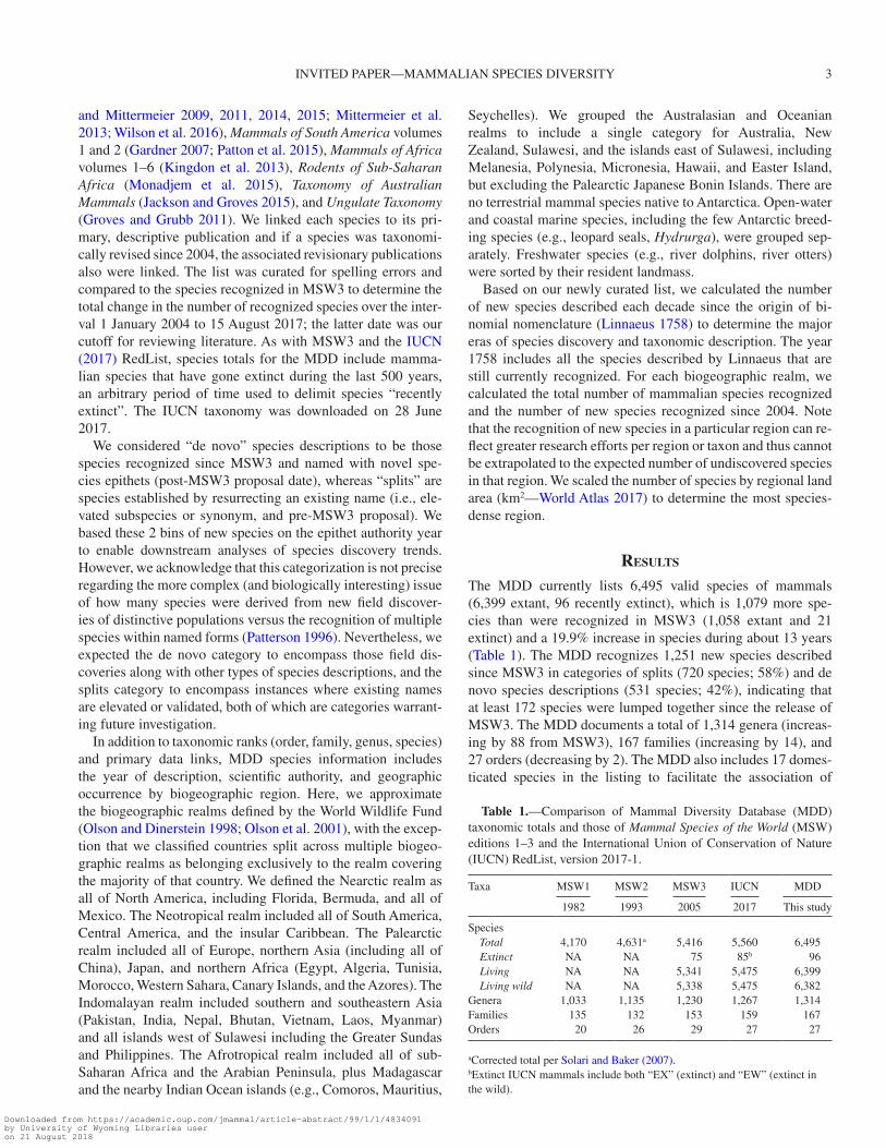
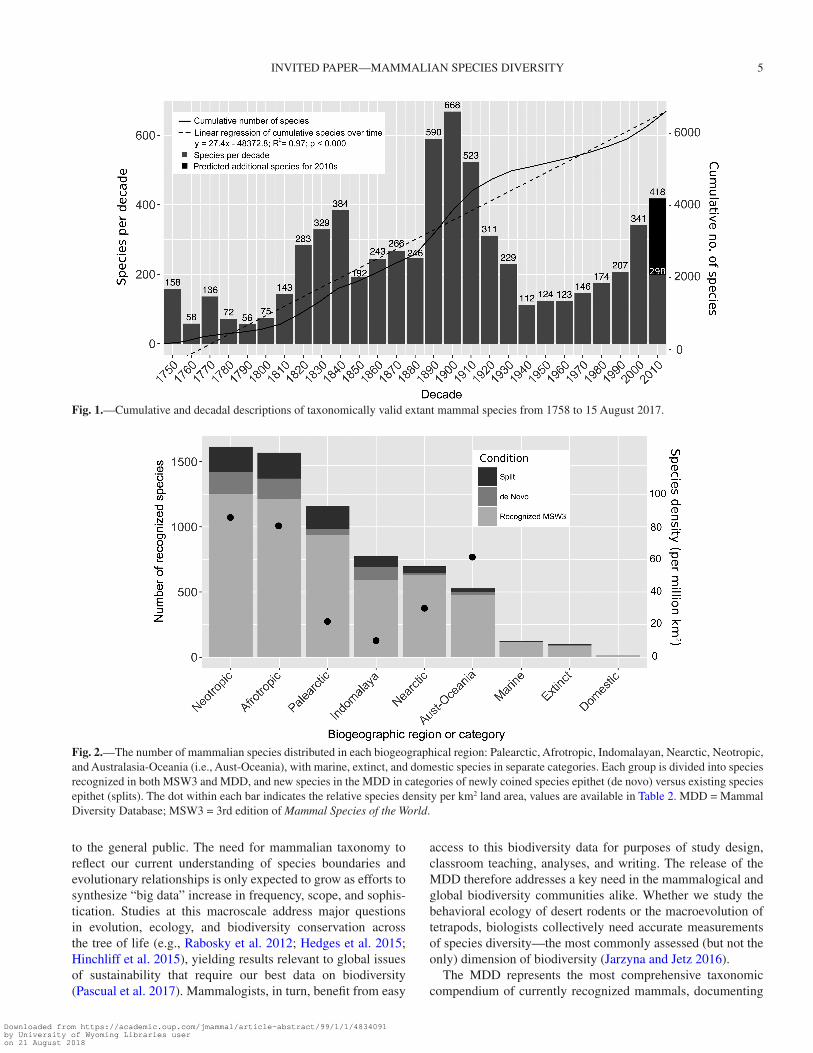

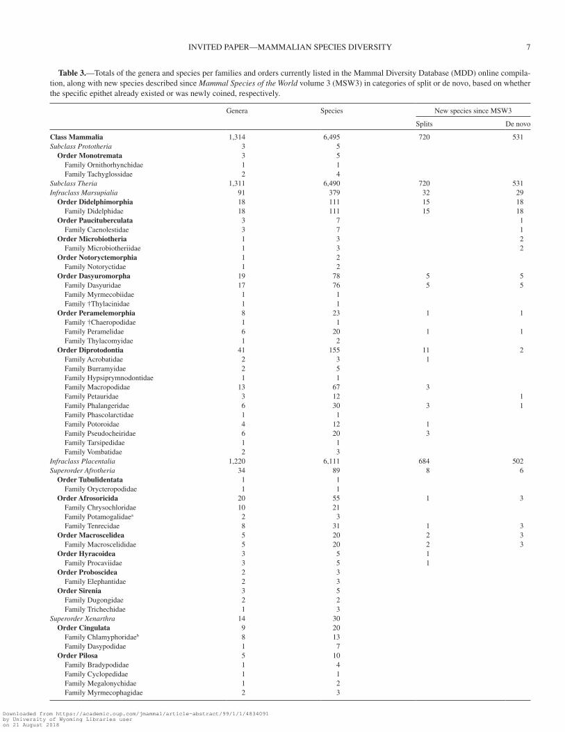
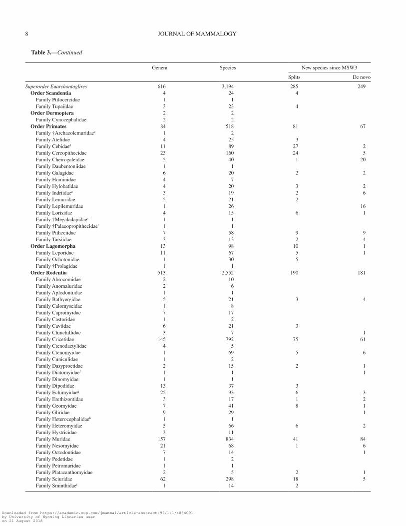
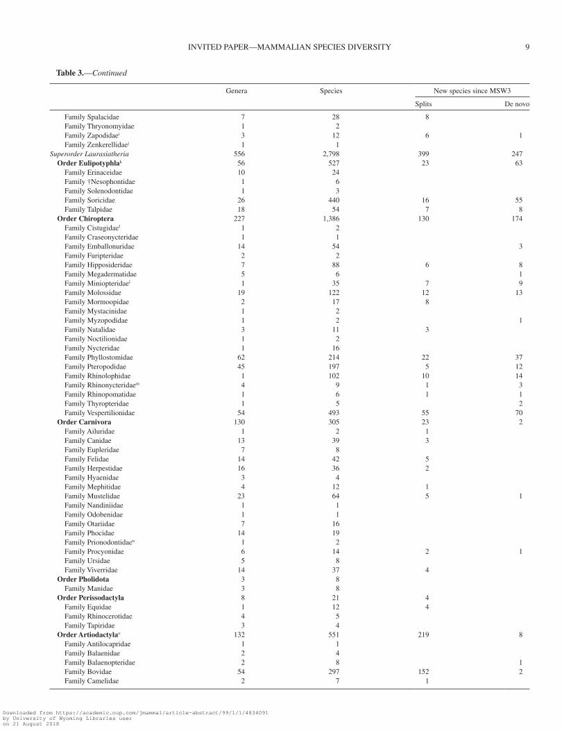
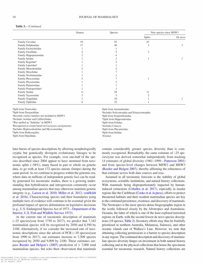


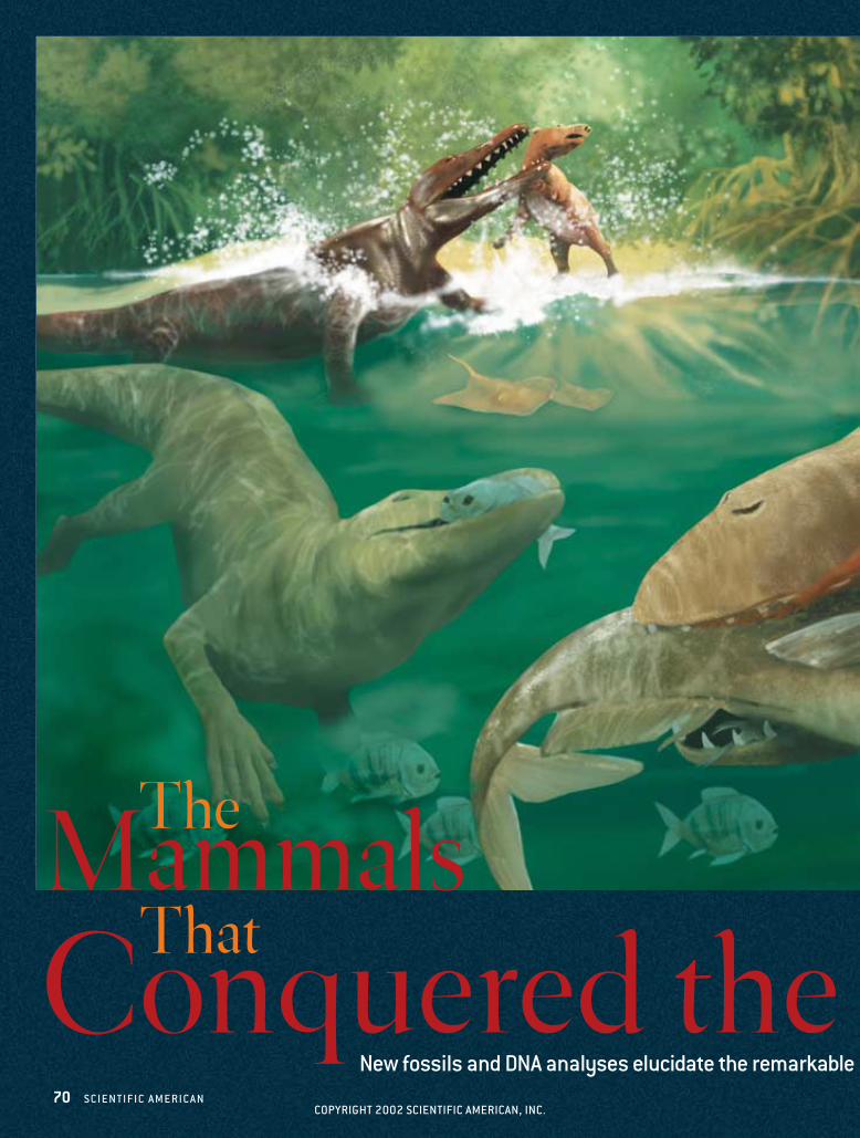
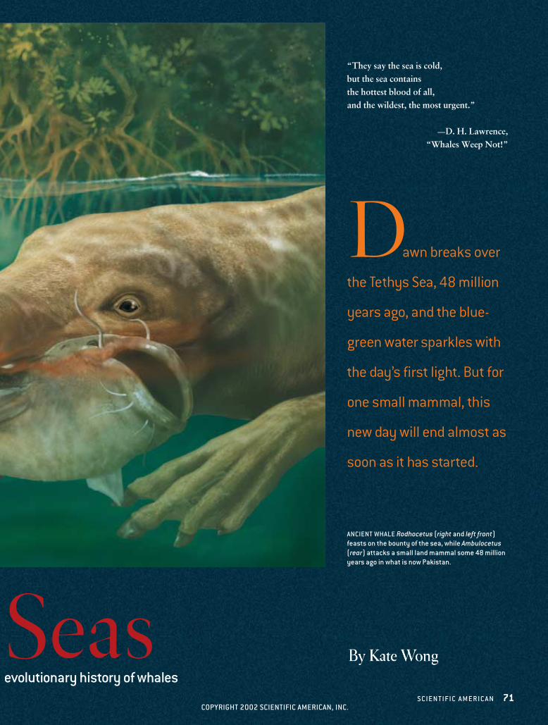

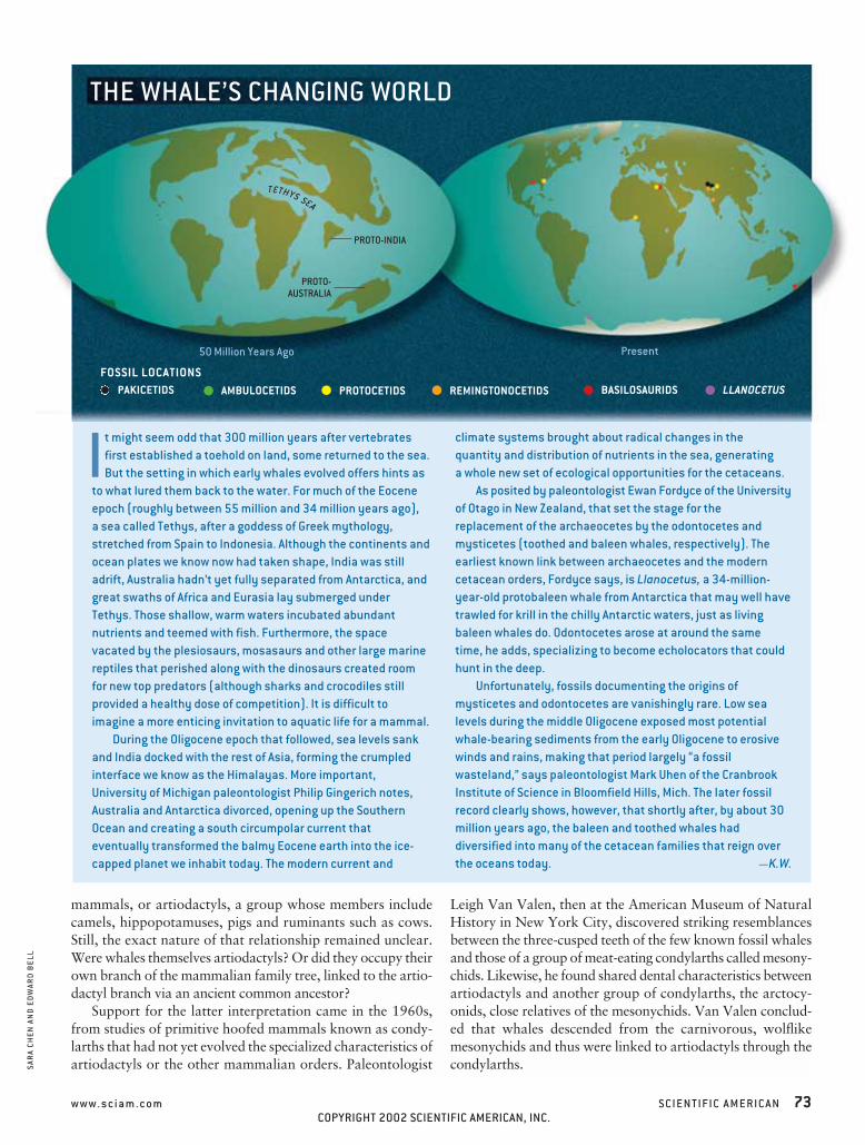


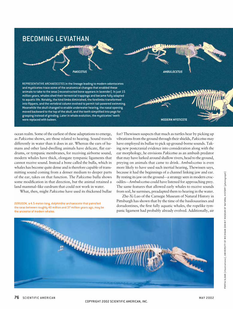

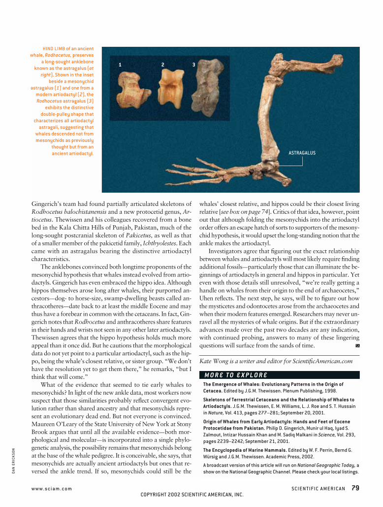

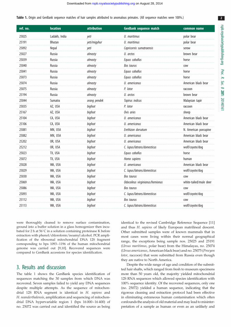


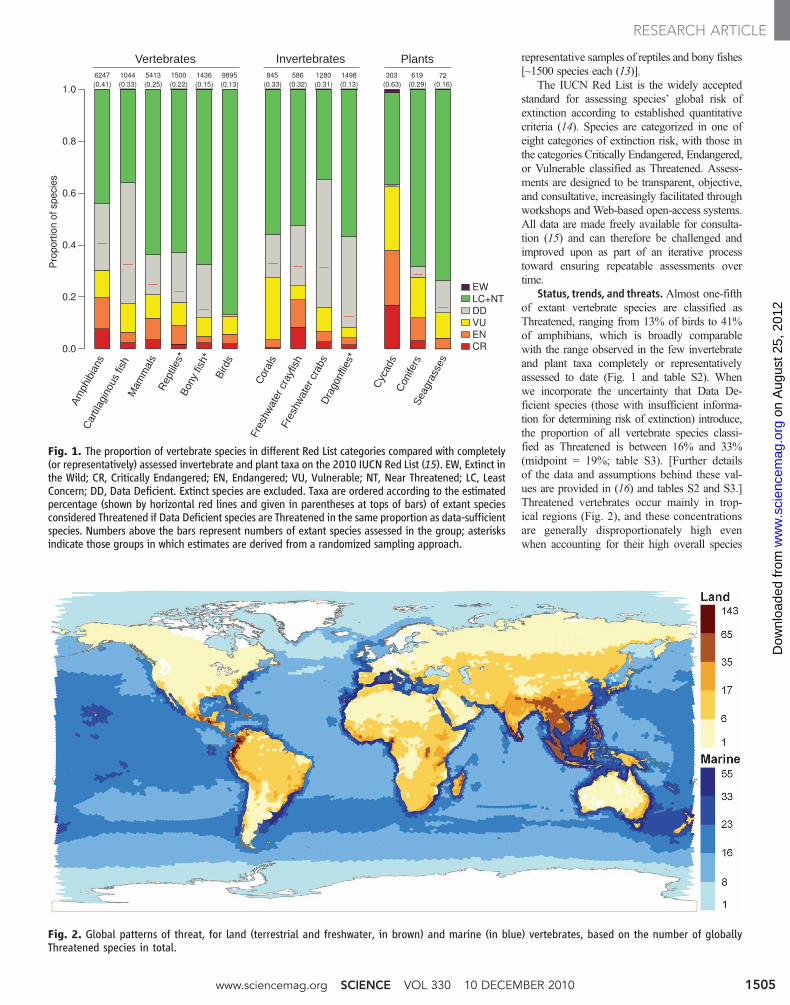
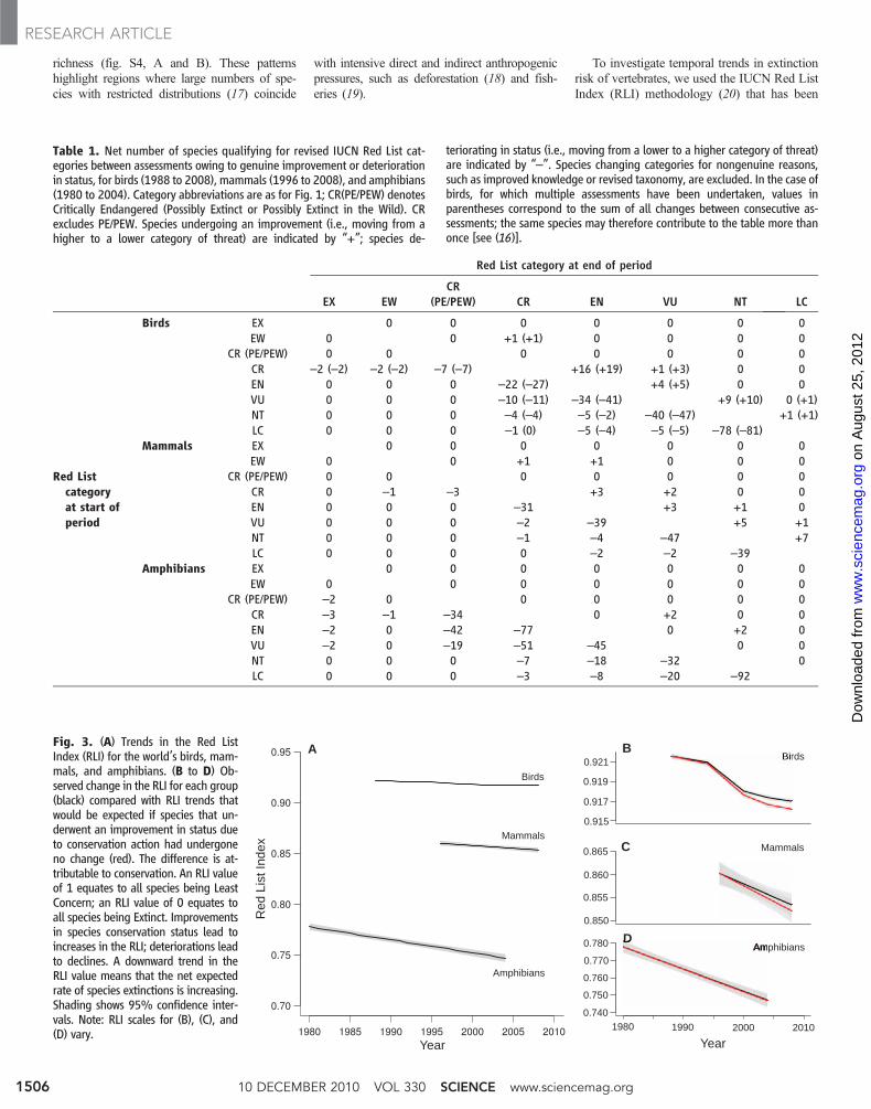

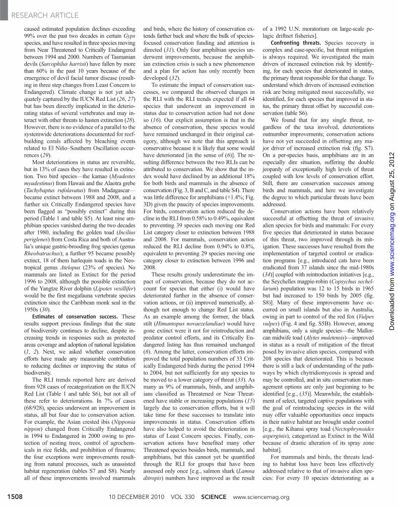
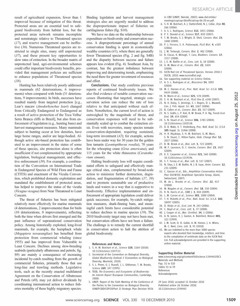
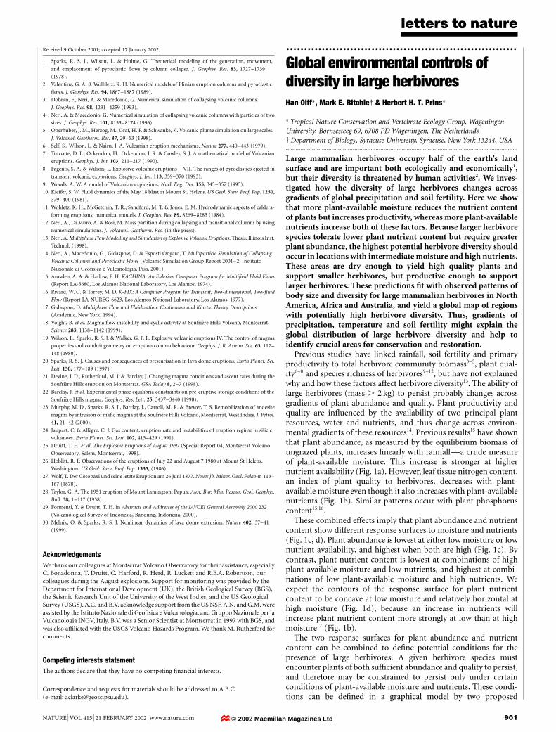

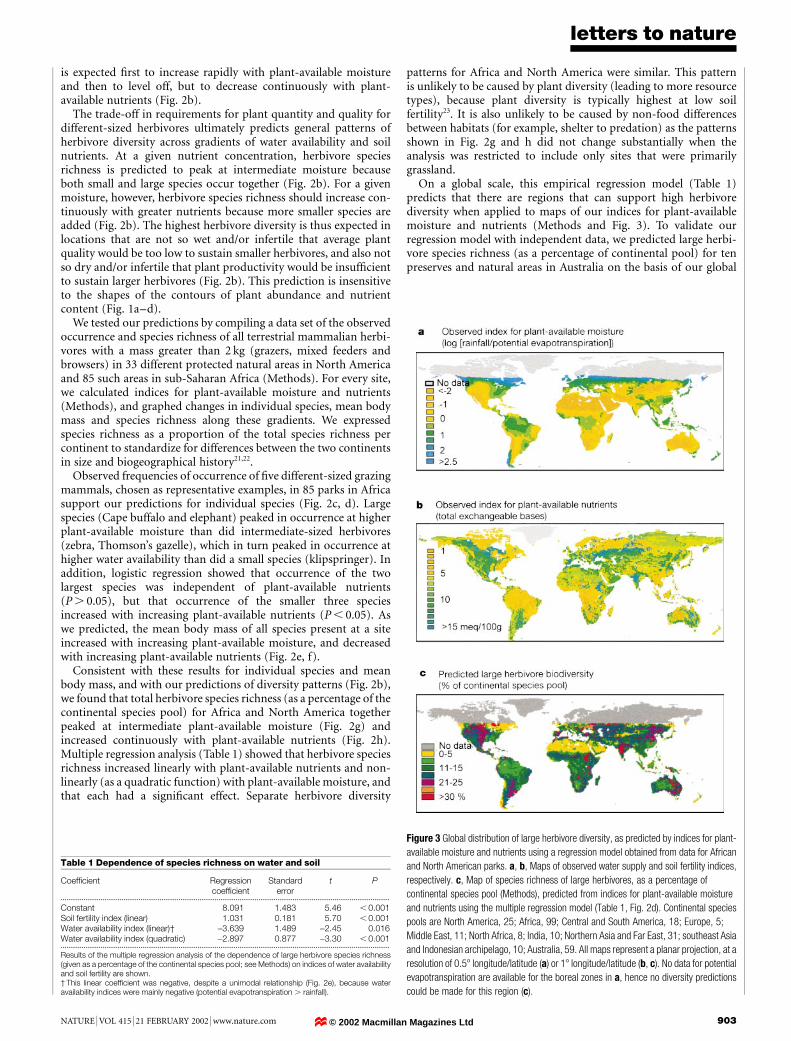


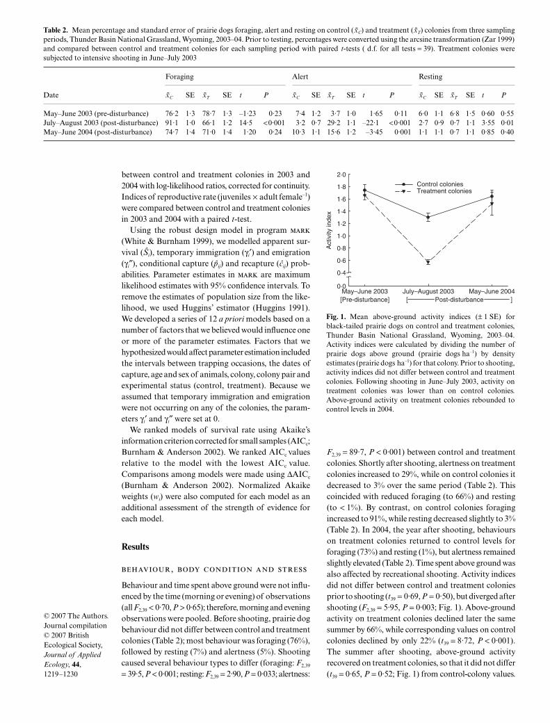

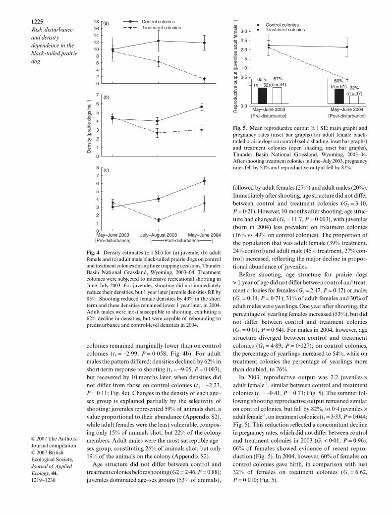


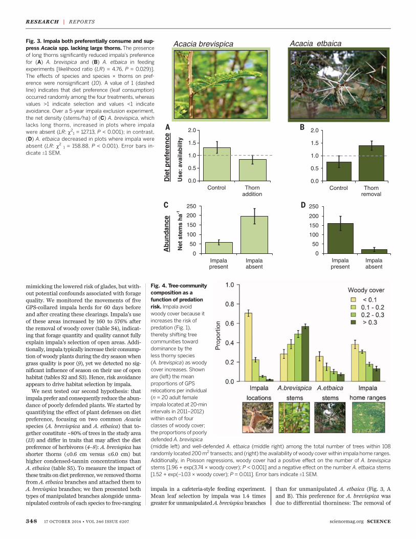
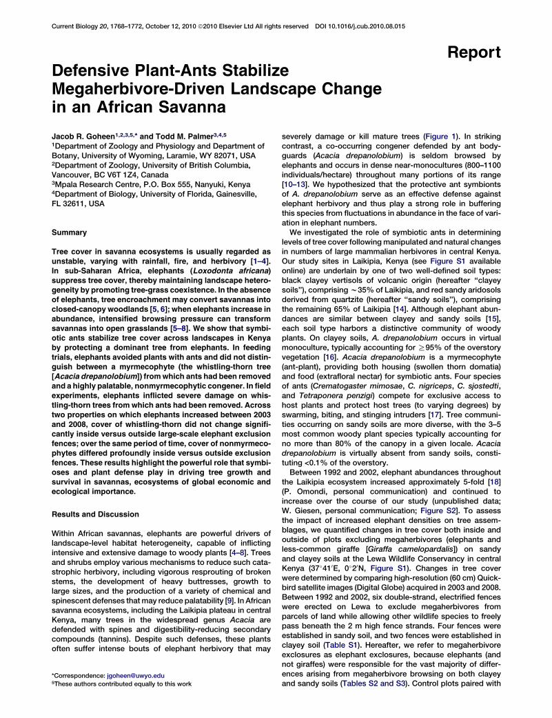
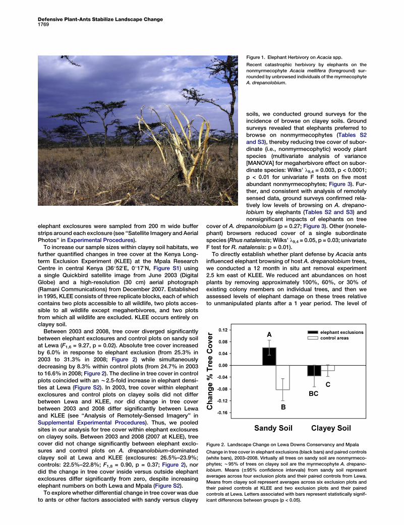
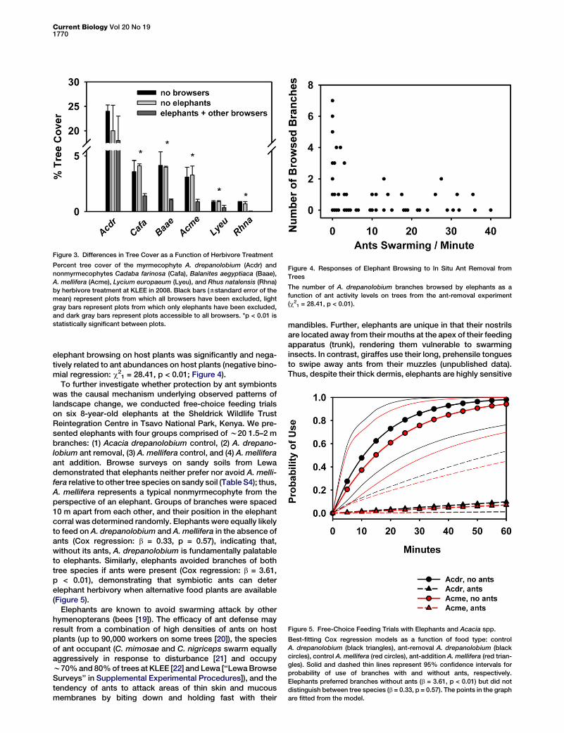
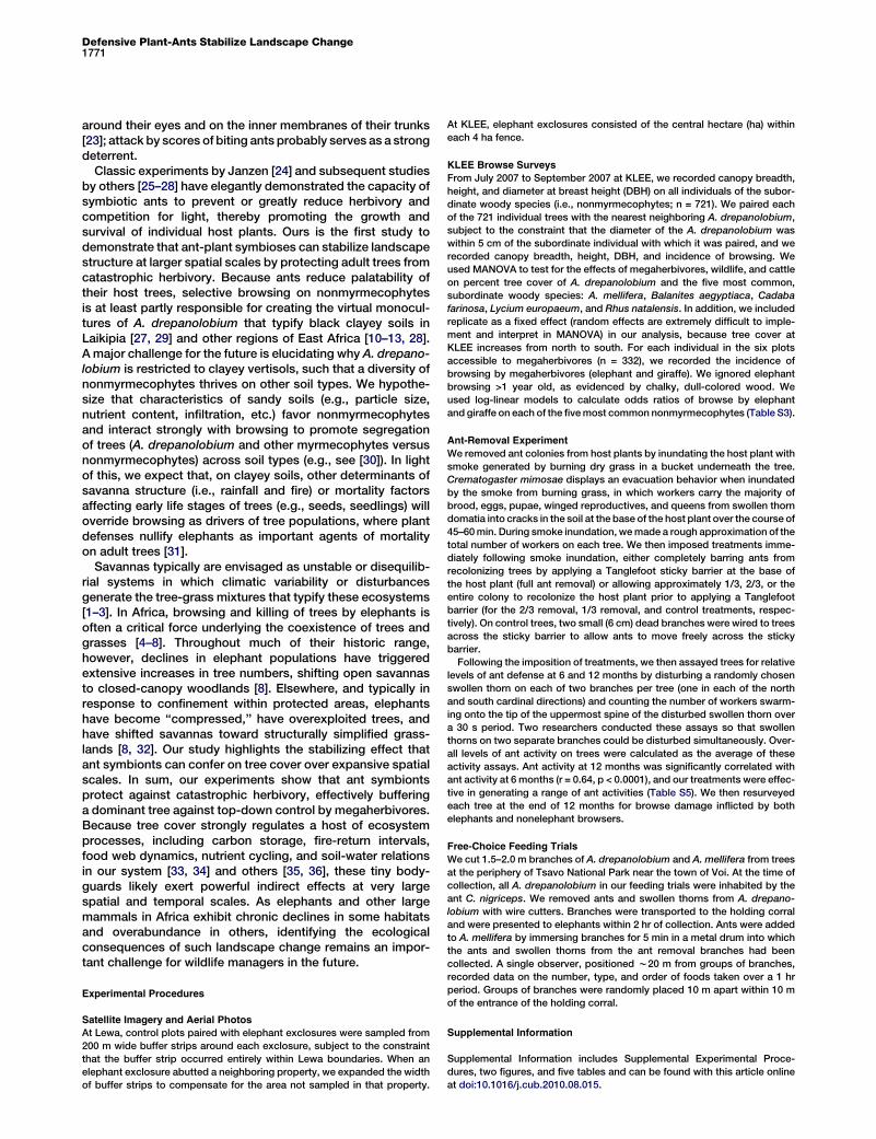
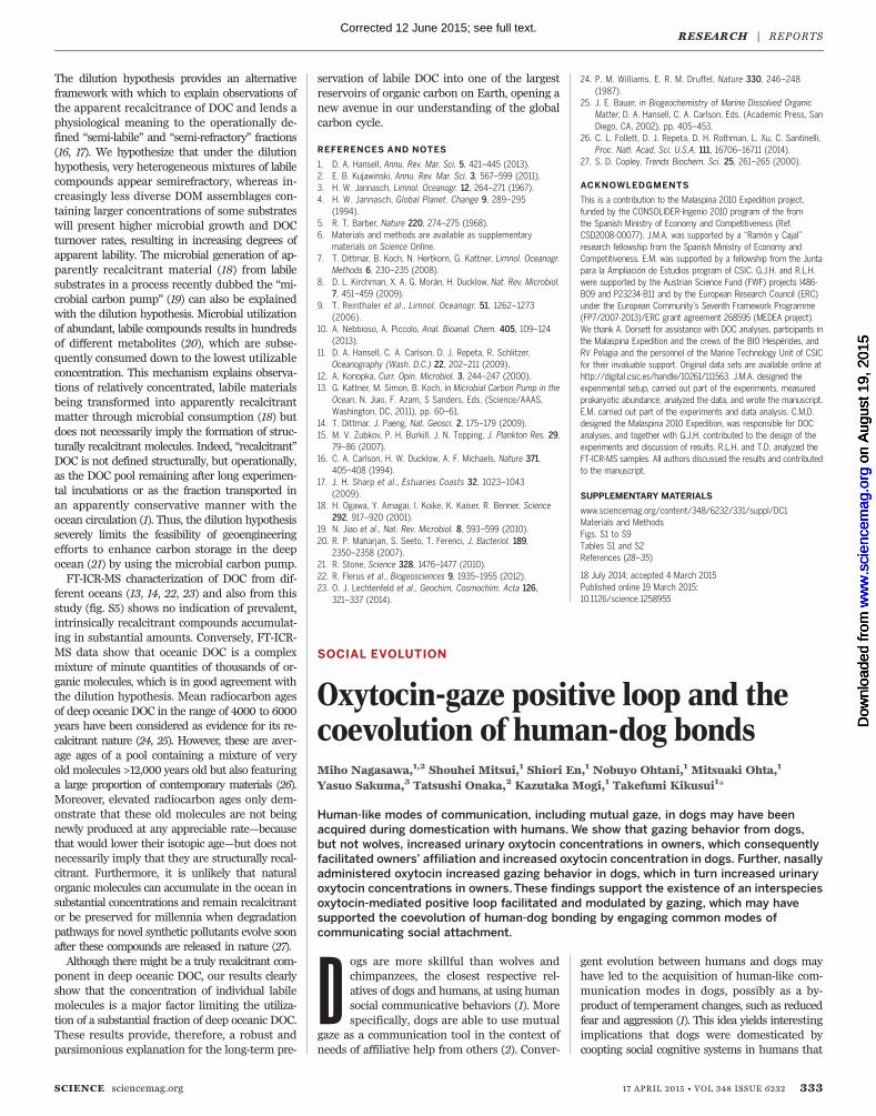


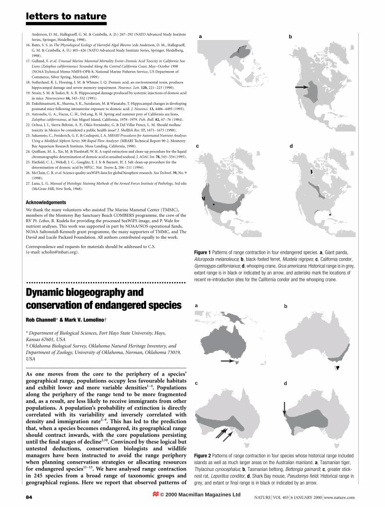


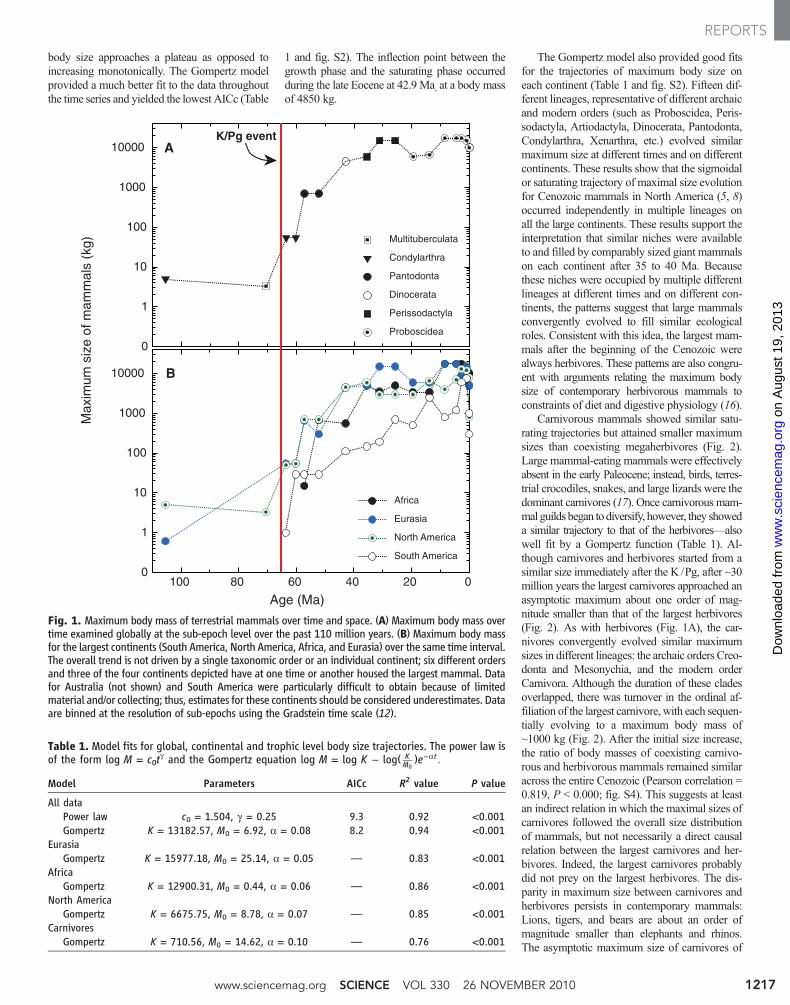
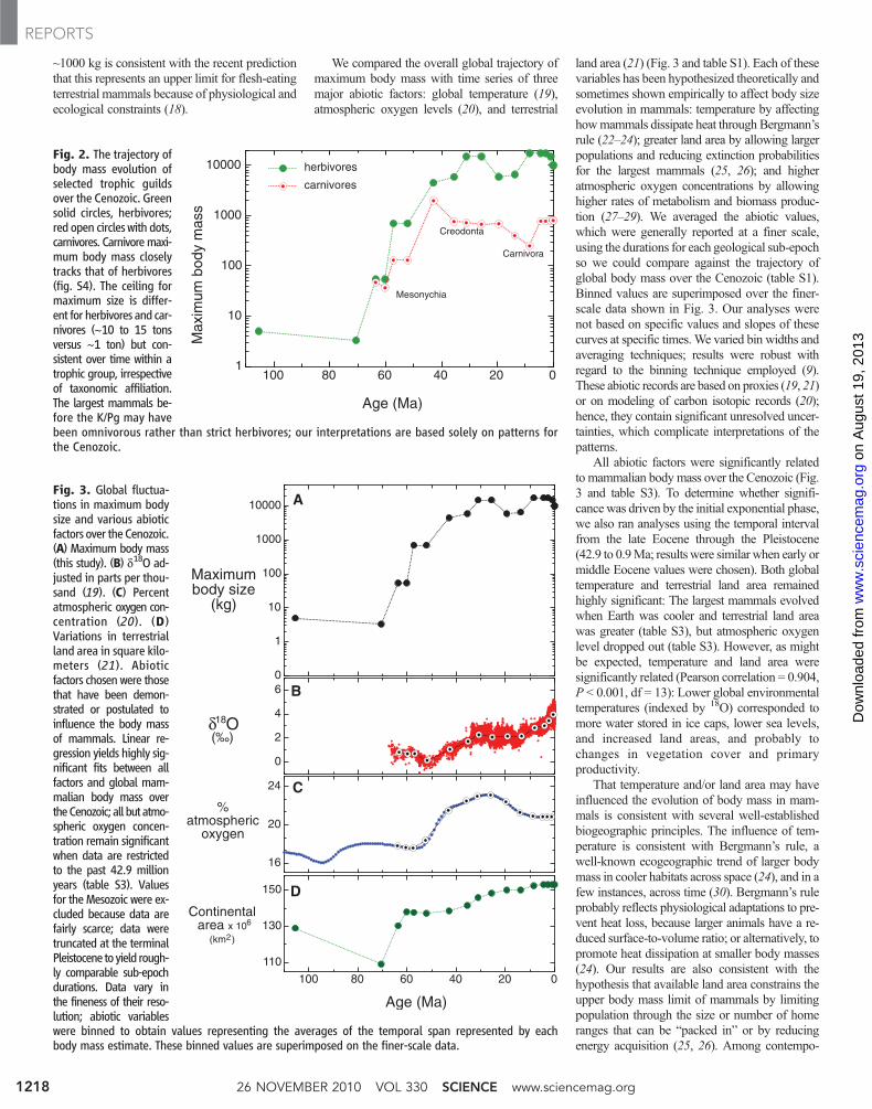

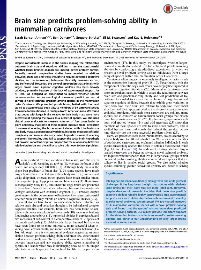
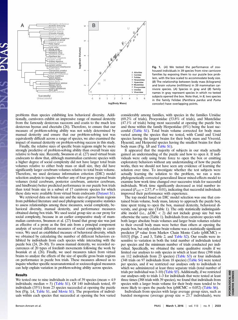
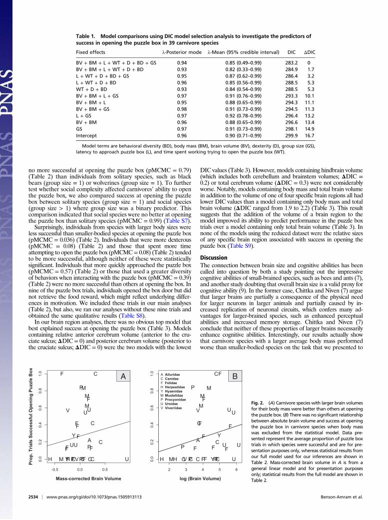
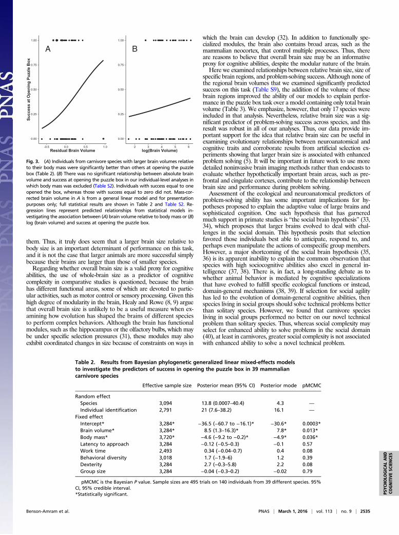
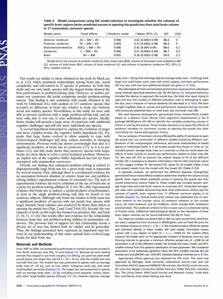
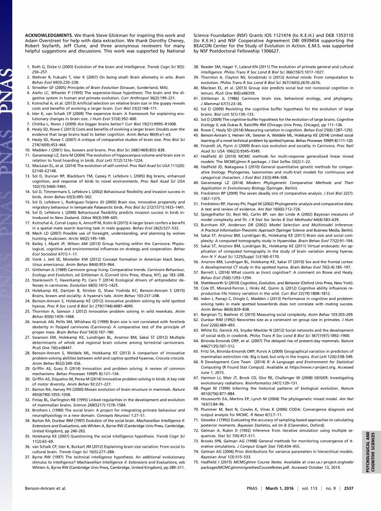


![GCSE EXAMPLE SPANISH RESPONSES...Escribe cuatro frases en español que describan la foto. [8 marks] Extract from mark scheme Question 01 For this question, students are required to](https://static.documents.pub/doc/80x56/6142043a2035ff3bc76266d7/gcse-example-spanish-responses-escribe-cuatro-frases-en-espaol-que-describan.jpg)


