Agitation 203 I I -.&.- I W 1. k IF NEEDED L-1.5WS L= 2w - 4 Figure 19. Suggested bafles for square and rectangular tanks. 5.0 FLUID SHEAR RATES Figure 20 illustrates flow pattern in the laminar flow region from a radial flat blade turbine. By using a velocity probe, the parabolic velocity distribution coming off the blades of the impeller is shown in Fig. 2 1. By taking the slope of the curve at any point, the shear rate may be calculated at that point. The maximum shear rate around the impeller periphery as well as the average shear rate around the impeller may also be calculated. An important concept is that one must multiply the fluid shear rate from the impeller by the viscosity of the fluid to get the fluid shear stress that actually carries out the process of mixing and dispersion. Fluid shear stress = p(fluid shear rate) Even in low viscosity fluids, by going from 1 cp to 10 cp there will be 10 times the shear stress of the process operating from the fluid shear rate of the impeller.
Transcript
Agitation 203
I I -.&.- I
W
1. k IF NEEDED
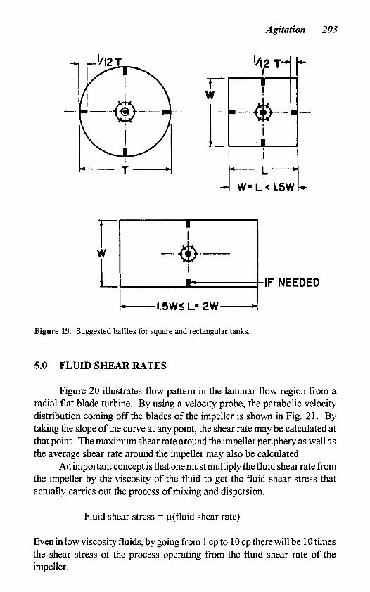
L-1.5WS L= 2w -4 Figure 19. Suggested bafles for square and rectangular tanks.
5.0 FLUID SHEAR RATES
Figure 20 illustrates flow pattern in the laminar flow region from a radial flat blade turbine. By using a velocity probe, the parabolic velocity distribution coming off the blades of the impeller is shown in Fig. 2 1. By taking the slope of the curve at any point, the shear rate may be calculated at that point. The maximum shear rate around the impeller periphery as well as the average shear rate around the impeller may also be calculated.
An important concept is that one must multiply the fluid shear rate from the impeller by the viscosity of the fluid to get the fluid shear stress that actually carries out the process of mixing and dispersion.
Fluid shear stress = p(fluid shear rate)
Even in low viscosity fluids, by going from 1 cp to 10 cp there will be 10 times the shear stress of the process operating from the fluid shear rate of the impeller.
204 Fermentation and Biochemical Engineering Handbook
Figure 20. Photograph of radial flow impeller in a baffled tank in the laminar region, madeby passing a thin plane of light through the center of the tank.
f:iY
M-~y
SHEAR RATE
~
Figure 21. Typical velocitypattem corning from the bladesofaradial flow turbine showingcalculation of the shear rate ~V/~Y.
Agitation 205
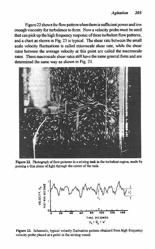
Figure 22 shows the flow pattern when there is sufficient power and lowenough viscosity for turbulence to fonn. Now a velocity probe must be usedthat can pick up the high frequency response of these turbulent flow patterns,and a chart as shown in Fig. 23 is typical. The shear rate between the smallscale velocity fluctuations is called microscale shear rate, while the shearrates between the average velocity at this point are called the macroscalerates. These macroscale shear rates still have the same general fonn and aredetermined the same way as shown in Fig. 21.
Figure 22. Photograph of flow patterns in a mixing tank in the turbulent region, made bypassing a thin plane of light through the center of the tank.
0..z
=» 0-u 2
>- ...~ "'u «0 ......A. I> :::
...
-t-
o """-~~.-~-..~-0 20 40 60 80 loo 120 140
TIME. SECONDS
U = 0 + u'X x
Figure 23. Schematic, typical velocity fluctuation pattern obtained from high frequencyvelocity probe placed at a point in the mixing vessel.
206 Fermentation and Biochemical Engineering Handbook
Table 2 describes four different macroscale shear rates of importance in a mixing tank. The parameter for the microscale shear rate at a point is the root mean square velocity fluctuation at that point, RMS.
Table 2. Average Point Velocity
Max. imp. zone shear rate
Ave. imp. zone shear rate
Ave. tank zone shear rate
Min. tank zone shear rate
5.1 Particles
The consideration of the macro- and microscale relationships in a mixing vessel leads to several helpful concepts. Particles that are greater 1,000 microns in size are affected primarily by the shear rate between the average velocities in the process and are an essential part of the overall flow throughout the tank and determine the rate at which flow and velocity distribute throughout the tank, and is a measure of the visual appearance of the tank in terms of surface action, blending or particle suspensions.
The other situation is on the microscale particles. They are particles less than 100 microns and they see largely the energy dissipation which occurs through the mechanism of viscous shear rates and shear stresses and ultimately the scale at which all energy is transformed into heat.
The macroscale environment is effected by every geometric variable and dimension and is a key parameter for successful scaleup of any process, whether microscale mixing is involved or not. This has some unfortunate consequences on scaleup since geometric similarity causes many other parameters to change in unusual ways, which may be either beneficial or
Agitation 20 7
detrimental, but are quite different than exist in a smaller pilot plant unit. On the other hand, the microscale mixing condition is primarily a function of power per unit volume and the result is dissipation of that energy down through the microscale and onto the level of the smallest eddies that can be identified as belonging to the mixing flow pattern. An analysis of the energy dissipation can be made in obtaining the kinetic energy of turbulence by putting the resultant velocity from the laser velocimeter through a spectrum analyzer. Figure 24a shows the breakdown of the energy as a function of frequency for the velocities themselves. Figure 24b shows a similar spectrum analysis of the energy dissipation based on velocity squared and Fig. 24c shows a spectrum analyzer result from the product of two orthogonal velocities, V, and Vz9 which is called the Reynolds stress (a function of momentum),
An estimation method of solving complex equations for turbulent flow uses a method called the K-E technique which allows the solution of the Navier-Stokes equation in the turbulent region.
5.2 Impeller Power Consumption
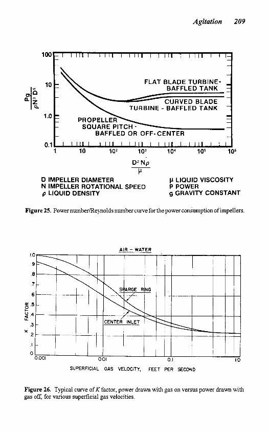
Figure 25 shows a typical Reynolds number-Power number curve for different impellers. The important thing about this curve is that it holds true whether the desired process job is being done or not. Power equations have three independent variables along with fluid properties: power, speed and diameter. There are only two independent choices for process considerations.
For gas-liquid operations there is another relationship called the K factor which relates the effect ofgas rate on power level. Figure 26 illustrates a typical K factor plot which can be used for estimation. Actual calculation of K factor in a particular case involves very specific combinations of mixer variables, tank variables, and fluid properties, as well as the gas rate being used.
Commonly, a physical picture of gas dispersion is used to describe the degree of mixing required in an aerobic fermenter. This can be helpful on occasion, but often gives a different perspective on the effect of power, speed and diameter on mass transfer steps. To illustrate the difference between physical dispersion and mass transfer, Fig. 27 illustrates a measurement made in one experiment where the height of a geyser coming off the top of the tank was measured as a function of power for various impellers. Reducing the geyser height to zero gives a uniform visual dispersion of gas across the surfBce ofthe tank. Figure 28 shows the actual data and indicates that the 8-inch impeller was more effective than the 6-inch impeller in this particular tank.
208 Fermentation and Biochemical Engineering Handbook
vz ( d B )
V Z & VR SPECTRUMS FOR 15.9 IN. A 2 0 0 (PBT)
- 70 L - 10 - 3 0
( d B ) -50
- 70
VR
0 4 10 15 20 HZ
N - 2.0 RPS C - 16 IN. ZC - 12.8 IN. RC = 5.6 IN.
RUN 23 JUL 87-4
POWER SPECTRUM VZ2& V R 2 FOR 15 IN. R 100 ( RUSHTON TURBINE 1
0
- 20
-40 - -60 I I I I 1
N = 2.0 RPS C = 16.0 IN ZC 16.75 IN: RC = 9.00 M.
REYNOLDS STRESS VZ xVR FOR 15.9 IN. A 2 0 0 (PBT)
I \ 8.00 HZ -10 1 ,073 F T 2 I S E C 2 i '
-70 0 5 10 15 20
HZ
N - 2.0 RPS (4 C 8 16 IN ZC 12.8 IN RC - 5.6 IN
RUN 23 JUL 87-4
Figure 24. Typical spectrum analysis of the velocity as a function of (a) velocity frequency fluctuation, (b) the frequency of the fluctuations using the square of the velocity to give the energy dissipation, and (c) the product of two orthogonal velocities versus the frequency of the fluctuations. The product of two orthogonal velocities is related to the momentum in the fluid stream.
Agitation 209
- I I I I I 1 I l l I I I I I I I I I I I I I l l I 1 l j - -
- - - FLAT BLADE TURBINE- - - BAFFLED TANK 1 -
-
CURVED BLADE -
TURBINE - BAFFLED TANK - ..
I I - - - - - - - BAFFLED OR OFF- CENTER
I I I I I I 1 1 1 1 I I I l l I I I l l I I I l l I I I
-
100
10
1 .o
0.1
DZ Np t.'
D IMPELLER DIAMETER LlOUlD VISCOSITY N IMPELLER ROTATIONAL SPEED p LlOUlD DENSITY
P POWER g GRAVITY CONSTANT
Figure 25. Power number/Reynolds number curve for the power consumption of impellers.
Figure 26. Typical curve of K factor, power drawn with gas on versus power drawn with gas off, for various superficial gas velocities.
21 0 Fermentation and Biochemical Engineering Handbook
Figure 27. Schematic of geyser height.
3.0
2.5
2.0 a W ln ln Q W
vj -I q a
1.5
0.5
I I 1 1 I I I 0 1 2 5 4 5 6
GEYSER HEIGHT, INCHES
Figure 28. Plot illustrating measurement of geyser height.
Agitation 21 I
Also, the 8-inch impeller with standard blades was more effective than the 8-inch impeller with narrow blades. These results all indicate that in this range of impeller-size-to-tank-size ratio, pumping capacity is more impor- tant than fluid shear rate for this particular criterion of physical dispersion.
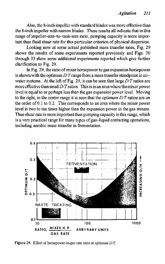
Looking now at some actual published mass transfer rates, Fig. 29 shows the results of some experiments reported previously and Figs. 30 through 33 show some additional experiments reported which give firther clarification to Fig. 29.
In Fig. 29, the ratio ofmixer horsepower to gas expansion horsepower is shown with the optimum D/Trange from a mass transfer standpoint in air- water systems. At the left of Fig. 29, it can be seen that large DIT ratios are more effective than small D/Tratios. This is in an area where the mixer power level is equal to or perhaps less than the gas expansion power level. Moving to the right, in the center range it is seen that the optimum D/T ratios are on the order of 0.1 to 0.2. This corresponds to an area where the mixer power level is two to ten times higher than the expansion power in the gas stream. Thus shear rate is more important than pumping capacity in this range, which is a very practical range for many types of gas-liquid contacting operations, including aerobic mass transfer in fermentation.
10 100 1000
RATIO, "' '' ARBITRARY UNITS G A S RATE
Figure 29. Effect of horsepower-to-gas rate ratio at optimum DIT.
212 Fermentation and Biochemical Engineering Handbook
Figure 30. Effect of sparge ring diameter on mass transfer performance of a flat blade turbine, based on gassed horsepower at gas velocity F = 0.02 ft/sec.
Figure 31. Effect ofhorsepower and impeller diameter onmass transfer coefficient at 0.04 Wsec gas velocity.
Agitation 213
J
v) J 0 I m J
- 0
l- 2 .08
a Y
h
I- v)L 0 2 .04 2 -
J,
h mg
CENTER INLET
.08 -
.04
.02 -
-
CENTER INLET A - F=.O8 F T / S E C .08 -
.O 4
.o 2 I/' "' l 'o i.0 410 8.b ;O 2 b
HP/ 1000 G A L S . GASSED
Figure 32. Effect ofhorsepower and impeller diameter on mass transfer coefficient at 0.08 Wsec gas velocity.,
." I
1.0 2.0 4.0 8.0 IO HP/1000 GALS. GASSED
Figure 33. Effect ofhorsepower and impeller diameter on mass transfer coefficient for gas velocity of 0.13 Wsec.
214 Fermentation and Biochemical Engineering Handbook
At the far right of Fig. 29 is shown high mixer power levels relative to the gas rate, and it can be seen that DlT makes no difference to the mass transfer. This occurs in some types of hydrogenation, carbonation, and chlorination. In those cases, the power level is so high relative to the amount of gas added to the tank that flow to shear ratio is of no importance.
In Figs. 30 through 33, the gas rate is successively increased in each of the four figures. At the low gas rate, the 4-inch impeller is more effective than the 6 or 8-inch impeller under all power levels. At the higher gas rates, the larger impellers become more effective at the lower gas rates, while the smaller impellers are more effective at the higher power levels, fitting generally into the scheme shown in Fig. 29.
A sparge ring about 80% ofthe impeller diameter is more effective than an open pipe beneath the impeller or sparge rings larger than the impeller. Figure 34 shows this effect and indicates that the desired entry point for the gas is where it can pass initially through the high shear zone around the impeller.
This has led to the common practice today of using the distribution of power in a three-impeller system, for example, 40% to the lower impeller and 30% to each of the two upper impellers, Fig. 35.
(P 0
Y
T = 4 6 0 m m Z=460mm
1 -
0.1 I I 1 1 I .2 .4 .8 1.0 2.0 K W I cu METER GASSED
Figure 34. Gas-liquid mass transfer data for 150 mm turbine in 460 mm tank at 0.07 m/ sec superficial gas velocity.
Agitation 21 5
f 30% 30%
40%
Figure 35. Typical power consumption relations for triple impeller installation, giving higher horsepower in proportion to the lower impeller.
In regard to tank shape, it has turned out over the years that about the biggest tank that can be shop-fabricated and shipped to the plant site over the highways is about 14 ft (4.3 m) in diameter. As fermentation volumes have gone from 10,000 gallons (38 m3) to 50 or 60 thousand gallons, tank shapes have tended to get very tall and narrow, resulting in Z/Tratios of 2: 1,3 : 1,4: 1, or even higher on occasion. This tall tank shape has some advantages and disadvantages, but tank shape is normally a design variable to be looked at in terms of optimizing the overall plant process design.
This leads to the concept of mass transfer calculation techniques in scaleup. Figure 36 shows the concept of mass transfer from the gas-liquid step as well as the mass transfer step to liquid-solid andor a chemical reaction. Inherent in all these mass transfer calculations is the concept of dissolved oxygen level and the driving force between the phases. In aerobic fermentation, it is normally the case that the gas-liquid mass transfer step from gas to liquid is the most important. Usually the gas-liquid mass transfer rate is measured, adriving force between the gas and the liquid calculated, and the mass transfer coefficient, &a or &a obtained. Correlation techniques use the data shown in Fig. 37 as typical in which &a is correlated versus power level and gas rate for the particular system studied.
216 Fermentation and Biochemical Engineering Handbook
LIQUID C
I I I I I I I I adc/de=k(c)a(c,)b
Figure 36. Schematic showing gas-liquid mass transfer step related to the other steps of liquid-solid mass transfer and chemical reaction.
20
1 1 10 100
POWER/ VOL., RELATIVE
Figure 37. Typical &a versus horsepower and gas velocity correlation; box on right indicates typical pilot plant experiments; box on left indicates typical full-scale range.
Agitation 21 7
If the data are obtained on small scale, then translation to larger scale equipment means an increase in superficial gas velocity, F, because of the change in liquid level in the large scale system. This normally pushes the data toward the left and would possibly result in a lower power level being required full-scale for the same mass transfer rate.
This has to be examined with great care, because any change in the power level will change the liquid-solid mass transfer rate; change the blend time, the shear rate and, therefore, the viscosity of non-Newtonian broth, and could necessitate many other process considerations.
5.3 Mass Transfer Characteristics of Fluidfoil Impellers
Experiments made with the sulfite oxidation technique evaluate the overall &a relationship for radial flow turbines and a very typical curve, shown in Fig. 38a gives the value of&a versus power and various gas rates. One will notice that there is a break in the curve which occurs about at the point where the power of the mixer is approximately two or three times higher than the power in the gas stream. A curve taken on similar conditions for the A3 15 impeller does not show the break point (Fig. 38b), and matching of the two curves shows that at the low end of the power levels the A3 15 results in a higher mass transfer relationship, while at higher power levels, the R100 is somewhat better. However, with &20%, which is with reasonable accuracy for these kind of measurement comparisons, the mass transfer performance is quite similar. The difference of performance on a given fermentation application should thus be higher or lower in terms of the mass transfer coefficient and needs to be studied in detail when a retrofit is desired.
One large difference between A3 15 and R100 impellers in fermentation is the blend time. Every RlOO impeller sets up two flow pattern zones. Thus, in a large fermentation tank with three or four RlOO impellers there are six to eight separate mixing zones/cells in the vessel. If the A3 15 impeller is used for the one or more different impeller positions, it sets up one overall flow pattern which gives one complete mixing zone and results in a blend time on a batch basis of approximately one-half to one-third the time it takes on the RlOO configuration. It is quite typical in current practice to use a radial flow turbine at the bottom while using a series of A3 15 impellers (either one, two or three, on the top positions). This has the overall tendency to reduce the macro- and microscale shear rates and also can either increase productivity at the same power level or retain the original productivity at a reduced power level. This, in a fermentation process, is of very great importance economically.
218 Fermentation and Biochemical Engineering Handbook
- F 1.0 1
.045 m / s
.034 m / s
.018 m / s
.012 m / s
DUAL R100s D / T - 0.33 Z / T - 1.56 -
I I I I I I 1 1 1 1 c
kGa
pmol 0 2 bar m3s
0.1
1 P / V ( k W / m 3 )
1 .o
ki;a
gmol 0~ bar m3s
0.1
- F .045 m / s .034 m / s
.018 m / s
.012 m / s
DUAL A315s D l / T - 0.44 D 2 / T - 0.37 Z / T - 1.56
1 I I 1 I I I - 1 10
P / V ( k W / m 3 )
Figure 38. Typical curves of &a versus power and various gas rates for radial flow turbines, (a) R100; (b) A-3 15.
Agitation 219
However, before retrofitting a large fermentation tank it should be realized unless there is some process data arising from understanding the relationship between the mass transfer and the biological oxidation require- ment, retrofitting existing radial flow turbine installations withA3 15 impeller types does not always give an improvement in process result. The average is normally about two or three times as frequent for a plus result as for neutral or negative results.
It is very difficult to study the effect of fluidfoil impellers in the pilot plant since the pilot plant in general has much shorter blend time and a much more uniform blending composition than appears in the full scale tank. Thus, putting fluidfoil impellers in the pilot plant improves the blending under a situation where the blending is already much improved over full scale performance.
6.0 FULL-SCALE PLANT DESIGN
There are four ways in which mixers are often specified when considering installation of more productive units in a fermentation plant. This can involve either a larger tank with a suitable mixer or improvement of the productivity of a given tank by a different combination of mixer horsepower and gas rate. These are listed below:
a. Change in productivity requirements based on production data with a particular size fermenter in the plant.
b. New production capacity based on pilot plant studies. c. Specification of agitator based on the sulfite absorption
d. Specification of the oxidation uptake rate in the actual rate in aqueous sodium sulfite solution.
broth for the new system.
6.1 Some General Relationships in Large Scale Mixers Compared to Small Scale Mixers
In general, a large scale mixing tank will have a lower pumping capacity per unit volume than a small tank. This means that its blend time and circulation time will be much larger than in a pilot tank.
There is also a tendency for the maximum impeller shear rate to go up while the average impeller zone shear rate will go down on scaleup. In
220 Fermentation and Biochemical Engineering Handbook
addition, the average tank zone shear rate will go down as will the minimum tank zone shear rate.
This means that there is a much greater variety of shear rates in the larger tank, and in dealing with pseudoplastic sluny it will have a quite different viscosity relationship around the tank in the big system compared to the smaller system.
Microscale shear rates operate in the range of 300 microns or less, and are governed largely by the power input.
The power input from the gas per unit volume will increase on scaleup. This is because there is a greater head pressure on the system, and there is also an increasing gas velocity.
It may be that the power level for the mixer may be reduced since the energy from the gas going through the tank is higher in order to maintain a particular mass transfer coefficient, &a; however, this changes the relative power level compared to the gas and other mass transfer rates, such as the liquid-solid mass transfer rate. The capacity for the blending type flow pattern is not affected in the same way with changes in the mixer power level as is the gas-liquid mass transfer coefficient.
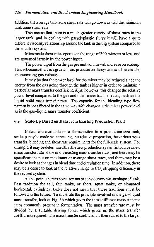
6.2 Scale-up Based on Data from Existing Production Plant
If data are available on a fermentation in a production-size tank, scaleup may be made by increasing, in a relative proportion, the various mass transfer, blending and shear rate requirements for the fill-scale system. For example, it may be determined that the new production system is to have a new mass transfer rate of x% of the existing mass transfer rates, and there may be specifications put on maximum or average shear rates, and there may be a desire to look at changes in blend time and circulation time. In addition, there may be a desire to look at the relative change in C 0 2 stripping efficiency in the revised system.
At this point, there is no reason not to consider any size or shape of tank. Past tradition for tall, thin tanks, or short, squat tanks, or elongated horizontal, cylindrical tanks does not mean that those traditions must be followed in the future. To illustrate the principle involved in the gas-liquid mass transfer, look at Fig. 36 which gives the three different mass transfer steps commonly present in fermentation. The mass transfer rate must be divided by a suitable driving force, which gives us the mass transfer coefficient required. The mass transfer coefficient is then scaled to the larger
Agitution 221
tank size and is normally related to superficial gas velocity to an exponent, power per unit volume to an exponent, and to other geometric variables such as the D/T ratio of the impeller.
A thorough analysis takes a look at every proposed tank shape, looks at the gas rate range required, calculates the gas phase mass transfer driving force, and then calculates the required &a to meet that. Reference is made to data on the mixer under the condition specified and to various DIT ratios to obtain the right mixer horsepower level for each gas rate.
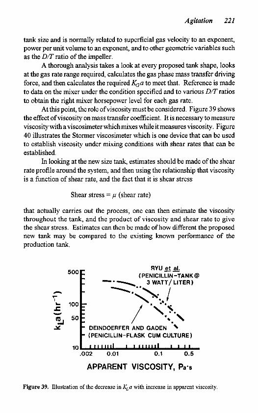
Atthis point, the role ofviscosity must be considered. Figure 39 shows the effect ofviscosity on mass transfer coefficient. It is necessary to measure viscosity with a viscosimeter which mixes while it measures viscosity. Figure 40 illustrates the Stormer viscosimeter which is one device that can be used to establish viscosity under mixing conditions with shear rates that can be established.
In looking at the new size tank, estimates should be made of the shear rate profile around the system, and then using the relationship that viscosity is a function of shear rate, and the fact that it is shear stress
Shear stress = p (shear rate)
that actually cames out the process, one can then estimate the viscosity throughout the tank, and the product of viscosity and shear rate to give the shear stress. Estimates can then be made of how different the proposed new tank may be compared to the existing known performance of the production tank.
n r
I L
Y r
5 3
RYU gta (PENICILLIN-TANK @
DEINDOERFER AND GADEN -\ (PENICILLIN-FLASK CUM CULTURE)
.002 0.01 0.1 0.5
APPARENT VISCOSITY, Pa*s
Figure 39. Illustration of the decrease in K,a with increase in apparent viscosity.
222 Fermentation and Biochemical Engineering Handbook
One relationship that cannot be changed simply going from a small to large scale is the fact that the Reynolds number normally increases in the large tank over what it was in the small tank. The Reynolds number is typically anywhere from 10 to 50 times higher in the large vessel than in the small. This means that the fluid in the pilot scale will appear much more viscous in terms of flow pattern and many other parameters than it will in the full scale tank. It is usually not practical where conducting a process to change viscosity between pilot plant and full scale, but if one is interested in getting an idea of the flow pattern and some of the macroscale effects, then a synthetic fluid of a lower viscosity than the actual could be substituted in the full scale work to give a better picture of the expected flow pattern.
Agitation 223
At this point discussion of the quantitative and qualitative nature of available data is desirable. The user, production, research and engineering, and purchasing department should have discussions with the suppliers and technical personnel to arrive at satisfactory combinations of proposals.
6.3 Data Based on Pilot Plant Work
To keep ratios of impellers, gas bubbles and solid clumps in the fermentation related to full scale, the impeller size and blade width in the small scale must always have a physical dimension two or three times bigger than the particle size of concern.
It is possible to model the fermentation biological process from a fluid mechanics standpoint, even though the impeller is not related properly geometrically to the gas-liquid mass transfer step. Thus, one scale of pilot plant might be usable for one or two of the fermentation mass transfer steps, and/or chemical reaction steps, but might not be suitable for analysis of other mass transfer steps. The decision, then, is basedon how suitable existing data are for any steps which are not modeled properly in the pilot plant.
Ideally, data should be taken during the course of the fermentation about gas rate, gas absorption, dissolved oxygen level, dissolved carbon dioxide level, yield of desired product, and other parameters which might influence the decision on the overall process. Figure 4 1 shows a typical set of data for this situation.
A TYPICAL FERMENTATION G57
v)
I I I
TIME
Figure 41. Schematic of typical data from fermentation showing the change in oxygen content of gas, CO, content in liquid and fermentation yield.
224 Fermentation and Biochemical Engineering Handbook
If the pilot plant is to duplicate certain properties of fluid mixing, then it may be necessary to use non-geometric impellers and tank geometries to duplicate mixing performance and not geometric similarity. As a general rule, geometric similarity does not control any mixing scaleup property whatsoever.
It may also not be possible to duplicate all of the desired variables in each run, so a series of runs may be required changing various relationships systematically and then a synthesis made of the overall results.
One variable in particular is important. The linear superficial gas velocity should be run in a few cases at the levels expected in the full-scale plant. This means that foaming conditions are more typical of what is going to happen in the plant and the fermenter should always be provided with enough head space to make sure the foam levels can be adequately controlled in the pilot plant. As a general rule, foam level is related to the square root of the tank diameter on scaleup or scale-down.
In duplicating maximum impeller zone shear rates on a small scale, there may be a very severe design problem in the mechanics of the mixer, or the shaft speed, mechanical seals and other things. This means that careful consideration must be given to the type of runs to be made and whether the pilot plant or the semi-work-scale equipment must be available at all times to duplicate the maximum impeller zone shear rates in the plant or whether this sort of data will be obtained on a different type of unit dedicated to that particular variable.
Figure 37 shows what often happens in the pilot plant in terms of correlatingmass transfer coefficient, &a, with power andgas rate in the pilot plant. This curve is then translated to a suitable relationship for full scale. It is possible to consider that with the higher superficial gas velocity, the power level may be reduced in the full scale to keep the same mass transfer coefficient. The box on the right in Fig. 37 shifts to the box on the left. This should be considered, but it should be borne in mind that this changes the ratio of the mixer power to gas power level in the system; changes the blend time; changes the flow pattern in the system; the foaming characteristics and also can markedly affect the liquid-solid mass transfer rate if that is important in the process.
In all cases, a suitable mass transfer driving force must be used. Figure 42 illustrates a typical case for fermentation processes and illustrates that there is a marked difference between the average driving force, the log-mean driving force, and the exit gas driving force. In a large fermenter, it is this author’s experience that gas concentrations are essentially step-wise stage functions and a log-mean average driving force has been the most fruitful.
Agitation 225
Figure 43 illustrates a small laboratory fermenter with a Z/T ratio of 1, and in this case, depending on the power level, an estimate must be made of the gas mixing characteristics and an evaluation made ofthe suitability of the exit gas concentration for the driving force compared to the log-mean driving force. This is one area which needs to be explored in the pilot program and the calculation procedures.
Xz.15 Ap= .025 pp = .225
P= 2 Xz.21 A p =.22 I pp=.42
Figure 42. Typical driving force for larger fermenter.
Ap=0.025 I---- I
A p =0.22 AIR
Figure 43. Driving force for small laboratory fermenter.
226 Fermentation and Biochemical Engineering Handbook
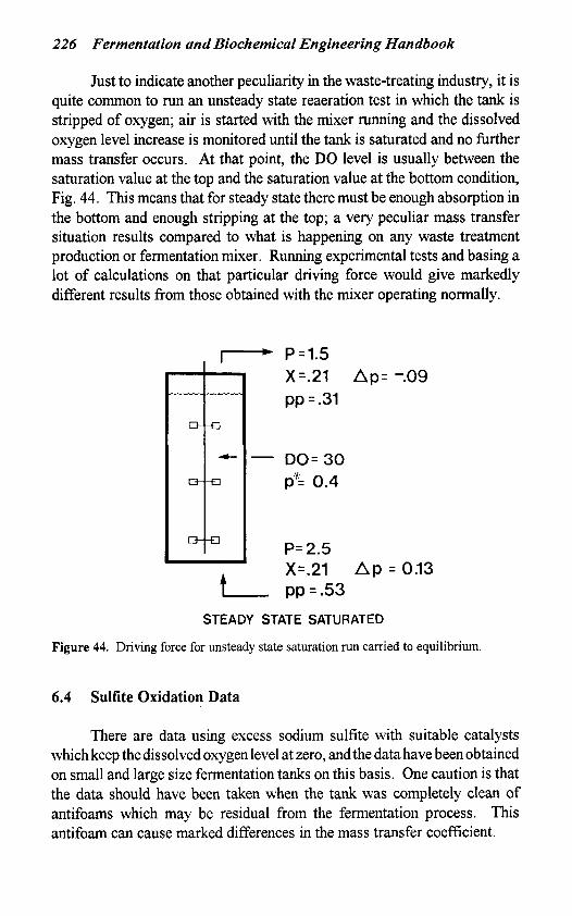
Just to indicate another peculiarity in the waste-treating industry, it is quite common to run an unsteady state reaeration test in which the tank is stripped of oxygen; air is started with the mixer running and the dissolved oxygen level increase is monitored until the tank is saturated and no further mass transfer occurs. At that point, the DO level is usually between the saturation value at the top and the saturation value at the bottom condition, Fig. 44. This means that for steady state there must be enough absorption in the bottom and enough stripping at the top; a very peculiar mass transfer situation results compared to what is happening on any waste treatment production or fermentation mixer. Running experimental tests and basing a lot of calculations on that particular driving force would give markedly different results from those obtained with the mixer operating normally.
- P=1.5 Xz.21 Ap= -.09 pp = .31
- DO=30 p"= 0.4
P= 2.5 X=.21 Ap = 0.13
I- pp=.53
STEADY STATE SATURATED
Figure 44. Driving force for unsteady state saturation run carried to equilibrium.
6.4 Sulfite Oxidation Data
There are data using excess sodium sulfite with suitable catalysts which keep the dissolved oxygen level at zero, and the data have been obtained on small and large size fermentation tanks on this basis. One caution is that the data should have been taken when the tank was completely clean of antifoams which may be residual from the fermentation process. This antifoam can cause marked differences in the mass transfer coefficient.
Agitation 22 7
If someone has a relationship between the sulfite oxidation number and the performance required in the fermenter, this is a perfectly valid way to specify equipment and tests can be run to give an indication of the overall mass transfer rate ensuing.
6.5 Oxygen Uptake Rate in the Broth
If it is desired to relate fermenter performance to oxygen uptake rate in the broth, this number can be specified along with suitable desired gas rates, and the mixer estimated, based on this performance. Again, someone must have the link between this particular mass transfer specification and the actual performance of the fermenter.
Ifthis number is based on pilot plant data, then the effect ofthe different shear rates and different blend times on the mass transfer relationship, viscosity and the resulting fermentation must be considered.
6.6 Some General Concepts
Table 3 gives some typical power levels used in various gas-liquid mixing operations, including waste-treating and fermentation, to give some idea of the range of variables. Obviously, the tremendous variety of units used precludes an attempt to guess at a mixer based on general overall approximations.
The lower impeller does the major part of the work on dispersing gas in the system and it is typical practice today to put a high proportion of the power into the lower impeller, somewhat similar to what is shown in Fig. 35. Multiple impellers do have zoning action in terms of blending, which is not a great factor in a fermentation which takes seven days, but there are instantaneous differences in the mass transfer, blending and concentration profiles in a tank with multiple impellers.
228 Fermentation and Biochemical Engineering Handbook
In addition, the role of the lower impeller in both mass transfer and mixing must be considered and the desirability of having multiple impellers in the tank can be considered.
If it is desired to consider axial flow impellers in a gas-liquid system for any reason, it should be remembered that the upward flow of gas tends to negate the downward action ofthe pumping capacity ofthe axial flow turbine. A radial flow turbine must have three times more power than the power in the gas stream for the mixer power level to be h l ly effective. On the other hand, the axial flow impeller must have eight to ten times more power than in the gas stream for it to establish the axial flow pattern.
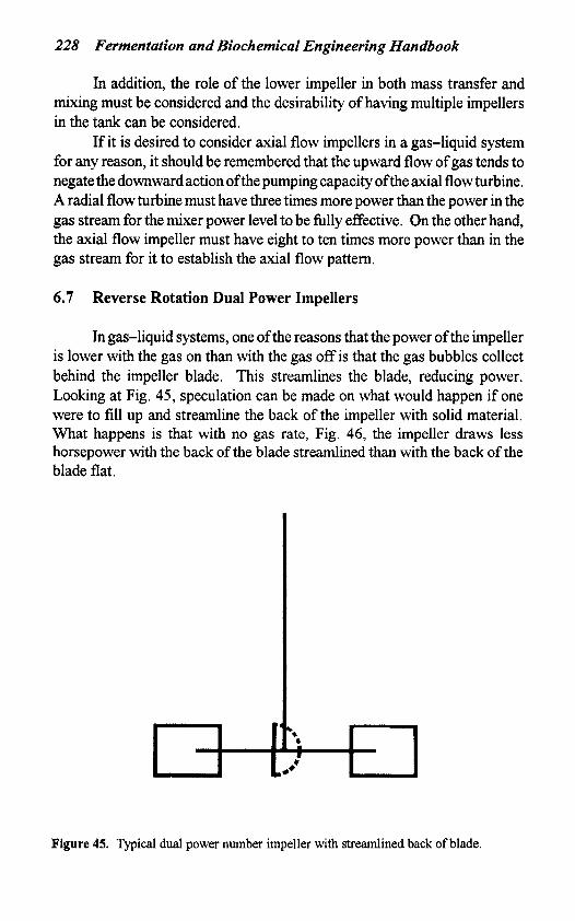
6.7 Reverse Rotation Dual Power Impellers
In gas-liquid systems, one of the reasons that the power of the impeller is lower with the gas on than with the gas off is that the gas bubbles collect behind the impeller blade. This streamlines the blade, reducing power. Looking at Fig. 45, speculation can be made on what would happen if one were to fill up and streamline the back of the impeller with solid material. What happens is that with no gas rate, Fig. 46, the impeller draws less horsepower with the back of the blade streamlined than with the back of the blade flat.
Figure 45. Typical dual power number impeller with streamlined back of blade.
Agitation 229
AIR - WATER
1 .o .9
.a
.4
.3
.2 .1 0
Y
0.001 0.01 0.1 SUPERFICIAL GAS VELOCITY, METERS/SEC.
Figure 46. Power characteristics of dual power number impellers.
When the gas is turned on, the flat impeller blade has a K factor, which is the ratio of impeller power with gas on to power with gas off, and changes markedly with gas rate, typical of impellers of that type, while the impeller with the streamlined back of the blade has much less change in power with gas rate.
The schematic relationship shown in Fig. 46 gives a wide variety of power consumption availabilities without gas and with gas by having the mixer and motor capable of being reversed electrically, and opens up a wide variety of process options.
7.0 FULL SCALE PROCESS EXAMPLE
There is no way that a mixer can transfer oxygen from gas to liquid any faster than the solid microorganisms can utilize the oxygen in their growth process. If the mixer is capable of supplying the oxygen faster than the organisms can use it, the main effect will be to increase the dissolved oxygen level, C, to balance out the mass transfer equation
230 Fermentation and Biochemical Engineering Handbook
and the dissolved oxygen level may or may not have an effect on the growth process.
On the other hand, if the organism can utilize oxygen faster than the aerator can provide it, the dissolved oxygen will tend toward zero, although this may affect the resulting oxygen demand ofthe organism and bring the two demands even more closely into balance.
It is normally helpfil to break the fermentation process down into several distinct steps and examine the role that mixing plays in these various steps. Then, the total effect on the process result from the combination of these different steps can be examined.
One of the first requirements is to get a measure of the effectiveness of the existing mixer in the process. This section takes the perspective that there is an existing fill scale fermenter that is carrying out a certain process. The basic questions covered here are: (i) what is the role of mixing in this particular process? (ii) what are the possible advantages and disadvantages of increasing the mass transfer ability of the agitator to take advantage of the maximum potential ofthe present strain of microorganism in the process? and (iii) what is the potential advantage of providing a mixer that will provide adequate mass transfer for both an increased productive strain at the same cell concentration, or will provide proper oxygen mass transfer at an increased cell concentration?
In looking at the performance of a mixer in a tank with a particular starting concentration of microorganisms, it is possible to determine the kinetics of the antibiotic production which produces the growth of the microorganisms throughout the process. Typical data is shown in Fig. 41 previously.
One factor that can add considerable codusion to the analysis is the observation that understimulation or overstimulation of the growth rates of microorganisms in their initial and log growth phase can change their ability to produce antibiotic at the maximum yield point in the cycle and affect the ultimate total yield obtained at the end. It is entirely possible that increasing the mass transfer rate available to the fermentation can have a detrimental effect on total yield because it changes the metabolic situation in the organisms during the first few hours of fermentation, which affects their ultimate potential for total yield.
This effect must be carefully distinguished in analyzing the use of a higher mass transfer ability agitator, which can take advantage of increased
Agitation 23 I
respiration requirements of new improved strains or higher cell concentra- tions during the total cycle.
It is also common that fermentations made in different parts of the world, although supposedly somewhat similar, because of inherently differ- ent conditions of processing can give different results in equipment that is quite similar.
The use of higher mixer mass transfer abilities can be examined in two ways:
a. The effect it has on a given type and concentration of starting seed, which includes biomass growth rates and total yield.
b. The effect it has on production from a new, more produc- tive strain or an increased initial seed concentration.
8.0 THE ROLE OF CELL CONCENTRATION ON MASS TRANSFER RATE
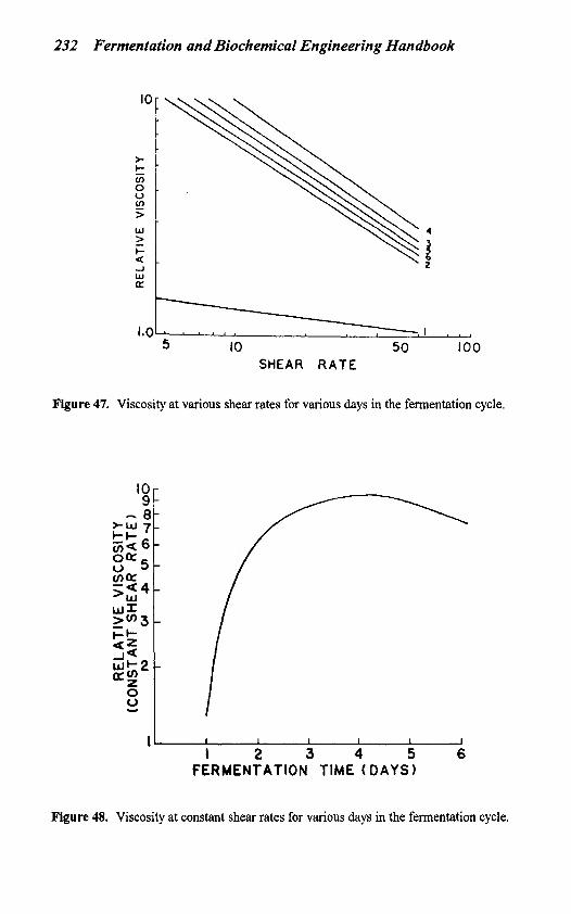
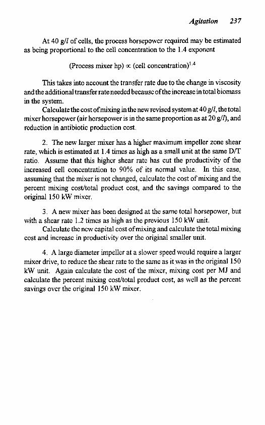
Within a given batch run, the cell concentration changes as a function of time. In addition, the viscosity goes up with cell concentration at a given point on the time curve of a fermenter. Figures 47 and 48 give typical data showing the change in viscosity as a function of the number of days of fermentation for different kinds of systems.
On the other hand, Fig. 49 shows the change in mass transfer rate with viscosity, which is caused largely by a change in cell concentration of the total process. It is true that the rate of oxygen transferred per MJ goes down as the cell concentration goes up. However, this cost must be balanced against the increasing productivity of a given dollar investment in fermentation tank, piping and total plant cost. Analysis needs to be made of the role that mixer cost, including both capital and power, plays in the total productivity cost in order to evaluate desirability of going in this direction.
A previous paper by Ryu and Oldshue treated an example where the final cell concentration was changed from 10 to 12 to 20 gll, and the oxygen mass transfer dropped from 10 to 8.3 to 6.4 mols oxygenh4J.
Looking at Table 4, the cost of electrical power and other essentials listed a capital cost of $900/kW (1982 cost about $2000/kW) if installed mixer capacity is used, including the associated blower and air supply, and including the installation of the equipment, with the electrical hookup. This is for a D/T ratio of 0.37.
232 Fermentation and Biochemical Engineering Handbook
SHEAR R A T E
Figure 47. Viscosity at various shear rates for various days in the fermentation cycle.
I I 2 3 4 5 6
FERMENTATION TIME ( D A Y S )
Figure 48. Viscosity at constant shear rates for various days in the fermentation cycle.
Agitation 233
CONSTANT H P t G A S
I I
I 10 100 R E L A T I V E VISCOSITY
Figure 49. Decrease in mass transfer rate with viscosity for a given mixer and air rate.
Table 4. Cost of Mixing for Production of Antibiotics (Based on Oxygen Transfer Rate)
Cost of electrical power Equipment Cost (expressed as power cost) Efficiency of oxygen mass transfer
Dilute system, lOg/l* More concentrated, 20gll*
Power and Equipment cost Cost of dissolved oxygen
10 glr 20 gll
Production cost of antibiotics Fractional cost for mixing
(antibiotics production) Production Yield
10 mols O,/MJ 6.4. mols O,/MJ l.St/MJ
0.15$/mol 0, 0.23#/mol 0, 46#fl<g
0.6-1.6%** 1 kgl200 mols 0,
*Cell concentration. **Of production cost.
234 Fermentation and Biochemical Engineering Handbook
Electrical power is assumed at 0.7$/MJ (to obtain $/kW-hour multiply by 3.6). The equipment is amortized, using present worth, over a 5-year period, which results in a figure of 0.8$/MJ. Total cost of the equipment and operation is therefore 1.5$/MJ. The cost of dissolving oxygen is 0.15$/mol 0, dissolved at 10 g/Z. At 20 g/Z, it is 0.23$/mol 0,.
Assuming that it takes 200 mols of oxygen to produce 1 kg of product and that there is a production cost of $60 total per kg of product, the percent cost of oxygen in the dilute system is approximately 0.7% of the total production cost. There is also assumed in this example that there is a fixed cost of $3Okg which does not change with the agitator, and that the variable fermentation cost goes down as the productivity of the particular tank in the process increased.
This is listed in Column A of Table 5 , Column D gives the results from the paper by Ryu and Oldshue, which described the use of a 500 hp mixer operating at 20g/Z. While the percent of cost due to the mixer has increased, the total production cost per kg of product has gone down 25% to a value of approximately $45.2/kg.
Table 5. Comparison of New Mixer to Original Mixer
transfer rate, g 0,llh 0.7 Maximum available oxygen
Fixed fermentation cost, $/kg 30 Variable ferm. cost, $/kg 30 Total production cost,
$/kg of product 60 Cost of oxygen transfer operation
(mixing equipment, power), $/kg 0.42
380 95
200 20
1 .o
1.1 30 15.2
45.2
0.52
380 380 380 95 95 95
180 200 200 20 20 20 0.9 1.0 1.0
1.1 1.1 1.1 30 30 30 16.67 15.16 15.34
46.7 45.16 45.34
0.57 0.58 0.72 Present cost of oxygen
transfer operation 0.7 1.1 1.2 1.3 1.6 Present cost savings - 25 22 25 24.5 Maximum impeller zone shear rate
(relative) 1 .oo 1.30 1.30 1.15 1.00
Agitation 235
Assume that this higher power mixer, having a maximum impeller zone shear rate 30% higher than Case A, decreased the growth ability of the microorganisms due to increased shear on these particles, changing the floc structure, etc. Further assume that th is cut the production ofpenicillin to 90% of the value it could have had based on cell concentration only. This means that the mixer is producing less product than Column D would indicate, and the production costs have gone up to $46.7/kg (Case E), because all the additional capacity of the larger aerator cannot be used. It can be seen that the aerator has given the ability to transfer 1.1 g 02/l/hr, in contrast to the 200 hp unit value of 0.7 g O,/l/hr.
Assume that studies in the laboratory indicate that if the shear rate is cutdown towhereitis only 15%higherthan CaseA,thentheorganismretains its growth potential. This mixer in Case F has a D/T ratio 40% higher and therefore, instead of $9OO/kW, costs $1200/kW, including the associated blower. Putting this into the cost example, even though it changes drastically the initial cost of the equipment, the productivity is improved to the point that the actual production cost is approximately $45.2/kg as it was in Case D.
If studies indicate that the shear rate has to be cut back to the same as it was in Case A, this means the mixer cost is now $1575/kW because of the increased torque and D/T, and it does raise the production cost up to $45.3 (Case G), but is still a very small percentage of the total production cost, and is a very small percentage in terms of mixer cost of the total production.
The main point here is that in this particular example, mixer horse- power and capital cost can effect tremendous changes in productivity because of their low cost in terms of the total cost.
9.0 SOME OTHER MASS TRANSFER CONSIDERATIONS
The desorption of CO, is an essential part of effective fermentation. The pressure and liquid depth that enhances absorption of oxygen discour- ages the desorption of CO,. Tall, thin tanks with the same volume of air, yielding a higher superficial velocity, normally give more pounds of oxygen transfer per total horsepower of mixer in air than do short, squat tanks. There also is less absorption of CO, under the same conditions. Therefore, some idea ofthe role of CO, desorption rates, back pressure of CO, and other things must be obtained in order to evaluate this particular phenomenon. In addition, the fluid mixing pattern in the fermenter must be considered. As broth becomes more viscous, and tanks become taller, more impellers are used and
236 Fermentation and Biochemical Engineering Handbook
there is a possibility of much longer top to bottom blending times being involved which do affect the dissolved C02-oxygen level throughout the system. In general, the dissolved C0,-oxygen level will assume some value intermediate between the values that would be predicted based on concentra- tion driving forces at the bottom and the top due to the gas stream.
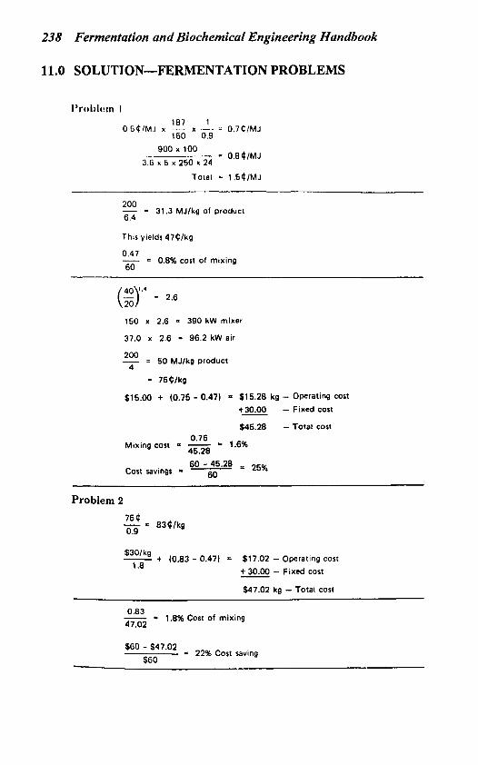
10.0 DESIGN PROBLEMS IN BIOCHEMICAL ENGINEERING
1. A mixer applying 150 kW to the mixer shaft is operating in a batch fermentation at a cell concentration of 20g/l. Associated with the mixer is a blower, which is providing air at a total expansion horsepower of 37 kW leaving the sparge ring. The cost of power is 0.5$/MJ. Use an overall energy efficiency for the equipment of 0.9.
The cost of the mixer plus the associated blower required, plus installation of both is $900/kW with an impeller diameter to tank diameter ratio of 0.35.
By using large diameter impellers at slower speeds, the maximum impeller zone fluid shear rate can be changed, and the cost of the mixerkW must be changed accordingly. The cost of the mixer can be approximated to change inversely proportional to the maximum impeller zone fluid shear rate to the 2.3 exponent
Cost cc (MIZSR)-2,3
The particular antibiotic requires 200 mols of oxygen for each kg of product produced. The total production cost ofthe antibiotic is estimated as $60/kg, of which $30 is a fixed cost, independent of productivity of the fermenter, and $30 is the cost associated with the actual fermentation tank itself.
At 20 g/1 cell concentration, the mixer is capable of transferring 6.4 mols of oxygen per MJ.
It is proposed to increase the solids concentration in the system to 40 g/l , which will effectively double the productivity of the fermentation tank itself. The oxygen transfer activity of the mixer is lowered, due to the increased viscosity, to 4 mol of oxygen per MJ.
Assuming that the mixer is operated for 250 days per year, and using a 5-year evaluation period, calculate the cost of mixing, capital and operating, in this process, and the percentage cost ofmixing under the present operation.
Agitation 23 7
At 40 gl1 of cells, the process horsepower required may be estimated as being proportional to the cell concentration to the 1.4 exponent
(Process mixer hp) oc (cell c~ncentration)'.~
This takes into account the transfer rate due to the change in viscosity and the additional transfer rate needed because ofthe increase in total biomass in the system.
Calculate the cost of mixing in the new revised system at 40 gll, the total mixer horsepower (air horsepower is in the same proportion as at 20 glZ), and reduction in antibiotic production cost.
2. The new larger mixer has a higher maximum impeller zone shear rate, which is estimated at 1.4 times as high as a small unit at the same D/T ratio. Assume that this higher shear rate has cut the productivity of the increased cell concentration to 90% of its normal value. In this case, assuming that the mixer is not changed, calculate the cost of mixing and the percent mixing cost/total product cost, and the savings compared to the original 15 0 kW mixer.
3. A new mixer has been designed at the same total horsepower, but
Calculate the new capital cost of mixing and calculate the total mixing with a shear rate 1.2 times as high as the previous 150 kW unit.
cost and increase in productivity over the original smaller unit.
4. A large diameter impeller at a slower speed would require a larger mixer drive, to reduce the shear rate to the same as it was in the original 150 kW unit. Again calculate the cost of the mixer, mixing cost per MJ and calculate the percent mixing cost/total product cost, as well as the percent savings over the original 150 kW mixer.
238 Fermentation and Biochemical Engineering Handbook
11.0 SOLUTION-FERMENTATION PROBLEMS
I'roblcin I 187 1
160 0.9 o . ~ C / M J x - x
900 x 100 3.6 x 6 x 260 x 24
Total
= 0.76/MJ
= O . ~ ( / M J
= l d $ / M J
200 _ = 31.3 MJ/kg 01 product 6.4
This yields 47(/kg
0.47 - = 0.8% cost of mixing 60
150 x 2.6 = 390 kW mixet
37.0 x 2.6 = 96.2 kW air
200 - = 50 MJ/kg product 4
= 75$/kg
$15.00 t (0.76 - 0.47) - $15.28 kg - Operating cost +E - Fixed cost
240 Fermentation and Biochemical Engineering Handbook
LIST OF ABBREVIATIONS
D KLa
&a
MJ N P P P* Q S.R. S.S. P W
F
K8
c'
c DO H K factor
z T O.U.R. MIZSR
d1 kwh kW CI kg
Impeller diameter Gas-liquid mass transfer coefficient based on
partial pressures Gas-liquid mass transfer coefficient based on liquid
concentrations Megajoule Impeller Power Pressure Equilibrium partial pressure Impeller pumping capacity Shear Rate Shear Stress Viscosity Width of square or rectangular tank
total air Superficial gas velocity, cross-section area of tank Liquid solid coefficient Equilibrium oxygen concentration corresponding to
partial pressure in air stream Liquid oxygen concentration Dissolved oxygen concentration Impeller head Ratio of horsepower with gas to power with gas off at
Liquid level Tank diameter Oxygen Uptake Rate Maximum impeller zone shear rate Grams per liter Kilowatt-hour Kilowatt Center Inlet gas introduction Kilogram
constant speed
Agitation 241
REFERENCES
1. 2.
3 .
4.
5 .
6 .
7.
Deindoerfer, F. H. and Gaden, E. L., Appl. Microbiol., 3:253 (1955) Oldshue, J. Y., FermentationMixing Scale-UpTechniques, Biotech, Bioeng.,
Oldshue, J. Y., Suspending Solids and Dispersing Gases inMixing Vessels, Ind. Eng. Chem., 61:79-89 (1969) Oldshue, J. Y., Spectrum of Fluid Shear Rates in Mixing Vessel, Chemeca '70 Australia, Butterworth (1970) Oldshue, J. Y., Coyle, C. K., and Connelly, G. L., Gas-Liquid Contacting with Impeller Mixers, Chem. Eng. Prog., 85-89 (March, 1977) Oldshue, J. Y., Coyle, C. K., et al., Fluid Mixing in the optimization of fermentation Production, Process Biochem., 13(1 l) , England 1978) Ryu, D. Y. and Oldshue, J. Y., A Reassessment of Mixing Costs in Fermentation Processes, Biotech. Bioeng., XX621-629 (1977)