Impact of local broadband turbidity estimation on forecastingof clear sky direct normal irradiance

Rich H. Inman, James G. Edson, Carlos F.M. Coimbra ⇑

Department of Mechanical and Aerospace Engineering, Jacobs School of Engineering, Center for Renewable Resource Integration and Center forEnergy Research, University of California, San Diego, La Jolla, CA 93093, USA

Received 25 March 2014; received in revised form 13 April 2015; accepted 26 April 2015Available online 16 May 2015

Communicated by: Associate Editor Christian A. Gueymard

Abstract

Clear-sky modeling is of critical importance for the accurate determination of Direct Normal Irradiance (DNI), which is the relevantcomponent of the solar irradiance for concentrated solar energy applications. Accurate clear-sky modeling of DNI is typically bestachieved through the separate consideration of water vapor and aerosol concentrations in the atmosphere. Highly resolved temporalmeasurements of such quantities is typically not available unless a meteorological station is located in close proximity. When this typeof data is not available, attenuating effects on the direct beam are modeled by Linke turbidity-equivalent factors, which can be obtainedfrom broadband observations of DNI under cloudless skies. We present a novel algorithm that allows for a time-resolved estimation ofthe average daily Linke turbidity factor from ground-based DNI observations under cloudless skies. This requires a method of identi-fying clear-sky periods in the observational time series (in order to avoid cloud contamination) as well as a broadband turbidity-basedclear-sky model for implicit turbidity calculations. While the method can be applied to the correction of historical clear-sky models for agiven site, the true value lies in the forecasting of DNI under cloudless skies through the assumption of a persistence of average dailyturbidity. This technique is applied at seven stations spread across the states of California, Washington, and Hawaii while using severalyears of data from 2010 to 2014. Performance of the forecast is evaluated by way of the relative Root Mean Square Error (rRMSE) andrelative Mean Bias Error (rMBE), both as a function of solar zenith angle, and benchmarked against monthly climatologies of turbidityinformation. Results suggest that rRMSE and rMBE of the method are typically smaller than 5% for both historical and forecastedCSMs, which compare favorably against the 10–20% range that is typical for monthly climatologies.! 2015 Elsevier Ltd. All rights reserved.

Keywords: Direct normal irradiance; Linke turbidity; Solar forecasting; Aerosols

1. Introduction

Knowledge of clear-sky irradiance plays a critical role inseveral solar engineering applications including the defini-tion of clear-sky indices, the development of smart persis-tence forecasts, the normalization of informationretrieved from satellite data, and the calculation of

forecasting skill metrics (Inman et al., 2013). In particular,clear-sky modeling is essential for the accurate determina-tion of Direct Normal Irradiance (DNI) under cloudlessskies. DNI is the critical component of the solar irradiancefor Concentrated Solar Power (CSP) applications such asthe recently completed Ivanpah Solar Electric GeneratingSystem located in the Mojave Desert of California, whichat the time of writing is the largest solar thermal projectin the world (392 MW). Although CSP technologies cur-rently represent only a small fraction of renewable energy

http://dx.doi.org/10.1016/j.solener.2015.04.0320038-092X/! 2015 Elsevier Ltd. All rights reserved.

⇑ Corresponding author.E-mail address: ccoimbra@ucsd.edu (C.F.M. Coimbra).

www.elsevier.com/locate/solener

Available online at www.sciencedirect.com

ScienceDirect

Solar Energy 117 (2015) 125–138

portfolios on a global scale, annual energy generated fromsuch technologies are expected to exceed 30 TW h by 2017(IEA, 2013).

Increased CSP market share will require further policyaction to tackle technical and financing challenges that cur-rently hinder deployment (IEA, 2014). One approach tolower the cost of grid integration is the application ofDNI/CSP forecasting, which makes CSP plants morefinancially attractive to deploy. These forecasts are usedto determine optimal operational strategies that maximizeprofit by minimizing penalty charges resulting from differ-ences between plant output and forecasted output. As aresult of CSP plants being driven by DNI, the determina-tion of such optimal operational strategies for CSP plantsdepends strongly on the accuracy of DNI forecasting. Ingeneral, forecast uncertainties are driven by variability incloud cover. However, it is well known that under cloudlessskies the presence of aerosol particles and water vaporbecome the most important factors influencing the inten-sity of ground level DNI (Gueymard, 2012a; Eltbaakhet al., 2012).

The term aerosol is used to describe either liquid or solidparticles that are suspended in the atmosphere with sizesranging from 1 to 105 nm in radius (Wen, 1996). Aerosolsin the atmosphere may be either natural or anthropogenicin origin and include particles such as fine soil, pollen, andmicroorganisms lifted by the wind; sea salts escaping frombreaking waves; smoke and soot emitted from fires; ashand dust erupting from volcanoes; sulfates created by theburning of coal and oil; and black carbon released duringthe incomplete combustion of heavy petroleum products.The net effect of aerosols on local microclimates dependon three primary mechanisms: direct radiative forcing asa result of scattering and absorption of visible and infraredradiation in the atmospheric boundary layer, indirectradiative forcing associated with changes in the microphys-ical and optical properties of cloud fields, and local heatingin the cloud formation layer due to highly absorbent aero-sols such as black carbon (Stefan et al., 2006). Although itis clear that DNI attenuation under cloudless skies is dri-ven by aerosol variability, the magnitude of these influ-ences is poorly constrained as a result of the highlyspatial–temporal variability of aerosol particles in theatmosphere as well as the fragmentary knowledge of theprocesses which control the physical, chemical, and opticalproperties of aerosol distributions (Morcrette et al., 2003;Kaskaoutis and Kambezidis, 2008; Chin et al., 2002).

Several methods for the quantification of atmosphericaerosol loading are available in the literature includingboth ground-based and remote sensing techniques (seeSection 2). While current satellites provide dailymulti-wavelength AOD data for nearly any location onthe planet, their quality is questionable at times as a resultof missing pixels in AOD retrievals and cloud contamina-tion. Ground-based pyrheliometers, on the other hand,are typically located at CSP sites and offer a highly resolvedtemporal signal of DNI, which under cloudless skies is

related to atmospheric aerosol loading. Therefore, highlytemporally resolved ground-based observations of DNIunder clear skies allow for a robust sampling of local tur-bidity, specifically at locations of interest to CSP plantoperators.

Several authors have examined the derivation of atmo-spheric aerosol loading from broadband irradiance mea-surements. More specifically, Louche et al. (1987)assigned a fixed value to the Angstrom exponent a (seeSection 2) and calculated the Angstrom turbidity coeffi-cient b from DNI observations over Ajaccio (France).Gueymard and Vignola (1998) developed asemi-empirical model that demonstrated the utility of thediffuse component of broadband irradiance for estimatingatmospheric turbidity. Canada et al. (1993) also assigneda fixed value to a in order to estimate b in Valencia(Spain) and compared the results with those fromAjaccia, Avignon, and Dhahran. Ineichen (2008) presenteda conversion function between T LI , the atmospheric watervapor and urban aerosol content that also accounts forthe altitude of the application site.

More recently, Polo et al. (2009) proposed a method toestimate daily Linke turbidity factor by using global irradi-ance measurements at solar noon. Gueymard (2013) pro-vided an efficient method to derive Aerosol OpticalDepth (AOD) information from broadband DNI measure-ments and addressed several critical issues including:instrument error, impact of model performance, propaga-tion of errors due to incorrect precipitable water, elimina-tion of cloudy conditions, and evaluation of a. Gueymard(2014) also evaluated the impact of on-site atmosphericwater vapor estimation methods on the accuracy of localsolar irradiance predictions. Bilbao et al. (2014), proposeda method for deriving Angstrom’s turbidity coefficient andthe AOD at 550 nm from broadband DNI observationsover Castilla y Leon (Spain), from July 2010 toDecember 2012.

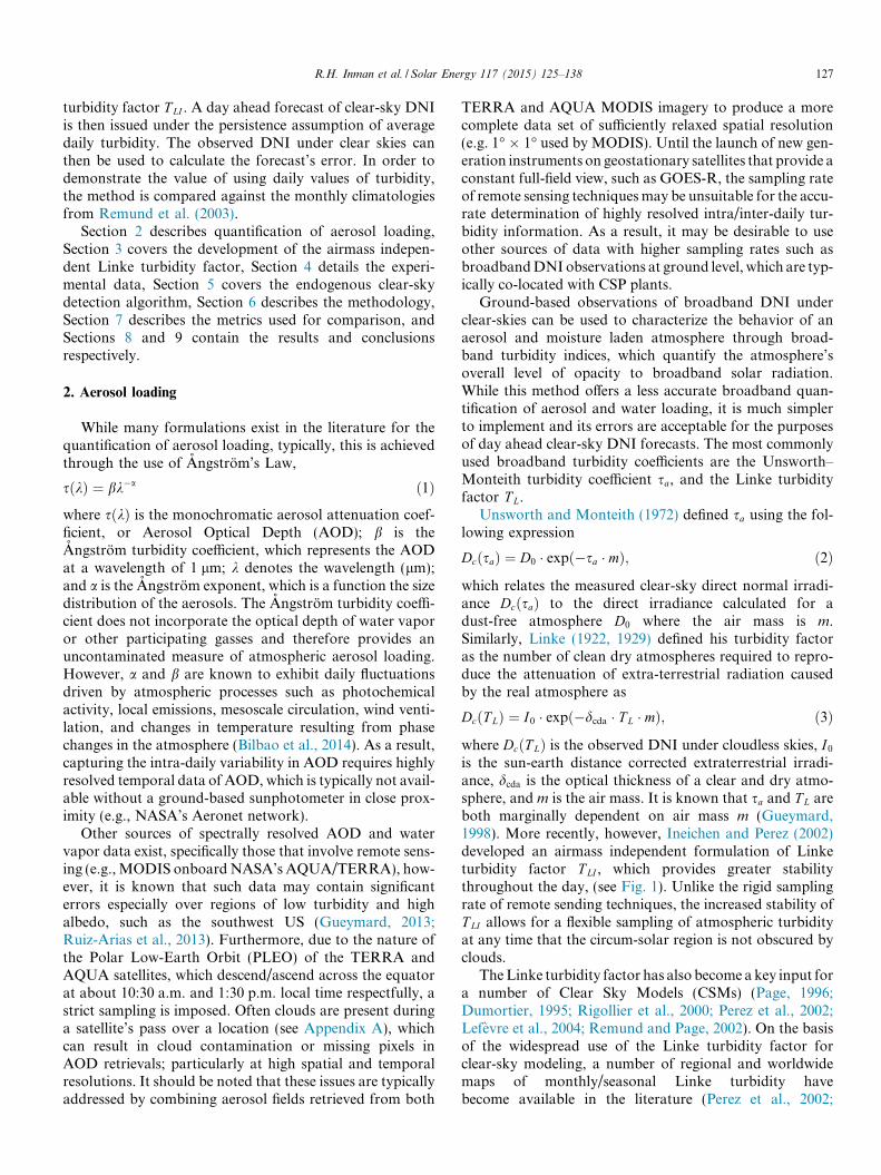
In addition to the implicit calculation of aerosol loadingfrom irradiance observations, detailed algorithms exist inthe literature that produce aerosol forecasts for aerosolfields using remote sensing techniques and transport mod-els, see for example Masmoudi et al. (2003). However, thiscontribution demonstrates the utility of ground-based esti-mations of average daily turbidity for the day-ahead fore-casting of broadband clear-sky DNI at a specific site.Because of CSP’s dependance on broadband DNI, thisirradiance component tends to be measured on site result-ing in readily available broadband turbidity information atsuch locations. An endogenous clear-sky detection algo-rithm for DNI is developed, which is based on the workof Reno et al. (2012), and applied to nearly ten site-yearsof data from seven stations spread across the states ofCalifornia, Washington, and Hawaii (see Fig. 3). Thesedata represent a number of widely varying microclimateswhich are used to speak to the robustness of the algorithm.Observations of clear-sky DNI are subsequently used tocalculate the daily average air mass independent Linke

126 R.H. Inman et al. / Solar Energy 117 (2015) 125–138

turbidity factor T LI . A day ahead forecast of clear-sky DNIis then issued under the persistence assumption of averagedaily turbidity. The observed DNI under clear skies canthen be used to calculate the forecast’s error. In order todemonstrate the value of using daily values of turbidity,the method is compared against the monthly climatologiesfrom Remund et al. (2003).

Section 2 describes quantification of aerosol loading,Section 3 covers the development of the airmass indepen-dent Linke turbidity factor, Section 4 details the experi-mental data, Section 5 covers the endogenous clear-skydetection algorithm, Section 6 describes the methodology,Section 7 describes the metrics used for comparison, andSections 8 and 9 contain the results and conclusionsrespectively.

2. Aerosol loading

While many formulations exist in the literature for thequantification of aerosol loading, typically, this is achievedthrough the use of Angstrom’s Law,

sðkÞ ¼ bk$a ð1Þ

where sðkÞ is the monochromatic aerosol attenuation coef-ficient, or Aerosol Optical Depth (AOD); b is theAngstrom turbidity coefficient, which represents the AODat a wavelength of 1 lm; k denotes the wavelength (lm);and a is the Angstrom exponent, which is a function the sizedistribution of the aerosols. The Angstrom turbidity coeffi-cient does not incorporate the optical depth of water vaporor other participating gasses and therefore provides anuncontaminated measure of atmospheric aerosol loading.However, a and b are known to exhibit daily fluctuationsdriven by atmospheric processes such as photochemicalactivity, local emissions, mesoscale circulation, wind venti-lation, and changes in temperature resulting from phasechanges in the atmosphere (Bilbao et al., 2014). As a result,capturing the intra-daily variability in AOD requires highlyresolved temporal data of AOD, which is typically not avail-able without a ground-based sunphotometer in close prox-imity (e.g., NASA’s Aeronet network).

Other sources of spectrally resolved AOD and watervapor data exist, specifically those that involve remote sens-ing (e.g., MODIS onboard NASA’s AQUA/TERRA), how-ever, it is known that such data may contain significanterrors especially over regions of low turbidity and highalbedo, such as the southwest US (Gueymard, 2013;Ruiz-Arias et al., 2013). Furthermore, due to the nature ofthe Polar Low-Earth Orbit (PLEO) of the TERRA andAQUA satellites, which descend/ascend across the equatorat about 10:30 a.m. and 1:30 p.m. local time respectfully, astrict sampling is imposed. Often clouds are present duringa satellite’s pass over a location (see Appendix A), whichcan result in cloud contamination or missing pixels inAOD retrievals; particularly at high spatial and temporalresolutions. It should be noted that these issues are typicallyaddressed by combining aerosol fields retrieved from both

TERRA and AQUA MODIS imagery to produce a morecomplete data set of sufficiently relaxed spatial resolution(e.g. 1" % 1" used by MODIS). Until the launch of new gen-eration instruments on geostationary satellites that provide aconstant full-field view, such as GOES-R, the sampling rateof remote sensing techniques may be unsuitable for the accu-rate determination of highly resolved intra/inter-daily tur-bidity information. As a result, it may be desirable to useother sources of data with higher sampling rates such asbroadband DNI observations at ground level, which are typ-ically co-located with CSP plants.

Ground-based observations of broadband DNI underclear-skies can be used to characterize the behavior of anaerosol and moisture laden atmosphere through broad-band turbidity indices, which quantify the atmosphere’soverall level of opacity to broadband solar radiation.While this method offers a less accurate broadband quan-tification of aerosol and water loading, it is much simplerto implement and its errors are acceptable for the purposesof day ahead clear-sky DNI forecasts. The most commonlyused broadband turbidity coefficients are the Unsworth–Monteith turbidity coefficient sa, and the Linke turbidityfactor T L.

Unsworth and Monteith (1972) defined sa using the fol-lowing expression

DcðsaÞ ¼ D0 & expð$sa & mÞ; ð2Þ

which relates the measured clear-sky direct normal irradi-ance DcðsaÞ to the direct irradiance calculated for adust-free atmosphere D0 where the air mass is m.Similarly, Linke (1922, 1929) defined his turbidity factoras the number of clean dry atmospheres required to repro-duce the attenuation of extra-terrestrial radiation causedby the real atmosphere as

DcðT LÞ ¼ I0 & expð$dcda & T L & mÞ; ð3Þ

where DcðT LÞ is the observed DNI under cloudless skies, I0

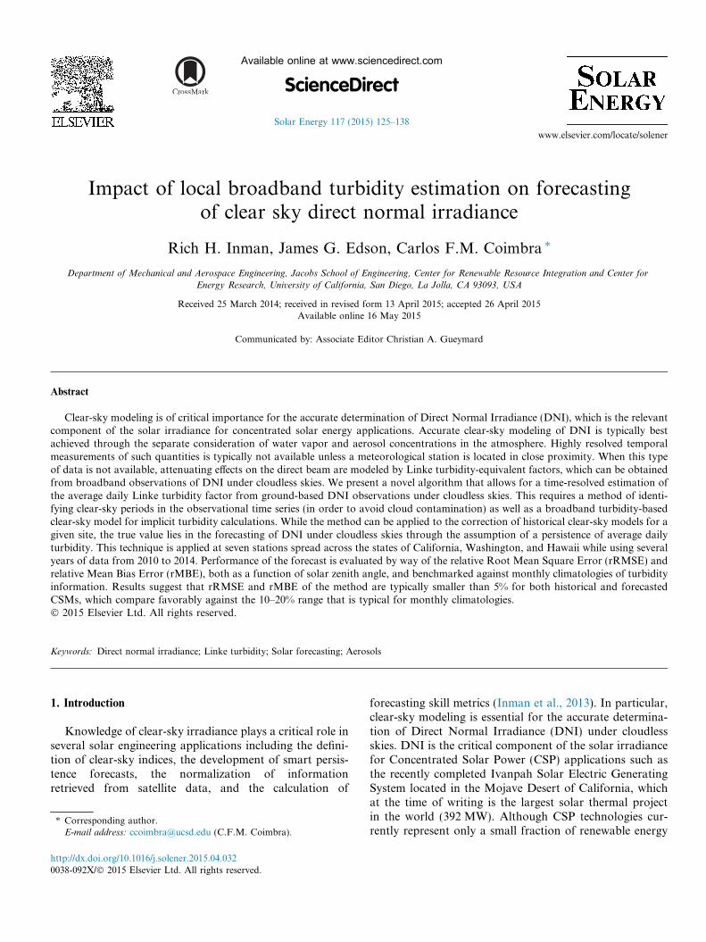
is the sun-earth distance corrected extraterrestrial irradi-ance, dcda is the optical thickness of a clear and dry atmo-sphere, and m is the air mass. It is known that sa and T L areboth marginally dependent on air mass m (Gueymard,1998). More recently, however, Ineichen and Perez (2002)developed an airmass independent formulation of Linketurbidity factor T LI , which provides greater stabilitythroughout the day, (see Fig. 1). Unlike the rigid samplingrate of remote sending techniques, the increased stability ofT LI allows for a flexible sampling of atmospheric turbidityat any time that the circum-solar region is not obscured byclouds.

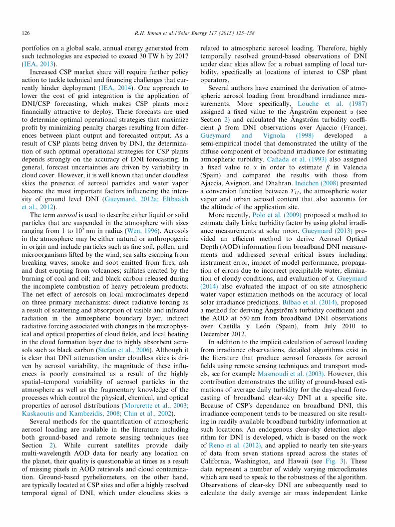
The Linke turbidity factor has also become a key input fora number of Clear Sky Models (CSMs) (Page, 1996;Dumortier, 1995; Rigollier et al., 2000; Perez et al., 2002;Lefevre et al., 2004; Remund and Page, 2002). On the basisof the widespread use of the Linke turbidity factor forclear-sky modeling, a number of regional and worldwidemaps of monthly/seasonal Linke turbidity havebecome available in the literature (Perez et al., 2002;

R.H. Inman et al. / Solar Energy 117 (2015) 125–138 127

Remund et al., 2003), an example of which is shown in Fig. 2.While the monthly/seasonal resolution of these maps areconvenient for locations where no ground truth exists andare typically sufficient for the clear-sky modeling of GHI(Reno et al., 2012), they are not suitable for the accuratemodeling of DNI, which demonstrates an increased sensitiv-ity to variability in aerosol loading.

In general, the scattering caused by aerosols undercloudless skies increases the local Diffuse HorizontalIrradiance (DHI) and commensurately decreases theDNI. This exchange between DHI and DNI effectively buf-fers the impact of aerosols on clear-sky Global HorizontalIrradiance (GHI), which can be seen in the closureequation,

G ¼ D cos hz þ d; ð4Þ

where the global horizontal irradiance G is defined as thegeometric sum of the direct normal irradiance D and dif-fuse horizontal irradiance d, and hz is the solar zenith angle.This buffering is the reason aerosol loading is known toattenuate DNI in the range of 30–100% as opposed toGHI where the attenuation is significantly lower at approx-imately 10% (Schroedter-Homscheidt and Oumbe, 2013;

Lara-Danego et al., 2012; Marquez and Coimbra, 2011).Furthermore, Gueymard (2012b) showed that DNI exhi-bits an Aerosol Sensitivity Index (ASI), which relates themagnitude of relative variations in irradiance to absolutevariations in aerosol optical depth, that is 2–4 times greaterthan that for GHI. The difference in intensity reductionbetween GHI and DNI is one key reason why GHI fore-casting techniques, which have been reviewed extensiveyin the literature (Gueymard, 2012a; Reno et al., 2012;

1,000

900

800

700

600

Irra

dian

ce [W

m-2

]

3.6

3.2

2.8

2.4

2.0

8 10 12 14 16

DNI

TLK

TLI

TL

Solar Time [h]

AM =

2

AM = 2

TLI @ AM = 2

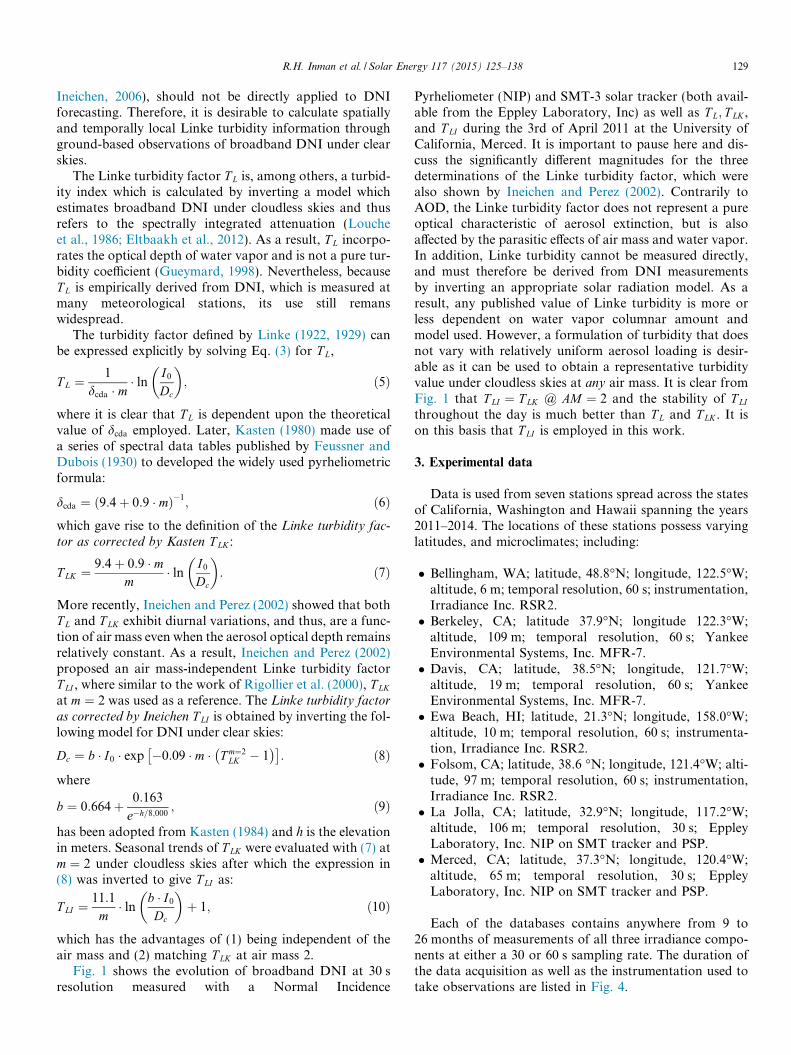
Fig. 1. Evolution of broadband Direct Normal Irradiance (DNI) at 30 sresolution measured with a Normal Incidence Pyrheliometer (NIP) andSMT-3 solar tracker (available from the Eppley Laboratory, Inc) as wellas T L; T LK , and T LI during the 3rd of April 2011 at the University ofCalifornia, Merced.

Fig. 2. Example of one of the monthly maps of Linke turbidity for the world developed by Remund et al. (2003). The maps can be downloaded from eitherthe Solar Radiation Data website (SoDa, 2014) or the HelioClim website (HelioClim, 2014).

Bellingham

Berkeley

La Jolla

Davis Folsom

Merced

Ewa Beach

Hawaii100m

Fig. 3. Map of the relative locations of the stations used in this study.

128 R.H. Inman et al. / Solar Energy 117 (2015) 125–138

Ineichen, 2006), should not be directly applied to DNIforecasting. Therefore, it is desirable to calculate spatiallyand temporally local Linke turbidity information throughground-based observations of broadband DNI under clearskies.

The Linke turbidity factor T L is, among others, a turbid-ity index which is calculated by inverting a model whichestimates broadband DNI under cloudless skies and thusrefers to the spectrally integrated attenuation (Loucheet al., 1986; Eltbaakh et al., 2012). As a result, T L incorpo-rates the optical depth of water vapor and is not a pure tur-bidity coefficient (Gueymard, 1998). Nevertheless, becauseT L is empirically derived from DNI, which is measured atmany meteorological stations, its use still remanswidespread.

The turbidity factor defined by Linke (1922, 1929) canbe expressed explicitly by solving Eq. (3) for T L,

T L ¼1

dcda & m& ln I0

Dc

! "; ð5Þ

where it is clear that T L is dependent upon the theoreticalvalue of dcda employed. Later, Kasten (1980) made use ofa series of spectral data tables published by Feussner andDubois (1930) to developed the widely used pyrheliometricformula:

dcda ¼ ð9:4þ 0:9 & mÞ$1; ð6Þ

which gave rise to the definition of the Linke turbidity fac-tor as corrected by Kasten T LK :

T LK ¼9:4þ 0:9 & m

m& ln I0

Dc

! ": ð7Þ

More recently, Ineichen and Perez (2002) showed that bothT L and T LK exhibit diurnal variations, and thus, are a func-tion of air mass even when the aerosol optical depth remainsrelatively constant. As a result, Ineichen and Perez (2002)proposed an air mass-independent Linke turbidity factorT LI , where similar to the work of Rigollier et al. (2000), T LK

at m ¼ 2 was used as a reference. The Linke turbidity factoras corrected by Ineichen T LI is obtained by inverting the fol-lowing model for DNI under clear skies:

Dc ¼ b & I0 & exp $0:09 & m & T m¼2LK $ 1

# $% &: ð8Þ

where

b ¼ 0:664þ 0:163

e$h=8;000; ð9Þ

has been adopted from Kasten (1984) and h is the elevationin meters. Seasonal trends of T LK were evaluated with (7) atm ¼ 2 under cloudless skies after which the expression in(8) was inverted to give T LI as:

T LI ¼11:1

m& ln b & I0

Dc

! "þ 1; ð10Þ

which has the advantages of (1) being independent of theair mass and (2) matching T LK at air mass 2.

Fig. 1 shows the evolution of broadband DNI at 30 sresolution measured with a Normal Incidence

Pyrheliometer (NIP) and SMT-3 solar tracker (both avail-able from the Eppley Laboratory, Inc) as well as T L; T LK ,and T LI during the 3rd of April 2011 at the University ofCalifornia, Merced. It is important to pause here and dis-cuss the significantly different magnitudes for the threedeterminations of the Linke turbidity factor, which werealso shown by Ineichen and Perez (2002). Contrarily toAOD, the Linke turbidity factor does not represent a pureoptical characteristic of aerosol extinction, but is alsoaffected by the parasitic effects of air mass and water vapor.In addition, Linke turbidity cannot be measured directly,and must therefore be derived from DNI measurementsby inverting an appropriate solar radiation model. As aresult, any published value of Linke turbidity is more orless dependent on water vapor columnar amount andmodel used. However, a formulation of turbidity that doesnot vary with relatively uniform aerosol loading is desir-able as it can be used to obtain a representative turbidityvalue under cloudless skies at any air mass. It is clear fromFig. 1 that T LI ¼ T LK @ AM ¼ 2 and the stability of T LI

throughout the day is much better than T L and T LK . It ison this basis that T LI is employed in this work.

3. Experimental data

Data is used from seven stations spread across the statesof California, Washington and Hawaii spanning the years2011–2014. The locations of these stations possess varyinglatitudes, and microclimates; including:

( Bellingham, WA; latitude, 48.8"N; longitude, 122.5"W;altitude, 6 m; temporal resolution, 60 s; instrumentation,Irradiance Inc. RSR2.( Berkeley, CA; latitude 37.9"N; longitude 122.3"W;

altitude, 109 m; temporal resolution, 60 s; YankeeEnvironmental Systems, Inc. MFR-7.( Davis, CA; latitude, 38.5"N; longitude, 121.7"W;

altitude, 19 m; temporal resolution, 60 s; YankeeEnvironmental Systems, Inc. MFR-7.( Ewa Beach, HI; latitude, 21.3"N; longitude, 158.0"W;

altitude, 10 m; temporal resolution, 60 s; instrumenta-tion, Irradiance Inc. RSR2.( Folsom, CA; latitude, 38.6 "N; longitude, 121.4"W; alti-

tude, 97 m; temporal resolution, 60 s; instrumentation,Irradiance Inc. RSR2.( La Jolla, CA; latitude, 32.9"N; longitude, 117.2"W;

altitude, 106 m; temporal resolution, 30 s; EppleyLaboratory, Inc. NIP on SMT tracker and PSP.( Merced, CA; latitude, 37.3"N; longitude, 120.4"W;

altitude, 65 m; temporal resolution, 30 s; EppleyLaboratory, Inc. NIP on SMT tracker and PSP.

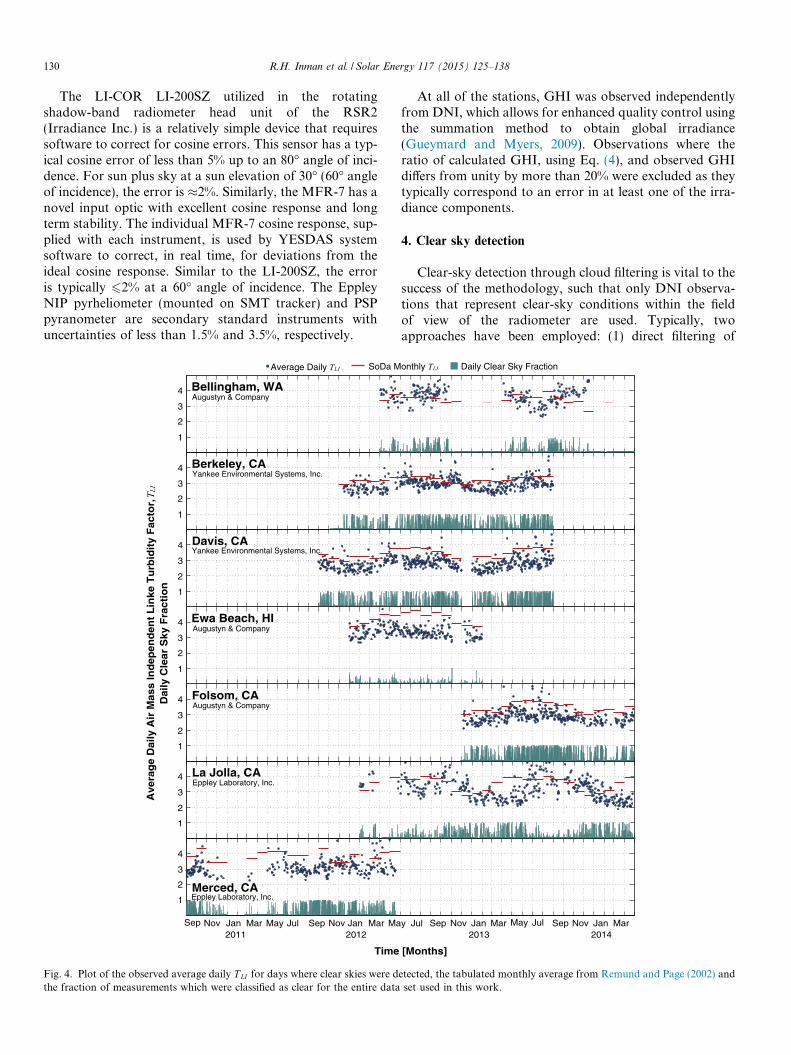
Each of the databases contains anywhere from 9 to26 months of measurements of all three irradiance compo-nents at either a 30 or 60 s sampling rate. The duration ofthe data acquisition as well as the instrumentation used totake observations are listed in Fig. 4.

R.H. Inman et al. / Solar Energy 117 (2015) 125–138 129

The LI-COR LI-200SZ utilized in the rotatingshadow-band radiometer head unit of the RSR2(Irradiance Inc.) is a relatively simple device that requiressoftware to correct for cosine errors. This sensor has a typ-ical cosine error of less than 5% up to an 80" angle of inci-dence. For sun plus sky at a sun elevation of 30" (60" angleof incidence), the error is )2%. Similarly, the MFR-7 has anovel input optic with excellent cosine response and longterm stability. The individual MFR-7 cosine response, sup-plied with each instrument, is used by YESDAS systemsoftware to correct, in real time, for deviations from theideal cosine response. Similar to the LI-200SZ, the erroris typically 62% at a 60" angle of incidence. The EppleyNIP pyrheliometer (mounted on SMT tracker) and PSPpyranometer are secondary standard instruments withuncertainties of less than 1.5% and 3.5%, respectively.

At all of the stations, GHI was observed independentlyfrom DNI, which allows for enhanced quality control usingthe summation method to obtain global irradiance(Gueymard and Myers, 2009). Observations where theratio of calculated GHI, using Eq. (4), and observed GHIdiffers from unity by more than 20% were excluded as theytypically correspond to an error in at least one of the irra-diance components.

4. Clear sky detection

Clear-sky detection through cloud filtering is vital to thesuccess of the methodology, such that only DNI observa-tions that represent clear-sky conditions within the fieldof view of the radiometer are used. Typically, twoapproaches have been employed: (1) direct filtering of

Davis, CA

1

2

3

4

1

2

3

4

1

2

3

4

1

2

3

4

1

2

3

4

1

2

3

4

1

2

3

4

Ave

rag

e D

aily

Air

Mas

s In

dep

end

ent

Lin

ke T

urb

idit

y F

acto

r, T LI

Dai

ly C

lear

Sky

Fra

ctio

n

Sep Nov Jan Mar May Jul Sep Nov Jan Mar May Jul Sep Nov Jan Mar May Jul2011 2012 2013

Time [Months]

Average Daily TLI SoDa Monthly TLI Daily Clear Sky Fraction

Bellingham, WA

Berkeley, CA

Ewa Beach, HI

Folsom, CA

La Jolla, CA

Merced, CA

Yankee Environmental Systems, Inc.

Augustyn & Company

Eppley Laboratory, Inc.

Yankee Environmental Systems, Inc.

Eppley Laboratory, Inc.

Augustyn & Company

Augustyn & Company

Sep Nov Jan Mar2014

Fig. 4. Plot of the observed average daily T LI for days where clear skies were detected, the tabulated monthly average from Remund and Page (2002) andthe fraction of measurements which were classified as clear for the entire data set used in this work.

130 R.H. Inman et al. / Solar Energy 117 (2015) 125–138

cloud conditions in the DNI time-series or (2) back-end fil-tering where all DNI data is used and observations thatprovide physically un-reasonable clear-sky conditions areeliminated.

The first approach has been implemented by Long andAckerman (2000), however, the Fortran files and executa-bles of the algorithm have been found to be slow and cum-bersome to use (Gueymard, 2013). The second approachwas adopted by AERONET for cloud-screening from sun-photometric observations (Smirnov et al., 2000) and morerecently Gueymard (2013) employed a similar techniquebased on five independent requirements.

In this work, rather than directly implement the Longfilter or adopt a back-end filtering, clear-sky detection isperformed using an endogenous statistical model whichwas originally developed by Reno et al. (2012) for GHIobservations. This method uses five criteria to compare atime period containing N observations of GHI to a corre-sponding CSM for the same period. The time period isdeemed “clear” if threshold values (whose values vary withN) for each criteria are met.

In this work, the criteria include the mean value of irra-diance I (global and direct) during the time period,

G ¼ 1

N

XN

t¼1

IðtÞ; ð11Þ

the maximum irradiance value M in the time series,

M ¼ max½IðtÞ+ 8 t 2 f1; 2; . . . ;Ng; ð12Þ

the length L of the line connecting the points in the timeseries that, unlike the L defined in Reno et al. (2012), doesnot account for the length of the time-step,

L ¼XN

t¼1

ffiffiffiffiffiffiffiffiffiffiffiffiffiffiffiffiffiffiffiffiffiffiffiffiffiffiffiffiffiffiffiffiffiffiffi½Iðt þ DtÞ $ IðtÞ+2

q; ð13Þ

the variance of changes in the time series; specifically, thenormalized standard deviation r of the slope betweensequential points,

r ¼

ffiffiffiffiffiffiffiffiffiffiffiffiffiffiffiffiffiffiffiffiffiffiffiffiffiffiffiffiffiffiffiffiffiffiffiffiffiffiffi1

N$1

PN$1t¼1 ðsðtÞ $ sÞ2

q

1N

PNt¼1IðtÞ

ð14Þ

where

sðtÞ ¼ Iðt þ DtÞ $ IðtÞ; 8 t 2 f1; 2; . . . ;Ng ð15Þ

s ¼ 1

N $ 1

XN$1

t¼1

sðtÞ ð16Þ

and, S the maximum deviation from the clear-sky slope sc,

S ¼ maxfjsðtÞ $ scðtÞjg 8 t 2 f1; 2; . . . ;Ng ð17Þ

where

scðtÞ ¼ Icðt þ DtÞ $ IcðtÞ: ð18ÞSimilar to Reno et al. (2012), in this work a 10-min slidingwindow is employed to determine if an observation is identi-fied as “clear”. The five clear-sky criteria (G;M ; L; r; and S)are evaluated for both the CSM and observational time

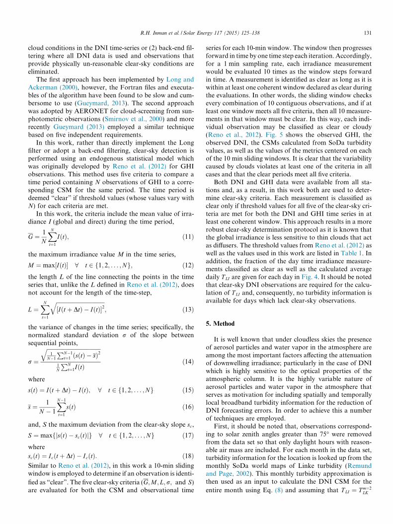
series for each 10-min window. The window then progressesforward in time by one time step each iteration. Accordingly,for a 1 min sampling rate, each irradiance measurementwould be evaluated 10 times as the window steps forwardin time. A measurement is identified as clear as long as it iswithin at least one coherent window declared as clear duringthe evaluations. In other words, the sliding window checksevery combination of 10 contiguous observations, and if atleast one window meets all five criteria, then all 10 measure-ments in that window must be clear. In this way, each indi-vidual observation may be classified as clear or cloudy(Reno et al., 2012). Fig. 5 shows the observed GHI, theobserved DNI, the CSMs calculated from SoDa turbidityvalues, as well as the values of the metrics centered on eachof the 10 min sliding windows. It is clear that the variabilitycaused by clouds violates at least one of the criteria in allcases and that the clear periods meet all five criteria.

Both DNI and GHI data were available from all sta-tions and, as a result, in this work both are used to deter-mine clear-sky criteria. Each measurement is classified asclear only if threshold values for all five of the clear-sky cri-teria are met for both the DNI and GHI time series in atleast one coherent window. This approach results in a morerobust clear-sky determination protocol as it is known thatthe global irradiance is less sensitive to thin clouds that actas diffusers. The threshold values from Reno et al. (2012) aswell as the values used in this work are listed in Table 1. Inaddition, the fraction of the day time irradiance measure-ments classified as clear as well as the calculated averagedaily T LI are given for each day in Fig. 4. It should be notedthat clear-sky DNI observations are required for the calcu-lation of T LI and, consequently, no turbidity information isavailable for days which lack clear-sky observations.

5. Method

It is well known that under cloudless skies the presenceof aerosol particles and water vapor in the atmosphere areamong the most important factors affecting the attenuationof downwelling irradiance; particularly in the case of DNIwhich is highly sensitive to the optical properties of theatmospheric column. It is the highly variable nature ofaerosol particles and water vapor in the atmosphere thatserves as motivation for including spatially and temporallylocal broadband turbidity information for the reduction ofDNI forecasting errors. In order to achieve this a numberof techniques are employed.

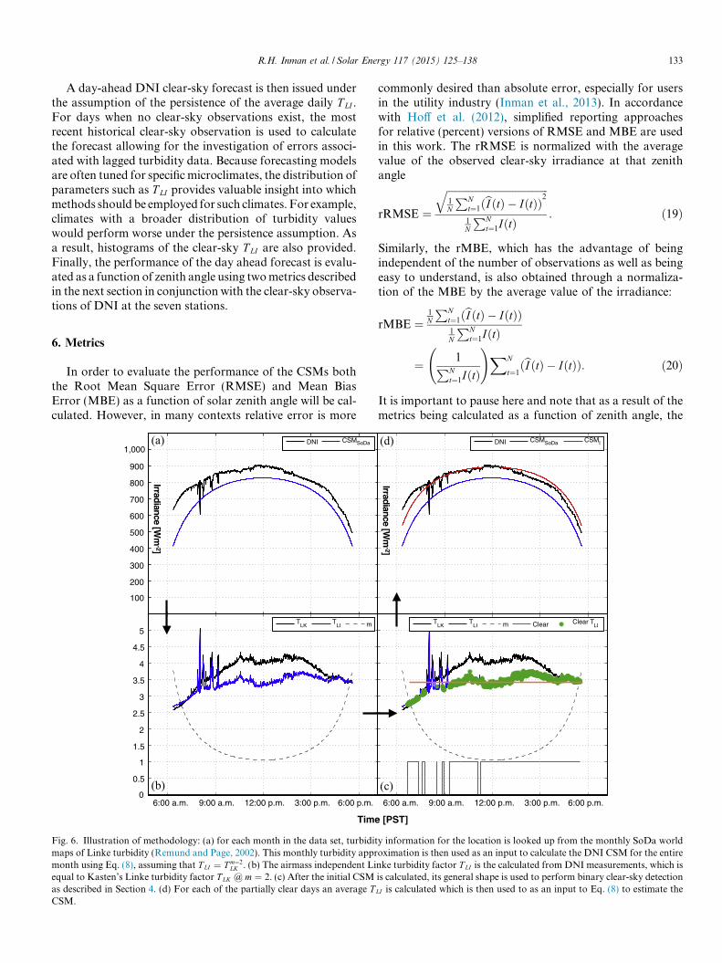
First, it should be noted that, observations correspond-ing to solar zenith angles greater than 75" were removedfrom the data set so that only daylight hours with reason-able air mass are included. For each month in the data set,turbidity information for the location is looked up from themonthly SoDa world maps of Linke turbidity (Remundand Page, 2002). This monthly turbidity approximation isthen used as an input to calculate the DNI CSM for theentire month using Eq. (8) and assuming that T LI ¼ T m¼2

LK

R.H. Inman et al. / Solar Energy 117 (2015) 125–138 131

as well as the GHI CSM from Ineichen and Perez (2002),see Fig. 6(a). The airmass independent Linke turbidity fac-tor T LI is the calculated from DNI measurements, which isequal to Kasten’s Linke turbidity factor T LK @ m ¼ 2, seeFig. 6(b). After this initial CSM and T LI are calculated, itsgeneral shape is used to perform a binary clear-sky detec-tion as described in Section 4, see Fig. 6(c). For each ofthe partially clear days an average T LI is calculated whichis then used to as an input to Eq. (8) to re-calculate theCSM, see Fig. 6(d). Each of the average daily T LI is shownin Fig. 4 for days where clear-sky observations exist.

1000

800

600

400

200

1000

800

600

400

200

1000

800

600

400

200

1000

800

600

400

200

1000

800

600

400

200

0

Irra

dian

ce

-2]

250

200

150

100

50

250

200

150

100

50

106

102

100

10-2

104

101

10-1

10-2

10 -3

100

10-1

10-1

∆G

| ∆M

||∆

L|| ∆

σ|| ∆

S|

Ground Truth MetricCSM

9:00 a.m. 12:00 p.m. 3:00 p.m. 9:00 a.m. 12:00 p.m. 3:00 p.m.

Time [PST]

GHI

GHI

GHI

GHI

GHI

DNI

DNI

DNI

DNI

DNI

June 2, 2012 - Berkeley, CA

Fig. 5. Observed GHI and DNI, the CSMs calculated from persistence turbidity values, as well as the value of them metric centered at the 10 min slidingwindow. It is clear that the variability caused by clouds violates at least one of the criteria in all cases and that the clear periods meet all five criteria.

Table 1Clear sky criteria threshold values from Reno et al. (2012) (GHIReno) aswell as the values used in this work (GHIInman and DNIInman). Thethresholds for DNI were slightly relaxed as a result of increased variabilityin the observational DNI time series.

GHIReno GHIInman DNIInman

G ,75W m$2 ,100 W m$2 ,200 W m$2

M ,75 W m$2 ,100 W m$2 ,200 W m$2

L $5 to 10 ,50 ,100r < 0:005 < 0:01 < 0:015S < 8 W m$2 < 10 W m$2 < 15 W m$2

132 R.H. Inman et al. / Solar Energy 117 (2015) 125–138

A day-ahead DNI clear-sky forecast is then issued underthe assumption of the persistence of the average daily T LI .For days when no clear-sky observations exist, the mostrecent historical clear-sky observation is used to calculatethe forecast allowing for the investigation of errors associ-ated with lagged turbidity data. Because forecasting modelsare often tuned for specific microclimates, the distribution ofparameters such as T LI provides valuable insight into whichmethods should be employed for such climates. For example,climates with a broader distribution of turbidity valueswould perform worse under the persistence assumption. Asa result, histograms of the clear-sky T LI are also provided.Finally, the performance of the day ahead forecast is evalu-ated as a function of zenith angle using two metrics describedin the next section in conjunction with the clear-sky observa-tions of DNI at the seven stations.

6. Metrics

In order to evaluate the performance of the CSMs boththe Root Mean Square Error (RMSE) and Mean BiasError (MBE) as a function of solar zenith angle will be cal-culated. However, in many contexts relative error is more

commonly desired than absolute error, especially for usersin the utility industry (Inman et al., 2013). In accordancewith Hoff et al. (2012), simplified reporting approachesfor relative (percent) versions of RMSE and MBE are usedin this work. The rRMSE is normalized with the averagevalue of the observed clear-sky irradiance at that zenithangle

rRMSE ¼

ffiffiffiffiffiffiffiffiffiffiffiffiffiffiffiffiffiffiffiffiffiffiffiffiffiffiffiffiffiffiffiffiffiffiffiffiffiffiffiffi1N

PNt¼1ðbI ðtÞ $ IðtÞÞ

2q

1N

PNt¼1IðtÞ

: ð19Þ

Similarly, the rMBE, which has the advantage of beingindependent of the number of observations as well as beingeasy to understand, is also obtained through a normaliza-tion of the MBE by the average value of the irradiance:

rMBE ¼1N

PNt¼1ðbI ðtÞ $ IðtÞÞ1N

PNt¼1IðtÞ

¼ 1PN

t¼1IðtÞ

!XN

t¼1ðbI ðtÞ $ IðtÞÞ: ð20Þ

It is important to pause here and note that as a result of themetrics being calculated as a function of zenith angle, the

DNI CSMSoDa

TLK

TLI m T

LKT

LI m Clear Clear TLI

DNI CSMSoDa CSMI(a)

(b) (c)

(d)

6:00 a.m. 12:00 p.m. 6:00 p.m.9:00 a.m. 3:00 p.m. 6:00 a.m. 12:00 p.m. 6:00 p.m.9:00 a.m. 3:00 p.m.

Time [PST]

0

0.5

1

1.5

2

2.5

3

3.5

4

4.5

5

100

200

300

400

500

600

700

800

900

1,000

Irradiance [Wm

-2]

Irradiance [Wm

-2]

Fig. 6. Illustration of methodology: (a) for each month in the data set, turbidity information for the location is looked up from the monthly SoDa worldmaps of Linke turbidity (Remund and Page, 2002). This monthly turbidity approximation is then used as an input to calculate the DNI CSM for the entiremonth using Eq. (8), assuming that T LI ¼ T m¼2

LK . (b) The airmass independent Linke turbidity factor T LI is the calculated from DNI measurements, which isequal to Kasten’s Linke turbidity factor T LK @ m ¼ 2. (c) After the initial CSM is calculated, its general shape is used to perform binary clear-sky detectionas described in Section 4. (d) For each of the partially clear days an average T LI is calculated which is then used to as an input to Eq. (8) to estimate theCSM.

R.H. Inman et al. / Solar Energy 117 (2015) 125–138 133

average value in (19) and (20) correspond to the averagevalue at a given zenith angle, rather than the average valueover the entire time series. Furthermore, as a point of clar-ification, observations were separated in bins of equalzenith angle rounded to the nearest degree, prior to the cal-culation of the metrics at each zenith angle. While thiscomes with an additional computational expense, the

impact is insignificant compared to the implementation ofthe method itself.

7. Results

As mentioned in Section 5, the calculated average dailyT LI for days with clear-sky observations, the monthly SoDaT LI , and the fraction of each day that was classified as clearusing the method described in Section 4 are shown inFig. 4. Fig. 4 illustrates that, with the exception ofBellingham and La Jolla, the calculated average daily T LI

for all stations was typically 15–30% less than the monthlySoDa values for T LI indicating that the SoDa database forT LI tends to underestimate DNI for the particular CSMemployed in this work. It is also clear from Fig. 4 thatFolsom, Davis, Merced and Berkeley (all located within-160 km from each other) were characterized by a largefraction of clear days. The remaining sites exhibited signif-icantly fewer clear-sky observations with tropical EwaBeach, HI, showing the fewest followed by Bellingham,

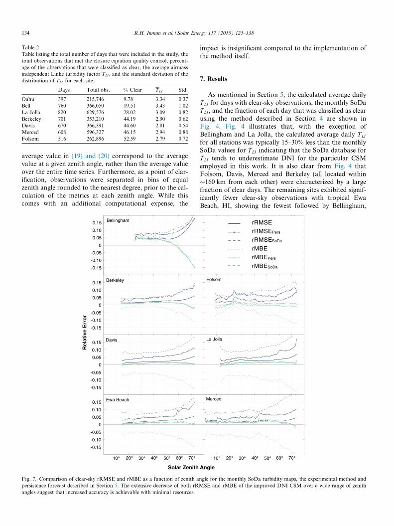
Table 2Table listing the total number of days that were included in the study, thetotal observations that met the closure equation quality control, percent-age of the observations that were classified as clear, the average airmassindependent Linke turbidity factor T LI , and the standard deviation of thedistribution of T LI for each site.

Days Total obs. % Clear T LI Std.

Oahu 397 215,746 9.78 3.34 0.37Bell 760 366,050 19.51 3.43 1.02La Jolla 820 629,576 28.02 3.09 0.82Berkeley 701 353,210 44.19 2.90 0.62Davis 670 366,391 44.60 2.81 0.54Merced 608 596,327 46.15 2.94 0.88Folsom 516 262,896 52.59 2.79 0.72

rRMSErRMSEPers

rRMSESoDa

rMBErMBEPers

rMBESoDa

0

0.05

0.10

-0.05

-0.10

-0.15

Rel

ativ

e E

rror

Solar Zenith Angle

Bellingham

Berkeley

Davis

Ewa Beach

Folsom

La Jolla

Merced

0.15

0.05

0.10

-0.05

-0.10

-0.15

0.15

0.05

0.10

-0.05

-0.10

-0.15

0.15

0.05

0.10

-0.05

-0.10

-0.15

0.15

0

0

0

Fig. 7. Comparison of clear-sky rRMSE and rMBE as a function of zenith angle for the monthly SoDa turbidity maps, the experimental method andpersistence forecast described in Section 5. The extensive decrease of both rRMSE and rMBE of the improved DNI CSM over a wide range of zenithangles suggest that increased accuracy is achievable with minimal resources.

134 R.H. Inman et al. / Solar Energy 117 (2015) 125–138

which is consistently overcast, and coastal La Jolla, with itsvolatile marine layer. Table 2 lists the total number of daysthat were included in the study, the total observations thatmet the closure equation quality control, percentage of theobservations that were classified as clear, the average air-mass independent Linke turbidity factor, and the standarddeviation of the T LI distribution for each site.

The relative (or percent) versions of the RMSE andMBE described in Section 6 were also calculated as a func-tion of solar zenith angle in this work. Again, we comparethe CSM obtained from the monthly SoDa maps of T LI

with the experimental method and persistence forecastdescribed in Section 5. The statistics are based on dayswhere at least 10% of the observations are clear in orderto ensure an accurate sampling of the attenuation causedby the atmospheric column. Overall, this set of validationmetrics is presented in Fig. 7. The rRMSE for the methodapplied to the same day is typically less than 5% and can beas low as 0.5% for zenith angles less than 30"; with theexception of Bellingham, WA whose rRMSE exceeds 5%for zenith angles greater than 60". The rRMSEPers of theforecasted persistence T LI CSM had a similar shape tothe rRMSE with an additional 1–3% error while themonthly SoDa T LI produced an rRMSESoDa of a compara-ble shape with an additional 3–5% error over therRMSEPers.

Fig. 7 also shows that the rMBE of the monthly SoDaT LI is consistently negative for all zenith angles, which isalso in agreement with the results presented in Fig. 4 and

again suggests that the SoDa input data in conjunctionwith the CSM employed in this work consistently underes-timates DNI through an overestimation of T LI . It should benoted that the rMBEPers was similar to the rMBE of theimproved CSM for all of the sites, including Bellingham,WA. The relatively small (-1–2%) and positive rMBE ofthe improved and forecasted CSMs also indicate a slightover estimation of DNI rather than the notable underesti-mation provided by the monthly SoDa T LI data, which istypically desirable of CSMs.

Finally, Fig. (8) shows the histograms of the averagedaily T LI for each of the seven stations. It is clear that, withthe exception of Bellingham and La Jolla, a general trend isapparent in the distribution of T LI . Most of the sites exhibitan almost normal distribution centered near T LI ¼ 3.Bellingham, however has a distribution which is shiftedto the right and centered near 3.75. This value is character-istic of its marine oceanic climate, which is strongly influ-enced by the Cascade Range to the east that retainsmarine temperature influences and the OlympicMountains to the southwest that provide a strong-rain sha-dow effect. On the other hand, La Jolla’s distribution is sig-nificantly broader with no apparent peak. This ischaracteristic of the wind dominated weather pattern inLa Jolla. Typically, eastwardly winds are cooled as theypass over the Pacific Ocean and advect with them a thickmarine layer of fog which dissipates near mid-day.Occasionally, however, the westward Santa Ana winds will

BellBerDavFolLaJollaMerOahu

Bellingham

Berkeley

DavisFolsom

La Jolla

Merced

Ewa Beach

1 1.5 2 2.5 3 3.5 4 4.5 5 5.5 60

5

10

15

20

25

Air Mass Independent Linke Turbidity Factor, TLI

Freq

uenc

y [%

]

Fig. 8. Histograms of the average daily T LI for each of the seven stations.With the exception of Bellingham and La Jolla, all of the stations exhibit anearly normal distribution centered near 3.

Table A.3Table showing the number of total passes for both the AQUA and TERRA satellites for the twelve months spanning May 2013 to May 2014. Passes arealso subdivided into daytime observations as well as the fraction of the daytime observations that were not clear but occurred on days that ground-basedsensing techniques obtained a clear observation either before or after the satellite’s pass occurred.

AQUA TERRA Total

Total passes 1495 1502 2997Night passes (total) 750 (50%) 753 (50%) 1503 (50%)Day passes (total) 745 (50%) 749 (50%) 1494 (50%)Clear passes (day) 397 (53%) 407 (54%) 804 (54%)Not clear passes (day) 348 (47%) 342 (46%) 690 (46%)

Missed clear window passes (not clear, day) 166 (48%, 22%) 205 (60%, 27%) 371 (54%, 25%)

Ground AQUA TERRA

0 10 20 30 40 50 60 70100

101

102

103

104

Freq

uenc

y of

Cle

ar S

ky

O

bser

vatio

ns

Solar Zenith Angle

Fig. A.9. Histogram showing the raw number of clear-sky observationsfor the twelve months spanning May 2013 to May 2014. It is clear that thenumber of samples achieved by ground sensing techniques was threeorders of magnitude larger than remote sensing techniques.

R.H. Inman et al. / Solar Energy 117 (2015) 125–138 135

increase aerosol loading as they pass over the desserts tothe east and push temperatures to nearly 40 "C, well abovethe average annual high of approximately 20". These mar-ine layer climatologies may explain some of the decreasedperformance at Bellingham apparent in Fig. 7.

Finally, a general trend is apparent in Fig. 7 whichshould be taken into account. For all of the stationsincluded in this study errors increase in magnitude withthe zenith angle suggesting that the DNI CSM and conse-quently the definition of T LI still has some dependence onairmass.

8. Conclusions

This study focus on the sensitivity of day-ahead DNIforecasts under clear skies to local fluctuations in turbidity.An endogenous clear-sky detection algorithm for DNI wasdeveloped based on the recent work of Reno et al. (2012),which was then used to determine average daily air massindependent Linke turbidity T LI information. Averagedaily T LI factors were then used to correct for temporallyand spatially local aerosol loading and water vapor con-tent. When compared to monthly climatologies, therRMSE and rMBE of CSMs that used daily climatologieswere lower by approximately one order of magnitude. Thissuggests that daily turbidity information should be used forDNI clear-sky modeling, which is in agreement with thefindings of Remund et al. (2003).

While remote sensing techniques are available for tur-bidity calculation (MODIS aboard NASA’sAQUA/TERRA) the strict sampling rate of PLEOs maynot be sufficient for accurate DNI clear-sky modeling, seeAppendix A. It should be noted that this issue may besolved by new generation instrumentation on futuregeosynchronous satellite campaigns; e.g. GOES-R sched-uled for launch in 2016. In this work a persistence forecast,which employed lagged turbidity information, resulted inan rRMSE which increased by a factor of 2 with respectto daily climatologies. The rMBE remained unchangedwhich is a result of the persistence turbidity time-seriesbeing unbiased in its error distribution. As a result, it is rec-ommended that CSP plants use existing broadband pyrhe-liometers and endogenous cloud filtering techniques inorder to correct for local turbidity fluctuations.

Error analysis of the ground bases sensing CSM as afunction of zenith angle suggests that the rRMSE is typi-cally bounded by 5% (50 W m$2) and can be as low as0.5% (5 W m$2) for solar zenith angles less than 30". Inaddition, the positive and notably small magnitude (1–3%) of the rMBE of the improved model suggests thatthe algorithm only slightly overestimates DNI which is typ-ically desirable for CSMs which should provide an outerenvelope of available irradiance and can also be used inthe detection of cloud enhancement of irradiance(Tapakis and Charalambides, 2014). The substantial reduc-tion of both rRMSE and rMBE of the improved DNICSM over a wide range of solar zenith angles indicates that

increased accuracy is achievable with minimal resources. Inaddition the improvement appeared to be very weaklydependent on location, as similar improvements wereobserved in nearly all of the micro-climates. The proposedapproach is therefore simple to implement, computation-ally inexpensive, and geographically robust.

Although the CSM employed in this work is based on aninversion of the definition of T LI , the algorithm is applica-ble to any turbidity-based CSM. They key to the improve-ment is the observation of the inverted parameter underclear-skies, which is then assumed to persist.

Acknowledgements

The authors gratefully acknowledge funding from theCalifornia Energy Commission (CEC) ProjectEPC-14-008 and DOE SUNRISE project number0865-1517. Support from Clean Power Research for theSolarAnywhere database is also gratefully acknowledged.

Appendix A. While it is true that remote sensing tech-niques (e.g. MODIS onboard NASA’s AQUA/TERRA)provide global maps of aerosol optical depth, this doesnot invalidate the determination of Linke turbidity fromground-based DNI observations. Due to the PLEO ofthe AQUA and TERRA satellites they only pass over agiven location up to four times a day. Typically half ofthese occur during the night, leaving only two passes perday for a given location. However, during partly cloudydays there is no guarantee that the satellite will pass overthe location during a clear portion of the day. For that rea-son, a case study was performed in order to investigate theprobability of a satellite missing an opportunity to samplea clear-sky portion of the day. In other words, the questionof how likely was it that the circum-solar region was clear(from the point of view of a ground-based radiometer)before or after a satellite passed over a location andobserved cloud cover on the same day. It is important tonote here that the extent of the cloud cover is not known.While cloud contamination exist (to some extent) in all ofthe satellites ‘missed’ passes, final AOD retrievals fromMODIS are typically spatially relaxed (-1" % 1"), whichmay solve the issue in cases when the cloud field had a lim-ited horizontal extent.

In order to provide a lower bound on the probabilitythat a satellite observation would contain cloud cover ona day that was partly clear, data from Folsom was usedas a result of the high fraction of clear-sky observations.Information regarding the satellites orbit was used to cal-culate the times when a satellite passed over Folsom andthe endogenous clear-sky detection algorithm was used todetermine if the entire pass was clear. The statistics forthe AQUA and TERRA satellites from May 2013 toMay 2014 are presented in Table A.3. In addition the his-togram of the number of clear-sky observations for boththe ground-based sensing and remote sensing are shown

136 R.H. Inman et al. / Solar Energy 117 (2015) 125–138

in Fig. A.9. It is clear from Table A.3 that the AQUA andTERRA satellites miss the opportunity to sample a clearwindow in a day nearly 50% of the time that the day waspartly cloudy or about 25% of all of its passes. In addition,the number of clear-sky observations the ground-basedmethodology recorded was larger than the remote sensingtechniques by three orders of magnitude, suggesting amuch more robust sampling of atmospheric turbidity.

References

Bilbao, J., Roman, R., Miguel, A., 2014. Turbidity coefficientsfrom normal direct irradiance in Central Spain. Atmos. Res.143, 73–84.

Canada, J., Pinazo, J.M., Bosca, J.V., 1993. Determination of Angstromturbidity coefficient at Valencia. Renew. Energy 3, 621–626.

Chin, M., Ginoux, P., Kinne, S., Torres, O., Holben, B.N., Duncan, B.N.,Martin, R.V., Logan, J.A., Higurashi, A., Nakajima, T., 2002.Tropospheric aerosol optical thickness from the GOCART modeland comparisons with satellite and sun photometer measurements. J.Atmos. Sci. 59 (3), 461–483.

Dumortier, D., 1995. Modelling Global and Diffuse HorizontalIrradiances Under Cloudless Skies with Different Turbidities. Tech.Rep. JOU2-CT92-0144, Daylight II Project.

Eltbaakh, Y.A., Ruslan, M., Alghoul, M., Othman, M., Sopian, K., 2012.Issues concerning atmospheric turbidity indices. Renew. Sust. Energ.Rev. 16 (8), 6285–6294.

Feussner, K., Dubois, P., 1930. Trubingsfactor, precipitable water. Staub.Gerlands Beitr. Geophys. 27 (132–175).

Gueymard, C., Vignola, F., 1998. Determination of atmospheric turbidityfrom the diffuse-beam broadband irradiance ratio. Sol. Energy 63 (3),135–146.

Gueymard, C.A., 1998. Turbidity determination from broadband irradi-ance measurements: a detailed multicoefficient approach. J. Appl.Meteorol. Climatol. 37 (4), 414–435.

Gueymard, C.A., Myers, D.R., 2009. Evaluation of conventional andhigh-performance routine solar radiation measurements for improvedsolar resource, climatological trends, and radiative modeling. Sol.Energy 83, 171–185.

Gueymard, C.A., 2012a. Clear-sky irradiance predictions for solarresource mapping and large-scale applications: improved validationmethodology and detailed performance analysis of 18 broadbandradiative models. Sol. Energy 86, 2145–2169.

Gueymard, C.A., 2012b. Temporal variability in direct and globalirradiance at various time scales as affected by aerosols. Sol. Energy82, 3544–3553.

Gueymard, C.A., 2013. Aerosol Turbidity Derivation From BroadbandIrradiance Measurements: Methodological Advances and UncertaintyAnalysis. Solar 2013, American Solar Energy Society, Baltimore, MD.

Gueymard, C.A., 2014. Impact of on-site atmospheric water vaporestimation methods on the accuracy of local solar irradiance predic-tions. Sol. Energy 101, 74–82.

HelioClim, 2014. HelioClim Linke Turbidity. <http://www.helioclim.org/linke/linkehelioserve.html>.

Hoff, T.E., Perez, R., Kleissl, J., Renne, D., Stein, J., 2012. Reporting ofirradiance modeling relative prediction errors. Prog. Photovolt. 21 (7),1514–1519.

IEA, 2013. Tracking Clean Energy Progress. In: International EnergyAgency, 2013, pp. 150.

IEA, 2014. Tracking Clean Energy Progress. In: International EnergyAgency, 2014, pp. 78.

Ineichen, P., 2006. Comparison of eight clear sky broadband modelsagainst 16 independent data banks. Sol. Energy 80, 468–478.

Ineichen, P., 2008. Conversion function between the Linke turbidity andthe atmospheric water vapor and aerosol content. Sol. Energy 82,1095–1097.

Ineichen, P., Perez, R., 2002. A new airmass independent formulation forthe Linke turbidity coefficient. Sol. Energy 73 (3), 151–157.

Inman, R.H., Pedro, H.T.C., Coimbra, C.F.M., 2013. Solar forecastingmethods for renewable energy integration. Prog. Energy Combust. Sci.39 (6), 535–576.

Kaskaoutis, D.G., Kambezidis, H.D., 2008. Comparison of the Angstromparameters retrieval in different spectral ranges with the use of differenttechniques. Meteorol. Atmos. Phys. 99, 233–246.

Kasten, F., 1980. A simple parameterization of two pyrheliometricformulae for determining the Linke turbidity factor. Meteor. Rdcsh.33, 124–127.

Kasten, F., 1984. Parametriesierung der Globalstrahlung durchBedekungsgrad und Trubungsfaktor. Annalen der Meteorol. NeueFolge 20, 49–50.

Lara-Danego, V., Ruiz-Arias, J.A., Pozo-Vazquez, D., Santos-Alamillos,F.J., Tovar-Pescador, J., 2012. Evaluation of the WRF model solarirradiance forecasts in Andalusia (southern Spain). Sol. Energy 86,2200–2217.

Lefevre, M., Albuisson, L., Wald, L., 2004. Joint Report on InterpolationScheme “Meteosat and Database “Climatology I (Meteosat). Tech.rep., SoDa Deliverables D3-8 and D5-1-4.

Linke, F., 1922. Transmission-Koefficient und Trubungsfaktor. Beitr.Phys. fr. Atmos. 10, 91–103.

Linke, F., 1929. Messungen der Sonnenstrahlung beivierFreiballonlahrten. Beitr. Phys. fr. Atmos. 15, 176.

Long, C.N., Ackerman, T.P., 2000. Identification of clear skies frombroadband pyranometer measurements and calculation of downwellingshortwave cloud effects. J. Geophys. Res. – Atmos. D12, 15609–15626.

Louche, A., Peri, G., Iqbal, M., 1986. An analysis of Linke turbidityfactor. Sol. Energy 37 (6), 393–396.

Louche, A., Maurel, M., Simonnot, G., Iqbal, M., 1987. Determination ofAngstrom’s turbidity coefficient from direct total solar irradiancemeasurements. Sol. Energy 38 (2), 89–96.

Marquez, R., Coimbra, C.F.M., 2011. Forecasting of global and directsolar irradiance using stochastic learning methods, ground experimentsand the NWS database. Sol. Energy 85, 746–756.

Morcrette, J.J., Boucher, O., Jones, L., Salmond, D., Bechtold, P.,Beljaars, A., Benedetti, A., Bonet, A., Kaiser, J.W., Razinger, M.,Schulz, M., Serrar, S., Simmons, A.J., Sofiev, M., Suttie, M.,Tompkins, A.M., Untch, A., 2003. Aerosol analysis and forecast inthe European Centre for Medium-Range Weather ForecastsIntegrated Forecast System: forward modeling. J. Geophys. Res.114, D06206.

Masmoudi, M., Chaabane, M., Medhioub, K., Elleuch, F., 2003.Variability of aerosol optical thickness and atmospheric turbidity inTunisia. Atmos. Res. 66 (3), 175–188.

Page, J., 1996. Algorithms for the Satel-Light programme. Tech. Rep.,Satel-Light.

Perez, R., Ineichen, P., Moore, K., Kmiecik, M., Chain, C., George, R.,Vignola, F., 2002. A new operational model for satellite-derivedirradiances: description and validation. Sol. Energy 73 (5), 307–317.

Polo, J., Zarzalejo, L.F., Martın, L., Navarro, A.A., Marchante, R., 2009.Estimation of daily Linke turbidity factor by using global irradiancemeasurements at solar noon. Sol. Energy 83, 1177–1185.

Remund, J., Page, J., 2002. Advanced Parameters WP 5.2b: Chain ofAlgorithms: Short- and Longwave Radiation with AssociatedTemperature Prediction Resources. Tech. Rep., SoDa DeliverableD5-2-2/3.

Remund, J., Wald, L., Lefevre, M., Ranchin, T., 2003. Worldwide Linketurbidity information. In: Proceedings of ISES Solar World Congress2003. Goteborg, Sweden.

Reno, M.J., Hansen, C.W., Stein, J.S., 2012. Global Horizontal IrradianceClear Sky Models: Implementation and Analysis. Tech. Rep.SAND2012-2389, Sandia National Laboratories, Albuquerque, NMand Livermore, CA.

Rigollier, C., Bauer, O., Wald, L., 2000. On the clear sky model of the{ESRA} — European Solar Radiation Atlas — with respect to theheliosat method. Sol. Energy 68 (1), 33–48.

R.H. Inman et al. / Solar Energy 117 (2015) 125–138 137

Ruiz-Arias, J.A., Dudhia, J., Gueymard, C.A., Pozo-Vazquez, D., 2013.Assessment of the Level-3 MODIS daily aerosol optical depth in thecontext of surface solar radiation and numerical weather modeling.Atmos. Chem. Phys. 13, 675–692.

Schroedter-Homscheidt, M., Oumbe, A., 2013. Validation of hourlyresolved global aerosol model in answer to solar electricity generationinformation needs. Atmos. Chem. Phys. 13, 3777–3791.

Smirnov, A., Holben, B.N., Eck, T.F., Dubovik, O., Slutsker, I., 2000.Cloud-screeing and quality control algorithms for the AERONETdatabase. Rem. Sens. Environ. 73, 337–349.

SoDa, 2014. Solar Energy Services for Professionals. <http://www.soda-is.com/eng/index.html>.

Stefan, S., Iorga, G., Zoran, M., 2006. The atmospheric aerosols and theireffects on cloud albedo and radiative forcing. In: Proceedings of theSecond Environmental Physics Conference. Alexandria, Egypt, pp. 18–22.

Tapakis, R., Charalambides, A., 2014. Enhanced values of globalirradiance due to the presence of clouds in Eastern Mediterranean.Renew. Energy 62, 459–467.

Unsworth, M.H., Monteith, J.L., 1972. Aerosol and solar radiation inBritain. Quart. J.R. Met. Soc. 98, 778–797.

Wen, C.S., 1996. The Fundamentals of Aerosol Dynamics. WorldScientific Publishing Co. Pte. Ltd, Singapore.

138 R.H. Inman et al. / Solar Energy 117 (2015) 125–138