The University of MaineDigitalCommons@UMaine

Electronic Theses and Dissertations Fogler Library

Spring 4-26-2016

Impact of Wind Generation on Dynamic VoltageCharacteristics of Power SystemsLuis BadesaUniversity of Maine, luis.badesa@maine.edu

Follow this and additional works at: http://digitalcommons.library.umaine.edu/etd

Part of the Power and Energy Commons

This Open-Access Thesis is brought to you for free and open access by DigitalCommons@UMaine. It has been accepted for inclusion in ElectronicTheses and Dissertations by an authorized administrator of DigitalCommons@UMaine.

Recommended CitationBadesa, Luis, "Impact of Wind Generation on Dynamic Voltage Characteristics of Power Systems" (2016). Electronic Theses andDissertations. 2417.http://digitalcommons.library.umaine.edu/etd/2417

IMPACT OF WIND GENERATION ON DYNAMIC VOLTAGE

CHARACTERISTICS OF POWER SYSTEMS

By

Luis Badesa

B.S. University of Zaragoza, 2014

A THESIS

Submitted in Partial Fulfillment of the

Requirements for the Degree of

Master of Science

(in Electrical Engineering)

The Graduate School

The University of Maine

May 2016

Advisory Committee:

Mohamad Musavi, Associate Dean of the College of Engineering, Advisor

Paul Lerley, Adjunct Faculty of Electrical and Computer Engineering

Donald Hummels, Professor and Chair of Electrical and Computer Engineering

©2016 Luis Badesa

All Rights Reserved

IMPACT OF WIND GENERATION ON DYNAMIC VOLTAGE

CHARACTERISTICS OF POWER SYSTEMS

By Luis Badesa

Thesis Advisor: Dr. Mohamad Musavi

An Abstract of the Thesis Presented

in Partial Fulfillment of the Requirements for the

Degree of Master of Science

(in Electrical Engineering)

May 2016

In recent times there has been an increasing interest in renewable energies due to

public awareness of the negative effects on the environment of conventional electricity

generation resources like coal and oil, and several policies have been enacted requiring

progressive reduction of fossil-fuel-based generation. Due to some favorable characteristics of

wind over other renewables, wind power has grown considerably in the last two decades.

Integration of wind generation into the existing power grids poses significant challenges.

The limited reactive power capability that wind turbines have can cause several problems, such

as important voltage drops or rises in the system. Therefore, dynamic voltage stability is a major

concern. This thesis presents an investigation of the voltage characteristics of an electric grid

connected to wind generation and subject to fault conditions. A comparison between the

dynamic voltage performance of synchronous machines, which are the traditional type of

generators, and wind farms has been made. Both type III and type IV wind turbines have been

considered, as they are the dominant types in the market.

The New England region possesses abundant potential for developing both inland and

offshore wind power generation. However, inland wind resources are mostly in remote

locations in Northern New England, far from major load centers. Therefore, long transmission

lines are required to connect the wind farm to the rest of the power grid, placing them in a weak

point of the system. The present study includes an analysis of the role that the point of electrical

interconnection of a wind farm with the rest of the system plays on dynamic voltage

performance. The Thevenin impedance seen by the wind bus has been used as a measure of the

strength of the connection, and its relation with several variables that characterize the severity

of a fault has been determined. The concept of Thevenin impedance has not been used in the

literature before to study the dynamic voltage response of a wind farm, and it is proved by this

work to be a useful tool for assessing the best option when connecting a wind farm to a power

grid.

The IEEE standard 39-bus system, which is a simplified representation of the New

England electric grid, has been used as a platform to illustrate the developed methodology. The

present study has set the base for extending the analysis to the real New England power system.

iv

DEDICATION

I dedicate this thesis to my family: my parents Javier and Esther, my brother Miguel and

my grandmother Marce, for their permanent support and affection and the example of hard

work and honesty that they have set for me.

v

ACKNOWLEDGMENTS

This research has been supported by Iberdrola Foundation through its call for

Scholarships for Energy and Environment Postgraduate Studies in the United States, of which I

am one of the recipients. The Smart Grid Lab at the University of Maine, where I have conducted

my research for the past two years, is funded by Central Maine Power Company through the

Maine Utilities-University Synchrophasor Consortium.

This thesis would not have been successfully completed without the inestimable help

and teachings of my advisor Dr. Mohamad Musavi, who has helped me realize how enjoyable

research can be while helping me cope with the adversities I have encountered sometimes.

Besides him, I would like to thank the invaluable advice of Paul Villeneuve, from the Electrical

Engineering Technology Department at the University of Maine, and Paul Lerley, from RLC

Engineering.

I am as well grateful to my fellow lab mates Amamihe Onwuachumba, Shazia Fathima,

Shengen Chen and Yunhui Wu for the numerous stimulating discussions we have had over the

past two years and the help they have provided me every time I needed it.

My sincere thanks also go to Jonathan DeMay, Justin Michlig, Terry Vogel and Curt

Beveridge from the Transmission Planning Engineering Department at Central Maine Power

Company, for their always enlightening insight from the industry world.

vi

TABLE OF CONTENTS

DEDICATION .................................................................................................................................... iv

ACKNOWLEDGMENTS ...................................................................................................................... v

LIST OF TABLES .............................................................................................................................. viii

LIST OF FIGURES .............................................................................................................................. ix

LIST OF EQUATIONS ........................................................................................................................ xi

CHAPTER 1: INTRODUCTION ............................................................................................................ 1

1.1 Motivation and Background ............................................................................................ 1

1.1.1 Wind Energy Opportunities and Challenges ............................................................ 1

1.1.2 Analysis of Existing Literature .................................................................................. 4

1.2 Research Objective .......................................................................................................... 7

1.3 Research Approach .......................................................................................................... 7

1.4 Thesis Organization .......................................................................................................... 8

CHAPTER 2: POWER SYSTEM MODELING AND SIMULATION ........................................................ 10

2.1 Simulation Tool: Power System Analysis Toolbox ......................................................... 10

2.1.1 Synchronous Generator Model .............................................................................. 11

2.1.2 Wind Turbine Type III Model ................................................................................. 12

2.1.3 Wind Turbine Type IV Model ................................................................................. 15

2.1.4 Transmission Line Model ....................................................................................... 17

2.2 IEEE 39-Bus Test Case .................................................................................................... 18

2.3 Automated Simulation and Analysis .............................................................................. 19

vii

CHAPTER 3: COMPARISON OF WIND TURBINES AND SYNCHRONOUS GENERATORS’

PERFORMANCE .............................................................................................................................. 23

3.1 Low-Wind-Penetration Scenario .................................................................................... 23

3.1.1 Measurement of the Strength of the System ........................................................ 25

3.1.2 Impact of Wind Integration on Dynamic Voltage Performance ............................ 26

3.2 Increasing Wind Penetration ......................................................................................... 30

CHAPTER 4: INFLUENCE OF WIND FARM POINT OF INTERCONNECTION ...................................... 33

4.1 Description of Line Length Increase ............................................................................... 34

4.2 Thevenin Impedance Calculations ................................................................................. 38

4.3 Fixed Fault Duration ....................................................................................................... 41

4.4 Increasing Fault Duration ............................................................................................... 53

CHAPTER 5: CONCLUSIONS AND FUTURE WORK .......................................................................... 56

REFERENCES ................................................................................................................................... 59

BIOGRAPHY OF THE AUTHOR ........................................................................................................ 63

viii

LIST OF TABLES

Table 3.1 Statistical analysis of the dynamic voltage performance of synchronous

and wind generators ............................................................................................... 27

Table 3.2 Best and worst wind penetration scenarios for post-fault overvoltage ................. 31

Table 3.3 Best and worst wind penetration scenarios for voltage recovery time ................. 31

ix

LIST OF FIGURES

Figure 1.1 Wind resources and load centers in the New England Region ................................ 3

Figure 2.1 Schematic of a three-phase synchronous generator ............................................. 12

Figure 2.2 Schematic of a type III wind turbine ...................................................................... 13

Figure 2.3 Voltage control scheme of a type III wind turbine ................................................ 14

Figure 2.4 Schematic of a type IV wind turbine ...................................................................... 15

Figure 2.5 Voltage control scheme of a type IV wind turbine ................................................ 16

Figure 2.6 π-nominal model of a transmission line ................................................................ 18

Figure 2.7 Diagram of the IEEE 39-bus system ....................................................................... 19

Figure 2.8 Graphical explanation of voltage overshoot and time recovery calculations ....... 21

Figure 2.9 Graphical explanation of the adaptive time step technique ................................. 22

Figure 3.1 Voltage profiles of four of the system buses for a fault located in bus 4 .............. 27

Figure 3.2 Effect of tuning the wind turbine controller on voltage performance .................. 29

Figure 3.3 Voltage profiles in bus 30 for several wind penetration scenarios ....................... 31

Figure 4.1 π-equivalent circuit of a transmission line ............................................................ 35

Figure 4.2 Hyperbolic sine and hyperbolic tangent functions for transmission lines ............ 36

Figure 4.3 Phasor diagram of the Thevenin impedances seen by the wind farm .................. 38

Figure 4.4 Original network and bus of interest 𝑘.................................................................. 39

Figure 4.5 Thevenin equivalent circuit at bus 𝑘 ..................................................................... 40

Figure 4.6 Overvoltage and recovery time as a function of 𝑋𝑇ℎ𝑒𝑣, for a wind farm

type III in bus 37 and a fault in bus 1 ..................................................................... 42

Figure 4.7 Overvoltage and recovery time as a function of 𝑋𝑇ℎ𝑒𝑣, for a wind farm

type III in bus 37 and a fault in bus 9 ..................................................................... 42

x

Figure 4.8 Overvoltage and recovery time as a function of 𝑋𝑇ℎ𝑒𝑣, for a wind farm

type III in bus 37 and a fault in bus 27 ................................................................... 43

Figure 4.9 Mean overvoltage and recovery time as a function of 𝑋𝑇ℎ𝑒𝑣, for a wind

farm type III ............................................................................................................ 43

Figure 4.10 R-squared for the overvoltages as a function of 𝑋𝑇ℎ𝑒𝑣, for a wind farm

type III .................................................................................................................... 47

Figure 4.11 R-squared for the recovery time as a function of 𝑋𝑇ℎ𝑒𝑣, for a wind farm

type III .................................................................................................................... 47

Figure 4.12 Overvoltage and recovery time as a function of 𝑋𝑇ℎ𝑒𝑣, for a wind farm

type IV in bus 37 and a fault in bus 5 ..................................................................... 49

Figure 4.13 Overvoltage and recovery time as a function of 𝑋𝑇ℎ𝑒𝑣, for a wind farm

type IV in bus 37 and a fault in bus 15 ................................................................... 49

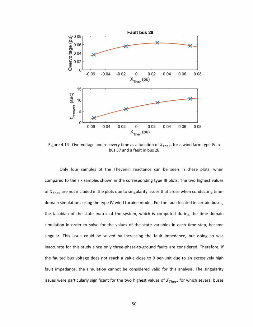
Figure 4.14 Overvoltage and recovery time as a function of 𝑋𝑇ℎ𝑒𝑣, for a wind farm

type IV in bus 37 and a fault in bus 28 ................................................................... 50

Figure 4.15 R-squared for the overvoltages as a function of 𝑋𝑇ℎ𝑒𝑣, for a wind farm

type IV .................................................................................................................... 51

Figure 4.16 R-squared for the recovery time as a function of 𝑋𝑇ℎ𝑒𝑣, for a wind farm

type IV .................................................................................................................... 52

Figure 4.17 Overvoltage and recovery time as a function of fault duration, for a wind

farm type III in bus 37 and a fault in bus 11 .......................................................... 54

Figure 4.18 Overvoltage and recovery time as a function of fault duration, for a wind

farm type III in bus 37 and a fault in bus 17 .......................................................... 54

Figure 4.19 Overvoltage and recovery time as a function of fault duration, for a wind

farm type III in bus 37 and a fault in bus 26 .......................................................... 55

xi

LIST OF EQUATIONS

Equation 1 Rotor direct current output of the type III wind turbine voltage controller ........ 13

Equation 2 Reactive power output of the type III wind turbine ............................................. 14

Equation 3 Direct current output of the type IV wind turbine voltage controller ................. 16

Equation 4 Reactive power output of the type IV wind turbine ............................................ 17

Equation 5 Series impedance of the π-nominal model of a transmission line ........................ 34

Equation 6 Shunt admittance of the π-nominal model of a transmission line ....................... 34

Equation 7 Per-length series impedance of the π-nominal model of a transmission line ...... 34

Equation 8 Per-length shunt admittance of the π-nominal model of a transmission line ...... 34

Equation 9 Series impedance of the π-equivalent model of a transmission line .................... 36

Equation 10 Shunt admittance of the π-equivalent model of a transmission line ................... 36

Equation 11 Propagation constant of a transmission line ........................................................ 36

Equation 12 Ohm’s law for voltage and current changes ......................................................... 39

Equation 13 Simplified Ohm’s law for voltage and current changes ........................................ 39

Equation 14 Superposition theorem for a power system ......................................................... 39

Equation 15 Superposition theorem for bus 𝑘 .......................................................................... 40

Equation 16 Thevenin impedance at bus 𝑘 ............................................................................... 40

Equation 17 Definition of 𝑅2 ..................................................................................................... 45

Equation 18 Definition of TSS .................................................................................................... 46

Equation 19 Definition of RSS .................................................................................................... 46

1

CHAPTER 1

INTRODUCTION

This Chapter serves as an introduction to the work developed in this thesis. The

motivation for conducting this research, along with its objective and the approach taken to

reach it are explained. The organization of the rest of the Chapters of the thesis is included at

the end of this Chapter.

1.1 Motivation and Background

First, the motivation for developing this work will be explained, summarizing the

enormous potential of wind energy but also the challenges that it poses to power systems.

These challenges are motivating major research in the area of wind power, given its many

advantages.

1.1.1 Wind Energy Opportunities and Challenges

Recently, there has been increasing interest in renewable energies due to public

awareness of the negative effects on the environment of conventional electricity generation

resources like coal and oil. The United States has enacted several renewable electricity

mandates, which are laws that require utilities to sell or produce a certain percentage of

electricity from renewable sources. Usually the required percentage of renewable electricity

increases over time until reaching a target percentage, such as 20 or 25 percent, at a target

year, such as 2020 or 2025. Twenty-nine states have renewable electricity mandates and an

additional six states have renewable electricity goals [1]. Due to some favorable characteristics

of wind over other renewables, wind generation has grown considerably in the last two decades

[2].

2

The New England region, which comprises of six states in the northeastern corner of the

US, possesses abundant potential for developing both inland and offshore wind power

generation. The New England Wind Integration Study showed that up to 12,000 MW could be

generated using this renewable source, as compared to the existing generating capacity of 800

MW [3], [4]. This same study pointed out that the region could generate up to 24% of its total

annual electric energy needs in 2020 using wind power, given that certain transmission

upgrades are performed. Most of New England’s wind resources are located in the state of

Maine, where Maine’s Renewable Electricity Mandate set a goal for 8,000 MW of installed wind

capacity by 2030, which implies a significant rise compared to the 600 MW of current wind

generation [5].

It is important to point out that inland wind resources are primarily in remote locations

far from major load centers, particularly in the Northern New England region, as shown in Figure

1.1. Therefore, long transmission lines are required to connect the wind farm to the rest of the

power grid, placing them in a weak point of the system. As opposed to other generation

resources like nuclear or gas, whose location can be chosen by the system planners, the location

of a wind farm is selected primarily based on good wind conditions, although it is also subject to

environmental and economic constraints [6], [7].

3

Figure 1.1 Wind resources and load centers in the New England Region [3]

As summarized in the previous paragraphs, wind generation has great potential,

particularly in the New England region. However, integrating wind generation into the existing

grid poses some significant challenges from the electrical point of view, particularly due to the

limited reactive power capability that wind turbines have. This can cause several voltage

problems, such as important voltage drops or rises and fluctuation at the point of connection

with the rest of the power grid [8], [9]. Although modern wind generators include power

electronics converters which have some reactive power regulation capability that allows certain

control over voltage disturbances, the capacity of the power electronics is limited [10]. When a

contingency occurs in the system, the inability of wind turbines to provide enough reactive

4

power so that the voltage can go back to its pre-fault value is a major concern. Therefore,

dynamic voltage stability, which is defined as the ability of a power system to maintain steady

voltages at all buses after a disturbance, is one of the biggest issues regarding wind integration.

It should also be pointed out that it is essential to take into account the distinctive features of

wind power, such as its usually remote geographical location, when conducting wind integration

studies.

Typical wind generation project proposals assume a basic configuration, which just

include wind turbines as part of the wind farm. The System Impact Studies (SIS) often identify

additional system elements needed to assure that the proposed generation does not degrade

the power system performance. These additional system condition installations appear often as

significant economic burdens. The present study focuses on analyzing basic wind installations in

order to identify the appropriate actions that should be taken to improve their dynamic voltage

performance.

1.1.2 Analysis of Existing Literature

As mentioned in Section 1.1.1, dynamic stability is one of the biggest concerns when

conducting wind integration studies. Several studies have analyzed it, such as [11], [12], [13] and

[14]. However, they are not always focused on dynamic voltage performance, but also on other

dynamic magnitudes such as rotor angles. This comes in detriment of a more insightful study of

dynamic voltage issues. Some studies like [15] have focused on developing single and

aggregated wind turbine models for dynamic simulations, a necessary tool for any wind

integration study like the present thesis. Probably the most comprehensive study on dynamic

behavior of both inland and offshore wind farms to date is [16]. Mechanical characteristics of

wind turbines are taken as a starting point to explain their electrical behavior. However, its focus

5

is not only on voltage performance, but also on several other dynamic magnitudes such as rotor

speed. Furthermore, it does not study the effect of the transmission line connecting wind farms

to the rest of the system.

Therefore, there is still a need for studies focusing on dynamic voltage behavior of

inland wind farms, which are still by far the mainstream in wind power, while taking into

consideration the long transmission lines that typically connect them to the rest of the power

grid.

For the present thesis, two kinds of wind turbines have been considered: wind turbines

type III and type IV, as they are the dominant types in the market. Type III wind turbines are the

most widely used nowadays, and several studies such as [11], [12], [13], [14] have analyzed their

dynamic voltage performance using different approaches. However, type IV wind turbines are

expected to increase their market share due to their several advantages and sustained cost

reduction, and might eventually become the leading type of wind turbine. In spite of these

advantages, few studies have been conducted about this turbine technology and its effects on

the grid are not widely known [17]. Reference [18] compared the performance of both these

kinds of turbines, focusing on rotor speed issues. Literature is scarce regarding dynamic voltage

stability studies considering wind IV turbines, as available studies focus on developing control

strategies as in [19], [20], [21]. The present thesis will analyze both wind turbine types, with the

aim of shedding some light on the impact of type IV wind turbines.

As mentioned in Section 1.1.1, most wind farms are in remote locations and connected

through long transmission lines to the rest of the network, which places them in a weak point of

the system. Therefore, it is important to analyze the impact that the interconnection between

the wind farm and the rest of the grid has on the system’s dynamic performance, and some

6

studies have dealt with this issue. References [22], [22], [23], [24], [24] consider this matter and

analyze, among many other issues such as power-swing stability, the implications of several

control schemes for improving wind farm’s voltage performance when connected to the grid

through a weak link. Other studies such as [25] share the practical experience of transmission

planners dealing with the issue of connecting wind farms to a real power system.

Instead of studying the impact of wind turbines, so that the appropriate actions to

remediate the problems can be identified, these studies focus on developing control methods to

improve its performance. However, there might be alternative solutions to the problem of poor

dynamic voltage performance of basic wind installations, which may be simpler and/or most

cost-effective. In addition, most of this research work only considers induction-generator-based

wind turbines, leaving out type IV wind turbines.

Many of these studies use the Short Circuit Ratio, a magnitude related to the Thevenin

impedance equivalent of the grid, as a measure of the strength of the interconnection. The use

of the Thevenin impedance as such to characterize the severity of a fault from a dynamic voltage

point of view, which is presented in Chapter 4 of this thesis, is novel. The concept of Thevenin

impedance has been used in wind studies to conduct short-circuit analysis in works such as [26],

[27], but not in dynamic voltage studies.

As a conclusion for this literature review, it should be pointed out that there is a need

for research focusing on dynamic voltage behavior of inland wind farms, while taking into

consideration the long transmission lines that connect them to the rest of the power grid.

Furthermore, type IV wind turbines need to be further studied, given their projected increase in

market share and the very scarce literature currently available.

7

1.2 Research Objective

The aim of the present thesis is to analyze voltage characteristics of an electric grid

connected to wind generation and subject to fault conditions. Given the continuous increase of

wind power in the world, the need for studies such as this one becomes critical in order to

maintain power quality and stability.

Both type III and type IV wind turbines are to be studied, with the goal of expanding the

current knowledge of type III performance and throwing some light on the impact of type IV

wind turbines. The ultimate objective of conducting such a study is to be able to identify

appropriate actions than can remediate the voltage problems caused by wind generation.

While this is an academic study, its practical application has always been on the

spotlight of the researchers. The typically remote location of wind resources, particularly in the

New England region, makes it necessary to use long transmissions lines to connect wind farms

to the rest of the power system. That is why studying the effects of such an electrical connection

on voltage performance is one of the cornerstones of this work.

1.3 Research Approach

In order to achieve the goal of quantifying the impact of wind power on dynamic voltage

performance of a power grid, several simulations have been conducted. The IEEE standard 39-

bus system, which is a simplified representation of the New England electric grid, has been used

as a platform to show the result of the study. The software used to conduct the simulations is

the Power System Analysis Toolbox (PSAT) for MATLAB, a research-oriented software which

gives the user great flexibility and the ability of easy prototyping when compared to commercial

tools.

8

First of all, the performance of synchronous machines and wind turbines type III and IV

has been compared. Simulations have been conducted considering synchronous machines and

wind turbines subject to the same faults, in order to quantify how the inclusion of a certain kind

of wind turbine affects dynamic voltage profiles. In addition, several wind penetration scenarios

have been analyzed, which show the impact of a higher wind generation share.

In order to study the impact of a long transmission line connecting the wind farm to the

system, several cases of increasing line length have been considered. These cases have been

simulated under different fault conditions in the system. The Thevenin impedance seen by the

wind bus has been used as a measure of the strength of the point of interconnection, and its

relation with several variables that characterize the effects of a fault has been determined.

1.4 Thesis Organization

The organization of the remaining Chapters of this thesis can be summarized as follows:

Chapter 2 discusses the models of the different power system’s elements and devices

used in this study, such as synchronous generators, wind turbines and transmission lines. An

explanation of the automated simulation process and analysis of results that has been

developed for this thesis is also included in this Chapter.

Chapter 3 deals with the different performance of wind turbines and synchronous

generators regarding system voltages. Several wind integration scenarios are considered in

order to quantify the impact of increasing wind power in the network.

In Chapter 4, the impact that the interconnection of a wind farm has on the system’s

dynamic voltage performance is analyzed. The Thevenin impedance seen by the wind bus has

been used as a measure of the strength of the point of interconnection, and its relation with

several variables that characterize the effects of a fault has been determined.

9

This thesis concludes with Chapter 5, which includes the conclusions extracted from the

thesis’s results and the related topics that should be further investigated in future research

studies.

10

CHAPTER 2

POWER SYSTEM MODELING AND SIMULATION

This Chapter discusses the models of the different power system’s elements and devices

used in this study, such as synchronous generators, wind turbines and transmission lines. An

explanation of the automated simulation process and analysis of results that has been

developed for this thesis is also included at the end of this Chapter.

2.1 Simulation Tool: Power System Analysis Toolbox

The software used to conduct the simulations is the Power System Analysis Toolbox

(PSAT) for MATLAB. PSAT is an open-source, freeware, power system analysis toolbox that can

be used for power system analysis and control learning, education and research. It is a research-

oriented software which gives the user more flexibility and the ability of easy prototyping when

compared to commercial tools, which are focused on achieving computational efficiency.

In addition, PSAT has been used for several wind integration studies such as [28], [29],

[30], [31]. One of the reasons for its use in wind power analysis is the wind turbine models that

PSAT includes, which are based on the models developed in [32], particularly created for

conducting dynamic analysis. Furthermore, the wind turbine models implemented in PSAT are

adequate for representing a single machine as well as a wind park composed of several

generators.

On the other hand, PSAT has some limitations. As mentioned before, it strengthens

flexibility for the user in detriment of computational efficiency, which makes it unsuitable for

studying real power systems containing thousands of buses. However, this thesis is an academic

work which uses IEEE 39-bus system instead of a real power grid as the platform to conduct the

11

study. The 39-bus test case has been chosen due to its numerous advantages when used for

research work, which will be discussed in Section 2.2. Therefore, PSAT is a perfectly valid

simulation package for the present work.

As most power system simulation packages, PSAT uses the single phase equivalent

representation of a power system. This is an acceptable representation when three-phase

balanced magnitudes are considered all over the power system, as it is assumed in this thesis.

In the following Sections, the models of the devices of interest for the present study are

going to be discussed. For a detailed description of the rest of the models of power system’s

elements included in PSAT, please refer to [32]. A brief description of the physical fundamentals

of each of the devices is also included in the following Sections.

2.1.1 Synchronous Generator Model

Large-scale power is mainly generated by three-phase synchronous generators, which

are the traditional type of generators, driven by steam, hydro or gas turbines in all the

conventional power generation facilities before the rise of renewables. The synchronous

generator has two main components: the stator and the rotor. The stator contains the armature

windings, which are designed to generate balanced three-phase voltages. The rotor contains the

field windings, and its function is to induce voltages in the stator’s winding by means of a

rotating magnetic field. In order for this magnetic field to be created, a DC excitation system is

used to inject a direct current into the rotor’s windings. Moreover, the rotor constantly rotates

because it is connected to the already mentioned steam, hydro or gas turbine, and this rotation

makes the magnetic field change over time [33].

12

The synchronous machine model used in PSAT simulations in this thesis represents an

order II synchronous machine, which corresponds to the classic electro-mechanical model, used

for deducing the classical swing equations in the literature [34]. This model considers a constant

amplitude excitation voltage of the rotor windings.

Figure 2.1 Schematic of a three-phase synchronous generator [35]

2.1.2 Wind Turbine Type III Model

The dominant type of wind turbine in the world is the doubly-fed induction generator

(DFIG), also known as type III wind turbine [36]. The electric generator it contains is composed

by a rotor and a stator, just like the synchronous machine. The stator is directly connected to

the grid via a transformer, while the rotor windings are also connected to the grid via slip rings,

an AC to AC power electronic converter and a transformer. The power electronic converter

allows the DFIG to supply energy to the grid at the required 60 Hz frequency, regardless of the

rotor speed, which is determined by the speed of the wind. With this configuration the energy is

delivered to the grid from both the stator and the rotor, hence the term “doubly-fed” [37].

13

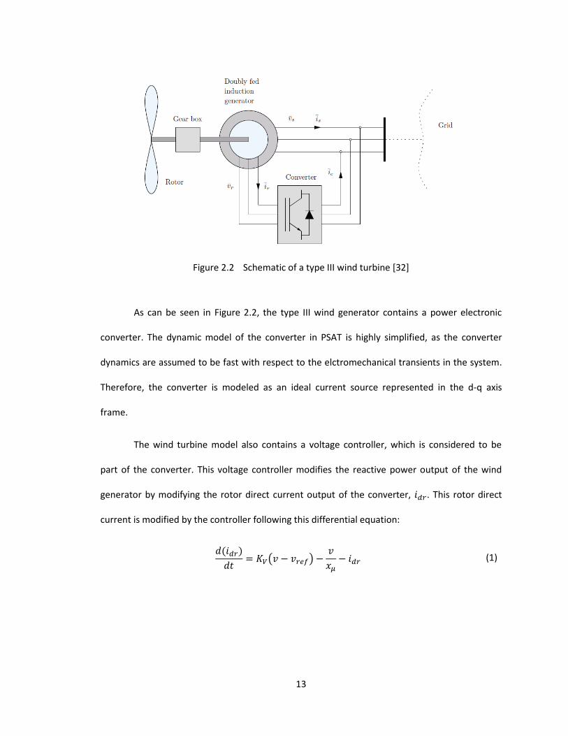
Figure 2.2 Schematic of a type III wind turbine [32]

As can be seen in Figure 2.2, the type III wind generator contains a power electronic

converter. The dynamic model of the converter in PSAT is highly simplified, as the converter

dynamics are assumed to be fast with respect to the elctromechanical transients in the system.

Therefore, the converter is modeled as an ideal current source represented in the d-q axis

frame.

The wind turbine model also contains a voltage controller, which is considered to be

part of the converter. This voltage controller modifies the reactive power output of the wind

generator by modifying the rotor direct current output of the converter, 𝑖𝑑𝑟. This rotor direct

current is modified by the controller following this differential equation:

𝑑(𝑖𝑑𝑟)

𝑑𝑡= 𝐾𝑉(𝑣 − 𝑣𝑟𝑒𝑓) −

𝑣

𝑥𝜇− 𝑖𝑑𝑟 (1)

14

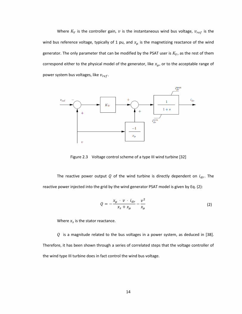
Where 𝐾𝑉 is the controller gain, 𝑣 is the instantaneous wind bus voltage, 𝑣𝑟𝑒𝑓 is the

wind bus reference voltage, typically of 1 pu, and 𝑥𝜇 is the magnetizing reactance of the wind

generator. The only parameter that can be modified by the PSAT user is 𝐾𝑉, as the rest of them

correspond either to the physical model of the generator, like 𝑥𝜇, or to the acceptable range of

power system bus voltages, like 𝑣𝑟𝑒𝑓.

Figure 2.3 Voltage control scheme of a type III wind turbine [32]

The reactive power output 𝑄 of the wind turbine is directly dependent on 𝑖𝑑𝑟. The

reactive power injected into the grid by the wind generator PSAT model is given by Eq. (2):

𝑄 = −𝑥𝜇 · 𝑣 · 𝑖𝑑𝑟

𝑥𝑠 + 𝑥𝜇−

𝑣2

𝑥𝜇 (2)

Where 𝑥𝑠 is the stator reactance.

𝑄 is a magnitude related to the bus voltages in a power system, as deduced in [38].

Therefore, it has been shown through a series of correlated steps that the voltage controller of

the wind type III turbine does in fact control the wind bus voltage.

15

2.1.3 Wind Turbine Type IV Model

The second-most used type of wind turbine in the world is the direct-drive synchronous

generator wind turbine (DDSG), also known as type IV. Type IV wind turbine is expected to

increase its market share due to its several advantages such as its improved efficiency,

suppression of noise, and lower maintenance cost than DFIG [17].

The type IV wind turbine has basically the same structure as the synchronous machine.

However, there is one fundamental difference: the rotor of a synchronous generator can rotate

at a chosen speed, as its rotational speed is controlled by the input of the steam, hydro or gas

turbine connected to it. On the other hand, due to the stochastic nature of wind, the rotor of a

type IV wind turbine cannot rotate at a fixed speed without a significant loss of efficiency.

Therefore, the AC energy generated by the type IV wind turbine, whose frequency changes with

the variability of wind, must be converted into 60 Hz AC energy suitable for being transmitted in

a North American power system. Then, the AC output of the wind generator is first rectified into

DC and then inverted back to AC at standard 60 Hz grid frequency. The AC-AC conversion is

achieved by means of a power electronics device, which decouples the wind turbine from the

grid [37].

Figure 2.4 Schematic of a type IV wind turbine [32]

16

As can be seen in Figure 2.4, the wind generator type IV also contains a power electronic

converter. The converter dynamics are assumed to be fast with respect to the elctromechanical

transients in the system, as they are for the wind generator type III, which highly simplifies the

type IV converter model in PSAT. Therefore, the converter is modeled as an ideal current source

represented in the d-q axis frame.

The wind turbine model also contains a voltage controller, which is considered to be

part of the converter. This voltage controller modifies the reactive power output of the wind

generator by modifying the converter direct current output, 𝑖𝑑𝑐. This direct current output is

modified by the controller following this differential equation:

𝑑(𝑖𝑑𝑐)

𝑑𝑡=

𝐾𝑉(𝑣𝑟𝑒𝑓 − 𝑣) − 𝑖𝑑𝑐

𝑇𝑉 (3)

Where 𝐾𝑉 is the controller gain, 𝑣𝑟𝑒𝑓 is the reference bus voltage, 𝑣 is the instantaneous

wind bus voltage and 𝑇𝑉 is the voltage controller time constant. The parameters that can be

modified by the PSAT user are 𝐾𝑉 and 𝑇𝑉.

Figure 2.5 Voltage control scheme of a type IV wind turbine [32]

17

The reactive power output 𝑄 of the wind turbine is directly dependent on 𝑖𝑑𝑐. The PSAT

wind turbine type IV model includes, as most turbines of this kind, a permanent magnet rotor

(PMG), which means that the power factor of the generator is equal to 1. Therefore, the

reactive power output of the stator is 0, and all the reactive power injected to the grid is

controlled by the power electronics converter. Then, the 𝑄 output of the generator becomes:

𝑄 = 𝑖𝑑𝑐

𝑣

cos 𝜃+ 𝑃 tan𝜃 (4)

Where 𝜃 is the phase angle of the wind bus voltage and 𝑃 is the active power output of

the type IV wind generator.

As mention in Section 2.1.3, 𝑄 is a magnitude related to the bus voltages in a power

system. Therefore, it has been shown through a series of correlated steps that the voltage

controller of the type IV wind turbine does in fact control the wind bus voltage.

2.1.4 Transmission Line Model

It is convenient to represent a balanced three-phase transmission line by the two-port

network shown in Figure 2.6, where 𝑉𝑆 and 𝐼𝑆 Is are the sending-end voltage and current and 𝑉𝑅

and 𝐼𝑅 are the receiving-end voltage and current [39]. This lumped equivalent model of a

transmission line, also called the π-nominal circuit due to its shape similarity with the Greek

letter, is an acceptable representation for most studies, and it is the model implemented in

PSAT. The magnitudes 𝑍 and 𝑌 are usually calculated by multiplying the line per-length

impedance 𝑧 and per-length admittance 𝑦 by the total line length, respectively. A correction

factor should be applied to 𝑍 and 𝑌 when considering long transmission lines, a matter that is

discussed in Section 4.1.

18

Figure 2.6 π-nominal model of a transmission line

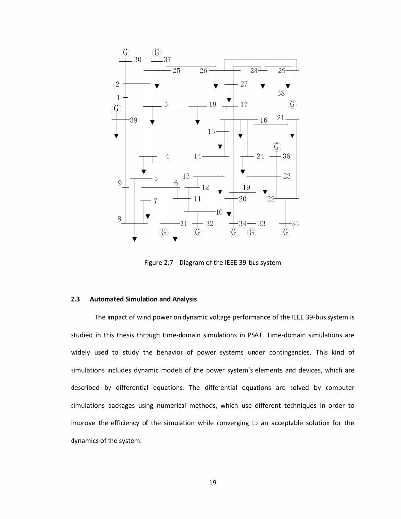
2.2 IEEE 39-Bus Test Case

The platform used to conduct this study is the IEEE standard 39-bus system, which

represents a greatly reduced model of the New England electric grid. The 39-bus system is a

standard system for testing new methods, which has been used by numerous researchers to

study both static and dynamic problems in power systems. Using test systems is considered

more convenient than using models of real power systems, as the latter are not fully

documented and tend to be very big, which makes it difficult to distinguish general trends.

Furthermore, the results obtained with models of real systems are less generic than those

obtained with test systems [15].

The IEEE 39-bus system has 10 generators, 19 loads, 36 transmission lines and 12

transformers, as can be seen in Figure 2.7.

19

Figure 2.7 Diagram of the IEEE 39-bus system

2.3 Automated Simulation and Analysis

The impact of wind power on dynamic voltage performance of the IEEE 39-bus system is

studied in this thesis through time-domain simulations in PSAT. Time-domain simulations are

widely used to study the behavior of power systems under contingencies. This kind of

simulations includes dynamic models of the power system’s elements and devices, which are

described by differential equations. The differential equations are solved by computer

simulations packages using numerical methods, which use different techniques in order to

improve the efficiency of the simulation while converging to an acceptable solution for the

dynamics of the system.

G G

GG

G

GG GG G

30

39

1

2

25

37

29

17

26

9

3

38

16

5

4

18

27

28

3624

35

22

21

20

34

23

19

33

10

11

13

14

15

831

126

32

7

20

Throughout the work leading to the completion of this thesis, several MATLAB scripts

have been developed in order to automatize both the time-domain simulations and the analysis

of their results. These scripts perform several tasks which include placing three-phase to ground

faults in all buses of the system and running time-domain simulations for each case, while

recording some magnitudes of interest to this study such as dynamic bus voltages.

Once these magnitudes are recorded, the developed MATLAB scripts also perform an

analysis of the simulation results, saving the PSAT user time from tedious manual calculations.

The developed code calculates voltage peaks and sags and recovery times, as shown in Figure

2.8, and runs a statistical analysis of the overall results. In this particular example shown in

Figure 2.8 a voltage overshoot can be observed, but the scripts also consider cases in which

there are voltage oscillations until returning back to pre-fault values, and properly calculate the

recovery time in each case.

21

Figure 2.8 Graphical explanation of voltage overshoot and time recovery calculations

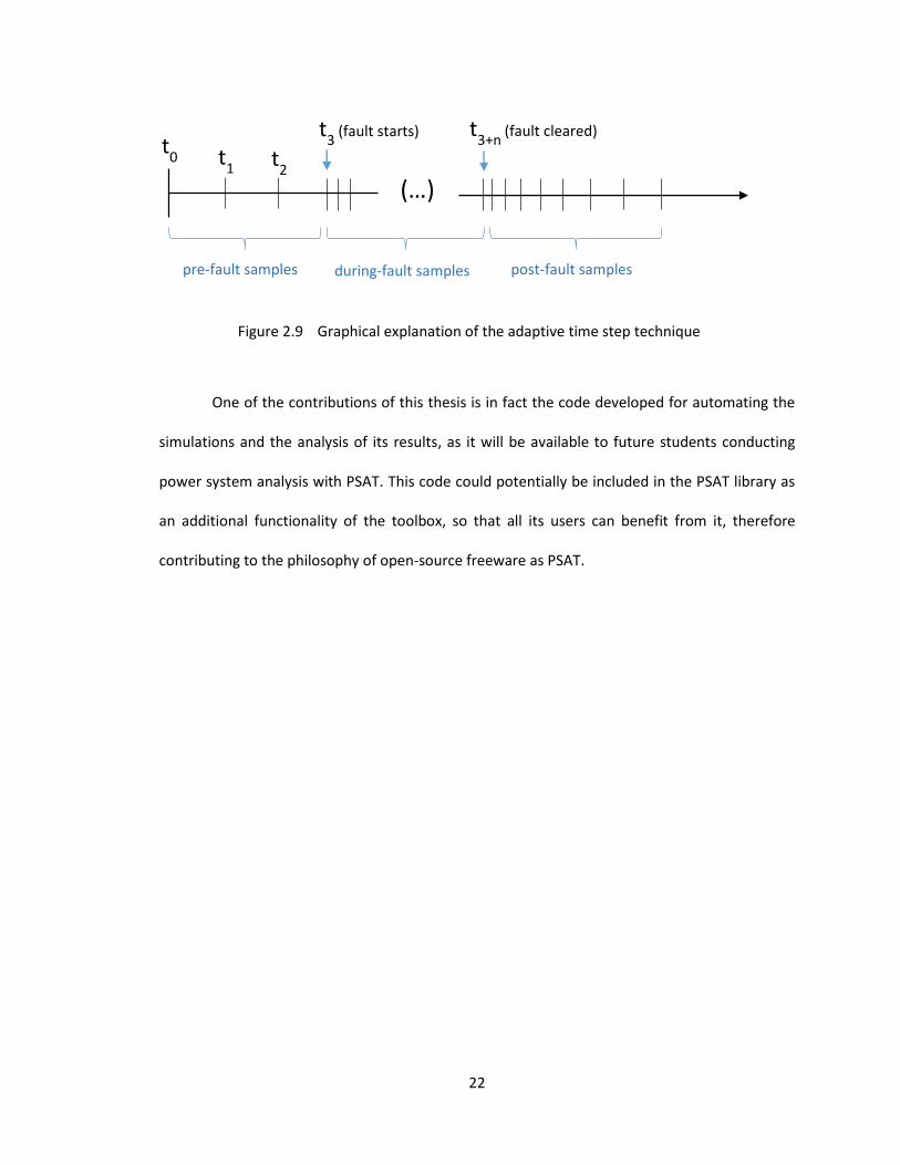
One of the techniques used in this thesis to improve the time efficiency of time-domain

simulations in PSAT is the adaptive time step. This technique, which is utilized in other

disciplines such as Neural Network training algorithms, makes use of a longer time step when

the change in the magnitude of system variables is small, but reduces the time step when an

event happens in the system, in order to increase the accuracy of the simulation. In the time-

domain simulations conducted in PSAT, big time steps are used in the pre-fault and far post-fault

time frame, while small time steps are used while the fault is happening or it has been recently

cleared. A graphical explanation of the adaptive time step can be found in Figure 2.9, where an

n-samples-long fault is considered. The code developed in the present thesis to automatize the

analysis of the time-domain simulations takes into account the fact that a dynamic sampling rate

is used throughout the simulation, which is adjusted by the adaptive time step algorithm.

Voltage overshoot

trecovery

22

Figure 2.9 Graphical explanation of the adaptive time step technique

One of the contributions of this thesis is in fact the code developed for automating the

simulations and the analysis of its results, as it will be available to future students conducting

power system analysis with PSAT. This code could potentially be included in the PSAT library as

an additional functionality of the toolbox, so that all its users can benefit from it, therefore

contributing to the philosophy of open-source freeware as PSAT.

t0 t

1 t

2

t3

(fault starts)

(…)

t3+n

(fault cleared)

pre-fault samples during-fault samples post-fault samples

23

CHAPTER 3

COMPARISON OF WIND TURBINES AND SYNCHRONOUS GENERATORS’ PERFORMANCE

A comparison of the dynamic voltage performance of synchronous machines and basic

wind installations under fault conditions in the system is presented in this Chapter. Both wind

turbines type III and type IV are to be studied, with the goal of expanding the current knowledge

of type III performance and shedding some light on the impact of type IV wind turbines. In

addition, several wind integration scenarios are considered in order to quantify the impact of

increasing wind power in the network.

3.1 Low-Wind-Penetration Scenario

In the first place, a general analysis of the voltage performance of wind farms under

contingencies in the system will be presented. This performance has been compared with that

of synchronous machines subject to the same faults. The same simulations have been

conducted using both synchronous machines and wind farms, in order to quantify how the

inclusion of wind generation affects dynamic voltage profiles.

The IEEE 39-bus test case power system was used as the case study to show the

developed methodology. The original 39-bus system, from now on referred to as the original

case, contains ten synchronous machines as sources of electric power. The effects of wind

penetration in this system have been studied by connecting some wind farms to it, while the

total amount of generation in the system has been kept constant. Thus, when including a certain

amount of wind generation, the amount of power generated by synchronous machines has been

reduced accordingly.

24

For this study, two kinds of wind farms have been considered: type III and type IV, due

to several factors discussed in previous Chapters. The PSAT wind turbine models used for the

simulations, which are discussed in Chapter 2, are adequate for representing a wind farm

composed of several generators, and they were used as such in all the simulations in this thesis.

This aggregate model of a wind generator includes the differential equations corresponding to

the dynamic model of just one turbine, because modelling each of the hundreds of turbines that

constitute a wind far would make the simulations tremendously inefficient. However, the model

makes certain calculations in order to take into account the contribution of all the wind turbines

in the farm while maintaining the efficiency of the simulations, as discussed in [15].

Every wind farm used was composed of 500 units with a power rating of 2 MVA each, in

order to make them equivalent to each of the synchronous generators in the original case. The

inertia of the wind farm was set to be equal to the inertia of the synchronous machines, as well

as its voltage level. It is important to point out that synchronous generators typically have a

higher inertia than wind turbines. However, this study focuses on the inherent voltage

characteristics of wind turbines and synchronous generators so, in order to compare them in a

one-to-one basis, the inertia, which is related to phase-angle stability rather than voltage

stability, was set equal. The rest of the parameters of the wind farm were set to its default

values in PSAT. The wind speed profile was assumed to be constant over time in all simulations,

which is a realistic assumption given that the time interval considered in all simulations is just a

few seconds long.

The voltage controllers of the wind turbines will play a significant role in the dynamic

voltage performance of the system. The parameters of the voltage controllers of both wind type

III and type IV wind turbines were set to equal values, in order to compare both types of

turbines on a one-to-one basis. The voltage control gain of both types of turbines, 𝐾𝑉, was set to

25

the default value of 10, while the time constant of the type IV controller, 𝑇𝑉, was set to 1 second

in order to make it equivalent to the type III controller, which has a fixed time constant of 1

second. More details about the voltage controllers of both wind turbine models can be found in

Sections 2.1.2 and 2.1.3.

Instead of studying the different voltage performance when modifying the controller

parameters, this study focuses analyzing the impact of wind turbines, so that the appropriate

actions to remediate the problems can be identified. Much of the literature analyzed in Section

1.1.2 deals with developing several control schemes to improve wind turbines’ performance.

However, there might be alternative solutions that may have advantages over this strategy. In

addition, the vast majority of the solutions offered by these studies propose the refinement of

the turbine voltage controller gains on a case-to-case basis, which have therefore limited

positive effect as they are not universal, as pointed out by [24].

3.1.1 Measurement of the Strength of the System

In this Section, the strength of the system in a low-wind-penetration scenario is going to

be measured. The strength is defined in this case as how severe of a contingency the system can

withstand in terms of fault duration, regardless of the fault location. The system withstands a

fault when all the bus voltages are able to return to its pre-fault value.

Using the original case, which includes ten synchronous machines, a three-phase-to-

ground fault was simulated in every bus of the system, one bus at a time. The duration of the

fault was increased in 0.1-second intervals until any bus in the system became unstable due to

an angular loss of synchronism of the system’s generators. This occurred for a 0.4-second-long

fault, for which three fault locations made the system unstable. These fault locations that lead

the system to instability were bus 29, a load bus, and buses 37 and 38, generator buses.

26

The same simulations were conducted again, but considering two low-wind-penetration

scenarios instead of the original case. These two scenarios were created by replacing the

synchronous generator in bus 37 by a wind farm of type III and type IV, which correspond to a

10% of wind penetration. As mentioned before, the inertia, voltage level and generating

capacity of the wind farms were equal to those of the synchronous generator they replaced.

Again, 0.4-second-long, three-phase-to-ground faults were applied to every bus in the

system. It is important to point out that no lines were opened so that the post-fault system

topology remained unchanged. The simulation results in both cases were the same as in the

synchronous machine case: faults located in buses 29, 37 and 38 lead the system to instability.

This concludes that the 10% wind penetration scenario does not deteriorate the system’s post-

fault, steady-state voltage stability.

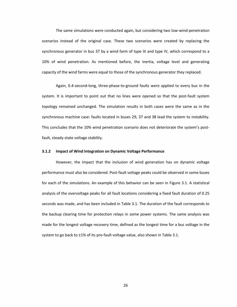
3.1.2 Impact of Wind Integration on Dynamic Voltage Performance

However, the impact that the inclusion of wind generation has on dynamic voltage

performance must also be considered. Post-fault voltage peaks could be observed in some buses

for each of the simulations. An example of this behavior can be seen in Figure 3.1. A statistical

analysis of the overvoltage peaks for all fault locations considering a fixed fault duration of 0.25

seconds was made, and has been included in Table 3.1. The duration of the fault corresponds to

the backup clearing time for protection relays in some power systems. The same analysis was

made for the longest voltage recovery time, defined as the longest time for a bus voltage in the

system to go back to ±1% of its pre-fault voltage value, also shown in Table 3.1.

27

Figure 3.1 Voltage profiles of four of the system buses for a fault located in bus 4

Table 3.1 Statistical analysis of the dynamic voltage performance of synchronous and wind

generators

Overvoltage peak Recovery time

Synchronous machine

Mean: 1.067 pu Mean: 1.20 sec

Std deviation: 0.004 pu Std deviation: 0.63 sec

Wind type III Mean: 1.071 pu Mean: 1.38 sec

Std deviation: 0.008 pu Std deviation: 0.55 sec

Wind type IV Mean: 1.116 pu Mean: 3.79 sec

Std deviation: 0.030 pu Std deviation: 1.90 sec

Wind farm bus

28

Section 3.1.1 shows that the steady-state voltage stability of the system is not

deteriorated due to the addition of wind, so one can conclude that the dynamic performance

deterioration in this low-wind-penetration case is due to the wind controllers’ action, and not to

a lack of reactive power capability of the wind turbines. Therefore, tuning the wind voltage

controller parameters seems to be the most sensible approach in this case, in order to improve

the dynamic voltage performance of the system.

It is also important to realize that the type IV wind turbines show a worse dynamic

performance than type III. Type IV wind turbines are thought to behave better in terms of

voltage stability than wind type III, due to the bigger power electronics converter they possess,

which provides them with higher reactive power capability. However, the lack of reactive power

is not an issue for either of the wind turbine types in this case, as show the results in Section

3.1.1. Therefore, the different voltage control scheme of the PSAT type III and type IV models

should be further investigated, as it is the cause of the worse performance shown by type IV.

Although the control parameters of both turbine types were set to the same values, the voltage

control schemes of type III and IV are partially different, as discussed in Sections 2.1.2 and 2.1.3.

It should also be studied to what extent this control schemes can be modified, as they

do not only depend on the structure of the voltage controller, but also on the 𝑄 output of the

machines. That is because the 𝑄 output of type III and IV wind turbines, described by Eq. (2) and

Eq. (4), respectively, is partially determined by the inherent physical characteristics of each type

of turbine.

As can be seen in Figure 3.2, tuning the controller gain does in fact change the voltage

response of the wind bus. The left-hand plot represents the voltage performance of the wind

bus when using the default gain of the wind turbine voltage controller, while the right-hand plot

29

shows the behavior of an adjusted gain for that particular fault. However, the present thesis did

not focus on adjusting the controller gains because, as pointed out by [24], these adjustments

are performed on a case-to-case basis. In addition, wind turbines developed by different

manufacturers might have different controller schemes, so a study dealing with modifying

generic controller gains would have rather limited practical usefulness. The real wind turbine

models developed by different manufacturers are proprietary, and are usually provided to

power system planners as a “black box” model. However, many efforts have been put to

develop generic models as the ones used in PSAT [15]. While the dynamic model of different

brand wind turbines can be well represented by a generic model, as all of them are based on the

same working principles, the tuning of a generic controller model cannot be exported to a

different controller, as it is highly dependent on the particular controller scheme.

Figure 3.2 Effect of tuning the wind turbine controller on voltage performance

30

3.2 Increasing Wind Penetration

Once the dynamic voltage deterioration due to a 10% wind penetration was shown, as

presented in Section 3.1.2, several cases of wind penetration were considered. The objective

was to compare the effects that a three-phase fault has on an increasing wind penetration

scenario. Seven cases were considered: the original 39-bus system including its ten synchronous

machines; 10% penetration of wind type III; 20% penetration of wind type III; 30% penetration

of wind type III; 40% penetration of wind type III; 10% penetration of wind type IV; and 20%

penetration of wind type IV. The wind farms were progressively added to buses 37, 30, 38 and

39 to reach the 40% penetration scenario. For this study, a three-phase-to-ground, 0.25-second-

long fault located in bus 17 was considered. As a starting point for this wind integration study,

bus 17 was chosen due to its middle distance from the wind farm buses in the 39-bus test case.

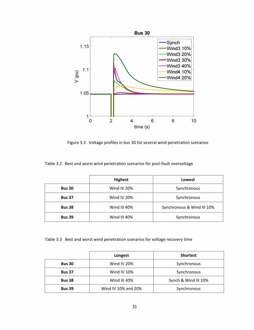
The results of these simulations have been summarized in Table 3.2 and Table 3.3. For

each of the seven cases, the best and worst voltage performance was recorded. An example of

the transient voltage profiles in bus 30 obtained for the different cases can be seen in Figure 3.3.

31

Figure 3.3 Voltage profiles in bus 30 for several wind penetration scenarios

Table 3.2 Best and worst wind penetration scenarios for post-fault overvoltage

Highest Lowest

Bus 30 Wind IV 20% Synchronous

Bus 37 Wind IV 20% Synchronous

Bus 38 Wind III 40% Synchronous & Wind III 10%

Bus 39 Wind III 40% Synchronous

Table 3.3 Best and worst wind penetration scenarios for voltage recovery time

Longest Shortest

Bus 30 Wind IV 20% Synchronous

Bus 37 Wind IV 10% Synchronous

Bus 38 Wind III 40% Synch & Wind III 10%

Bus 39 Wind IV 10% and 20% Synchronous

32

The synchronous generator always shows the best performance, although the type III

10% penetration scenario had very similar voltage profiles in most of the cases. However, the

progressive addition of wind deteriorates the dynamic response of the voltages. This result

agrees with previous studies which state that for high penetration levels of wind energy in the

grid, the impacts to the system become of great concern [6], [8], [9]. In addition, it can be seen

that type IV shows a worse performance than type III, even for lower penetration scenarios. This

result confirms the conclusions from Section 3.1.2, pointing towards the different voltage

control schemes of the type III and type IV turbines as the cause for the worse dynamic

performance shown by type IV.

33

CHAPTER 4

INFLUENCE OF WIND FARM POINT OF INTERCONNECTION

The influence that the point of electrical interconnection between a wind farm and the

rest of the power system has on the bus voltages’ performance has been analyzed in this

Chapter. As most wind farms are in remote locations where the wind conditions are optimum

for obtaining electric energy, they are usually connected through long transmission lines to the

rest of the network, which places them in a weak point of the system. That is why studying the

effects of such an electrical connection on voltage performance is one of the cornerstones of

this work.

In the present study, several interconnection scenarios have been analyzed by using the

Thevenin impedance seen by the wind bus, which was used as a measure of the strength of the

interconnection. These different interconnection scenarios were created by adding a

transmission line between the wind farm’s step-up transformer and the rest of the network, and

modifying its model parameters appropriately. The relation between the Thevenin impedance

and two variables that characterize the effects of the fault, such as the time interval until the

voltage returns to normal conditions and the highest difference between the pre-fault and post-

fault voltages is presented.

It is important to point out that previous studies dealing with the issue of weak

connections of wind farms used the Short Circuit Ratio as a measure of the strength of the

connection. The use of the Thevenin impedance for analyzing the impact of the transmission line

on dynamic voltage performance is novel.

34

For this study, a 10% wind penetration scenario was considered, using both wind

turbines type III and type IV. One of the ten synchronous machines in the original 39-bus test

case was substituted by a wind farm of the same MVA rating, voltage rating and inertia. This

procedure is equivalent to the one used in Section 3.1.1.

4.1 Description of Line Length Increase

The π-nominal model of a transmission line discussed in Section 2.1.4 is used

throughout this thesis to represent a transmission line, as in most power system studies. The

series impedance 𝑍 and shunt admittance 𝑌 in Figure 2.6 can be calculated using Eq. (5) and Eq.

(6):

𝑍 = 𝑧 𝑙 (5)

𝑌 = 𝑦 𝑙 (6)

Where 𝑙 is the line length and 𝑧 and 𝑦 are the per-length impedance and admittance of

the line, given by Eq. (7) and Eq. (8):

𝑧 = 𝑅 + 𝑗𝜔𝐿 (7)

𝑦 = 𝐺 + 𝑗𝜔𝐶 (8)

Where 𝑅, 𝐿, 𝐺, 𝐶 are the per-length resistance, inductance, conductance and

capacitance of the line, respectively. The imaginary unit is symbolized as 𝑗, while 𝜔 stands for

the frequency of the AC energy flowing through the lines, which is of 2π60 rad/s in a North

American power system. 𝐺 is usually neglected in 60-Hz lines, so it is not included in the π-

representation of the line. These per-length parameters 𝑅, 𝐿 and 𝐶 depend on the physical

characteristics of the line, such as the type of conductor used, the number of wires per electrical

35

phase, the spacing between the phases and the addition or omission of a neutral conductor, as

explained in [40].

It should be pointed out that the π-nominal model is just an approximation for the real

physical model of a transmission line, as in reality the line parameters are not lumped but

distributed along the line. Using classical electromagnetic transmission line theory and assuming

that the line parameters are uniformly distributed over the length of the line, the differential

equations that accurately describe the mathematical model at any point of the line can be

deduced. By solving those differential equations, the most detailed description of a transmission

line can be obtained. The explanation can be found on [39].

Nevertheless, the π-nominal model of the line is acceptable for short and medium

length lines, of lengths lower than 250 km. For long transmission lines, a π-equivalent model can

be used, obtained by applying certain correction factors to 𝑍 and 𝑌 of the π-nominal model.

Those correction factors take into account the solution of the differential equations given by

classical electromagnetic transmission line theory, in order to have a more accurate π-model.

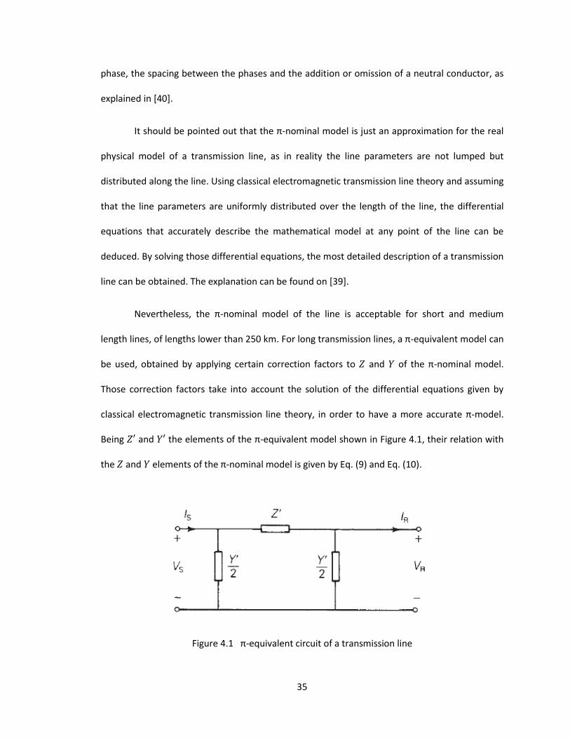
Being 𝑍′ and 𝑌′ the elements of the π-equivalent model shown in Figure 4.1, their relation with

the 𝑍 and 𝑌 elements of the π-nominal model is given by Eq. (9) and Eq. (10).

Figure 4.1 π-equivalent circuit of a transmission line

36

𝑍′ = 𝑍 sinh(𝛾l)

𝛾l (9)

𝑌′ = 𝑌 tanh(

𝛾l2)

𝛾l2

(10)

Where 𝛾 is the propagation constant of the line, defined by Eq. (11):

𝛾 = √𝑧𝑦 (11)

The hyperbolic sine and hyperbolic tangent functions take a value of approximately 1

when the value of 𝑙 is not high, as shown in Figure 4.2. Figure 4.2, where the x-axis range has

been fixed to the typical range for lines shorter than 300 km, is the graphical explanation as to

why the π-nominal model is valid for short and medium length lines.

Figure 4.2 Hyperbolic sine and hyperbolic tangent functions for transmission lines

37

For the work developed in this Chapter, the point of interconnection of the wind farm

with the rest of the system was modified by adding a power transmission line between the wind

farm’s step-up transformer and the rest of the network. This was achieved by adding an extra

transmission line located between bus 25 and bus 37 of the IEEE 39-bus system. Therefore, a

40th bus was added to the system, being the wind farm located in bus 37, its step-up

transformer between buses 37 and 40, and the extra transmission line between buses 40 and

25. In the base case considering the extra line, the per-unit values of 𝑍 and 𝑌 for its π-model

were set equal to the ones corresponding to the line that connects buses 1 and 2 in the 39-bus

system, in order to represent a realistic transmission line. Since the per-length magnitudes 𝑧 and

𝑦 are not available for the 39-bus test case, it is not possible to estimate the real length of the

line. Certain utilities in the New England region were consulted for this study regarding the

generic per-length values of their line parameters, but they were reluctant to provide this

information due to security reasons.

Several cases of the connecting transmission line were considered, each of them

obtained by modifying the 𝑍 and 𝑌 values of the π-model in order to represent increasing line

lengths. For the sake of simplicity, the 𝑍 and 𝑌 values of the π -model were multiplied by the

same constant for each of the cases of extra transmission line considered in this study, in order

to obtain 𝑍’ and 𝑌’. For future studies, given that generic per-length parameters of a

transmission line can be provided by a utility, Eq. (9) and Eq. (10) can be used to calculate the

correction factors for the π-equivalent model.

The phasor diagram in Figure 4.3 represents the different values of the Thevenin

impedance seen by the wind farm bus for the several cases of extra transmission line

considered, each of which was obtained by modifying the values of the π-model parameters as

38

mentioned before. These are per-unit values, being the impedance base used in that bus of 4 Ω.

The power base in the system was 100 MVA and the voltage base in the wind bus was 20 kV.

Figure 4.3 Phasor diagram of the Thevenin impedances seen by the wind farm

4.2 Thevenin Impedance Calculations

The Thevenin impedance is calculated throughout this thesis by using the impedance

matrix of the system, 𝒁𝑏𝑢𝑠, using a procedure detailed in some power system analysis books as

[41]. The procedure is summarized is this Section.

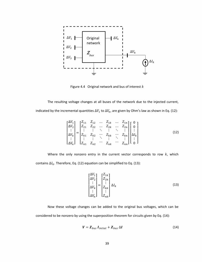
Figure 4.4 shows a general power system where 𝑘 is the bus of interest for calculating

the Thevenin equivalent. Initially, let the circuit not be energized so that the bus currents and

voltages are zero. Then, a current of ∆𝐼𝑘 (in amp or per-unit) is injected from bus 𝑘 into the

system through a current source connected to the voltage reference node, causing a ∆𝑉 in every

bus of the system.

39

Figure 4.4 Original network and bus of interest 𝑘

The resulting voltage changes at all buses of the network due to the injected current,

indicated by the incremental quantities ∆𝑉1 to ∆𝑉𝑛, are given by Ohm’s law as shown in Eq. (12):

[ ∆𝑉1

∆𝑉2

⋮∆𝑉𝑘

⋮∆𝑉𝑛]

=

[ 𝑍11

𝑍21

⋮𝑍𝑘1

⋮𝑍𝑛1

𝑍12

𝑍22

⋮𝑍𝑘2

⋮𝑍𝑛2

⋯⋯⋱⋯⋱⋯

𝑍1𝑘

𝑍2𝑘

⋮𝑍𝑘𝑘

⋮𝑍𝑛𝑘

⋯⋯⋱⋯⋱⋯

𝑍1𝑛

𝑍2𝑛

⋮𝑍𝑘𝑛

⋮𝑍𝑛𝑛]

[

00⋮

∆𝐼𝑘⋮0 ]

(12)

Where the only nonzero entry in the current vector corresponds to row 𝑘, which

contains ∆𝐼𝑘. Therefore, Eq. (12) equation can be simplified to Eq. (13):

[ ∆𝑉1

∆𝑉2

⋮∆𝑉𝑘

⋮∆𝑉𝑛]

=

[ 𝑍1𝑘

𝑍2𝑘

⋮𝑍𝑘𝑘

⋮𝑍𝑛𝑘]

∆𝐼𝑘 (13)

Now these voltage changes can be added to the original bus voltages, which can be

considered to be nonzero by using the superposition theorem for circuits given by Eq. (14):

𝑽 = 𝒁𝑏𝑢𝑠 𝑰𝑖𝑛𝑡𝑖𝑎𝑙 + 𝒁𝑏𝑢𝑠 ∆𝑰 (14)

∆𝑉1

∆𝑉2

∆𝑉𝑛 Original network

Zbus

∆𝑉𝑘

∆𝑉3 ∆𝐼𝑘

40

Where 𝑽 is the bus voltages vector, 𝑰𝑖𝑛𝑡𝑖𝑎𝑙 is the initial injected currents vector and ∆𝑰 is

the vector of injected currents changes.

Therefore, the equation for the voltage at bus 𝑘 comes up to be:

𝑉𝑘 = 𝑉𝑘𝑖𝑛𝑖𝑡𝑖𝑎𝑙 + 𝑍𝑘𝑘 ∆𝐼𝑘 (15)

The circuit corresponding to Eq. (15) is shown in Figure 4.5, from where it can be

deduced that the Thevenin impedance at a particular bus 𝑘 of the system is given by:

𝑍𝑇ℎ𝑒𝑣 = 𝑍𝑘𝑘 (16)

Figure 4.5 Thevenin equivalent circuit at bus 𝑘

Where 𝑍𝑘𝑘 is the diagonal component in row 𝑘 and column 𝑘 of the impedance matrix

of the system, 𝒁𝑏𝑢𝑠.

The values of the Thevenin impedance seen by the wind bus that are represented in

Figure 4.3 were calculated using this procedure.

𝑉𝑘

∆𝐼𝑘 +

- 𝑉𝑘

𝑖𝑛𝑖𝑡𝑖𝑎𝑙

Original network

Zbus

𝑍𝑇ℎ𝑒𝑣 = 𝑍𝑘𝑘

41

4.3 Fixed Fault Duration

For each of these cases of transmission line connecting the wind farm shown in 4.3, a

three-phase-to-ground, 0.25-second-long fault was applied in every bus of the system, while the

wind farm was located in bus 37. The duration of the fault corresponds to the backup clearing

time for protection relays in some power systems. Time-domain simulations were conducted,

and the voltage performance of every bus in the system was analyzed. After the fault was

cleared, peaks in the wind bus and near buses could be observed, similar to the ones in Figure

3.1.

The relation between the Thevenin reactance, 𝑋𝑇ℎ𝑒𝑣, and the magnitudes that

characterize the fault effects is presented from Figure 4.6 through Figure 4.8 for faults located in

three of the system buses. These are just three examples out of the forty obtained, as a fault

was placed in every bus of the system. Every bus showed a similar behavior to the ones included

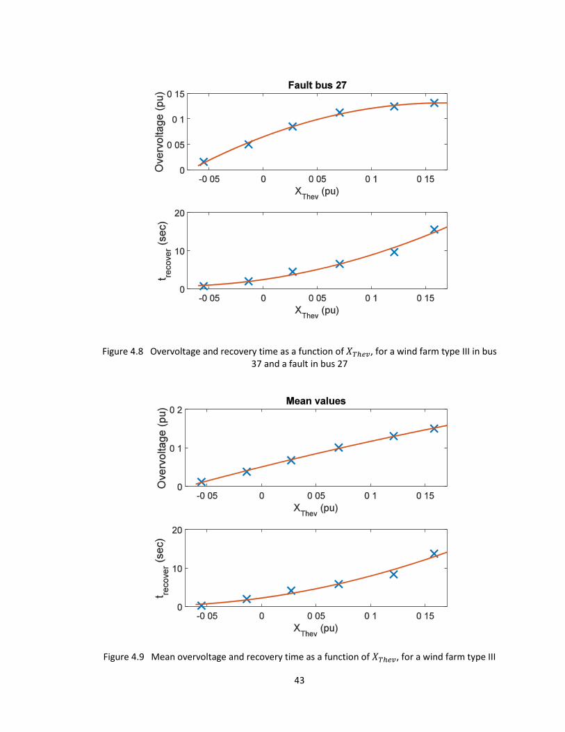
in these plots, thus Figure 4.6 through Figure 4.8 give the reader a good idea of the general

trend. Figure 4.9 includes the mean values for all fault locations in the system.

The upper plot in Figure 4.6 through Figure 4.9 presents the highest difference between

the post-fault voltage peak and the pre-fault voltage value of that same bus as a function of

𝑋𝑇ℎ𝑒𝑣. This highest voltage difference was in every case seen in the wind farm bus. The lower

plot in Figure 4.6 through Figure 4.9 shows the longest voltage recovery time for any bus in the

system as a function of 𝑋𝑇ℎ𝑒𝑣, which also corresponds in every case to the recovery time of the

wind farm bus. The recovery time is defined in this case as the time it takes the voltage to go

back to ±1% of its pre-fault value. A graphical explanation of the voltage overshoot difference

and recovery time can be found in Figure 2.8. The results shown from Figure 4.6 through Figure

4.9 correspond to the analysis made using a wind type III wind farm.

42

Figure 4.6 Overvoltage and recovery time as a function of 𝑋𝑇ℎ𝑒𝑣, for a wind farm type III in bus

37 and a fault in bus 1

Figure 4.7 Overvoltage and recovery time as a function of 𝑋𝑇ℎ𝑒𝑣, for a wind farm type III in bus 37 and a fault in bus 9

43

Figure 4.8 Overvoltage and recovery time as a function of 𝑋𝑇ℎ𝑒𝑣, for a wind farm type III in bus 37 and a fault in bus 27

Figure 4.9 Mean overvoltage and recovery time as a function of 𝑋𝑇ℎ𝑒𝑣, for a wind farm type III

44

As can be seen from Figure 4.6 through Figure 4.9, both the overvoltage difference and

the recovery time increase as 𝑋𝑇ℎ𝑒𝑣 increases, meaning that the increase in length of the

connecting transmission line deteriorates the dynamic voltage performance of the system. The

plot shows that there is a correlation between these two magnitudes, which characterize the

impact of the fault on the voltage performance of the system, and the Thevenin reactance seen

by the wind farm bus. A second order regression has been plotted on top of the data obtained

from the simulations, showing it to be a good approximation. These results also show that the

interconnection between the wind farm and the rest of the power system plays a significant role

on the effects of a fault on the voltage performance of the system buses, as the dynamic voltage

deterioration is quite significant with an increasing-length line.

The original 39-bus case, in which no additional line was added to connect the wind

farm to the rest of the system, corresponds to the lowest value of 𝑋𝑇ℎ𝑒𝑣 shown in the plots. This

case shows the lowest overvoltage and recovery time, as can be seen from Figure 4.6 through

Figure 4.9. Therefore, another important conclusion can be made by analyzing the plots: the

results of the simulations show that the best option from the voltage performance point of view

for integrating a new wind farm to a power grid consists on connecting it directly to the existing

electric lines to a low Thevenin impedance system node. However, as this might not always be

feasible due to the impossibility of freely choosing the location of a new wind farm, which is

subject to weather and environmental constraints, this analysis shows that the electric line used

for the interconnection should have as small reactance as possible. This can be achieved by the

addition of shunt capacitors at both ends of the transmission line, which would reduce the

effective reactance of the line.

45

All in all, the results show that the Thevenin reactance is a good tool when assessing the

impact of a potential fault on the dynamic voltage performance of the wind bus. The value of

𝑋𝑇ℎ𝑒𝑣 seen by the wind bus can be used, as a first approximation, to predict the severity of a

fault in the wind terminal. This is particularly useful when there are several available options for

connecting a wind farm to a power system. As compared to the Short Circuit Ratio, the main

advantages of the Thevenin impedance are its straight-forward derivation for the impedance

matrix and the easiness of conducting circuit calculations by using the Thevening equivalent.

This equivalent circuit can provide a simple theoretical explanation to the causes of voltage

deterioration in each case.

The dynamic voltage performance observed in Chapter 3, and Figure 4.6 through Figure

4.9, raises a question about overvoltage regulations in power systems. Institutions such as the

North American Electric Reliability Corporation (NERC) have thoroughly studied low-voltage-

ride-through characteristics of wind turbines, and developed standards that utilities must follow

to maintain stability in their systems. However, high-voltage regulation has not been paid much

attention to. The present work shows that there is a need for a deeper knowledge of power

system overvoltages, and agencies like NERC should consider developing standards that regulate

them in order to ensure power quality in North America.

The plots from Figure 4.6 through Figure 4.8 show another interesting fact: both the

overvoltage and recovery time of the wind bus can be fairly well approximated by a 2nd order

polynomial, as mentioned before. In order to check the goodness of the polynomial fit for a fault

in any bus of the system, the R-squared of the simulation samples with respect to the

polynomial fit was calculated. The R-squared, or R2, is a number between 0 and 1 that indicates

how well a statistical model fits a set of data. An R2 of 1 indicates that the model perfectly fits

46

the data, while an R2 of 0 indicates that the model does not fit the data at all. R2 is defined by

the following equation:

𝑅2 = 1 −𝑅𝑆𝑆

𝑇𝑆𝑆 (17)

TSS is the total sum of squares, defined as the sum over all data samples of the squared

differences of each sample from the overall mean:

𝑇𝑆𝑆 = ∑(𝑦𝑖 − �̅�)2

𝑖

(18)

Where 𝑦𝑖 are the data samples and �̅� is their mean.

𝑅𝑆𝑆 is the residual sum of squares, defined as the sum of the squares of residuals,

which are the deviation of the values predicted by the model from the actual empirical values of

the data:

𝑅𝑆𝑆 = ∑𝑒𝑖2

𝑖

= ∑(𝑦𝑖 − 𝑓𝑖)2

𝑖

(19)

Where 𝑒𝑖 are the residuals and 𝑓𝑖 are the values predicted by the model.

The R-Squared of the simulation data with respect to the 2nd order polynomial fit was

calculated for every fault location. The results can be seen in Figure 4.10 and Figure 4.11.

47

Figure 4.10 R-squared for the overvoltages as a function of 𝑋𝑇ℎ𝑒𝑣, for a wind farm type III

Figure 4.11 R-squared for the recovery time as a function of 𝑋𝑇ℎ𝑒𝑣, for a wind farm type III

48

These plots show that the accuracy of the fit is over 95% for most buses except for bus

25 for the overvoltage regression and bus 37 for the recovery time regression, both having a

significantly poorer accuracy. Bus 37 corresponds to the wind farm bus, and bus 25 is the bus

that connects the extra transmission line to the rest of the system. The likely reason for these

buses not following the 2nd order trend that other buses do is their proximity to the wind

controller, which has a much more significant control capability when the fault is located near it.

However, when the fault is further from the wind bus, the wind controller does not have such a

significant influence, and the dynamics of the whole system play an important role too.

The high accuracy of the 2nd order regression for every bus in the system located within

a certain distance of the wind bus is interesting for several reasons. On the one hand, a parabola

is a very convenient description for conducting mathematical manipulations, so having such

relationship between the magnitude that characterizes a transmission line and the magnitudes

that characterize the effect of a fault can open new theoretical studies on the matter.

Furthermore, it is surprising to realize that such a complex system as a power grid, which is

overall a very convoluted physical model due to all the dynamics of the different devices it is

composed of, can be represented by a mathematical expression as simple as a 2nd order

polynomial. The theory behind this parabola correlation could be considered as a topic for

future studies.

The relation between the Thevenin reactance, 𝑋𝑇ℎ𝑒𝑣, and the magnitudes that

characterize the impact of a fault was also determined for a type IV wind farm. Figure 4.12

through Figure 4.14 present this relation for three of the system buses.

49

Figure 4.12 Overvoltage and recovery time as a function of 𝑋𝑇ℎ𝑒𝑣, for a wind farm type IV in bus 37 and a fault in bus 5

Figure 4.13 Overvoltage and recovery time as a function of 𝑋𝑇ℎ𝑒𝑣, for a wind farm type IV in bus 37 and a fault in bus 15

50

Figure 4.14 Overvoltage and recovery time as a function of 𝑋𝑇ℎ𝑒𝑣, for a wind farm type IV in bus 37 and a fault in bus 28

Only four samples of the Thevenin reactance can be seen in these plots, when

compared to the six samples shown in the corresponding type III plots. The two highest values

of 𝑋𝑇ℎ𝑒𝑣 are not included in the plots due to singularity issues that arose when conducting time-

domain simulations using the type IV wind turbine model. For the fault located in certain buses,

the Jacobian of the state matrix of the system, which is computed during the time-domain

simulation in order to solve for the values of the state variables in each time step, became

singular. This issue could be solved by increasing the fault impedance, but doing so was

inaccurate for this study since only three-phase-to-ground faults are considered. Therefore, if

the faulted bus voltage does not reach a value close to 0 per-unit due to an excessively high

fault impedance, the simulation cannot be considered valid for this analysis. The singularity

issues were particularly significant for the two highest values of 𝑋𝑇ℎ𝑒𝑣, for which several buses

51

in the system incurred in singularities, and therefore those values of 𝑋𝑇ℎ𝑒𝑣 had to be left out of

the study.

The R-squared analysis for the 2nd order polynomial fit of all the system buses when

considering a type IV wind turbine is presented in Figure 4.15 and Figure 4.16. The missing

samples in the plots correspond to buses which incurred in singularities.

Figure 4.15 R-squared for the overvoltages as a function of 𝑋𝑇ℎ𝑒𝑣, for a wind farm type IV

52

Figure 4.16 R-squared for the recovery time as a function of 𝑋𝑇ℎ𝑒𝑣, for a wind farm type IV

Although the accuracy of the 2nd order regression is also very high, the result is not as

significant as for type III, since in this case some buses and some values of 𝑋𝑇ℎ𝑒𝑣 had to be left

out of the analysis.

Due to the disappointing simulation performance of the PSAT type IV model, a literature

review was conducted, in search of studies mentioning similar issues. Some, such as [42], have

pointed out discrepancies seen in the results from different transient stability software

packages, which may give substantially different results for very similar system models.

Reference [42] deals with developing validation methodologies for different simulation

packages. In addition, other studies have proposed the use of alternative dynamic models for

systems with weak grids, since they consider that certain simplifications in the model should not

be made for these cases [24], [43]. As wind integration studies usually fall under this category of

weak systems, due to the long transmission lines typically needed to connect the wind farm to

53

the rest of the network, the dynamic models developed in studies such as the ones cited should

be getting more attention.

Therefore, this study concludes that further investigation regarding the dynamic model

of type IV wind turbines is needed, and should particularly be brought to the attention of PSAT

developers.

4.4 Increasing Fault Duration

For concluding the study about the influence of the wind farm point of interconnection,

the impact of the fault duration was analyzed. The same six cases of connecting transmission

line as in the previous Sections were considered, as shown in the phasor diagram in Figure 4.3,

and for each of them a fault was placed in three of the system buses and its duration was

sequentially increased. The three fault locations selected were bus 11, a bus far from the wind

farm; bus 17, a bus within middle distance of the wind farm; and bus 26, a bus close to the wind

farm. The results can be observed from Figure 4.17 through Figure 4.19, all of which consider a

type III wind farm. This study was not conducted for a type IV wind farm due to the singularity

issues encountered in Section 4.3.

Figure 4.17 through Figure 4.19 present the magnitudes that characterize the severity of

the fault, both the voltage overshoot and the recovery time, as a function of the fault duration.

The several cases of connecting line length are represented using different colors for the curves.

The legend entries for each of the curves, Z1 to Z6, represent increasing length of the

connecting transmission line, where Z1 corresponds to the original case with no extra line and

Z6 corresponds to the longest line considered. The increasing values of Z also correspond to

increasing values of 𝑋𝑇ℎ𝑒𝑣 because, as explained in previous Sections, 𝑋𝑇ℎ𝑒𝑣 increases with line

length.

54

Figure 4.17 Overvoltage and recovery time as a function of fault duration, for a wind farm type III in bus 37 and a fault in bus 11

Figure 4.18 Overvoltage and recovery time as a function of fault duration, for a wind farm

type III in bus 37 and a fault in bus 17

55

Figure 4.19 Overvoltage and recovery time as a function of fault duration, for a wind farm type III in bus 37 and a fault in bus 26

These plots show that the combined effect of an increasing value of 𝑋𝑇ℎ𝑒𝑣 and

increasing fault duration can have severe effects on the dynamic voltage performance of the

system. One important conclusion can be made from these results: the clearing time of a fault is

particularly important for cases in which a long transmission line is used to connect the wind

farm to the system. Therefore, utilities would have to make a higher investment in fast-

actuating protection relays for their grid in case they have a weak wind farm connection. An

analysis of the best option from an economical point of view should be made by the utility in

such a case, as it might be less expensive to invest in improving the transmission grid rather than

in state-of-the-art protection relays.

56

CHAPTER 5

CONCLUSIONS AND FUTURE WORK

In the present thesis, the IEEE 39-bus test case has been used to develop a methodology

to study dynamic voltage characteristics of a power system with wind penetration. This work

has set the base for extending the analysis to the real New England power system.

One of the contributions of this thesis is the code developed for automating the

simulations and the analysis of its results, as it will be available to future students conducting

power system analysis with PSAT. This code could potentially be included in the PSAT library as

an additional functionality of the toolbox, so that all its users can benefit from it, therefore

contributing to the philosophy of open-source freeware as PSAT.

The dynamic voltage performance observed in Chapters 3 and 4 raises a question about

overvoltage regulations in power systems. Institutions such as NERC have thoroughly studied

low-voltage-ride-through characteristics of wind turbines, and developed standards that utilities

must follow to maintain stability in their systems. However, high-voltage regulation has not

been paid much attention to. This thesis shows that there is a need for a deeper knowledge of

power system overvoltages. It is important to mention that the voltage overshoot following the

fault clearing is directly linked with the voltage regulators of the generators, and this work

considered a constant excitation for the synchronous machines. As future work to expand the

study presented in this thesis, a more detailed model of the voltage regulators can be

considered. This future study will show if the overshoots are a still a concern, and if they should

be brought to the attention of regulation agencies as NERC.

57

One of the goals of this thesis was to shed some light on the not very well studied type

IV wind turbines. The singularity issues encountered when conducting time-domain simulations

using this type of wind turbine show that further study is needed regarding its modelling, and

particularly the PSAT model for it should be further validated.

The analysis of the simulations conducted in Chapter 4 shows that the interconnection

between the wind farm and the rest of the power system plays a significant role on the

effects of a fault on its voltage performance. The Thevenin reactance seen by the wind

bus, a concept not explicitly used before in dynamic voltage studies, has been proved to

be a good tool when assessing the impact of a fault on the system. The Thevenin

reactance is particularly useful when there are several available options for connecting a

wind farm to a power system. In addition, it was shown that a 2nd order polynomial can

represent with a high level of accuracy the relation between the magnitudes that

characterize the severity of the fault and the Thevenin reactance seen by the wind bus,

for every bus in the system located within a certain distance of the wind bus.

Chapter 4 has also shown that the combined effect of a long transmission line

connecting the wind farm to the system and increasing fault duration can have severe effects on

the dynamic voltage performance of the network. Therefore, an analysis of the best option from

an economical point of view should be made on a case-to-case basis between improving the

electrical connection of the wind farm and installing fast-actuating protection relays.

Regarding future work, the main goal should be to extend the present study to the real

New England power grid. As a first step, a study using a more detailed modeling of synchronous

machines which includes automatic voltage regulators should be conducted. For this work, it is

58

recommended to make use of a bigger test case than the 39-bus system, as it would allow

analyzing the behavior of wind farms in a bigger power system.

In addition, the different voltage control scheme of the PSAT type III and type IV models

should be further investigated, as has been identified as the cause of the worse performance

shown by type IV in Chapters 3 and 4. It should also be studied to what extent these control

schemes can be modified, as they do not only depend on the structure of the voltage controller,

but also on the 𝑄 output of the machine, which is partially determined by the inherent physical

characteristics of each type of turbine.

Finally, the study on the influence of the wind farm point of interconnection could be

expanded to consider offshore wind farms, given the distinctive characteristics of the

connecting subsea cable and their recent increase in popularity.

59

REFERENCES

[1] "The Status of Renewable Electricity Mandates in the States," Report by the Institute for Energy Research, 2011.

[2] "Global Wind Report Annual Market Update," Report by the Global Wind Energy Council, 2014.

[3] M. Henderson, W. Henson, J. Norden, W. Coste, R. Zavadil, R. Piwko, G. Jordan, G. Hinkle and N. Miller, "ISO New England Wind Integration Study," Proceedings of the IEEE PES General Meeting, 2011.

[4] "ISO New England’s Resource Mix," [Online]. Available: http://www.iso-ne.com/about/what-we-do/key-stats/resource-mix. [Accessed November 2015].

[5] "Maine Renewable Electricity Mandate Status," Report by the Institute for Energy Research, 2010.

[6] J. W. Feltes, B. S. Fernandes and P. K. Keung, "Case Studies of Wind Park Modeling," Proceedings of the IEEE PES General Meeting, 2011.

[7] H. Jiang, Y. Zhang, J. J. Zhang, D. W. Gao and E. Muljadi, "Synchrophasor-Based Auxiliary Controller to Enhance the Voltage Stability of a Distribution System With High Renewable Energy Penetration," IEEE Transactions on Smart Grid, vol. 6, no. 4, pp. 2107-2115, 2015.

[8] Y. Chi, Y. Liu, W. Wang and H. Dai, "Voltage Stability Analysis of Wind Farm Integration into Transmission Network," Proceedings of the International Conference on Power System Technology, 2006.

[9] H. T. Le and S. Santoso, "Analysis of Voltage Stability and Optimal Wind Power Penetration Limits for a Non-radial Network with an Energy Storage System," Proceeding of the IEEE PES General Meeting, 2007.

[10] A. Teninge, D. Roye, S. Bacha and J. Duval, "Low voltage ride-through capabilities of wind plant combining different turbine technologies," Proceeding of the European Conference on Power Electronics and Applications, 2009.

[11] M. Ntshangase, S. K. Kariuki, S. Chowdhury and S. P. Chowdhury, "Voltage Stability Analysis of Electricity Networks with DFIG-based Wind Power Plants," Proceedings of the IEEE PES General Meeting, 2012.

[12] L. Peng, Y. Li and B. Francois, "Dynamic Behavior of Doubly Fed Induction Generator Wind Turbines under Three-phase Voltage Dips," Proceedings of the Power Electronics and Motion Control Conference, 2009.

60

[13] F. Mwasilu, J. J. Justo, K. s. Ro and J. w. Jung, "Improvement of dynamic performance of doubly fed induction generator-based wind turbine power system under an unbalanced grid voltage condition," IET Renewable Power Generation, vol. 6, pp. 424 - 434, 2012.

[14] L. Meegahapola, D. Flynn and T. Littler, "Transient Stability Analysis of a Power System with High Wind Penetration," Proceedings of the Universities Power Engineering Conference, 2008.

[15] J. G. Slootweg, "Wind Power Modelling and Impact on Power System Dynamics," PhD Dissertation, Delft University of Technology (Netherlands), 2003.

[16] V. Akhmatov, "Analysis of dynamic behavior of electric power systems with large amount of wind power," PhD Dissertation, Technical University of Denmark, 2003.

[17] L. Jianlin, H. Xiangtao and X. Honghua, "Study on Low Voltage Ride Through Characteristic of Full Power Converter Direct-Drive Wind Power System," Proceedings of the Power Electronics and Motion Control Conference, 2009.

[18] P. Pourbeik, R. J. Koessler, D. L. Dickmander and W. Wong, "Integration of Large Wind Farms into Utility Grids (Part 2 - Performance Issues)," Proceedings of the IEEE PES General Meeting, 2003.

[19] M. E. Haque, K. M. Muttaqi and M. Negnevitsky, "Control of a Stand Alone Variable Speed Wind Turbine with a Permanent Magnet Synchronous Generator," Proceedings of the IEEE Power and Energy Society General Meeting, 2008.

[20] Y. Liyong, Y. Peie, C. Zhenguo, C. Zhigang and L. Zhengxi, "A Novel Control Strategy of Power Converter Used To Direct Driven Permanent Magnet Wind Power Generation System," Proceedings of the International Conference on Power Electronics and Intelligent Transportation System, 2009.

[21] X. Yang, L. Li and F. Jiang, "A Control Strategy Combining Sliding Mode Controller with Crowbar Circuit for Low Voltage Ride Through of Direct-Drive Wind Power System," Proceedings of the IET Renewable Power Generation Conference, 2013.

[22] R. Piwko, N. Miller, J. Sanchez-Gasca, X. Yuan, R. Dai and J. Lyons, "Integrating Large Wind Farms into Weak Power Grids with Long Transmission Lines," Proceedings of the Power Electronics and Motion Control Conference, 2006.

[23] F. Sulla, J. Svensson and O. Samuelsson, "Wind Turbines Voltage Support in Weak Grids," Proceedings of the IEEE PES General Meeting, 2013.

[24] A. Golieva, "Low Short Circuit Ratio Connection of Wind Power Plants," MSc Thesis, Delft University of Technology (Netherlands), 2015.

61

[25] S. H. Huang, J. Schmall, J. Conto, J. Adams, Y. Zhang and C. Carter, "Voltage Control Challenges on Weak Grids with High Penetration of Wind Generation:," Proceedings of the IEEE PES General Meeting, 2012.

[26] M. Chaudhary, S. M. Brahma and S. J. Ranade, "Validated short circuit modeling of Type 3 Wind Turbine Generator with crowbar protection," Proceedings of the North American Power Symposium, 2013.

[27] O. S. Adio, X. Lin, F. Zhao and Z. Bo, "Short circuit analysis for integration of 10MW Windfarm in Nigeria at the PCC," Proceedings of the IEEE PES General Meeting, 2013.

[28] S. Perez-Londono, L. Rodriguez-Garcia and Y. U. Lopez, "Effects of Doubly Fed Wind Generators on Voltage Stability of Power Systems," Proceedings fo the Transmission and Distribution Latin America Conference and Exposition, 2012.

[29] S. S. Lakshmi, "Voltage Stability Assessment of a Power System Incorporating Wind Turbine Using Power System Analysis Toolbox (Psat)," IOSR Journal of Electrical and Electronics Engineering, vol. 9, pp. 19-25, 2014.

[30] F. Bacha and R. Karoui, "Simulation of a Tunisian Wind Farm of Sidi-Daoud Using PSAT," Proceedings of the Conference on Electrical Engineering and Software Applications, 2013.

[31] S. Kumar, A. Kumar and N. K. Sharma, "Analysis of Power Flow, Continuous Power Flow and Transient Stability of IEEE-14 Bus Integrated Wind Farm Using PSAT," Proceedings of the International Conference on Energy Economics and Environment, 2015.

[32] F. Milano, Documentation for Power System Analysis Toolbox version 2.1.6, 2011.

[33] H. Saadat, "Chapter 3: Generator and Transformer Models; the Per-Unit System," in Power System Analysis, 3rd Edition, PSA Publishing, 2010, pp. 88-89.

[34] H. Saadat, "Chapter 11: Stability," in Power System Analysis, 3rd Edition, PSA Publishing, 2010, pp. 500-503.

[35] "Alternative Energy Tutorials: Syncrhonous Generator," [Online]. Available: http://www.alternative-energy-tutorials.com/wind-energy/synchronous-generator.html. [Accessed March 2016].

[36] T. Ackermann, "Chapter 5: Generators and Power Electronics for Wind Turbines," in Wind Power in Power Systems, 2nd Edition, Wiley, 2012, pp. 88-89.

[37] H. Saadat, "Chapter 1: The Power System and Electric Power Generation," in Power System Analysis, 3rd edition, PSA Publishing, 2010, pp. 26-29.

[38] H. Saadat, "Power System Analysis," in Chapter 2: Basic Principles, 3rd Edition, PSA Publishing, 2010, pp. 66-67.

62

[39] J. D. Glover, M. S. Sarma and T. Overbye, "Chapter 5: Transmission lines, steady-state operation," in Power System Analysis and Design, 5th Edition, Cengage Learning, 2012, pp. 249-249.

[40] J. D. Glover, M. S. Sarma and T. Overbye, "Chapter 4: Transmission Line Parameters," in Power System Analysis and Design, 5th Edition, Cenage Learning, 2012.

[41] J. J. Grainger and W. D. Stevenson, "Chapter 8: The Impedance Model and Network Calculations," in Power System Analysis, 1st Edition, McGraw-Hill, 1994, pp. 287-289.

[42] K. S. Shetye, "Validation of Power System Transient Stability Results," MS Thesis, University of Illinois at Urbana-Champaign, 2011.

[43] J. W. Feltes and B. S. Fernandes, "Wind Turbine Generator Dynamic Performance with Weak Transmission Grids," Proceedings of the IEEE PES General Meeting, 2012.

63

BIOGRAPHY OF THE AUTHOR

Luis Badesa was born in Calatayud (Spain) in 1992. He attended high school at IES

Leonardo de Chabacier, graduating with honors. He obtained his Bachelor of Science in

Industrial Engineering from the University of Zaragoza in 2014, with a concentration in

Mechatronics. He joined the Smart Grid Lab at the University of Maine in 2014, as one of the

recipients of the Iberdrola Scholarships for Postgraduate Studies in the US. He authored the

paper “Impact of Wind Generation on Dynamic Voltage Stability and Influence of the Point of

Interconnection”, which was presented in the 2016 IEEE GreenTech Conference, and co-

authored the paper “Monitoring Power System Transient Stability Using Synchrophasor Data”,

which was presented in the 2015 IEEE Power & Energy Society General Meeting. He is a student

member of IEEE Power & Energy Society, as well as a member of Tau Beta Pi, Eta Kappa Nu and

Golden Key.

He is a candidate for the Master of Science degree in Electrical Engineering from the

University of Maine in May 2016.