Implementing cryptographic pairings: a magma tutorial Luis J Dominguez Perez , Ezekiel J Kachisa , and Michael Scott. School of Computing Dublin City University Ireland [email protected][email protected][email protected]Abstract. In this paper we show an efficient implementation of the Tate, ate and R-ate pairings in magma. This will be demonstrated by using the KSS curves with embedding degree k = 18. 1 Introduction One of the first well known applications of cryptographic pairings is the transfor- mation of an elliptic curve discrete logarithm problem (ECDLP) instance into an instance of discrete logarithm problem (DLP) in the finite field. This was done by Menezes, Okamoto and Vanstone [32] by using the Weil pairing while later Frey and R¨ uck [18] also presented a similar technique using the Tate pairing. These applications were examples of a “negative” use of pairings in ECC. How- ever, recently pairing implementations had been created for more constructive uses. Joux [26] showed how pairings can be used for a tripartite authentication protocol. This opened the flood gates for the positive applications of pairings. Shamir [41] for example in 1984 posed as a challenge the concept of an Identity- Based Encryption scheme. Boneh and Franklin [9] proposed a solution to this challenge based on a bilinear map using the Weil pairing. Many more state- of-the-art protocols using bilinear pairings were proposed such as short digital signatures [10]. In response, novel constructions of non-supersingular pairing-friendly ellip- tic curves have been proposed by different authors for pairing based protocols. With constructions such as MNT [35], Freeman [15], BN [6] one can produce ideal pairing-friendly elliptic curves. These are curves whose group bit length size is equal to the bit length size of the underlying field. The importance and effectiveness of such curves is mainly felt in the costs incurred in the compu- tation of pairings. Some of these curves also support twists of higher order, for example sextic twists on the BN curves. Then there are pairing-friendly elliptic curves which are near-ideal. For instance curves as proposed by Barreto, Lynn This author acknowledge support from the Consejo Nacional de Ciencia y Tecnolog´ ıa These authors acknowledge support from the Science Foundation Ireland under Grant No. 06/MI/006
Transcript
Implementing cryptographic pairings:a magma tutorial
Luis J Dominguez Perez?, Ezekiel J Kachisa??, and Michael Scott.??
Abstract. In this paper we show an efficient implementation of theTate, ate and R-ate pairings in magma. This will be demonstrated byusing the KSS curves with embedding degree k = 18.
1 Introduction
One of the first well known applications of cryptographic pairings is the transfor-mation of an elliptic curve discrete logarithm problem (ECDLP) instance into aninstance of discrete logarithm problem (DLP) in the finite field. This was doneby Menezes, Okamoto and Vanstone [32] by using the Weil pairing while laterFrey and Ruck [18] also presented a similar technique using the Tate pairing.These applications were examples of a “negative” use of pairings in ECC. How-ever, recently pairing implementations had been created for more constructiveuses. Joux [26] showed how pairings can be used for a tripartite authenticationprotocol. This opened the flood gates for the positive applications of pairings.Shamir [41] for example in 1984 posed as a challenge the concept of an Identity-Based Encryption scheme. Boneh and Franklin [9] proposed a solution to thischallenge based on a bilinear map using the Weil pairing. Many more state-of-the-art protocols using bilinear pairings were proposed such as short digitalsignatures [10].
In response, novel constructions of non-supersingular pairing-friendly ellip-tic curves have been proposed by different authors for pairing based protocols.With constructions such as MNT [35], Freeman [15], BN [6] one can produceideal pairing-friendly elliptic curves. These are curves whose group bit lengthsize is equal to the bit length size of the underlying field. The importance andeffectiveness of such curves is mainly felt in the costs incurred in the compu-tation of pairings. Some of these curves also support twists of higher order, forexample sextic twists on the BN curves. Then there are pairing-friendly ellipticcurves which are near-ideal. For instance curves as proposed by Barreto, Lynn? This author acknowledge support from the Consejo Nacional de Ciencia y Tecnologıa
?? These authors acknowledge support from the Science Foundation Ireland underGrant No. 06/MI/006
2 Luis J Dominguez Perez, Ezekiel J Kachisa, and Michael Scott.??
and Scott [4], and later as generalised by Brezing and Weng [12], and KSS curvesas proposed in [27]. In these curves the bit size of the finite field is somewhatlarger compared to the bit size of the prime order subgroup. As such there isalways a need to look for optimal ways to implement pairings on such curves.
The computation of pairings basically involves two groups, G1 and G2. Thesetwo groups are finite cyclic additively-written groups and at least one of whichis of prime order r. The pairing will take an element from each of the two groupsand map them to the third group GT , which is a finite cyclic multiplicatively-written group also of prime order r. A useful cryptographic pairing satisfies thefollowing properties:
– Bilinearity :For all P, P ′ ∈ G1 and all Q,Q′ ∈ G2, one has: e(P + P ′, Q) = e(P,Q)×e(P ′, Q) and e(P,Q+Q′) = e(P,Q)× e(P,Q′)
– Non-degeneracy :For all P ∈ G1 with P 6= 0, there is some Q ∈ G2 such that e(P,Q) 6= 1.For all Q ∈ G2 with Q 6= 0, there is some P ∈ G1 such that e(P,Q) 6= 1.
– Computable:e can be easily evaluated.
The best known method for computing pairings is based on Miller’s algo-rithm. This is a standard method and many researchers have been trying toimprove its efficiency. The emphasis mainly has been to optimize the Miller’sloop and the final exponentiation in the algorithm [ [3], [1], [14], [31], [38],[5],[22]].
Our implementation uses the Magma software package which is a large, well-supported package designed to solve computationally hard problems in algebra,number theory, geometry and combinatorics [11]. Magma currently has internalfunctions to compute the Weil or Tate pairing. However one can also implementthe computation of the pairings using ones own functions to eliminate unneces-sary operations and to exploit specific properties of the chosen family of curvesfor an efficient implementation.
In this paper we will demonstrate using magma a step-by-step approach tothe efficient implementation of pairings given a family of pairing friendly ellipticcurves, and propose some specific optimisations for the chosen k = 18 family ofsuch curves in the computation of the Tate, ate and R-ate pairings.
1.1 Organisation of the paper
The rest of the paper is organised as follows: the next section explains the KSScurves, in particular a family of curves of embedding degree, k = 18. In Section§3 we discuss the twists in elliptic curves and how to create sextic twist curvesin magma. In §4 we discuss how to compute the Tate pairing in Magma forcurves of degree 18, similarly in sections §5 and §6 for the ate pairing and R-atepairing respectively. In §7 we compare the Miller loop length as experienced insections §4, §5 and §6. Finally, in §8 and §9 we discuss an optimisation of thefinal exponentiation in the pairing computations. We conclude our discussionsin §10. Appendix §A illustrates how to count points on the elliptic curve over an
Implementing Cryptographic pairings: a magma tutorial 3
extension field and over a twist of a curve. Appendix §B shows how to generatethe Ti pairs for the R-ate paring.
2 Kachisa-Schaefer-Scott Curves
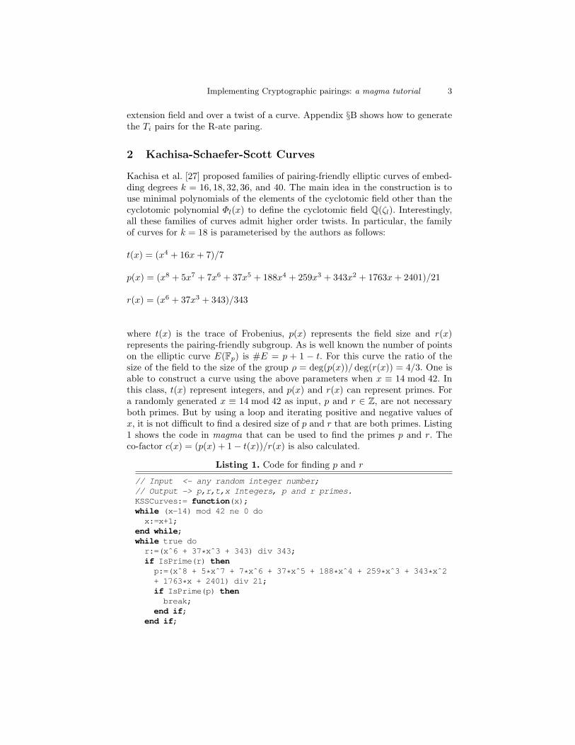
Kachisa et al. [27] proposed families of pairing-friendly elliptic curves of embed-ding degrees k = 16, 18, 32, 36, and 40. The main idea in the construction is touse minimal polynomials of the elements of the cyclotomic field other than thecyclotomic polynomial Φl(x) to define the cyclotomic field Q(ζl). Interestingly,all these families of curves admit higher order twists. In particular, the familyof curves for k = 18 is parameterised by the authors as follows:
where t(x) is the trace of Frobenius, p(x) represents the field size and r(x)represents the pairing-friendly subgroup. As is well known the number of pointson the elliptic curve E(Fp) is #E = p + 1 − t. For this curve the ratio of thesize of the field to the size of the group ρ = deg(p(x))/deg(r(x)) = 4/3. One isable to construct a curve using the above parameters when x ≡ 14 mod 42. Inthis class, t(x) represent integers, and p(x) and r(x) can represent primes. Fora randomly generated x ≡ 14 mod 42 as input, p and r ∈ Z, are not necessaryboth primes. But by using a loop and iterating positive and negative values ofx, it is not difficult to find a desired size of p and r that are both primes. Listing1 shows the code in magma that can be used to find the primes p and r. Theco-factor c(x) = (p(x) + 1− t(x))/r(x) is also calculated.
Listing 1. Code for finding p and r
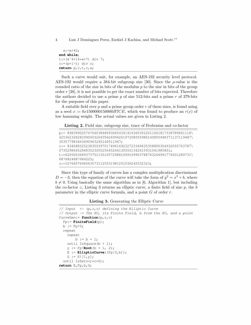
// Input <- any random integer number;// Output -> p,r,t,x Integers, p and r primes.KSSCurves:= function(x);while (x-14) mod 42 ne 0 dox:=x+1;
4 Luis J Dominguez Perez, Ezekiel J Kachisa, and Michael Scott.??
x:=x+42;end while;t:=(xˆ4+16*x+7) div 7;c:=(p+1-t) div r;return p,r,t,c,x;
Such a curve would suit, for example, an AES-192 security level protocol.AES-192 would require a 384-bit subgroup size [30]. Since the ρ-value is therounded ratio of the size in bits of the modulus p to the size in bits of the grouporder r [38], it is not possible to get the exact number of bits expected. Thereforethe authors decided to use a prime p of size 512-bits and a prime r of 379-bitsfor the purposes of this paper.
A suitable field over p and a prime group order r of these sizes, is found usingas a seed x := 0x1500000150000B7CE, which was found to produce an r(x) oflow hamming weight. The actual values are given in Listing 2.
Listing 2. Field size, subgroup size, trace of Frobenius and co-factor
Since this type of family of curves has a complex multiplication discriminantD = −3, then the equation of the curve will take the form of y2 = x3 + b, whereb 6= 0. Using basically the same algorithm as in [6, Algorithm 1], but includingthe co-factor c, Listing 3 returns an elliptic curve, a finite field of size p, the bparameter in the elliptic curve formula, and a point G of order r.
Listing 3. Generating the Elliptic Curve
// Input <- (p,r,c) defining the Elliptic Curve// Output -> The EC, its Finite Field, b from the EC, and a pointCurveGen:= function(p,r,c)Fp:= FiniteField(p);b := Fp!0;repeatrepeat
b := b + 1;until IsSquare(b + 1);y := Fp!Root(b + 1, 2);E := EllipticCurve([Fp|0,b]);G := E![1,y];
until IsZero(r*c*G);return E,Fp,b,G;
Implementing Cryptographic pairings: a magma tutorial 5
Listing 3 begins searching for a curve from b = 1. When one gets to b = 5,that defines an elliptic curve E : y2 = x3 + 21 and a point G(1,
√6) with the
correct order.Although the curve remains defined over Fp, we can also consider points
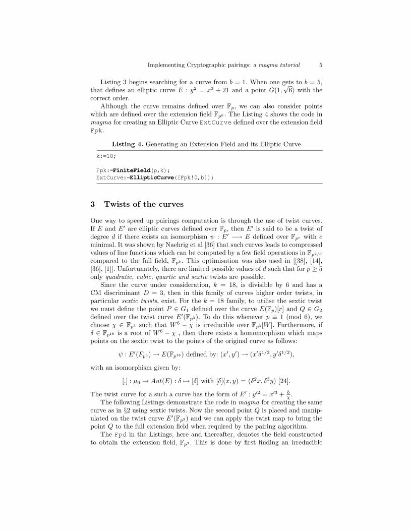
which are defined over the extension field Fpk . The Listing 4 shows the code inmagma for creating an Elliptic Curve ExtCurve defined over the extension fieldFpk.
Listing 4. Generating an Extension Field and its Elliptic Curve
One way to speed up pairings computation is through the use of twist curves.If E and E′ are elliptic curves defined over Fp, then E′ is said to be a twist ofdegree d if there exists an isomorphism ψ : E′ −→ E defined over Fpe with eminimal. It was shown by Naehrig et al [36] that such curves leads to compressedvalues of line functions which can be computed by a few field operations in Fpk/d
compared to the full field, Fpk . This optimisation was also used in [[38], [14],[36], [1]]. Unfortunately, there are limited possible values of d such that for p ≥ 5only quadratic, cubic, quartic and sextic twists are possible.
Since the curve under consideration, k = 18, is divisible by 6 and has aCM discriminant D = 3, then in this family of curves higher order twists, inparticular sextic twists, exist. For the k = 18 family, to utilise the sextic twistwe must define the point P ∈ G1 defined over the curve E(Fp)[r] and Q ∈ G2
defined over the twist curve E′(Fp3). To do this whenever p ≡ 1 (mod 6), wechoose χ ∈ Fp3 such that W 6 − χ is irreducible over Fp3 [W ]. Furthermore, ifδ ∈ Fp18 is a root of W 6 − χ , then there exists a homomorphism which mapspoints on the sextic twist to the points of the original curve as follows:
ψ : E′(Fp3)→ E(Fp18) defined by: (x′, y′)→ (x′δ1/3, y′δ1/2),
The twist curve for a such a curve has the form of E′ : y′2 = x′3 + bχ .
The following Listings demonstrate the code in magma for creating the samecurve as in §2 using sextic twists. Now the second point Q is placed and manip-ulated on the twist curve E′(Fp3) and we can apply the twist map to bring thepoint Q to the full extension field when required by the pairing algorithm.
The Fpd in the Listings, here and thereafter, denotes the field constructedto obtain the extension field, Fp3 . This is done by first finding an irreducible
6 Luis J Dominguez Perez, Ezekiel J Kachisa, and Michael Scott.??
polynomial of degree 3 over Fp. For example, to find the irreducible polynomialu3 + 2 for this extension field, one would use a magma function as follows:IrreduciblePolynomial(Fp,3);.
One can now use this polynomial to create the extension field Fp3 . From thisfield we now look for an element χ such that W 6 − χ is irreducible over Fp3 [W ]in order to find a suitable representation of Fp18 as a sextic extension of Fp3 . Itis necessary to pick the χ value that gives the correct order of the twist curve[6].
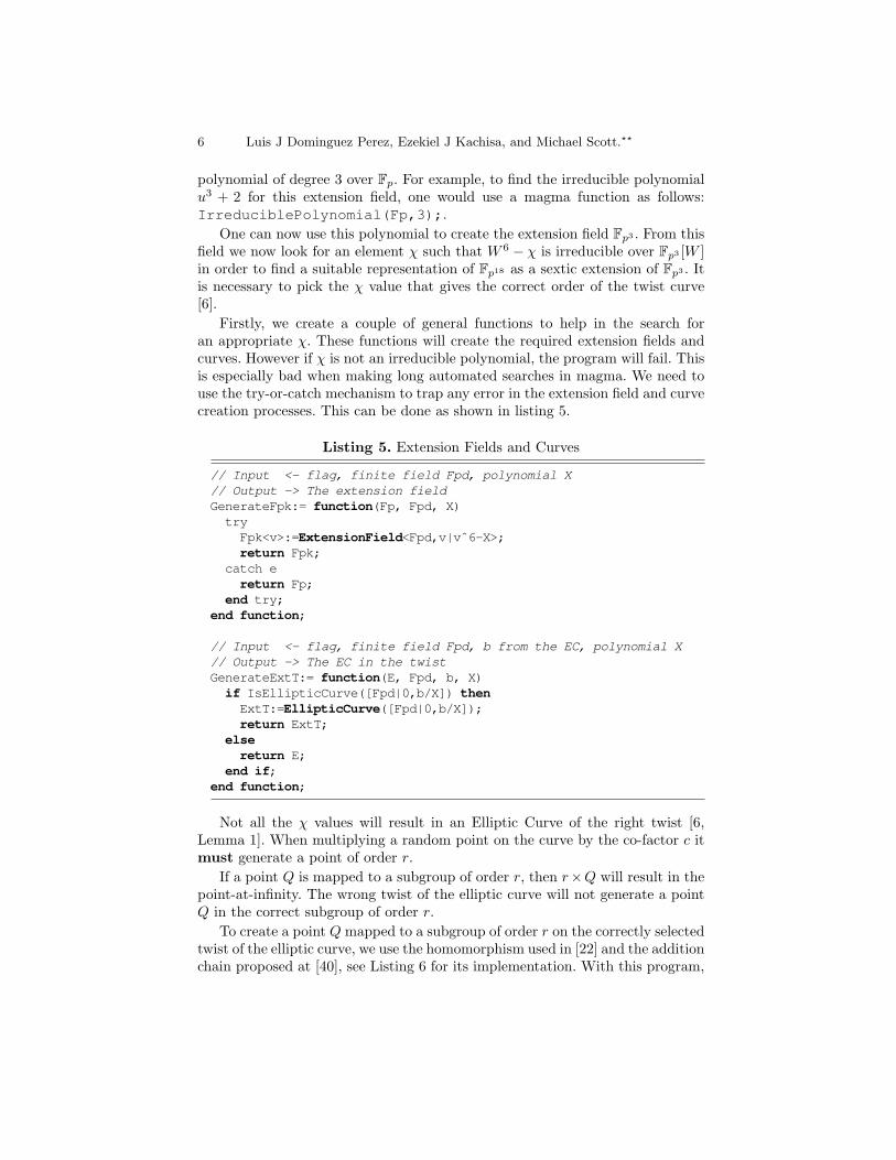
Firstly, we create a couple of general functions to help in the search foran appropriate χ. These functions will create the required extension fields andcurves. However if χ is not an irreducible polynomial, the program will fail. Thisis especially bad when making long automated searches in magma. We need touse the try-or-catch mechanism to trap any error in the extension field and curvecreation processes. This can be done as shown in listing 5.
Listing 5. Extension Fields and Curves
// Input <- flag, finite field Fpd, polynomial X// Output -> The extension fieldGenerateFpk:= function(Fp, Fpd, X)tryFpk<v>:=ExtensionField<Fpd,v|vˆ6-X>;return Fpk;
catch ereturn Fp;
end try;end function;
// Input <- flag, finite field Fpd, b from the EC, polynomial X// Output -> The EC in the twistGenerateExtT:= function(E, Fpd, b, X)if IsEllipticCurve([Fpd|0,b/X]) thenExtT:=EllipticCurve([Fpd|0,b/X]);return ExtT;
elsereturn E;
end if;end function;
Not all the χ values will result in an Elliptic Curve of the right twist [6,Lemma 1]. When multiplying a random point on the curve by the co-factor c itmust generate a point of order r.
If a point Q is mapped to a subgroup of order r, then r×Q will result in thepoint-at-infinity. The wrong twist of the elliptic curve will not generate a pointQ in the correct subgroup of order r.
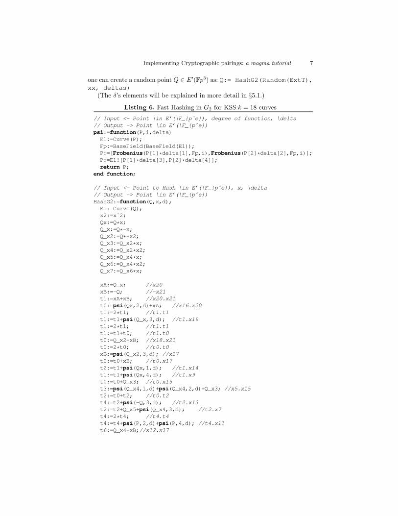
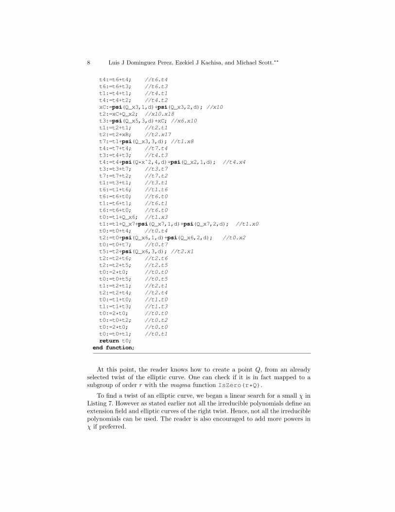
To create a point Q mapped to a subgroup of order r on the correctly selectedtwist of the elliptic curve, we use the homomorphism used in [22] and the additionchain proposed at [40], see Listing 6 for its implementation. With this program,
Implementing Cryptographic pairings: a magma tutorial 7
one can create a random point Q ∈ E′(Fp3) as: Q:= HashG2(Random(ExtT),xx, deltas)
(The δ’s elements will be explained in more detail in §5.1.)
Listing 6. Fast Hashing in G2 for KSS:k = 18 curves
// Input <- Point \in E’(\F_{pˆe}), degree of function, \delta// Output -> Point \in E’(\F_{pˆe})psi:=function(P,i,delta)E1:=Curve(P);Fp:=BaseField(BaseField(E1));P:=[Frobenius(P[1]*delta[1],Fp,i),Frobenius(P[2]*delta[2],Fp,i)];P:=E1![P[1]*delta[3],P[2]*delta[4]];return P;
end function;
// Input <- Point to Hash \in E’(\F_{pˆe}), x, \delta// Output -> Point \in E’(\F_{pˆe})HashG2:=function(Q,x,d);E1:=Curve(Q);x2:=xˆ2;Qx:=Q*x;Q_x:=Q*-x;Q_x2:=Q*-x2;Q_x3:=Q_x2*x;Q_x4:=Q_x2*x2;Q_x5:=Q_x4*x;Q_x6:=Q_x4*x2;Q_x7:=Q_x6*x;
At this point, the reader knows how to create a point Q, from an alreadyselected twist of the elliptic curve. One can check if it is in fact mapped to asubgroup of order r with the magma function IsZero(r*Q).
To find a twist of an elliptic curve, we began a linear search for a small χ inListing 7. However as stated earlier not all the irreducible polynomials define anextension field and elliptic curves of the right twist. Hence, not all the irreduciblepolynomials can be used. The reader is also encouraged to add more powers inχ if preferred.
Implementing Cryptographic pairings: a magma tutorial 9
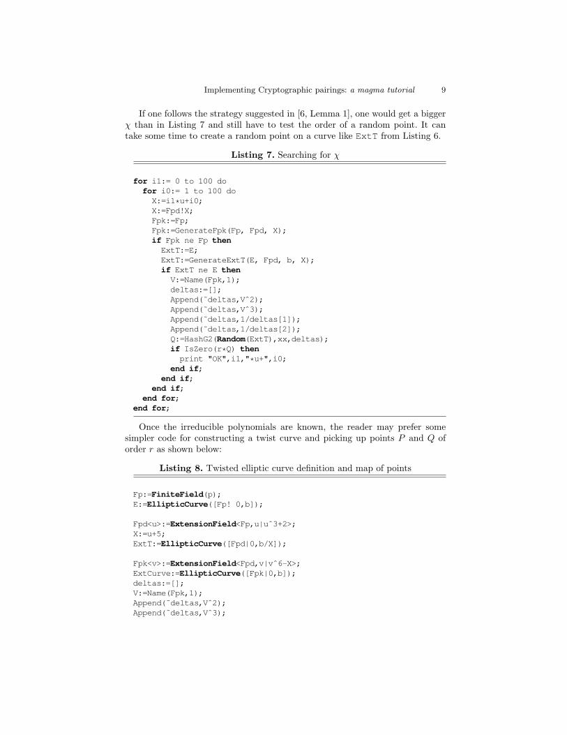
If one follows the strategy suggested in [6, Lemma 1], one would get a biggerχ than in Listing 7 and still have to test the order of a random point. It cantake some time to create a random point on a curve like ExtT from Listing 6.
Listing 7. Searching for χ
for i1:= 0 to 100 dofor i0:= 1 to 100 doX:=i1*u+i0;X:=Fpd!X;Fpk:=Fp;Fpk:=GenerateFpk(Fp, Fpd, X);if Fpk ne Fp thenExtT:=E;ExtT:=GenerateExtT(E, Fpd, b, X);if ExtT ne E thenV:=Name(Fpk,1);deltas:=[];Append(˜deltas,Vˆ2);Append(˜deltas,Vˆ3);Append(˜deltas,1/deltas[1]);Append(˜deltas,1/deltas[2]);Q:=HashG2(Random(ExtT),xx,deltas);if IsZero(r*Q) thenprint "OK",i1,"*u+",i0;
end if;end if;
end if;end for;
end for;
Once the irreducible polynomials are known, the reader may prefer somesimpler code for constructing a twist curve and picking up points P and Q oforder r as shown below:
Listing 8. Twisted elliptic curve definition and map of points
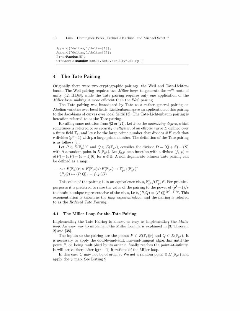
Originally there were two cryptographic pairings, the Weil and Tate-Lichten-baum. The Weil pairing requires two Miller loops to generate the mth roots ofunity [42, III.§8], while the Tate pairing requires only one application of theMiller loop, making it more efficient than the Weil pairing.
The Tate pairing was introduced by Tate as a rather general pairing onAbelian varieties over local fields. Lichtenbaum gave an application of this pairingto the Jacobians of curves over local fields[13]. The Tate-Lichtenbaum pairing ishereafter referred to as the Tate pairing.
Recalling some notation from §2 or [27], Let k be the embedding degree, whichsometimes is referred to as security multiplier, of an elliptic curve E defined overa finite field Fp, and let r be the large prime number that divides #E such thatr divides (pk−1) with p a large prime number. The definition of the Tate pairingis as follows [8]:
Let P ∈ E(Fp)[r] and Q ∈ E(Fpk), consider the divisor D = (Q + S) − (S)with S a random point in E(Fpk). Let fa,P be a function with a divisor (fa,P ) =a(P )− (aP )− (a− 1)(0) for a ∈ Z. A non degenerate bilinear Tate pairing canbe defined as a map:
– er : E(Fp)[r]× E(Fpk)/rE(Fpk)→ F∗pk/(F∗
pk)r
(P,Q) 7→ 〈P,Q〉r = fr,P (D)
This value of the pairing is in an equivalence class, F∗pk/(F∗
pk)r. For practicalpurposes it is preferred to raise the value of the pairing to the power of (pk−1)/rto obtain a unique representative of the class, i.e er(P,Q) = 〈P,Q〉(pk−1)/r. Thisexponentiation is known as the final exponentiation, and the pairing is referredto as the Reduced Tate Pairing.
4.1 The Miller Loop for the Tate Pairing
Implementing the Tate Pairing is almost as easy as implementing the Millerloop. An easy way to implement the Miller formula is explained in [3, Theorem2] and [38].
The inputs to the pairing are the points P ∈ E(Fp)[r] and Q ∈ E(Fpk). Itis necessary to apply the double-and-add, line-and-tangent algorithm until thepoint P , on being multiplied by its order r, finally reaches the point-at-infinity.It will arrive there after lg(r − 1) iterations of the Miller loop.
In this case Q may not be of order r. We get a random point ∈ E′(Fp3) andapply the ψ map. See Listing 9
Implementing Cryptographic pairings: a magma tutorial 11
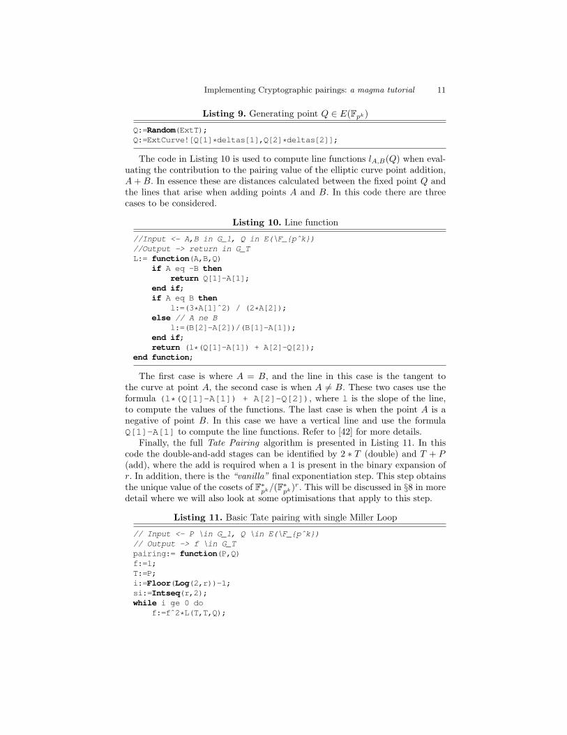
The code in Listing 10 is used to compute line functions lA,B(Q) when eval-uating the contribution to the pairing value of the elliptic curve point addition,A+B. In essence these are distances calculated between the fixed point Q andthe lines that arise when adding points A and B. In this code there are threecases to be considered.
Listing 10. Line function
//Input <- A,B in G_1, Q in E(\F_{pˆk})//Output -> return in G_TL:= function(A,B,Q)
The first case is where A = B, and the line in this case is the tangent tothe curve at point A, the second case is when A 6= B. These two cases use theformula (l*(Q[1]-A[1]) + A[2]-Q[2]), where l is the slope of the line,to compute the values of the functions. The last case is when the point A is anegative of point B. In this case we have a vertical line and use the formulaQ[1]-A[1] to compute the line functions. Refer to [42] for more details.
Finally, the full Tate Pairing algorithm is presented in Listing 11. In thiscode the double-and-add stages can be identified by 2 ∗ T (double) and T + P(add), where the add is required when a 1 is present in the binary expansion ofr. In addition, there is the “vanilla” final exponentiation step. This step obtainsthe unique value of the cosets of F∗
pk/(F∗pk)r. This will be discussed in §8 in more
detail where we will also look at some optimisations that apply to this step.
Listing 11. Basic Tate pairing with single Miller Loop
// Input <- P \in G_1, Q \in E(\F_{pˆk})// Output -> f \in G_Tpairing:= function(P,Q)f:=1;T:=P;i:=Floor(Log(2,r))-1;si:=Intseq(r,2);while i ge 0 do
f:=fˆ2*L(T,T,Q);
12 Luis J Dominguez Perez, Ezekiel J Kachisa, and Michael Scott.??
T:=2*T;if si[i+1] eq 1 then
f:=f*L(T,P,Q);T:=T+P;
end if;i:=i-1;
end while;f:=fˆ(((pˆk)-1) div r);return f;end function;
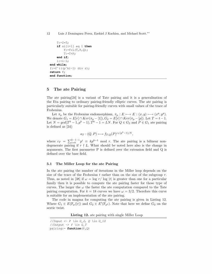
5 The ate Pairing
The ate pairing[24] is a variant of Tate pairing and it is a generalisation ofthe Eta pairing to ordinary pairing-friendly elliptic curves. The ate pairing isparticularly suitable for pairing-friendly curves with small values of the trace ofFrobenius.
Let πp be the Frobenius endomorphism, πp : E 7−→ E : (x, y) 7−→ (xp, yp).We denote G1 = E[r]∩Ker(πp − [1]), G2 = E[r]∩Ker(πp − [p]). Let T = t− 1.Let N = gcd(T k − 1, pk − 1), T k − 1 = LN . For Q ∈ G2 and P ∈ G1 ate pairingis defined as [24]:
aT : (Q,P ) 7−→ fT,Q(P )cT (pk−1)/N ,
where cT =∑k−1−i
i=0 pi ≡ kpk−1 mod r. The ate pairing is a bilinear non-degenerate pairing if r - L. What should be noted here also is the change inarguments. The first parameter P is defined over the extension field and Q isdefined over the base field.
5.1 The Miller Loop for the ate Pairing
In the ate pairing the number of iterations in the Miller loop depends on thesize of the trace of the Frobenius t rather than on the size of the subgroup r.Thus, as noted in [38] if ω = log r/ log |t| is greater than one for a particularfamily then it is possible to compute the ate pairing faster for those type ofcurves. The larger the ω the faster the ate computation compared to the Tatepairing computation. For k = 18 curves we have ω = 3/2. Therefore this curveis suitable for an implementation of the ate pairing.
The code in magma for computing the ate pairing is given in Listing 12.Where G1 ∈ E(Fp)[r]) and G2 ∈ E′(Fp3). Note that here we define G2 on thesextic twist.
Listing 12. ate pairing with single Miller Loop
//Input <- P \in G_2, Q \in G_1$//Output -> f \in G_Tpairing:= function(P,Q)
Implementing Cryptographic pairings: a magma tutorial 13
f:=1;T:=P;s:= t-1;i:=Floor(Log(2,s))-1;si:=Intseq(s,2);while i ge 0 dof:=fˆ2*L(T,T,Q);T:=2*T;if si[i+1] eq 1 thenf:=f*L(T,P,Q);T:=T+P;
end if;i:=i-1;
end while;f:=fˆ(((pˆk)-1) div r);return f;end function;
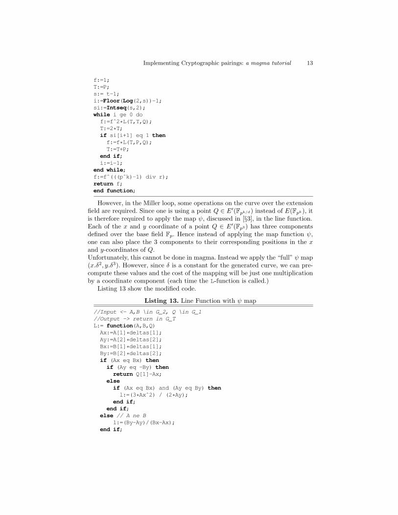
However, in the Miller loop, some operations on the curve over the extensionfield are required. Since one is using a point Q ∈ E′(Fpk/d) instead of E(Fpk), itis therefore required to apply the map ψ, discussed in [§3], in the line function.Each of the x and y coordinate of a point Q ∈ E′(Fp3) has three componentsdefined over the base field Fp. Hence instead of applying the map function ψ,one can also place the 3 components to their corresponding positions in the xand y-coordinates of Q.Unfortunately, this cannot be done in magma. Instead we apply the “full” ψ map(x.δ2, y.δ3). However, since δ is a constant for the generated curve, we can pre-compute these values and the cost of the mapping will be just one multiplicationby a coordinate component (each time the L-function is called.)
14 Luis J Dominguez Perez, Ezekiel J Kachisa, and Michael Scott.??
return (l*(Q[1]-Ax) + Ay-Q[2]);end function;
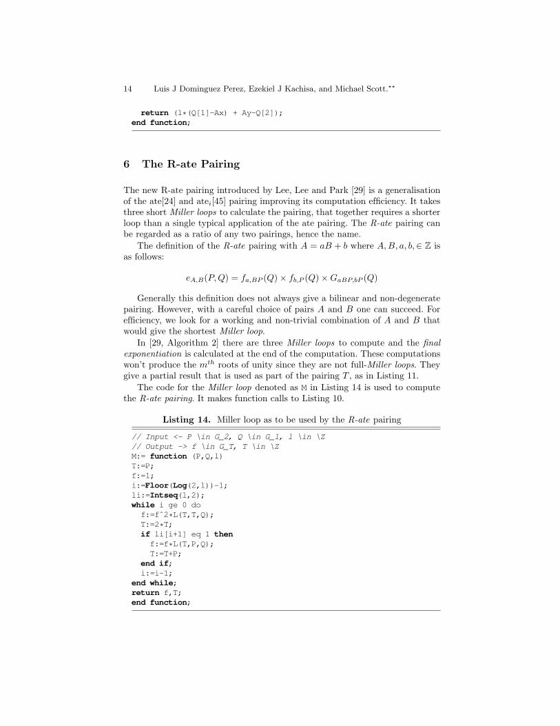
6 The R-ate Pairing
The new R-ate pairing introduced by Lee, Lee and Park [29] is a generalisationof the ate[24] and atei[45] pairing improving its computation efficiency. It takesthree short Miller loops to calculate the pairing, that together requires a shorterloop than a single typical application of the ate pairing. The R-ate pairing canbe regarded as a ratio of any two pairings, hence the name.
The definition of the R-ate pairing with A = aB + b where A,B, a, b,∈ Z isas follows:
eA,B(P,Q) = fa,BP (Q)× fb,P (Q)×GaBP,bP (Q)
Generally this definition does not always give a bilinear and non-degeneratepairing. However, with a careful choice of pairs A and B one can succeed. Forefficiency, we look for a working and non-trivial combination of A and B thatwould give the shortest Miller loop.
In [29, Algorithm 2] there are three Miller loops to compute and the finalexponentiation is calculated at the end of the computation. These computationswon’t produce the mth roots of unity since they are not full-Miller loops. Theygive a partial result that is used as part of the pairing T , as in Listing 11.
The code for the Miller loop denoted as M in Listing 14 is used to computethe R-ate pairing. It makes function calls to Listing 10.
Listing 14. Miller loop as to be used by the R-ate pairing
// Input <- P \in G_2, Q \in G_1, l \in \Z// Output -> f \in G_T, T \in \ZM:= function (P,Q,l)T:=P;f:=1;i:=Floor(Log(2,l))-1;li:=Intseq(l,2);while i ge 0 dof:=fˆ2*L(T,T,Q);T:=2*T;if li[i+1] eq 1 thenf:=f*L(T,P,Q);T:=T+P;
end if;i:=i-1;
end while;return f,T;end function;
Implementing Cryptographic pairings: a magma tutorial 15
There are a few differences between the Listing 11 and Listing 14. In partic-ular the absence of the final exponentiation, the introduction of the parameterl that prescribes the number of loops, instead of r or t-1 and the use of T asan extra output in Listing 14.
The R-ate pairing, like in the atei [45], requires the calculation of Ti ≡ pi modr, with 0 ≤ i < k, where k is the embedding degree. This pairing is constructedfrom the parameters (p, r), which are also used to define the ate and Tate pairing,and a combinations of Ti.
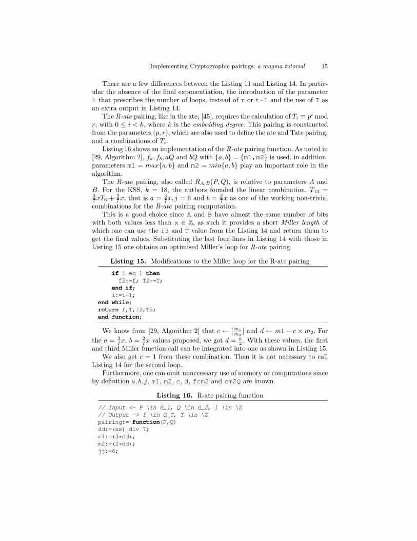
Listing 16 shows an implementation of the R-ate pairing function. As noted in[29, Algorithm 2], fa, fb, aQ and bQ with {a, b} = {m1,m2} is used, in addition,parameters m1 = max{a, b} and m2 = min{a, b} play an important role in thealgorithm.
The R-ate pairing, also called RA,B(P,Q), is relative to parameters A andB. For the KSS, k = 18, the authors founded the linear combination, T13 =37xT6 + 2
7x, that is a = 37x, j = 6 and b = 2
7x as one of the working non-trivialcombinations for the R-ate pairing computation.
This is a good choice since A and B have almost the same number of bitswith both values less than x ∈ Z, as such it provides a short Miller length ofwhich one can use the f3 and T value from the Listing 14 and return them toget the final values. Substituting the last four lines in Listing 14 with those inListing 15 one obtains an optimised Miller’s loop for R-ate pairing.
Listing 15. Modifications to the Miller loop for the R-ate pairing
if i eq 1 thenf2:=f; T2:=T;
end if;i:=i-1;
end while;return f,T,f2,T2;end function;
We know from [29, Algorithm 2] that c ← [m1m2
] and d ← m1 − c ×m2. Forthe a = 3
7x, b = 27x values proposed, we got d = a
2 . With these values, the firstand third Miller function call can be integrated into one as shown in Listing 15.
We also get c = 1 from these combination. Then it is not necessary to callListing 14 for the second loop.
Furthermore, one can omit unnecessary use of memory or computations sinceby definition a, b, j, m1, m2, c, d, fcm2 and cm2Q are known.
Listing 16. R-ate pairing function
// Input <- P \in G_1, Q \in G_2, l \in \Z// Output -> f \in G_T, T \in \Zpairing:= function(P,Q)dd:=(xx) div 7;m1:=(3*dd);m2:=(2*dd);jj:=6;
16 Luis J Dominguez Perez, Ezekiel J Kachisa, and Michael Scott.??
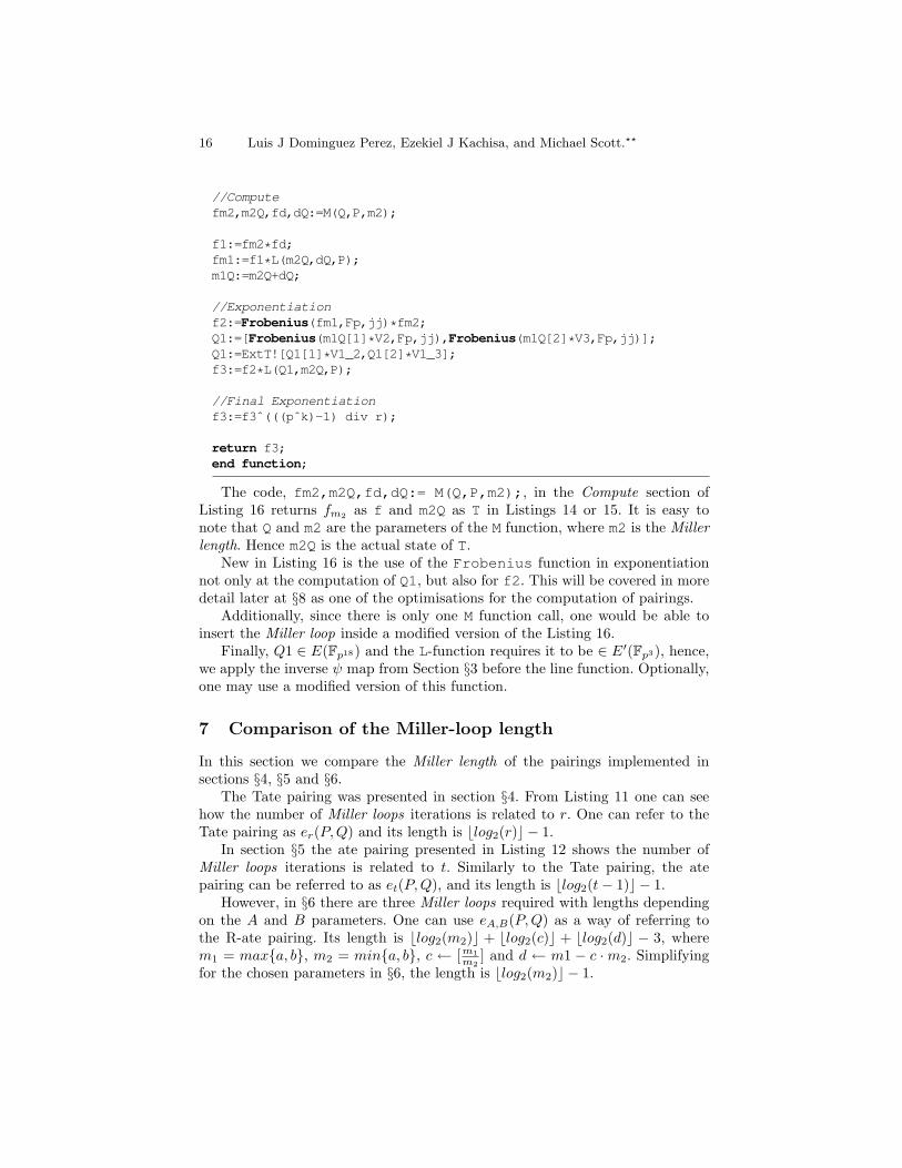
The code, fm2,m2Q,fd,dQ:= M(Q,P,m2);, in the Compute section ofListing 16 returns fm2 as f and m2Q as T in Listings 14 or 15. It is easy tonote that Q and m2 are the parameters of the M function, where m2 is the Millerlength. Hence m2Q is the actual state of T.
New in Listing 16 is the use of the Frobenius function in exponentiationnot only at the computation of Q1, but also for f2. This will be covered in moredetail later at §8 as one of the optimisations for the computation of pairings.
Additionally, since there is only one M function call, one would be able toinsert the Miller loop inside a modified version of the Listing 16.
Finally, Q1 ∈ E(Fp18) and the L-function requires it to be ∈ E′(Fp3), hence,we apply the inverse ψ map from Section §3 before the line function. Optionally,one may use a modified version of this function.
7 Comparison of the Miller-loop length
In this section we compare the Miller length of the pairings implemented insections §4, §5 and §6.
The Tate pairing was presented in section §4. From Listing 11 one can seehow the number of Miller loops iterations is related to r. One can refer to theTate pairing as er(P,Q) and its length is blog2(r)c − 1.
In section §5 the ate pairing presented in Listing 12 shows the number ofMiller loops iterations is related to t. Similarly to the Tate pairing, the atepairing can be referred to as et(P,Q), and its length is blog2(t− 1)c − 1.
However, in §6 there are three Miller loops required with lengths dependingon the A and B parameters. One can use eA,B(P,Q) as a way of referring tothe R-ate pairing. Its length is blog2(m2)c + blog2(c)c + blog2(d)c − 3, wherem1 = max{a, b}, m2 = min{a, b}, c ← [m1
m2] and d ← m1 − c ·m2. Simplifying
for the chosen parameters in §6, the length is blog2(m2)c − 1.
Implementing Cryptographic pairings: a magma tutorial 17
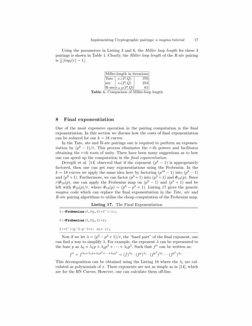
Using the parameters in Listing 3 and 6, the Miller loop length for these 3pairings is shown in Table 1. Clearly, the Miller loop length of the R-ate pairingis 1
One of the most expensive operation in the pairing computation is the finalexponentiation. In this section we discuss how the costs of final exponentiationcan be reduced for our k = 18 curves.
In the Tate, ate and R-ate pairings one is required to perform an exponen-tiation by (pk − 1)/r. This process eliminates the r-th powers and facilitatesobtaining the r-th roots of unity. There have been many suggestions as to howone can speed up the computation in the final exponentiation.
Devegili et al. [14] observed that if the exponent (pk − 1) is appropriatelyfactored, then one can get easy exponentiations using the Frobenius. In thek = 18 curves we apply the same idea here by factoring (p18 − 1) into (p9 − 1)and (p9 +1). Furthermore, we can factor (p9 +1) into (p3 +1) and Φ18(p). Sincer|Φ18(p), one can apply the Frobenius map on (p9 − 1) and (p3 + 1) and beleft with Φ18(p)/r, where Φ18(p) = (p6 − p3 + 1). Listing 17 gives the genericmagma code which can replace the final exponentiation in the Tate, ate andR-ate pairing algorithms to utilise the cheap computation of the Frobenius map.
Listing 17. The Final Exponentiation
f:=Frobenius(f,Fp,9)*fˆ(-1);
f:=Frobenius(f,Fp,3)*f;
f:=fˆ((pˆ6-pˆ3+1) div r);
Now if we let λ = (p6− p3 + 1)/r, the “hard part” of the final exponent, onecan find a way to simplify λ. For example, the exponent λ can be represented tothe base p as λ0 + λ1p+ λ2p
2 + · · ·+ λ5p5. Such that fλ can be written as:
fλ = fλ0+λ1p+λ2p2+···+λ5p5= (f)λ0 · (fp)λ1 · (fp2
)λ2 · · · (fp5)λ5
This decomposition can be obtained using the Listing 18 where the λi are cal-culated as polynomials of x. These exponents are not as simple as in [14], whichare for the BN Curves. However, one can calculate them off-line.
18 Luis J Dominguez Perez, Ezekiel J Kachisa, and Michael Scott.??
Listing 18. Base p representation of the λ exponent
1763*x + 2401) / 21;rx:=(xˆ6 + 37*xˆ3 + 343) div 343;lambda:= [];Append(˜lambda,(pxˆ6-pxˆ3+1) div rx);for i:=1 to 5 doAppend(˜lambda,lambda[i] mod pxˆ(6-i));
end for;for i:=1 to 6 dolambda[i]:= Evaluate(lambda[i] div pxˆ(6-i),xx);
end for;
return lambda;end function;
As before, one can use the Frobenius exponentiation for the fpi
elementscombined with any multi-exponentiation technique. However, we can use thesame approach as in [39, 7.2] to simplify the computation of the hard part of thefinal exponentiation.
Listing 19. Code for the hard part of the final exponentiation
During the computations some intermediate results are required and one canstill gain some advantages optimizing the code to use less memory.
It will be necessary to change the last line of §17 to f:=HardExpo(f,xx);in order to call this function. This will result in a significant gain in speed.
9 Multiplication in G2
Gallant, Lambert and Vanstone [19] introduced a method to speed up generalpoint multiplication nP ∈ E(Fp)[r] when there is an efficient computable en-domorphism ψ on E defined over Fp such that ψ(P ) = λP . In the case of thispaper, since KSS k = 18 curves [27] have the form y2 = x3 +b as in [19, Example4], the GLV method applies and it would require only one multiplication in Fp
to apply the endomorphism to point in G1.The idea is to compute nP efficiently by writing n ≡ n0+n1λ (mod r) with
|ni| <√r and performing a double exponentiation n0P + n1ψ(P ) [19]. In this
case, the number of bits in n0 and n1 are half the bitlength of n. One can savea significant number of point doublings at the expense of a few point additionsand the application of a map. If the map ψ is also cheaper than a point additionthen, it is possible to get a few extra computational savings.
Gallant et al [19] pointed that their method can be generalised for usinghigher powers of the endomorphism. Galbraith and Scott [22] recently showed atechnique on how to do it for the groups G2 and GT , as follows.
To get an m-dimensional expansion n ≡ n0+n1λ+. . .+nm−1λm−1 (mod r)
of nP , one must compose n with powers of λ sufficiently different modulo r.This can be done by solving a closest vector problem in a lattice as done in theBabai’s rounding method [2]. However, an LLL-reduced lattice basis must beprecomputed[22].
For KSS k = 18 curves [27], it will be possible to get a “natural” 6-dimensionalexpansion.
Implementing Cryptographic pairings: a magma tutorial 21
The modular lattice basis is defined as follows:
L =
{x ∈ Zm :
m−1∑i=0
xiλi ≡ 0 (mod r)
}
where λ = T = t − 1 as in [22, Example 5].This 6-dimensional modular latticeL will be used to construct a 6 × 6 matrix. Then, one can fill the matrix withany combination of λ that gives Li,j ≡ 0 (mod r). One can use a predefinedsequence of values for the L-matrix to be LLL-reduced, however it is possible touse random values. See Listing 20 for a random and an ordered definition of thematrix L. Also see the function LLL() for the LLL-reduction at the end of theprogram.
Listing 20. Initial Lattice and LLL-reduction
x:=25672080793808285942;m:=6;r:=(xˆ6 + 37*xˆ3 + 343) div 343;t:=(xˆ4+16*x)/7+1;lambda:=t-1;
// Option 1, randomlyL:= Matrix(Rationals(), m, [lambda,-1,0,0,lambda,-1,0,0,lambda,-1,0,0,0,0,0,lambda,-1,0,0,lambda,-1,0,lambda,-1,lambda,-1,0,lambda,-1,0,r,lambda,-1,lambda,-1,0
]);
// Option 2, orderedL:= Matrix(Rationals(), m, [r,0,0,0,0,0,lambda,-1,0,0,0,0,lambdaˆ2,0,-1,0,0,0,lambdaˆ3,0,0,-1,0,0,lambdaˆ4,0,0,0,-1,0,lambdaˆ5,0,0,0,0,-1
]);
B:=LLL(L);
This way, B is the LLL-reduced matrix, similarly to [22, Example 5]. Notethat one can automate the L creation in the second matrix in Listing 20.
One can verify the lattice consistency mod r with the code in Listing 21
Listing 21. Validate matrix B
checklattice:=procedure(L)sum:=0;
22 Luis J Dominguez Perez, Ezekiel J Kachisa, and Michael Scott.??
for i:=1 to m dofor j:= 1 to m dosum:=sum+L[i][j]*lambdaˆ(j-1);
end for;sum:= Integers()!sum mod r;if sum eq 0 then print "OK"; else print "BAD",i; end if;sum:=0;
end for;end procedure;
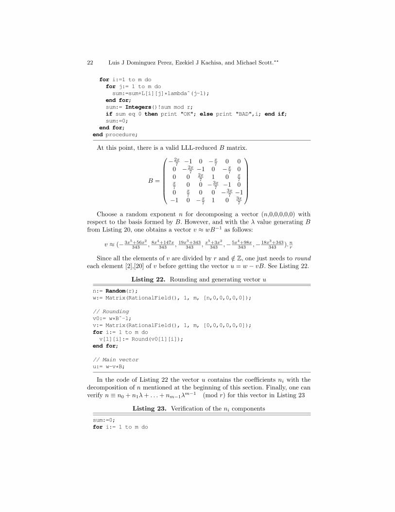
At this point, there is a valid LLL-reduced B matrix.
B =
− 2x
7 −1 0 −x7 0 0
0 − 2x7 −1 0 −x
7 00 0 2x
7 1 0 x7
x7 0 0 − 3x
7 −1 00 x
7 0 0 − 3x7 −1
−1 0 −x7 1 0 3x
7
Choose a random exponent n for decomposing a vector (n,0,0,0,0,0) with
respect to the basis formed by B. However, and with the λ value generating Bfrom Listing 20, one obtains a vector v ≈ wB−1 as follows:
v ≈ (− 3x5+56x2
343 , 8x4+147x343 , 19x3+343
343 , x5+3x2
343 ,− 5x4+98x343 ,− 18x3+343
343 ).nr
Since all the elements of v are divided by r and /∈ Z, one just needs to roundeach element [2],[20] of v before getting the vector u = w − vB. See Listing 22.
Listing 22. Rounding and generating vector u
n:= Random(r);w:= Matrix(RationalField(), 1, m, [n,0,0,0,0,0]);
// Roundingv0:= w*Bˆ-1;v:= Matrix(RationalField(), 1, m, [0,0,0,0,0,0]);for i:= 1 to m dov[1][i]:= Round(v0[1][i]);
end for;
// Main vectoru:= w-v*B;
In the code of Listing 22 the vector u contains the coefficients ni with thedecomposition of n mentioned at the beginning of this section. Finally, one canverify n ≡ n0 + n1λ+ . . .+ nm−1λ
m−1 (mod r) for this vector in Listing 23
Listing 23. Verification of the ni components
sum:=0;for i:= 1 to m do
Implementing Cryptographic pairings: a magma tutorial 23
sum:= sum + u[1][i]*lambdaˆ(i-1);end for;if (Integers()!sum mod r) eq n then print "OK" else print "BAD";
10 Conclusion
In this paper we have taken the reader through the processes of implementationof pairings on a pairing-friendly elliptic curves using the magma software. Thishas been demonstrated using a family of pairing friendly elliptic curves of em-bedding degree 18. Some optimizations such as the use of a twist of a curve andmethods to speed up the final exponentiation have been discussed in relation tok = 18 curves. These optimisations can be extended to other embedding degreeswith similar structure. The code in this paper can be used as a basic guide inthe implementation of cryptographic pairings.
11 Acknowledgements
The authors would like to thank Professor Gary McGuire UCD(CSI) for hisuseful clarifications on the counting of points on the elliptic curves.
References
1. Antonio, C.A., Tanaka, S. and Nakamula, K., (2007) Implementing CryptographicPairings over Curves of Embedding Degrees 8 and 10. Cryptology ePrint ArchiveReport 2007/426, http://eprint.iacr.org/2007/426.
2. Babai, Li. (1986) On Lovasz lattice reduction and the nearest lattice point problem.Combinatronica 1986, 6(1), pp. 1–13, Springer-Verlag.
3. Barreto P.S.L.M., Lynn, B., Kim H. and Scott, M. (2002) Efficient Algorithmsfor Pairing-Based Cryptosystems. Advances in Cryptology – Crypto’2002, LectureNotes in Computer Science 2442, pp. 354-368, Springer-Verlag
4. Barreto P.S.L.M., Lynn, B. and Scott, M., (2002) Constructing elliptic curves withprescribed embedding degree. Security in Communication Networks -SCN 2002, Lec-ture Notes in Computer Science 2576, pp. 263–273, Springer-Verlag
5. Barreto P.S.L.M., Lynn, B. and Scott, M., (2003) On the Selection of Pairing-Friendly Groups. Symposium on Applied Computing -SAC 2003, Lecture Notes inComputer Science 3006, pp. 17–25, Springer-Verlag
6. Barreto, P.S.L.M., and Naehrig M., (2006) Pairing-friendly elliptic curves of primeorder. Selected Areas in Cryptography – SAC’2005, Lecture Notes in ComputerScience 3897, pp 319–331 Springer-Verlag
7. Blake, I., Seroussi, G., and Smart, N., (1994) Elliptic Curves in Cryptography.London Mathematical Society, Cambridge: Cambridge University Press.
8. Blake, I., Seroussi, G., and Smart, N. (2005). Advances in Elliptic Curve Cryptog-raphy. Cambridge University Press.
9. Boneh, D., Franklin, M. (2001) Identity-based encryption from the Weil pairing.Lecture Notes in Computer Science 2139, pp. 213229, Springer-Verlag.
24 Luis J Dominguez Perez, Ezekiel J Kachisa, and Michael Scott.??
10. Boneh, D., Lynn, B., and Shacham, H. (2001). Short Signatures from the WeilPairing. Lecture Notes in Computer Science 2248, pp. 514-532. Springer, Verlag.
11. Bosma, W., Cannon, J., and Playoust, C. (1997). The Magma algebra system. I.The user language. J. Symbolic Comput., 24(3-4):235-265, 1997
12. Brezing F. and Weng A., (2005) Elliptic curves suitable for pairing based cryptog-raphy., Designs Codes and Cryptography, Vol. 37, No. 1, pp. 133–141
13. Cohen, H., Frey, G. (2006). Hanbook of Elliptic and Hyperelliptic Curve Cryptog-raphy Chapman & Hall/CRC
14. Devegili, A. J., Scott, M. and Dahab R., (2007) Implementing Cryptographic Pair-ings over Barreto-Naehrig Curves. Pairing 2007, Lecture Notes in Computer Sci-ence 4575, pp. 197–207, Springer-Verlag
15. Freeman, D., (2006) Constructing pairing-friendly elliptic curves with embeddingDegree 10. In Algorithmic Number Theory Symposium ANTS-VII, Lecture Notesin Computer Science 4096, pp. 452–465. Springer-Verlag
16. Freeman, D., Scott, M. and Teske, E., (2006) A Taxonomy of pairing-fri-endly elliptic curves. Cryptography ePrint Archive, Report 2006/372, http://eprint.iacr.org/2006/372
17. Frey, G. (2001). Applications of Arithmetical Geometry to Cryptographic Construc-tions Finite Field 5, 128–161, 2001.
18. Frey, G., and Ruck, H-G., (1994). A Remark concerning m-Divisibility and theDiscrete Logarithm in the Divisor Class Group of Curves. Mathematics of Com-putation, Volume 62, Number 206, pp. 865–874. American Mathematical Society.
19. Gallant Robert P., Lambert, Robert J., and Vanstone, Scott A. Faster Point Mul-tiplication on Elliptic Curves with Efficient Endomorphisms. Crypto 2001, LectureNotes in Computer Science 2139, pp 190–200. Springer-Verlag.
20. Galbraith, S.D. Personal communication.21. Galbraith, S.D, McKee, J. and Valenca, P., (2004) Ordinary Abelian varieties
having small embedding degree. Cryptography ePrint Archive, Report 2004/365,http://eprint.iacr.org/2004/365.
22. Galbraith, S. D., Scott, M. (2008). Exponentiation in pairing-friendly groups usinghomomorphisms. Pairing 2008, Lecture Notes in Computer Science 5209, pp 211–224 Springer-Verlag
23. Hankerson, D., Menezes, A. and Vanstone, S., (2004) Guide to elliptic curve cryp-tography. New York: Springer-Verlag.
24. Hess, F., Smart, N. and Vercauteren F., (2006) The Eta Pairing revisited. IEEETrans. Information Theory, Vol. 52, pp. 4595–4602
25. IEEE Standard Specification 1363-2000. Annex A. IEEE, 2000.26. Joux, A, (2000). A One Round Protocol for Tripartite DiffieHellman. Lecture Notes
in Computer Science, 1838, pp. 385-394. Springer, Verlag.27. Kachisa, E., Schaeffer, E.F. and Scott M (2007) Constructing Brezing-Weng pairing
friendly elliptic curves using elements in the cyclotomic field, Pairing 2008, LectureNotes in Computer Science 5209, pp 126–135 Springer-Verlag
28. Koblitz, N., Menezes, A. Pairing-Based Cryptography at High Security Levels Lec-ture Notes in Computer Science 3796, pp 13–36, 2005.
29. Lee, E., Lee, H.-S., Park,C.-M. Efficient and Generalized Pairing Computation onAbelian Varieties Cryptology ePrint Archive, Report 2008/040, 2008.
30. Lenstra, A. K. Unbelievable Security Matching AES security using public key sys-tems, http://www.win.tue.nl/ klenstra/aes match.pdf
31. Matsuda, S., Kanayama, N., Hess, F. and Okamoto, E., (2007) Optimised versionsof the ate and Twisted ate Pairings. Cryptology ePrint Archive, Report 2007/013,http://eprint.iacr.org/2007/013
Implementing Cryptographic pairings: a magma tutorial 25
32. Menezes, A., Okamoto, T., and Vanstone, S., (1991) Reducing Elliptic Curve Log-arithms to Logarithms in a Finite Field. Proceedings of the twenty-third annualACM symposium on Theory of computing, pp. 80-89. Association for ComputingMachinery.
33. Miller, V. S. Short Programs for functions on Curves. IBM Thomas J. WatsonResearch Center (available at http://crypto.stanford.edu/Miller/Miller.ps), 1986.
34. Mitsunari, A., Sakai, R., and Kasahara, M. (2002). A New Traitor Tracing. Trans-actions on Fundamentals of Electronics, Communications and Computer Science,vol. E85-A, no. 2, pp. 481-484.
35. Miyaji, A., Nakabayashi, M. and Takano, S., (2001) New explicit conditions ofelliptic curve traces for FR-reduction. IEICE Trans. Fundamentals, E84 pp. 1234- 1243.
36. Naehrig, M. and Barreto, P.S.L.M., (2007) On compressible pairings and theircomputation. Progress in Cryptology AFRICACRYPT 2008. Lecture Notes inComputer Science, 5023, pp 371-388. Springer-Verlag
37. Sakai, R., Ohgishi, K., and Kasahara, M. (2000). Cryptosystems based on pair-ing. Symposium on Cryptography and Information Security (SCIS2000), Okinawa,Japan, Jan. 2628, 2000.
38. Scott, M. (2007). Implementing Cryptographic Pairings. Lecture Notes in Com-puter Science, 4575, pp. 177–196. Springer, Verlag.
39. Scott, M. Benger, N. Charlemagne, M. Dominguez P., L. J., Kachiza, E. (2008).On the final exponentiation for calculating pairings on ordinary elliptic curves.Cryptology ePrint Archive, Report 2008/490, http://eprint.iacr.org/2008/490
40. Scott, M. Benger, N. Charlemagne, M. Dominguez P., L. J., Kachiza, E. (2008).Fast hashing to G2 on pairing friendly curves. Cryptology ePrint Archive, Report2008/530, http://eprint.iacr.org/2008/530
41. Shamir, A. (1984). Identity-Based Cryptosystems and Signature Schemes. LectureNotes in Computer Science, 196, pp. 47-53. Springer, Verlag.
42. Silverman, J. H. (1986). The Arithmetic of Elliptic Curves. Springer-Verlag.
43. Solinas, J. A. (2003). ID-Based Digital Signature Algorithms. ECC 2003. http://www.cacr.math.uwaterloo.ca/conferences/2003/ecc2003/solinas.pdf
44. Tanaka, S. and Nakamula, K., (2007) More constructing pairing-friendly el-liptic curves for cryptography. Mathematics arXiv Archive, Report 0711.1942,http://arxiv.org/abs/0711.1942
45. Zhao, C-A., and Zhang, F. and Huang, J., (2007) A Note on the ate Pairing.Cryptology ePrint Archive, Report 2007/247, http://eprint.iacr.org/2007/247
Appendix
A Counting rational points on the curve
The number of points on an elliptic curve is related to the size of the field asfollows #E(Fp) = p + 1 − t, where t is the trace of the Frobenious of Endor-morphism. If α is a root to the characteristic polynomial X2 − tX + p, thenthe number of points on the curve defined over the extension field is defined asfollows, #E(Fpk) = pk + 1 − αk − αk. In magma one compute the number ofpoints on E(Fpk) using the following code:
26 Luis J Dominguez Perez, Ezekiel J Kachisa, and Michael Scott.??
Listing 24. Counting points in the curve over the extension field
// Input <- (p,k,t) defining the Elliptic Curve// Output -> The number of points in the curveGetnpFpk:= function(p,k,t)tr:=[];Append(˜tr,2);Append(˜tr,t);for i:=2 to k doAppend(˜tr,t*tr[i]-p*tr[i-1]);
end for;return (pˆk)+1-tr[k+1];end function;
However, when constructing a twist curve the number of rational pointsvaries. For k = 18, for example, one can define q = p3 and T = t3 − 3pt fora sextic twist of these curves [24]. Then, #E′(Fq) = q + 1 − (3F + T )/2, withT 2− 4q = −3F 2. Solving for F , one can easily calculate the number of points inthe twisted curve as in Listing 25.
Listing 25. Counting points in the curve over the twisted curve
// Input <- (p,k,t) defining the Elliptic Curve// Output -> The number of rational points on the twisted curve
over Fpˆ3GetnpFp3:= function(p,k,t)q:=pˆ3;T:=tˆ3-3*p*t;F:=Isqrt((Tˆ2-4*q) div -3);np:=q+1-(3*F+T) div 2;
return np;end function;
B Ti selection
The authors used a previously calculated Ti-Tj combination of 37x.T6 + 2
7x. Inthis section is presented a way to get all the valid combinations.
It has been stated that Ti ≡ pimod r and A = a.B + b. Then, Ti = a.Tj + b,similary Tj ≡ pj mod r. However, it is also possible to use (t− 1)imod r.
One can calculate all the Ti-Tj combinations and compare later. First, it isnecessary to generate all the Ti’s. There are up to k possible polynomials. Oneway to obtain them is shown as Listing 26.
Implementing Cryptographic pairings: a magma tutorial 27
rx:=(xˆ6 + 37*xˆ3 + 343) div 343;
Poly:=[];for i:=0 to k-1 do
Append(˜Poly,(pxˆi) mod rx);end for;
In Listing 26 RationalField is being used for defining the p(x) and r(x)polynomials from [27]. One can modify these polynomials, with its respectivek to calculate to corresponding Ti’s polynomials for a different elliptic curvefamily.
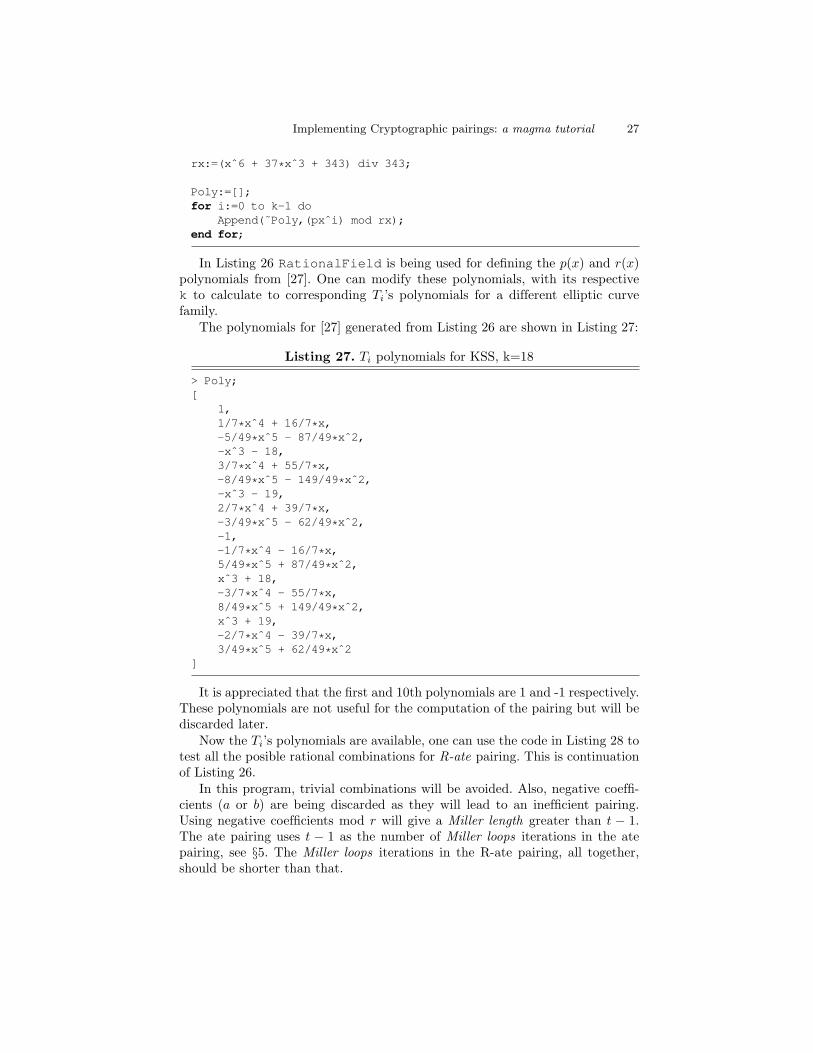
The polynomials for [27] generated from Listing 26 are shown in Listing 27:
It is appreciated that the first and 10th polynomials are 1 and -1 respectively.These polynomials are not useful for the computation of the pairing but will bediscarded later.
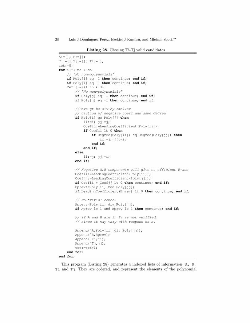
Now the Ti’s polynomials are available, one can use the code in Listing 28 totest all the posible rational combinations for R-ate pairing. This is continuationof Listing 26.
In this program, trivial combinations will be avoided. Also, negative coeffi-cients (a or b) are being discarded as they will lead to an inefficient pairing.Using negative coefficients mod r will give a Miller length greater than t − 1.The ate pairing uses t − 1 as the number of Miller loops iterations in the atepairing, see §5. The Miller loops iterations in the R-ate pairing, all together,should be shorter than that.
28 Luis J Dominguez Perez, Ezekiel J Kachisa, and Michael Scott.??
Listing 28. Chosing Ti-Tj valid candidates
A:=[]; B:=[];Ti:=[];Tj:=[]; Tl:=[];tot:=0;for i:=1 to k do
// "No non-polynomials"if Poly[i] eq 1 then continue; end if;if Poly[i] eq -1 then continue; end if;for j:=i+1 to k do
// "No non-polynomials"if Poly[j] eq 1 then continue; end if;if Poly[j] eq -1 then continue; end if;
//Have gt be div by smaller// caution w/ negative coeff and same degreeif Poly[i] ge Poly[j] then
ii:=i; jj:=j;Coefii:=LeadingCoefficient(Poly[ii]);if Coefii lt 0 then
if Degree(Poly[ii]) eq Degree(Poly[jj]) thenii:=j; jj:=i;
end if;end if;
elseii:=j; jj:=i;
end if;
// Negative A,B components will give no efficient R-ateCoefii:=LeadingCoefficient(Poly[ii]);Coefjj:=LeadingCoefficient(Poly[jj]);if Coefii * Coefjj lt 0 then continue; end if;Bprev:=Poly[ii] mod Poly[jj];if LeadingCoefficient(Bprev) lt 0 then continue; end if;
// No trivial combo.Aprev:=Poly[ii] div Poly[jj];if Aprev le 1 and Bprev le 1 then continue; end if;
// if A and B are in Zz is not verified,// since it may vary with respect to x.
Append(˜A,Poly[ii] div Poly[jj]);Append(˜B,Bprev);Append(˜Ti,ii);Append(˜Tj,jj);tot:=tot+1;
end for;end for;
This program (Listing 28) generates 4 indexed lists of information: A, B,Ti and Tj. They are ordered, and represent the elements of the polynomial
Implementing Cryptographic pairings: a magma tutorial 29
A = a.B + b in the following way: Ti = A.Tj + B (after substracting 1 fromTi and Tj). These combinations are the only candidates that are non-negative,non-trivial, and depending on its coefficients and the value of x can be ∈ Z.
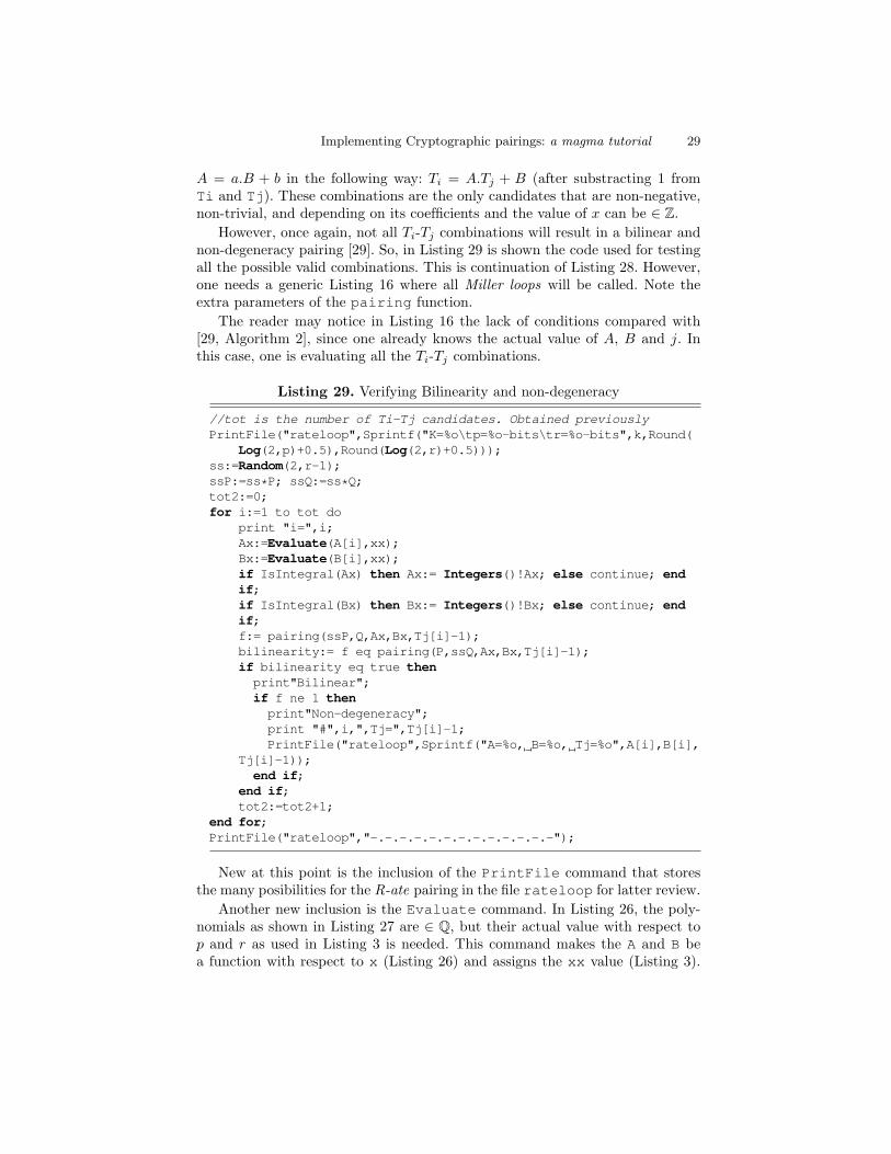
However, once again, not all Ti-Tj combinations will result in a bilinear andnon-degeneracy pairing [29]. So, in Listing 29 is shown the code used for testingall the possible valid combinations. This is continuation of Listing 28. However,one needs a generic Listing 16 where all Miller loops will be called. Note theextra parameters of the pairing function.
The reader may notice in Listing 16 the lack of conditions compared with[29, Algorithm 2], since one already knows the actual value of A, B and j. Inthis case, one is evaluating all the Ti-Tj combinations.
Listing 29. Verifying Bilinearity and non-degeneracy
//tot is the number of Ti-Tj candidates. Obtained previouslyPrintFile("rateloop",Sprintf("K=%o\tp=%o-bits\tr=%o-bits",k,Round(
Log(2,p)+0.5),Round(Log(2,r)+0.5)));ss:=Random(2,r-1);ssP:=ss*P; ssQ:=ss*Q;tot2:=0;for i:=1 to tot do
print "i=",i;Ax:=Evaluate(A[i],xx);Bx:=Evaluate(B[i],xx);if IsIntegral(Ax) then Ax:= Integers()!Ax; else continue; endif;if IsIntegral(Bx) then Bx:= Integers()!Bx; else continue; endif;f:= pairing(ssP,Q,Ax,Bx,Tj[i]-1);bilinearity:= f eq pairing(P,ssQ,Ax,Bx,Tj[i]-1);if bilinearity eq true thenprint"Bilinear";if f ne 1 thenprint"Non-degeneracy";print "#",i,",Tj=",Tj[i]-1;PrintFile("rateloop",Sprintf("A=%o, B=%o, Tj=%o",A[i],B[i],
Tj[i]-1));end if;
end if;tot2:=tot2+1;
end for;PrintFile("rateloop","-.-.-.-.-.-.-.-.-.-.-.-.-");
New at this point is the inclusion of the PrintFile command that storesthe many posibilities for the R-ate pairing in the file rateloop for latter review.
Another new inclusion is the Evaluate command. In Listing 26, the poly-nomials as shown in Listing 27 are ∈ Q, but their actual value with respect top and r as used in Listing 3 is needed. This command makes the A and B bea function with respect to x (Listing 26) and assigns the xx value (Listing 3).
30 Luis J Dominguez Perez, Ezekiel J Kachisa, and Michael Scott.??
Since they are used as execution times, one needs to verify if these evaluates∈ N. Otherwise, such combination should be discarded.
For the evaluation of the bilinearity, one creates ss a Random number andcreates ssP and ssQ as ss*P and ss*Q with P and Q respectively as fromListing 3. And they are used for verifying the bilinearity: e(P, ssQ) = e(ssP,Q).Also the non-degeneracy property is evaluated: e(P,Q) 6= 1.
The reader must load additionally to the Listing 3 and 14, the modifiedListing 16 for computing the pairing. Listing 8 for the points definition. AndListing 26, 28 and, 29 for the generation of the Ti-Tj combinations.
Once the Ti-Tj combinations are generated. The reader must choose theshortest one from the generated rateloop file from Listing 29. Some readersmay prefer another combination, and make its own optimizations. For examplethe 11th combination from the rateloop file: 2
7xT12 + 37x combination is quite
similar, but is left to the reader as an exercise.