Improved Lesion Detection UsingNonlocal Means Post-Processing

Ole Marius Hoel Rindal∗, Alfonso Rodriguez-Molares∗†‡, Svein-Erik Masøy†‡ and Tore Gruner Bjastad†‡

∗Department of InformaticsUniversity of Oslo

Oslo, NorwayEmail: omrindal@ifi.uio.no

†Department of Circulation andMedical Imaging

Norwegian University of Science andTechnology

Trondheim, Norway

‡InPhase Solutions ASTrondheim, Norway

Abstract—Software beamforming allows more flexible andcomplex algorithms, often referred to as adaptive beamformingtechniques, that are blurring the boundaries between beam-forming and image processing. Many adaptive beamformingalgorithms claim to improve lesion detectability. Based on recentadvances, we hypothesize that image processing techniques thatreduce speckle variability yield better lesion detectability thanstate-of-the-art adaptive beamformers.

This hypothesis is investigated on six algorithms: two imageprocessing techniques, and four adaptive beamformers. As atarget we use Field II simulations of a hypoechoic cyst withnoise added to simulate different SNR conditions. Lesion de-tectability is estimated using the Generalized Contrast-to-NoiseRatio (GCNR). The results support our hypothesis.

Index Terms—Lesion detection, adaptive beamforming, coher-ence beamforming, Generalized Contrast-to-Noise Ratio.

I. INTRODUCTION

Lesion detectability of an imaging method has traditionallybeen estimated using either the contrast ratio (CR) or thecontrast-to-noise ratio (CNR). It has recently been shown thatCR and CNR can be arbitrarily increased by dynamic rangetransformations [1]. A new metric has been introduced, thegeneralized-contrast-to-noise ratio (GCNR) [2], which esti-mates the maximum classification rate that can be achievedby an optimal observer.

detected not detectedε = ε0

pi(x)

po(x)

PF PM

x

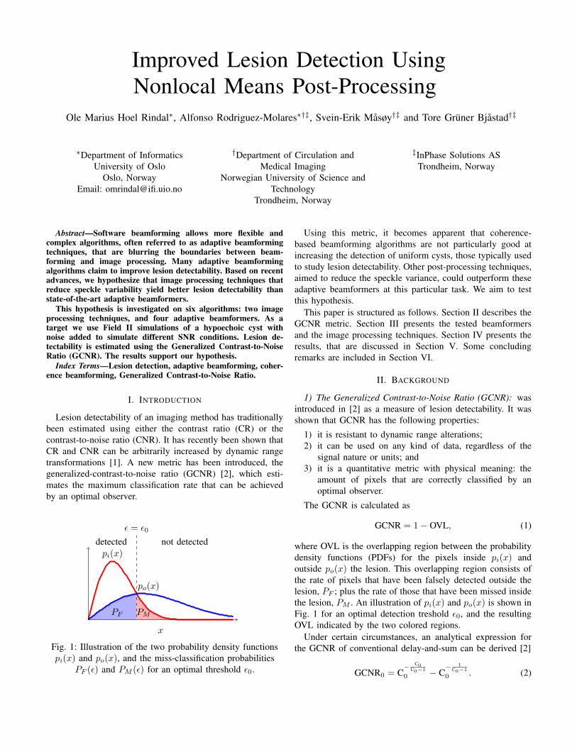
Fig. 1: Illustration of the two probability density functionspi(x) and po(x), and the miss-classification probabilities

PF (ε) and PM (ε) for an optimal threshold ε0.

Using this metric, it becomes apparent that coherence-based beamforming algorithms are not particularly good atincreasing the detection of uniform cysts, those typically usedto study lesion detectability. Other post-processing techniques,aimed to reduce the speckle variance, could outperform theseadaptive beamformers at this particular task. We aim to testthis hypothesis.

This paper is structured as follows. Section II describes theGCNR metric. Section III presents the tested beamformersand the image processing techniques. Section IV presents theresults, that are discussed in Section V. Some concludingremarks are included in Section VI.

II. BACKGROUND

1) The Generalized Contrast-to-Noise Ratio (GCNR): wasintroduced in [2] as a measure of lesion detectability. It wasshown that GCNR has the following properties:

1) it is resistant to dynamic range alterations;2) it can be used on any kind of data, regardless of the

signal nature or units; and3) it is a quantitative metric with physical meaning: the

amount of pixels that are correctly classified by anoptimal observer.

The GCNR is calculated as

GCNR = 1− OVL, (1)

where OVL is the overlapping region between the probabilitydensity functions (PDFs) for the pixels inside pi(x) andoutside po(x) the lesion. This overlapping region consists ofthe rate of pixels that have been falsely detected outside thelesion, PF ; plus the rate of those that have been missed insidethe lesion, PM . An illustration of pi(x) and po(x) is shown inFig. 1 for an optimal detection treshold ε0, and the resultingOVL indicated by the two colored regions.

Under certain circumstances, an analytical expression forthe GCNR of conventional delay-and-sum can be derived [2]

GCNR0 = C− C0

C0−1

0 − C− 1

C0−1

0 . (2)

where C0 can be calculated dependant on the number ofelements M and the channel SNR

C0 =3

2M SNR + 3. (3)

III. METHODS

We used Field II [3][4] to simulate a 6 mm diameteranechoic cyst using a synthetic transmit aperture sequence anda 128-element, 300 um, linear probe transmitting at 5.13 MHz.A total of 20 datasets were generated. Band-pass Gaussiannoise was added with different intensities to simulate channelSNR conditions from -20.7 to 4.4 dB.

The datasets were processed using 6 image formation meth-ods:

1) delay-and-sum and spatial averaging (DAS + SA), usinga 2D kernel of 30 pixels;

2) delay-and-sum and nonlocal means [5] (DAS + NLM),with parameters resulting in a search radi and compar-ison radi of 30 by 30 pixels, a preselection thresholdof 4, σ = 80 assuming a Gaussian distribution of thepixels;

3) phase coherence factor (PCF) [6], with γ = 1;4) generalized coherence factor (GCF) [7], with M0=4;5) short lag spatial coherence (SLSC-λ) [8], with Mmax =

14 and a λ kernel size; and6) short lag spatial coherence (SLSC-0.1λ) [8], with

Mmax = 14 and a 0.1λ kernel size.Both spatial averaging and nonlocal means was applied after

envelope detection and logarithmic compression. GCNR wasestimated using Eq. (1) for all SNR conditions. Fig. 4a showsthe regions i, red, and o, blue, used to calculate GCNR.

All processing was done in MATLAB (The MathWorks,Natick, USA) using the UltraSound ToolBox (USTB) [9]. Thedata and code needed to produce all figures and results areavailable at http://www.ustb.no.

IV. RESULTS

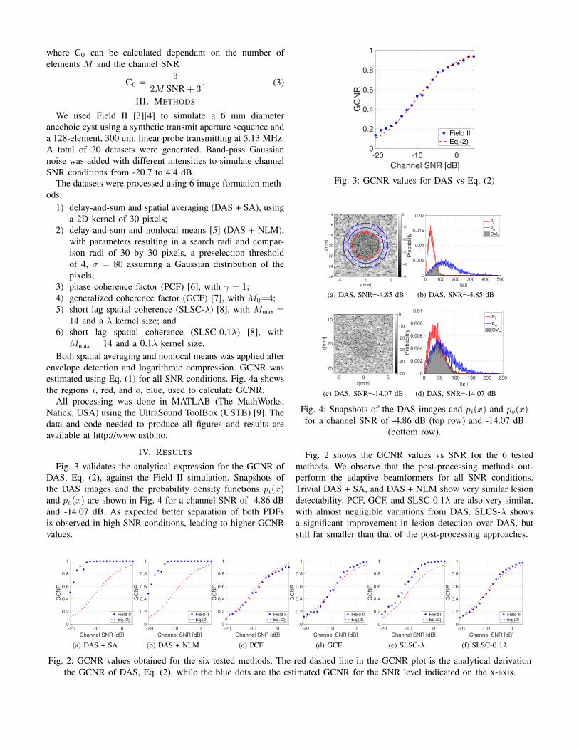
Fig. 3 validates the analytical expression for the GCNR ofDAS, Eq. (2), against the Field II simulation. Snapshots ofthe DAS images and the probability density functions pi(x)and po(x) are shown in Fig. 4 for a channel SNR of -4.86 dBand -14.07 dB. As expected better separation of both PDFsis observed in high SNR conditions, leading to higher GCNRvalues.

-20 -10 0

Channel SNR [dB]

0

0.2

0.4

0.6

0.8

1

GC

NR

Field II

Eq.(2)

Fig. 3: GCNR values for DAS vs Eq. (2)

-5 0 5

x[mm]

14

16

18

20

22

24

26

z[m

m]

-50

-40

-30

-20

-10

0

(a) DAS, SNR=-4.85 dB

0 100 200 300 400 500

||s||

0

0.005

0.01

0.015

0.02

Pro

ba

bili

ty

pi

po

OVL

(b) DAS, SNR=-4.85 dB

-5 0 5

x[mm]

15

20

25

z[m

m]

-50

-40

-30

-20

-10

0

(c) DAS, SNR=-14.07 dB

0 50 100 150 200 250

||s||

0

0.002

0.004

0.006

0.008

0.01

Pro

ba

bili

ty

pi

po

OVL

(d) DAS, SNR=-14.07 dB

Fig. 4: Snapshots of the DAS images and pi(x) and po(x)for a channel SNR of -4.86 dB (top row) and -14.07 dB

(bottom row).

Fig. 2 shows the GCNR values vs SNR for the 6 testedmethods. We observe that the post-processing methods out-perform the adaptive beamformers for all SNR conditions.Trivial DAS + SA, and DAS + NLM show very similar lesiondetectability. PCF, GCF, and SLSC-0.1λ are also very similar,with almost negligible variations from DAS. SLCS-λ showsa significant improvement in lesion detection over DAS, butstill far smaller than that of the post-processing approaches.

-20 -10 0

Channel SNR [dB]

0

0.2

0.4

0.6

0.8

1

GC

NR

Field II

Eq.(2)

(a) DAS + SA

-20 -10 0

Channel SNR [dB]

0

0.2

0.4

0.6

0.8

1

GC

NR

Field II

Eq.(2)

(b) DAS + NLM

-20 -10 0

Channel SNR [dB]

0

0.2

0.4

0.6

0.8

1

GC

NR

Field II

Eq.(2)

(c) PCF

-20 -10 0

Channel SNR [dB]

0

0.2

0.4

0.6

0.8

1

GC

NR

Field II

Eq.(2)

(d) GCF

-20 -10 0

Channel SNR [dB]

0

0.2

0.4

0.6

0.8

1

GC

NR

Field II

Eq.(2)

(e) SLSC-λ

-20 -10 0

Channel SNR [dB]

0

0.2

0.4

0.6

0.8

1

GC

NR

Field II

Eq.(2)

(f) SLSC-0.1λ

Fig. 2: GCNR values obtained for the six tested methods. The red dashed line in the GCNR plot is the analytical derivationthe GCNR of DAS, Eq. (2), while the blue dots are the estimated GCNR for the SNR level indicated on the x-axis.

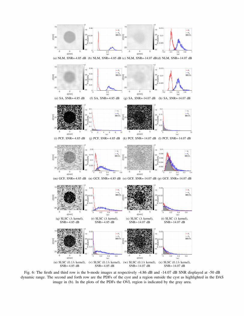
For completeness, we include in Fig. 6 the snapshots of theresulting images and probability density functions pi(x) andpo(x) for a channel SNR of -4.86 dB and -14.07 dB.

V. DISCUSSION

Our results show that DAS + SA and DAS + NLM providebetter lesion detectability than the tested coherence methods.This makes good sense: these averaging techniques reducespeckle variance both within and outside the lesion and makethe separation of both regions easier. This is confirmed bythe plots in Fig. 6, where we observe that, both, DAS + SAand DAS + NLM, reduce the variance of pi and po whileincreasing the distance between their means.

High lesion detectability can be achieved by trivial spatialaveraging (i.e. DAS + SA), however DAS + NLM does a betterjob at preserving the image resolution. Fig. 5 shows the lateralprofile through the center of the lesion at a channel SNR of4.35 dB. The edge of the cyst is sharper for the DAS + NLMalgorithm. This illustrates that lesion detectability alone is notenough to ascertain the superiority of any imaging algorithm;as one can, trivially, trade off lesion detectability againstspatial resolution. Lesion detectability should, therefore, beaccompanied by an evaluation of the corresponding spatialresolution.

-6 -4 -2 0 2 4 6

x [mm]

-30

-20

-10

0

Am

plit

ud

e [

dB

]

NLM

SA

Cyst edges

Fig. 5: Lateral profile through the center of the lesion forSNR = 4.35 dB for DAS + NLM and DAS + SA. Lesion

edges are indicated with dashed lines.

The results seem to indicate that coherence-based beam-formers are not particularly well-suited for the task of detect-ing purely scattering lesions. Perhaps they can be better usedto detect highly coherent targets, such as microcalcifications,or interfaces. Coherence beamforming has also been shown tobe able to aid in the differentiation between solid and fluid-filled masses in-vivo [10].

The effect of the user settable parameters was brieflyinvestigated. The SLSC implementation with a smaller kernelsize 0.1λ, Fig. 6u to 6x, led to lower GCNR values, Fig. 2f,than those obtained with larger kernel size λ, Fig. 6q to 6twith the resulting GCNR in Fig. 2e. This may indicate thatthe GCNR improvement observed in SLSC may be due to thisintroduced spatial averaging.

Our results demonstrate that the entire signal processingchain in ultrasound imaging is responsible for the final perfor-mance. However, a full implementation of the entire chainis a demanding task for an individual researcher. Havingan open source implementation of that chain, from channeldata to post-processing of the image, such as the USTB

(http://www.ustb.no), enable researchers to easily share theirresults and benefit from the others’ implementations. Webelieve this can help increasing the quality and efficiency ofthe research done by the ultrasound community.

Lastly, it is important to point out that the implementationsused here are not necessarily optimal for the detection ofscattering targets. Other implementations, better tuned for thedetection of particular lesion types, are of course possible.As an example, a real-time implementation of nonlocal-meansin [11] demonstrated impressive results in despeckling ofultrasound images.

VI. CONCLUSION

Post-processing of conventional delay-and-sum images us-ing trivial spatial averaging and a edge-preserving nonlocalmeans, outperforms state of the art coherence beamformingmethods at detecting scattering lesions. The methods’ lesiondetectability was evaluated using the Generalized Contrast-to-Noise Ratio (GCNR), a metric that measures the maximumclassification rate that can be achieved by an optimal observer.These results indicate that coherence-based beamformers arenot particularly well-suited for the task of detecting purelyscattering lesions.

REFERENCES

[1] O. M. H. Rindal, A. Austeng, A. Fatemi, and A. Rodriguez-Molares,“The Effect of Dynamic Range Alterations in the Estimation of Con-trast,” IEEE Transactions on Ultrasonics, Ferroelectrics, and FrequencyControl, vol. 66, no. 7, pp. 1198–1208, 2019.

[2] A. Rodriguez-Molares, O. M. H. Rindal, J. D’hooge, S.-E. Masøy,A. Austeng, and H. Torp, “The Generalized Contrast-to-Noise Ratio,”IEEE International Ultrasonics Symposium, IUS, no. 6, pp. 1–4, 2018.

[3] J. A. Jensen and N. B. Svendsen, “Calculation of Pressure Fields fromArbitrarily Shaped, Apodized, and Excited Ultrasound Transducers,”IEEE Transactions on Ultrasonics, Ferroelectrics and Frequency Con-trol, vol. 39, no. 2, pp. 262–267, 1992.

[4] J. A. Jensen, “Field: A program for simulating ultrasound systems,”Medical & Biological Engineering & Computing, vol. 34, pp. 351–353,1996.

[5] A. Tristan-Vega, V. Garcıa-Perez, S. Aja-Fernandez, and C. F. Westin,“Efficient and robust nonlocal means denoising of MR data basedon salient features matching,” Computer Methods and Programs inBiomedicine, vol. 105, no. 2, pp. 131–144, 2012. [Online]. Available:http://dx.doi.org/10.1016/j.cmpb.2011.07.014

[6] J. Camacho, M. Parrilla, and C. Fritsch, “Phase coherence imaging,”IEEE Transactions on Ultrasonics, Ferroelectrics, and Frequency Con-trol, vol. 56, no. 5, pp. 958–974, 2009.

[7] P. C. Li and M. L. Li, “Adaptive imaging using the generalizedcoherence factor,” IEEE Transactions on Ultrasonics, Ferroelectrics, andFrequency Control, vol. 50, no. 2, pp. 128–141, 2003.

[8] M. A. Lediju, G. E. Trahey, B. C. Byram, and J. J. Dahl, “Short-lag spatial coherence of backscattered echoes: Imaging characteristics,”IEEE Transactions on Ultrasonics, Ferroelectrics, and Frequency Con-trol, vol. 58, no. 7, pp. 1377–1388, 2011.

[9] A. Rodriguez-Molares, O. M. H. Rindal, O. Bernard, A. Nair, M. A.Lediju Bell, H. Liebgott, A. Austeng, and L. Løvstakken, “The Ultra-Sound ToolBox,” IEEE International Ultrasonics Symposium, IUS, pp.1–4, 2017.

[10] A. Wiacek, O. M. H. Rindal, E. Falomo, K. Myers, K. Fabrega-Foster, S. Harvey, and M. A. Bell, “Robust Short-Lag Spatial CoherenceImaging of Breast Ultrasound Data: Initial Clinical Results,” IEEETransactions on Ultrasonics, Ferroelectrics, and Frequency Control,vol. 66, no. 3, pp. 527–540, 2019.

[11] L. H. Breivik, S. R. Snare, E. N. Steen, and A. H. Solberg, “Real-TimeNonlocal Means-Based Despeckling,” IEEE Transactions on Ultrason-ics, Ferroelectrics, and Frequency Control, vol. 64, no. 6, pp. 959–977,2017.

-5 0 5

x[mm]

15

20

25

z[m

m]

-50

-40

-30

-20

-10

0

(a) NLM, SNR=-4.85 dB

0 0.5 1

||s||

0

0.02

0.04

0.06

Pro

ba

bili

ty

pi

po

OVL

(b) NLM, SNR=-4.85 dB

-5 0 5

x[mm]

15

20

25

z[m

m]

-50

-40

-30

-20

-10

0

(c) NLM, SNR=-14.07 dB

0.2 0.4 0.6 0.8 1

||s||

0

0.005

0.01

0.015

Pro

ba

bili

ty

pi

po

OVL

(d) NLM, SNR=-14.07 dB

-5 0 5

x[mm]

15

20

25

z[m

m]

-50

-40

-30

-20

-10

0

(e) SA, SNR=-4.85 dB

0 0.5 1

||s||

0

0.01

0.02

0.03

0.04

Pro

ba

bili

ty

pi

po

OVL

(f) SA, SNR=-4.85 dB

-5 0 5

x[mm]

15

20

25

z[m

m]

-50

-40

-30

-20

-10

0

(g) SA, SNR=-14.07 dB

0.2 0.4 0.6 0.8 1

||s||

0

0.005

0.01

0.015

Pro

ba

bili

ty

pi

po

OVL

(h) SA, SNR=-14.07 dB

-5 0 5

x[mm]

15

20

25

z[m

m]

-50

-40

-30

-20

-10

0

(i) PCF, SNR=-4.85 dB

0 2 4 6 8 10

||s||

0

0.1

0.2

0.3

0.4

0.5

Pro

babili

ty

pi

po

OVL

(j) PCF, SNR=-4.85 dB

-5 0 5

x[mm]

15

20

25

z[m

m]

-50

-40

-30

-20

-10

0

(k) PCF, SNR=-14.07 dB

0 5 10

||s||

0

0.05

0.1

0.15

0.2

Pro

babili

ty

pi

po

OVL

(l) PCF, SNR=-14.07 dB

-5 0 5

x[mm]

15

20

25

z[m

m]

-50

-40

-30

-20

-10

0

(m) GCF, SNR=-4.85 dB

0 0.2 0.4 0.6 0.8

||s||

0

0.005

0.01

0.015

0.02

Pro

babili

ty

pi

po

OVL

(n) GCF, SNR=-4.85 dB

-5 0 5

x[mm]

15

20

25

z[m

m]

-50

-40

-30

-20

-10

0

(o) GCF, SNR=-14.07 dB

0 0.1 0.2 0.3 0.4

||s||

0

0.002

0.004

0.006

0.008

0.01

Pro

babili

ty

pi

po

OVL

(p) GCF, SNR=-14.07 dB

-5 0 5

x[mm]

15

20

25

z[m

m]

-50

-40

-30

-20

-10

0

(q) SLSC (λ kernel),SNR=-4.85 dB

0 0.2 0.4 0.6

||s||

0

0.01

0.02

0.03

Pro

babili

ty

pi

po

OVL

(r) SLSC (λ kernel),SNR=-4.85 dB

-5 0 5

x[mm]

15

20

25

z[m

m]

-50

-40

-30

-20

-10

0

(s) SLSC (λ kernel),SNR=-14.07 dB

0 0.2 0.4 0.6

||s||

0

0.01

0.02

0.03

Pro

babili

ty

pi

po

OVL

(t) SLSC (λ kernel),SNR=-14.07 dB

-5 0 5

x[mm]

15

20

25

z[m

m]

-50

-40

-30

-20

-10

0

(u) SLSC (0.1λ kernel),SNR=-4.85 dB

0 0.2 0.4 0.6

||s||

0

0.01

0.02

0.03

Pro

babili

ty

pi

po

OVL

(v) SLSC (0.1λ kernel),SNR=-4.85 dB

-5 0 5

x[mm]

15

20

25

z[m

m]

-50

-40

-30

-20

-10

0

(w) SLSC (0.1λ kernel),SNR=-14.07 dB

0 0.2 0.4 0.6

||s||

0

0.01

0.02

0.03

Pro

babili

ty

pi

po

OVL

(x) SLSC (0.1λ kernel),SNR=-14.07 dB

Fig. 6: The firsth and third row is the b-mode images at respectively -4.86 dB and -14.07 dB SNR displayed at -50 dBdynamic range. The second and forth row are the PDFs of the cyst and a region outside the cyst as highlighted in the DAS

image in (b). In the plots of the PDFs the OVL region is indicated by the gray area.