EUR 18708 EN NEA/CSNI/R(99)4 International Standard Problem 40 Aerosol Deposition and Resuspension Final Comparison Report February 1999 Alfredo de los Reyes Castelo Joaquim Areia Capitão Giovanni De Santi JOINT RESEARCH CENTRE EURO PEAN COMMISSION
Transcript
EUR 18708 EN NEA/CSNI/R(99)4
International Standard Problem 40
Aerosol Deposition and Resuspension
Final Comparison Report
February 1999
Alfredo de los Reyes CasteloJoaquim Areia Capitão
Giovanni De Santi
JOINTRESEARCHCENTRE
EUROPEAN COMMISSION
AEN
NEA
AGENCE DE L’OCDE POUR L’ÉNERGIE NUCLÉAIRE
OECD NUCLEAR ENERGY AGENCY
Le Seine St-Germain 12, Boulevard des Iles 92130 Issy-les-Moulineaux France
Paris, 1 February 1999
The International Standard Problem No. 40 exercise was devoted to deposition andresuspension of aerosols in pipes. It was based on the results of STORM test SD-11/SR-11, made available to the CSNI by JRC Ispra.
The exercise was divided in two parts : the deposition phase and the resuspensionphase. Fifteen organisations, submitting twenty-one sets of calculations using ninecomputer codes, participated in the deposition part; they represented eight OECDMember countries, the EC, and the Russian Federation. Eleven organisations,submitting ten sets of calculations using six codes, participated in the resuspensionpart; they represented eight OECD Member countries and the EC.
Three meetings were organised. A Preparatory Workshop was held on 17-18 March1997. It was followed by a Preliminary Comparison & Interpretation Workshop on23-24 March 1998 and a Final Comparison & Interpretation Workshop on 25-26 June1998. All these meetings were hosted by JRC Ispra.
The Co-ordinator of the ISP-40 exercise was Mr. Joaquim Areia Capitão (JRC Ispra).He was assisted by Dr. Alfredo de los Reyes Castelo (CSN, Spain). Both of them, andother members of the STORM team, devoted considerable time and effort to thepreparation of the exercise and its specifications, the collection and the comparison ofthe calculations performed by the participants, and the interpretation of the results. Onbehalf of the CSNI and the NEA, we express to all of them our sincere gratitude fortheir fine spirit of co-operation, the high quality of their work, and their ability to meetstringent deadlines.
We also thank very much JRC Ispra for their hospitality and their strong support infavour of the exercise, and first of all for making the results of the STORM testavailable for an ISP. Collaboration with the JRC has been most effective. Ispra staffhas constantly demonstrated high standards of competence and professionalism, and avery fine spirit of international co-operation.
Jacques Royen
Deputy Head
Nuclear Safety Division
International Standard Problem 40 Final comparison report
ii
International Standard Problem no. 40 Final comparison report
i
PARTICIPANTS IN ISP-40
This report is based on the ISP-40 calculations performed by:
CEA/IPSN/DPEAInstitut de Protection et de Sûreté Nucléaire – Département de Prévention et d’Etudedes Accidents –France
A. Fallot
CEA/IPSN/DRSInstitut de Protection et de Sûreté Nucléaire – Département de Recherches en Sécurité–France
M. Missirlian
CIEMATCentro de Investigaciones Energéticas Medioambientales y Tecnológicas –Spain
R. Arias, E. Hontañón
CSNConsejo de Seguridad Nuclear - Spain
A. de los Reyes
ENEAEnte per le Nuove Tecnologie, l’Energia e l’Ambiente – Italy
4.2.5. University of Pisa - without resuspension................................................20
4.2.6. University of Pisa - with resuspension.....................................................20
4.3. New calculations with correct thermal-hydraulic conditions and additionalchanges......................................................................................................... 20
International Standard Problem no. 40 Final comparison report
1
1. Introduction
The Committee on the Safety of Nuclear Installations of the OECD/NEA, in itsmeeting of November 1996, endorsed the adoption, as International Standard Problemnumber 40 (ISP-40) [ 52 ], of an experiment on aerosol deposition and resuspension tobe run in the STORM facility of the Joint Research Centre of the EuropeanCommission (JRC). The problem was run as two consecutive blind exercises.
A preparatory workshop took place at the JRC in March 1997 [ 53 ] and approved thetest specifications, the experimental data to be supplied to the ISP participants and theresults to be submitted to them. It was also decided that the CPU times needed for thedifferent calculations should not be compared in absolute terms but "normalised" bythe CPU time needed for the same computers to run a reference number-crunchingcode, linpackd, supplied by GRS and already used for another International StandardProblem.
The test, STORM test SR11, took place in April 1997 [ 13 ] and included two distinctphases, the first concentrating on aerosol deposition mostly by thermophoresis andeddy impaction and the second on aerosol resuspension under a stepwise increasinggas flow.
The International Standard Problem was also divided into two phases, each oneconcerning one of the phases of the experiment. Each organisation could participate inonly one or both phases of the exercise. The decision whether or not to modelresuspension also during the deposition phase of the exercise was left to theparticipants.
The experimental data for the deposition phase of the exercise - thermal-hydraulicsand aerosol feed rate and physical characteristics at the inlet of the test section - weredistributed in mid-June 1997 and the deadline for submission of the results for thedeposition phase was the end of September 1997. The experimental data for theresuspension phase - thermal-hydraulics, initial deposited mass and size distributionof the resuspended particles - was distributed to the participants in mid-October 1997and the deadline for submission of the results of this second phase was the end ofJanuary 1998.
A first draft of this comparison report was produced in March 1998, followed by aworkshop in Ispra in mid-March [ 54 ]. Two errors in the supplied data had beendetected and were communicated to the participants in this workshop, one concerningthe steam flow rate in the deposition phase of the exercise and the other the sizedistribution of the resuspended aerosols in the resuspension phase. The decisionwhether or not to re-do their calculations was left to the each ISP participant and thedeadline for the submission of new results, with these or other modifications relativeto the previous ones, was the end of May 1998. These new calculations, having beenperformed in open conditions, are presented separately in this report.
The final draft of the comparison report was distribute in June 1998, followed by afinal workshop in Ispra the same month.
This report is divided into six main sections, one concerning the experimental set-upand results, two each for the deposition and resuspension phases of the InternationalStandard Problem (blind and open calculations), and one on general conclusions andrecommendations. According to the opinion of the ISP participants, the results in the
International Standard Problem no. 40 Final comparison report
2
two sections on the deposition and resuspension exercises are listed by computer codeand, for each code, by organisation. The calculations submitted by the Joint ResearchCentre are included together with the others. Although the JRC staff who performedthe calculations did not have access to the experimental results before submitting theirresults, their knowledge of the facility puts their calculations in a separate class.
International Standard Problem no. 40 Final comparison report
3
2. STORM test SR11 - Experimental results
2.1. IntroductionThe full experimental results are the object of the STORM SR11 quick-look reportthat is published as a JRC technical note [ 13 ]. The data reported here are extractedfrom that technical note and concern only the data that is considered by the authors tobe relevant for the purpose of the International Standard Problem.
The experimental conditions in the STORM tests were selected following a detailedexamination of a number of severe accident calculations for full plants. In particular,the conditions selected correspond broadly to those that can be expected in the relieflines of a PWR in a station blackout sequence. Given the experimental constraints andthe uncertainties of the thermal-hydraulic calculations in those lines after a coreslump, a wide range of carrier gas velocities is used in the resuspension phase of thedifferent STORM tests.
The STORM test facility is shown in Fig. 1 and the test section is a 5.0055 meter longstraight pipe with 63 mm internal diameter [ 8 ]. In the deposition phase, the carriergas and aerosols pass through the mixing vessel a first straight pipe into the testsection and then straight to the wash and filtering system. In the resuspension phase,the clean gas is injected through the resuspension line directly into the test section andthe resuspended aerosols are collected in the main filter before the gas goes throughthe wash and filtering system.
Mixing Vessel
Liquid - N2Evaporator
Wastewater
NitrogenSuperheater
P = 12 barT = 400 °Cm = 0.5 kg/s
SteamSuperheater
P = 12 barT = 400°Cm = 0.5 kg/s
Liquid - N2
WaterBoiler
dem. Water
Off GasCooler
ScrubWaterTank
To WasteSystem
JetScrubber
QuenchVessel
Aerosol ResuspensionSampling Station
AerosolDilution System
Single particlecounterSn/CsOH
Suppliers
PlasmaTorches
VapourisationChambers
CondensationChambers
GammaDensitometer
ExtinctionMeters
V = 10 m3
Pmax = 6 bar
Aerosol Generating System
Test Sectionv = 1...200 m/sc = up to 20 g/m3
Aerosol DepositionSampling Station
Wash & Filtering SystemSteam Generation System N2 - System
ResuspensionLine
MainFilter
Fig. 1 - The STORM experimental facility
International Standard Problem no. 40 Final comparison report
4
The aerosol concentration and size distribution is measured upstream of the testsection in the deposition phase of the experiment and downstream of the test sectionin the resuspension phase.
The STORM test SR11 was performed in two consecutive days, with the depositionphase in the first day and the resuspension phase in the second day. The test section isenclosed in an oven, which was kept open during the deposition phase to maximisethermophoretic deposition and was closed and heated immediately after the depositionphase, to ensure a constant temperature between the two phases and avoidthermophoretic re-deposition during the resuspension phase.
The aerosols used were of tin oxide (SnO2) and the carrier gas was a mixture ofnitrogen and steam, plus the argon, helium and air needed for the operation of theaerosol generation system, during the deposition phase. In the resuspension phase,pure nitrogen was used as carrier gas.
2.2. Thermal-hydraulics of the deposition phaseThe deposition phase of the STORM test SR11 was preceded by a long preparation interms of pre-heating of the facility and stabilisation of the thermal-hydraulicconditions.
The deposition phase of the test was done using a steam/nitrogen mixture as carriergas, in addition to the argon and helium that are fed through the plasma torch and thatare needed for the particle generation, and to the air injected to cool the aerosolgeneration system and oxidise the vaporised tin. The flow rates for the differentcomponents of the carrier gas were therefore those given in Tab. 1.
Tab. 1 - Carrier gas mass flow rates in the deposition phase
Gas Mass flow rate (kg/s)
Steam 1.7467*10-2 (*)
Nitrogen 0.5467*10-2
Air 0.5728*10-2
Argon 0.7194*10-2
Helium 0.0119*10-2
(*) An error in the conversion from measured voltage to mass flow rates was detected just before thesecond ISP-40 workshop, and the correct steam mass flow rate was actually 1.1060*10-2 kg/s.
The temperature evolution shown in Fig. 2 illustrates the fact that during thedeposition phase of the test, which lasted from 12:00 to 14:30, the thermal-hydraulicconditions can be assumed to have remained practically constant. The thermal-hydraulic data supplied to the ISP participants therefore assumed steady-stateconditions during the whole deposition phase (Fig. 3).
International Standard Problem no. 40 Final comparison report
Fig. 2 - Wall temperatures in the deposition phase
Gas temperature in the test pipe [C]
0
50
100
150
200
250
300
350
400
0 1 2 3 4 5
Axial position [m]
Gas
Wall
Fig. 3 - Estimated gas and wall temperatures in the deposition phase
The gas and wall temperatures and the pressure supplied to the participants wereobtained with a thermal-hydraulic calculation that used the measured walltemperatures and the gas temperature at the inlet as boundary conditions and the gastemperature at the outlet to verify the goodness of the results. The results can only beverified qualitatively, because the insulation characteristics of the pipe changeconsiderably at the end of the test pipe and before the outlet gas temperature ismeasured.
International Standard Problem no. 40 Final comparison report
6
Following the correction of the steam mass flow rate mentioned above, the thermal-hydraulic calculation was repeated, reaching a better agreement with the experimentalmeasurements. A new set of thermal-hydraulic conditions was therefore distributed tothe participants, to be used by those who wished to repeat the deposition calculationswith the correct steam flow rate. The gas to wall temperature difference, which isdeterminant for thermophoretic deposition, is therefore estimated to be higher than thevalue previously distributed (Fig. 4).
Gas temperature in the test pipe [C]
0
50
100
150
200
250
300
350
400
0 1 2 3 4 5Axial position [m]
Gas
Wall
Fig. 4 - Estimated gas and wall temperatures in the deposition phase with thecorrect steam flow rate
2.3. Aerosol depositionThe aerosol flow at the entrance of the test pipe was practically constant during thewhole deposition phase of the experiment. The average mass flow rate was calculatedby deducting the total mass of aerosols deposited up to the entrance of the test pipefrom the total mass of aerosols generated and dividing the result by the duration of thedeposition phase. The constant mass flow rate was therefore supplied as 3.83*10-4
kg/s of SnO2. The effective aerosol density was estimated from weighing of samplesfrom the deposit and the comparison of the aerodynamic size measurements obtainedwith the impactors with the geometric size measurements obtained with the opticalinstruments. The value supplied to the ISP participants was 4000 kg/m3, whichcorresponds to particles with a relatively small void fraction. Finally, the aerosol heatconductivity was estimated to be 11 W/m/K, the heat conductivity of SnO2 at 400 °C.
The parameters of the particle size distribution - 0.43 µm geometric mean diameterand 1.7 geometric standard deviation - were estimated from the measurementsobtained with impactors upstream of the test pipe. Due to the small fraction ofaerosols that deposit in the test pipe, this distribution can be considered to remainpractically constant along the pipe. This was verified in a previous test withoutresuspension phase, in which the two sampling stations, upstream and downstream ofthe test pipe, were used almost simultaneously, yielding similar results.
International Standard Problem no. 40 Final comparison report
7
In the experiment, the two phases, deposition and resuspension are doneconsecutively, and the test pipe is not examined between them. That means that thereis no actual measurement of the deposited aerosols in the deposition phase. After theresuspension phase, all the material that remains in the test pipe is weighed and themass is added to the mass of aerosols collected in the sampling station and in the totalfilter downstream of the test pipe. That way, there is a precise measurement of thetotal mass of aerosols that was in the test pipe plus two valves and two shortconnecting pipes before the resuspension phase. This is the same as the total mass ofaerosols deposited in the test pipe, valves and connecting pipes during the depositionphase. The distribution of the deposit along the pipes was estimated from previoustests with only deposition done under similar conditions.
The mass of the aerosols deposited in the test pipe alone during the deposition phasecan therefore be estimated to be 162 grams, and the estimated spatial distribution ofdeposition is shown in Fig. 5.
0E+0
1E-1
2E-1
3E-1
4E-1
0 1 2 3 4 5
Axial position [m]
Aerosol deposited mass [kg/m2] at the end of the deposition phase
7 8 9 10 11 12 13 14 15
Fig. 5 - Estimated aerosol deposition along the test pipe
2.4. Thermal-hydraulics of the resuspension phaseIn the resuspension phase, which was divided into six steps of increasing gas velocity,the carrier gas was pure nitrogen, with the flow rates given in Tab. 2.
International Standard Problem no. 40 Final comparison report
8
Tab. 2- Carrier gas mass flow rates in the resuspension phase
Step Mass flow rate (kg/s)
1 0.102
2 0.126
3 0.152
4 0.175
5 0.199
6 0.224
As shown in Fig. 6, the thermal-hydraulic conditions were practically unchangedduring the whole resuspension phase. The temperature difference between the carriergas and the wall was always less than 10 °C, to avoid any significant re-deposition. Asfor the deposition phase, the supplied thermal-hydraulic conditions were calculatedusing the measured wall temperatures and the gas temperature at the inlet as boundaryconditions and the gas temperature at the outlet to verify the goodness of the results.Also, as in the deposition phase, the results can only be verified qualitatively, becausethe insulation characteristics of the pipe change considerably at the end of the testpipe and before the outlet gas temperature is measured.
Fig. 6 - Wall temperatures in the resuspension phase
2.5. Aerosol resuspensionThe initial deposited mass was estimated as described above when discussing theresults of the deposition phase. The total mass of aerosols deposited in the test pipe
International Standard Problem no. 40 Final comparison report
9
was estimated to be 162 grams and its estimated spatial distribution is shown inFig. 5.
The distribution of the particles remaining deposited in the test pipe at the end of theresuspension phase was measured by collecting and weighing all the remainingmaterial in the pipe in sections of a few centimetres. It is shown in Fig. 7. The totalmass collected from the test pipe at the end of the test was 42 grams. The filter andimpactor measurements were used to estimate the amount of material resuspended ineach velocity step. The calculated masses remaining in the test pipe at the end of eachstep were 156 g, 151 g, 124 g, 96 g and 70 g at the end of steps 1 through 5,respectively.
0E+0
1E-1
2E-1
0 1 2 3 4 5
Axial position [m]
Aerosol deposited mass [kg/m2] at the end of the resuspension phase
7 8 9 10 11 12 13 14 15
Fig. 7 - Aerosol remaining deposited along the test pipe
The aerosol particles resuspended from the walls were measured by an extinctionmeter and a sampling station with impactors and filters located downstream from thetest pipe. While the extinction meter had an integration time of 5 seconds andmeasured continuously, the impactors and filters had integration times ofapproximately 2 minutes and were used one impactor and one or two filters in eachvelocity step. Each impactor was opened just before the velocity increase to capturethe particles resuspended in the first seconds of each step. The aerosol concentrationsshown in Fig. 8, measured with the extinction meter, the impactors and the filters,show that the effective duration of resuspension in each velocity step was of the orderof seconds or, at most, a few minutes, after which very little resuspension occurreduntil the gas velocity was raised again. The particle size distributions measured withthe impactors should therefore be representative of the aerosols resuspended in eachstep, since each impactor collected material for the first two minutes of each step. Onething that needs to be taken into consideration, however, is that the filters andimpactors collect samples from the centre of the pipe and therefore cannot pick up anylarger particles that might be rolling along the bottom.
International Standard Problem no. 40 Final comparison report
Series1 Series2 Series3Extinction meter Impactor Filter
Fig. 8- Aerosol concentration in the resuspension phase
The sizes of the particles collected in each of the six impactors can generally bereproduced by a bi-modal log-normal distribution. Only in the third and sixth velocitysteps can they be assimilated to a uni-modal distribution.
The parameters of the log-normal distributions, geometric mean diameters andgeometric standard deviations, that were distributed to the ISP participants are givenin Tab. 3. The error that was announced in the intermediate workshop, in theevaluation of the geometric mean diameters, led to an over-estimation by a factor of 2.The correct values are shown in Tab. 4.
Tab. 3 - Particle size distributions in the resuspension phase as distributed
Step Mass fractionin dist. 1
dg1 (µm) s 1 dg2 (µm) s 2
1 0.921 5.94 2.28 0.68 1.68
2 0.804 4.20 1.98 0.64 1.43
3 1.000 5.83 2.77
4 0.980 4.00 2.39 1.17 1.11
5 0.878 3.82 2.47 1.29 1.38
6 1.000 3.87 3.10
International Standard Problem no. 40 Final comparison report
11
Tab. 4 - Correct particle size distributions in the resuspension phase
Step Mass fractionin dist. 1
dg1 (µm) s 1 dg2 (µm) s 2
1 0.921 2.97 2.28 0.34 1.68
2 0.804 2.10 1.98 0.32 1.43
3 1.000 2.92 2.77
4 0.980 2.00 2.39 0.59 1.11
5 0.878 1.91 2.47 0.65 1.38
6 1.000 1.94 3.10
International Standard Problem no. 40 Final comparison report
12
3. ISP-40 calculations - Deposition
3.1. Aerosols-B2
3.1.1. IntroductionAerosols-B2 is a code developed by IPSN to predict the behaviour of an aerosolpopulation injected into a containment vessel or a circuit with known thermal-hydraulic conditions [ 22 ].
Aerosols-B2 is a purely aerosol physics code, and does not include aerosol formationor chemical interactions. It models aerosol agglomeration due to gravity, Brownianmotion and turbulence, and aerosol deposition by gravitational settling,thermophoresis, diffusiophoresis, Brownian diffusion, turbulent diffusion, eddyimpaction and centrifugal impaction on bends.
The thermophoretic deposition model uses Talbot's equation [ 75 ] and the eddyimpaction deposition is calculated with the Liu-Agarwal model [ 42 ].
3.1.2. CEA/IPSN/DPEAThe results submitted by CEA/IPSN/DPEA were calculated with Aerosols-B2(Circuit) mod 1.0 [ 15 ]. No specific changes were made to the code to run thisparticular problem.
3.1.2.1. ISP calculationThe ISP calculation was performed in a Sun SparcStation 5 and took almost116 minutes of CPU, which is 4.2*104 times more than the reference linpackd code.
Ten identical computational cells were used, and the code uses a variable time stepcalculated internally, with a minimum of 4.0*10-15 seconds and a maximum of800 seconds.
The heat transfer between the carrier gas and the walls was derived from the Trapmeltformulation.
The total deposited mass in the test pipe was calculated to be 243 grams, distributedalmost uniformly along the test pipe (Fig. 9), and the rate of deposition was constantin time (Fig. 10).
International Standard Problem no. 40 Final comparison report
13
Deposited mass per unit area [kg/m2] at t= 9000 s
0.000
0.400
0.800
1.200
1.600
2.000
0 1 2 3 4 5Axial position [m]
Fig. 9 - Spatial distribution of deposition (CEA/IPSN/DPEA)
Total deposited mass in the Test Section [kg]
0.00
0.20
0.40
0.60
0.80
0E+0 2E+3 4E+3 6E+3 8E+3 1E+4
Time [s]
Fig. 10 - Time evolution of deposition (CEA/IPSN/DPEA)
The Aerosols-B2 calculation predicted thermophoresis to be the dominant depositionmechanism, with 87% of the total deposition. Eddy impaction was responsible forpractically all of the remaining deposition. This distribution among depositionmechanisms was practically constant in time and the dominance of thermophoresisincreased very slightly along the test pipe, due to the larger radial temperaturegradient towards the exit of the pipe (Fig. 11).
International Standard Problem no. 40 Final comparison report
14
Deposition mechanisms [%] at t= 9000 s
0
20
40
60
80
100
0 1 2 3 4 5
Axial position [m]
Thermophoresis
Eddy Impaction
Settling
Fig. 11 - Deposition mechanisms along the test pipe (CEA/IPSN/DPEA)
The particles that exited the test pipe had a constant geometric mean diameter of0.44 µm and a geometric standard deviation of 1.7.
3.2. Art
3.2.1. IntroductionArt is a code developed by JAERI for the calculation of fission product transport inthe coolant circuit and containment of an LWR under severe accident conditions[ 32 ].
The Art code models aerosol growth by agglomeration and vapour condensation onthe particle surface, aerosol deposition, resuspension and revaporisation.
Models for aerosol deposition include thermophoresis, diffusiophoresis, turbulentdiffusion, Brownian diffusion, eddy impaction and gravitational settling. Thethermophoretic deposition velocity is calculated using Brock's equation [ 3 ] forKnudsen numbers smaller than 0.2 and Waldman's equation [ 21 ] for higher Knudsennumbers. Deposition due to turbulence is calculated using the Friedlander-Johnstonemodel for eddy impaction [ 17 ] and the Davies model [ 7 ] for turbulent diffusion.
3.2.2. JAERIThe ISP-40 calculation submitted by JAERI was performed using Art mod. 2, and nospecific changes were needed for this particular problem [ 24 ].
3.2.2.1. ISP calculation - without resuspensionTwo calculations were submitted by JAERI, the first one excluding the resuspensionmodule, and the second allowing for simultaneous deposition and resuspension.
International Standard Problem no. 40 Final comparison report
15
The calculations were performed on a SparcStation 10 compatible workstation(AS5080) and took about 40 hours each, which is about 7.2*104 times more than thereference linpackd code.
The full length of the test pipe was discretised into 10 identical computational cells,and the time step used was 0.01 seconds. No indication was given about thediscretisation of the aerosol size distribution.
The total deposited mass calculated for the test pipe was 241 grams, slightlydecreasing along the test pipe (Fig. 12). The time evolution of the deposit wascalculated to be linear (Fig. 13).
Deposited mass per unit area [kg/m2] at t= 9000 s
0.000
0.400
0.800
1.200
1.600
2.000
0 1 2 3 4 5Axial position [m]
Fig. 12 - Spatial distribution of deposition (JAERI-1)
Total deposited mass in the Test Section [kg]
0.00
0.20
0.40
0.60
0.80
0E+0 2E+3 4E+3 6E+3 8E+3 1E+4
Time [s]
Fig. 13 - Time evolution of deposition (JAERI-1)
International Standard Problem no. 40 Final comparison report
16
The dominant deposition mechanisms were thermophoresis, responsible for 70.5 % ofthe total deposition, and eddy impaction, with 28.3 % of the deposition. A smallerpercentage (1.2 %) is due to gravitational settling. The fraction of deposition due tothermophoresis increases along the test pipe (Fig. 14).
Deposition mechanisms [%] at t= 9000 s
0
20
40
60
80
100
0 1 2 3 4 5
Axial position [m]
Thermophoresis
Eddy Impaction
Settling
Fig. 14 - Deposition mechanisms along the test pipe (JAERI-1)
The particles that did not deposit in the test pipe left it with a geometric meandiameter of 0.44 µm and a geometric standard deviation of 1.7.
3.2.2.2. ISP calculation - with resuspensionIf the resuspension module of Art is used, the total deposited mass calculated for thetest pipe becomes 195 grams, increasing very slightly along the test pipe (Fig. 15).The time evolution of the deposit was still practically linear (Fig. 16)
Deposited mass per unit area [kg/m2] at t= 9000 s
0.000
0.400
0.800
1.200
1.600
2.000
0 1 2 3 4 5Axial position [m]
Fig. 15 - Spatial distribution of deposition (JAERI-2)
International Standard Problem no. 40 Final comparison report
17
Total deposited mass in the Test Section [kg]
0.00
0.20
0.40
0.60
0.80
0E+0 2E+3 4E+3 6E+3 8E+3 1E+4
Time [s]
Fig. 16 - Time evolution of deposition (JAERI-2)
Even if thermophoresis is still the dominant deposition mechanism, its importancedecreases to 66.0 % of the total deposition, while eddy impaction becomes moreimportant, with 32.8 % of the deposition. Gravitational settling remains a minordeposition mechanism, with the same 1.2 % as in the case without resuspension. Thedistribution among deposition mechanisms remains practically constant along the testpipe (Fig. 17).
Deposition mechanisms [%] at t= 9000 s
0
20
40
60
80
100
0 1 2 3 4 5
Axial position [m]
Thermophoresis
Eddy Impaction
Settling
Fig. 17 - Deposition mechanisms along the test pipe (JAERI-2)
The size distribution of the particles exiting the test pipe remains practically identicalto the one calculated without resuspension.
International Standard Problem no. 40 Final comparison report
18
3.3. Athlet-CD
3.3.1. IntroductionAthlet-CD is a severe accident analysis code that includes thermal-hydraulics andaerosol transport [ 6 ], [ 41 ], [ 76 ]. The aerosol transport module used in the ISPcalculations was version 1.1 GRS of the Sophaeros code, for which a brief descriptionis given below. In particular, the thermophoretic deposition velocity is calculatedusing Talbot's formulation [ 75 ], eddy impaction is given by the Liu-Agarwal model[ 42 ] and turbulent diffusion is calculated using Davies' formulation [ 7 ].
3.3.2. University of Bochum-1The University of Bochum submitted two sets of results for ISP-40, calculated withtwo different codes. For the first submission, the computer code used was version1.1D/0.2E of Athlet-CD, and the code was not modified specifically for solving thisproblem [ 72 ].
3.3.2.1. ISP calculationThe ISP calculation was performed on a Sun SparcStation 10 workstation and tookjust over 40 minutes to run, which is about 300 times more than the referencelinpackd code.
The test pipe was divided into 25 control volumes and additional volumes were addedupstream and downstream of the test pipe to establish the appropriate flow conditions.No information was given about the time step used in the calculation.
The particle size distribution was discretised into 10 bins, covering the range ofparticle diameters between 0.1304 µm and 0.739 µm.
The total deposition in the test pipe was calculated to be 200 grams, decreasingslightly along the test pipe, with the exception of the four flanges, where thedeposition per unit area was calculated to be about 60% higher than in the pipesthemselves (Fig. 18).
Deposited mass per unit area [kg/m2] at t= 9000 s
0.000
0.400
0.800
1.200
1.600
2.000
0 1 2 3 4 5Axial position [m]
Fig. 18 - Spatial distribution of deposition (U. Bochum-1)
International Standard Problem no. 40 Final comparison report
19
This is due exclusively to a sharp increase of the thermophoretic deposition in thecorresponding control volumes, due to the higher mass of metal in those volumes andto the consequent different thermal properties of the wall. The time evolution of thedeposited is calculated to be linear, as expected (Fig. 19).
Total deposited mass in the Test Section [kg]
0.00
0.20
0.40
0.60
0.80
0E+0 2E+3 4E+3 6E+3 8E+3 1E+4
Time [s]
Fig. 19 - Time evolution of deposition (U. Bochum-1)
Thermophoresis was calculated to be responsible for 98.6 % of the total deposition,practically constant along the test pipe except for the flanges, where, as mentionedbefore, it is even more dominant, with more than 99% of the deposition. Theremaining aerosol deposition is due, in almost equal parts, to gravitational settling andeddy impaction (Fig. 20).
Deposition mechanisms [%] at t= 9000 s
0
20
40
60
80
100
0 1 2 3 4 5
Axial position [m]
Thermophoresis
Eddy ImpactionSettling
Fig. 20 - Deposition mechanisms along the test pipe (U. Bochum-1)
International Standard Problem no. 40 Final comparison report
20
The particles that do not deposit exit the test pipe with a geometric mean diameter of0.38 µm and a geometric standard deviation of 1.5.
3.4. DeNiro
3.4.1. IntroductionThe DeNiro code is a particle tracking code for calculating aerosol deposition that iscurrently under development at the JRC [ 37 ], [ 38 ]. It calculates the movement ofsingle particles under the effect of drag and lift forces due to the velocity differencebetween the particle and the carrier gas, and thermophoretic forces due to the spatialvariation of temperature in the gas.
The drag force is calculated with the Stokes equation [ 21 ] and corrections for gas-particle slip (Cunningham) and for bounded flows (Dahneke, Happel and Brenner).The lift force model uses the Saffman equation [ 61 ] and thermophoresis is calculatedwith the Talbot formulation [ 75 ].
3.4.2. JRC-1Three different calculations were done by the JRC for ISP-40, with three differentcodes. The first calculation was done with the DeNiro code, without any specificchanges for this problem [ 36 ].
3.4.2.1. ISP calculationThe DeNiro calculation was done on a Sun SparcStation 10 workstation. Noinformation on the CPU time needed to run the calculation is available.
Since this is a particle tracking calculation, there is no spatial discretisation. For thepresentation of the results, the test pipe was divided into 6 cells, with the totaldeposition calculated for each cell. The maximum time step used in the calculationwas set to be equal to the particle relaxation time. The actual time step is adjusted bythe code to obtain the desired precision in the numerical solution.
The particle size distribution was discretised into 100 bins, covering the range up to5 µm. Particles with a diameter of less than 0.16 µm were not tracked and assumednot to deposit, since similar calculations had shown that to be the case, and to savecomputational time.
The total deposited mass was calculated to be 188 grams decreasing along the testpipe (Fig. 21). Since the particle trajectories are calculated sequentially, andindependent of each other, the time dependence is given only in the boundaryconditions at the inlet. Since these were given as steady state, the temporal evolutionof deposition was assumed to be linear.
International Standard Problem no. 40 Final comparison report
21
Deposited mass per unit area [kg/m2] at t= 9000 s
0.000
0.400
0.800
1.200
1.600
2.000
0 1 2 3 4 5Axial position [m]
Fig. 21 - Spatial distribution of deposition (JRC-1)
The calculation was done assuming that thermophoresis was the only mechanismresponsible for aerosol deposition in the test pipe. Transport of particles across theboundary layer upper limit was not considered and only particles that were in theboundary layer at the inlet were tracked.
The particles that do not deposit in the test pipe exit with a geometric mean diameterof 0.47 µm and a geometric standard deviation of 2.0.
3.5. Ecart
3.5.1. IntroductionThe Ecart code is a joint ENEL/EDF code for severe accident simulation that fullycouples aerosol and vapour transport with thermal-hydraulics and chemicalequilibrium [ 58 ], [ 59 ]. It includes models for particle agglomeration by gravity,Brownian motion and turbulence, and for particle deposition by thermophoresis,diffusiophoresis, gravitational settling, Brownian diffusion, turbulent diffusion, eddyimpaction and impaction in bends.
The model for thermophoretic deposition uses Talbot's equation [ 75 ], while for eddyimpaction the Liu-Agarwal model [ 42 ] is used. The Davies model [ 7 ] is used forturbulent diffusion.
The Ecart code also includes a semi-empirical resuspension model which inhibitsparticle deposition when the aerodynamic forces acting on the particle are strongerthan the adhesive forces that tend to attach the particle to the surface.
3.5.2. ENELThe ISP-40 calculation submitted by ENEL was performed with version 97.2 of Ecart[ 57 ]. The resuspension module was activated, and only the dry aerosol models wereused.
International Standard Problem no. 40 Final comparison report
22
3.5.2.1. ISP calculationThe ISP calculation was performed on an IBM 486 personal computer and took 32.9hours, which is 104 times longer than the reference linpackd code.
Five identical control volumes were used, and the time step was 0.05 seconds, whichis slightly above the Courant limit. The particle size distribution was discretised in 20bins.
The wall roughness was set to 5.0 µm, which is typical of clean commercial steel. Theaerodynamic and collision shape factors were taken equal to 1, assuming that theparticles were spherical and lightly porous.
To model the carrier gas, the air used in the experiment was decomposed into nitrogen(added to the pure nitrogen injected in the experiment) and oxygen.
The total deposited mass in the test pipe was calculated to be 31.6 grams, withconsiderably higher deposition towards the end of the test section (Fig. 22). Thetemporal evolution of deposition is constant (Fig. 23).
Deposited mass per unit area [kg/m2] at t= 9000 s
0.000
0.020
0.040
0.060
0.080
0.100
0 1 2 3 4 5Axial position [m]
Fig. 22 - Spatial distribution of deposition (ENEL)
Thermophoresis was calculated to be responsible for 99.2% of the total deposition,with that percentage decreasing very slightly towards the exit of the test pipe, whilethe rest of the deposition is due to eddy impaction (0.5%) and sedimentation(Fig. 24).
The particles exiting the test pipe had a constant geometric mean diameter of 0.44 µmwith a geometric standard deviation of 1.7.
International Standard Problem no. 40 Final comparison report
23
Total deposited mass in the Test Section [kg]
0.00
0.02
0.04
0.06
0.08
0.10
0E+0 2E+3 4E+3 6E+3 8E+3 1E+4
Time [s]
Fig. 23 - Time evolution of deposition (ENEL)
Deposition mechanisms [%] at t= 9000 s
0
20
40
60
80
100
0 1 2 3 4 5
Axial position [m]
Thermophoresis
Eddy Impaction Settling
Fig. 24 - Deposition mechanisms along the test pipe (ENEL)
3.5.2.2. Sensitivity calculationsThe activation of the resuspension module in Ecart effectively inhibits inertialdeposition of larger particles by either gravitational settling or eddy impaction. If theresuspension module is excluded, total deposition in the test pipe is increased to283.4 grams.
3.5.3. University of PisaThe calculations submitted by the University of Pisa were performed with version97.2 of Ecart [ 55 ]. No specific changes were needed to solve this problem.
International Standard Problem no. 40 Final comparison report
24
3.5.3.1. ISP calculation - without resuspensionThe University of Pisa submitted two sets of results for the deposition phase ofISP-40. In the first one the resuspension module in Ecart was not activated, while itwas used in the second submission.
The calculations were performed on an IBM Risc 6000/250 workstation, and took justover 60 minutes to run, which is 2180 times more than the reference linpackd code.
The test pipe was divided into five control volumes of different lengths, chosen toaccommodate the physical units (pipes and flanges) in the experimental set-up. Toobtain the desired flow conditions, two additional control volumes were added, oneupstream and the other one downstream of the test pipe.
The time step used in the calculation was 0.1 second, which is up to four times higherthan the Courant limits in some control volumes. Additional runs with smaller timesteps confirmed that this violation of the Courant limit did not create numericalproblems, though considerably reducing the run time.
The particle size distribution was discretised into 20 size bins.
The wall roughness was set initially to 10.0 µm. The roughness in each cell and ineach time step is determined by the code, depending on the amount of deposit presentin the cell and on the size distribution of the deposited particles. The initial value,however, can be important in determining the initial location of deposition and hencethe time evolution of the deposition in each control volume.
The carrier gas was modelled splitting the air mass flow rate used in the test intonitrogen, oxygen, carbon dioxide and argon.
The total deposited mass in the test pipe is calculated to be 284 grams, decreasingvery slightly along the test pipe (Fig. 25). Deposition is also practically uniform intime (Fig. 26).
Deposited mass per unit area [kg/m2] at t= 9000 s
0.000
0.400
0.800
1.200
1.600
2.000
0 1 2 3 4 5Axial position [m]
Fig. 25 - Spatial distribution of deposition (U. Pisa-1)
International Standard Problem no. 40 Final comparison report
25
Total deposited mass in the Test Section [kg]
0.00
0.20
0.40
0.60
0.80
0E+0 2E+3 4E+3 6E+3 8E+3 1E+4
Time [s]
Fig. 26 - Time evolution of deposition (U. Pisa-1)
Thermophoresis is the main deposition mechanism, accounting for 87.4 % of the totaldeposition. The remaining 12.6 % are caused mostly by eddy impaction (11.7 %) andgravitational settling (0.9 %). This distribution remains almost constant along the testpipe, with the relative importance of thermophoresis increasing slightly towards theend of the pipe (Fig. 27).
Deposition mechanisms [%] at t= 9000 s
0
20
40
60
80
100
0 1 2 3 4 5
Axial position [m]
Thermophoresis
Eddy Impaction
Settling
Fig. 27 - Deposition mechanisms along the test pipe (U. Pisa-1)
The particles that do not deposit in the test pipe exit with a geometric mean diameterof 0.44 µm and a geometric standard deviation of 1.7. Except for a slightly lowermean diameter at the beginning, this particle size distribution remains constant duringthe test.
International Standard Problem no. 40 Final comparison report
26
3.5.3.2. ISP calculation - with resuspensionThe second calculation submitted by the University of Pisa was performed using thesame aerosol deposition models as in the first calculation, but enabling also theaerosol resuspension module.
The calculation was performed in the same IBM Risc 6000/250 workstation and tooka bit more than 62 minutes to run, which is 2240 times more than the referencelinpackd code.
The nodalisation, time step and discretisation of the particle size distribution were thesame as before, and the same is true for the initial wall roughness and the way inwhich the carrier gas was modelled.
Deposited mass per unit area [kg/m2] at t= 9000 s
0.000
0.020
0.040
0.060
0.080
0.100
0 1 2 3 4 5Axial position [m]
Fig. 28 - Spatial distribution of deposition (U. Pisa-2)
Total deposited mass in the Test Section [kg]
0.00
0.02
0.04
0.06
0.08
0.10
0E+0 2E+3 4E+3 6E+3 8E+3 1E+4
Time [s]
Fig. 29 - Time evolution of deposition (U. Pisa-2)
International Standard Problem no. 40 Final comparison report
27
The total deposited mass in the test pipe was, in this case, calculated to be 25 grams,increasing very slightly in the first 3 meters of the test pipe and then sharply towardsthe outlet (Fig. 28). Time evolution was still practically constant (Fig. 29).
The dominance of thermophoresis as the main deposition mechanism is even clearerthan in the first case, with 99.2 % of the total deposition. The contribution of eddyimpaction decreased to only 0.5 % and that of gravitational settling to only 0.3 %(Fig. 30).
Deposition mechanisms [%] at t= 9000 s
0
20
40
60
80
100
0 1 2 3 4 5
Axial position [m]
Thermophoresis
Eddy ImpactionSettling
Fig. 30 - Deposition mechanisms along the test pipe (U. Pisa-2)
The particle size distribution of the aerosols exiting the test pipe is still characterisedby a geometric mean diameter of 0.44 µm and a geometric standard deviation of 1.7,practically constant in time with the exception of slightly smaller sizes at thebeginning of the test.
3.5.3.3. Sensitivity analysisSince the aerodynamic forces acting on the deposited particles depend on the wallroughness, the calculation with resuspension was repeated for different initial valuesof the wall roughness, from 5 to 100 µm. It was found that if the initial wall roughnesswas in the low range (5 or 10 µm), a certain mass of aerosols would accumulate on thewalls, lowering the effective roughness even more and therefore reducingresuspension (or, more adequately, inhibition of deposition) and increasing theeffective deposition. This is particularly true in the last two meters of the test pipe,where the initial conditions are favourable for the deposition of particles in the rangeof 0.2 to 0.3 µm.
If the initial wall roughness is set to 50 or 100 µm, the amount of depositioncalculated by Ecart is not enough to change this roughness, and the increaseddeposition at the end of the test pipe disappears.
International Standard Problem no. 40 Final comparison report
28
3.6. Marie
3.6.1. IntroductionMarie is a particle tracking code in development at the University of Karlsruhe. Theparticle movement is calculated from the interaction between a fluid field andindividual particles.
The forces considered in the model are the drag and lift forces generated by thedifferent velocities of the particle and the carrier gas, and the thermophoretic forcedue to the spatial variation of the gas temperature. The drag force is modelled with theStokes formulation [ 21 ] and corrections for gas-particle slip (Cunningham) and forinertial effects (Hinds). The lift force is calculated using Saffman's formulation [ 61 ]and the thermophoretic force is calculated with Talbot's equation [ 75 ].
3.6.2. University of KarlsruheThe calculations submitted by the University of Karlsruhe were performed with theMarie computer code [ 62 ].
3.6.2.1. ISP calculationNo information was made available on the computer used and the time needed toperform the calculation.
Being a particle tracking calculation, there is no spatial nodalisation. To evaluate thespatial distribution of deposition, the pipe was divided into 50 sections. On the otherhand, no information was supplied about the time step used in the calculations.
To make sure that the flow field was correctly established and that the radialdistribution of particles at the inlet section was correct, two fictitious pieces of pipewere added in the calculation, before and after the test pipe.
The log-normal particle size distribution was discretised into 10 bins of equal mass.The mean diameter of the smallest size bin is 0.1816 µm, and the one of the largestbin is 1.0410 µm.
The total deposition in the test pipe was calculated to be 638 grams, decreasing fromthe inlet to the outlet of the test pipe, mainly in the first metre (Fig. 31).
Although it is not clear how the contribution of different mechanisms was calculated,the results submitted indicate that eddy impaction is responsible for about 2/3 of thetotal deposition, with the other 1/3 due to thermophoresis. The proportion between thetwo mechanisms oscillates along the test pipe, but always stays near these values(Fig. 32).
According to the submitted results, the particles that do not deposit leave the test pipewith a geometric mean diameter of 0.43 µm and a geometric standard deviation of1.75. It is very likely, however, that 0.43 µm is the mass median diameter and not thegeometric mean diameter, as mentioned later in the discussion of the results.
International Standard Problem no. 40 Final comparison report
29
Deposited mass per unit area [kg/m2] at t= 9000 s
0.000
0.400
0.800
1.200
1.600
2.000
0 1 2 3 4 5Axial position
Fig. 31 - Spatial distribution of deposition (U. Karlsruhe)
Deposition mechanisms [%] at t= 9000 s
0
20
40
60
80
100
0 1 2 3 4 5
Axial position [m]
Eddy Impaction
Thermophoresis
Fig. 32 - Deposition mechanisms along the test pipe (U. Karlsruhe)
3.7. Melcor
3.7.1. IntroductionThe Melcor code was developed at Sandia National Labs. for the USNRC, and it is anintegrated computer code that models the progression of severe accidents in LWRnuclear plants [ 73 ], [ 74 ].
The aerosol dynamics module of the code is based on Maeros, and was developedspecifically to deal with containment conditions. It includes aerosol agglomerationdue to gravity, turbulence and Brownian motion, and aerosol deposition bygravitational settling, Brownian diffusion, thermophoresis and diffusiophoresis.
International Standard Problem no. 40 Final comparison report
30
Deposition mechanisms that are typical of circuit conditions, including eddyimpaction, are not modelled. To reduce the stiffness of the set of differential equationsthat is solved by the code, condensation/evaporation is handled separately, using theMason equation.
The thermophoretic deposition is calculated in Melcor using Brock's equation [ 3 ],which is the same applied in the Talbot formulation used in other codes. The user canspecify the slip factor and the thermal accommodation coefficient, which, by default,have values within the range recommended by Brock.
3.7.2. ENEAFor the aerosol deposition calculation ENEA used version 1.8.3 of Melcor [ 12 ], withthe default values for the slip factor and thermal accommodation coefficient. Nospecific modifications were necessary to solve this problem.
3.7.2.1. ISP calculationThe ISP calculation was performed on an IBM RISC 6000/375 workstation, and took118.5 hours to run, which is 6.3*104 times more than the reference linpackd code.
After a number of preliminary runs showed no effect of the nodalisation, a total of 5practically identical computational cells were used. The time step was automaticallyset by the code and was 10-2 seconds.
Since preliminary calculations showed thermophoresis to be the main depositionmechanism, the temperature difference between gas and wall temperatures wasparticularly important, but the experimental values could not be reached if thesupplied gas temperature at the inlet was used in Melcor. The supplied gas and walltemperatures were therefore modified to obtain the correct temperature differencebetween gas and wall, without deviating too much from the measured temperatures.
Deposited mass per unit area [kg/m2] at t= 9000 s
0.000
0.020
0.040
0.060
0.080
0.100
0 1 2 3 4 5Axial position [m]
Fig. 33 - Spatial distribution of deposition (ENEA)
International Standard Problem no. 40 Final comparison report
31
The total deposited mass in the test pipe was calculated to be 8.85 grams, with aslightly lower deposition in the first computational cell, attributed by ENEA to inleteffects and an almost uniform deposition in the rest of the pipe (Fig. 33). Variation ofdeposition with time is linear in all computational cells (Fig. 34).
Total deposited mass in the Test Section [kg]
0.00
0.02
0.04
0.06
0.08
0.10
0E+0 2E+3 4E+3 6E+3 8E+3 1E+4
Time [s]
Fig. 34 - Time evolution of deposition (ENEA)
Although thermophoresis is expected to be the dominant deposition mechanism, dueto the temperature difference between gas and wall and to the small size of the aerosolparticles, the Melcor code does not produce a break-up of deposition by mechanismsand hence the relevance of the different mechanisms considered cannot be quantified.
The particles exiting the test pipe had a geometric mean diameter of 0.42 µm, with ageometric standard deviation of 1.7. The slight reduction of the mean particle sizewith respect to the one at the pipe inlet is due to deposition of particles at the high endof the size distribution.
3.7.3. KINSThe results submitted by KINS were calculated with version 1.8.3 of Melcor [ 35 ].The code was modified so that it would write in the output files the percentage ofdeposition due to each mechanism.
3.7.3.1. ISP calculationThe ISP calculation was performed on a Sun Center 2000 workstation, and it tookalmost 70 hours to run, which is about 3.6*104 times more than the reference linpackdcode.
A total of 12 computational cells were used, of which 10 represented the test pipeitself and the other two represented a sink for vapours and aerosols and theenvironment. The maximum time step was fixed at 0.1 second. The particle sizedistribution was discretised into 8 bins, covering the range between 0.4 and 10 µm.An error in the interpretation of the parameters given for the specified particle sizedistribution versus the ones required by the code led to an incorrect specification of
International Standard Problem no. 40 Final comparison report
32
the initial particle size distribution. The supplied value of the geometric meandiameter was used instead of the required mass median diameter.
The default options in Melcor were used except that thermodynamic equilibrium ineach computational cell was not assumed. Air was decomposed into nitrogen plusoxygen.
Total deposition in the test pipe was calculated to be 55 grams, distributed almostuniformly, except for the first cell, where deposition was slightly lower (Fig. 35). Thegrowth of the deposit with time is calculated to be practically linear (Fig. 36).
Deposited mass per unit area [kg/m2] at t= 9000 s
0.000
0.020
0.040
0.060
0.080
0.100
0 1 2 3 4 5Axial position [m]
Fig. 35 - Spatial distribution of deposition (KINS)
Total deposited mass in the Test Section [kg]
0.00
0.02
0.04
0.06
0.08
0.10
0E+0 2E+3 4E+3 6E+3 8E+3 1E+4
Time [s]
Fig. 36 - Time evolution of deposition (KINS)
Thermophoresis is largely dominant as a deposition mechanism, being responsible for93 % of the total deposition. That percentage is slightly lower in the first cell and
International Standard Problem no. 40 Final comparison report
33
almost constant (decreasing very slightly) from there till the end of the test pipe(Fig. 37). Practically all the remaining deposit is calculated to be due to gravitationalsettling, but it should be noted that eddy impaction is not modelled in the code.
Deposition mechanisms [%] at t= 9000 s
0
20
40
60
80
100
0 1 2 3 4 5
Axial position [m]
Thermophoresis
Brownian DiffusionSettling
Fig. 37 - Deposition mechanisms along the test pipe (KINS)
The size distribution of the particles exiting the test pipe changes quickly in the firsttime steps and then stabilises and remains constant until the end of the calculation,with a geometric mean diameter of 2.9 µm and a geometric standard deviation of 2.2.These large particles are due to the incorrect specification of the size distribution atthe inlet, as described above.
3.7.4. Kurchatov InstituteThe ISP submission from Kurchatov Institute was calculated with version 1.8.2 ofMelcor and no modifications were done to the code specifically for this problem[ 69 ].
3.7.4.1. ISP calculationThe calculation was performed on a Peacock Pentium-90 personal computer and tookabout 11.5 hours to run, which is 104 times more than the reference linpackd code.
The test pipe was discretised into ten identical computational cells, and the time stepwas 0.2 seconds for the first second and 20 seconds for the rest of the calculation. Theaerosol size distribution was discretised into 10 size bins, covering the range between0.1 and 10 µm. For the calculation of the flow velocity, the "time-dependent flowpath" option was used.
The list of aerosol materials in Melcor 1.8.2 does not include SnO2, and it wasmodelled using the less volatile class in Melcor, class N12.
The total mass deposited in the test pipe was calculated to be 13.7 grams, decreasingsignificantly in the first metre of the pipe and only slightly in the rest of the test pipe
International Standard Problem no. 40 Final comparison report
34
(Fig. 38). The time variation of the deposit is calculated to be practically linear(Fig. 39).
Deposited mass per unit area [kg/m2] at t= 9000 s
0.000
0.020
0.040
0.060
0.080
0.100
0 1 2 3 4 5Axial position [m]
Fig. 38 - Spatial distribution of deposition (Kurchatov)
Total deposited mass in the Test Section [kg]
0.00
0.02
0.04
0.06
0.08
0.10
0E+0 2E+3 4E+3 6E+3 8E+3 1E+4
Time [s]
Fig. 39 - Time evolution of deposition (Kurchatov)
Since Melcor does not calculate the contribution of each mechanism to the totaldeposition, the distribution among mechanisms is unknown.
The particles that do not deposit in the test pipe exit with a geometric mean diameterof 0.41 µm and a geometric standard deviation of 1.7, constant during the wholeperiod of the calculation.
International Standard Problem no. 40 Final comparison report
35
3.7.5. TractebelTractebel submitted two different calculations, both performed with version 1.8.3 ofMelcor, using different coefficients in the calculation of the thermophoretic depositionvelocity [ 43 ]. In the first calculation, the default coefficients were used, while thesecond one tested the sensitivity to the use of different coefficients within the rangerecommended by Brock. A modification was needed in the calculation of the Nusseltnumber (ratio between total heat transfer and convective heat transfer) to obtain theright temperatures for the carrier gas, as explained in the next section.
3.7.5.1. ISP calculation - Default coefficientsThe results submitted were calculated on a HP workstation and took about 15 hours torun, which is 5600 times more than the reference linpackd code.
The test pipe was divided into 5 control volumes of different lengths, from aminimum of 0.61 m to a maximum of 1.146 m. The number of nodes was chosen as agood compromise between accuracy of the imposed boundary conditions andcomputational efficiency. Six additional volumes are used, five upstream of the testpipe and one downstream, to control the carrier gases mass flow rates through thesystem. The time step is calculated by the code and was 0.012 s.
The particle size distribution was discretised into 5 bins, covering the range of 0.13µm to 3.80 µm. With these values, the actual distribution at the inlet was characterisedby a mass median diameter of 1.014 µm and a geometric standard deviation of 1.738(instead of the specified values of 1.013 and 1.700) [ 27 ].
Deposited mass per unit area [kg/m2] at t= 9000 s
0.000
0.020
0.040
0.060
0.080
0.100
0 1 2 3 4 5Axial position [m]
Fig. 40 - Spatial distribution of deposition (Tractebel-1)
The gas and wall temperatures were specified in terms of a mean gas temperature atdifferent points along the test pipe and an inner wall temperature at the same points.However, in Melcor, imposing inner wall temperatures implies excluding thosesurfaces as deposition surfaces, which is not acceptable in this case. Imposing outerwall temperatures, Melcor indicates a temperature drop across the walls that is muchsmaller than measured. This could be due to extra insulation provided by the aerosol
International Standard Problem no. 40 Final comparison report
36
deposit itself or, more likely, to some influence of the outside air on the measuredouter wall temperatures. The measured outer wall temperatures were thereforecorrected to reach the specified inner wall temperatures. The gas temperaturescalculated by Melcor, however, were still quite different from the measured ones, andthe only way to solve this was modifying the coefficient used to calculate the Nusseltnumber, which was changed from 0.023 to 0.0135.
The friction length of the junctions also had to be modified to obtain the correctpressure drop along the test pipe.
The total deposited mass in the test pipe was calculated to be 57 grams, practicallyuniform along the test pipe with the exception of the first cell, where deposition wasslightly lower (Fig. 40). The time evolution of deposition was calculated to be linear(Fig. 41).
Total deposited mass in the Test Section [kg]
0.00
0.02
0.04
0.06
0.08
0.10
0E+0 2E+3 4E+3 6E+3 8E+3 1E+4
Time [s]
Fig. 41 - Time evolution of deposition (Tractebel-1)
Although Melcor does not give any indication of the distribution of deposition amongthe different mechanisms, a careful examination of the conditions in each controlvolume and for each size bin allowed Tractebel to draw the conclusion thatthermophoresis is the most relevant mechanism, gravitational settling is relevant onlyfor the bin that contains the largest particles, and Brownian diffusion is practicallyirrelevant in this case. Weighing the contributions of the different mechanisms, theglobal distribution is 68% thermophoresis and 32% gravitational settling.
The particles exiting the test pipe have a geometric mean diameter of 1.27 µm and ageometric standard deviation of 1.54. This seemed to indicate the existence ofconsiderable agglomeration in the test pipe, which was not predicted by any othercode or even by the other Melcor submissions. The particle size distribution at theoutlet calculated by Tractebel was narrower but with a much higher (by a factor ofalmost 3) geometric mean diameter (Fig. 42). The reason for this behaviour wasinvestigated and the effect was tracked to the fact that the submitted particle sizedistribution at the outlet is extracted from the code output for the extra computationalcell after the test section. Since this cell is time-independent, all the aerosols thatarrive there are kept in the cell for the whole duration of the test. The aerosol
International Standard Problem no. 40 Final comparison report
37
concentration in this time-independent cell is therefore much higher than in the flow-through cells in the test section itself, favouring agglomeration. This is not, therefore,a physical effect, and the actual agglomeration in the test section is negligible also inthis calculation.
Particle size distributions in Tractebel's submission
0
0.1
0.2
0.3
0.4
0.5
0.6
0.7
0 2 4 6 8 10
Diameter [µm]
Pro
babi
lity
dens
ity fu
nctio
n Inlet Outlet
Fig. 42 - Particle size distributions in Tractebel's submission
3.7.5.2. ISP calculation – Sensitivity analysisSince thermophoresis is expected to be the major deposition mechanism in this case,particular attention was devoted to the thermophoretic deposition model in Melcor,comparing it to other published models. While replacing the Brock-type formulationwith different formulations like the one suggested by Springer would require majorchanges in the code, replacing the slip factor and the thermal accommodationcoefficient used in Melcor with others can be done through the input file.
Different authors have proposed different values for the coefficients in the Brockequation. The most commonly used are the ones suggested by Brock himself andthose suggested by Talbot [ 75 ]. Using the Talbot coefficients in the Melcorcalculation also affected significantly the deposition by gravitational settling, and soTractebel decided to perform a second calculation replacing the default coefficientswith other within the range suggested by Brock.
The results submitted were calculated on a HP workstation and took about 15 hours torun, which is 5600 times more than the reference linpackd code.
The nodalisation, time step and discretisation of the particle size distribution were thesame as in the first calculation. The same thing applies for the specification of thethermal-hydraulic boundary conditions.
International Standard Problem no. 40 Final comparison report
38
The total deposited mass in the test pipe was calculated to be 130 grams, practicallyuniform along the test (Fig. 43). The time evolution of deposition was calculated to belinear (Fig. 44).
Deposited mass per unit area [kg/m2] at t= 9000 s
0.000
0.400
0.800
1.200
1.600
2.000
0 1 2 3 4 5Axial position [m]
Fig. 43 - Spatial distribution of deposition (Tractebel-2)
Total deposited mass in the Test Section [kg]
0.00
0.20
0.40
0.60
0.80
0E+0 2E+3 4E+3 6E+3 8E+3 1E+4
Time [s]
Fig. 44 - Time evolution of deposition (Tractebel-2)
The mechanisms that are responsible for the aerosol deposition are, in this case,thermophoresis (87%) and gravitational settling (13%).
The particles exiting the test pipe have a geometric mean diameter of 1.22 µm and ageometric standard deviation of 1.6. This apparent indication of agglomeration in thetest pipe is due, as seen for the previous calculation, to a numerical artefact, and theactual particle size distribution at the outlet is similar to the one specified at the inlet.
International Standard Problem no. 40 Final comparison report
39
3.7.6. University of Bochum-2The second set of results submitted by the Univ. of Bochum was calculated withversion 1.8.3 of Melcor [ 60 ]. The coefficients used in the Brock-type equation thatcalculates thermophoretic deposition are the ones indicated by Talbot [ 75 ]. The codewas not modified specifically for solving this problem.
3.7.6.1. ISP calculationThe ISP calculation was performed on a Sun SparcStation 10 workstation and tookjust over 32 hours to run, which is about 1.5*104 times more than the referencelinpackd code.
The test pipe was divided into 9 identical control volumes and additional volumeswere added upstream and downstream of the test pipe to establish the appropriate flowconditions. No information was given about the time step used in the calculation.
The particle size distribution was discretised into 10 bins, covering the range ofparticle diameters between 0.0783 µm and 0.791 µm.
The total deposition in the test pipe was calculated to be 139 grams, decreasingslightly along the test pipe (Fig. 45). The time evolution of the deposited is calculatedto be linear, as expected (Fig. 46).
Deposited mass per unit area [kg/m2] at t= 9000 s
0.000
0.400
0.800
1.200
1.600
2.000
0 1 2 3 4 5Axial position [m]
Fig. 45 - Spatial distribution of deposition (U. Bochum-2)
Since Melcor does not give a distribution of deposition among mechanisms, thisdistribution was not quantified. Nevertheless, the fact that only thermophoresis anddiffusiophoresis were modelled and the comparison with the results obtained by thesame organisation with another code (see the other University of Bochum submission)indicates that more than 99% of the deposition is probably due to thermophoresis.
The particles that do not deposit exit the test pipe with a geometric mean diameter of0.49 µm and a geometric standard deviation of 1.3.
International Standard Problem no. 40 Final comparison report
40
Total deposited mass in the Test Section [kg]
0.00
0.20
0.40
0.60
0.80
0E+0 2E+3 4E+3 6E+3 8E+3 1E+4
Time [s]
Fig. 46 - Time evolution of deposition (U. Bochum-2)
3.7.7. VEIKI-1Two ISP-40 calculations were submitted by VEIKI, done with two different codes[ 40 ]. The first submission was done with version 1.8.3 of Melcor, which was notmodified specifically for this problem.
3.7.7.1. ISP calculationThe ISP calculation was performed on a 100 MHz Intel 80486 personal computer andtook approximately 2.5 hours to calculate the whole experiment, which is about 1500time more than the reference linpackd code.
The test pipe was simulated as just one control volume, and two additional volumeswere added, one upstream and one downstream of the test pipe. The time step usedwas 0.126 seconds.
The particle size distribution was divided into 5 bins, covering the range between0.1 and 50 µm.
The total mass deposited in the test pipe was calculated to be 53 grams. Since onlyone control volume was used, there is no indication of the spatial distribution of thedeposition. Although the results were submitted at only two points in time, thetemporal evolution of the deposition seems to be approximately constant, slightlyhigher in the early phase of the test (Fig. 47).
No indications are given about the deposition mechanisms, which are notdiscriminated in the Melcor output. The particles exiting the test pipe werecharacterised by a geometric mean diameter of 0.43 µm and a geometric standarddeviation of 1.7.
International Standard Problem no. 40 Final comparison report
41
Total deposited mass in the Test Section [kg]
0.00
0.02
0.04
0.06
0.08
0.10
0E+0 2E+3 4E+3 6E+3 8E+3 1E+4
Time [s]
Fig. 47 - Time evolution of deposition (VEIKI-1)
3.8. Raft
3.8.1. IntroductionThe Raft computer code was developed by EPRI to calculate the formation andtransport of fission products through the primary circuit of a LWR, in case of a severeaccident [ 31 ].
It includes models for homogeneous and heterogeneous nucleation, vapourcondensation on the walls or on particles, aerosol agglomeration due to gravity,Brownian motion and turbulence, and aerosol deposition due to thermophoresis, eddyimpaction, gravitational settling, Brownian diffusion and inertial impaction in bends.
The thermophoretic deposition velocity is calculated using Springer's model [ 71 ],and the eddy impaction model is based on the Friedlander-Johnstone correlation[ 17 ].
Raft uses a semi-lagrangian solution method, which means that for a given time step,the length of each computational cell is reduced iteratively until each of a number ofspecified parameters differs from the previous cell by less than a given fraction.
3.8.2. JRC-2The second JRC calculation was done with version 1.1/JRC of Raft, without anyspecific changes for this problem [ 1 ].
3.8.2.1. ISP calculationThe Raft calculation was done on a Sun SparcStation 10 workstation and took36.9 seconds to run, which is 4 times more than the reference linpackd code.
International Standard Problem no. 40 Final comparison report
42
Given the semi-lagrangian method used in Raft, the number and dimension of theactual computational cells can change as is set internally by the code. For the output, atotal of 10 practically identical "cells" was used. The time step used in thesecalculations is also irrelevant, since the calculation was performed as steady-state andtherefore all time-dependent terms in the equations were automatically set to zero.
The particle size distribution was discretised into 40 bins, covering the range from0.05 µm to 10 µm.
The total deposited mass was calculated to be 325 grams decreasing slightly along thetest pipe (Fig. 48). The temporal evolution of deposition was implicitly assumed to belinear since the calculation was performed as steady state.
Deposited mass per unit area [kg/m2] at t= 9000 s
0.000
0.400
0.800
1.200
1.600
2.000
0 1 2 3 4 5Axial position [m]
Fig. 48 - Spatial distribution of deposition (JRC-2)
Thermophoresis is the largely dominant deposition mechanism, with 90.4 % of thetotal deposition and eddy impaction is responsible for the remaining 9.6 %. Therelative importance of thermophoresis increases very slightly along the test pipe(Fig. 49).
The size distribution of the particles exiting the test pipe is not given by RAFT.However, the mass mean radius of the suspended particles in the last cell is given asbeing 0.58 µm. Assuming that the geometric standard deviation remainsapproximately the same as at the inlet, which is not unreasonable given the smallamount of deposition in the test pipe, the size distribution at the outlet would becharacterised by a geometric mean diameter of 0.44 µm and a geometric standarddeviation of 1.7.
International Standard Problem no. 40 Final comparison report
43
Deposition mechanisms [%] at t= 9000 s
0
20
40
60
80
100
0 1 2 3 4 5
Axial position [m]
Thermophoresis
Eddy Impaction
Fig. 49 - Deposition mechanisms along the test pipe (JRC-2)
3.9. Sophaeros
3.9.1. IntroductionThe Sophaeros code was developed by IPSN to predict in a mechanistic way thefission product (f.p.) physical behaviour in LWR primary circuits during severeaccidents [ 46 ], [ 47 ], [ 48 ]. The modular structure of the code allows a versatilechoice of defining input thermal-hydraulic data, circuit geometry, and physicaldescription of aerosol/vapour deposition, with possible switching on/off of alltransport mechanisms.
The main phenomena modelled by the code are interaction of f.p. vapours withaerosols (condensation/evaporation), interaction of vapours with walls (condensationand sorption), aerosol fallback and coagulation, aerosol deposition on circuit walls.
The models for aerosol deposition include thermophoresis and eddy impaction as wellas sedimentation, Brownian and turbulent diffusion, diffusiophoresis and centrifugalimpaction in bends. The thermophoretic deposition model uses Talbot's equation[ 75 ] while for the eddy impaction mode the user has a choice between the Liu-Agarwal model [ 42 ] and the Friedlander-Johnstone model [ 17 ].
An agglomeration model is included in the code, considering Brownian, gravitationaland turbulent coagulation. For coagulation kernels, the collision efficiency of largerparticles (Pruppacher-Klett law) was also introduced. Particle growth can be due,besides agglomeration, to vapour condensation on aerosol particles.
The large number of mass balance equations with non-linear terms is solved using animplicit numerical method leading to short run times.
Version 1.3 of the Sophaeros code (used for the deposition exercise by IPSN/DRS)models also the vapour-phase chemistry. Version 1.4 GRS of the Sophaeros code(used for the deposition exercise by GRS) is identical to version 1.3 with the additionof a model for mechanical resuspension of aerosols. Version 2.0 of the Sophaeros
International Standard Problem no. 40 Final comparison report
44
code (used for the resuspension exercise by IPSN/DRS) is identical to version 1.3including the modeling of homogeneous nucleation and aerosol mechanicalresuspension. The resuspension model is similar to the one included in the Ecart code[ 56 ].
3.9.2. CEA/IPSN/DRSThe results submitted by CEA/IPSN/DRS were calculated with version 1.3 ofSophaeros [ 45 ], [ 49 ]. The module that calculates vapour-phase chemistry was notactivated, and small modifications had to be made to the code to simulate correctly thefluid composition in STORM test SR11.
3.9.2.1. ISP calculationThe ISP calculation was performed on a Sun SparcStation 10 workstation and took 13seconds to run, which is 1.6 times more than for the reference linpackd code.
A total of 10 practically identical control volumes were used and the total time of9,000 seconds was divided into 23 time steps, with one or two iterations per time step.The particle size distribution was discretised in 20 bins, covering the range from10-2 µm to 102 µm.
The heat transfer between the carrier gas and the walls and the physical properties ofthe carrier gas were derived from formulations consistent with the Cathare2 thermal-hydraulic models [ 44 ].
The total deposited mass in the test pipe was calculated to be 256 grams, slightlydecreasing from the entrance to the exit of the test pipe (Fig. 50). Variation ofdeposition with time was linear in all control volumes, since the problem wasspecified as being in steady state (Fig. 51).
Deposited mass per unit area [kg/m2] at t= 9000 s
0.000
0.400
0.800
1.200
1.600
2.000
0 1 2 3 4 5Axial position [m]
Fig. 50 - Spatial distribution of deposition (CEA/IPSN/DRS)
International Standard Problem no. 40 Final comparison report
45
Total deposited mass in the Test Section [kg]
0.00
0.20
0.40
0.60
0.80
0E+0 2E+3 4E+3 6E+3 8E+3 1E+4
Time [s]
Fig. 51 - Time evolution of deposition (CEA/IPSN/DRS)
According to the results of the calculation, thermophoresis was the dominantdeposition mechanism, being responsible for 77% of the total deposition, while eddyimpaction caused 22% of the deposition and sedimentation the remaining 1%. Thisdistribution among deposition mechanisms was constant in time, and the importanceof thermophoresis increased slightly from the entrance to the exit of the test pipe(Fig. 52).
Deposition mechanisms [%] at t= 9000 s
0
20
40
60
80
100
0 1 2 3 4 5
Axial position [m]
Thermophoresis
Eddy Impaction
Settling
Fig. 52 - Deposition mechanisms along the test pipe (CEA/IPSN/DRS)
The particles that did not deposit left the test pipe with a geometric mean diameter of0.44 µm and a geometric standard deviation of 1.7.
International Standard Problem no. 40 Final comparison report
46
3.9.2.2. Sensitivity calculationsThe dominance of thermophoresis is mainly linked to the particle size distributioncharacterised by a small geometric mean radius and a small geometric standarddeviation, and to the presence of tin dioxide particles with a low apparent density. So,the influence of this estimated parameter was investigated. A decrease by 50% of theaerosol density leads to a decrease of about 15% of the total deposition in the test pipeand thermophoresis becomes more dominant (92%). On the other hand, the oppositetrend is observed when the aerosol density is increased by 50%. The total depositionincreases by about 20% and the contribution of eddy impaction, helped by thepresence of aerosol agglomeration in the circuit, increases (36%) to the detriment ofthermophoresis (62%).
The influence of another estimated parameter -thermal conductivity of particles- wasinvestigated and showed little on the total deposition for the conditions studied in theISP40.
3.9.3. GRSThe results submitted by GRS were calculated with version 1.4 GRS of Sophaeroswith the Liu-Agarwal model for eddy impaction [ 63 ].
For this particular problem, the restriction in the Sophaeros control file to pressuresgreater or equal to 106 dyne/cm2 and to aerosol densities greater or equal to 1 g/cm3
were removed, and the SnO2 non-volatile species was added to the Sophaerosdatabank.
3.9.3.1. ISP calculationThe ISP calculation submitted by GRS was performed on an IBM workstation. It took56.35 seconds to run, which is 99 times more than the reference linpackd code.
The test pipe was divided into 10 identical control volumes and a total of 183 timesteps were used, with up to three iterations per time step. The time step was shorter inthe first 4 steps and constant afterwards, due to the steady-state character of theproblem.
The aerosol size distribution was discretised into 20 bins, covering the range between0.025 and 500 µm.
Since the Sophaeros code does not contemplate the possibility of having the samemixture of gases that was used in the tests, some modifications were made to thecomposition of the carrier gas for the calculations. Helium and argon were treatedtogether, with the properties of argon, and the same was done with air and nitrogen,with the properties of nitrogen. Steam was replaced with oxygen, to allow the use ofthe GKINETIC option for the gas properties.
The total deposited mass in the test pipe was calculated to be 225 grams and isdistributed practically uniformly along the test pipe (Fig. 53). The time dependence ofthe deposited mass is, as expected, linear (Fig. 54).
International Standard Problem no. 40 Final comparison report
47
Deposited mass per unit area [kg/m2] at t= 9000 s
0.000
0.400
0.800
1.200
1.600
2.000
0 1 2 3 4 5Axial position [m]
Fig. 53 - Spatial distribution of deposition (GRS)
Total deposited mass in the Test Section [kg]
0.00
0.20
0.40
0.60
0.80
0E+0 2E+3 4E+3 6E+3 8E+3 1E+4
Time [s]
Fig. 54 - Time evolution of deposition (GRS)
Thermophoresis is calculated to be largely dominant as a deposition mechanism,being responsible for 94.6% of the total deposition. Eddy impaction accounts for 4.1%of deposition with gravitational settling and turbulent diffusion playing very minorroles. The dominance of thermophoresis as a deposition mechanism is practicallyconstant along the test pipe (Fig. 55).
International Standard Problem no. 40 Final comparison report
48
Deposition mechanisms [%] at t= 9000 s
0
20
40
60
80
100
0 1 2 3 4 5
Axial position [m]
Thermophoresis
Eddy ImpactionOthers
Fig. 55 - Deposition mechanisms along the test pipe (GRS)
The particles that exit the test pipe have a geometric mean diameter of 0.44 µm and ageometric standard deviation of 1.7. The mean particle size increases with time, butthe increase is barely noticeable (about 0.05% for the whole duration of the test).
3.9.3.2. Sensitivity calculationsOne calculation was done excluding the aerosol resuspension module. The calculateddeposited mass increased to 237 grams for the whole test pipe and the spatialdistribution of the deposit was less uniform, slightly decreasing along the test pipe.The distribution among deposition mechanisms was practically the same, with just avery small increase of thermophoresis, from 94.6 % to 94.8 %.
Total deposited mass in the Test Section [kg]
0.20
0.21
0.22
0.23
0.24
0.25
0E+0 2E+3 4E+3 6E+3 8E+3
Aerosol density [kg/m3]
Fig. 56 - Variation of the deposited mass with the aerosol density (GRS)
International Standard Problem no. 40 Final comparison report
49
The sensitivity of the results to the aerosol characteristics was also carefullyexamined. Calculations were done for particle densities ranging from 650 to6950 kg/m3, showing only a variation of ± 5 % in the total mass deposited (Fig. 56)[ 77 ]. The relative importance of thermophoresis decreases with increasing density,with the inertial mechanisms - eddy impaction and gravitational settling - becomingmore important.
Modifying the aerosol heat conductivity in the range of 5 to 17 W/m.K, on the otherhand, did not produce any significant changes in the results.
3.9.4. JRC-3The third calculation was done with version 1.1 of Sophaeros, without any specificchanges for this problem [ 50 ].
3.9.4.1. ISP calculationThe Sophaeros calculation was done on a Sun SparcStation 10 workstation and took39.9 seconds to run, which is 4.4 times more than the reference linpackd code.
The test pipe was divided into 9 control volumes of different lengths and the total timewas divided into 302 time steps with 2 or 3 iterations per time step.
The particle size distribution was discretised into 20 bins, covering the range from0.05 µm to 20 µm.
The total deposited mass was calculated to be 308 grams decreasing slightly along thetest pipe (Fig. 57). The temporal evolution of deposition was calculated to be linear(Fig. 58).
Deposited mass per unit area [kg/m2] at t= 9000 s
0.000
0.400
0.800
1.200
1.600
2.000
0 1 2 3 4 5Axial position [m]
Fig. 57 - Spatial distribution of deposition (JRC-3)
International Standard Problem no. 40 Final comparison report
50
Total deposited mass in the Test Section [kg]
0.00
0.20
0.40
0.60
0.80
0E+0 2E+3 4E+3 6E+3 8E+3 1E+4
Time [s]
Fig. 58 - Time evolution of deposition (JRC-3)
Thermophoresis and eddy impaction are the dominant deposition mechanisms, beingresponsible for 54.2 % and 44.5 % of the total deposition, respectively. Gravitationalsettling is the only other significant deposition mechanism. The relative importance ofthermophoresis increases along the test pipe, while that of eddy impaction decreases(Fig. 59).
Deposition mechanisms [%] at t= 9000 s
0
20
40
60
80
100
0 1 2 3 4 5
Axial position [m]
Thermophoresis
Eddy Impaction
Settling
Fig. 59 - Deposition mechanisms along the test pipe (JRC-3)
The particles that do not deposit in the test pipe exit with a geometric mean diameterof 0.43 µm and a geometric standard deviation of 1.7.
International Standard Problem no. 40 Final comparison report
51
3.10. Victoria
3.10.1. IntroductionVictoria is a USNRC code, developed originally by Sandia National Labs. and lateralso in collaboration with AEA Technology, to model the release, transport,deposition and resuspension of fission products during a severe reactor accident. Itmodels chemistry in the vapour and condensed phases, assuming instantaneouschemical equilibrium [ 23 ].
Concerning aerosol transport, it models aerosol formation, agglomeration due togravity, Brownian motion and turbulence, and deposition by gravitational settling,Brownian diffusion, turbulence (diffusion and impaction), thermophoresis andimpaction in bends.
The thermophoretic deposition model uses Talbot's equation [ 75 ], with a user-specified thermal boundary layer thickness. For turbulent deposition, it takes the sumof eddy impaction, calculated with Sehmel's equation [ 68 ], and turbulent diffusion,using Davies' equation [ 7 ].
3.10.2. CIEMATThe ISP calculation was performed with Victoria-92 [ 28 ]. To be able to simulate theISP test, gaseous nitrogen had to be added to the chemical database, and the densityand thermal conductivity of SnO2 had to be changed to 4000 kg/m3 and 11 W/m.K,respectively.
3.10.2.1. ISP calculationThe ISP calculation was run on a HP 715/100 workstation. Fifty identicalcomputational cells were used and, since the convective term is solved explicitly inVictoria, the time step had to be selected according to the Courant condition fornumerical stability. A time step of 10-3 seconds was therefore used. This led to anextremely long run time, of more than 47,000 seconds of CPU per real-time second.Since the conditions specified were steady state, the calculation was run only for afew seconds of real-time and the results were then extrapolated for the whole durationof the test. A full run would take of the order of 108 times longer to run than thereference linpackd code.
A second calculation was run with a rougher nodalisation - 10 computational cells -and, consequently, a longer time step - 0.02 seconds. Virtually the same results wereobtained, and the run time was decreased by one order of magnitude - less than 5,900seconds per real-time second, or 1.3*107 times the reference linpackd code.
The particle size distribution was discretised in 40 bins, covering the range from 0.004µm to 21.5 µm.
The total deposited mass in the test pipe was calculated to be 239 grams, uniformlydistributed along the test pipe except for the first cell, where deposition was calculatedto be smaller (Fig. 60). As mentioned before, the calculation was performed only for afew seconds of real time, and extrapolated linearly for the whole length of the test.
International Standard Problem no. 40 Final comparison report
52
Deposited mass per unit area [kg/m2] at t= 9000 s
0.000
0.400
0.800
1.200
1.600
2.000
0 1 2 3 4 5Axial position [m]
Fig. 60 - Spatial distribution of deposition (CIEMAT)
The Victoria calculation predicted thermophoresis to be largely dominant as adeposition mechanism, being responsible for 92.6% of the total deposition. Theremaining 7.5% is mostly due to turbulent deposition (6.5%). The distribution amongdeposition mechanisms is assumed to be constant in time and decreases very slightlyalong the test pipe except for the first cell, where thermophoresis is responsible forabout 98% of the deposition (Fig. 61).
Deposition mechanisms [%] at t= 9000 s
0
20
40
60
80
100
0 1 2 3 4 5
Axial position [m]
Thermophoresis
Eddy Impaction
Others
Fig. 61 - Deposition mechanisms along the test pipe (CIEMAT)
The particles that did not deposit left the test pipe with a geometric mean diameter of0.44 µm and a geometric standard deviation of 1.7.
International Standard Problem no. 40 Final comparison report
53
3.10.3. VEIKI-2The second submission from VEIKI was done with version 92 of Victoria, which wasalso not modified specifically for this problem [ 40 ].
3.10.3.1. ISP calculationThe ISP calculation was performed on an IBM Risc 6000 workstation and took justover 3 hours to calculate the whole experiment, which is 2200 times more than thereference linpackd code.
The test pipe was divided into 10 almost identical control volumes, with a time step of0.2 seconds. Although this is 10 times higher than the Courant limit, additionalcalculations performed with smaller time steps show that there were no numericalproblems and the same results were obtained.
The particle size distribution was divided into 12 bins. The mass median radius, whichis the parameter accepted by Victoria for the definition of the particle size distributionwas given as 1 µm, which is almost twice as large as the suggested value - thegeometric mean diameter of 0.4348 µm corresponds to a mass median radius of0.5062 µm.
Since nitrogen is not in the Victoria database, the nitrogen flow rate was replaced witha mixture of oxygen and helium, so that the gas density was maintained.
The total mass deposited in the test pipe was calculated to be 303 grams, slightlyhigher at the beginning of the pipe, then practically uniform and finally lower in thelast control volume (Fig. 62). Time evolution of the deposit was practically linear(Fig. 63).
Deposited mass per unit area [kg/m2] at t= 9000 s
0.000
0.400
0.800
1.200
1.600
2.000
0 1 2 3 4 5Axial position [m]
Fig. 62 - Spatial distribution of deposition (VEIKI-2)
International Standard Problem no. 40 Final comparison report
54
Total deposited mass in the Test Section [kg]
0.00
0.20
0.40
0.60
0.80
0E+0 2E+3 4E+3 6E+3 8E+3 1E+4
Time [s]
Fig. 63 - Time evolution of deposition (VEIKI-2)
Thermophoresis is the dominant deposition mechanism, with 72.0 % of the totaldeposition, while 21.5 % of the deposition was calculated to be due to eddy impactionand 6.5 % to gravitational settling. Except for the first control volume, in which thecontributions of thermophoresis and gravitational settling are considerably higher tothe detriment of eddy impaction, the distribution among deposition mechanismsremains practically constant along the test pipe (Fig. 64).
Deposition mechanisms [%] at t= 9000 s
0
20
40
60
80
100
0 1 2 3 4 5
Axial position [m]
Thermophoresis
Eddy Impaction
Settling
Fig. 64 - Deposition mechanisms along the test pipe (VEIKI-2)
The particles exiting the test pipe are characterised by a geometric mean diameter of2.4 µm and a standard deviation of 2.0.
International Standard Problem no. 40 Final comparison report
55
3.11. Comparison
3.11.1. Computer codes usedTwenty-otwo different submissions were received from fifteen different organisations.Additionally, several of these organisations also presented results of sensitivityanalysis they performed on parameters considered particularly relevant orinsufficiently known.
Although the difference between two submissions from the same organisation and onesubmission plus sensitivity analysis is not always clear, they are presented as separatesubmissions only when the results submitted had comparable detail. That is the reasonwhy the calculation performed by GRS excluding the resuspension module ispresented as a sensitivity calculations while the calculations performed by JAERI andthe University of Pisa with and without activating the resuspension model arepresented as separate submissions.
Nine different computer codes were used, and two of them - Melcor and Sophaeros -in two or three different versions. Athlet-CD was not counted as a separate code sinceits aerosol module is a version of the Sophaeros code. If the number of submissionsreflects the present situation in the severe accident research community, Melcor is themost used severe accident code, with almost 1/3 of the total number of submissions.
While a large majority of the participants used codes currently used in severe accidentanalysis, in which the equations are solved in an Eulerian way, assuming well-mixedconditions in each computational cell, two submissions concerned computer codesthat are still under development but take a substantially different approach. The twocodes - DeNiro and Marie - use particle tracking to follow the trajectories ofindividual particles associated with a Monte-Carlo approach to calculate the globalparameters.
In terms of models used for the main deposition mechanisms, which are, in this case,thermophoresis and eddy impaction, the dispersion is much smaller. With only twoexceptions - Raft and Art, but this one only for large Knudsen numbers - the Brock-type equation for thermophoretic deposition [ 3 ] is used by all codes. In most cases,the coefficients used are those proposed by Talbot [ 75 ], while in Melcor thecoefficients can be specified by the user, allowing the use of the original Brockcoefficients as well as Talbot's or others.
The Liu-Agarwal correlation for eddy impaction [ 42 ] is preferred by most codes,although the Friedlander-Johnstone correlation [ 17 ] and the Sehmel [ 68 ] correlationare also used. The aerosol module in Melcor, having been developed primarily forcontainment conditions, does not include a model for eddy impaction.
3.11.2. Computational effortA reference number-crunching code, linpackd, was supplied to all participants so thatthey could run it on their computers, in order to allow a more significant comparisonof the CPU times needed to solve the ISP-40 problem. It must be noted, however, thatthe reference code was distributed as Fortran source and compiled in each computer.The speed of execution could, therefore, be influenced by the parameters used for thecompilation, which can be different even for the default installation of differentcompilers, which have, for example, different levels of optimisation of the executable
International Standard Problem no. 40 Final comparison report
56
code. Even if the comparison is more meaningful than just by comparing run times, itshould still be seen critically. In addition, it should be noted that there is only a weakrelationship between the CPU time needed to calculate a simple experiment and theCPU time needed for a full plant calculation. This relationship depends strongly onthe options chosen by the user in terms of discretisation and time step.
Most of the ISP participants used Unix workstations to perform their calculations. Thelinpackd results given by the Kurchatov Institute, however, show that even arelatively slow 90 MHz Pentium personal computer can perform as well as mostworkstations and even considerably better than some of them.
CEA/IPSN/DPEA Aerosols-B2 Sun Sparc 5 10.0 116 min
CIEMAT Victoria HP 715/100 4.08 13.5 yrs
ENEA Melcor IBM Risc 6000/375 6.8 118.5 hrs
ENEL Ecart IBM 486 14.44 32.9 hrs
GRS Sophaeros IBM workstation 0.57 56 sec
JAERI-1 Art AS5080 2.0 40 hrs
JAERI-2 Art AS5080 2.0 40 hrs
KINS Melcor Sun Center 2000 7.0 70 hrs
Kurchatov Melcor Peacock Pentium 90 4.11 11.5 hrs
Tractebel-1 Melcor HP workstation 9.83 15.3 hrs
Tractebel-2 Melcor HP workstation 9.83 15.3 hrs
Univ. Bochum-1 Athlet-CD Sun Sparc 10 7.9 40 min
Univ. Bochum-2 Melcor Sun Sparc 10 7.9 32 hrs
Univ. Karlsruhe Marie
Univ. Pisa-1 Ecart IBM Risc 6000/250 1.672 60 min
Univ. Pisa-2 Ecart IBM Risc 6000/250 1.672 62 min
VEIKI-1 Melcor Intel 80486 100 MHz 2.5 hrs
VEIKI-2 Victoria IBM Risc 6000 5.0 3 hrs
JRC-1 DeNiro Sun Sparc 10 9.1 11.5 days
JRC-2 Raft Sun Sparc 10 9.1 37 sec
JRC-3 Sophaeros Sun Sparc 10 9.1 40 sec
The range of CPU times needed to solve the deposition phase of ISP-40 is extremelywide and depends not only on the computer or code used, but also on some user
International Standard Problem no. 40 Final comparison report
57
options, namely in terms of discretisation - nodalisation, time step and number ofparticle size bins (Tab. 5).
In average terms, and already taking into account the different speed of the computersused, Sophaeros and Raft (and, to a lesser extent, Athlet-CD, which uses Sophaeros)are faster than the other codes used, with run times in the order of seconds or minutes.This is due to the numerical methods used, mostly implicit and therefore avoiding theCourant limit and allowing for considerably larger time steps. In the case of Raft, italso excludes all time derivatives from the equations if the problem is specified assteady state. Athlet-CD is slower than Sophaeros due to the coupling between theSophaeros module for aerosol physics and the other modules of the code.
For Ecart, Victoria, Melcor and Art, the run times were of the order of 1 hour up to afew days. The influence of user-specified parameters, and namely of the discretisationused, is clear in several submissions, but the most striking case is the CIEMATsubmission with Victoria. Using a very fine nodalisation, and consequently a verysmall time step - the Courant limit was strictly observed - associated with a largenumber of particle size bins, led to a run time of the order of years to calculate2.5 hours of real time.
Normalized CPU times
1E+0
1E+3
1E+6
1E+9
CE
A/D
RS
JRC
-2
JRC
-3
GR
S
U. B
ochu
m-1
VE
IKI-1
U. P
isa-
1
VE
IKI-2
U. P
isa-
2
Trac
tebe
l-1
Trac
tebe
l-2
EN
EL
Kur
chat
ov
U. B
ochu
m-2
KIN
S
CE
A/D
PE
A
EN
EA
JAE
RI-1
JAE
RI-2
CIE
MA
T
SOPHAEROS
RAFT
ATHLET-CD
ECART
VICTORIA
M ELCOR
AEROSOL-B2
ART
Fig. 65 - Normalised CPU times (deposition exercise)
3.11.3. Total aerosol depositionThe total deposited masses calculated by the participants, and, when available, theirdistribution among deposition mechanisms are shown in Fig. 66.
While the tendency seems to be to over-estimate the total deposition, the notableexception is Melcor, which consistently under-estimates deposition. While this can be
International Standard Problem no. 40 Final comparison report
58
attributed in part to the fact that eddy impaction is not modelled in Melcor, eventhermophoresis is severely under-predicted. The sensitivity calculation performed byTractebel, in which different parameters for the Brock equation were used seems toindicate that the default parameters in Melcor might not be the most appropriate.Replacing the default coefficients with others within the range proposed by Brockchanged the total deposition calculated by Tractebel from 57 to 130 grams, muchcloser to the actual deposition. Another possibility is to use the Talbot formulationwhich, again, uses the Brock equation with coefficients modified by Talbot to agreewith the theoretical limit for high Knudsen numbers. This was done in the Melcorsubmission from the University of Bochum, again leading to a total deposited mass inthe test pipe much closer to the experimental value (139 grams).
The Springer equation for thermophoresis, used by Raft, over-predicts deposition.According to Dumaz et al. [ 14 ], the Springer equation should predict higherthermophoretic deposition velocities than the Talbot formulation when the Knudsennumber exceeds 0.2. For the small particles used in STORM and at the temperature ofthe gas in the test pipe, the Knudsen number is approximately 1 and hence the over-prediction of thermophoretic deposition is consistent with the theoretical results.
Total deposited mass [kg]
0.0
0.1
0.2
0.3
0.4
0.5
0.6
0.7
CE
A/D
PE
A
JAE
RI-1
JAE
RI-2
JRC
-1
EN
EL
U. P
isa-
1
U. P
isa-
2
U. K
arls
ruhe
EN
EA
KIN
S
Kur
chat
ov
Trac
tebe
l-1
Trac
tebe
l-2
U. B
ochu
m-2
VE
IKI-1
JRC
-2
U. B
ochu
m-1
CE
A/D
RS
GR
S
JRC
-3
CIE
MA
T
VE
IKI-2
Thermophoresis Turbulent Other Not spec.
AE
RO
SO
LS-B
2
AR
T
ATH
LET-
CD
EC
AR
T
MA
RIE
ME
LCO
R
SO
PH
AE
RO
S
VIC
TOR
IA
DeN
IRO
RA
FT
SR11
Fig. 66 - Total deposited mass (deposition exercise)
It should be noted that several errors were made in the specification of the initialparticle size distribution. Although one measure of the mean particle size (geometricmean diameter, aerodynamic mass median diameter or other) and the geometricstandard deviation are specified in the input to all codes, the actual size distributionused also depends on the minimum and maximum sizes allowed and on the number ofsize bins used in the calculation. Some of the participants selected a minimum and
International Standard Problem no. 40 Final comparison report
59
maximum value for the particle sizes that lead to actual size distributions that arequite different from the one specified.
In the case of the submission from the University of Karlsruhe, the given geometricmean diameter was used as if it was a mass median diameter. This means that theactual geometric mean diameter used was less than half the correct value. Although itis not clear how the contribution of thermophoresis and eddy impaction to the totaldeposition was calculated in the particle tracking code used, this smaller initialparticle size seems to be in contradiction with the largely excessive depositioncalculated by eddy impaction.
A similar error was done by VEIKI in their calculation with Victoria, where they usedthe geometric mean diameter as if it was a geometric mean radius, using particles thatwere two times larger than specified. This is reflected in the amount of depositioncalculated by eddy impaction and gravitational settling, much higher than thosecalculated with CIEMAT with the same code.
Finally, the two Ecart calculations that included resuspension or inhibition ofdeposition clearly under-predicted the amount of aerosols remaining in the deposit,which seems to indicate that the coupling between deposition and resuspension is stillnot accurate enough. Deposition is inhibited mainly for large particles, and henceinertial deposition mechanisms like eddy impaction or gravitational settlingpractically disappear. The submission by JAERI, also including resuspension, showeda much smaller effect.
It should be noted that, in this phase, the experimental data were compared with theresults of calculations done with the wrong thermal-hydraulic conditions. Althoughthe qualitative conclusions are generally valid, this is not always the casequantitatively.
3.11.4. Spatial distribution of depositionThe actual spatial distribution of aerosol deposition in the experiment is not known,since the test pipe was not opened between the deposition and the resuspensionphases. However, the distribution of the deposit in previous tests with only depositioncan give a qualitative indication of the expected distribution in the deposition phase ofthis particular test. The quantity of aerosols deposited can therefore be expected tohave decreased along the test pipe. The mass deposited by unit area near the outlet isthought to have been about 30 % lower than near the inlet.
Most of the ISP participants predicted a similar trend, but with a smaller decrease ofthe deposition rates along the test pipe. The detailed evolution depends strongly on theway the supplied thermal-hydraulic conditions were specified for each calculation.Several participants had to change the thermal characteristics of the pipe walls and thecomposition of the carrier gas because of the limitations of codes that were developedto be used for actual reactor conditions, and not for reproducing experiments. Thisdifficulty was enhanced by the incorrect thermal-hydraulic parameters that had beenspecified. The fact that most still obtained a reasonably good agreement with thedeposition distribution in the test pipe shows that the approximations made werecorrect.
The Victoria calculations and most of the Melcor ones show slightly differentdeposition rates near the entrance of the test pipe - generally lower than in the rest ofthe pipe, but in one case higher - that are attributed to entrance effects. Although the
International Standard Problem no. 40 Final comparison report
60
effect is significant, it would be negligible in a reactor calculation, in which the lengthof the piping available for deposition is much higher.
The same cannot be said about the two particle tracking submissions, which predictvery important deposition near the entrance, decreasing very sharply along the pipe.This is probably due to the initial distribution of particles in the inlet cross section,which is assumed to be uniform and does not correspond to an "equilibrium" profileof particle concentrations. The addition of a certain length of pipe before the test pipeitself, to allow for a stabilisation of the concentration cross-sectional profile wouldcertainly reduce this effect.
Finally, three of the ISP submissions predict increasing deposition rates towards theend of the test pipe. These are the calculations in which the resuspension moduleswere used. The calculation performed with Art still shows an almost constantdeposition rate along the pipe, which is consistent with the conclusion drawn in theprevious section that the effect of resuspension was small. The two calculations withEcart show a similar behaviour, with limited deposition in the first half of the test pipeand a significant increase of deposition in the second half of the pipe. This is alsoconsistent with the previous conclusion that in the Ecart calculation resuspension - orinhibition of deposition - played a much more significant role. The depositionlongitudinal profile also seems to indicate that there was some actual resuspension,with relocation of some of the deposit from the first half of the pipe to the second.This is not apparent, however, from the evolution of deposition mechanisms along thepipe, since thermophoresis remains practically the only active mechanism in thewhole pipe.There is no increase of inertial processes towards the end of the pipe aswould be the case if some of the largest particles resuspended in the first sectionre-deposited towards the exit.
3.11.5. Temporal evolution of the depositAll the ISP results submitted either assumed the growth rate of the deposit to beconstant in time or actually calculated a time evolution that was also linear. This couldbe expected, since the thermal-hydraulic conditions are practically constant during thewhole test and so is the aerosol production rate.
The measurements obtained with the radiation system, even if they are restricted toone particular cross section, however, indicate that there are two distinct depositionphases. In each one of them the growth of the aerosol deposit on the test pipes isapproximately linear with time, but the growth rates are different. After a few minutesof faster growth, the growth rate decreases and stays constant until the end of the test.This has been observed in all STORM tests and has been linked to the change ofsurface conditions after a first layer of deposit is created. Although the change in rateis not dramatic, it is easily seen in the plots of the radiation system measurements.
Although Ecart includes a time-varying wall roughness, it did not predict this changeof deposition rate. This is probably due to the fact that the change is due not to adifferent roughness but to a different sticking efficiency between, on one hand, theparticles hitting the wall and the stainless steel, and, on the other hand, between theparticles and the pre-existing deposit layer.
International Standard Problem no. 40 Final comparison report
61
3.11.6. Particles exiting the test pipeIn the STORM tests, the aerosol size distribution is normally measured upstream ofthe test pipe in the deposition phase and downstream of the test pipe in theresuspension phase. In a deposition-only test, however, the two sampling stationswere run almost simultaneously, to verify the assumption that the particle sizedistribution does not change significantly along the test pipe.
This is also confirmed by most of the participants in the ISP, who calculate that theparticle size distribution at the outlet of the test pipe is very similar to the one imposedat the inlet. Agglomeration is calculated to be practically negligible and only a verysmall fraction of the injected aerosols deposit in the test pipe, hence the sizedistribution remains practically unchanged. When errors were made in the inlet sizedistribution, they are obviously reflected in the outlet size distribution.
For those submissions in which a small number of size bins were used, associated insome cases with a narrow range of allowed particle sizes, the actual size distributionat the inlet can be quite different from the one specified. Only Tractebel supplied there-calculated parameters of the actual size distribution. A minimum diameter of 0.13µm and a maximum of 3.8 µm yield a log-normal distribution in which the geometricmean diameter and the geometric standard deviation are very similar to the specifiedvalues of 0.4348 µm and 1.7003 respectively. From the minimum and maximumsizes, which are the only information available for the other cases, the initialdistribution adopted by KINS (0.4 to 10 µm) seems to be on the high side and thatused by the University of Bochum (0.08 to 0.8 µm) on the low side. The particle sizedistributions at the outlet agree with this conclusion.
International Standard Problem no. 40 Final comparison report
62
4. Open calculations - Deposition
4.1. IntroductionSeveral of the participating organisations have decided to perform new calculationsafter the intermediate workshop which took place in Ispra in March 1998. This wasdone in part to evaluate the effect of the error in the steam mass flow rate - andconsequent error in the gas and wall temperatures - that was announced at theworkshop. In other cases, these open calculations were used to correct errors detectedonly after the submission of the blind results or to evaluate the sensitivity of theresults to additional parameters.
This section is divided into two sub-sections, including:
• new calculations with the correct thermal-hydraulic conditions and withoutadditional changes, in some cases accompanied by sensitivity analysis on specificparameters
• new calculations with the correct thermal-hydraulic conditions and additionalchanges
4.2. New calculations with correct thermal-hydraulicconditions
4.2.1. GRSA new set of calculations was run by GRS with version 1.4 GRS of Sophaeros usingthe correct thermal-hydraulic data [ 16 ].
The nodalisation used in the calculations was the same as in the previous ones, andthe same is true for the time step and the discretisation of the particle size distribution.The carrier gas was also described in the same way as in the blind calculations.
As for the calculations described before, the effect of the increased temperaturedifference between the carrier gas and the pipe wall was stronger than the effect of thedecrease of the carrier gas velocity, leading to a prediction of higher deposition by33% (Fig. 67). The spatial distribution of the deposit remains practically uniformalong the test pipe, and the distribution among deposition mechanisms changes onlyslightly, with thermophoresis becoming even more dominant, being responsible for97% of the total resuspension.
Additional sensitivity calculations were run by GRS to study the effect on thecalculated deposition of several parameters and code options.
In one calculation, the resuspension module of Sophaeros was disabled, as had beendone in the previous, blind calculations. As before, this led to a slight increase of thedeposition - 308 instead of 300 grams.
The effect of the adhesion coefficient used in the calculation of the cohesive forceswas also studied in detail [ 4 ]. The conclusion of this work was that practically noresuspension was calculated by the code for values of H above 10-5 N/m,corresponding to extremely smooth clean surfaces. Lowering the value of H down to10-6 N/m led to an increase of resuspension, but below this value, resuspension
International Standard Problem no. 40 Final comparison report
63
became independent of H. The default value in Sophaeros, 10-6 N/m, was thereforeused in all other calculations.
Total deposited mass in the Test Section [kg]
0.00
0.20
0.40
0.60
0.80
0E+0 2E+3 4E+3 6E+3 8E+3 1E+4
Time [s]
Blind calculation
Open calculation
Fig. 67 - Time evolution of deposition (GRS)
Finally, the code was modified to take into account the effect of surface roughness, byreplacing the undisturbed Fanning friction factor in Sophaeros with a flow resistancecoefficient that depends on the surface roughness. The value of the surface roughnesswas varied between 10 µm and 1 mm, with a negligible effect (less than 1%) on thecalculated deposited mass, which decreases very slightly for increasing surfaceroughness.
4.2.2. JAERI - without resuspensionThe corrected thermal-hydraulic data supplied by the JRC was used for a newcalculation with Art mod. 2 [ 25 ]. Since the steam mass flow rate, and consequentlythe carrier gas velocity, was lower than previously indicated, the time step used in thecalculation was 0.02 seconds instead of the 0.01 seconds used in the previouscalculation.
The decrease in the carrier gas velocity led to a reduction of the deposition by eddyimpaction (Fig. 68) but this reduction was compensated by the increased temperaturedifference between carrier gas and wall, resulting in a total deposition in the test pipewhich is 11% higher than in the previous calculation (Fig. 69).
The spatial distribution of deposition is practically the same as in the previouscalculation, and the same is true for the size distribution of the particles exiting thetest section.
International Standard Problem no. 40 Final comparison report
64
Deposition mechanisms [%] at t= 9000 s
0
20
40
60
80
100
0 1 2 3 4 5
Axial position [m]
Thermophoresis (open calculations)
Eddy Impaction (open calculations)
Thermophoresis (blind calculations)
Eddy Impaction (blind calculations)
Fig. 68 - Deposition mechanisms along the test pipe (JAERI-1)
Total deposited mass in the Test Section [kg]
0.00
0.20
0.40
0.60
0.80
0E+0 2E+3 4E+3 6E+3 8E+3 1E+4
Time [s]
Blind calculations
Open calculations
Fig. 69 - Time evolution of deposition (JAERI-1)
4.2.3. JAERI - with resuspensionA similar calculation was performed by JAERI enabling the resuspension module ofArt [ 25 ]. As in the calculations performed in blind conditions, the effectivedeposition is slightly lower than in the calculation without resuspension, but in thiscase the difference between the open and blind calculations is higher, with an increaseof effective deposition in the test section of 27% (Fig. 70). This is due to the fact that,in addition to the reduction in deposition by eddy impaction (Fig. 71), the reducedcarrier gas velocity also leads to a reduction of resuspension, which, together with theincreased thermophoretic deposition, leads to a considerable increase of the effectivedeposition.
International Standard Problem no. 40 Final comparison report
65
Total deposited mass in the Test Section [kg]
0.00
0.20
0.40
0.60
0.80
0E+0 2E+3 4E+3 6E+3 8E+3 1E+4
Time [s]
Open calculations
Blind calculations
Fig. 70 - Time evolution of deposition (JAERI-2)
Deposition mechanisms [%] at t= 9000 s
0
20
40
60
80
100
0 1 2 3 4 5
Axial position [m]
Thermophoresis (open calculations)
Eddy Impaction (open calculations)
Thermophoresis (blind calculations)
Eddy Impaction (blind calculations)
Fig. 71 - Deposition mechanisms along the test pipe (JAERI-2)
Due to the reduced resuspension, the spatial distribution of the deposit becomesslightly different from the one in the blind calculation. Although in both cases thedistribution is practically uniform along the test pipe, it increases slightly along thetest pipe in the blind calculation, while it decreases slightly in the open calculation.
The particle size distribution at the outlet of the test section is calculated to be thesame as in the case without resuspension, and also the same as calculated in the blindcalculation.
4.2.4. JRC-RaftThe calculation performed with the JRC with version 1.1/JRC of Raft was repeatedwith the correct thermal-hydraulic data [ 2 ].
International Standard Problem no. 40 Final comparison report
66
Due to the semi-lagrangian method used in Raft, the actual nodalisation is setinternally by the code. Also, as in the previous calculation, the problem wascalculated as steady-state and therefore the time step is irrelevant. The discretisationof the particle size distribution was the same as in the blind calculation.
The total deposition calculated for the correct thermal-hydraulic conditions is, asmentioned before, a balance between the increased thermophoretic deposition due to alarger temperature difference between the carrier gas and the wall and the reduceddeposition by eddy impaction due to the lower velocity of the carrier gas. In the caseof the Raft calculation, this resulted in an increase of the total deposition of the orderof 7% (Fig. 72).
Total deposited mass in the Test Section [kg]
0.00
0.20
0.40
0.60
0.80
0E+0 2E+3 4E+3 6E+3 8E+3 1E+4
Time [s]
Open calculations
Blind calculations
Fig. 72 - Time evolution of deposition (JRC-Raft)
In terms of deposition mechanisms, thermophoresis became even more dominant,with more than 95% of the total deposition, and the spatial distribution of the depositremained the same, slightly decreasing along the test section. The particle sizedistribution at the outlet of the test section also remains unchanged, with a geometricmean diameter of 0.44 µm and a geometric standard deviation of 1.7.
4.2.5. University of Pisa - without resuspensionThe University of Pisa submitted two new calculations with the corrected thermal-hydraulic conditions [ 55 ]. As in the blind calculations previously submitted, theaerosol resuspension module was activated only in the second calculation.
The calculations were performed with version 98.1 of Ecart, while the previous blindcalculations had been done with version 97.2 of the same code. However, the previouscalculations had also been repeated with the newer version of the code producingresults that were identical to those submitted to ISP-40.
The nodalisation, time step and discretisation of the particle size distribution werekept unchanged, and the same is true for the composition of the carrier gas and theinitial roughness of the pipe wall.
International Standard Problem no. 40 Final comparison report
67
As in the calculations presented above, the effect of the increased temperaturedifference between the carrier gas and the pipe walls exceeded the effect of thereduced velocity of the carrier gas, leading to an increase of the total deposition in thetest section of about 27% (Fig. 73).
Total deposited mass in the Test Section [kg]
0.00
0.20
0.40
0.60
0.80
0E+0 2E+3 4E+3 6E+3 8E+3 1E+4
Time [s]
Open calculations
Blind calculations
Fig. 73 - Time evolution of deposition (U. Pisa-1)
The spatial distribution of the deposit in the test pipe remains unchanged, decreasingslightly along the pipe and the particle size distribution at the outlet also remainspractically unchanged.
4.2.6. University of Pisa - with resuspensionAs mentioned in the previous section, the second calculation submitted by theUniversity of Pisa was done enabling the resuspension module in Ecart. In this case,and similarly to the JAERI calculations discussed above, the reduction of the carriergas velocity leads to an increase of calculated effective deposition in the test sectionconsiderably higher than when the resuspension module is not used.
The total deposition calculated by the University of Pisa was 92 grams, which is morethan 3.5 times higher than in the blind ISP-40 calculation (Fig. 74).
The reduced effect of resuspension is also highly visible in the modified depositionprofile. While in the blind calculations the aerosol deposition clearly increasedtowards the end of the test section, the deposition profile calculated with the correctthermal-hydraulic data is much flatter, decreasing slightly along the test section,similar to the profile in the calculations without resuspension.
The particle size distribution remained practically unchanged, with only a negligibleincrease of the geometric standard deviation.
Additional calculations were performed to evaluate the effect of the number of sizebins, the adhesion coefficient in the Brockman equation [ 4 ] and the collisional shapefactor on the total deposition predicted by Ecart.
International Standard Problem no. 40 Final comparison report
68
Total deposited mass in the Test Section [kg]
0.00
0.02
0.04
0.06
0.08
0.10
0E+0 2E+3 4E+3 6E+3 8E+3 1E+4
Time [s]
Blind calculations
Open calculations
Fig. 74 - Time evolution of deposition (U. Pisa-2)
Deposited mass per unit area [kg/m2] at t= 9000 s
0.000
0.020
0.040
0.060
0.080
0.100
0 1 2 3 4 5Axial position [m]
Blind calculations
Open calculations
Fig. 75 - Spatial distribution of deposition (U. Pisa-2)
In the first sensitivity calculation, the number of size bins used in the discretisation ofthe particle size distribution was doubled to 40, to reduce the discontinuities createdby the model between the size bins for which resuspension is active and those onwhich it does not have any effect. The results of this calculation was an increase of theeffective total deposition of more than 28%, relative to the case with only 20 size bins.A similar analysis performed on the original blind calculation led to a proportionallyeven larger increase in the total deposition.
During the intermediate ISP-40 workshop, the different adhesion coefficients used inthe Ecart and Sophaeros calculations had been identified as the reason for theconsiderably different effects of adding resuspension to the aerosol depositioncalculations. The University of Pisa therefore repeated its previous calculation with anadhesion coefficient of 10-6 N/m, as used by CEA/IPSN/DRS, instead of the default
International Standard Problem no. 40 Final comparison report
69
value in Ecart, 4x10⁻⁷ N/m. This led to a sharp reduction of the effect of resuspension,and consequently to a large increase of the effective deposition, and the predicted totaldeposition is 161 grams, in excellent agreement with the experimental value of 162grams. However, if the same value of the adhesion coefficient is used with the correctthermal-hydraulic conditions, the increased deposition calculated by Ecart (309grams) is much higher than the experimental value. This is possibly due to the factthat the value of 10-6 N/m for the adhesion coefficient had been estimated byCEA/IPSN/DRS based on the results of previous STORM tests in which the sameerror in the measurement of the steam mass flow rates also occurred.
Finally, for the revised thermal-hydraulic conditions, it was found that, by increasingthe collisional shape factor from the default value of 1.0 to 1.24, the experimentalresults in terms of total deposition could be reproduced almost exactly. It should benoticed that, with the original thermal-hydraulic data, a value of 2.2 had to be used forthe collisional shape factor in order to create the adequate initial conditions for theblind resuspension calculation.
4.3. New calculations with correct thermal-hydraulicconditions and additional changes
4.3.1. CIEMATA new calculation was done by CIEMAT mainly with the objective of evaluating theeffect of the modified thermal-hydraulic conditions [ 29 ]. However, since the veryhigh CPU time needed for the previous calculation was due to the fine nodalisationand discretisation of the particle size distribution, the opportunity was taken to reducethe number of computational cells and of size bins.
The new calculation was therefore performed with 10 cells instead of 50, and with 20size bins instead of 40, while the time step was kept at 10-3 seconds. Although thisnodalisation and particle size discretisation are still finer than those that would beused in reactor calculation, they already allowed a reduction of the computational timeby a factor of more than 25.
As in the new calculations described above, the effect of the increased temperaturedifference between the carrier gas and the pipe wall exceeded the effect of the reducededdy impaction due to a lower velocity of the carrier gas. The total depositioncalculated was 228.7 grams, which is 21% higher than in the previous calculation.
The spatial distribution of the deposited aerosols remained practically uniform, andthe entrance effect seen in the previous calculation is also present, with a significantlylower deposition in the first computational cell. The distribution among depositionmechanisms remains qualitatively the same, but the dominance of thermophoresis is,as expected, even stronger, with more than 95% of the deposition. The particle sizedistribution at the outlet of the test section remains practically unchanged.
International Standard Problem no. 40 Final comparison report
70
Total deposited mass in the Test Section [kg]
0.00
0.20
0.40
0.60
0.80
0E+0 2E+3 4E+3 6E+3 8E+3 1E+4
Time [s]
Open calculations
Blind calculations
Fig. 76 - Time evolution of deposition (CIEMAT)
4.3.2. JRC-SophaerosThe results submitted by the JRC for the blind phase of the exercise wereconsiderably different from those submitted by other participants using differentversions of the same code. A close examination of the calculation performed broughtto light one error in the input deck, concerning the definition of the physical propertiesof the carrier gas. The new Sophaeros calculation submitted by the JRC[ 51 ] therefore includes not only a correction of the thermal-hydraulic boundaryconditions as presented in the intermediate ISP-40 workshop but also a correction ofthe input error mentioned above. For this reason, the new results cannot be compareddirectly with the ones submitted previously.
The total deposition in the test pipe was calculated to be 309 grams (Fig. 77),decreasing slightly along the test section. The contribution of the different depositionmechanisms, however, was calculated to be significantly different of the one obtainedin the previous calculation, with thermophoresis being responsible for 95.2% of thetotal deposition, eddy impaction contributing with 3.8% of the total, gravitationalsettling with 0.9% and turbulent diffusion with 0.1% of the total deposition.
No significant changes are seen in the size distribution of the aerosols exiting the testsection.
Comparing the new results obtained by the JRC with Sophaeros with the results of theblind calculations - with the wrong thermal-hydraulic data - previously submitted bythe other participants who used different versions of Sophaeros, the JRC results show21% more deposition than calculated by CEA/IPSN/DRS and 30% more depositionthan calculated by GRS when the resuspension module is excluded.
International Standard Problem no. 40 Final comparison report
71
Total deposited mass in the Test Section [kg]
0.00
0.20
0.40
0.60
0.80
0E+0 2E+3 4E+3 6E+3 8E+3 1E+4
Time [s]
Fig. 77 - Time evolution of deposition (JRC-Sophaeros)
4.3.3. KINSA new calculation, performed in open conditions, was submitted by KINS [ 33 ].Version 1.8.3 of Melcor was used again, including the modification introduced toprint out the contribution of each mechanism to the total deposition. The samenodalisation was used in the test pipe, but with four additional cells instead of justtwo, to represent the sources and sinks. The maximum time step was again 0.1second, and the particle size distribution was discretised into 10 size bins, coveringthe range between 0.05 µm and 90 µm. The error that had been done in thespecification of the particle size distribution was corrected, and the specified valuesfor the geometric mean diameter and the geometric standard deviation were used.
The default coefficients for the calculation of the thermophoretic deposition werereplaced by the ones determined by Talbot [ 75 ]. In the description of the carrier gas,air was treated as a mixture of nitrogen, oxygen, argon and carbon dioxide.
The correct thermal-hydraulic parameters, distributed after the second ISP-40workshop, were used in this open calculation.
The calculation was again done on a Sun Center 2000 workstation, and took 81.5hours to run, which is about 4.2*104 times more than the reference linpackd code.
The total deposition calculated was 59 grams (Fig. Error! Not a valid link.), only slightlyhigher than in the blind calculation submitted earlier. The spatial distribution of thedeposit was still practically uniform along the test pipe, but the addition of a sourcenode upstream of the test section considerably reduced the entrance effects seen in theprevious calculation. The aerosol deposition calculated in the first cell of the testsection is now slightly higher than in the rest of the pipe.
International Standard Problem no. 40 Final comparison report
72
Total deposited mass in the Test Section [kg]
0.00
0.02
0.04
0.06
0.08
0.10
0E+0 2E+3 4E+3 6E+3 8E+3 1E+4
Time [s]
Fig. 78 - Time evolution of deposition (KINS)
Due to the modification of the particle size distribution at the inlet, the relativeimportance of the different deposition mechanisms changed significantly, withgravitational settling becoming more important and the contribution ofthermophoresis decreasing from 93% to under 80% of the total deposition.
4.3.4. Kurchatov InstituteThe new calculation was still performed with version 1.8.2 of Melcor, using the samenodalisation, time step and discretisation of the particle size distribution [ 70 ].
An error in the gas and wall temperatures used in the blind calculation was detected,meaning that the actual temperature difference between the gas and the wall wasconsiderably smaller than in the experiment. For this new calculation, the KurchatovInstitute used the corrected values of the gas and wall temperatures distributed afterthe 2nd workshop.
The calculation was done on a faster personal computer (a 166 MHz Pentium, insteadof the 90 MHz Pentium used before) but the calculation took a longer CPU time toperform. When related to the time needed to run the reference linpackd code, the CPUtime used was more than 16,000 times larger, instead of the 10,000 times of theprevious calculation.
Since eddy impaction is not modelled in Melcor, the modification of the thermal-hydraulic conditions affects only the amount of aerosols deposited by thermophoresis,due to the increased temperature difference between the carrier gas and the wall. Theincrease of the total deposition is therefore more significant than for the casesdescribed above, and the total deposition is calculated to be 79,9 grams, which isalmost 6 times more than in the previous calculation (Fig. 79).
International Standard Problem no. 40 Final comparison report
73
Total deposited mass in the Test Section [kg]
0.00
0.02
0.04
0.06
0.08
0.10
0E+0 2E+3 4E+3 6E+3 8E+3 1E+4
Time [s]
Open calculations
Blind calculations
Fig. 79 - Time evolution of deposition (Kurchatov)
The spatial distribution of the deposit remains practically as before, with the amountof deposition decreasing slightly along the test section, and the particle sizedistribution at the outlet remains unchanged.
4.3.5. University of Bochum-Athlet-CDThe University of Bochum submitted new results, calculated, as before, with version1.1D/0.2E of Athlet-CD [ 72 ]. In addition to the correction of the steam flow rate andconsequently of the thermal-hydraulic boundary conditions, the discretisation of theparticle size distribution was changed, as well as the thermal conductivity of the pipewalls.
In the previous blind calculations the particle size distribution was discretised into 10size bins, with a minimum and a maximum diameters of 0.1304 µm and 0.739 µm,respectively, which led to an actual distribution that was much narrower than the onespecified. This was modified for the new calculations, and the new minimum andmaximum diameters were set to 0.088 µm and 2.12 µm, respectively.
The heat transfer coefficient for the outer pipe surface was reduced, but even so, thegas and wall temperatures distributed to the participants were not reached. Thetemperature difference between the carrier gas and the wall that was used in thecalculation was 48% lower than the one specified.
As for the JRC calculations with Sophaeros, the new results obtained by theUniversity of Bochum with Athlet-CD cannot be directly compared with theirprevious results.
The total deposition in the test pipe was calculated to be 172.6 grams (Fig. 80), withthe same spatial distribution as previously, i.e. slightly decreasing along the test pipebut with considerably higher deposition in the cells that correspond to the flanges ofthe test pipe.
International Standard Problem no. 40 Final comparison report
74
Total deposited mass in the Test Section [kg]
0.00
0.20
0.40
0.60
0.80
0E+0 2E+3 4E+3 6E+3 8E+3 1E+4
Time [s]
Fig. 80 - Time evolution of deposition (U. Bochum-Athlet-CD)
Even if the carrier gas velocity is lower, the increase of the particle sizes leads to ahigher contribution of eddy impaction and gravitational settling to aerosol deposition.Consequently, the contribution of thermophoresis changes from 98.5% to 93.5%.
Due to the modified particle size distribution used at the inlet, the particle sizedistribution at the outlet of the test section is also different from the one previouslycalculated, and more consistent with the experimentally observed distribution. It ischaracterised by a geometric mean diameter of 0.43 µm and a geometric standarddeviation of 1.7.
To evaluate the effect of the minimum and maximum diameters on the depositionresults, the University of Bochum performed a sensitivity analysis on theseparameters. Five different calculations were performed, with the combinations ofminimum and maximum diameters indicated in Tab. 6.
Tab. 6 - Sensitivity calculations from U. Bochum
Deposited mass [kg]Case Minimum
diameter [µm]Maximum
diameter [µm] Athlet-CD Melcor
1 0.088 2.12 0.1726 0.12151
2 0.02 2.00 0.1728 0.12166
3 0.02 20.0 0.1847 0.12439
4 0.02 200.0 0.1844 0.12644
5 0.13 0.739 0.1833 -
6 0.078264 0.791336 - 0.13459
The results obtained in terms of total deposition in the test pipe show an increase ofalmost 7% between the first two cases and the last three. While the similarity between
International Standard Problem no. 40 Final comparison report
75
cases 1 and 2 and between cases 3 and 4 could be expected, the increased depositionin cases 3/4 relative to cases 1/2 could be due to the fact that the very large particles(in the order of tens of microns) that can be present in cases 3 and 4 are truncatedfrom the distribution in cases 1 and 2. Although negligible in terms of number ofparticles, these might be significant in terms of mass, which depends on the thirdpower of the diameter.
The total deposition calculated in case 5, which is only slightly smaller than in cases 3and 4 and larger than in cases 1 and 2 is probably due to the fact that in case 5 asignificant part of the lower end of the distribution is truncated, and the correspondingmass is re-distributed over the larger sizes. The lower deposition of the small sizeparticles is more than compensated with the additional deposition of larger particles,even if the very large particles mentioned before are also excluded.
4.3.6. University of Bochum-MelcorThe second calculation submitted by the University of Bochum for the correctedthermal-hydraulic conditions was performed with Melcor [ 60 ]. The additionalmodifications mentioned above for the Athlet-CD calculation were also included inthe new Melcor calculation.
As in the new Athlet-CD calculation, the gas and wall temperatures were also not wellreproduced in this Melcor calculation, and the temperature difference between thecarrier gas and the pipe walls considered in the calculation was 42% lower thanspecified.
The total deposition in the test section was calculated to be 121.5 grams, slightlydecreasing along the test section.
Total deposited mass in the Test Section [kg]
0.00
0.20
0.40
0.60
0.80
0E+0 2E+3 4E+3 6E+3 8E+3 1E+4
Time [s]
Fig. 81 - Time evolution of deposition (U. Bochum-Melcor)
As in the Athlet-CD calculation, the extended range of particle sizes allowed isexpected to lead to a more accurate discretisation of the suggested particle sizedistribution, which should in turn lead to a better agreement of the particle sizedistribution at the outlet. For this Melcor calculation, no information was given on the
International Standard Problem no. 40 Final comparison report
76
geometric mean diameter of the particles exiting the test section, but the geometricstandard deviation was 1.6, which is much closer to the value of 1.7 specified at theinlet.
A sensitivity analysis similar to the one performed with Athlet-CD was also carriedout with Melcor, and the results, although quantitatively different, seem to bequalitatively similar. The total deposition calculated for cases 1 and 2 (see Tab. 6) isstill similar and lower than calculated in cases 3 and 4, although only by 2 to 4%. Thedeposition calculated in case 4 is higher than in case 3, which was not the case in theAthlet-CD analysis, but the reason could again be the presence of a very small numberof very large particles.
The deposition calculated in case 6, with the narrowest distribution, is the highest ofall five cases and, again, this could be due to the re-distribution of the particles in thelow end of the size spectrum among the larger particles allowed in the distribution.
4.4. ConclusionsThe analysis of the new calculations performed with the correct thermal-hydraulicconditions - including the one performed by CIEMAT, in which the additionalmodifications introduced are not supposed to have any effect on the results - indicatethat, for most of the computer codes used, the correction of the steam mass flow rateand, consequently, the temperatures of the gas and wall, generally led to an increaseof the calculated total deposition that varies between 7 and 33%.
As expected, the increase in the calculated deposition is stronger in the calculationsthat include a resuspension model, due to the fact that a reduction of the effect ofresuspension, due to the lower carrier gas velocity, is superimposed on an increase ofdeposition due to the larger temperature difference between the carrier gas and thepipe wall. This is the case with the Art calculation performed by JAERI, but evenmore in the Ecart calculation by the University of Pisa. This could also be expected,since the previous Ecart calculation already predicted the effect of resuspension to bemuch stronger.
International Standard Problem no. 40 Final comparison report
77
5. ISP-40 calculations - Resuspension
5.1. Art
5.1.1. IntroductionArt is a code developed by JAERI for the calculation of fission product transport inthe coolant circuit and containment of an LWR under severe accident conditions[ 32 ].
The Art code models aerosol growth by agglomeration and vapour condensation onthe particle surface, aerosol deposition, resuspension and revaporisation.
The aerosol resuspension module in Art uses the Paress model proposed by Fromentin[ 20 ], which calculates the mass remaining in the deposit as a function of the frictionvelocity and time.
5.1.2. JAERIThe calculation submitted by JAERI was performed with the Mod2 version of Art[ 24 ].
The Paress model was developed for gas flows considerably slower than those used inthis experiment and led to extremely quick resuspension of the whole deposit - lessthan 2 seconds at the lowest gas velocity used in the experiment. Since this wasattributed to the fact that the ratio between the thickness of the deposited layer and thefriction velocity is much lower than in the tests for which the model was developed, itwas decided to use a modified Paress model that includes a dependence of theresuspension rate on the deposited mass.
5.1.2.1. ISP calculationThe ISP calculation was performed on an AS7000 workstation (SparcStation 20compatible) and took 60 hours to run, which is 72,000 times more than the referencelinpackd code.
The test pipe was divided into 10 identical computational cells and the time used was0.0025 seconds.
Vaporisation of SnO2 was not considered.
The initial conditions used and the results obtained are summarised in Tab. 7 andFig. 82. The resuspension rate increases from the first to the last step, with largercarrier gas velocities (Fig. 83). In each velocity step, the aerosol resuspension occurspractically only in the first few seconds, independently of the duration of the step.
International Standard Problem no. 40 Final comparison report
78
Tab. 7 - Summary of results for resuspension phase (JAERI)
Particles exiting the test pipeStep Mass remaining
(g) Geometric mean diameter(µm)
Geometric standarddeviation
Start 162
1 31 1.05 3.22
2 2 1.21 2.86
3 ~0 1.47 2.96
4 ~0 1.64 3.31
5 ~0 1.70 3.84
6 ~0 1.74 4.43
Total deposited mass in the Test Section [kg]
0.0E+0
5.0E-2
1.0E-1
1.5E-1
2.0E-1
Resuspension steps
1 2 3 4 5 6
Fig. 82 - Mass remaining in the test pipe (JAERI)
International Standard Problem no. 40 Final comparison report
79
Percentage of mass remaining [% ]
0
20
40
60
80
100
0 2 4 6 8 10Time [s]
Step1
Step2
Step3
Step4
Step5
Step6
Fig. 83 - Resuspension rate in each velocity step (JAERI)
Calculating resuspension of practically all the deposited aerosols in the first two steps,the spatial distribution of resuspension necessarily follows very closely the initialdistribution of the deposited aerosols (Fig. 84). It is therefore higher near the entranceof the test pipe and decreases towards the exit. Some of the material resuspended fromthe beginning of the test pipe re-deposits downstream, adding to the decreasing trendof effective resuspension along the pipe.
Normalised resuspended mass per unit area [kg/m2]
0.0E+0
5.0E-2
1.0E-1
1.5E-1
2.0E-1
2.5E-1
3.0E-1
0 1 2 3 4 5Axial position [m]
End Step 1 End Step 2 End Step 3
End Step 4 End Step 5 End Resuspension
Fig. 84 - Spatial distribution of resuspension (JAERI)
The resuspension model used is independent of the particle size, and leads to anequally distributed resuspension rate in each size bin considered. While there is a
International Standard Problem no. 40 Final comparison report
80
significant mass in the deposit, this leads to an increase of the mean size and anarrower distribution of the particles remaining in the deposit - and available forresuspension in the next step. After the second velocity step the initial depositbecomes extremely small and the size distribution information becomes practicallyirrelevant (Fig. 85).
Geometric mean diameter of exiting particles [m]
0E+0
1E-6
2E-6
3E-6
4E-6
Resuspension steps
1 2 3 4 5 6
Fig. 85 - Mean particle size at the outlet of the test pipe (JAERI)
5.2. Cæsar
5.2.1. IntroductionThe Cæsar computer code is a particle tracking code for the calculation of dry aerosolresuspension created originally at the JRC and presently under joint development bythe JRC, the Consejo de Seguridad Nuclear and CIEMAT [ 9 ], [ 10 ].
The balance between the adhesive forces that tend to attach a particle to the wall andthe aerodynamic forces, which tend to move it away from the wall is calculated foreach single particle. The resulting force may lead to movement inside the laminar sub-layer of the turbulent boundary layer, in which case the particle tracking continues, orto its movement away from the laminar sub-layer, in which case the particle isconsidered as resuspended and the particle tracking stops.
The adhesive forces keeping the particles attached to the pipe walls are the resultantof the inter-molecular attractive and repulsive forces. The aerodynamic forces are adrag force, calculated using Stokes' formulation [ 21 ], with corrections for gas-particle slip, the effect of a bounded flow and inertial effects, and a lift force,calculated with Cherukat & McLaughlin's formulation [ 5 ].
Both calculations submitted with Cæsar were done with the most recent version,which includes the effect of surface roughness in the calculation of the adhesiveforces.
International Standard Problem no. 40 Final comparison report
81
5.2.2. CIEMAT-JRC-CSNA joint CIEMAT-JRC-CSN calculation was submitted, using the Cæsar computercode without any specific changes for this problem [ 11 ].
5.2.2.1. ISP calculationThe calculation submitted was performed on a Cray. The calculation of one of the sixvelocity steps was done for 10,000 particles and the others for 500 particles each.Extrapolating the time used for the 10,000 particles calculation, the total time neededif that number of particles had been used in all steps would be of the order of 50 days,which would be about 6*106 times more than the reference linpackd code.
In each velocity step, the supplied initial particle size distribution was used.
The results obtained by CIEMAT-JRC-CSN are summarised in Tab. 8 and Fig. 86.The resuspension rate increases with increasing carrier gas velocity (Fig. 87). In eachvelocity step, resuspension happens only for a fraction of a second, reaching a newequilibrium situation, after which nothing happens until the velocity is increasedagain.
Tab. 8 - Summary of results for resuspension phase (CIEMAT-JRC-CSN)
Particles exiting the test pipeStep Mass remaining
(g) Geometric mean diameter(µm)
Geometric standarddeviation
Start 162
1 140 3.50 1.42
2 81 3.12 1.92
3 22 3.34 3.86
4 4 2.92 3.20
5 0 2.79 3.37
6 0 2.81 4.95
International Standard Problem no. 40 Final comparison report
82
Total deposited mass in the Test Section [kg]
0.00
0.05
0.10
0.15
0.20
Resuspension steps
1 2 3 4 5 6
Fig. 86 - Mass remaining in the test pipe (CIEMAT-JRC-CSN)
Fig. 87 - Resuspension rate in each velocity step (CIEMAT-JRC-CSN)
The aerosol particle size at the outlet follows closely the specified initial particle size.The geometric mean diameter is lower than the initial size but the spreading isconsiderably wider (Fig. 88).
International Standard Problem no. 40 Final comparison report
83
Geometric mean diameter of exiting particles [m]
0.0E+0
5.0E-6
1.0E-5
1.5E-5
2.0E-5
Resuspension steps
1 2 3 4 5 6
Fig. 88 - Mean particle size at the outlet of the test pipe (CIEMAT-JRC-CSN)
5.2.3. JRC-CSNThe JRC-CSN calculation was performed with the Cæsar computer code, without anyspecific changes for this problem [ 11 ].
5.2.3.1. ISP calculationThe JRC-CSN submission was performed on a Cray and took almost 59 hours to run,which is 3*105 times more than the reference linpackd code.
Since Cæsar is a particle tracking code, there is no spatial nodalisation involved. Thetime step used is calculated internally by the integration subroutine and is not known,and 500 particles were tracked in this calculation. The particle diameters weregenerated to simulate the bi-modal particle size distribution measured in the firstvelocity step of the experiment. The velocity steps were run in sequence and hence theparticle size distribution at the beginning of each step is the one remaining in thedeposit at the end of the preceding step.
The initial conditions and the results obtained are summarised in Tab. 9 and Fig. 89.The resuspension rate, expressed in terms of rate of decrease of the initial deposit ineach step, increases with increasing carrier gas velocity (Fig. 90).
International Standard Problem no. 40 Final comparison report
84
Tab. 9 - Summary of results for resuspension phase (JRC-CSN)
Particles exiting the test pipeStep Mass remaining
(g) Geometric mean diameter(µm)
Geometric standarddeviation
Start 162
1 161 16.66 1.00
2 142 14.52 1.05
3 108 11.10 1.08
4 71 8.85 1.06
5 13 6.29 1.15
6 1 4.00 1.18
Total deposited mass in the Test Section [kg]
0.00
0.05
0.10
0.15
0.20
Resuspension steps
1 2 3 4 5 6
Fig. 89 - Mass remaining in the test pipe (JRC-CSN)
International Standard Problem no. 40 Final comparison report
Fig. 90 - Resuspension rate in each velocity step (JRC-CSN)
In the calculation performed with Cæsar, the particle tracking stops when eachparticle leaves the laminar sub-layer of the turbulent boundary layer and is thereforecounted as resuspended. The movement of the particle down the test pipe is notcalculated and hence re-deposition is not considered. In this way, the aerosol massresuspended from each location is proportional to the mass deposited there and anyspatial analysis of resuspension is meaningless.
Geometric mean diameter of exiting particles [m]
0.0E+0
5.0E-6
1.0E-5
1.5E-5
2.0E-5
Resuspension steps
1 2 3 4 5 6
Fig. 91 - Mean particle size at the outlet of the test pipe (JRC-CSN)
The Cæsar calculation predicts a clear correspondence between the diameter of thesingle resuspended particles and the carrier gas velocity. For each velocity, there is adiameter above which practically all particles resuspend and below which practicallyno particles resuspend. The geometric standard deviation of the resuspended particlesin each velocity step is therefore small because only the particle having sizes between
International Standard Problem no. 40 Final comparison report
86
the limits corresponding to that step and the preceding one are resuspended. Thegeometric mean diameter of the particles calculated to exit the test pipe decreasessharply with increasing gas velocity (Fig. 91).
5.2.3.2. Sensitivity analysisAdditional calculations were run for different initial particle size distributions. Insteadof focussing in the calculated resuspension, which changed with the particle sizedistribution, the objective of these calculations was more that of verifying theconclusion obtained with the initial calculation that there was a direct relationshipbetween the carrier gas velocity and the minimum diameter of the resuspendedparticles. The results obtained are shown in Fig. 92 and show an almost lineardecrease of the minimum diameter with the carrier gas velocity.
Gas velocity vs. Minimum diameter for ISP-40
0
25
50
75
100
125
150
0 5 10 15 20Particles' minimum diameter [µm]
Gas
vel
ocity
[m/s
]
Fig. 92 - Dependence of the minimum diameter of the resuspended particles onthe carrier gas velocity (JRC-CSN)
5.3. Ecart
5.3.1. IntroductionThe Ecart code is a joint ENEL-EDF code for severe accident simulation that fullycouples aerosol and vapour transport with thermal-hydraulics and chemicalequilibrium [ 58 ], [ 59 ]. It includes models for particle agglomeration by gravity,Brownian motion and turbulence, and for particle deposition by thermophoresis,diffusiophoresis, gravitational settling, Brownian diffusion, turbulent diffusion, eddyimpaction and impaction in bends.
The Ecart code includes a semi-empirical resuspension model, based on a forcebalance concept. It considers the individual particle to be subjected to the combinedaction of adhesive and aerodynamic forces. The comparison of these forces results ina criterion for the onset of resuspension. The extent of resuspension is calculated witha semi-empirical rate equation developed by fitting experimental resuspension data(Oak Ridge Series 2 ART [ 78 ], PARESS T-10 [ 20 ] and Winfrith Tests n° 53-54).
International Standard Problem no. 40 Final comparison report
87
Resuspension occurs when the following conditions are observed simultaneously:
• The Reynolds number of the carrier gas flow exceeds 2,300.
• The system is dry (environment characterised by a superheated steam atmosphereand subcooled solid phase of the aerosol deposit).
• The aerodynamic forces acting on the particle exceed the adhesive forces betweenthe particle and the wall.
The approach adopted by this resuspension model implies the following assumptionsand limitations:
• Deposition and resuspension occur onto and from homogeneous depositsuniformly distributed.
• Particles undergoing resuspension have the same size distribution that they had atthe time of their deposition (no agglomeration or fragmentation in the deposit istaken into account).
The adhesive forces taken into account are the inter-molecular attractive forces, thegravitational force and friction. The aerodynamic forces are a drag force and a liftforce.
5.3.2. ENELThe calculation submitted by ENEL was performed with version 97.2 of Ecart withoutany specific changes for this problem [ 57 ].
5.3.2.1. ISP calculationNo information is available on the computer used, the run-time necessary to calculatethe resuspension exercise, the time step or the number of size bins used to discretisethe aerosol particle size distribution.
Only one computational cell was used to simulate the whole test pipe.
Since there is no possibility in Ecart of imposing an initial deposit and solving onlythe deposition phase, the ISP calculation had to include a deposition phase followedby a resuspension phase. A large number of deposition calculations were done toreach the appropriate initial conditions for resuspension.
The initial conditions and the results obtained are summarised in Tab. 10 and Fig. 93.The resuspension rate increases steadily from one step to the next, following theincrease in the carrier gas velocity (Fig. 94).
International Standard Problem no. 40 Final comparison report
88
Tab. 10 - Summary of results for resuspension phase (ENEL)
Particles exiting the test pipeStep Mass remaining
(g) Geometric mean diameter(µm)
Geometric standarddeviation
Start 173 0.13 1.7
1 166 0.13 1.7
2 146 0.13 1.7
3 130 0.13 1.7
4 114 0.13 1.7
5 94 0.13 1.7
6 86 0.13 1.7
Total deposited mass in the Test Section [kg]
0.0E+0
5.0E-2
1.0E-1
1.5E-1
2.0E-1
Resuspension steps
1 2 3 4 5 6
Fig. 93 - Mass remaining in the test pipe (ENEL)
Since only one computational cell was used in the resuspension calculation, there isno information on the spatial distribution of resuspension.
International Standard Problem no. 40 Final comparison report
89
Percentage of mass remaining [% ]
80
85
90
95
100
0 200 400 600 800 1000 1200 1400Time [s]
Step1
Step2
Step3
Step4
Step5
Step6
Fig. 94 - Resuspension rate in each velocity step (ENEL)
In Ecart, the particle sizes at the time of deposition are memorised. If those particlesare later resuspended, they still have the same size as when they deposited, whichmeans that agglomeration and fragmentation in the deposit are not considered. Theresults submitted for the particle size distribution at the outlet are constant for thewhole resuspension exercise (Fig. 95). They seem to assume that not only theindividual particle sizes remain the same but also the global statistical distribution ofthe particles that resuspend is exactly identical to the distribution during deposition.
Geometric mean diameter of exiting particles [m]
0.0E+0
1.0E-6
2.0E-6
3.0E-6
4.0E-6
Resuspension steps
1 2 3 4 5 6
Fig. 95 - Mean particle size at the outlet of the test pipe (ENEL)
International Standard Problem no. 40 Final comparison report
90
5.3.3. University of PisaThe calculation submitted by the University of Pisa was performed with version 97.2of Ecart, without any specific changes for this particular problem [ 55 ].
5.3.3.1. ISP calculationThe calculation was run on an IBM Risc 6000/250 workstation and took more about4.6 hours to run the resuspension phase, which is 9,900 times more than the referencelinpackd code.
The test pipe was divided into five control volumes of different lengths, chosen toaccommodate the physical units (pipes and flanges) in the experimental set-up. Toobtain the desired flow conditions, two additional control volumes were added, oneupstream and the other one downstream of the test pipe.
The time step used in the calculation was 0.01 second, which is up to four timeshigher than the Courant limits in some control volumes. Additional runs with smallertime steps confirmed that this violation of the Courant limit did not create numericalproblems, while considerably reducing the run time.
The particle size distribution was discretised into 40 size bins. In order to save CPUtime, agglomeration was not modelled.
It is not possible in Ecart to start from a given deposit and run only the resuspensionphase. A large number of deposition calculations were therefore performed to reachsatisfactory initial conditions for the resuspension phase, which were reach by settingthe collisional shape factor to 2.2.
The initial conditions and the results obtained are summarised in Tab. 11 and Fig. 96.The resuspension rate increases from the first to the last velocity step, following theincrease in the velocity of the carrier gas (Fig. 97).
Tab. 11 - Summary of results for resuspension phase (U. Pisa)
Particles exiting the test pipeStep Mass remaining
(g) Geometric mean diameter(µm)
Geometric standarddeviation
Start 162 0.44 1.70
1 156 0.66 1.52
2 139 0.75 1.43
3 125 0.73 1.44
4 110 0.71 1.46
5 91 0.70 1.47
6 84 0.70 1.47
International Standard Problem no. 40 Final comparison report
91
Total deposited mass in the Test Section [kg]
0.0E+0
5.0E-2
1.0E-1
1.5E-1
2.0E-1
Resuspension steps
1 2 3 4 5 6
Fig. 96 - Mass remaining in the test pipe (U. Pisa)
Percentage of mass remaining [% ]
80
90
100
0 200 400 600 800 1000 1200 1400Time [s]
Step1
Step2
Step3
Step4
Step5
Step6
Fig. 97 - Resuspension rate in each velocity step (U. Pisa)
The spatial distribution of resuspension follows closely the distribution of thedeposited mass, as can be seen in Fig. 98.
International Standard Problem no. 40 Final comparison report
92
Normalised resuspended mass per unit area [kg/m2]
0.0E+0
5.0E-2
1.0E-1
1.5E-1
2.0E-1
2.5E-1
3.0E-1
0 1 2 3 4 5Axial position [m]
End Step 1 End Step 2 End Step 3
End Step 4 End Step 5 End Resuspension
Fig. 98 - Spatial distribution of resuspension (U. Pisa)
The mean particle size calculated by the University of Pisa for the particles exiting thetest pipe decreases with increasing carrier gas velocity, after an initial sharp increasefrom the mean particle size in the deposition phase (Fig. 99).
Geometric mean diameter of exiting particles [m]
6E-7
7E-7
8E-7
Resuspension steps
1 2 3 4 5 6
Fig. 99 - Mean particle size at the outlet of the test pipe (U. Pisa)
International Standard Problem no. 40 Final comparison report
93
5.4. ETH model
5.4.1. IntroductionThe resuspension model under development at ETH is based on a simulation ofrandom particle beds on a microscopic level. In addition to the "traditional" inputparameters used by resuspension models, this model contains a structural parameter(the bed porosity) distinguishing "fluffy" from "crusty" deposits (when all traditionalparameters are the same) [ 19 ].
At each moment, all "topologically removable" substructures of a particle bed areconsidered as "potential agglomerates". The time evolution of the system isdetermined by resuspension probabilities per unit time assigned to these potentialagglomerates. In the current implementation, the identification of potentialagglomerates is restricted to a simple subclass, liable to underestimate strongly theeffect of agglomerate formation. Resuspension probabilities are derived from ageneralisation of Fromentin's model [ 20 ].
In addition to the physical input parameters (mass load, particle density and sizedistribution, bed porosity, fluid properties, friction velocity), the model contains onlyone adaptable parameter which should depend only on the chemical composition,shape etc. of the aerosols.
5.4.2. ETHThe ISP submission was performed using the model under development at ETH[ 18 ]. Some of the components of the computer code were written specifically torepresent the ISP conditions, including the transport of the resuspended material alongthe pipe and the space-dependent mass load in the deposit.
5.4.2.1. ISP calculationThe calculation was performed on a 200 MHz Intel Pentium personal computer. Thefull calculation took slightly more than 8 hours, of which only the last 7.5 minuteswere used to calculate resuspension, after the generation of the deposit and thetopological analysis. If the topological analysis and the calculation of resuspension areconsidered together, the calculation took just over 4.5 hours, which is about5*103 times more than the reference linpackd code.
It should be noted, however, that the topological analysis is independent of the gasflow conditions. For the same initial configuration of the deposit, additionalresuspension calculations can be carried out in just 7.5 minutes.
The results submitted are for a total of 450,000 particles. The CPU time needed forthe calculation is roughly proportional to the number of particles used in thesimulation.
The test pipe was divided into 54 cells, so that the initial deposited masses could beused directly as specified.
The model contains one adaptable parameter (loosely speaking, the ratio of "typical"burst force to "typical" adhesion force) which is known only very roughly for the time
International Standard Problem no. 40 Final comparison report
94
being. Since the model response essentially depends on the product of this parameterby the size of deposited particles, the geometric mean diameter of deposited particleswas arbitrarily chosen to be 1 µm, and the model parameter was then adapted so thatthe resulting critical flow velocity for resuspension approximately equals 100 m/s.This procedure makes the ratio of deposited to exiting particle size easily readablefrom exiting particle sizes. As Tab. 12 and Fig. 103 show, this size ratio issystematically predicted to be greater than 1, which is a consequence of themechanism of agglomerate formation incorporated in the model. On the other hand,the predicted size ratio is still below the experimental one, which can be attributed tothe simplicity of the model.
The evolution of resuspended mass (Tab. 12 and Fig. 100) can be interpreted asfollows: In step 1, the surface structure is relatively fragile, corresponding to arelatively large amount (28 g) of loose material being resuspended in the first puff. Instep 2, the surface is more robust, which accounts for the relatively small amount ofresuspended material (12 g). In steps 3, 4, 5, the effect of approaching and exceedingthe "critical velocity" becomes dominant, and the resuspended mass increases.Finally, towards the end of the experiment, the deposit becomes exhausted causing theresuspended mass to drop.
Tab. 12 - Summary of results for resuspension phase (ETH)
Particles exiting the test pipeStep Mass remaining
(g) Geometric mean diameter(µm)
Geometric standarddeviation
Start 162 1 2.12
1 134 1.55 2.03
2 122 1.22 2.25
3 98 1.27 2.27
4 50 1.28 2.28
5 3 1.28 2.30
6 0 1.29 2.28
International Standard Problem no. 40 Final comparison report
95
Total deposited mass in the Test Section [kg]
0.0E+0
5.0E-2
1.0E-1
1.5E-1
2.0E-1
Resuspension steps
1 2 3 4 5 6
Fig. 100 - Mass remaining in the test pipe (ETH)
Percentage of mass remaining [% ]
0
20
40
60
80
100
0 200 400 600 800 1000 1200 1400Time [s]
Step1
Step2
Step3
Step4
Step5
Step6
Fig. 101 - Resuspension rate in each velocity step (ETH)
In terms of spatial distribution, resuspension is practically constant along the test pipein the first three velocity steps and decreases along the pipe for the last three(Fig. 102). This is due to the fact that for a thick deposit - compared with the particlesize - the resuspension rate is practically independent of the quantity of aerosolsdeposited. The particles below a certain depth are not exposed to the flow and hencedo not affect the resuspension rate. When the thickness of the deposit becomessmaller, the effective resuspension rates depend on the availability of material in thedeposit and are therefore higher where the mass load is higher.
It should be noted that re-deposition of particles was not considered in the calculationand the resuspended particles are simply taken by the carrier gas towards the exit ofthe test pipe.
International Standard Problem no. 40 Final comparison report
96
Normalised resuspended mass per unit area [kg/m2]
0.0E+0
5.0E-2
1.0E-1
1.5E-1
2.0E-1
2.5E-1
3.0E-1
0 1 2 3 4 5Axial position [m]
End Step 1 End Step 2 End Step 3
End Step 4 End Step 5 End Resuspension
Fig. 102 - Spatial distribution of resuspension (ETH)
Geometric mean diameter of exiting particles [m]
0E+0
1E-6
2E-6
3E-6
4E-6
Resuspension steps
1 2 3 4 5 6
Fig. 103 - Mean particles size at the outlet of the test pipe (ETH)
5.4.2.2. Sensitivity calculationsAlthough the particle size distribution is measured during the deposition phase, thereis a real possibility of creation and break-up of agglomerates in the deposit thatdepend on the conditions during deposition and on the physical and chemicalcharacteristics of the deposited aerosols. The experimental determination of the sizesof the deposited particles is therefore practically impossible except in the simplestcases of mono-layer deposits and/or non-cohesive particles, i.e. those for which theparticle-particle adhesion is always much lower than the particle-wall adhesion, so
International Standard Problem no. 40 Final comparison report
97
that it can be safely assumed that each single particle will detach from the depositindependently, without forming any agglomerates.
Given this practical difficulty in the characterisation of the sizes of the depositedparticles, ETH considered that it was particularly important to perform a sensitivityanalysis on the variation of calculated resuspension due to a modification of theassumed size distribution. The geometric mean diameter used in the ISP-40calculation was first doubled and then halved while all other parameters in thecalculation were kept constant.
The results (Fig. 104) show a huge variation of the calculated aerosol resuspension fora relatively narrow uncertainty margin in the specified mean particle size, highlightingthe importance for modelling of a correct characterisation of the deposit. It should benoted, however, that the ETH model depends on one user-adaptable parameter, thatrepresents, loosely speaking, the ratio of the typical burst force to the typical adhesionforce. In the basic calculation, the geometric mean diameter was set to 1 µm and thisadaptable parameter was set to a value that yielded a critical flow velocity forresuspension that reproduced reasonably well the previous STORM tests. Since thereis no reason to assume that the size distribution in the deposit in test SR-11 wasconsiderably different from that of other STORM tests, the assumption of a differentmean particle size would also lead to a revision of the adequate adaptable parameter.It would be interesting to know whether the necessary change of this parameter wouldmake physical sense or would lead to un-physical values.
Percentage of remaining mass [%]
0
20
40
60
80
100
0 1000 2000 3000 4000 5000 6000Time [s]
ISP-40 GMD
0.5*(ISP-40 GMD)
2*(ISP-40 GMD)
STORM Test SR11
Fig. 104 - Analysis of sensitivity to mean particle size of the deposit (ETH)
5.5. Sophaeros
5.5.1. IntroductionThe Sophaeros code was developed by IPSN to predict in a mechanistic way thefission product (f.p.) physical behaviour in LWR primary circuits during severe
International Standard Problem no. 40 Final comparison report
98
accidents [ 46 ], [ 47 ], [ 48 ]. The modular structure of the code allows a versatilechoice of defining input thermal-hydraulic data, circuit geometry, and physicaldescription of aerosol/vapour deposition, with possible switching on/off of alltransport mechanisms.
The main phenomena modelled by the code are interaction of f.p. vapours withaerosols (condensation/evaporation), interaction of vapours with walls (condensationand sorption), aerosol fallback and coagulation, aerosol deposition on circuit wallsand aerosol resuspension.
The resuspension model included in Sophaeros [ 65 ], [ 66 ] is based on the Ecartmodel described above [ 56 ].
5.5.2. CEA/IPSN/DRSThe results submitted by CEA/IPSN/DRS were calculated with version 2.0 ofSophaeros [ 45 ], [ 49 ]. The module that calculates vapour-phase chemistry andhomogeneous nucleation was not activated.
5.5.2.1. ISP calculationThe calculation was run on a Sun SparcStation 10 workstation and took 109 secondsto run, which is less than 14 times more than the reference linpackd code.
A total of 10 practically identical control volumes were used and the time of the testwas divided into 60 time steps, with three or four iterations per time step.
It is not possible in Sophaeros to specify an initial deposit layer. The initial conditionsfor the ISP resuspension exercise had to be generated by repeating the calculationalready done for the deposition phase. The boundary conditions were adjustediteratively in order to obtain a good agreement with the total mass of aerosols in thedeposit and its spatial distribution at the beginning of the resuspension phase, as wellas with the size distribution of the resuspended aerosols at the end of the firstresuspension step. A duration of 7000 seconds was chosen for the preliminarydeposition phase (with the resuspension model enabled) using a cohesive coefficientfor the resuspension model of 30.0 µN/m instead of the default value of 1.0 µN/m.Finally, the resuspension phase is calculated as continuation of this preliminarydeposition calculation in one SOPHAEROS run.. It was impossible to reproduceexactly the initial conditions specified for the resuspension exercise but the agreementobtained was considered good enough for the purpose of the ISP. In particular, theinitial deposited mass considered in the calculations was 199 grams instead of thespecified 162 grams.
The results obtained, together with the initial conditions, are summarised in Tab. 13and Fig. 105. The resuspension rate, expressed in terms of rate of decrease of theinitial deposit in each step, increases steadily from the first to the last step, followingthe increase of the carrier gas velocity in the test pipe (Fig. 106).
International Standard Problem no. 40 Final comparison report
99
Tab. 13 - Summary of results for resuspension phase (CEA/IPSN/DRS)
Particles exiting the test pipeStep Mass remaining
(g) Geometric mean diameter(µm)
Geometric standarddeviation
Start 199 17.7 1.02
1 195 3.5 1.30
2 184 2.94 1.26
3 171 2.27 1.39
4 159 2.03 1.36
5 145 1.65 1.45
6 137 1.53 1.45
Total deposited mass in the Test Section [kg]
0.0E+0
5.0E-2
1.0E-1
1.5E-1
2.0E-1
Resuspension steps
1 2 3 4 5 6
Fig. 105 - Mass remaining in the test pipe (CEA/IPSN/DRS)
In terms of the spatial distribution, resuspension is stronger near the entrance of thetest pipe and decreases towards the exit (Fig. 107).
International Standard Problem no. 40 Final comparison report
100
Percentage of mass remaining [% ]
90
92
94
96
98
100
0 200 400 600 800 1000 1200 1400Time [s]
Step1
Step2
Step3
Step4
Step5
Step6
Fig. 106 - Resuspension rate in each velocity step (CEA/IPSN/DRS)
Normalised resuspended mass per unit area [kg/m2]
0.0E+0
1.0E-2
2.0E-2
3.0E-2
4.0E-2
5.0E-2
6.0E-2
7.0E-2
0 1 2 3 4 5Axial position [m]
End Step 1 End Step 2 End Step 3
End Step 4 End Step 5 End Resuspension
Fig. 107 - Spatial distribution of resuspension (CEA/IPSN/DRS)
The particle size distributions at the test pipe outlet calculated by Sophaeros arecharacterised by relatively small geometric standard deviations, higher towards thelast velocity steps (Tab. 13). The geometric mean diameter decreases consistentlyfrom one velocity step to the next, indicating that the large particles are easier toresuspend. According to the calculation, there was no resuspension at all for particlesof less than 0.5 µm, even in the last velocity step.
International Standard Problem no. 40 Final comparison report
101
Geometric mean diameter of exiting particles [m]
0E+0
1E-6
2E-6
3E-6
4E-6
Resuspension steps
1 2 3 4 5 6
Fig. 108 - Mean particle size at the outlet of the test pipe (CEA/IPSN/DRS)
The results obtained by CEA/IPSN/DRS show that, according to the model inSophaeros, there is a clearly identifiable and particle size dependent threshold velocityabove which resuspension occurs for particles of that particular size.
5.5.3. GRSThe ISP submission from GRS was performed with version 1.4 GRS of Sophaeros[ 67 ]. As for the deposition exercise, the non-volatile species SnO2 had to be added tothe Sophaeros database and the restriction for pressures larger or equal to 106
dyne/cm2 was removed. Additionally, some inconsistencies in the resuspensionmodule that caused negative resuspension rates for large particle sizes were removed.
5.5.3.1. ISP calculationThe calculation for the ISP was run on an IBM workstation and took 110 seconds forthe resuspension phase, which is about 180 times more than the reference linpackdcode.
The test pipe was divided into 10 identical control volumes and the maximum timestep was set to 50 seconds. The actual time step is calculated by the code, and a totalof 330 time steps, with 3 or 4 iterations per time step, were used to represent thewhole duration of the resuspension phase.
The aerosol particle size distribution was discretised into 20 bins covering the rangebetween 0.005 µm and 25 µm.
Since Sophaeros cannot start from a known deposit to calculate only aerosolresuspension, the initial conditions had to be generated by running a deposition phasefollowed by the resuspension phase in one single calculation. The calculationperformed for the ISP-40 deposition phase exercise was modified in order to obtainthe specified initial aerosol deposition for the resuspension phase.
The initial conditions and the results obtained, in terms of mass of aerosols remainingin the test pipe and of the size distribution of the particles exiting the test pipe, are
International Standard Problem no. 40 Final comparison report
102
summarised in Tab. 14 and Fig. 109. The resuspension rate, expressed in terms of rateof decrease of the initial deposit in each step, increases steadily from the first to thelast step, following the increase of the carrier gas velocity in the test pipe (Fig. 110).
Tab. 14 - Summary of results for resuspension phase (GRS)
Particles exiting the test pipeStep Mass remaining
(g) Geometric mean diameter(µm)
Geometric standarddeviation
Start 163 0.44 1.70
1 152 0.74 1.61
2 129 0.70 1.61
3 113 0.66 1.59
4 98 0.63 1.58
5 83 0.60 1.56
6 77 0.58 1.55
Total deposited mass in the Test Section [kg]
0.0E+0
5.0E-2
1.0E-1
1.5E-1
2.0E-1
Resuspension steps
1 2 3 4 5 6
Fig. 109 - Mass remaining in the test pipe (GRS)
International Standard Problem no. 40 Final comparison report
103
Percentage of mass remaining [% ]
80
84
88
92
96
100
0 200 400 600 800 1000 1200 1400Time [s]
Step1
Step2
Step3
Step4
Step5
Step6
Fig. 110 - Resuspension rate in each velocity step (GRS)
The incidence of resuspension is stronger near the entrance, where the initial depositis larger, and decreases steadily along the test pipe (Fig. 111). The rate of decrease ishigher for higher carrier gas velocities.
Normalised resuspended mass per unit area [kg/m2]
0.0E+0
5.0E-2
1.0E-1
1.5E-1
2.0E-1
2.5E-1
3.0E-1
0 1 2 3 4 5Axial position [m]
End Step 1 End Step 2 End Step 3
End Step 4 End Step 5 End Resuspension
Fig. 111 - Spatial distribution of resuspension (GRS)
The particle size distribution at the outlet is strongly conditioned by the initialdistribution. Since Sophaeros does not calculate any agglomeration of fragmentationin the deposit, the particle size distribution at the beginning of resuspension was thesame that resulted from the previous deposition calculation. The particles that wereresuspended have a considerably larger mean diameter and a somewhat narrower
International Standard Problem no. 40 Final comparison report
104
distribution relative to the initial conditions (Fig. 112). The geometric mean diameterand geometric standard deviation decrease slightly from one step to the next.
Although it is not visible from the spatial profile, some of the material resuspendedfrom the pipe re-deposits due mainly to eddy impaction. This affects 23% of the totalresuspended mass.
Geometric mean diameter of exiting particles [m]
0E+0
1E-6
2E-6
3E-6
4E-6
Resuspension steps
1 2 3 4 5 6
Fig. 112 - Mean particle size at the outlet of the test pipe (GRS)
5.5.3.2. Sensitivity calculationThe results obtained for aerosol resuspension were strongly dependent on the aerosolsize distribution considered in the calculation. Since Sophaeros allows the use of a bi-modal log-normal distribution, this feature was used to add larger particles to theinitial distribution. A second mode, with a geometric mean diameter of 0.75 µm and ageometric standard deviation of 1.7 was added to the initial particle size distributionin the deposition phase. Depending on the mass fraction attributed to this seconddistribution, the total mass remaining in the deposit went from the previous 77 gramsto 55 grams, for 1% of the mass in the higher mode, to just 18 grams for 10% of themass in the higher mode.
5.6. Victoria
5.6.1. IntroductionVictoria is a USNRC code, developed originally by Sandia National Labs. and lateralso in collaboration with AEA Technology, to model the release, transport,deposition and resuspension of fission products during a severe reactor accident [ 23 ].It models chemistry in the vapour and condensed phases, assuming instantaneouschemical equilibrium.
Concerning aerosol transport, it models aerosol formation, agglomeration due togravity, Brownian motion and turbulence, and deposition by gravitational settling,
International Standard Problem no. 40 Final comparison report
105
Brownian diffusion, turbulence (diffusion and impaction), thermophoresis andimpaction in bends.
The aerosol resuspension model is a time-decaying equation based on the results ofthe Paress experiments [ 20 ]. It is similar to the Paress equation used in Art, butincludes a dependence of the resuspension rate on the mass of deposited aerosols,which does not exist in the original Paress model.
5.6.2. KINSThe KINS submission was performed with version 92-01 of Victoria, without anyspecific changes for this problem [ 35 ].
5.6.2.1. ISP calculationThe calculation was run on a Sun Center 2000 workstation and took more than28 hours to run the resuspension phase, which is almost 15,000 times more than thereference linpackd code.
The test pipe was divided into 5 almost identical computational cells and themaximum time step used was 0.01 seconds.
The chemistry module in Victoria was excluded in the calculation, since it was notrelevant for this case and would increase the run times significantly.
It is not possible in Victoria to specify an initial deposit and run a resuspension-onlycalculation. A full calculation, with deposition and resuspension phases, had to bedone. Since the calculated total deposition at the end of the resuspension phase was231 grams instead of the 162 grams measured in the experiment, the results werecorrected by a factor of about 0.7. In terms of particle size distribution, the releaseddata were not used, and the particle size at resuspension was assumed to be the sameas when they deposited, without considering agglomeration or fragmentation in thedeposit.
The results submitted for the particle size distribution at the outlet are actually thosefor the last computational cell. It was assumed that there was no significant change inthe last cell itself.
Since Victoria's database does not include nitrogen, the carrier gas was replaced witha mixture of argon and helium containing equivalent mass and number of moles.
The initial conditions and the results obtained are summarised in Tab. 15 and Fig.113. The Victoria model for resuspension calculates the mass remaining in the depositas an exponentially decaying function of time, multiplied by the mass deposited at thebeginning of each time step. Since almost 98% of the deposit is resuspended in thefirst step, the remaining deposited mass is very small and resuspension becomesalmost negligible in the following steps. The effect of the diminishing initial depositcan be seen in Fig. 114, which shows that the rate of decrease of the initial deposit ineach velocity step decreases with increasing carrier gas velocity.
International Standard Problem no. 40 Final comparison report
106
Tab. 15 - Summary of results for resuspension phase (KINS)
Particles exiting the test pipeStep Mass remaining
(g) Geometric mean diameter(µm)
Geometric standarddeviation
Start 162 0.20 1.69
1 4 0.28 1.41
2 3 0.23 1.35
3 3 0.22 1.07
4 3 0.21 1.08
5 3 0.16 1.22
6 3 0.11 1.44
Total deposited mass in the Test Section [kg]
0.0E+0
5.0E-2
1.0E-1
1.5E-1
2.0E-1
Resuspension steps
1 2 3 4 5 6
Fig. 113 - Mass remaining in the test pipe (KINS)
International Standard Problem no. 40 Final comparison report
107
Percentage of mass remaining [% ]
94
95
96
97
98
99
100
0 200 400 600 800 1000 1200 1400Time [s]
Step1
Step2
Step3
Step4
Step5
Step6
Fig. 114 - Resuspension rate in each velocity step (KINS)
Since practically all the deposited aerosols are resuspended in the first velocity step,the spatial profile of resuspension is almost exactly the same as the deposition profilecalculated in the deposition exercise of ISP40 (Fig. 115).
Normalised resuspended mass per unit area [kg/m2]
0.0E+0
5.0E-2
1.0E-1
1.5E-1
2.0E-1
2.5E-1
3.0E-1
0 1 2 3 4 5Axial position [m]
End Step 1 End Step 2 End Step 3
End Step 4 End Step 5 End Resuspension
Fig. 115 - Spatial distribution of resuspension (KINS)
The results submitted by KINS show a decreasing mean particle size for successivevelocity steps (Fig. 116). The geometric standard deviation decreases initially andthen increases for the final steps. However, the quantity of aerosols being resuspendedin all except the first velocity step is so small that associating a log-normaldistribution to the resuspended particles is not very meaningful.
International Standard Problem no. 40 Final comparison report
108
Geometric mean diameter of exiting particles [m]
0E+0
1E-6
2E-6
3E-6
4E-6
Resuspension steps
1 2 3 4 5 6
Fig. 116 - Mean particle size at the outlet of the test pipe (KINS)
5.6.3. VEIKIThe calculation submitted by VEIKI was performed with version 92 of Victoria,without any specific changes for this problem [ 40 ].
5.6.3.1. ISP calculationThe calculation was run in an IBM Risc 6000 workstation and took just under4.5 hours to run the resuspension phase, which is about 3200 times more than thereference linpackd code.
The test pipe was divided into twelve identical control volumes and the time step usedin the resuspension phase was 0.05 seconds.
The aerosol size distribution was discretised into 12 bins.
Since gaseous nitrogen is not included in the Victoria database, the carrier gas wassimulated with a mixture of oxygen and helium calculated to get the same density.
A joint deposition-resuspension calculation had to be done, since it is not possible tostart from a defined deposit and run only the resuspension phase. The walltemperature was changed in the deposition phase, in order to obtain the correct initialconditions for deposition.
The initial conditions and the results obtained for the resuspension calculations aresummarised in Tab. 16 and Fig. 117. The resuspension rate in Victoria is a function ofthe carrier gas velocity and of the mass deposited. Since for each successive velocitystep the carrier gas velocity increases but the deposited mass decreases, the effectiveresuspension rates oscillate and do not show a clear trend (Fig. 118). Resuspension isstronger in the first step (because of the large deposited mass) and in the last step(because of the high carrier gas velocity) and is weaker in the intermediate steps.
International Standard Problem no. 40 Final comparison report
109
Tab. 16 - Summary of results for resuspension phase (VEIKI)
Particles exiting the test pipeStep Mass remaining
(g) Geometric mean diameter(µm)
Geometric standarddeviation
Start 173
1 59 0.20 1.64
2 44 0.11 1.61
3 26 0.09 1.85
4 13 0.09 1.66
5 6 0.09 1.48
6 3 0.09 1.50
Total deposited mass in the Test Section [kg]
0.0E+0
5.0E-2
1.0E-1
1.5E-1
2.0E-1
Resuspension steps
1 2 3 4 5 6
Fig. 117 - Mass remaining in the test pipe (VEIKI)
International Standard Problem no. 40 Final comparison report
110
Percentage of mass remaining [% ]
0
20
40
60
80
100
0 200 400 600 800 1000 1200 1400Time [s]
Step1
Step2
Step3
Step4
Step5
Step6
Fig. 118 - Resuspension rate in each velocity step (VEIKI)
The spatial distribution of resuspension follows closely the spatial distribution ofdeposition calculated by VEIKI in the deposition exercise, with one exception(Fig. 119). In the deposition calculations VEIKI predicted much less deposition byinertial effects - eddy impaction and gravitational settling - in the first computationalcell than in the others. Consequently, the particles deposited in the first cell aresmaller than those deposited elsewhere in the test pipe and hence less prone toresuspension at low gas velocities. At higher gas velocities the largest particles havealready been removed and the characteristics of the deposit are more uniform alongthe test pipe.
Normalised resuspended mass per unit area [kg/m2]
0.0E+0
1.0E-2
2.0E-2
3.0E-2
4.0E-2
0 1 2 3 4 5Axial position [m]
End Step 1 End Step 2 End Step 3
End Step 4 End Step 5 End Resuspension
Fig. 119 - Spatial distribution of resuspension (VEIKI)
International Standard Problem no. 40 Final comparison report
111
As for the deposition exercise, the initial mean particle size used by VEIKI is given astwo times larger than the specified size for the deposition phase. Even so, theresuspended particles are calculated to be extremely small, with the geometric meandiameter decreasing as the carrier gas velocity increases (Fig. 120).
Geometric mean diameter of exiting particles [m]
0E+0
1E-6
2E-6
3E-6
4E-6
Resuspension steps
1 2 3 4 5 6
Fig. 120 - Mean particle size at the outlet of the test pipe (VEIKI)
5.7. Comparison
5.7.1. Computer codes usedTen different submissions were received from eleven different organisations - two ofthe submissions were from work groups representing more than one organisation -and in two cases additional sensitivity analysis was also done to evaluate theimportance of the initial particle size considered in the resuspension calculation.
Six computer codes were used, with one or two submissions per code. In terms ofmodels used, this variety is reduced to four different models, since the version of Artthat was used had its original resuspension model replaced with the one in Victoria,and Ecart and Sophaeros use what is basically the same resuspension model.
The resuspension model in Victoria and the modified Paress model used in the Artcalculation use a time decaying law in which the parameters were calculated to fit theParess experiments. The model in Ecart and Sophaeros calculates a balance of forcesacting on a particle and, for the size bins for which the aerodynamic forces exceed theadhesive forces, calculates a resuspension rate with an equation also derived fromfitting to experimental measurements (ORNL, ART, Paress and Winfrith). Althoughalso using an equation for probability of resuspension obtained by fitting the Paressresults, the model under development at ETH introduces the bed porosity as anadditional factor conditioning the resuspension rates, to account for resuspension frommulti-layer deposits. Finally, the Cæsar model, which at this phase is strictly a mono-layer resuspension model, uses particle tracking in the laminar sub-layer of theturbulent boundary layer to follow the movement of each single particle in the vicinity
International Standard Problem no. 40 Final comparison report
112
of the pipe wall, until it detaches from the wall or, if it remains "on the wall", for aspecified time.
One major problem that most participants faced was the impossibility of specifying agiven initial deposit and solving only the resuspension phase. This forced them to runa deposition phase to generate the adequate initial conditions, and happened with allcodes except Cæsar. This difficulty seems to have been under-estimated by mostparticipants who had to spend a considerable amount of time fine-tuning thedeposition calculations to obtain what they thought was a reasonable initial state.Even though most participants dedicated a large effort to this fine-tuning, the resultsobtained were not very satisfactory in terms of particle size distribution, alwaysyielding particles considerably smaller than those observed in the experiment. And, asthe sensitivity analysis performed by two of the participants shows, the particledimension is an important parameter in the determination of the aerosol resuspension.
The way in which the models treat the particle size distribution is also considerablydifferent. While in the case of Cæsar the initial particle size distribution in the depositis specified by the user, with the inherent difficulty of guessing the correctdistribution, the ETH model calculates the particle size by allowing the release ofeither individual particles, which retain the dimension they had when deposited, oragglomerates, which can be much larger. The Ecart model memorises the dimensionof the deposited particles and assumes that there is no agglomeration or fragmentationin the deposit. Finally, the Victoria model is a bit over-simplistic, assuming that thesize distribution of the resuspended aerosols is identical to the size distribution of thegasborne particles that reside in each computational cell at the time of resuspension.
5.7.2. Computational effortThe majority of the ISP participants used Unix workstations to perform theircalculations. The exceptions were the ETH calculation, which was run on a personalcomputer, and the CIEMAT-JRC-CSN and JRC-CSN calculations, which were run ona Cray.
The comparison of run times was done for the resuspension calculations only. In thecase of JAERI, however, only the total time was given, without distinction betweenthe deposition and the resuspension phases. For the ETH calculation, the time given isthe sum of the time used to calculate resuspension and the time used to do thetopological analysis of the deposit - definition of the "resuspendable" agglomerates.However, if additional calculations are needed for the same deposit, this topologicalanalysis is not repeated and the resuspension calculation takes only a fraction (3%) ofthe time indicated.
The calculations performed with Sophaeros were clearly faster than all others,calculating the whole resuspension exercise in less than 2 minutes against the times inthe order of hours or days needed by the other codes. While the resuspension model inSophaeros and the one in Ecart are similar, the fact that mostly implicit solutions areused for the transport equations avoids the need to use very small time steps anddrastically reduces the CPU time needed for the calculation. This is particularly truefor this resuspension problem, in which the high velocities of the carrier gas imposesstrict limitations to the explicit calculations.
The different run times needed by Victoria (6 times more in the calculation by KINSthan in the one by VEIKI), while due in part to the faster computer used by VEIKI,
International Standard Problem no. 40 Final comparison report
113
remains difficult to explain. The main difference between the two calculations is inthe way the nitrogen flow was simulated - argon/helium in the KINS calculation andoxygen/helium for VEIKI. This led not only to significantly different CPU times butalso to different results for the two calculations, as discussed in the next section.
Fig. 121 - Normalised CPU times (resuspension exercise)
International Standard Problem no. 40 Final comparison report
114
5.7.3. Aerosol resuspensionThe difficulty faced by most participants in establishing the initial conditions for theresuspension calculations led to late submissions in several cases and, more important,severely limited the time available for analysis and interpretation of the resultsobtained by each participant. The comments submitted with each calculation were inmost cases very brief, without an attempt to explain the results obtained, and, in somecases, missing completely. Any analysis of the results obtained is thereforeconditioned by the lack of information about some of the calculations.
The results presented in Fig. 122 are normalised for the initial deposited mass. For thecalculations which used an initial deposited mass different from the one specified, themass remaining after each step was multiplied by a normalising factor.
End Deposition End step1 End step2 End step3 End step4 End step5 End step6
ART CÆSAR ECART SOPHAEROSETH VICTORIA SR11
Fig. 122 - Aerosol mass remaining in the deposit
The results submitted can be separated into three groups. The Ecart and Sophaeroscalculations, which predict a slow resuspension that leaves a significant mass in thedeposit at the end of the 6th velocity step in the test; the Victoria and Art calculationswhich predict very fast and practically complete resuspension, though slightly slowerin the VEIKI calculation; and the Cæsar and ETH calculations which predict slowerdeposition - more similar to the Ecart and Sophaeros predictions - in the first velocitysteps, but increasing gradually towards the end and finally leading to almost completeresuspension in the 6th step.
There are important differences between the CIEMAT-JRC-CSN and the JRC-CSNcalculations, both done with Cæsar. In addition to the different number of particlestracked, in the JRC-CSN calculations the tracking started, in each step, with thelargest particles, progressing down towards the smallest ones. When a large enoughnumber of particles had not resuspended, the calculation was stopped and it wasassumed that any particles smaller than that would not resuspend either. In theCIEMAT-JRC-CSN calculation, the particle tracking was done for the whole range ofparticle sizes, leading to higher resuspension and to a distribution of resuspendedparticle sizes characterised by a smaller mean and a larger deviation due to the
International Standard Problem no. 40 Final comparison report
115
presence of not only the large particles calculated by JRC-CSN but also some smallerparticles.
Since in the experiment practically all the resuspension observed in each velocity stepoccurred in the first few minutes of the step, each step can practically be seen as anindependent resuspension test with different carrier gas velocity. The results can thenbe compared by calculating the percentage of the deposited mass at the beginning ofthe step that is resuspended during that step (Fig. 123). While the same three groupsare still identifiable, there are important differences in the way the Victoria and Artcodes were run that lead to a significantly different behaviour, even if the end result issimilar. The deposited mass is calculated by Victoria - and by the modified version ofArt used by JAERI - to decay exponentially with time. The initial time used in thecalculations is therefore significant in terms of the results obtained. In Victoria, theinitial time is the time in the calculation when the 2,300 limit for the Reynoldsnumber is exceeded for the first time. In the KINS calculation, the sequence ofvelocity steps was calculated sequentially, and the reference time was always thebeginning of the first velocity step, when the Reynolds number of the flow firstexceeded 2,300. The small mass remaining in the tube after the first velocity stepsuffered very little resuspension in the following steps, even if the carrier gas velocitywas much higher, because the time-dependent exponential in the equation becameextremely small. In the other two calculations, by JAERI and VEIKI, the referencetime was moved to the beginning of each velocity step. Since JAERI predicted muchhigher deposition than VEIKI, the mass resuspended in each step was calculated to bealmost 100% of the initial mass for that step. In the VEIKI calculation, the percentageof mass resuspended first decreases sharply from the first to the second velocity steps,due to the strong reduction of the deposited mass, and then increases with theincreased carrier gas velocity, since the variation of deposited mass was small.
In the experimental results resuspension is very small in the first two steps and thenincreases for increasing carrier gas velocities. There is a small decrease from the firstto the second step, but this is likely to be the result of resuspension of a small quantity
International Standard Problem no. 40 Final comparison report
116
of loose material at the top of the deposit layer, which would probably haveresuspended even at lower velocities.
A comparison of the calculated results with the experimental measurements showsthat both Victoria and Art severely over-predicted resuspension mainly at the lowercarrier gas velocities for which very little resuspension was observed in theexperiment.
The small resuspension in the first step is well estimated by Ecart and Sophaeroswhich over-estimate slightly resuspension in the second step and then under-estimateit in all successive steps. There seems to be a threshold velocity for the initiation ofresuspension which is lower than observed in the experiment, while the resuspensionrates at high gas velocities are under-estimated. The results obtained with both Ecartand Sophaeros, however, depend on the duration of each velocity step. Since theresuspension rate is independent of time and relatively low, the resuspended mass isapproximately proportional to the duration of the step. This effect is clear in thecalculated resuspension for the last step, which was shorter than the previous onesand, to a certain extent, in the resuspension calculated for the second step, which wasthe longest. As mentioned before, in the experiment resuspension occurred in the firstfew minutes or even seconds of each step and was independent of the duration of thestep.
While the ETH calculation over-estimates resuspension in the first velocity step, thecalculated resuspension in the following steps shows a behaviour that is similar to theone calculated with Cæsar. Both codes over-predict resuspension slightly in thesecond, third and fourth steps and then more significantly in the last two steps, athigher carrier gas velocities.
In conclusion, while the Ecart and Sophaeros calculations obtain a better agreementwith the final state of the test pipe after the six velocity steps, the calculations donewith Cæsar (mainly the one by JRC-CSN) and the ETH code reproduce better thebehaviour of the system in the first steps, diverging only for the higher velocities.
5.7.4. Particles exiting the test pipeThe aforementioned problems with the imposition of the adequate initial conditionsfor the resuspension calculation led most participants to concentrate their efforts inreproducing correctly the initial deposited mass, neglecting in some way, given thelimited time available, the particle size distribution of the deposited particles. Theexceptions were the CIEMAT-JRC-CSN and JRC-CSN submissions, in which theinitial size distribution was imposed, and the CEA/IPSN/DRS calculation, in which aneffort was done to obtain a reasonably good agreement with the particle sizedistribution at the outlet, even if that meant sacrificing the accuracy in terms of initialmass. The conditions used were considered the best possible compromise.
All the other calculations used particles that were considerably smaller than the onesobserved in the experiment and that led to predictions of also much smaller particlesat the outlet of the test pipe (Fig. 124). In the calculation by the JRC-CSN, the almostlinear dependence observed between the minimum resuspendable aerosol and thecarrier gas velocity, and also the sharp distinction between the particles that resuspendand those that do not lead to a very sharp decrease of the mean size of the resuspendedparticles when the carrier gas velocity increases.
International Standard Problem no. 40 Final comparison report
117
A decrease of the particle sizes at the outlet with increasing gas velocity is alsopredicted by CEA/IPSN/DRS and, to a lesser extent, by all other participants, with thenotable exception of JAERI, that predicts the opposite trend. Although this decreasingtrend agrees in general with the measurements, it is not as clear in the experiment asin the CEA/IPSN/DRS calculations, and certainly not as clear as in the JRC-CSNcalculations.
One final word about the particle sizes calculated in Victoria. In the released versionof Victoria the size distribution of the resuspended particles is assumed to be the sameas the size distribution of any gasborne particles residing in the same control volumeat the time of resuspension. This imposes the inclusion of a negligible aerosol inletrate even during the resuspension calculation, with a particle size distribution thatactually defines the distribution of the resuspended particles. Since the organisationsthat used Victoria to calculate the resuspension exercise do not mention any specificchanges to the code but also do not make any mention of the imposed aerosol flow atthe inlet, it is not clear how the calculations were done and also why the particle sizedistribution at the outlet does not reflect exactly the supplied one, since in practice itcould be imposed.
0.0E+05.0E-61.0E-51.5E-52.0E-5
KINS VEIKI GRS ENEL U-PISA JAERI ETH DRS CIEM A T SR11 JRC
S1S2
S3S4
S5S6
Resuspended particle GMD [m] at each step
Fig. 124 - Geometric mean diameter of the particles at the outlet of the test pipe
International Standard Problem no. 40 Final comparison report
118
6. Open calculations - Resuspension
6.1. IntroductionIn the second ISP-40 workshop the participants were informed that an error in thespecified geometric mean diameters of the resuspended particles had been detectedand that the actual values should be one half of those specified.
This correction of the experimental data had limited consequences on the calculationsperformed due to the fact that the actual particle size distribution of the depositedparticles is not known, and most of the submitted results were calculated withouttaking into account the particle size distribution of the resuspended aerosols (see thesection on the ISP-40 calculations of resuspension). Consequently, only one of theparticipants submitted new results calculated using the corrected mean particle sizes.
This section is divided into two sub-sections, describing:
• new calculations using the corrected geometric mean diameter of the resuspendedparticles
• new sensitivity analysis on different parameters or initial conditions
6.2. New calculations with correct particle sizes
6.2.1. JAERIThe new calculation using the corrected geometric mean diameters was performedwith Art mod. 2 [ 26 ], using the same nodalisation and time step as in the previousblind calculation.
As in the previous blind calculation, the experimentally measured distribution ofparticle sizes at the outlet of the test pipe (resuspended particles) was used, due to thelack of any better information, to characterise the size distribution of the depositedparticles. The reduction by a factor of two of the geometric mean diameters in each ofthe six velocity steps consequently led to a reduction of the calculated mean particlesizes at the outlet of the test section.
The effect of the smaller particles on the amount of aerosols resuspended from the testsection, however, is almost negligible (Fig. 125). A large fraction of the depositedaerosols are still resuspended in the first step (83% instead of 81% in the previouscalculation) and only a very small fraction remains deposited after the second velocitystep (1% in the revised calculation against 1.4% in the previous one).
International Standard Problem no. 40 Final comparison report
119
Total deposited mass in the Test Section [kg]
0.00
0.05
0.10
0.15
0.20
Resuspension steps
1 2 3 4 5 6
Blind calculation
Open calculation
Fig. 125 - Mass remaining in the test pipe (JAERI)
Both the time dependence of the resuspension and its spatial distribution remainpractically unchanged.
6.2.2. KINSThe new calculation using the corrected size distribution was performed with Victoria92-01 [ 34 ], using the same nodalisation and time step as in the previous blindcalculation.
As in the previous blind calculation, the experimentally measured distribution ofparticle sizes at the outlet of the test pipe (resuspended particles) was used, due to thelack of any better information, to characterise the size distribution of the depositedparticles. The reduction by a factor of two of the geometric mean diameters in each ofthe six velocity steps consequently led to a reduction of the calculated mean particlesizes at the outlet of the test section.
This difference in particle sizes has no consequences in the amount of resuspensionpredicted by the code. While in the previous blind calculation 97.8% of the depositwas resuspended in the first velocity step, with very little resuspension afterwards,that amount is slightly smaller in the new calculation (95.8%). The calculation was re-started at the beginning of each time step, resetting the resuspension time to zero. Thisled to an increase of the resuspension in the latter velocity steps and completeresuspension is reached in the 5th step, while in the blind calculation almost 2% of theinitial mass remained in the deposit at the end of the test (Fig. 126).
International Standard Problem no. 40 Final comparison report
120
Total deposited mass in the Test Section [kg]
0.00
0.05
0.10
0.15
0.20
Resuspension steps
1 2 3 4 5 6Blind calculation
Open calculation
Fig. 126 - Mass remaining in the test pipe (KINS)
6.3. New sensitivity calculations
6.3.1. CSN-CIEMAT-JRCA joint submission by CIEMAT, the CSN and the JRC studied the effect of thesurface roughness of the pipe walls on the amount of resuspension calculated withCæsar [ 30 ].
The original algorithm for generation of the single particle diameters from a givenstatistical distribution was replaced with a more correct one, and the correct geometricmean diameters of the resuspended materials were used. As in the two separatecalculations submitted originally for this International Standard Problem, two separatesets of calculations were performed. The first calculation was done starting from theexperimental particle size distribution in the first velocity step and allowing it toevolve for the next steps (identified as CSN in Fig. 127) while in the other (identifiedas CIEMAT) the experimental size distribution was imposed at the beginning of eachvelocity step.
The results obtained show a strong dependence on the value of the surface roughnessused in the calculations, with a value of 1 µm leading to a much better agreement withthe experimental results. Additionally, the results also highlight the importance of theparticle size used in the calculations. Comparing the CIEMAT curves with the CSNones, for either value of the surface roughness, the percentage of mass remaining inthe deposit becomes considerably different mainly from the 3rd velocity step onwards.This is due to the fact that in the CSN calculation the larger particles have alreadybeen resuspended in the first velocity steps and the mean particle size becomes lowerthan the one used in the CIEMAT calculation.
International Standard Problem no. 40 Final comparison report
121
Percentage of remaining mass [%]
0
20
40
60
80
100
0.0E+0 2.5E+4 5.0E+4 7.5E+4 1.0E+5 1.3E+5 1.5E+5Reynolds number
STORM Test SR11
wall roughness: 5 µm
wall roughness: 1 µm
CIEMAT calculations
CSN calculations
Fig. 127 - Sensitivity to wall surface roughness (CSN- CIEMAT-JRC)
6.3.2. GRSAs described for the blind calculation performed for ISP-40 by GRS, it is not possiblewith Sophaeros to specify an initial deposit and calculate only the resuspension phase.Therefore, having re-calculated the deposition phase to take into account thecorrection of the steam flow rate and, consequently, of the thermal-hydraulicconditions, GRS extended the new calculations to cover also the resuspension phaseof the exercise [ 64 ].
The time step, nodalisation and discretisation of the particle size distribution were thesame used previously for the blind calculations.
Two different calculations were run, the first allowing for particle re-depositionwithout restriction, the second with deposition inhibition due to a particle sizedependent force criterion. Although the total amount of resuspension increased, inboth cases, relatively to the previous blind calculation, the results are qualitativelysimilar (Fig. 128), with a very slight over-prediction of resuspension in the firstvelocity steps, stronger over-prediction in the third step, and under-prediction for thehigher carrier gas velocities. Although the agreement with the final retained aerosolmass is very good, the resuspension rate remains practically constant in each velocitystep, which differs considerably from the experimental results.
The sensitivity calculations described for the open deposition calculations performedby GRS were also extended to the resuspension phase. The conclusion drawn for thedeposition calculation that the value of the adhesion coefficient did not affect theresults of the calculation as long as it stayed below 10-6 N/m is also valid for theresuspension calculations.
International Standard Problem no. 40 Final comparison report
122
Percentage of remaining mass [%]
0
20
40
60
80
100
0 20 40 60 80 100 120 140
Carrier gas velocity [m/s]
STORM Test SR11 Open calculation Open calculation (deposition inhibited) Blind calculations
Fig. 128 - Percentage of mass remaining in the deposit (GRS)
Concerning the surface roughness, however, and due to the considerably highervelocity of the carrier gas during the six steps of the resuspension phase, the effect onthe resuspension rates is significant, and a variation of the surface roughness from 10µm to 1 mm leads to an increase of resuspension by about 90%.
6.3.3. University of PisaAs mentioned in the description of the blind ISP-40 calculations, it is not possible inEcart to specify an initial deposit and calculate only the resuspension phase of theexercise. A considerable effort was dedicated to finding an acceptable initial conditionby running the deposition phase with different parameters. The blind calculationssubmitted by the University of Pisa were based on a deposition calculation in whichthe collisional shape factor had been modified from the default value of 1.0 to 2.2[ 55 ].
When an error was detected in the experimental value of the steam flow rate andconsequently in the supplied thermal-hydraulic conditions, the University of Pisarevised the previous deposition calculation and concluded that, to obtain a goodagreement with the experimental value for total deposition in the test section, theincrease in the collisional shape factor needed was actually much lower. The fulldeposition + resuspension calculation was therefore repeated using a collisional shapefactor of 1.23. Additionally, one other calculation was run with the correct thermal-hydraulic conditions during the deposition phase but using the default value (1.0) ofthe collisional shape factor.
The results obtained for the new calculations are shown, together with the result of theoriginal blind calculation and the experimental data, in Fig. 129. The calculationreferenced as "open calculation 1" is the one with the default value of the collisionalshape factor, while "open calculation 2" is the calculation with this value increased to1.23.
International Standard Problem no. 40 Final comparison report
123
0
20
40
60
80
100
0 1000 2000 3000 4000 5000 6000
Time [s]
Dep
osite
d m
ass
[%]
STORM Test SR11
Blind calculations Open calculations 1 Open calculations 2
Fig. 129 - Percentage of mass remaining in the deposit (U. Pisa)
As for the previous calculations, it should be noted that the actual resuspension rate inthe experiment decays very quickly after the first seconds in each velocity step. In theEcart calculation, the resuspension rate is practically constant for the whole durationof each step. Having said that, the results obtained show that, while the agreementwith the total amount of resuspension in the whole experiment is better for the casewith the default value of the collisional shape factor, this is due to an over-estimationof resuspension in the lower-velocity steps and an under-estimation at higher carriergas velocity. The calculation that used the value of 1.23 for the collisional shapefactor shows a better agreement at lower velocities, while severely under-predictingresuspension at the higher velocities.
6.3.4. VEIKIDuring the second ISP-40 workshop, the question of numerical convergence of theresults obtained with Victoria had been raised, in relation with the fact that several ofthe participants - using different codes - had violated the Courant limits normallyaccepted in their submitted calculations, and in some cases had performed sensitivityanalysis on the time steps used that showed this violation to have no effect on theresults.
The new calculations performed by VEIKI [ 39 ] had the objective of evaluating theeffect on the results of modifying the time step used in the Victoria resuspensioncalculations. While the Courant limit for the first velocity step of the resuspensionphase and for the nodalisation used in the calculation (12 identical computationalcells) is just above 0.007 seconds, the range of time steps used varied from 0.0001seconds to 1 second. The calculations were run for only the first 10 seconds of thefirst velocity step, and the remaining masses in the deposit at the end of these 10seconds were compared. The surprising results show a sharp increase of theresuspended mass for a decreasing time step (Fig. 130).
International Standard Problem no. 40 Final comparison report
124
VICTORIA Sensitivity calculations
0
20
40
60
80
100
0 0.2 0.4 0.6 0.8 1 1.2Time step [s]
Per
cent
age
of r
emai
ning
mas
s at
t=
10
s (r
esus
pens
ion
phas
e)
Fig. 130 - Dependence of resuspended mass on the time step (VEIKI)
From the description of the resuspension model in Victoria, this seems to be causedby an incorrect implementation of the model. Apparently, the instantaneousresuspension rate at the end of each time step, which decreases sharply with time, isbeing used to calculate the fraction of aerosols resuspended during that time step.Hence, for the same flow conditions, and since the resuspension rate decreasesmonotonically with time, the fraction of mass resuspended in the first time step ismuch higher for a small time step than for a large one.
6.4. ConclusionsGiven the impossibility, with most codes, of specifying the initial size distribution ofthe deposited particles, the error committed in the specification of the geometric meandiameters did not have any significant effects on the results obtained in thisInternational Standard Problem.
The sensitivity analysis performed by CSN-CIEMAT-JRC, GRS and the University ofPisa stressed even more the importance of a correct characterisation of the effectiveroughness of the pipe walls and of the particles present in the deposit. This is relatednot only to the chemical and physical properties of the deposited aerosols, but also tothe mechanisms by which they deposited and, probably, to the history of the depositin terms, for instance, of temperature variations between deposition and resuspension.For multi-layer deposits, the characterisation of the deposit poses major problems,since it is practically impossible to determine, in a visual examination of a depositsample on a microscope, the limits of each agglomerate.
Finally, the new calculations by VEIKI identified a problem with the resuspensionmodel in Victoria that deserves attention from the code developers.
International Standard Problem no. 40 Final comparison report
125
7. Conclusions and recommendations
The main objective of any International Standard Problem has to be a contributiontowards the improvement of the computer codes used in safety calculations of nuclearreactors. More than a demonstration of the capabilities of each code, it should assist inthe identification of weak points in the modelling, and suggesting ways to improve it.
The quality of the computer models used is of fundamental importance in nuclearsafety, since it is impossible to analyse experimentally all possible conditions found ina reactor and the safety assessment of nuclear power plants has to be based on the useof codes. This ISP, however, cannot be seen separately from all other activities ofcode development and validation, but only as an additional contribution to that work.
The International Standard Problem no. 40, being based on a STORM experiment onaerosol deposition and resuspension, had two clearly different parts for whichdifferent conclusions can be reached. While aerosol deposition models have gonethrough a long period of development and were expected to perform reasonably wellunder any conditions, resuspension models are a recent development in nuclear safetycodes, but also in aerosol transport codes in general. They could, therefore, beexpected to have much more difficulty in reproducing the experimental behaviour. Atthe same time, this is also the area in which more progress is expected.
Concerning the deposition phase of the exercise, the major differences relative toprevious exercises concern, on one hand, the appearance of particle tracking codes,and on the other, the inclusion of resuspension models in the calculation of aerosoldeposition. A few conclusions can be drawn from this exercise and from thediscussion that followed the analysis:
Modelling of thermophoretic deposition is adequate. The Talbot equation [ 75 ] isused in the codes developed more recently and has been verified in a large number ofseparate effects experiments. In the STORM test SR11 all participants agreed thatthermophoresis was by far the dominant deposition mechanism and there wasacceptable agreement between the code predictions and the experimental results.
There are problems with the modelling of deposition due to turbulent flows.Although there is some consensus on the use of the Liu-Agarwal correlation [ 42 ] forcalculating deposition due to eddy impaction and of the Davies equation [ 7 ] tocalculate diffusion in turbulent flows, Melcor, due to the fact that it is based on theMaeros aerosol package, which was developed for containment aerosols, does notinclude a model for eddy impaction. It is, however, used in circuit (or full-plant)calculations, in some situations in which eddy impaction might play a significant role.
Aerosol deposition and resuspension need to be treated together. The conditionsthat favour turbulent deposition also favour resuspension, and there is physicalevidence of resuspension and particle rebound during the deposition phase of theSTORM tests.
Aerosol retention depends strongly on the thermal-hydraulic conditions. Evenwith perfectly accurate models for aerosol physics, a good prediction of the aerosolretention in the reactor coolant system depends on a correct characterisation of thethermal-hydraulic conditions.
One-dimensional, bulk parameter modelling is generally adequate to calculateaerosol retention in fully developed flow in straight pipes. Although there is no
International Standard Problem no. 40 Final comparison report
126
conclusive evidence from this ISP, it is thought that a more detailed modelling of theflow in the vicinity of geometric discontinuities (bends and changes of the pipe cross-section) may be needed to obtain the correct local thermal-hydraulics and hence thecorrect aerosol retention.
The particle tracking codes used in this ISP are still in a preliminary phase oftheir development and, while having a stronger physical basis, generally requirethe knowledge of parameters which are not generally known. One major difficultyfaced by both users of particle tracking codes in the deposition phase of this ISP wasthe definition of the particle concentration profile at the inlet of the test section.
In terms of the results obtained, there was a tendency of almost all codes to over-predict aerosol deposition in the test pipe. Given the uncertainties generallyassociated with reactor calculations this over-estimation is probably within anacceptable range. It is, however, a non-conservative tendency in terms of radioactivereleases and hence deserves further thought. Apart from some of the calculations thatincluded a resuspension module, the notable exception to this tendency is againMelcor, which tended to under-predict aerosol deposition.
Two other subjects were raised during the discussions, although not directly resultantfrom this International Standard Problem. In the first place, although surfaceroughness is generally not considered in the deposition models, it can significantlyaffect the "capture efficiency" and therefore aerosol deposition. Secondly, it isgenerally recognised that the linear superposition of physical phenomena is notcorrect. While ignoring the interaction between different mechanisms probably leadsto conservative results for the source term, this might not always be true and shouldbe examined more closely.
Aerosol resuspension can significantly affect the source term in the case of dryaerosol deposits in turbulent flows. The effect of liquid aerosols needs to beinvestigated.
Experimental data is needed for resuspension of aerosol mixtures with differentliquid fractions. While the STORM experimental programme has produced a goodset of results for deposition and resuspension of dry aerosols, similar results withdifferent liquid fractions are needed to examine the possibility of existence of aminimum liquid fraction in the deposit above which resuspension is inhibited orseverely limited.
Present aerosol resuspension models are inadequate. The general agreement thatexists concerning aerosol deposition in straight pipes disappears when the subject isaerosol resuspension. The existing models are based on different concepts and there isdisagreement even on which are the important parameters that affect resuspension.Qualitatively, the more mechanistic models used in this ISP produced a betteragreement with the experimental results, although that was not always the casequantitatively, but they tended to over-predict resuspension at high carrier gasvelocity and depend on unknown parameters. The simpler empirical or semi-empiricalmodels, which can, under certain conditions, reproduce reasonably well at least somefeatures of the process, suffer from the lack of a large database of experimentalresults, obtained under different test conditions, for different materials. The empiricalcoefficients used in those models were obtained by fitting a small number ofexperiments in a limited range of test conditions which are usually quite differentfrom any reactor conditions. While the results of the STORM experiments are a
International Standard Problem no. 40 Final comparison report
127
welcome addition to this knowledge base, much more data is needed before thesemodels can obtain the degree of reliability of the similar models used for depositioncalculations. In addition to this, some of these simpler models are also affected byerrors in their implementation, which need to be corrected. The question of the needfor better resuspension models cannot be addressed in the frame of an ISP and shouldbe the object of a wider discussion.
The potential for resuspension depends strongly on the characteristics of thedeposit. The capability of the codes to reproduce the experimental results for aerosolresuspension was severely hindered by the lack of knowledge of physicalcharacteristics of the deposit, namely the sizes of the resuspendable agglomerates andthe porosity of the bed.
Deposition models should give an indication of the state of the deposit, not only ofthe mass deposited. The results obtained in different STORM tests show that thephysical characteristics of the deposit depend on the mechanism by which the aerosolsdeposited. It is generally accepted that they will also depend on the chemical andphysical processes occurring after deposition - e.g. chemisorption with the pipe wallsor sintering.
Separate effects tests are needed to relate the characteristics of the deposit totheir chemical composition and to the mechanisms by which the deposit wasformed. This can only be done in small, well controlled experiments, which are anecessary complement to the larger scale experiments of the kind done in the STORMfacility.
Mono-layer resuspension models are only a step towards the development ofmulti-layer models. Ignoring the trapping of larger particles below smaller ones inthe deposit, the mono-layer models would not be able to reproduce the sizedistribution of the resuspended particles, even if the physical characteristics of thedeposit were completely known. The size of the resuspended particles, however, iscrucial in determining whether they will re-deposit downstream or be carried into thecontainment or into the environment.
One more general conclusion can be drawn from this exercise, concerning thequalification procedures for the computer codes used in nuclear safety. While some ofthe participants in the ISP were simultaneously code users and code developers, otherswere only users, in some cases of poorly documented codes. This raises the questionof user qualification, in addition to the usual procedures of code qualification. Nuclearsafety codes, and mainly integrated system codes, include a huge number ofindividual models, each with its own input parameters. In some cases, the user mustselect among different models for the same mechanism, and they might not be equallyadequate in all situations. If this is added to poor or out-dated documentation, it cancreate serious difficulties to new users. This was highlighted in this ISP by the doubtsthat were raised about the inclusion of different models in the calculations or aboutthe possibility of specifying certain parameters with certain codes.
Training in the use of nuclear safety codes should not be an objective of theInternational Standard Problems, although this frequently happens. The creation ofspecific exercises for this purpose, e.g. based on a "code validation matrix", couldhelp focussing the International Standard Problems on code assessment. For the morewidely used codes, this training is sometimes possible in the framework of therespective users' group, but this is not always the case.
International Standard Problem no. 40 Final comparison report
128
8. References
[ 1 ] J. Areia CapitãoISP-40: RAFT calculationPresented at the 2nd ISP-40 Workshop. Ispra (Italy), March 1998
[ 2 ] J. Areia CapitãoISP-40: Open calculation with RAFTPresented at the 3rd ISP-40 Workshop. Ispra (Italy), June 1998
[ 3 ] J.R. BrockOn the Theory of Thermal Forces on Aerosol ParticlesJournal of Colloidal Science 17, p. 768. 1962
[ 4 ] J.E. BrockmannRange of Possible Dynamic and Collision Shape FactorsReport SAND84-0410, Vol. 2, Appendix F. Sandia National Laboratories(USA), February 1985
[ 5 ] P. Cherukat and J.B. McLaughlinThe Inertial Lift on a Rigid Sphere in a Linear Shear Flow Field near a FlatWallJournal of Fluid Mechanics 263, pp. 561 - 591. 1994
[ 6 ] M. Cranga, J.L. Cheissoux and M. MissirlianATHLET-CD Mod 0.2-Cycle E, SOPHAEROS V1.0 DocumentationGRS-P-3, Volume 4. GRS (Germany), May 1997
[ 8 ] A. de los Reyes, R. Hummel and J. Areia CapitãoISP-40: STORM Facility Data BookTechnical Note I.97.61. JRC-Ispra (Italy), April 1997
[ 9 ] A. de los ReyesEstudio de los Mecanismos de Transporte de Aerosoles en el Sistema Primariode Centrales Nucleares de Agua Ligera en Caso de Accidente GravePh.D. Thesis. Universidad Politécnica de Madrid, Madrid (Spain), July 1997
[ 10 ] A. de los Reyes et al.The CAESAR Model for Particle Resuspension in Turbulent FlowsJournal of Aerosol Science, Vol. 28, pp. S327-S328. 1997
[ 11 ] A. de los Reyes, E. Hontañón and J. Areia CapitãoOECD/CSNI/ISP 40: CAESAR Calculations for ResuspensionPresented at the 2nd ISP-40 Workshop. Ispra (Italy), March 1998
[ 12 ] F. De Rosa and R. MariDocument about ISP-40 Results SubmissionPresented at the 2nd ISP-40 Workshop. Ispra (Italy), March 1998
[ 13 ] P. Dilara, A. Krasenbrink and R. HummelSTORM Test SR11-ISP40 Quick Look ReportTechnical Note. JRC-Ispra (Italy), March 1998
International Standard Problem no. 40 Final comparison report
129
[ 14 ] P. Dumaz et al.Fission Product Deposition and Revaporization Phenomena in Scenarios ofLarge Temperature DifferencesANS Proceedings - 1993 National Heat Transfer Conference. Atlanta (USA),1993
[ 15 ] A. FallotISP-40: Deposition test calculated with AEROSOL-B2 (CIRCUIT)Presented at the 2nd ISP-40 Workshop. Ispra (Italy), March 1998
[ 16 ] H.-G. Friederichs and B.M. SchmitzISP-40 Recalculation: Parameter StudyPresented at the 3rd ISP-40 Workshop. Ispra (Italy), June 1998
[ 17 ] S.K. Friedlander and H.F. JohnstoneDeposition of Suspended Particles from Turbulent Gas StreamsIndustrial and Engineering Chemistry 49, pp. 1151-1156. 1957
[ 18 ] H. FriessSolution to ISP Nr. 40 (Resuspension Part)Presented at the 2nd ISP-40 Workshop. Ispra (Italy), March 1998
[ 19 ] H. Friess and G. YadigarogluInclusion of Structural Parameters in the Modelling of Aerosol ResuspensionProceedings of the Third OECD Specialist Meeting on Nuclear Aerosols.Cologne (Germany), June 1998
[ 20 ] A. FromentinParticle Resuspension from a Multi-Layer Deposit by Turbulent FlowPSI-Bericht Nr.38 (LACE Report TR-083). Paul Sherrer Institut, Würenlingen(Switzerland), 1989
[ 21 ] N.A. FuchsThe Mechanics of AerosolsPergamon Press. 1964
[ 22 ] J. Gauvain and G. LhiaubetESCADRE mod1.0 - AEROSOLS-B2 - Release 3.3: Aerosol Behaviour inPiping Systems or Containments - Reference DocumentTechnical Note SEMAR 95/81. IPSN (France)
[ 23 ] T. J. Heames et al.VICTORIA: A Mechanistic Model of Radionuclide Behavior in the ReactorCoolant System Under Severe Accident Conditions -Rev. 1-NUREG/CR-5545, SAND90-0756. Sandia National Laboratories (USA),December 1992
[ 24 ] A. Hidaka, T. Yoshino and J. SugimotoAnalysis of Aerosol Deposition and Resuspension in STORM Experiment (ISP-40) with ART CodeTo be published as JAERI-Tech report
[ 25 ] A. HidakaISP 40: New Deposition CalculationE-Mail to A. de los Reyes. May 1998
International Standard Problem no. 40 Final comparison report
130
[ 26 ] A. HidakaISP-40: New Resuspension CalculationE-Mail to A. de los Reyes. May 1998
[ 27 ] W.C. HindsAerosol TechnologyJohn Wiley and sons. New York (USA), 1982
[ 28 ] E. Hontañón and R. AriasOECD-CSNI ISP-40: Analysis with VICTORIA 92 of Aerosol DepositionPhaseReport DFN/SN-09/II-98. CIEMAT Spain, 1998
[ 29 ] E. Hontañón et al.Assessment of Aerosols Deposition Models against STORM ExperimentsProceedings of the Third OECD Specialist Meeting on Nuclear Aerosols.Cologne (Germany), June 1998
[ 30 ] E. Hontañón, A. de los Reyes and J. Areia CapitãoEffect of Roughness on Particle Adhesion to SurfacesProceedings of the Third OECD Specialist Meeting on Nuclear Aerosols.Cologne (Germany), June 1998
[ 31 ] K.H. Im, R.K. Ahluwalia and H.C. LinThe RAFT Computer Code for Calculating Aerosol Formation and Transportin Severe LWR AccidentsNP-5287-CCM, Research Project 2802-3. Argonne National Laboratory(USA), July 1987
[ 32 ] M. Kajimoto et al.ART Mod2 for the Analysis of Radionuclide Transport; Model Description andUser's ManualTo be published as JAERI-Code report
[ 33 ] H.-C. KimISP-40: Final Report Corrections (KINS Deposition)E-Mail to A. de los Reyes. July 1998
[ 34 ] H.-C. KimISP-40: Final Report Corrections (KINS Resuspension)E-Mail to A. de los Reyes. June 1998
[ 35 ] H.-C. Kim and J.-S. ChoiISP-40 Deposition and Resuspension Calculation Using MELCOR andVICTORIAPresented at the 2nd ISP-40 Workshop. Ispra (Italy), March 1998
[ 36 ] C. KroegerParticle Tracking Code DeNIRO: Lagrangeian Random Walk SimulationPresented at the 2nd ISP-40 Workshop. Ispra (Italy), March 1998
[ 37 ] C. Kroeger and Y. DrossinosA Numerical Simulation of Particle Deposition in a Heated TurbulentBoundary LayerSubmitted to Int. J. Multiphase Flow, 1998
International Standard Problem no. 40 Final comparison report
131
[ 38 ] C. Kroeger and Y. DrossinosA Monte Carlo Simulation of Particle Deposition in a Two-DimensionalTurbulent Boundary LayerPresented at the Third OECD Specialist Meeting on Nuclear Aerosols.Cologne (Germany), June 1998
[ 39 ] G. LajthaISP-40: Time Step SensitivityE-Mail to A. de los Reyes. April 1998
[ 40 ] G. Lajtha and L.G. HorváthResults of VICTORIA and MELCOR CodePresented at the 2nd ISP-40 Workshop. Ispra (Italy), March 1998
[ 41 ] G. Lerchl and H. AustregesiloATHLET Mod1.1-Cycle C, User's ManualGRS-P-1, Volume 1. GRS (Germany), October 1995
[ 42 ] B.Y. Liu and S.K. AgarwalExperimental Observation of Aerosol in Turbulent FlowJournal of Aerosol Science, 5, p 145-155. 1974
[ 43 ] D. Magnus and M. AuglaireSummary report of the TRACTEBEL contribution to OECD ISP40Note CONFINE/4NT/22. Tractebel (Belgium), September 1997
[ 44 ] J.C. Micaelli et al.CATHARE: Best Estimate Thermohydraulics Code for Reactor Safety StudiesPaper presented at the International Conference on Thermal Reactor Safety.Avignon (France), 1989
[ 45 ] M. MissirlianOECD/CSNI ISP40: STORM Test SD11/SR11Presented at the 3rd ISP-40 Workshop. Ispra (Italy), June 1998
[ 46 ] M. Missirlian and G. LajthaSOPHAEROS CODE V1.3 - Programmer's ManualTechnical Note SEMAR 96/100. IPSN (France), December 1996
[ 47 ] M. Missirlian and G. LajthaSOPHAEROS CODE V1.3 - Theoretical ManualTechnical Note SEMAR 96/97. IPSN (France), December 1996
[ 48 ] M. Missirlian and G. LajthaSOPHAEROS CODE V1.3 - User's ManualTechnical Note SEMAR 96/99. IPSN (France), December 1996
[ 49 ] M. Missirlian, M. Kissane and B.M. SchmitzSOPHAEROS V2.0: IPSN In-vessel Reactor Coolant System Code for FissionProduct and Aerosol Transport -Development and Validation Status-Proceedings of the Third OECD Specialist Meeting on Nuclear Aerosols.Cologne (Germany), June 1998
[ 50 ] R. MontiISP-40 Calculations with SophaerosPresented at the 2nd ISP-40 Workshop. Ispra (Italy), March 1998
International Standard Problem no. 40 Final comparison report
132
[ 51 ] R. Monti and J. Areia CapitãoISP-40 Open Calculation with SophaerosPresented at the 3rd ISP-40 Workshop. Ispra (Italy), June 1998
[ 52 ] OECD/NEACSNI Standard Problem ProceduresCSNI Report No 17 (Revision 3). OECD/NEA, Paris (France), November1998
[ 53 ] OECD/NEASummary Record of the Preparatory ISP-40 WorkshopNEA/SEN/SIN/WG4(97) 6. OECD/CSNI, Paris (France), May 1997
[ 54 ] OECD/NEASummary Record of the Preliminary Comparison and Interpretation Workshopon the International Standard Problem No. 40 ExerciseNEA/SEN/SIN/WG4(98) 6. OECD/CSNI, Paris (France), June 1998
[ 55 ] F. Oriolo and S. PaciDCMN Calculations for the ISP-40 on STORM Test SR11 using the ECARTComputer CodeDCMN 003 (98). Dipartimento di Costruzioni Meccaniche e Nucleari,Università di Pisa, Pisa (Italy), 1998
[ 56 ] F. ParozziDevelopment of Computer Models on Chemical and Physical Behaviour ofFission Products and Aerosols in the Primary Coolant System of a LWRDuring a Severe Accident - Part II: Fission Products and Aerosol TransportENEL-DSR-CRTN, N6/91/06/MI, Contract No. 3558-88-12 EL ISP I -Finalreport-. ENEL (Italy), July 1991
[ 57 ] F. ParozziECART Aerosol ModelsPresented at the 2nd ISP-40 Workshop. Ispra (Italy), March 1998
[ 58 ] F. Parozzi et al.ECART User Manual Part 1: User’s GuidanceENEL Nuclear Energy Division Report. ENEL (Italy), May 1997
[ 59 ] F. Parozzi et al.ECART User Manual Part 2: Code Structure and TheoryENEL Nuclear Energy Division Report. ENEL (Italy), May 1997
[ 60 ] N. Pohl, Th. Steinrötter and H. UngerSimulation der Depositionsphase des Versuchs STORM SR11 mit demProgrammsystem MELCORTechnical Note RUB E-203. Ruhr-Universität Bochum, Bochum (Germany), -in preparation-
[ 61 ] P.G. SaffmanThe Lift on a Small Sphere in a Slow Shear FlowJournal of Fluid Mechanics 22, pp. 385 - 400. 1965
[ 62 ] H.-J. SchmidISP-40 Calculations with MariePresented at the 2nd ISP-40 Workshop. Ispra (Italy), March 1998
International Standard Problem no. 40 Final comparison report
133
[ 63 ] B.M. SchmitzInternational Standard Problem no. 40 (ISP-40) STORM Test SR-11 onMechanical Resuspension -Part 1: Deposition Exercise- Calculation withSOPHAEROS V1.4GRSTechnical notice TN-SMZ-97-3. GRS (Germany), September 1997
[ 64 ] B.M. SchmitzInternational Standard Problem no. 40 (ISP-40) STORM Test SR-11 onMechanical Resuspension -Part 2: Resuspension Exercise- OpenRecalculation with SOPHAEROS V1.4Technical Notice TN-SMZ-98-2. GRS (Germany), in preparation
[ 65 ] B.M. SchmitzFurther Development of ATHLET-CD. Aerosol Module SOPHAEROS.Mechanical Resuspension ModelTechnical Notice TN-SMZ-96-1. GRS (Germany), March 1996
[ 66 ] B.M. SchmitzFurther Development of ATHLET-CD. Mechanical Resuspension Module forSOPHAEROS V1.3 -Implementation and Validation-Technical Notice TN-SMZ-97-2. GRS (Germany), April 1997
[ 67 ] B.M. SchmitzInternational Standard Problem no. 40 (ISP-40) STORM Test SR-11 onMechanical Resuspension -Part 2: Resuspension Exercise- Blind Post-testCalculation with SOPHAEROS V1.4GRSTechnical Notice TN-SMZ-98-1. GRS (Germany), in preparation
[ 68 ] G.A. SehmelParticle Deposition from Turbulent Air FlowJournal of Geophysical Research 75, pp. 1766 - 1781. 1970
[ 69 ] P. SlavyaginISP-40 Calculations with MelcorPresented at the 2nd ISP-40 Workshop. Ispra (Italy), March 1998
[ 70 ] P. SlavyaginISP-40 Open Calculations with MelcorPresented at the 3rd ISP-40 Workshop. Ispra (Italy), June 1998
[ 71 ] G.S. SpringerThermal Force on Particles in the Transition RegimeJournal of Colloidal Science, 34, p 215-220. 1970
[ 72 ] Th. Steinrötter and H. UngerSimulation der Depositionsphase des Versuchs STORM SR11 mit demProgrammsystem ATHLET-CDTechnical Report RUB E-202 of the Research Project BMBF 150 1037. Ruhr-Universität Bochum, Bochum (Germany), (in preparation)
[ 73 ] R.M. Summers et al.MELCOR Computer Code Manuals (Vol. 1), Primer and User's Guides:Version 1.8.3NUREG/CR-6119, SAND93-2185. Sandia National Laboratories (USA),September 1994
International Standard Problem no. 40 Final comparison report
[ 75 ] L. Talbot and al.Thermophoresis of Particles in a Heated Boundary Layer.Journal of Fluid Mechanics, 101, p 737-758. 1980
[ 76 ] K. Trambauer et al.ATHLET-CD Mod.0.2-Cycle E, User's ManualGRS-P-3, Volume 1. GRS (Germany), May 1997
[ 77 ] R.C. WeastHandbook of Chemistry and PhysicsR.C. Weast ed. 52nd Edition 1971-1972
[ 78 ] A.L. Wright et al.Series-2 Aerosol Resuspension Test. Data Summary ReportDraft Report NRC FIN no. B0488. Oak Ridge National Laboratory (USA),1986


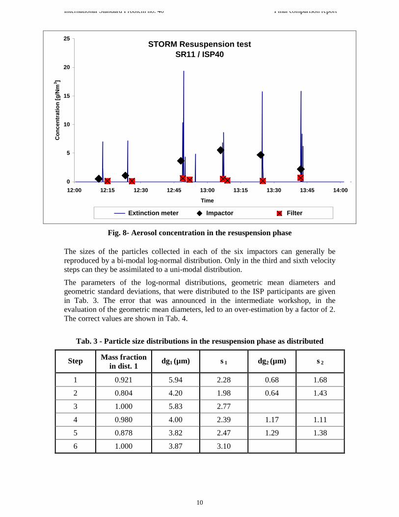
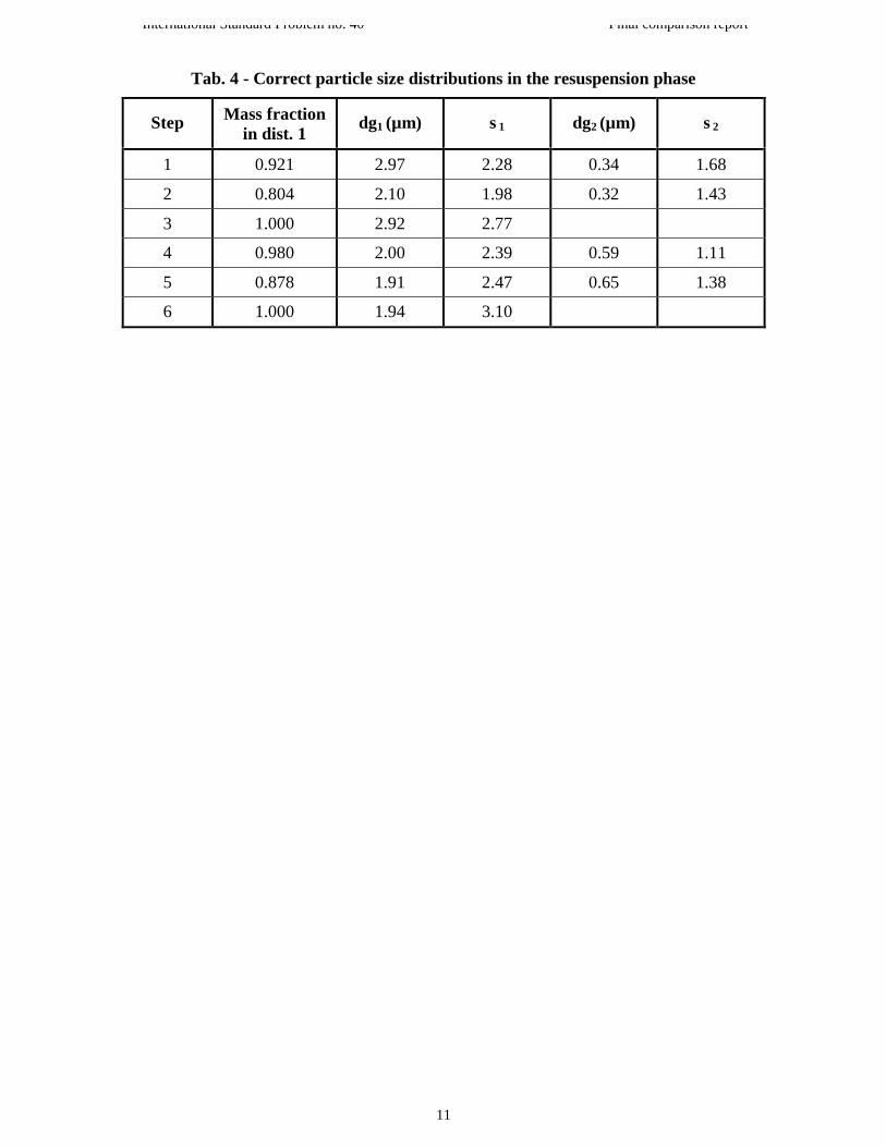

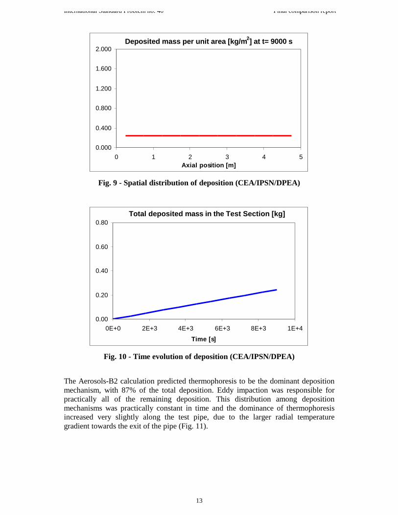


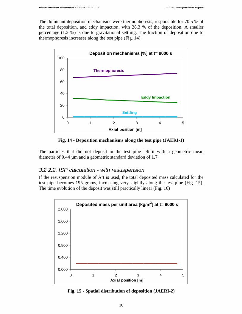


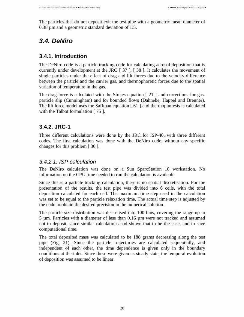
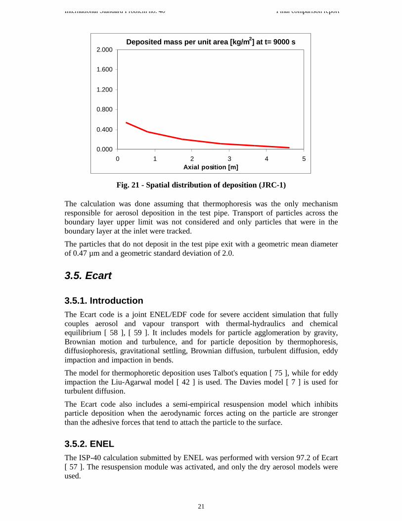


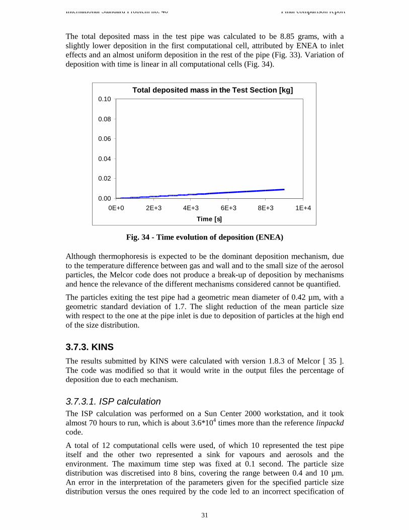
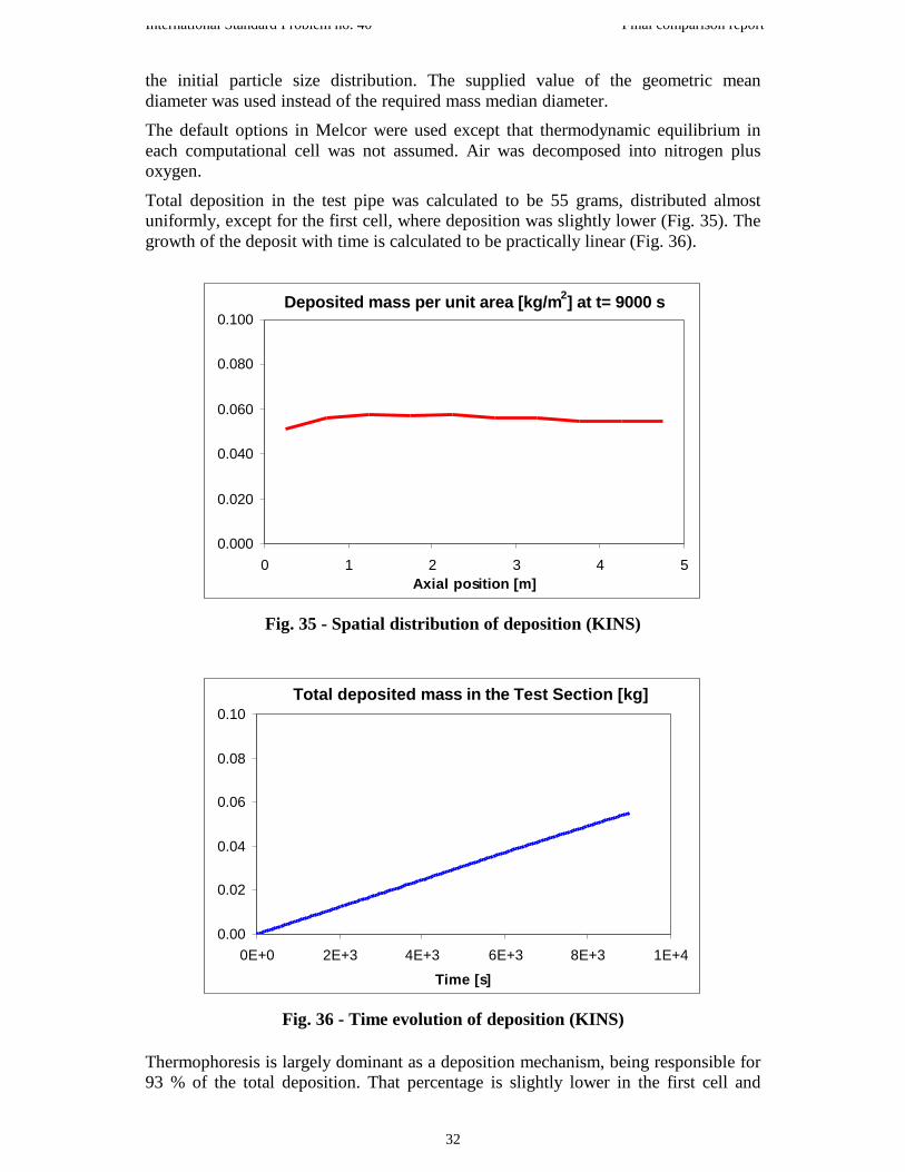


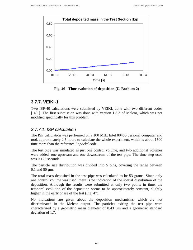


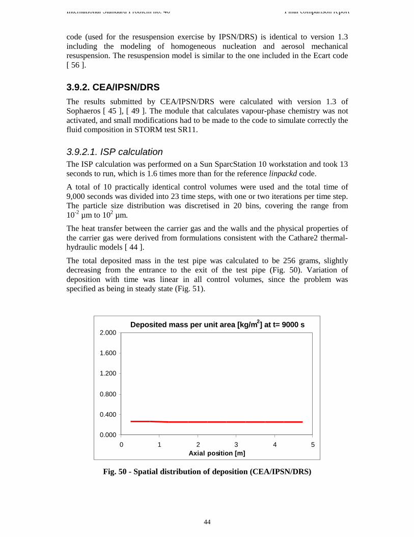


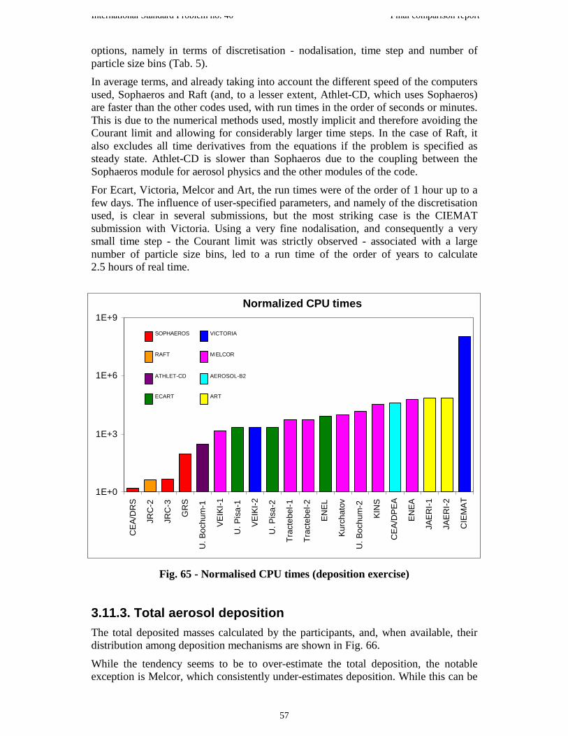


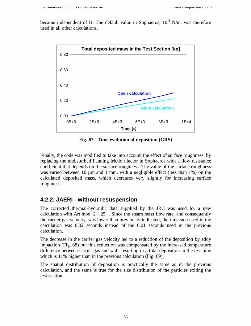

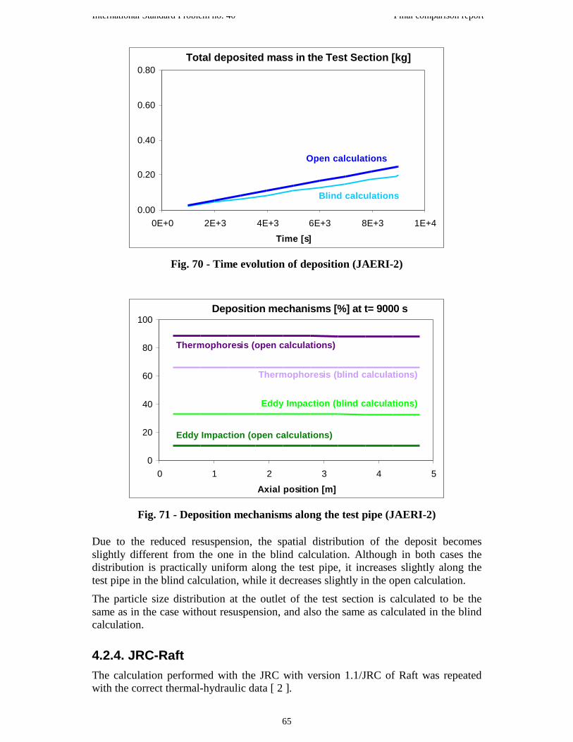


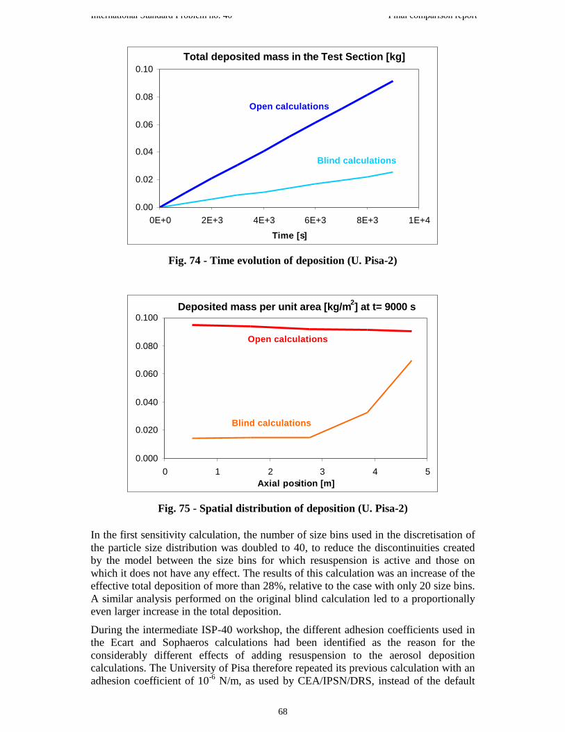


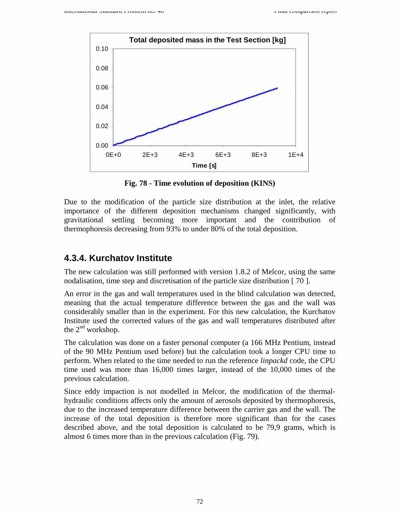


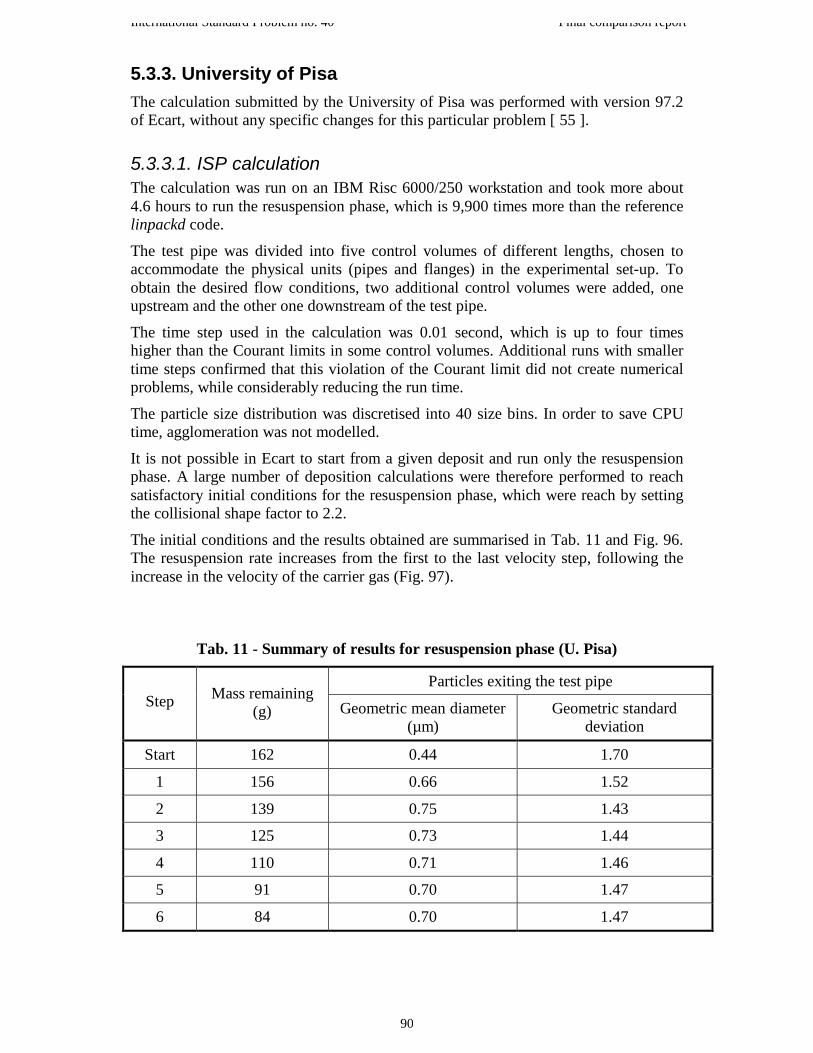


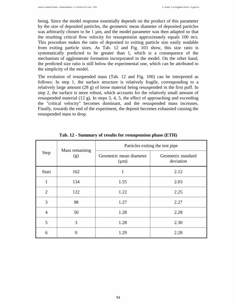


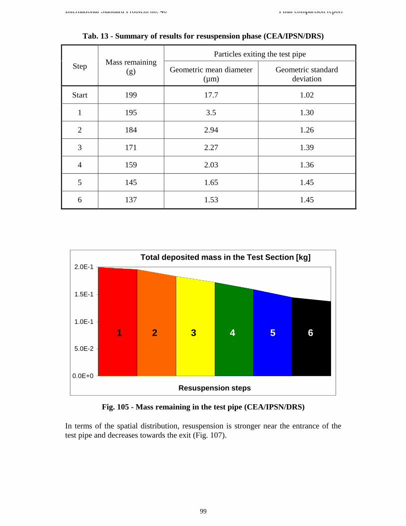


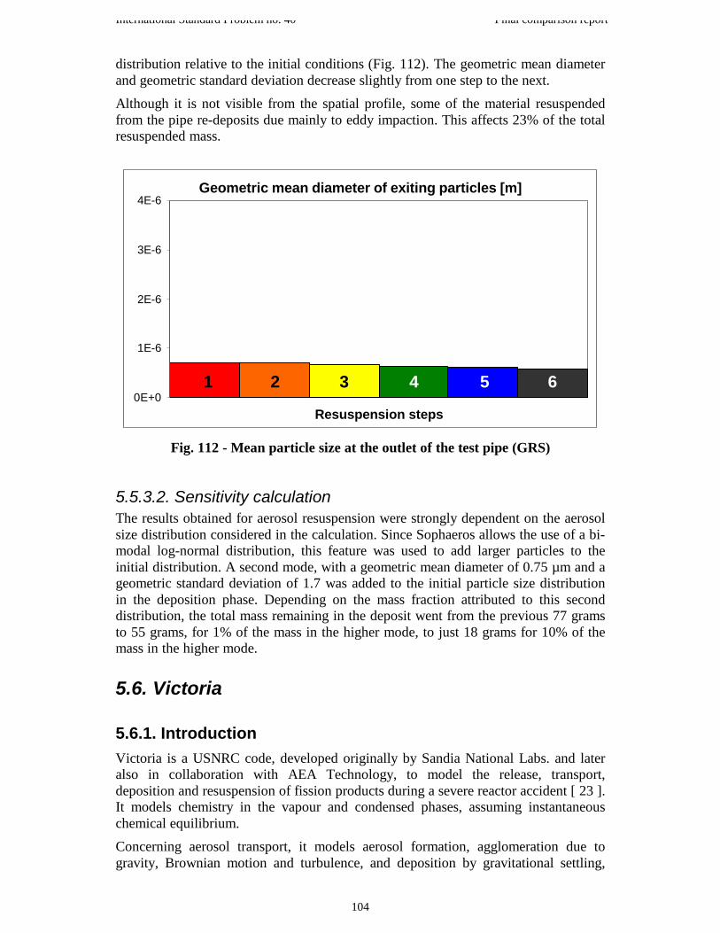


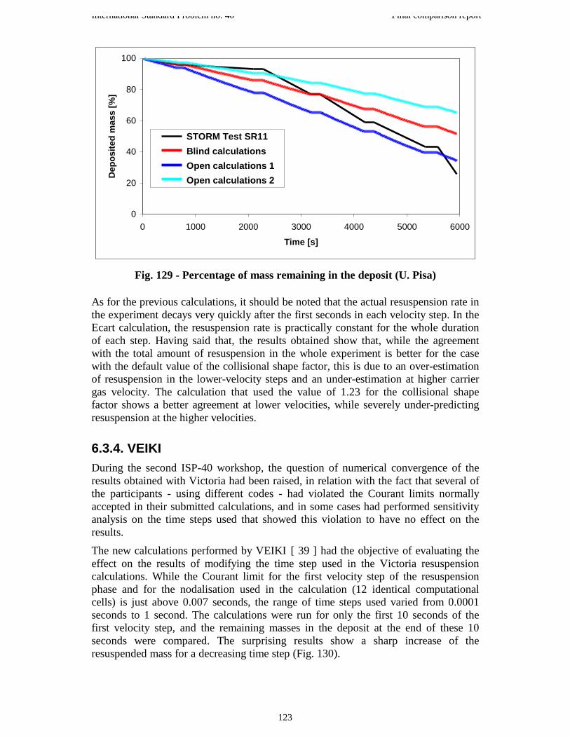


![Aerosol Transport and Conclusions · Aerosol Transport and Deposition ... Microsoft PowerPoint - Particle Transport__Ahmadi_NETL.ppt [Compatibility Mode] Author: gahmadi Created Date:](https://static.documents.pub/doc/80x56/5adef1cb7f8b9a1c248b6b05/aerosol-transport-and-conclusions-transport-and-deposition-microsoft-powerpoint.jpg)


