Introduction - inmabb.criba.edu.arinmabb.criba.edu.ar/revuma/pdf/v55n2/v55n2a02.pdf · algebras H...

REVISTA DE LAUNION MATEMATICA ARGENTINAVol. 55, No. 2, 2014, Pages 11–69Published online: October 13, 2014

HOPF-GALOIS OBJECTS AND COGROUPOIDS

JULIEN BICHON

Abstract. We survey some aspects of the theory of Hopf-Galois objects that

may be studied advantageously by using the language of cogroupoids. These

are the notes for a series of lectures given at Universidad Nacional de Cordoba,May 2010. The lectures are part of the course “Hopf-Galois theory” by Sonia

Natale.

Introduction

These are the notes for a series of lectures given at Universidad Nacional deCordoba, May 2010. The lectures are part of the course “Hopf-Galois theory”by Sonia Natale. We assume therefore some knowledge on Hopf-Galois theory,although some basic facts will be recalled for other readers.

We shall focus on the following two concrete problems. Let H be a Hopf algebra(over a fixed base field k).

(1) Given an H-comodule algebra A that we suspect to be an H-Galois object,how can we prove “nicely” that A is an H-Galois object?

(2) How to classify the H-Galois objects?

Of course these two questions are strongly linked to each other. The answers(or tentative answers) we propose rely on Ulbrich’s [63] equivalence of categoriesbetween the categories of H-Galois objects and fibre functors over the category ofH-comodules.

To answer the first question, we propose here to use the language of cogroupoids.This forces us to introduce more notations and concepts, so what we have to dofirst is to explain our motivation. Recall that an H-Galois object is an H-comodulealgebra for which a certain “canonical” linear map is bijective. The definition isclear and concise, so why should we need to make it more complicated? Of coursethe basic answer, which probably provides enough motivation, is that we want to beable to check that the canonical map is indeed bijective. Another more conceptualmotivation comes with the following parallel situation: given a monoid G, then G

2010 Mathematics Subject Classification. 16W30.The visit at Universidad Nacional de Cordoba was supported by the program Premer-Prefalc

and Conicet (PIP CONICET 112-200801-00566t).

11

12 JULIEN BICHON

is a group if and only if the following “canonical map”

G×G −→ G×G(x, y) 7−→ (xy, y)

is bijective. Of course this gives a short definition of groups that does not use theaxioms of inverses, but for many obvious reasons we prefer to use the (slightly moreinvolved) axioms of inverses. This is exactly the same philosophy that leads to theuse of cogroupoids in Hopf-Galois theory: we will have (much) more axioms but onthe other hand they should be more natural and easier to deal with. We presentvarious examples of cogroupoids (Section 3). We hope that they will convincethe reader that it is not more difficult (and in some sense easier) to work withcogroupoids rather than with Galois objects.

One of the main motivations for studying Hopf-(bi)Galois objects is an importantresult by Schauenburg [53] stating that the comodule categories over two Hopfalgebras H and L are monoidally equivalent if and only if there exists an H-L-bi-Galois object. The knowledge of the full cogroupoid structure (rather than“only” the bi-Galois object) might be useful to exactly determine the image ofan object by the monoidal equivalence. It is also the aim of the notes to presentseveral applications of this: construction of new explicit resolutions from old onesin homological algebra, invariant theory, monoidal equivalences between categoriesof Yetter-Drinfeld modules with applications to bialgebra cohomology and Brauergroups. The use of the cogroupoid structure is probably not necessary everywhere,but we believe that it can help!

The second question that we are concerned with is the classification problem ofthe Hopf-Galois objects of a given Hopf algebra. Once again this is motivated bymonoidal categories of comodules and Ulbrich’s theorem [63] already mentioned.We shall see that in fact Ulbrich’s theorem is, in some situations, a very convenienttool to classify Hopf-Galois objects.

These notes are organized as follows. In Section 1 we recall some basic definitionsand some important results on Hopf-Galois objects. In most cases we do not giveproofs but at some occasions we give parts of the proofs, when these are useful forthe rest of the paper. In Section 2 we introduce cogroupoids and prove some basicresults. We show that a connected cogroupoid induces a bi-Galois object and hencea monoidal equivalence between the comodule categories over two Hopf algebras.Conversely it is shown that any Hopf-Galois object and any monoidal equivalencebetween comodule categories always arises from a connected cogroupoid. We alsoshow that a connected cogroupoid gives rise to a weak Hopf algebra. In Section 3we present various examples of cogroupoids. In Section 4 we use the fibre functormethod (and the constructions of Section 3) to classify the Galois objects over theHopf algebras of bilinear forms and the universal cosovereign Hopf algebras. Sec-tion 5 is devoted to applications of Hopf-Galois objects and monoidal equivalencesto comodule algebras: we describe a model comodule algebra for the Hopf algebraof a bilinear form and we show how to use Hopf-Galois objects to get new resultsfrom old ones in invariant theory. In Section 6 we show how monoidal equivalences

Rev. Un. Mat. Argentina, Vol. 55, No. 2 (2014)

HOPF-GALOIS OBJECTS AND COGROUPOIDS 13

between comodule categories extend to categories of Yetter-Drinfeld modules andwe give an application to Brauer groups of Hopf algebras. Section 7 is devoted toapplications in homological algebra: we show that the Hochshild (co)homology of aHopf-Galois object is determined by the Hochshild (co)homology of the correspond-ing Hopf algebras, we show how to transport equivariant resolutions, and we givean application of the result on Yetter-Drindeld modules to bialgebra cohomology.

These notes are mostly a compilation or reformulation of well-known results.One of the only new results is the construction (Proposition 2.26) of a weak Hopfalgebra from a cogroupoid (hence from a Hopf-Galois object). This (unpublished)result was obtained in collaboration with Grunspan in 2003-2004. A similar resulthas been obtained independently by De Commer [20, 21]. The notions of cocategoryand cogroupoid were presented by the author in several talks between 2004 and2008 (together with the result with Grunspan). It seems to be their first formalappearance in printed form, but of course these notions are so natural that theymight have been defined by any mathematician who would have needed them!

There are many aspects of Hopf-Galois theory (in particular Galois correspon-dences and Hopf-Galois extensions with non-trivial coinvariants) that are ignoredin these notes. The reader might consult the excellent survey papers [47, 54] forthese topics.

Notations and conventions. Throughout these notes we work over a fixed basefield denoted k. We assume that the reader has some knowledge of Hopf algebratheory and Hopf-Galois theory (as in [46], for Hopf-Galois theory we recall all thenecessary definitions) and on monoidal category theory [36]. We use the standardnotations, and in particular Sweedler’s notation ∆(x) = x(1) ⊗ x(2). The categoryof k-vector spaces (resp. finite dimensional k-vector spaces) is denoted Vect(k)(resp. Vectf (k)). The k-linear monoidal category of right H-comodules (resp. finite-dimensional rightH-comodules) over a Hopf algebraH is denoted Comod(H) (resp.Comodf (H)), and the set of H-comodule morphisms (H-colinear maps) betweenH-comodules V , W is denoted HomH(V,W ).

Acknowledgements. It is a pleasure to thank Sonia Natale for the invitation togive these lectures and for her kind hospitality at Cordoba.

1. Background on Hopf-Galois objects

In this section we collect the definitions, constructions and results needed in thepaper.

1.1. Hopf-Galois objects.

Definition 1.1. Let H be a Hopf algebra. A left H-Galois object is a left H-comodule algebra A 6= (0) such that if α : A −→ H ⊗ A denotes the coaction of Hon A, the linear map

κl : A⊗A α⊗1A−−−−→ H ⊗A⊗A 1H⊗m−−−−→ H ⊗A


14 JULIEN BICHON

is an isomorphism. A right H-Galois object is a right H-comodule algebraA 6= (0) such that if β : A −→ A ⊗H denotes the coaction of H on A, the linearmap κr defined by the composition

κr : A⊗A 1A⊗β−−−−→ A⊗A⊗H m⊗1H−−−−→ A⊗His an isomorphism.

If L is another Hopf algebra, an H-L-bi-Galois object is an H-L-bicomodulealgebra which is both a left H-Galois object and a right L-Galois object.

The maps κl and κr are often called the canonical maps.

Example 1.2. The Hopf algebra H, endowed with its comultiplication ∆, is itselfan H-H-bi-Galois object.

Note that if H is a bialgebra, the maps κl and κl are well defined and H is aHopf algebra if and only if κl is bijective if and only if κr is bijective. This givesa definition of Hopf algebras without using the antipode axioms. However, thedefinition with the antipode is much more preferable.

Example 1.3. Let H be a Hopf algebra. Recall (see e.g. [18]) that a 2-cocycleon H is a convolution invertible linear map σ : H ⊗H −→ k satisfying

σ(x(1), y(1))σ(x(2)y(2), z) = σ(y(1), z(1))σ(x, y(2)z(2))

and σ(x, 1) = σ(1, x) = ε(x), for all x, y, z ∈ H. The set of 2-cocycles on H isdenoted Z2(H). When H = k[G] is a group algebra, it is easy to check that wehave an identification Z2(k[G]) ' Z2(G, k∗). Note however that in general there isno natural group structure on Z2(H).

The convolution inverse of σ, denoted σ−1, satisfies

σ−1(x(1)y(1), z)σ−1(x(2), y(2)) = σ−1(x, y(1)z(1))σ

−1(y(2), z(2))

and σ−1(x, 1) = σ−1(1, x) = ε(x), for all x, y, z ∈ H.The algebra σH is defined as follows. As a vector space σH = H and the product

of σH is defined to be

x · y = σ(x(1), y(1))x(2)y(2), x, y ∈ H.That σH is an associative algebra with 1 as unit follows from the 2-cocycle condi-tion. Moreover σH is a right H-comodule algebra with ∆ : σH −→ σH ⊗ H as acoaction, and is a right H-Galois object.

Similarly we have the algebra Hσ−1 . As a vector space Hσ−1 = H and theproduct of Hσ−1 is defined to be

x · y = σ−1(x(2), y(2))x(1)y(1), x, y ∈ H.Then Hσ−1 is a left H-comodule algebra with coaction ∆ : Hσ−1 −→ H ⊗ Hσ−1

and Hσ−1 is a left H-Galois object. We will (re)prove these facts in Subsection 3.3.

Example 1.4. Let H be a Hopf algebra and let A be a left H-Galois object withcoaction α : A −→ H ⊗ A, α(a) = a(−1) ⊗ a(0). Then the linear map β : Aop −→Aop ⊗ H, β(a) = a(0) ⊗ S(a(−1)) endows Aop with a right H-comodule algebrastructure, and Aop is right H-Galois if the antipode S is bijective (exercise).



Hence if the antipode of H is bijective, there is no essential difference betweenleft anf right H-Galois objects.

Definition 1.5. Let H be a Hopf algebra. The category of left H-Galois ob-jects (resp. right H-Galois objects), denoted Gall(H) (resp. Galr(H)), is thecategory whose objects are left H-Galois objects (resp. right H-Galois objects) andwhose morphisms are H-colinear algebra maps (i.e. H-comodule algebra maps).

The set of isomorphism classes of left H-Galois objects (resp. right H-Galois

objects) is denoted Gall(H) (resp. Galr(H)).

It follows from Example 1.4 that if H has bijective antipode, the categoriesGall(H) and Galr(H) are isomorphic, and in this case we simply put Gal(H) =

Gall(H) = Galr(H).

The following result (Remark 3.11 in [55]), means that the categories Gall(H)and Galr(H) are groupoids (i.e. every morphism is an isomorphism). It is veryuseful for classification results.

Proposition 1.6. Let H be a Hopf algebra and let A, B some (left or right)H-Galois objects. Any H-colinear algebra map f : A −→ B is an isomorphism.

Proof. Assume for example that A and B are left H-Galois and denote by κAl andκBl the respective canonical maps. Endow B with the left A-module structureinduced by f . The diagram

A⊗B κBl (f⊗1B)−−−−−−−→ H ⊗B

'y '

y(A⊗A)⊗A B

κAl ⊗A1B−−−−−−→ (H ⊗A)⊗A Bcommutes and hence f ⊗ 1B is an isomorphism, and so is f .

We get a simple criterion to test if a Galois object is trivial.

Proposition 1.7. Let H be a Hopf algebra and let A be a left or right H-Galoisobject. Then A ∼= H as H-comodule algebras if and only if there exists an algebramap φ : A −→ k.

Proof. It is clear, using the counit, that if A ∼= H as comodule algebras, then thereexists an algebra map A −→ k. Conversely, assume for example that A is left H-galois and that there exists an algebra map φ : A −→ k. Then the map A −→ H,a 7−→ φ(a(0))a(−1) is a left H-colinear algebra map, and is an isomorphism by theprevious proposition.

1.2. Cleft Hopf-Galois objects. In this subsection we briefly focus on an im-portant class of Hopf-Galois objects, called cleft.

We have already seen (Example 1.3) how to associate a Galois object to a 2-cocyle. This construction is axiomatized by the following result, which summarizeswork of Doi-Takeuchi [19] and Blattner-Montgomery [14]. The proof can be foundin [46] or [54].


16 JULIEN BICHON

Theorem 1.8. Let H be a Hopf algebra and let A be a left H-Galois object. Thefollowing assertions are equivalent:

(1) There exists σ ∈ Z2(H) such that A ∼= Hσ−1 as left comodule algebras.(2) A ∼= H as left H-comodules.(3) There exists a convolution invertible H-colinear map φ : H −→ A

A left H-Galois object is said to be cleft if it satisfies the above equivalent condi-tions.

Of course there is a similar result for right H-Galois objects.There are nice classes of Hopf algebras for which cleftness is automatic. Re-

call that a Hopf algebra is said to be pointed if all its simple comodules are 1-dimensional.

Theorem 1.9. Let H be a finite-dimensional or pointed Hopf algebra. Then anyH-Galois object is cleft.

For the pointed case we refer the reader to Remark 10 in [31] and for the finite-dimensional case we refer the reader to [40]. See however the last remark in thenext subsection, where we give a proof by using fibre functors.

1.3. Monoidal equivalences and Schauenburg’s theorem. The following re-sult from [53] is one of the main motivations for the study of (bi-)Galois objects.

Theorem 1.10 (Schauenburg). Let H and L be some Hopf algebras. The followingassertions are equivalent.

(1) There exists a k-linear equivalence of monoidal categories

Comod(H) ∼=⊗ Comod(L).

(2) There exists an H-L-bi-Galois object.

So we have a very powerful tool to construct monoidal equivalences betweencategories of comodules over Hopf algebras! In the next subsection we presentvarious very important constructions related to Schauenburg’s theorem.

1.4. Cotensor product and various constructions of functors. In this sub-section we recall several important constructions of functors associated with Hopf-Galois objects. The basic construction is the cotensor product.

Definition 1.11. Let C be a coalgebra, let V be a right C-comodule and let Wbe a left C-comodule. The cotensor product of V and W , denoted VCW , isdefined to be the equalizer

0 −→ VCW −→ V ⊗W ⇒ V ⊗ C ⊗W,

i.e. the kernel of the map αV ⊗1W −1V ⊗αW , where αV and αW are the respectivecoactions on V and W .

The first thing that the cotensor product allows us to do is to construct functorson comodule categories, as follows.



Proposition 1.12. Let C be a coalgebra. Any left C-comodule W defines a k-linearfunctor

ΩW : Comod(C) −→ Vect(k)

V 7−→ VCW.

Proof. If f : V −→ V ′ is C-colinear map, then it is easy to check that f ⊗1(VCW ) ⊂ V ′CW and hence we get the announced functor.

Remark 1.13. If W ∼= C as left C-comodules, then ΩW is isomorphic to theforgetful functor.

Proof. Let f : C −→W be a C-colinear isomorphism. If V is a right C-comodule,we have a vector space isomorphism

V −→ VCW = ΩW (V )

v 7−→ v(0) ⊗ f(v(1))

(the inverse is given by v⊗a 7→ ε(f−1(a))v). The isomorphism is clearly functorialand we have the result.

The monoidal analogue of Proposition 1.12 is Ulbrich’s theorem [63]:

Theorem 1.14 (Ulbrich). Let H be a Hopf algebra and let A be a left H-Galoisobject. The functor

ΩA : Comodf (H) −→ Vectf (k)

V 7−→ VHA

is a fibre functor: it is k-linear, exact, faithful and monoidal. Conversely, any fibrefunctor arises in this way from a unique (up to isomorphism) left H-Galois object.

Partial proof. Consider the previous functor ΩA : Comod(H) −→ Vect(k). Weendow ΩA with a monoidal structure as follows (the construction is from [62]).

First define ΩA0 : k −→ ΩA(k) = kHA = AcoH , 1 7−→ 1. This is an isomorphismsince for a ∈ AcoH , we have κl(a⊗1) = 1⊗a = κl(1⊗a), hence we have a⊗1 = 1⊗aby the injectivity of κl and a ∈ k1.

Now let V,W ∈ Comod(H). It is straightforward to check that if∑i vi ⊗ ai ∈

VHA and∑j wj ⊗ bj ∈WHA, then∑

i,j

vi ⊗ wj ⊗ aibj ∈ (V ⊗W )HA.

Thus we have a map

(VHA)⊗ (WHA) −→ (V ⊗W )HA

(∑i

vi ⊗ ai)⊗ (∑j

wj ⊗ bj) 7−→∑i,j

vi ⊗ wj ⊗ aibj

that we denote

ΩAV,W : ΩA(V )⊗ ΩA(W ) −→ ΩA(V ⊗W )


18 JULIEN BICHON

It is clear that this map is functorial, and we have to check that ΩA = (ΩA, ΩA•,•, ΩA0 )

is a monoidal functor. It is easy to seen that the associativity (coherence) con-straints of a monoidal functor are satisfied, and what is really non trivial is to

check that ΩAV,W is an isomorphism for any V,W ∈ Comod(H). We use the follow-ing Lemma.

Lemma 1.15.

(1) For any V ∈ Comod(H), the linear map 1⊗ε⊗1 : (V ⊗H)HA −→ V ⊗Ais an isomorphism.

(2) For any V ∈ Comod(H), the linear map mV := 1⊗m : (VHA)⊗A −→V ⊗A is an isomorphism.

Proof of the Lemma. (1) The reader will easily check that the inverse V ⊗ A −→(V ⊗H)HA is given by v ⊗ a 7−→ v(0) ⊗ S(v(1))a(−1) ⊗ a(0).

(2) It is not difficult to check that 1 ⊗ κl : V ⊗ A ⊗ A −→ V ⊗H ⊗ A inducesa map 1 ⊗ κl : (VHA) ⊗ A −→ (VHH) ⊗ A and that the following diagramcommutes

(VHA)⊗A

mV''NNNNNNNNNNN1⊗κl // (VHH)⊗A

1⊗ε⊗1

wwppppppppppp

V ⊗Awith the vertical arrow on the right bijective by (1), so mV is an isomorphism.

We are now ready to prove that ΩAV,W is an isomorphism. The following diagramcommutes

(VHA)⊗ (WHA)⊗A

1⊗mW

ΩAV,W⊗1// ((V ⊗W )HA)⊗A

mV⊗W

(VHA)⊗W ⊗A 1⊗τ // (VHA)⊗A⊗W mV ⊗1 // V ⊗A⊗W

1⊗τ // V ⊗W ⊗A

where the τ ’s denote the canonical flips x ⊗ y 7→ y ⊗ x. Since by the Lemmaall the vertical and horizontal down morphisms are isomorphisms we conclude

that ΩAV,W ⊗ 1 is an isomorphism, and so is ΩAV,W : we have our monoidal functor

ΩA = (ΩA, ΩA•,•, ΩA0 ) : Comod(H) −→ Vect(k). That ΩA : Comod(H) −→ Vect(k)

restricts to a monoidal functor ΩA : Comodf (H) −→ Vectf (k) is a consequence ofthe forthcoming Proposition 1.16.

Faithfulness of ΩA is obvious while exactness is easy using (2) in the Lemma (see[62]), hence ΩA is a fibre functor. We do not prove the converse (see [62, 63]).

The following result has been used in the partial proof of Ulbrich’s theorem andwill also be useful elsewhere.

Proposition 1.16. Let H be a Hopf algebra and let F : Comod(H) −→ Vect(k)be a monoidal functor. If V is a finite-dimensional H-comodule, then F (V ) is afinite-dimensional vector space. Moreover we have dim(V ) = 1⇒ dim(F (V )) = 1,and if F is a fibre functor then dim(F (V )) = 1⇒ dim(V ) = 1.



Proof. The key point is that a vector space V is finite-dimensional if and only ifthere exists a vector space W and linear maps e : W ⊗ V → k and d : k → V ⊗Wsuch that

1V = (1V ⊗ e) (d⊗ 1V ), 1W = (e⊗ 1W ) (1W ⊗ d).

If V ∈ Comodf (H), the dual comodule V ∗ satisfies to the above requirement withe and d H-colinear, where e is the evaluation map: in other words V has a left dualin Comod(H), see [34] or [36]. Applying the monoidal functor F , we easily see thatF (V ) satisfies to the above condition and hence that F (V ) is finite-dimensional.If dim(V ) = 1, then e : V ∗ ⊗ V −→ k is an isomorphism and so is the inducedcomposition F (V ∗) ⊗ F (V ) ∼= F (V ∗ ⊗ V ) ∼= F (k) ∼= k, hence dim(F (V )) = 1.If dim(F (V )) = 1, then the previous composition is an isomorphism (becausethe monoidal functor transforms left duals into left duals), and hence F (e) is anisomorphism. If F is a fibre functor then it is exact faithful so e is an isomorphism,which shows that dim(V ) = 1.

Of course there is a left-right version of Ulbrich’s theorem. Note that Ulbrich’stheorem in [63] is a stronger statement: it states an equivalence of categories be-tween left H-Galois objects and fibre functors on Comodf (H).

In the setting of fibre functors there is a nice characterization of cleftness interms of fibre functors, essentially due to Etingof-Gelaki [24].

Theorem 1.17. Let H be a Hopf algebra and let A be a left H-Galois object. Thefollowing assertions are equivalent.

(1) A is a cleft H-Galois object.(2) The fibre functor ΩA : Comodf (H) −→ Vectf (k) preserves the dimensions

of the underlying vector spaces.

Partial proof. We give the proof of (1)⇒ (2) (the easy part) and we refer to [24] forthe proof of (2)⇒ (1). If A is cleft there exists an H-colinear isomorphism H ∼= Aand by Remark 1.13 ΩA is isomorphic to the forgetful functor, which proves theresult.

Remark 1.18. We can use the fibre functor interpretation to give a proof ofTheorem 1.9. Let A be a left H-Galois object.

Assume first that H is pointed. Any simple H-comodule is one dimensional, soΩA preserves the dimension of any simple H-comodule by Proposition 1.16. Aninduction now shows that ΩA preserves the dimension of any finite-dimensionalH-comodule, and hence A is cleft by Theorem 1.17.

Assume now that H is finite-dimensional. We have a linear isomorphism A ∼=HHA = ΩA(H), a 7→ a(−1) ⊗ a(0), so A is finite-dimensional since ΩA has itsvalues in Vectf (k). Denote by A0 the trivial H-comodule whose underlying vectorspace is A. The canonical map κl : A ⊗ A0 −→ H ⊗ A0 is a left H-comoduleisomorphism. Hence we have a left H-comodule isomorphism Adim(A) ∼= Hdim(A)

and so the Krull-Schmidt theorem shows that A ∼= H as left H-comodules.

We now come to the construction of functors between categories of comodules.The basic result is the following one.


20 JULIEN BICHON

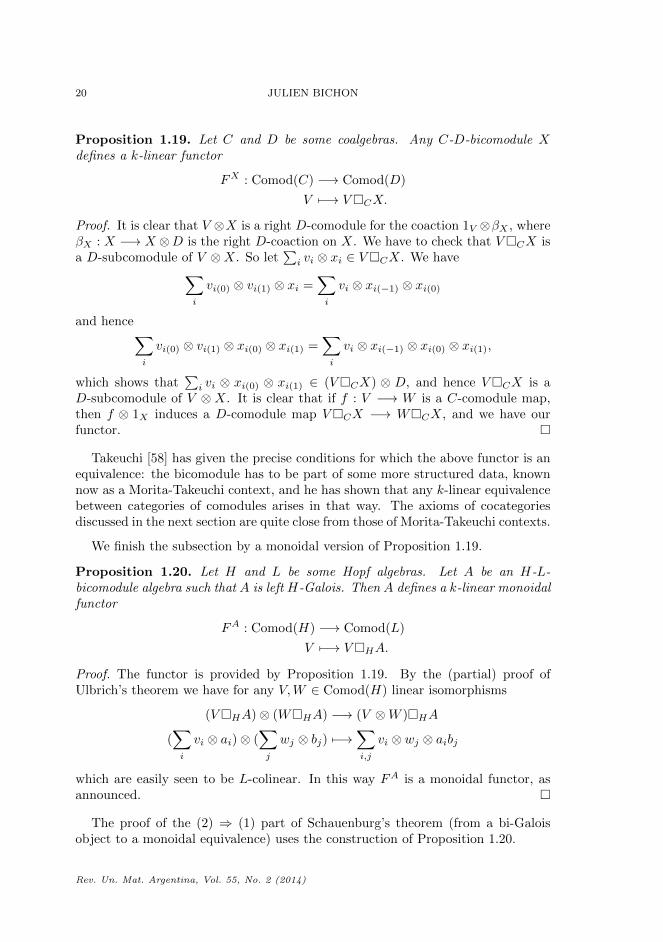
Proposition 1.19. Let C and D be some coalgebras. Any C-D-bicomodule Xdefines a k-linear functor

FX : Comod(C) −→ Comod(D)

V 7−→ VCX.

Proof. It is clear that V ⊗X is a right D-comodule for the coaction 1V ⊗βX , whereβX : X −→ X ⊗D is the right D-coaction on X. We have to check that VCX isa D-subcomodule of V ⊗X. So let

∑i vi ⊗ xi ∈ VCX. We have∑

i

vi(0) ⊗ vi(1) ⊗ xi =∑i

vi ⊗ xi(−1) ⊗ xi(0)

and hence∑i

vi(0) ⊗ vi(1) ⊗ xi(0) ⊗ xi(1) =∑i

vi ⊗ xi(−1) ⊗ xi(0) ⊗ xi(1),

which shows that∑i vi ⊗ xi(0) ⊗ xi(1) ∈ (VCX) ⊗ D, and hence VCX is a

D-subcomodule of V ⊗ X. It is clear that if f : V −→ W is a C-comodule map,then f ⊗ 1X induces a D-comodule map VCX −→ WCX, and we have ourfunctor.

Takeuchi [58] has given the precise conditions for which the above functor is anequivalence: the bicomodule has to be part of some more structured data, knownnow as a Morita-Takeuchi context, and he has shown that any k-linear equivalencebetween categories of comodules arises in that way. The axioms of cocategoriesdiscussed in the next section are quite close from those of Morita-Takeuchi contexts.

We finish the subsection by a monoidal version of Proposition 1.19.

Proposition 1.20. Let H and L be some Hopf algebras. Let A be an H-L-bicomodule algebra such that A is left H-Galois. Then A defines a k-linear monoidalfunctor

FA : Comod(H) −→ Comod(L)

V 7−→ VHA.

Proof. The functor is provided by Proposition 1.19. By the (partial) proof ofUlbrich’s theorem we have for any V,W ∈ Comod(H) linear isomorphisms

(VHA)⊗ (WHA) −→ (V ⊗W )HA

(∑i

vi ⊗ ai)⊗ (∑j

wj ⊗ bj) 7−→∑i,j

vi ⊗ wj ⊗ aibj

which are easily seen to be L-colinear. In this way FA is a monoidal functor, asannounced.

The proof of the (2) ⇒ (1) part of Schauenburg’s theorem (from a bi-Galoisobject to a monoidal equivalence) uses the construction of Proposition 1.20.



2. Cocategories and cogroupoids

In this section we put Hopf bi-Galois objects into a more structured framework.The idea is that although the axiomatic becomes more complicated at first sight,it should be more natural and easier to deal with.

2.1. Basic definitions. The first step is to propose a notion that is dual to theone of category, as follows.

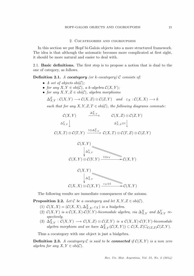
Definition 2.1. A cocategory (or k-cocategory) C consists of:

• A set of objects ob(C);• for any X,Y ∈ ob(C), a k-algebra C(X,Y );• for any X,Y, Z ∈ ob(C), algebra morphisms

∆ZX,Y : C(X,Y ) −→ C(X,Z)⊗ C(Z, Y ) and εX : C(X,X) −→ k

such that for any X,Y, Z, T ∈ ob(C), the following diagrams commute:

C(X,Y )∆ZX,Y−−−−→ C(X,Z)⊗ C(Z, Y )

∆TX,Y

y ∆TX,Z⊗1

yC(X,T )⊗ C(T, Y )

1⊗∆ZT,Y−−−−−→ C(X,T )⊗ C(T,Z)⊗ C(Z, Y )

C(X,Y )

∆YX,Y

TTTTTTTTTTTTTTTTT

TTTTTTTTTTTTTTTTT

C(X,Y )⊗ C(Y, Y )1⊗εY // C(X,Y )

C(X,Y )

∆XX,Y

TTTTTTTTTTTTTTTTT

TTTTTTTTTTTTTTTTT

C(X,X)⊗ C(X,Y )εX⊗1 // C(X,Y )

The following results are immediate consequences of the axioms.

Proposition 2.2. Let C be a cocategory and let X,Y, Z ∈ ob(C).(1) C(X,X) = (C(X,X),∆X

X,X , εX) is a bialgebra.

(2) C(X,Y ) is a C(X,X)-C(Y, Y )-bicomodule algebra, via ∆XX,Y and ∆Y

X,Y re-spectively.

(3) ∆ZX,Y : C(X,Y ) −→ C(X,Z) ⊗ C(Z, Y ) is a C(X,X)-C(Y, Y )-bicomodule

algebra morphism and we have ∆ZX,Y (C(X,Y )) ⊂ C(X,Z)C(Z,Z)C(Z, Y ).

Thus a cocategory with one object is just a bialgebra.

Definition 2.3. A cocategory C is said to be connected if C(X,Y ) is a non zeroalgebra for any X,Y ∈ ob(C).


22 JULIEN BICHON

A groupoid is a category whose morphisms all are isomorphisms. A dual notionis the following one.

Definition 2.4. A cogroupoid (or a k-cogroupoid) C consists of a cocategory Ctogether with, for any X,Y ∈ ob(C), linear maps

SX,Y : C(X,Y ) −→ C(Y,X)

such that for any X,Y ∈ ob(C), the following diagrams commute:

C(X,X)εX //

∆YX,X

ku // C(X,Y )

C(X,Y )⊗ C(Y,X)1⊗SY,X // C(X,Y )⊗ C(X,Y )

m

OO

C(X,X)εX //

∆YX,X

ku // C(Y,X)

C(X,Y )⊗ C(Y,X)SX,Y ⊗1 // C(Y,X)⊗ C(Y,X)

m

OO

where m denotes the multiplication of C(X,Y ) and u is the unit map.

It follows immediately that if C is a cogroupoid and X ∈ ob(C), then C(X,X) isa Hopf algebra.

Remark 2.5 (on terminology). A connected cogroupoid with two objects is ex-actly what Grunspan called a total Hopf-Galois system in [29] (some axioms areredundant in [29]), which was a symmetrisation of the notion of Hopf-Galois sys-tem from [11]. It seems that the more compact present formulation is much moreconvenient and pleasant to deal with.

Definition 2.6. A full subcocategory (resp. full subcogroupoid) of a cocate-gory (resp. cogroupoid) C is a cocategory (resp. cogroupoid) D with ob(D) ⊂ ob(C),with D(X,Y ) = C(X,Y ), ∀X,Y ∈ ob(D), and whose structural morphisms arethose induced by the ones of C.

Notation 2.7. We now introduce Sweedler’s notation for cocategories and cogroup-oids. Let C be a cocategory. For aX,Y ∈ C(X,Y ), we write

∆ZX,Y (aX,Y ) = aX,Z(1) ⊗ a

Z,Y(2) .

The cocategory axioms now read

(∆TX,Z ⊗ 1) ∆Z

X,Y (aX,Y ) = aX,T(1) ⊗ aT,Z(2) ⊗ a

Z,Y(3) = (1⊗∆Z

T,Y ) ∆TX,Y (aX,Y ),

εX(aX,X(1) )aX,Y(2) = aX,Y = εY (aY,Y(2) )aX,Y(1) ,

and the additional cogroupoid axioms are

SX,Y (aX,Y(1) )aY,X(2) = εX(aX,X)1 = aX,Y(1) SY,X(aY,X(2) ).



2.2. Back to Hopf-Galois objects.

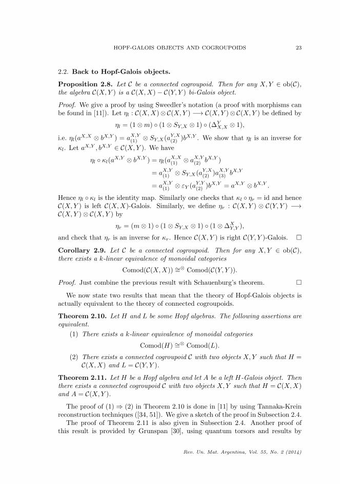
Proposition 2.8. Let C be a connected cogroupoid. Then for any X,Y ∈ ob(C),the algebra C(X,Y ) is a C(X,X)− C(Y, Y ) bi-Galois object.

Proof. We give a proof by using Sweedler’s notation (a proof with morphisms canbe found in [11]). Let ηl : C(X,X)⊗C(X,Y ) −→ C(X,Y )⊗C(X,Y ) be defined by

ηl = (1⊗m) (1⊗ SY,X ⊗ 1) (∆YX,X ⊗ 1),

i.e. ηl(aX,X ⊗ bX,Y ) = aX,Y(1) ⊗ SY,X(aY,X(2) )bX,Y . We show that ηl is an inverse for

κl. Let aX,Y , bX,Y ∈ C(X,Y ). We have

ηl κl(aX,Y ⊗ bX,Y ) = ηl(aX,X(1) ⊗ a

X,Y(2) bX,Y )

= aX,Y(1) ⊗ SY,X(aY,X(2) )aX,Y(3) bX,Y

= aX,Y(1) ⊗ εY (aY,Y(2) )bX,Y = aX,Y ⊗ bX,Y .

Hence ηl κl is the identity map. Similarly one checks that κl ηr = id and henceC(X,Y ) is left C(X,X)-Galois. Similarly, we define ηr : C(X,Y ) ⊗ C(Y, Y ) −→C(X,Y )⊗ C(X,Y ) by

ηr = (m⊗ 1) (1⊗ SY,X ⊗ 1) (1⊗∆XY,Y ),

and check that ηr is an inverse for κr. Hence C(X,Y ) is right C(Y, Y )-Galois.

Corollary 2.9. Let C be a connected cogroupoid. Then for any X,Y ∈ ob(C),there exists a k-linear equivalence of monoidal categories

Comod(C(X,X)) ∼=⊗ Comod(C(Y, Y )).

Proof. Just combine the previous result with Schauenburg’s theorem.

We now state two results that mean that the theory of Hopf-Galois objects isactually equivalent to the theory of connected cogroupoids.

Theorem 2.10. Let H and L be some Hopf algebras. The following assertions areequivalent.

(1) There exists a k-linear equivalence of monoidal categories

Comod(H) ∼=⊗ Comod(L).

(2) There exists a connected cogroupoid C with two objects X,Y such that H =C(X,X) and L = C(Y, Y ).

Theorem 2.11. Let H be a Hopf algebra and let A be a left H-Galois object. Thenthere exists a connected cogroupoid C with two objects X,Y such that H = C(X,X)and A = C(X,Y ).

The proof of (1)⇒ (2) in Theorem 2.10 is done in [11] by using Tannaka-Kreinreconstruction techniques ([34, 51]). We give a sketch of the proof in Subsection 2.4.

The proof of Theorem 2.11 is also given in Subsection 2.4. Another proof ofthis result is provided by Grunspan [30], using quantum torsors and results by


24 JULIEN BICHON

Schauenburg (see [53] and Subsection 2.8 of [54]). This proof has the merit to workfor Hopf algebras over rings (of course with flatness assumptions).

The proofs of these two results in Subsection 2.4 will never be used in the restof the paper, so the reader might skip them first, and get back if he needs to.

The (2) ⇒ (1) part in Theorem 2.10 is the previous corollary. We shall givea proof of it without using Schauenburg’s theorem in the next subsection. Moreprecisely, the explicit form of the monoidal equivalence constructed by startingfrom a connected cogroupoid is as follows. Having this explicit form in hand isuseful in some applications.

Theorem 2.12. Let C be a connected cogroupoid. Then for any X,Y ∈ ob(C) wehave k-linear equivalences of monoidal categories that are inverse of each other

Comod(C(X,X)) ∼=⊗ Comod(C(Y, Y )) Comod(C(Y, Y )) ∼=⊗ Comod(C(X,X))

V 7−→ VC(X,X)C(X,Y ) V 7−→ VC(Y,Y )C(Y,X).

We give a proof in the next subsection.

2.3. Some basic properties of cogroupoids. This section is devoted to statingand proving basic properties of cogroupoids, and to giving a proof of Theorem 2.12.

We begin by examining some properties of the “antipodes”. Part (1) of thefollowing result is proved very indirectly in [11], with a direct proof given in [33].In view of the next Proposition 2.26, these properties also are consequences ofresults on weak Hopf algebras [15].

Proposition 2.13. Let C be a cogroupoid and let X,Y ∈ ob(C).

(1) SY,X : C(Y,X) −→ C(X,Y )op is an algebra morphism.(2) For any Z ∈ ob(C) and aY,X ∈ C(Y,X), we have

∆ZX,Y (SY,X(aY,X)) = SZ,X(aZ,X(2) )⊗ SY,Z(aY,Z(1) ).

Proof. Let aY,X , bY,X ∈ C(Y,X). We have

SY,X(aY,XbY,X) = SY,X(aY,X(1) bY,X(1) )εX(aX,X(2) )εX(bX,X(2) )

= SY,X(aY,X(1) bY,X(1) )aX,Y(2) bX,Y(2) SY,X(bY,X(3) )SY,X(aY,X(3) )

= εY (aY,Y(1) bY,Y(1) )SY,X(bY,X(2) )SY,X(aY,X(2) )

= SY,X(bY,X)SY,X(aY,X),

and this proves (1). We also have

SZ,X(aZ,X(2) )⊗ SY,Z(aY,Z(1) ) = SZ,X(aZ,X(2) εX(aX,X(3) ))⊗ SY,Z(aY,Z(1) )

= SZ,X(aZ,X(2) )⊗ SY,Z(aY,Z(1) ) ·(εX(aX,X(3) )1⊗ 1

)= SZ,X(aZ,X(2) )⊗ SY,Z(aY,Z(1) ) ·

(∆ZX,Y (aX,Y(3) SY,X(aY,X(4) ))

)Rev. Un. Mat. Argentina, Vol. 55, No. 2 (2014)


= SZ,X(aZ,X(2) )⊗ SY,Z(aY,Z(1) ) ·(aX,Z(3) ⊗ a

Z,Y(4)

)·∆Z

X,Y (SY,X(aY,X(5) ))

= εZ(aZ,Z(2) )1⊗ SY,Z(aY,Z(1) )aZ,Y(3) ·∆ZX,Y (SY,X(aY,X(4) ))

= 1⊗ SY,Z(aY,Z(1) )aZ,Y(2) ·∆ZX,Y (SY,X(aY,X(3) ))

= ∆ZX,Y (SY,X(aY,X)),

and this proves (2).

The following result is useful to prove connectedness properties of cogroupoids,and also for the proof of Theorem 2.12.

Lemma 2.14. Let C be a cogroupoid and let X,Y, Z ∈ ob(C). Assume thatC(Z, Y ) 6= (0) or C(X,Z) 6= (0). Then ∆Z

X,Y : C(X,Y ) −→ C(X,Z) ⊗ C(Z, Y )

is split injective, and induces a C(X,X)−C(Y, Y )-bicomodule algebra isomorphism

C(X,Y ) ∼= C(X,Z)C(Z,Z)C(Z, Y ).

Proof. Assume first that C(Z, Y ) 6= (0), and let ψ : C(Z, Y ) −→ k be a linear mapsuch that ψ(1) = 1. Define f : C(X,Z)⊗ C(Z, Y ) −→ C(X,Y ) by

f(aX,Z ⊗ bZ,Y ) = ψ(SY,Z(aY,Z(2) )bZ,Y

)aX,Y(1) .

Then

f ∆ZX,Y (aX,Y ) = f(aX,Z(1) ⊗ a

Z,Y(2) ) = ψ

(SY,Z(aY,Z(2) )aZ,Y(3)

)aX,Y(1)

= εY (aY,Y(2) )aX,Y(1) = aX,Y .

This proves that ∆ZX,Y is split injective. We know from Proposition 2.2 that ∆Z

X,Y

is a C(X,X)-C(Y, Y )-bicomodule algebra morphism and that ∆ZX,Y (C(X,Y )) ⊂

C(X,Z)C(Z,Z)C(Z, Y ). Let∑i aX,Zi ⊗ bZ,Yi ∈ C(X,Z)C(Z,Z)C(Z, Y ). We have

∆ZX,Y f(

∑i

aX,Zi ⊗ bZ,Yi ) = ∆ZX,Y

(∑i

ψ(SY,Z(aY,Zi(2))b

Z,Yi

)aX,Yi(1)

)=∑i

ψ(SY,Z(aY,Zi(3))b

Z,Yi

)aX,Zi(1) ⊗ a

Z,Xi(2)

=∑i

ψ(SY,Z(bY,Zi(2))b

Z,Yi(3)

)aX,Zi ⊗ bZ,Yi(1)

=∑i

εY (bY,Yi(2) )aX,Zi(1) ⊗ bZ,Yi(1) =

∑i

aX,Zi ⊗ bZ,Yi ,

which proves the result. Assume now that C(X,Z) 6= (0), and let φ : C(X,Z) −→ kbe a linear map such that φ(1) = 1. Define g : C(X,Z)⊗ C(Z, Y ) −→ C(X,Y ) by

g(aX,Z ⊗ bZ,Y ) = φ(aX,ZSZ,X(bZ,X(1) )

)bX,Y(2) .


26 JULIEN BICHON

Then

g ∆ZX,Y (aX,Y ) = g(aX,Z(1) ⊗ a

Z,Y(2) ) = φ

(aX,Z(1) SZ,X(aZ,X(2) )

)aX,Y(3)

= εX(aX,X(1) )aX,Y(2) = aX,Y ,

and hence ∆ZX,Y is split injective. The rest of the proof is then similar to the

previous case, and is left to the reader.

We get a useful criterion to show that a cogroupoid is connected.

Proposition 2.15. Let C be a cogroupoid. The following assertions are equivalent.

(1) C is connected.(2) There exists X0 ∈ ob(C) such that ∀Y ∈ ob(C), C(X0, Y ) 6= (0).(3) There exists X0 ∈ ob(C) such that ∀Y ∈ ob(C), C(Y,X0) 6= (0).

Proof. Assume that (2) holds. Then for X,Y ∈ ob(C), the previous lemma ensuresthat

C(X0, X)⊗ C(X,Y ) ' C(X0, Y )⊕Wfor some vector space W . Hence C(X,Y ) 6= (0) and C is connected.

Assume that (3) holds. Then for X,Y ∈ ob(C), the previous lemma ensures that

C(X,Y )⊗ C(Y,X0) ' C(X,X0)⊕W ′

for some vector space W ′. Hence C(X,Y ) 6= (0) and C is connected.

We now provide a self-contained proof of Theorem 2.12.

Proof of Theorem 2.12. Let C be a connected cogroupoid and let X,Y ∈ ob(C).By Proposition 2.2 and Proposition 1.19 we have two k-linear functors

F : Comod(C(X,X)) −→ Comod(C(Y, Y )), V 7−→ VC(X,X)C(X,Y ),

G : Comod(C(Y, Y )) −→ Comod(C(X,X)), V 7−→ VC(Y,Y )C(Y,X).

Let us prove that these functors are inverse equivalences. Let V ∈ Comod(C(X,X)).We have a C(X,X)-colinear isomorphism θV : V ∼= G F (V ) defined by the com-position

V∼= // VC(X,X)C(X,X)

1⊗∆YX,X

VC(X,X)

(C(X,Y )C(Y,Y )C(Y,X)

) ∼= // (VC(X,X)(C(X,Y ))C(Y,Y )C(Y,X)

= G F (V ),

where the first isomorphism is induced by the C(X,X)-coaction on V, the secondmap is an isomorphism by Lemma 2.14 (∆Y

X,X is C(X,X)-colinear), and the thirdisomorphism is the associativity isomorphism of cotensor products. This isomor-phism is clearly natural in V , so we have a functor isomorphism id ∼= G F , andwe also have id ∼= F G, so F and G are inverse equivalences.



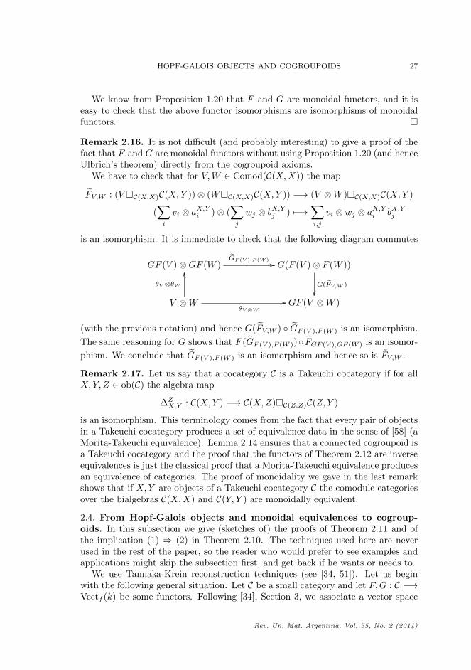
We know from Proposition 1.20 that F and G are monoidal functors, and it iseasy to check that the above functor isomorphisms are isomorphisms of monoidalfunctors.

Remark 2.16. It is not difficult (and probably interesting) to give a proof of thefact that F and G are monoidal functors without using Proposition 1.20 (and henceUlbrich’s theorem) directly from the cogroupoid axioms.

We have to check that for V,W ∈ Comod(C(X,X)) the map

FV,W : (VC(X,X)C(X,Y ))⊗ (WC(X,X)C(X,Y )) −→ (V ⊗W )C(X,X)C(X,Y )

(∑i

vi ⊗ aX,Yi )⊗ (∑j

wj ⊗ bX,Yj ) 7−→∑i,j

vi ⊗ wj ⊗ aX,Yi bX,Yj

is an isomorphism. It is immediate to check that the following diagram commutes

GF (V )⊗GF (W )GF (V ),F (W ) // G(F (V )⊗ F (W ))

G(FV,W )

V ⊗W

θV ⊗θW

OO

θV⊗W

// GF (V ⊗W )

(with the previous notation) and hence G(FV,W ) GF (V ),F (W ) is an isomorphism.

The same reasoning for G shows that F (GF (V ),F (W )) FGF (V ),GF (W ) is an isomor-

phism. We conclude that GF (V ),F (W ) is an isomorphism and hence so is FV,W .

Remark 2.17. Let us say that a cocategory C is a Takeuchi cocategory if for allX,Y, Z ∈ ob(C) the algebra map

∆ZX,Y : C(X,Y ) −→ C(X,Z)C(Z,Z)C(Z, Y )

is an isomorphism. This terminology comes from the fact that every pair of objectsin a Takeuchi cocategory produces a set of equivalence data in the sense of [58] (aMorita-Takeuchi equivalence). Lemma 2.14 ensures that a connected cogroupoid isa Takeuchi cocategory and the proof that the functors of Theorem 2.12 are inverseequivalences is just the classical proof that a Morita-Takeuchi equivalence producesan equivalence of categories. The proof of monoidality we gave in the last remarkshows that if X,Y are objects of a Takeuchi cocategory C the comodule categoriesover the bialgebras C(X,X) and C(Y, Y ) are monoidally equivalent.

2.4. From Hopf-Galois objects and monoidal equivalences to cogroup-oids. In this subsection we give (sketches of) the proofs of Theorem 2.11 and ofthe implication (1) ⇒ (2) in Theorem 2.10. The techniques used here are neverused in the rest of the paper, so the reader who would prefer to see examples andapplications might skip the subsection first, and get back if he wants or needs to.

We use Tannaka-Krein reconstruction techniques (see [34, 51]). Let us beginwith the following general situation. Let C be a small category and let F,G : C −→Vectf (k) be some functors. Following [34], Section 3, we associate a vector space


28 JULIEN BICHON

Hom∨(F,G) to such a pair:

Hom∨(F,G) =⊕

X∈ob(C)

Homk(F (X), G(X))/N ,

where N is the linear subspace of⊕

X∈ob(C) Homk(F (X), G(X)) generated by the

elements G(f) u− u F (f), with f ∈ HomC(X,Y ) and u ∈ Homk(F (Y ), G(X)).The class of an element u ∈ Homk(F (X), G(X)) is denoted by [X,u] in Hom∨(F,G)(note that we have changed the order of the functors in [34]: our Hom∨(F,G) isHom∨(G,F ) in [34]). The vector space Hom∨(F,G) has the following universalproperty.

Lemma 2.18. The vector space Hom∨(F,G) represents the functor

Vectf (k) −→ Vect(k), V 7−→ Nat(G,F ⊗ V ).

More precisely, there exists α• ∈ Nat(G,F ⊗ Hom∨(F,G)) such that the map

Homk(Hom∨(F,G), V ) −→ Nat(G,F ⊗ V )

φ 7−→ (1⊗ φ) α•is a bijection.

Proof. Let X in ob(C) and let e1, . . . , en be a basis of F (X). Define

αX : G(X) −→ F (X)⊗ Hom∨(F,G)

by αX(x) =∑i ei ⊗ [X, e∗i ⊗ x]. It is easily seen that αX does not depend on

the choice of a basis of G(X), and that this procedure defines an element α• ∈Nat(G,F ⊗Hom∨(F,G)). It is not difficult to check that the map in the statementof the lemma is a bijection.

The universal property of Hom∨(F,G) gives, for any functor K : C −→ Vectf (k),a linear map

∆KF,G : Hom∨(F,G) −→ Hom∨(F,K)⊗ Hom∨(K,G)

coassociative in the sense of cocategories. The map ∆KF,G may be described as

follows. Let X ∈ ob(C), let φ ∈ F (X)∗, let x ∈ G(X) and let e1, . . . , en be a basisof K(X). Then

∆KF,G([X,φ⊗ x]) =

n∑i=1

[X,φ⊗ ei]⊗ [X, e∗i ⊗ x].

As a particular case of the previous construction, End∨(F ) := Hom∨(F, F ) is acoalgebra, with counit εX induced by the trace: εX([X,u]) = tr(u) for u ∈Hom(F (X), F (X)).

The previous construction enables one to reconstruct a coalgebra from its cate-gory of finite-dimensional comodules and the forgetful functor: this is the Tannakareconstruction theorem.

Theorem 2.19. Let C be a coalgebra and let ΩC : Comodf (C) −→ Vectf (k) bethe forgetful functor. We have a coalgebra isomorphism End∨(ΩC) ∼= C.



Proof. Consider the natural transformation αC : ΩC −→ ΩC ⊗ C induced by thecoactions of C on its comodules. The universal property of End∨ yields a uniquelinear map f : End∨(ΩC) −→ C such that the following diagram commutes

ΩCα• //

αC ##GGGGGGGGG ΩC ⊗ End∨(ΩC)

1⊗fwwooooooooooo

ΩC ⊗ C

It is easy to see that f is a coalgebra morphism. To prove that f is an isomorphism,we proceed by following [51], Lemma 2.2.1 (for another proof see Section 6 in [34]).Consider, for a vector space V , the linear map

Φ : Homk(C, V ) −→ Nat(ΩC ,ΩC ⊗ V )

φ 7−→ (1⊗ φ) αC .

Let us prove that Φ is bijection. This will define a linear map C −→ End∨(ΩC)which necessarily will be an inverse of f . To construct the inverse of Φ, the keyremark is that if ϕ ∈ Nat(ΩC ,ΩC ⊗ V ) and N , M are two finite-dimensionalsubcomodules of C, then

((ε⊗ 1) ϕN )|N∩M = (ε⊗ 1) ϕN∩M = ((ε⊗ 1) ϕM )|N∩M .

This follows from the naturality of ϕ. This enables to define a (linear) map

Ψ : Nat(ΩC ,ΩC ⊗ V ) −→ Homk(C, V )

by Ψ(ϕ)(x) = (ε ⊗ 1) ϕM (x), ∀x ∈ C, where M is any finite-dimensional subco-module of C containing x.

For φ ∈ Homk(C, V ), x ∈ C and M a finite-dimensional subcomodule of Ccontaining x, we have

φ(x) = φ((1⊗ ε) αCM (x)) = (ε⊗ 1) (1⊗ φ) αCM (x) = Ψ(Φ(φ))(x),

which proves that Ψ Φ = id.Let ϕ ∈ Nat(ΩC ,ΩC ⊗ V ). Let M be a finite-dimensional comodule and let D

be a finite-dimensional subcoalgebra of C such that αC(M) ⊂M ⊗D. Then D isa subcomodule of C. Denote by M0 ⊗D the C-comodule whose coaction is givenby 1 ⊗ ∆. It is clear that αCM : M −→ M0 ⊗ D is a C-comodule map, hence bynaturality of ϕ the following diagram commutes

MϕM //

αCM

M ⊗ V

αCM⊗1

M0 ⊗D

ϕM0⊗D// M0 ⊗D ⊗ V


30 JULIEN BICHON

Any linear map D −→M0⊗D is C-colinear, hence again the naturality of ϕ showsthat ϕM0⊗D = 1⊗ ϕD. Hence we have

Φ Ψ(ϕ)M = (1⊗Ψ(ϕ)) αCM = (1⊗Ψ(ϕ)|D) αCM= (1⊗ ε⊗ 1) (1⊗ ϕD) αCM = (1⊗ ε⊗ 1) (αCM ⊗ 1) ϕM = ϕM ,

and this proves that Φ Ψ = id. We conclude that Φ is an isomorphism.

Now assume that C is a monoidal category and that F,G are monoidal functors.Then Hom∨(F,G) inherits an algebra structure, whose product may be describedby the following formula:

[X,u].[Y, v] = [X ⊗ Y, GX,Y (u⊗ v) F−1X,Y ],

where the isomorphisms FX,Y : F (X)⊗ F (Y ) −→ F (X ⊗ Y ) and GX,Y : G(X)⊗G(Y ) −→ G(X ⊗ Y ) are the constraints of the monoidal functors F and G. The

unit element is [I, G0 F−10 ] where I stands for the monoidal unit of C (that we

indeed have an associative algebra structure heavily depends on the fact that Fand G are monoidal functors). It is not difficult to check that the maps ∆K

F,G and

εF are algebra maps. In particular End∨(F ) is a bialgebra.We summarize the above constructions as follows.

Definition 2.20. Let C be a monoidal category. The cocategory Monk(C) is thecocategory whose objects are the monoidal functors C −→ Vectf (k), withMonk(C)(F,G) = Hom∨(F,G) for F,G ∈ Monk(C), and with structural maps ∆••,•and ε• defined above.

We shall need a monoidal version of Lemma 2.18. If A is an algebra and F,G :C −→ Vectf (k) are monoidal functors, denote by Nat⊗(G,F⊗A) the set of elementsθ ∈ Nat(G,F ⊗A) such that the following diagrams commute for any objects X,Y

G(X ⊗ Y )θX⊗Y // F (X ⊗ Y )⊗A

F−1X,Y // F (X)⊗ F (Y )⊗A

G(X)⊗G(Y )

GX,Y

OO

θX⊗θY // F (X)⊗A⊗ F (Y )⊗A 1⊗τ⊗1// F (X)⊗ F (Y )⊗A⊗A

1⊗1⊗mA

OO

F (I)θI // G(I)⊗A

k

F0

OO

u // A ∼= k ⊗A

G0⊗1

OO

Lemma 2.21. Consider the element α• ∈ Nat(G,F⊗Hom∨(F,G)) of Lemma 2.18.We have α• ∈ Nat⊗(G,F ⊗ Hom∨(F,G)) and we have, for any algebra A, a map

Homk−alg(Hom∨(F,G), A) −→ Nat⊗(G,F ⊗A)

φ 7−→ (1⊗ φ) α•which is a bijection.



Proof. The proof is straightforward.

The bialgebra version of the Tannaka duality theorem is as follows.

Theorem 2.22. Let B be a bialgebra and let ΩB : Comodf (B) −→ Vectf (k) bethe forgetful functor. We have a bialgebra isomorphism End∨(ΩB) ∼= B.

Proof. The natural transformation αB : ΩB −→ ΩB ⊗B induced by the coactionsof B on its comodules is an element in Nat⊗(ΩB ,ΩB ⊗ B), by definition of thetensor product of B-comodules. Hence Lemma 2.21 yields a unique algebra mapmap f : End∨(ΩB) −→ B such that the following diagram commutes

ΩCα• //

αC ##GGGGGGGGG ΩC ⊗ End∨(ΩC)

1⊗fwwooooooooooo

ΩC ⊗ CWe know from the proof of Lemma 2.21 that f is a colagebra isomorphism, andhence is a bialgebra isomorphism.

Assume moreover that C is a rigid monoidal category. This means that everyobject X has a left dual ([34, 36]), i.e. there exists a triplet (X∗, eX , dX) whereX∗ ∈ ob(C), while eX : X∗ ⊗X −→ I (I is the monoidal unit of C) and dX : I −→X ⊗X∗ are morphisms of C such that:

(1X ⊗ eX) (dX ⊗ 1X) = 1X and (eX ⊗ 1X∗) (1X∗ ⊗ dX) = 1X∗ .

The rigidity of C allows one to define a duality endofunctor of C, which will be usedin the proof of the following result, which generalizes [64], using the same idea.

Proposition 2.23. Let C be a rigid monoidal category. Then the cocategoryMonk(C) has a cogroupoid structure.

Proof. We have to construct the linear maps SF,G : Hom∨(F,G) −→ Hom∨(G,F ).We fix for every X ∈ ob(C) a left dual (X∗, eX , dX) (with I∗ = I for the monoidalunit). This defines a contravariant endofunctor of C: X 7−→ X∗, f 7−→ f∗, wherefor f : X −→ Y , the morphism f∗ : Y ∗ −→ X∗ is defined by the composition

Y ∗1⊗dX // Y ∗ ⊗ (X ⊗X∗)

1⊗(f⊗1)// Y ∗ ⊗ (Y ⊗X∗) ∼ // (Y ∗ ⊗ Y )⊗X∗ eY ⊗1 // I ⊗X∗ ∼= X∗.

Let X ∈ ob(C). The unicity of a left dual in a monoidal category yields naturalisomorphisms

λFX : F (X)∗ −→ F (X∗) and λGX : G(X)∗ −→ G(X∗)

such that the following diagrams commute:

F (X)∗ ⊗ F (X)eF (X) //

λFX⊗1F (X)

IF0 // F (I)

F (X∗)⊗ F (X)FX∗,X // F (X∗ ⊗X)

F (eX)

OO


32 JULIEN BICHON

F (X)⊗ F (X)∗

1F (X)⊗λFX

IdF (X)oo F0 // F (I)

F (dX)

F (X)⊗ F (X∗)

FX,X∗ // F (X ⊗X∗)(we have endowed Vectf (k) with its standard duality). Let u ∈ Homk(F (X), G(X)).We put

SF,G([X,u]) = [X∗, λFX u∗ (λGX)−1].

It is easy to see that SF,G is a well defined linear map. Now let φ ∈ F (X)∗, letx ∈ F (X) and let e1, . . . , en be a basis of G(X). Then we have

m (1⊗ SG,F ) ∆GF,F ([X,φ⊗ x])

=

n∑i=1

[X,φ⊗ ei][X∗, λGX (e∗i ⊗ x) (λFX)−1]

=

n∑i=1

[X ⊗X∗, GX,X∗ (1G(X) ⊗ λGX) ((φ⊗ ei)⊗ (x⊗ e∗i ))

(1F (X) ⊗ (λFX)−1) F−1X,X∗ ]

= [X ⊗X∗, GX,X∗ (1G(X) ⊗ λGX) dG(X) (φ⊗ x)

(1F (X) ⊗ (λFX)−1) F−1X,X∗ ]

= [X ⊗X∗, G(dX) G0 (φ⊗ x) (1F (X) ⊗ (λFX)−1) F−1X,X∗ ]

= [I, G0 (φ⊗ x) (1F (X) ⊗ (λFX)−1) F−1X,X∗ F (dX)]

= [I, G0 (φ⊗ x) dF (X) F−10 ] = φ(x)[I, G0 F−1

0 ] = εF ([X,φ⊗ x])1.

Since the elements [X,φ⊗ x] linearly span End∨(F ), we have the commutativity ofthe first diagram. The commutativity of the second diagram is proved similarly.

Definition 2.24. Let H be a Hopf algebra. The fibre functor cogroupoid ofH, denoted Fib(H), is the full subcogroupoid of Monk(Comodf (H)) whose objectsare the fibre functors on Comodf (H).

We have now all the ingredients to prove Theorem 2.11.

Proof of Theorem 2.11. Let H be a Hopf algebra and let A be a left H-Galoisobject. Consider the full subcogroupoid D of Fib(H) whose objects are Ω (theforgetful functor) and ΩA (see Ulbrich’s theorem). Let us check thatD is connected.Let φ : A −→ k be a linear map such that φ(1) = 1. For any X ∈ Comodf (H),the maps 1⊗ φ : XHA→ X define a non-zero element in Nat(ΩA,Ω). Hence byLemma 2.18 we have Hom∨(Ω,ΩA) 6= (0) and the cogroupoid D is connected byProposition 2.15.

For any X ∈ Comodf (H), the inclusions XHA ⊂ X ⊗A define an element

β• ∈ Nat⊗(ΩA,Ω⊗A)



which corresponds by Lemma 2.21 to an algebra map g : Hom∨(Ω,ΩA) −→ A, andwe leave it to the reader to check that the following diagram commutes

Hom∨(Ω,ΩA)g //

∆ΩΩ,ΩA

A

ρ

Hom∨(Ω,Ω)⊗ Hom∨(Ω,ΩA)

f⊗g // H ⊗A

where ρ stands for the coaction of H on A and f is the bialgebra isomorphismof Theorem 2.22. This means that if we endow Hom∨(Ω,ΩA) with the left H-comodule algebra structure transported from the Hopf algebra isomorphism f ,then g is an H-comodule algebra morphism. But Hom∨(Ω,ΩA) is H-Galois sinceit is Hom∨(Ω,Ω)-Galois (Proposition 2.8), and hence by Proposition 1.6 g is anisomorphism. We can now consider the connected cogroupoid D0 with two objectsX,Y and

D0(X,X) = H, D0(X,Y ) = A,

D0(Y,X) = Hom∨(ΩA,Ω), D0(Y, Y ) = Hom∨(ΩA,ΩA).

The structural maps of D0 are transported from the connected cogroupoid D viathe isomorphisms f and g, and we are done.

We get the following result as a corollary of the proof.

Proposition 2.25. Let H be a Hopf algebra. The cogroupoid Fib(H) is connected.

Proof. If A is a left H-Galois object, we have seen in the previous proof thatHom∨(Ω,ΩA) 6= (0). Hence the result follows from Ulbrich’s theorem (any fibrefunctor is isomorphic to some ΩA) and Proposition 2.15.

Proof of Theorem 2.10. LetH, L be some Hopf algebras and let F : Comod(H) −→Comod(L) be a k-linear monoidal equivalence. Then F induces a monoidal equiv-alence Comodf (H) −→ Comodf (L), still denoted F (see Proposition 1.16). It isclear that ΩL F is a fibre functor on Comodf (H). It is not difficult to constructa linear map End∨(ΩL) −→ End∨(ΩL F ) which is a Hopf algebra map since F ismonoidal and is an isomorphism since F is an equivalence. LetD be the (connected)subcogroupoid of Fib(H) whose objects are ΩH and ΩL F . By Theorem 2.22 wehave Hopf algebra isomorphisms End∨(ΩH) ∼= H and End∨(ΩL) ∼= L, and henceEnd∨(ΩL F ) ∼= L. Therefore we get, by transporting the appropriate structuresfrom the connected cogroupoid D, a cogroupoid D0 with two objects X,Y suchthat H = D0(X,X) and L = D0(Y, Y ).

2.5. The weak Hopf algebra of a finite cogroupoid. In this short subsectionwe connect the theory of cogroupoids (and hence of Hopf-Galois objects) with thetheory of weak Hopf algebras [15] (we do not recall here the precise definitionof a weak Hopf algebra). Since cogroupoids are non commutative generalizationsof groupoids, it is natural to wonder if they are linked with weak Hopf algebras,one of the most well-known non commutative generalization of groupoids. Not


34 JULIEN BICHON

surprisingly, the following construction shows that this is indeed the case. The(unpublished) result was obtained in collaboration with Grunspan in 2003-2004.

Proposition 2.26. Let C be a cogroupoid and let X1, . . . , Xn ∈ ob(C). For i, j ∈1, . . . , n, Put C(i, j) = C(Xi, Xj), ∆k

i,j = ∆XkXi,Xj

, Si,j = SXi,Xj , εi = εXi .

Consider the direct sum of algebras

H =

n⊕i,j=1

C(i, j).

Then H has a weak Hopf algebra structure defined as follows.

(1) The comultiplication ∆ : H −→ H ⊗H is defined by

∆(ai,j) =

n∑k=1

∆ki,j(a

i,j) =

n∑k=1

ai,k(1) ⊗ ak,j(2).

(2) The counit ε : H −→ k is defined by ε|C(i,j) = δijεi.(3) The antipode S : H −→ H is defined by S|C(i,j) = Si,j.

The proof is done by a straightforward verification.

Remark 2.27. (1) The use of quantum groupoids (in a different framework)in the study of monoidal equivalences also arose (much earlier) in the workof Bruguieres [16].

(2) It is also worth noting that De Commer [20, 21] obtained independentlymore or less the same result in his investigation of Galois objects for mul-tiplier Hopf algebras and operator algebraic quantum groups.

3. Examples of connected cogroupoids

This section is devoted to the presentation of some examples of connectedcogroupoids. We hope that these examples will convince the reader that veryoften in concrete situations it is easy and natural to work with cogroupoids.

3.1. The bilinear cogroupoid B. Let E ∈ GLn(k). The algebra B(E) is thealgebra presented by generators (aij)1≤i,j≤n subject to the relations

E−1atEa = In = aE−1atE,

where a is the matrix (aij)1≤i,j≤n, at is the transpose matrix and In is the n × nidentity matrix.

It admits a Hopf algebra structure, with comultiplication ∆ defined by

∆(aij) =

n∑k=1

aik ⊗ akj , ε(aij) = δij , S(a) = E−1atE.

This Hopf algebra was introduced by Dubois-Violette and Launer [23] as the quan-tum automorphism group of the non degenerate bilinear form associated to E. Thisterminology comes from the following result.



Proposition 3.1 (Universal property of B(E)).

(1) Consider the vector space V = kn with its canonical basis (ei)1≤i≤n. EndowV with the B(E)-comodule structure defined by α(ei) =

∑nj=1 ej ⊗ aji,

1 ≤ i ≤ n. Then the linear map β : V ⊗V −→ k defined by β(ei⊗ej) = λij,1 ≤ i, j ≤ n, where E = (λij), is a B(E)-comodule morphism.

(2) Let H be a Hopf algebra and let V be a finite-dimensional H-comodule of di-mension n. Let β : V ⊗V −→ k be an H-comodule morphism such that theassociate bilinear form is non-degenerate. Then there exists E ∈ GLn(k)such that V is a B(E)-comodule, that β is a B(E)-comodule morphism,and that there exists a unique Hopf algebra morphism φ : B(E) −→ H with(idV ⊗φ) α = α′, where α and α′ denote the coactions on V of B(E) andH respectively.

Proof. The proof is left as an exercise.

It is not difficult to check that Oq(SL2(k)) = B(Eq), where

Eq =

(0 1−q−1 0

)and hence the Hopf algebras B(E) are generalizations of Oq(SL2(k)).

We now will describe B(E) as part of a cogroupoid. We first need a versioninvolving two matrices, as follows.

Let E ∈ GLm(k) and let F ∈ GLn(k). The algebra B(E,F ) is the universalalgebra with generators aij , 1 ≤ i ≤ m, 1 ≤ j ≤ n, satisfying the relations

F−1atEa = In, aF−1atE = Im.

Of course the generator aij in B(E,F ) should be denoted aE,Fij to express thedependence on E and F , but when there is no confusion and we simply denote itby aij . It is clear that B(E,E) = B(E).

In the following lemma we construct the structural maps that will put the alge-bras B(E,F ) in a cogroupoid framework.

Lemma 3.2. (1) For any E ∈ GLm(k), F ∈ GLn(k), G ∈ GLp(k), thereexists an algebra map

∆GE,F : B(E,F ) −→ B(E,G)⊗ B(G,F )

aij 7−→p∑k=1

aik ⊗ akj

and for any M ∈ GLr(k), the following diagrams commute

B(E,F )∆GE,F−−−−→ B(E,G)⊗ B(G,F )

∆ME,F

y ∆ME,G⊗1

yB(E,M)⊗ B(M,F )

1⊗∆GM,F−−−−−−→ B(E,M)⊗ B(M,G)⊗ B(G,F )


36 JULIEN BICHON

B(E,F )

∆FE,F

id

TTTTTTTTTTTTTTTTT

TTTTTTTTTTTTTTTTT

B(E,F )⊗ B(F, F )1⊗εF // B(E,F )

B(E,F )

∆EE,F

id

TTTTTTTTTTTTTTTTT

TTTTTTTTTTTTTTTTT

B(E,E)⊗ B(E,F )εE⊗1 // B(E,F )

where εE is the counit of B(E).(2) For any E ∈ GLm(k), F ∈ GLn(k), there exists an algebra map

SE,F : B(E,F ) −→ B(F,E)op

a 7−→ E−1atF

such that the following diagrams commute

B(E,E)εE //

∆FE,E

ku // B(E,F )

B(E,F )⊗ B(F,E)1⊗SF,E // B(E,F )⊗ B(E,F )

m

OO

B(E,E)εE //

∆FE,E

ku // B(F,E)

B(E,F )⊗ B(F,E)SE,F⊗1 // B(F,E)⊗ B(F,E)

m

OO

Proof. It is a straightforward verification to construct the announced algebra maps:this is left to the reader. The maps involved in the diagrams of part (1) all arealgebra maps, and hence it is enough to check the commutativity on the generatorsof B(E,F ), which is obvious. For the diagrams of part (2), the commutativityfollows from the verification on the generators of B(E,E) (which is immediatesince E−1atF is inverse to a in B(F,E)) and the fact that ∆••,• and S•,• arealgebra maps.

Hence the lemma ensures that we have a cogroupoid.

Definition 3.3. The cogroupoid B is the cogroupoid defined as follows:

(1) ob(B) = E ∈ GLn(k), n ≥ 1;(2) for E,F ∈ ob(B), the algebra B(E,F ) is the algebra defined above;(3) the structural maps ∆••,•, ε• and S•,• are defined in the previous lemma.

So we have a cogroupoid linking all the Hopf algebras B(E), and the naturalnext question is to study the connectedness of B.



Lemma 3.4. Let E ∈ GLm(k), F ∈ GLn(k) with m,n ≥ 2. Then B(E,F ) 6= (0)if and only if tr(E−1Et) = tr(F−1F t).

Proof. It is left as an exercise to check that if B(E,F ) 6= (0) then tr(E−1Et) =tr(F−1F t). Conversely, assume that tr(E−1Et) = tr(F−1F t). To show thatB(E,F ) 6= (0) we can assume that k is algebraically closed and hence that thereexists q ∈ k∗ such that tr(E−1Et) = −q − q−1 = tr(F−1F t). It is shown in [10],by using the diamond lemma, that B(Eq, F ) 6= (0) and hence by Proposition 2.15we conclude that B(E,F ) 6= (0).

Corollary 3.5. Let λ ∈ k. Consider the full subcogroupoid Bλ of B with objects

ob(Bλ) = E ∈ GLn(k), n ≥ 2, tr(E−1Et) = λ.

Then Bλ is a connected cogroupoid.In particular for E ∈ GLm(k), F ∈ GLn(k) with n,m ≥ 2 and tr(E−1Et) =

tr(F−1F t), then B(E,F ) is a B(E)-B(F )-bi-Galois object and is not cleft if m 6= n.

Proof. It follows from the previous lemma and Proposition 2.8 that B(E,F ) is aB(E)-B(F )-bi-Galois object if tr(E−1Et) = tr(F−1F t). Let us check that it is notcleft if m 6= n. For E ∈ GLm(k), let VE be the m-dimensional B(E)-comodule withbasis vE1 , . . . , v

Em and with B(E)-coaction α(vEi ) =

∑j v

Ej ⊗ aji. Let

Θ : Comod(B(E)) ∼=⊗ Comod(B(F ))

V 7−→ VB(E)B(E,F ),

Θ′ : Comod(B(F )) ∼=⊗ Comod(B(E))

V 7−→ VB(F )B(F,E)

be the inverse monoidal equivalences induced by the bi-Galois objects B(E,F )and B(F,E) (see Theorem 2.12). We shall show that Θ(VE) ∼= VF , which byTheorem 1.17, will prove that B(E,F ) is not a cleft B(E)-Galois object. It is easyto check that the linear map

νF : VF −→ Θ(VE) = VEB(E)B(E,F )

vFj 7−→m∑i=1

vEi ⊗ aE,Fij

is B(F )-colinear. We get a sequence of colinear maps

VFνF−−−−→ Θ(VE)

Θ(νE)−−−−→ ΘΘ′(VF )'−−−−→ VF

whose composition is the identity map, as shown by the following concrete compu-tation

VF −→ VEB(E)B(E,F ) −→(VFB(F )B(F,E)

)B(E)B(E,F ) ∼= VF

vFj 7−→m∑i=1

vEi ⊗ aE,Fij 7−→

m∑i=1

n∑k=1

vFk ⊗ aF,Eki ⊗ a

E,Fij ←− [ vFj


38 JULIEN BICHON

Hence νF is injective, Θ(νE) is surjective, and νF is surjective by the symmetricargument.

Corollary 3.6. Let E ∈ GLn(k) and let q ∈ k∗ be such that tr(E−1Et) = −q−q−1.Then we have a k-linear equivalence of monoidal categories

Comod(B(E)) ∼=⊗ Comod(Oq(SL2(k)).

Proof. This follows from the previous corollary and Corollary 2.9.

This result has a number of interesting consequences in characteristic zero:

(1) ([10]) Any cosemisimple Hopf algebra having a (co-)representation semi-ring isomorphic to the one of O(SL2) is isomorphic to B(E) for some matrixE ∈ GLn(k) (n ≥ 2) such that the solutions of tr(E−1Et) = −q − q−1 aregeneric (i.e. q = ±1 or q is not a root of unity).

(2) ([10]) For E ∈ GLm(k), F ∈ GLn(k), the Hopf algebras B(E) and B(F )are isomorphic if and only if m = n and there exists P ∈ GLn(k) such thatF = PEP t (i.e. the bilinear forms associated to E and F are equivalent,by [50] this is equivalent to say that the matrices E−1Et and F−1F t areconjugate).

(3) ([9]) For any m ≥ 1, there exist cosemisimple Hopf algebras having anantipode of order 2m.

We shall also see in Section 4 that one can deduce easily the classification ofGalois objects over B(E) from these results.

3.2. The universal cosovereign cogroupoid H. We present in this subsectionanother example of cogroupoid involving non cleft Galois objects. This is alsoan occasion to advertize on an interesting but not very well known class of Hopfalgebras.

Let F ∈ GLn(k). The algebra H(F ) [8] is defined to be the universal algebrawith generators (uij)1≤i,j≤n, (vij)1≤i,j≤n and relations:

uvt = vtu = In, vFutF−1 = FutF−1v = In,

where u = (uij), v = (vij) and In is the identity n× n matrix. The algebra H(F )has a Hopf algebra structure defined by

∆(uij) =∑k

uik ⊗ ukj , ∆(vij) =∑k

vik ⊗ vkj ,

ε(uij) = ε(vij) = δij , S(u) = tv, S(v) = F tuF−1.

Furthermore, H(F ) is a cosovereign Hopf algebra (see [8] for the precise meaning):in particular this means that any finite-dimensional H(F )-comodule is isomorphicto its bidual (let us say that a Hopf algebra having this property is coreflexive).The Hopf algebras H(F ) are called the universal cosovereign Hopf algebras in [8]because they have the following universal property.

Proposition 3.7. Let H be a Hopf algebra and let V be a finite dimensional H-comodule isomorphic to its bidual comodule V ∗∗. Then there exists a matrix F ∈GLn(k) (n = dimV ) such that V is an H(F )-comodule and such that there exists



a unique Hopf algebra morphism π : H(F ) −→ H satisfying (1V ⊗ π) βV = αV ,where αV : V −→ V ⊗H and βV : V −→ V ⊗H(F ) denote the coactions of H andH(F ) on V respectively.

VβV //

αV

""FFFF

FFFF

F V ⊗H(F )

1V ⊗f

xxr rr

rr

V ⊗H

In particular, every finitely generated coreflexive Hopf algebra is a homomorphicquotient of some Hopf algebra H(F ).

Proof. Let e1, . . . , en be a basis of V and let xij , 1 ≤ i, j ≤ n be elements of Hsuch that αV (ei) =

∑k ek ⊗ xki, ∀i. Put yij = S(xji). Then we have xyt =

In = ytx for the matrices x = (xij) and y = (yij) since H is a Hopf algebra.Let f : V −→ V ∗∗ be an H-colinear isomorphism, with f(ei) =

∑k λkiek, for

M = (λij) ∈ Mn(k). The H-colinearity of f means that S2(x)M = Mx, i.e.S(y)t = S2(x) = MxM−1. We also have yS(y) = In = S(y)y since H is a Hopf

algebra, so we get yM−1txtM t = In = M−1txtM ty. Hence we get a Hopf algebra

map π : H(M−1t) −→ H such π(uij) = xij and π(vij) = yij . An H(M−1t)-comodule structure on V is defined by letting βV (ei) =

∑k ek⊗uki, and it is clear

that π satisfies the property in the statement, while uniqueness is clear. The lastassertion follows from the previous one and the fact that a Hopf algebra that isfinitely generated as an algebra is generated (as a Hopf algebra) by the coefficientsof one finite-dimensional comodule.

The above universal property indicates that the Hopf algebras H(F ) are thequantum analogues of O(GLn(k)) (as soon as we believe that a finite-dimensionalrepresentation of a quantum group should be isomorphic with its bidual).

Similarly to the previous subsection, we describe H(F ) as part of a cogroupoid,and we begin with a generalization involving two matrices.

Let E ∈ GLm(k) and let F ∈ GLn(k). The algebra H(E,F ) is the algebrapresented by generators uij , vij , 1 ≤ i ≤ m, 1 ≤ j ≤ n, and subject to the relations

uvt = Im = vFutE−1, vtu = In = FutE−1v.

When E = F , we have H(F, F ) = H(F ).The structural morphisms of the corresponding cogroupoid are constructed in

the following lemma.

Lemma 3.8. (1) For any E ∈ GLm(k), F ∈ GLn(k), G ∈ GLp(k), thereexists an algebra map

∆GE,F : H(E,F ) −→ H(E,G)⊗H(G,F )

uij , vij 7−→p∑k=1

uik ⊗ ukj ,p∑k=1

vik ⊗ vkj


40 JULIEN BICHON

and for any M ∈ GLr(k), the following diagrams commute

H(E,F )∆GE,F−−−−→ H(E,G)⊗H(G,F )

∆ME,F

y ∆ME,G⊗1

yH(E,M)⊗H(M,F )

1⊗∆GM,F−−−−−−→ H(E,M)⊗H(M,G)⊗H(G,F )

H(E,F )

∆FE,F

id

TTTTTTTTTTTTTTTTT

TTTTTTTTTTTTTTTTT

H(E,F )⊗H(F, F )1⊗εF // H(E,F )

H(E,F )

∆EE,F

id

TTTTTTTTTTTTTTTTT

TTTTTTTTTTTTTTTTT

H(E,E)⊗H(E,F )εE⊗1 // H(E,F )

(2) For any E ∈ GLm(k), F ∈ GLn(k), there exists an algebra map

SE,F : H(E,F ) −→ H(F,E)op

u, v 7−→ vt, EutF−1


H(E,E)εE //

∆FE,E

ku // H(E,F )

H(E,F )⊗H(F,E)1⊗SF,E // H(E,F )⊗H(E,F )

m

OO

H(E,E)εE //

∆FE,E

ku // H(F,E)

H(E,F )⊗H(F,E)SE,F⊗1 // H(F,E)⊗H(F,E)

m

OO

Proof. The proof is similar to that of Lemma 3.2.

Hence the lemma ensures that we have a cogroupoid.

Definition 3.9. The cogroupoid H is the cogroupoid defined as follows:

(1) ob(H) = F ∈ GLn(k), n ≥ 1;(2) for E,F ∈ ob(H), the algebra H(E,F ) is the algebra defined above;(3) the structural maps ∆••,•, ε• and S•,• are defined in the previous lemma.

So we have a cogroupoid linking all the Hopf algebras H(F ), and the naturalnext question is to study the connectedness of H.



Lemma 3.10. Let E ∈ GLm(k), F ∈ GLn(k) with m,n ≥ 2. Then H(E,F ) 6= (0)if and only if tr(E) = tr(F ) and tr(E−1) = tr(F−1).

Proof. It is left as an exercise to check that if H(E,F ) 6= (0) then tr(E) = tr(F )and tr(E−1) = tr(F−1). The proof of the converse uses the diamond lemma, itmight be found in [12].

Corollary 3.11. Let λ, µ ∈ k. Consider the full subcogroupoid Hλ,µ of H withobjects

ob(Hλ,µ) = F ∈ GLn(k), n ≥ 2, tr(F ) = λ, tr(F−1) = µ.

Then Hλ,µ is a connected cogroupoid.In particular for E ∈ GLm(k), F ∈ GLn(k) with n,m ≥ 2, tr(E) = tr(F ) and

tr(E−1) = tr(F−1), then H(E,F ) is a H(E)-H(F )-bi-Galois object and is not cleftif n 6= m.

Proof. The proof is a copy and paste of the proof of Corollary 3.5.

We can use this result to deduce the corepresentation theory of H(F ) when Fis a generic matrix. Let us introduce some notation and terminology.

• Let F ∈ GLn(k). We say that F is normalized if tr(F ) = tr(F−1). We saythat F is normalizable if there exists λ ∈ k∗ such that tr(λF ) = tr((λF )−1).Over an algebraically closed field, any matrix is normalizable unless tr(F ) =0 6= tr(F−1) or tr(F ) 6= 0 = tr(F−1). The study of the Hopf algebra H(F )for a normalizable matrix reduces to the case when F is normalized, sinceH(λF ) = H(F ).• Let q ∈ k∗. As usual, we say that q is generic if q is not a root of unity

of order N ≥ 3. We say that a matrix F ∈ GLn(k) is generic if F isnormalized and if the solutions of q2 − tr(F )q + 1 = 0 are generic.

• Let q ∈ k∗. We put Fq =

(q−1 00 q

)∈ GL2(k). The Hopf algebra H(Fq)

is denoted by H(q).• Let F ∈ GLn(k). The natural n-dimensional H(F )-comodules associated

to the multiplicative matrices u = (uij) and v = (vij) are denoted by Uand V , with V = U∗.• We will consider the coproduct monoid N ∗ N. Equivalently N ∗ N is the

free monoid on two generators, which we denote, by α and β. There is aunique antimultiplicative morphism − : N ∗ N −→ N ∗ N such that e = e,α = β and β = α (e denotes the unit element of N ∗ N).

The corepresentation theory of H(F ) is described in the following result from[12]. Here k denotes an algebraically closed field.

Theorem 3.12. Let F ∈ GLn(k) (n ≥ 2) be a normalized matrix.(a) Let q ∈ k∗ be such that q2−tr(F )q+1 = 0. Then we have a k-linear equivalenceof monoidal categories

Comod(H(F )) ∼=⊗ Comod(H(q)).


42 JULIEN BICHON

We assume now that k is a characteristic zero field.(b) The Hopf algebra H(F ) is cosemisimple if and only if F is a generic matrix.(c) Assume that F is generic. To any element x ∈ N∗N corresponds a simple H(F )-comodule Ux, with Ue = k, Uα = U and Uβ = V . Any simple H(F )-comodule isisomorphic to one of the Ux, and Ux ∼= Uy if and only if x = y. For x, y ∈ N ∗ N,we have U∗x

∼= Ux and

Ux ⊗ Uy ∼=⊕

a,b,g∈N∗N|x=ag,y=gb

Uab.

Part (a) follows from Corollary 3.11 and Corollary 2.9 and reduces the studyto the case of H(q). One then constructs a Hopf algebra embedding H(q) ⊂k[z, z−1] ∗ Oq(SL2(k)) and uses properties of Oq(SL2(k)) and results on free prod-ucts of cosemisimple Hopf algebras by Wang [67]. See [12] for details. The fusionrule formulas arose first in [4], where another proof of (c), for positive matricesF ∈ GLn(C), might be found.

3.3. The 2-cocycle cogroupoid of a Hopf algebra. We now come back to thefamiliar Hopf-Galois objects obtained from 2-cocycles, discussed on Section 1, andsee how they behave in the cogroupoid framework.

Let H be a Hopf algebra and let σ, τ ∈ Z2(H). The algebra H(σ, τ) is thealgebra having H as underlying vector space and product defined by

x.y = σ(x(1), y(1))τ−1(x(3), y(3))x(2)y(2).

It is straightforward to check that H(σ, τ) is an associative algebra (with the sameunit as H).

In the following lemma we define all the necessary structural maps for the 2-cocycle cogroupoid of H.

Lemma 3.13. (1) Let σ, τ, ω ∈ Z2(H). The map

∆ωσ,τ = ∆ : H(σ, τ) −→ H(σ, ω)⊗H(ω, τ)

x 7−→ x(1) ⊗ x(2)

is an algebra map, and for any α ∈ Z2(H), the following diagram com-mutes:

H(σ, τ)∆ωσ,τ−−−−→ H(σ, ω)⊗H(ω, τ)

∆ασ,τ

y ∆ασ,ω⊗1

yH(σ, α)⊗H(α, τ)

1⊗∆ωα,τ−−−−−→ H(σ, α)⊗H(α, ω)⊗H(ω, τ)

(2) Let σ ∈ Z2(H). The linear map εσ = ε : H(σ, σ) −→ k is an algebra map,and for any τ ∈ Z2(H), the following diagrams commute:

H(σ, τ)

∆τσ,τ

id

TTTTTTTTTTTTTTTTT

TTTTTTTTTTTTTTTTT

H(σ, τ)⊗H(τ, τ)1⊗ετ // H(σ, τ)

H(σ, τ)

∆τσ,τ

id

TTTTTTTTTTTTTTTTT

TTTTTTTTTTTTTTTTT

H(σ, σ)⊗H(σ, τ)εσ⊗1 // H(σ, τ)



(3) Let σ, τ ∈ Z2(H). Consider the linear map

Sσ,τ : H(σ, τ) −→ H(τ, σ)

x 7−→ σ(x(1), S(x(2)))τ−1(S(x(4)), x(5))S(x(3))

The following diagrams commute:

H(σ, σ)εσ //

∆τσ,σ

ku // H(σ, τ)

H(σ, τ)⊗H(τ, σ)1⊗Sτ,σ // H(σ, τ)⊗H(σ, τ)

m

OO

H(σ, σ)εσ //

∆τσ,σ

ku // H(τ, σ)

H(σ, τ)⊗H(τ, σ)Sσ,τ⊗1 // H(τ, σ)⊗H(τ, σ)

m

OO

Proof. Assertions (1) and (2) are obvious. Let x ∈ H. In H(σ, τ), we have

x(1) · Sτ,σ(x(2))

= x(1) ·(τ(x(2), S(x(3)))σ

−1(S(x(5)), x(6))S(x(4)))

= τ(x(4), S(x(5)))σ−1(S(x(9)), x(10))σ(x(1), S(x(8)))τ

−1(x(3), S(x(6)))x(2)S(x(7))

= τ−1 ∗ τ(x(3), S(x(4)))σ−1(S(x(7)), x(8))σ(x(1), S(x(6)))x(2)S(x(5))

= σ−1(S(x(5)), x(6))σ(x(1), S(x(4)))x(2)S(x(3))

= σ(x(1), S(x(2)))σ−1(S(x(3)), x(4)) = ε(x)1,

where the last identity is (a5) from Theorem 1.6 in [18]. This proves the commu-tativity of the first diagram in (3). For the second diagram, we have in H(τ, σ)

Sσ,τ (x(1)) · x(2)

=(σ(x(1), S(x(2)))τ

−1(S(x(4)), x(5))S(x(3)))· x(6)

= σ(x(1), S(x(2)))τ−1(S(x(6)), x(7))τ(S(x(5)), x(8))σ

−1(S(x(3)), x(10))S(x(4))x(9)

= σ(x(1), S(x(2)))τ−1 ∗ τ(S(x(5)), x(6))σ

−1(S(x(3)), x(8))S(x(4))x(7)

= σ(x(1), S(x(2)))σ−1(S(x(3)), x(6))S(x(4))x(5)

= σ(x(1), S(x(2)))σ−1(S(x(3)), x(4)) = ε(x)1,

where again the last identity is (a5) from Theorem 1.6 in [18].

Definition 3.14. Let H be a Hopf algebra. The 2-cocycle cogroupoid of H,denoted H, is the cogroupoid defined as follows:

(1) ob(H) = Z2(H).(2) For σ, τ ∈ Z2(H), the algebra H(σ, τ) is the algebra H(σ, τ) defined above.


44 JULIEN BICHON

(3) The structural maps ∆••,•, ε• and S•,• are the ones defined in the previouslemma.

The Hopf algebra H(σ, σ) is the Hopf algebra Hσ defined by Doi in [18]. Thealgebras σH and Hσ−1 considered in Example 1.3 are the algebras H(σ, 1) andH(1, σ) respectively (where 1 stand for ε ⊗ ε). It follows that H(σ, 1) is an Hσ-H-bi-Galois object and that H(1, σ) is an H-Hσ-bi-Galois object. The associatedmonoidal equivalence

Comod(H) ∼=⊗ Comod(Hσ)

is isomorphic (as a monoidal functor) to the monoidal equivalence whose underlyingfunctor is the identity (recall that H = Hσ as coalgebras) and whose monoidalconstraints is given by the following isomorphisms

V ⊗W ∼= V ⊗Wv ⊗ w 7→ σ−1(v(1), w(1))v(0) ⊗ w(0).

3.4. The multiparametric GLn-cogroupoid. It is in general unpleasant anddifficult to work with explicit cocycles, and the 2-cocycle cogroupoid in the pre-vious subsection is a theoretical tool. In concrete examples, it is much easier towork with explicit algebras (although it is useful to know that a cocycle lies behindthe constructions, e.g. to prove that the algebras are non-zero), and in this subsec-tion we present an example of a full subcogroupoid of the 2-cocycle cogroupoid ofO(GLn(k)).

We say that a matrix p = (pij) ∈Mn(k) is an AST-matrix (after Artin-Schelter-Tate [2]) if pii = 1 and pijpji = 1 for all i and j. The trivial AST-matrix (i.e. pij = 1for all i and j) is denoted by 1. We denote by AST(n) the set of AST matrices ofsize n.

For p ∈ AST(n), the algebra Op(GLn(k)) ([2]) is the algebra presented bygenerators xij , yij , 1 ≤ i, j ≤ n, subject to the following relations (1 ≤ i, j, k, l ≤ n):

xklxij = pkipjlxijxkl, yklyij = pkipjlyijykl, yklxij = pikpljxijykl,n∑k=1

xikyjk = δij =

n∑k=1

xkiykj .

The presentation we have given avoids the use of the quantum determinant. Thealgebra Op(GLn(k)) has a standard Hopf algebra structure, described as follows:

∆(xij) =∑k

xik ⊗ xkj , ∆(yij) =∑k

yik ⊗ ykj ,

ε(xij) = δij = ε(yij), S(xij) = yji, S(yij) = xji.

When p = 1, one gets the usual Hopf algebra O(GLn(k)).



To put Op(GLn(k)) in a cogroupoid framework, we use the following algebras.For p,q ∈ AST(n), the algebra Op,q(GLn(k)) is the algebra presented by genera-tors xij , yij , 1 ≤ i, j ≤ n, subject to the following relations (1 ≤ i, j, k, l ≤ n):

xklxij = pkiqjlxijxkl, yklyij = pkiqjlyijykl, yklxij = pikqljxijykl,n∑k=1

xikyjk = δij =

n∑k=1

xkiykj .

Lemma 3.15. In this lemma we note Op,q = Op,q(GLn(k)).

(1) For any p,q, r ∈ AST(n), there exists an algebra map

∆rp,q : Op,q −→ Op,r ⊗Or,q

xij , yij 7−→n∑k=1

xik ⊗ xkj ,n∑k=1

yik ⊗ ykj

and for any s ∈ AST(n), the following diagrams commute

Op,q

∆rp,q−−−−→ Op,r ⊗Or,q

∆sp,q

y ∆sp,r⊗1

yOp,s ⊗Os,q

1⊗∆rs,q−−−−−→ Op,s ⊗Os,r ⊗Or,q

Op,q

∆qp,q

id

RRRRRRRRRRRRRRRR

RRRRRRRRRRRRRRRR

Op,q ⊗Oq,q1⊗εq // Op,q

Op,q

∆pp,q

id

RRRRRRRRRRRRRRRR

RRRRRRRRRRRRRRRR

Op,p ⊗Op,qεp⊗1 // Op,q

(2) For any p,q ∈ AST(n), there exists an algebra map

Sp,q : Op,q(GLn(k)) −→ Oq,p(GLn(k))op

x, y 7−→ yt, xt


Op,pεp //

∆qp,p

ku // Op,q

Op,q ⊗Oq,p1⊗Sq,p // Op,q ⊗Op,q

m

OO Op,pεp //

∆qp,p

ku // Oq,p

Op,q ⊗Oq,pSp,q⊗1 // Oq,p ⊗Oq,p

m

OO

Proof. Exercise.

The lemma ensures that we have a cogroupoid.

Definition 3.16. The multiparametric GLn-cogroupoid, denoted GLn, is definedas follows:

(1) ob(GLn) = AST(n);(2) for p,q ∈ AST(n), the algebra GLn(p,q) is the algebra Op,q(GLn(k))

defined above;


46 JULIEN BICHON

(3) the structural maps ∆••,•, ε• and S•,• are defined in the previous lemma.

Proposition 3.17. The multiparametric GLn-cogroupoid is connected.

Proof. We know from Proposition 2.15 that it suffices to show thatOp,1(GLn(k)) 6=(0) for any p ∈ AST(n). Consider the algebra kp[t±1

1 , . . . , t±1n ] presented by gener-

ators t1, . . . , tn, t−11 , . . . , t−1

n subject to the relations (1 ≤ i, k ≤ n)

tit−1i = 1 = t−1

i ti, titk = piktkti, t−1i t−1

k = pikt−1k t−1

i , tit−1k = pkit

−1k ti.

It is not difficult to check that kp[t±11 , . . . , t±1

n ] is a non-zero algebra either by usingthe diamond lemma or by showing that it is isomorphic to the twisted group algebrakσ[Zn] for the 2-cocycle considered in [2]. It is straightforward to check that wehave a surjective algebra map

Op,1(GLn(k)) −→ kp[t±11 , . . . , t±1

n ]

xij , yij 7−→ δijti, δijt−1i ,

and hence Op,1(GLn(k)) 6= (0).

Corollary 3.18. For any p ∈ AST(n), we have a k-linear equivalence of monoidalcategories

Comod(Op(GLn(k))) ∼=⊗ Comod(O(GLn(k)).

4. Classifying Hopf-Galois objects: the fibre functor method

In this section we explain how to classify Hopf-Galois objects by using fibrefunctors via Ulbrich’s theorem. The idea is to study how the fibre functor associatedto the Galois object will transform the “fundamental” morphisms of the categoryof comodules.

4.1. Hopf-Galois objects over B(E). Let E ∈ GLm(k) with m ≥ 2. We firststate the classification result for (left) B(E)-Galois objects. We already know fromthe previous section that B(E,F ) is a left B(E)-Galois object if F ∈ GLn(k)satisfies tr(E−1Et) = tr(F−1F t). Let

X0(E) = F ∈ GLn(k), n ≥ 2 | tr(E−1Et) = tr(F−1F t),

and let ∼ be the equivalence relation on X0(E) defined for F,G ∈ X0(E) withF ∈ GLn(k) and G ∈ GLp(k) by

F ∼ G ⇐⇒ [n = p and ∃P ∈ GLn(k) with F = PGP t].

We put X(E) = X0(E)/∼. The following result is stated in [3].

Theorem 4.1. Let E ∈ GLm(k) with m ≥ 2. The map

X0(E) −→ Gal(B(E))

F 7−→ [B(E,F )]

induces a bijection X(E) ' Gal(B(E)).



Of course the meaning of the bracket symbol [ , ] is that we consider the isomor-phism class of the Galois object. The proof of Theorem 4.1 will follow from theforthcoming Propositions 4.2 and 4.3.

Let VE be the m-dimensional B(E)-comodule with basis vE1 , . . . , vEm and with

B(E)-coaction α(vEi ) =∑j v

Ej ⊗ aji. We know that the nondegenerate bilinear

form

βE : VE ⊗ VE 7−→ k, vEi ⊗ vEj 7−→ λij , E = (λij)

is B(E)-colinear and generates Comod(B(E)) as a tensor category (by the universalproperty of B(E)). So to study the fibre functors on Comod(B(E)) we have to studyhow they transform βE . We then deduce informations on the corresponding Galoisobject.

Proposition 4.2. Let A be a left B(E)-Galois object. Then there exists F ∈ X0(E)such that A ∼= B(E,F ) as Galois objects.

Proof. Let ΩA : Comodf (B(E)) 7−→ Vectf (k) be the fibre functor correspondingto A and consider the bilinear map defined by the composition

β′ : ΩA(VE)⊗ ΩA(VE)∼−−−−→ ΩA(VE ⊗ VE)

ΩA(βE)−−−−−→ ΩA(k)∼−−−−→ k∥∥∥ ∥∥∥ ∥∥∥ ∥∥∥

VEB(E)A⊗ VEB(E)A∼−−−−→ (VE ⊗ VE)B(E)A

βE⊗1−−−−→ kB(E)A∼−−−−→ k

Let w1, . . . , wn be a basis of ΩA(VE) (we have n ≥ 2 by Proposition 1.16). Fori ∈ 1, . . . , n, write

wi =

m∑k=1

vEk ⊗ zki

for elements zki ∈ A, 1 ≤ k ≤ m, 1 ≤ i ≤ n. Let F = (µij) ∈ Mn(k) be such thatβ′(wi ⊗ wj) = µij . We have

β′(wi ⊗ wj)1 = β′(

m∑k,l=1

vEk ⊗ zki ⊗ vEl ⊗ zlj)1 =

m∑k,l=1

zkiλklzlj = µij1,

which means that if z = (zki) ∈Mm,n(A), we have

ztEz = F.

We have to check that the matrix F is invertible. We use the fact that β gives adual for VE in the category of B(E)-comodules. For this consider the linear map

δ : k −→ VE ⊗ VE , 1 7−→∑k,l

λ−1kl v

Ek ⊗ vEl , (with E−1 = (λ−1

kl )).

This map is B(E)-colinear (direct verification) and hence we can consider the linearmap δ′ defined by the composition


48 JULIEN BICHON

δ′ : k∼−−−−→ ΩA(k)

ΩA(δ)−−−−→ ΩA(VE ⊗ VE)(ΩAVE,VE

)−1

−−−−−−−−→ ΩA(VE)⊗ ΩA(VE)∥∥∥ ∥∥∥ ∥∥∥ ∥∥∥k

∼−−−−→ kB(E)Aδ⊗1−−−−→ (VE ⊗ VE)B(E)A

∼−−−−→ VEB(E)A⊗ VEB(E)A

We have

δ′(1) =∑i,j

γijwi ⊗ wj =∑k,l

∑i,j

γijvEk ⊗ zki ⊗ vEl ⊗ vlj ⊗ zlj

for G = (γij) ∈Mn(k) and hence

ΩAVE ,VE δ′(1) =

∑k,l

vEk ⊗ vEl ⊗ (∑i,j

zkiγijzlj).

On the other hand

ΩAVE ,VE δ′(1) =

∑k,l

vEk ⊗ vEl ⊗ λ−1kl 1,

which shows that zGzt = E−1. We have

(1⊗ βE) (δ ⊗ 1) = 1VE

in the monoidal category of B(E)-comodules, so the monoidal functor ΩA trans-forms this equation into

(1⊗ β′) (δ′ ⊗ 1) = 1ΩA(VE).

This means that FG = In, so that F is invertible with G = F−1. We haveztEz = F and zGzt = E−1, hence

F−1ztEz = In and zF−1ztE = Im.

Thus there exists a unique algebra morphism f : B(E,F ) −→ A defined by f(aki) =zki. Moreover it is easy to see that f is left B(E)-colinear since

wi =∑k

vEk ⊗ zki ∈ VEB(E)A.

We conclude by Proposition 1.6 that f is an isomorphism.

To classify the Galois objects B(E,F ) up to isomorphism, it is also useful toexamine the associated fibre functors.

Proposition 4.3. Let F,G ∈ X0(E) with F ∈ GLn(k) and G ∈ GLp(k). Thefollowing assertions are equivalent.

(1) The left B(E)-comodule algebras B(E,F ) and B(E,G) are isomorphic.(2) F ∼ G, i.e. n = p and ∃P ∈ GLn(k) with F = PGP t.



Proof. We use the notation in the previous proof. Let f : B(E,F ) −→ B(E,G) bea left B(E)-comodule algebra isomorphism. Then f induces a linear isomorphism

1⊗ f : VEB(E)B(E,F ) −→ VEB(E)B(E,G).

By Corollary 3.5 and its proof we have n = p and the elements

wi =∑k

vEk ⊗ aE,Fki , w′i =

∑k

vEk ⊗ aE,Gki , 1 ≤ i ≤ n

form respective bases of VEB(E)B(E,F ) and VEB(E)B(E,G). Then there existsM = (mij) ∈ GLn(k) such that 1⊗ f(wi) =

∑jmjiw

′j , ∀i, and hence∑

k

vEk ⊗ f(aE,Fki ) =∑k

vEk ⊗ (∑j

aE,Gkj mji),

which in matrix form gives f(aE,F ) = aE,GM or dropping the exponents f(a) =aM . We have F−1atEa = In in B(E,F ), hence

In = f(F−1atEa) = F−1M tatEaM ⇒MF−1M tatEa = In in B(E,G).

But we have aG−1atE = Im so MF−1M tatE = G−1atE ⇒MF−1M tat = G−1at

and we conclude by multiplying on the right by EaG−1 that MF−1M t = G−1.This proves that F ∼ G.

Conversely, if n = p and ∃P ∈ GLn(k) such that F = PGP t, it is not difficultto show that there exists a unique algebra map f : B(E,F ) −→ B(E,G) such thatf(a) = aP t, that f is an isomorphism and is B(E)-colinear.

Remark 4.4. There is an interesting equivalence relation on Galois objects, calledhomotopy, introduced by Kassel and further developped by Kassel and Schneiderin [38]. The classification of Galois objects over B(E) up to homotopy is studiedin [3].

4.2. Hopf-Galois objects over H(F ). We provide now the classification of theGalois objects over the universal cosovereign Hopf algebras H(F ), following thesame line as the one of the previous subsection.

Let E ∈ GLm(k) with m ≥ 2. We know from the previous section that H(E,F )is a left H(E)-Galois object if F ∈ GLn(k) satisfies tr(E) = tr(F ) and tr(E−1) =tr(F−1). Let

X0(E) = F ∈ GLn(k), n ≥ 2 | tr(E) = tr(F ), tr(E−1) = tr(F−1)and let ≈ be the equivalence relation on X0(E) defined for F,G ∈ X0(E) withF ∈ GLn(k) and G ∈ GLp(k) by

F ≈ G ⇐⇒ [n = p and ∃P ∈ GLn(k) with F = PGP−1].

We put X(E) = X0(E)/≈.

Theorem 4.5. Let E ∈ GLm(k) with m ≥ 2. The map

X0(E) −→ Gal(H(E))

F 7−→ [H(E,F )]

induces a bijection X(E) ' Gal(H(E)).


50 JULIEN BICHON

Theorem 4.5 follows from the forthcoming Propositions 4.6 and 4.7.

Proposition 4.6. Let A be a left H(E)-Galois object. Then there exists F ∈X0(E) such that A ∼= H(E,F ) as Galois objects.

Proof. The reasoning is similar to the one of Proposition 4.2 so we give less detail.Let UE be the m-dimensional H(E)-comodule with basis uE1 , . . . , u

Em and with

H(E)-coaction given by α(uEi ) =∑j u

Ej ⊗ uji. The coaction of the dual comodule

U∗E is given by α∗(uE∗i ) =∑j u

E∗j ⊗ vji. The following linear maps

e : U∗E ⊗ UE −→ k, u∗i ⊗ uj 7−→ δij ,

d : k −→ UE ⊗ U∗E , 1 7−→m∑i=1

ui ⊗ u∗i ,

ε : UE ⊗ U∗E −→ k, ui ⊗ u∗j 7−→ λ−1ij ,

δ : k −→ U∗E ⊗ UE , 1 7−→m∑

i,j=1

λiju∗i ⊗ uj ,

where E = (λij) and E−1 = (λ−1ij ), are H(E)-colinear. Let ΩA : Comodf (H(E))

7−→ Vectf (k) be the fibre functor corresponding to A. Consider the linear mapsdefined by the compositions

e′ : ΩA(U∗E)⊗ ΩA(UE)∼−−−−→ ΩA(U∗E ⊗ UE)

ΩA(e)−−−−→ ΩA(k)∼−−−−→ k∥∥∥ ∥∥∥ ∥∥∥ ∥∥∥

U∗EH(E)A⊗ UEH(E)A∼−−−−→ (U∗E ⊗ UE)H(E)A

e⊗1−−−−→ kH(E)A∼−−−−→ k

d′ : k∼−−−−→ ΩA(k)

ΩA(d)−−−−→ ΩA(UE ⊗ U∗E)(ΩAUE,U∗E

)−1

−−−−−−−−→ ΩA(UE)⊗ ΩA(U∗E)∥∥∥ ∥∥∥ ∥∥∥ ∥∥∥k

∼−−−−→ kH(E)Ad⊗1−−−−→ (UE ⊗ U∗E)H(E)A

∼−−−−→ UEH(E)A⊗ U∗EH(E)A

Then (ΩA(U∗E), e′, d′) is a left dual for ΩA(UE) since ΩA is a monoidal functor.Hence there exist bases w1, . . . , wn and w′1, . . . , w

′n of ΩA(UE) and ΩA(U∗E) respec-

tively (n = dim ΩA(UE) ≥ 2) such that e′(w′i ⊗ wj) = δij and d′(1) =∑i wi ⊗ w′i.

Now write wi =∑k u

Ek ⊗ zki and w′i =

∑k u

E∗k ⊗ cki for elements zki, cki ∈ A.

Then we see that ctz = In and zct = Im.Consider now the linear maps defined by the compositions

ε′ : ΩA(UE)⊗ ΩA(U∗E)∼−−−−→ ΩA(UE ⊗ U∗E)

ΩA(ε)−−−−→ ΩA(k)∼−−−−→ k∥∥∥ ∥∥∥ ∥∥∥ ∥∥∥

UEH(E)A⊗ U∗EH(E)A∼−−−−→ (UE ⊗ U∗E)H(E)A

ε⊗1−−−−→ kH(E)A∼−−−−→ k



δ′ : k∼−−−−→ ΩA(k)

ΩA(δ)−−−−→ ΩA(U∗E ⊗ UE)(ΩAU∗

E,UE

)−1

−−−−−−−−→ ΩA(U∗E)⊗ ΩA(UE)∥∥∥ ∥∥∥ ∥∥∥ ∥∥∥k

∼−−−−→ kH(E)Aδ⊗1−−−−→ (U∗E ⊗ UE)H(E)A

∼−−−−→ U∗EH(E)A⊗ UEH(E)A

Since (ΩA(UE), ε′, δ′) is a left dual for ΩA(U∗E), there exists M = (mij) ∈ GLn(k)

such that ε′(wi ⊗ w′j) = mij and δ′(1) =∑ni,j=1m

−1ij w

′i ⊗ wj . From this we

see that M = ztE−1c and E = cM−1zt. Hence there exists an algebra mapf : H(E,M−1) −→ A such that f(uki) = zki and f(vki) = cki, which is H(E)-colinear, and is an isomorphism by Proposition 1.6.

Proposition 4.7. Let F,G ∈ X0(E) with F ∈ GLn(k) and G ∈ GLp(k). Thefollowing assertions are equivalent.

(1) The left H(E)-comodule algebras H(E,F ) and H(E,G) are isomorphic.(2) F ≈ G, i.e. n = p and ∃P ∈ GLn(k) with F = PGP−1.

Proof. The proof is similar to that of Proposition 4.3: if f : H(E,F ) −→ H(E,G)is a left H(E)-comodule algebra isomorphism, then n = p and there exists M ∈GLn(k) such that f(u) = uM and f(v) = vM t−1

, and then we haveG = M t−1

FM t,so F ≈ G. Conversely, if there exists P ∈ GLn(k) with F = PGP−1, one defines aleft H(E)-comodule algebra isomorphism f : H(E,F ) −→ H(E,G) by f(u) = uP t

and f(v) = vP t−1

.

4.3. Some remarks.

(1) The problem of classifying the fibre functors (or Galois objects) on a comod-ule category is a particular case of the problem of classifying the modulecategories over the comodule category (see [48]), considered for Oq(SL2(k))by Etingof and Ostrik ([25] and [49]). Recent nice contributions on theproblem of classifying module categories (and hence Hopf-Galois objects)were done by Mombelli [44, 45], see also [26].

(2) As we have seen the fibre functor method provides a powerful methodfor classifying Hopf-Galois objects, as least if the comodule category isgenerated by a few equationnaly well defined morphisms. It does not seemto work so well for pointed Hopf algebras, or at least I could not makeit work well. The best technique for pointed Hopf algebras has been fora long time the one by Masuoka [42], but recently new techniques haveemerged, by Masuoka again [43] or more interestingly yet by the alreadymentionned work of Mombelli [44, 45]. Hopf-Galois techniques are useful inthe classification problem for pointed Hopf algebras, in particular to obtainliftings of Nichols algebras, see e.g. the recent paper [1].

5. Applications to comodule algebras

In this section we present applications of bi-Galois theory to the study of comod-ule algebras. The basic result is the following one.


52 JULIEN BICHON

Theorem 5.1. Let H, L be Hopf algebras with a k-linear monoidal equivalence

F : Comod(H) ∼=⊗ Comod(L).

Then F induces an equivalence of categories between right H-comodule algebras andright L-comodule algebras. If B is a right H-comodule algebra, the above monoidalequivalence induces an algebra isomorphism between the respective coinvariant sub-algebras BcoH ∼= F (B)coL.

Proof. A right H-comodule algebra is exactly an algebra in the monoidal cate-gory of right H-comodules, thus the above functor induces the announced categoryequivalence. Let B be a right H-comodule algebra. We have an algebra isomor-phism

HomH(k,B) −→ BcoH

f 7−→ f(1)

where the algebra structure on HomH(k,B) is given by f · g = mB (f ⊗ g). Theabove monoidal functor induces an algebra isomorphism

HomH(k,B) ∼= HomL(F (k), F (B)) ∼= HomL(k, F (B))

and hence induces an algebra isomorphism BcoH ∼= F (B)coL.

The cogroupoid picture might be useful to determine exactly the algebras F (B)and F (B)coL (with F (B) = BHA and F (B)coL = (BHA)coL for an H-L-bi-Galois object A), for example to get a presentation by generators and relation fromthe ones of B and BcoH . We present some illustrations.

5.1. A model comodule algebra for B(E). We continue the study of B(E)-comodules by providing explicit models for the simple B(E)-comodules in thecosemisimple case. We assume that k has characteristic zero in this subsection.

Definition 5.2. Let H be a cosemisimple Hopf algebra. A model H-comodulealgebra is a right H-comodule algebra in which every simple H-comodule appearswith multiplicity one.

It is well known that if q is not a root of unity of order ≥ 3, then the quantumplane algebra kq[x, y] is a model Oq(SL2(k))-comodule algebra, since the degreegrading provides a decomposition

kq[x, y] =⊕n∈N

kq[x, y]n

and the comodules kq[x, y]n, n ∈ N, provide a complete list of simple Oq(SL2(k))-comodules (see e.g. [39]). It is clear from Theorem 5.1 that the property of having amodel comodule algebra is monoidally invariant and hence B(E) will have a modelcomodule algebra when it is cosemisimple.

Definition 5.3. Let M = (αij) ∈ Mm(k) and t ∈ k. The algebra AM,t is thealgebra presented by generators x1, . . . , xm subject to the relation

∑mi,j=1 αijxixj =

t.



When

M = E−1q =

(0 −q1 0

)the algebra AM,0 is the quantum plane kq[x, y], while that algebra AM,1 is thequantum Weyl algebra Aq1(k).

Proposition 5.4. Let E ∈ GLm(k). Then AE−1,t has a right B(E)-comodulealgebra structure defined by the formula

α(xi) =

m∑k=1

xk ⊗ aki.

Let F ∈ GLn(k) be such that tr(E−1Et) = tr(F−1F t) (m,n ≥ 2) and considerthe monoidal equivalence Θ : Comod(B(E)) −→ Comod(B(F )) induced by theB(E)-B(F )-bi-Galois object B(E,F ). We have an isomorphism of B(F )-comodulealgebras Θ(AE−1,t) ∼= AF−1,t.

Proof. It is straightforward to check that AE−1,t has a B(E)-comodule algebrastructure given by the above formula. We give two sketches of proof thatΘ(AE−1,t) ∼= AF−1,t. In the first proof we proceed very similarly to the proofof Corollary 3.5 when we showed that Θ(VE) ∼= VF . It is straightforward to checkthat one has an algebra map

ιF : AF−1,t −→ AE−1,tB(E)B(E,F ) = Θ(AE−1,t)

xFi 7−→m∑k=1

xEk ⊗ aE,Fki

which is B(F )-colinear and the argument of the proof of Corollary 3.5 to show thatιF is an isomorphism works without any change.

A second sketch of proof is as follows [41]. Consider the tensor algebra T (VE) =⊕l∈N V

⊗lE . This is a B(E)-comodule algebra and we have Θ(T (VE)) ∼= T (Θ(VE)) ∼=

T (VF ) as B(F )-comodule algebras. As in the proof of Proposition 4.2, consider theB(E)-colinear map

δE : k −→ VE ⊗ VE , 1 7−→∑k,l

λ−1kl v

Ek ⊗ vEl , (with E−1 = (λ−1

kl )).

By construction AE−1,t = T (VE)/〈δE − t1〉 an with an obvious abuse of notationwe have Θ(δE) = δF (check this) and hence

Θ(AE−1,t) = Θ(T (VE)/〈δE − t1〉) ∼= T (VF )/〈Θ(δE − t1)〉)= T (VF )/〈δF − t1〉 = AF−1,t .

This concludes the proof.

Corollary 5.5. Let E ∈ GLn(k) be such that there exists q ∈ k∗ with tr(E−1Et) =−q − q−1 and q is not a root of unity of order ≥ 3. Then for t ∈ 0, 1, AE−1,t isa model B(E)-comodule algebra.


54 JULIEN BICHON

Proof. The proof follows from Corollary 3.6, the previous proposition and the factthat AE−1

q ,0 = kq[x, y] and AE−1q ,1 = Aq1(k) are model Oq(SL2(k))-comodule alge-

bras (that Aq1(k) is a model Oq(SL2(k))-comodule algebra can be deduced from thefact that kq[x, y] is the graded algebra associated to the natural degree filtrationon Aq1(k)).

Remark 5.6. It follows from the previous results that if B(E) is cosemisimple, thesimple B(E)-comodule corresponding to n ∈ N is the subspace of degree n elementsin AE−1,0.

5.2. An application to invariant theory. The considerations at the beginningof the section allow us to get nice theorems in invariant theory almost for free. Weprovide an illustration taken from [7].

The first and most well-known theorem in invariant theory is the structure the-orem for the algebra of symmetric polynomials. So each time we have a 2-cocycledeformation of O(Sn) (the algebra of functions on the symmetric group Sn), wecan derive a twisted version of the classical theorem on symmetric polynomials.

We begin by introducing some notation. We assume that char(k) 6= 2. Letn ≥ 2. For i ∈ 1, . . . , 2n, we put

i′ = i− 1 and i∗ = i/2, if i is even,

i′ = i+ 1 and i∗ = i′/2, if i is odd.

We have i′∗ = i∗. Let AST2(n) be the set of AST matrices p = (pij) ∈Mn(k) withpii = 1 and pij = pji = ±1 for any i and j.

For p ∈ AST2(n), the algebra Op(S2n) is the algebra presented by generators(xij)1≤i,j≤2n and subject to the relations (1 ≤ i, j, k, l ≤ 2n):

xijxik = δjkxij , xjixki = δjkxji,

2n∑l=1

xil = 1 =

2n∑l=1

xli,

(3 + pi∗j∗)xkjxli + (1− pi∗j∗)xkjxli′ + (1− pi∗j∗)xkj′xli + (pi∗j∗ − 1)xkj′xli′

= (3 + pl∗k∗)xlixkj + (1− pl∗k∗)xl′ixkj + (1− pl∗k∗)xlixk′j + (pl∗k∗ − 1)xl′ixk′j .

If p = 1 then O1(S2n) is just the algebra of functions on S2n (see [68]). It is adirect verification to check that Op(S2n) is a Hopf algebra with

∆(xij) =∑k

xik ⊗ xkj , ε(xij) = δij , S(xij) = xji.

We consider the algebra kp[x1, . . . , x2n] presented by generators x1, . . . , x2n subjectto the relations

4xixj = (3 + pi∗j∗)xjxi + (1− pi∗j∗)xj′xi + (1− pi∗j∗)xjxi′ + (pi∗j∗ − 1)xj′xi′ .

It is clear that k1[x1, . . . , x2n] = k[x1, . . . , x2n].Our aim is to prove the following result.



Theorem 5.7. The algebra kp[x1, . . . , x2n] has a right Op(S2n)-comodule alge-bra structure defined by δ(xi) =

∑k xk ⊗ xki, and the algebra of coinvariants

kp[x1, . . . , x2n]coOp(S2n) is a (commutative) algebra of polynomials on 2n variables.

The strategy is clear: we have to construct a k-linear monoidal equivalence

Comod(O(S2n)) ∼=⊗ Comod(Op(S2n))

sending k[x1, . . . , x2n] to kp[x1, . . . , x2n], and combine the classical theorem onsymmetric polynomials with Theorem 5.1. In order to do this we construct anappropriate connected cogroupoid.

Let p,q ∈ AST2(n). The algebra Op,q(S2n) is the algebra presented by gener-ators (xij)1≤i,j≤2n subject to the relations:

xijxik = δjkxij , xjixki = δjkxji,

2n∑l=1

xil = 1 =

2n∑l=1

xli,

(3 + qi∗j∗)xkjxli + (1− qi∗j∗)xkjxli′ + (1− qi∗j∗)xkj′xli + (qi∗j∗ − 1)xkj′xli′

= (3 + pl∗k∗)xlixkj + (1− pl∗k∗)xl′ixkj + (1− pl∗k∗)xlixk′j + (pl∗k∗ − 1)xl′ixk′j .

Lemma 5.8. In this lemma we note Op,q = Op,q(S2n).

(1) For any p,q, r ∈ AST2(n), there exists an algebra map

∆rp,q : Op,q −→ Op,r ⊗Or,q

xij 7−→n∑k=1

xik ⊗ xkj ,

and for any s ∈ AST2(n), the following diagrams commute

Op,q

∆rp,q−−−−→ Op,r ⊗Or,q

∆sp,q

y ∆sp,r⊗1

yOp,s ⊗Os,q

1⊗∆rs,q−−−−−→ Op,s ⊗Os,r ⊗Or,q

Op,q

∆qp,q

id

RRRRRRRRRRRRRRRR

RRRRRRRRRRRRRRRR

Op,q ⊗Oq,q1⊗εq // Op,q

Op,q

∆pp,q

id

RRRRRRRRRRRRRRRR

RRRRRRRRRRRRRRRR

Op,p ⊗Op,qεp⊗1 // Op,q

(2) For any p,q ∈ AST(n), there exists an algebra map

Sp,q : Op,q(S2n) −→ Oq,p(S2n)op

x 7−→ xt


56 JULIEN BICHON


Op,pεp //

∆qp,p

ku // Op,q

Op,q ⊗Oq,p1⊗Sq,p // Op,q ⊗Op,q

m

OO Op,pεp //

∆qp,p

ku // Oq,p

Op,q ⊗Oq,pSp,q⊗1 // Oq,p ⊗Oq,p

m

OO

Proof. This is a straightforward verification. One way to simplify the computationsis as follows. For i, j, l, k ∈ 1, . . . , 2n and p ∈ ASR2(n), put

Rklij (p) = δi∗l∗δj∗k∗(1 + (−1)i−l + (−1)j−k + (−1)i−l+j−kpj∗i∗

).

With this notation, the second relations defining Op,q are∑α,β

Rklαβ(p)xαixβj =∑α,β

Rαβij (q)xkαxlβ .

With this compact notation the verification that ∆rp,q is well-defined is easy.

The lemma ensures that we have a cogroupoid whose objects are the elementsof AST2(n) and whose algebras are the above algebras Op,q(S2n). The followinglemma and Proposition 2.15 ensure that the cogroupoid is connected, and hencethat each Op,q(S2n) is an Op(S2n)-Oq(S2n)-bi-Galois object.

Lemma 5.9. We have Op,1(S2n) 6= (0) for any p ∈ AST2(n).

Proof. Consider the algebra A presented by generators t1, . . . , tn subject to therelations t2i = 1, ∀i, titj = pijtjti. It is not difficult to check that A is a non-zero algebra (it is isomorphic with the twisted group algebra kσ[(Z/2Z)n] for anappropriate 2-cocycle). One then checks that there exists an algebra map

Op,1(S2n) −→ A

xij 7−→δi∗,j∗

2(1 + (−1)j−iti∗)

and hence Op,1(S2n) is a non-zero algebra.

Proof of Theorem 5.7. The existence of the announced Op(S2n)-comodule algebrastructure on kp[x1, . . . , x2n] is left to the reader. Also the reader will check theexistence of an algebra map

kp[x1, . . . , x2n] −→ kq[x1, . . . , xn]Oq(S2n)Oq,p(S2n)

xi 7−→n∑k=1

xk ⊗ xki

for any p,q ∈ AST2(n). From this he will check, using the technique alreadyused several times (e.g. in the proof of Corollary 3.5), that the monoidal equiva-lence associated to the Oq(S2n)-Op(S2n)-bi-Galois object Oq,p(S2n) transforms thealgebra kq[x1, . . . , xn] into the algebra kp[x1, . . . , xn]. Theorem 5.1 and the classi-cal theorem on the structure of symmetric polynomials (the algebra of symmetric



polynomials is a polynomial algebra on the elementary symmetric polynomialss1, . . . , s2n) conclude the proof.

6. Yetter-Drinfeld modules

In this section the previous results and constructions are applied to Yetter-Drinfeld modules. We give an application to Brauer groups of Hopf algebras, whilean application to bialgebra cohomology will be given at the end of the next Section.

Let H be a Hopf algebra. Recall that a (right-right) Yetter-Drinfeld moduleover H is a right H-comodule and right H-module V satisfying the condition

(v ← x)(0) ⊗ (v ← x)(1) = v(0) ← x(2) ⊗ S(x(1))v(1)x(3).

The category of Yetter-Drinfeld modules over H is denoted YDHH : the morphismsare the H-linear H-colinear maps. Endowed with the usual tensor product ofmodules and comodules, it is a monoidal category.

6.1. Monoidal equivalence between categories of Yetter-Drinfeld mod-ules. Recently some authors ([17, 5]) have used the fact that the Yetter-Drinfeldcategories of Hopf algebras that are cocycle deformation of each other are monoidallyequivalent. This result is a particular case of the following result.

Theorem 6.1. Let H and L be two Hopf algebras such that there exists a k-linearmonoidal equivalence between Comod(H) and Comod(L). Then there exists a k-

linear monoidal equivalence between YDHH and YDLL.

A sketch of a quick proof of the theorem is as follows: the weak center (seethe appendix in [54]) of the category Comod(H) is monoidally equivalent with

the category YDHH , and hence a monoidal equivalence between Comod(H) and

Comod(L) will induce a monoidal equivalence between YDHH and YDLL.

The result that the weak center of Comod(H) is YDHH is stated in [54]. It isprobably well-known to many specialists, but to the best of my knowledge no com-plete proof is avalaible in the literarure (although it is similar to the more familiarmodule case). Hence it might be useful to have a direct and more constructive proofusing bi-Galois objects and cogroupoids. It is the aim of the section to provide sucha proof.

Proposition 6.2. Let C be cogroupoid, let X,Y ∈ ob(C) and let V be a rightC(X,X)-module.

(1) V ⊗ C(X,Y ) has a right C(Y, Y )-module structure defined by(v ⊗ aX,Y

)← bY,Y = v ← bX,X(2) ⊗ SY,X(bY,X(1) )aX,Y bX,Y(3) .

Endowed with the right C(Y, Y )-comodule structure defined by 1 ⊗ ∆YX,Y ,

V ⊗ C(X,Y ) is a Yetter-Drinfeld module over C(Y, Y ).(2) If moreover V is Yetter-Drinfeld module, then VC(X,X)C(X,Y ) is Yetter-

Drinfeld submodule of V ⊗ C(X,Y ).

Note that when V = k is the trivial comodule, then the action of C(Y, Y ) onC(X,Y ) is the Miyashita-Ulbrich action (see [54], Definition 2.1.8).


58 JULIEN BICHON

Proof. We freely use Proposition 2.13. Let us first check that the above formuladefines a right C(Y, Y )-module structure on V ⊗ C(X,Y ). It is clear that (v ⊗aX,Y )← 1Y,Y = v ⊗ aX,Y . We have

(v ⊗ aX,Y )← (bY,Y cY,Y ) = v ← (bX,X(2) cX,X(2) )⊗ SY,X(bY,X(1) cY,X(1) )aX,Y bX,Y(3) cX,Y(3)

= (v ← bX,X(2) )← cX,X(2)

⊗ SY,X(cY,X(1) )SY,X(bY,X(1) )aX,Y bX,Y(3) cX,Y(3)

=(v ← bX,X(2) ⊗ SY,X(bY,X(1) )aX,Y bX,Y(3)

)← cX,X

=(v ⊗ aX,Y ← bY,Y

)← cY,Y ,

and hence V ⊗ C(X,Y ) is a right C(Y, Y )-module. We also have

((v ⊗ aX,Y )← bY,Y )(0) ⊗ ((v ⊗ aX,Y )← bY,Y )(1)

= v ← bX,X(2) ⊗∆YX,Y (SY,X(bY,X(1) )aX,Y bX,Y(3) )

= v ← bX,X(3) ⊗ SY,X(bY,X(2) )aX,Y(1) bX,Y(4) ⊗ SY,Y (bY,Y(1) )aY,Y(2) bY,Y(5)

= ((v ⊗ aX,Y(1) )← bY,Y(2) )⊗ SY,Y (bY,Y(1) )aY,Y(2) bY,Y(3)

= (v ⊗ aX,Y )(0) ← bY,Y(2) ⊗ SY,Y (bY,Y(1) )(v ⊗ aX,Y )(1)bY,Y(3) ,

and this shows that V ⊗ C(X,Y ) is a Yetter-Drindeld module over C(Y, Y ).Assume now that V is a Yetter-Drinfeld module and let us check that

VC(X,X)C(X,Y ) is Yetter-Drinfeld submodule of V ⊗C(X,Y ). We already know

that it is a subcomodule. Let∑i vi ⊗ a

X,Yi ∈ VC(X,X)C(X,Y ). We must check

that

(∑i

vi⊗aX,Yi )← bY,Y =∑i

vi ← bX,X(2) ⊗SY,X(bY,X(1) )aX,Yi bX,Y(3) ∈ VC(X,X)C(X,Y ).

We have∑i

(vi ← bX,X(2) )(0) ⊗ (vi ← bX,X(2) )(1) ⊗ SY,X(bY,X(1) )aX,Yi bX,Y(3)

=∑i

vi(0) ← bX,X(3) ⊗ SX,X(bX,X(2) )vi(1)bX,X(4) ⊗ SY,X(bY,X(1) )aX,Yi bX,Y(5)

=∑i

vi ← bX,X(3) ⊗ SX,X(bX,X(2) )aX,Xi(1) bX,X(4) ⊗ SY,X(bY,X(1) )aX,Yi(2) b

X,Y(5)

=∑i

vi ← bX,X(2) ⊗∆XX,Y (SY,X(bY,X(1) )aX,Yi bX,Y(3) ),

which gives the result.

Theorem 6.3. Let C be a connected cogroupoid. Then for any X,Y ∈ ob(C), thefunctor

YDC(X,X)C(X,X) −→ YD

C(Y,Y )C(Y,Y )

V 7−→ VC(X,X)C(X,Y )



is an equivalence of k-linear monoidal categories.

Proof. First we have to check that we indeed have a functor, i.e. that if f : V −→Wis a morphism of Yetter-Drinfeld modules, then f ⊗ 1 : VC(X,X)C(X,Y ) −→WC(X,X)C(X,Y ) is a morphism of Yetter-Drindeld modules. We already know itis colinear, and it is not difficult to check that it is also C(Y, Y )-linear. Hence wehave our functor

F : YDC(X,X)C(X,X) −→ YD

C(Y,Y )C(Y,Y )

V 7−→ VC(X,X)C(X,Y ).

Consider the symmetrically defined functor

G : YDC(Y,Y )C(Y,Y ) −→ YD

C(X,X)C(X,X)

V 7−→ VC(Y,Y )C(Y,X).

We know from Theorem 2.12 and its proof that these are inverse equivalences oncomodules and hence we have to check that the comodule isomorphisms G F ∼= idand F G ∼= id are linear. The first isomorphism is given for V ∈ Comod(C(X,X))by

θV : V −→ (VC(X,X)C(X,Y ))C(Y,Y )C(Y,X)

v 7−→ v(0) ⊗∆YX,X(v(1)) = v(0) ⊗ vX,Y(1) ⊗ v

Y,X(2) .

For aX,X ∈ C(X,X), we have

θV (v ← aX,X) = (v ← aX,X)(0) ⊗∆YX,X((v ← aX,X)(1))

= v(0) ← aX,X(2) ⊗∆YX,X(SX,X(aX,X(1) )v(1)a

X,X(3) )

= v(0) ← aX,X(3) ⊗ SY,X(aY,X(2) )vX,Y(1) aX,Y(4) ⊗ SX,Y (aX,Y(1) )vY,X(2) aY,X(5)

= ((v(0) ⊗ vX,Y(1) )← aY,Y(2) )⊗ SX,Y (aX,Y(1) )vY,X(2) aY,X(3)

= (v(0) ⊗ vX,Y(1) ⊗ vY,X(2) )← aX,X = θV (v)← aX,X .

So θV is C(X,X)-linear, and we have inverse equivalences of Yetter-Drinfeld modulecategories.

We have to check that F is monoidal. It is clear that k ∼= F(k) is C(Y, Y )-linear

and hence it remains to check that for V,W ∈ YDC(X,X))C(X,X) the C(Y, Y )-colinear

isomorphism

FV,W : (VC(X,X)C(X,Y ))⊗ (WC(X,X)C(X,Y )) −→ (V ⊗W )C(X,X)C(X,Y )

(∑i


wj ⊗ bX,Yj ) 7−→∑i,j



60 JULIEN BICHON

is C(Y, Y )-linear. For cY,Y ∈ C(Y, Y ) we have

FV,W

(∑i


wj ⊗ bX,Yj )

← cY,Y

= FV,W

(∑i,j

vi ← cX,X(2) ⊗ SY,X(cY,X(1) )aX,Yi cX,Y(3) ⊗ wj ← cX,X(5)

⊗ SY,X(cY,X(4) )bX,Yj cX,Y(6)

)=∑i,j

vi ← cX,X(2) ⊗ wj ← cX,X(5) ⊗ SY,X(cY,X(1) )aX,Yi cX,Y(3) SY,X(cY,X(4) )bX,Yj cX,Y(6)

=∑i,j

vi ← cX,X(2) ⊗ wj ← cX,X(3) ⊗ SY,X(cY,X(1) )aX,Yi bX,Yj cX,Y(4)

=

(∑i,j


)← cY,Y

= FV,W

(∑i


wj ⊗ bX,Yj )

← cY,Y .

This finishes the proof.

Theorem 6.1 now follows from Theorem 2.10 and Theorem 6.3.

6.2. Application to Brauer groups of Hopf algebras. In this section webriefly indicate applications of the previous considerations to Brauer groups ofHopf algebras.

Let H be a Hopf algebra. Recall that for V,W ∈ YDHH , the linear map

cV,W : V ⊗W −→W ⊗ Vv ⊗ w 7−→ w(0) ⊗ v ← w(1)

defines a prebraiding on YDHH (see e.g. the appendix in [54]) which is a braiding ifthe antipode of H is bijective.

The Brauer group Br(H) of a Hopf algebra H with bijective antipode is definedas the Brauer group of the braided category of finite-dimensional Yetter-Drinfeldmodules over H [65].

Chen and Zhang [17] observed that for σ ∈ Z2(H) there is an equivalence of

braided monoidal categories between YDHH and YDHσ

Hσ and the Brauer group ofa braided monoidal category clearly being an invariant of the braided category,this yields a group isomorphism Br(H) ∼= Br(Hσ). To generalize the result togeneral monoidal equivalences Comod(H) ∼=⊗ Comod(L), one may use the centerargument or it is enough to check that the monoidal equivalence of Theorem 6.3 isa braided equivalence.



Proposition 6.4. Let C be a connected cogroupoid. Then for any X,Y ∈ ob(C),the monoidal equivalence

YDC(X,X)C(X,X)

∼=⊗ YDC(Y,Y )C(Y,Y )

in Theorem 6.3 is an equivalence of prebraided categories.

Proof. We have to check that the diagram

(VC(X,X)C(X,Y ))⊗ (WC(X,X)C(X,Y ))FV,W−−−−→ (V ⊗W )C(X,X)C(X,Y )

c−,−

y cV,W⊗1

y(WC(X,X)C(X,Y ))⊗ (VC(X,X)C(X,Y ))

FW,V−−−−→ (W ⊗ V )C(X,X)C(X,Y )

is commutative. We have

FV,W c−,−

(∑i


wj ⊗ bX,Yj )

= FV,W

∑i,j

(wj ⊗ bX,Yj )(0) ⊗ (vi ⊗ aX,Yi )← (wj ⊗ bX,Yj )(2)

= FV,W

∑i,j

wj ⊗ bX,Yj(1) ⊗ (vi ⊗ aX,Yi )← bY,Yj(2)

= FV,W

∑i,j

wj ⊗ bX,Yj(1) ⊗ vi ← bX,Xj(3) ⊗ SY,X(bY,Xj(2))aX,Yi bX,Yj(4)

=∑i,j

wj ⊗ vi ← bX,Xj(3) ⊗ bX,Yj(1) SY,X(bY,Xj(2))aX,Yi bX,Yj(4)

=∑i,j

wj ⊗ vi ← bX,Xj(1) ⊗ aX,Yi bX,Yj(2) =

∑i,j

wj(0) ⊗ vi ← wX,Xj(1) ⊗ aX,Yi bX,Yj

= (cV,W ⊗ 1) FV,W

(∑i


wj ⊗ bX,Yj )

,

and we are done.

Corollary 6.5. Let H, L be Hopf algebras. If Comod(H) ∼=⊗ Comod(L) thenBr(H) ∼= Br(L).

7. Homological algebra applications

This section is devoted to various applications in homological algebra. Thefirst two subsections deal with Hochschild (co)homology of Hopf-Galois objectsand comodule algebras. We do not recall the definitions related to Hochschildhomology (see [37] for a concise introduction and the references therein). We will


62 JULIEN BICHON

not try to give the more complete and strongest results, but we will concentrateon simple concrete applications. The last section deals with bialgebra cohomologyintroduced by Gerstenhaber and Schack [27, 28]. We refer the reader to [13] formore recent homological applications.

7.1. Homology of Hopf-Galois objects. In this subsection we explain how torelate the (co)homology of a Hopf-Galois object to the (co)homology of the under-lying Hopf algebra. A deeper study is done in [56].

Theorem 7.1. Let H be a Hopf algebra and let A be left H-Galois object. Thereexist two functors ′,′′ : Bimod(A) −→ Bimod(H), such that for any A-bimodule Mwe have

∀n ≥ 0, Hn(A,M) ∼= Hn(H,M ′) and Hn(A,M) ∼= Hn(H,M ′′).

We begin with a lemma.

Lemma 7.2. Let H be a Hopf algebra and A a left H-Galois object.

(1) Let M be a left A-module. For any n ≥ 0, the linear map

A⊗n ⊗M −→ H⊗n ⊗Ma1 ⊗ · · · ⊗ an ⊗m 7−→ a1(−1) ⊗ · · · ⊗ an(−1) ⊗ a1(0) · · · an(0) ·m

is an isomorphism.(2) Let M be a right A-module. For any n ≥ 0, we have a linear isomorphism

Homk(A⊗n,M) ∼= Homk(H⊗n,M).

Proof. By Theorem 2.11 we can assume that H = C(X,X) and A = C(X,Y ) forobjects X,Y of a connected cogroupoid C. If M is a left A-module, the inverseisomorphism H⊗n ⊗M → A⊗n ⊗M is given by

aX,X1 ⊗ · · · ⊗ aX,Xn ⊗m 7−→ aX,Y1(1) ⊗ · · · ⊗ aX,Yn(1) ⊗ SY,X(aY,X1(2) · · · a

Y,Xn(2)) ·m.

Assume now that M is a right A-module. Consider the linear map

Homk(A⊗n,M) −→ Homk(H⊗n,M)

f 7−→ f ,

f(aX,X1 ⊗ · · · ⊗ aX,Xn ) = f(aX,Y1(1) ⊗ · · · ⊗ aX,Yn(1)) · SY,X(aY,X1(2) · · · a

Y,Xn(2)).

The inverse is given by g 7−→ g, where

g(aX,Y1 ⊗ · · · ⊗ aX,Yn ) = g(aX,X1(1) ⊗ · · · ⊗ aX,Yn(1)) · a

X,Y1(2) · · · a

X,Yn(2),

and we have our result.

Proof of Theorem 7.1. Again we can assume that H = C(X,X) and A = C(X,Y )for objects X,Y of a connected cogroupoid C. Let M be an A-bimodule. It isstraightforward to check that one defines an H-bimodule structure on M by letting

aX,X ·m = εX(aX,X)m, m · aX,X = SY,X(aY,X(2) ) ·m · aX,Y(1) .

This H-bimodule is denoted M ′, and we get a functor Bimod(A) −→ Bimod(H),M 7−→M ′.



Similarly there is an H-bimodule structure on M defined by

aX,X ·m = aX,Y(1) ·m · SY,X(aY,X(2) ), m · aX,X = εX(aX,X)m.

This H-bimodule is denoted M ′′, and we get a second functor Bimod(A) −→Bimod(H), M 7−→M ′′. It is not difficult to check that the linear isomorphisms ofthe previous lemma induce isomorphisms between the standard complexes

C∗(A,M) ∼= C∗(H,M′), C∗(A,M) ∼= C∗(H,M ′′)

defining Hochschild homology and cohomology respectively. See [37] (note that forC∗(A,M) one has to switch M ⊗A⊗∗ to A⊗∗ ⊗M).

Corollary 7.3. Let q ∈ k∗ and let F ∈ GLn(k) satisfying tr(F−1F t) = −q − q−1.Then for any p > 3 and any B(Eq, F )-bimodule M , we have Hp(B(Eq, F ),M) =(0) = Hp(B(Eq, F ),M).

Proof. It is known that for any Oq(SL2(k))-bimodule M one has

Hp(Oq(SL2(k)),M) = (0) = Hp(Oq(SL2(k)),M)

if p > 3 (see e.g. [32]). Hence since B(Eq) = Oq(SL2(k)), the result follows fromCorollary 3.5 and Theorem 7.1.

7.2. Equivariant resolutions for comodules algebras. In this subsection weshow how to use monoidal equivalences to get informations on the Hochschild(co)homology of a comodule algebra, by transporting appropriate resolutions. Weapply this to the previous algebras AF,t (with F invertible) to get the followingresult. The techniques are taken from [41, 49], where more general algebras arestudied.

Theorem 7.4. Let F ∈ GLn(k) and t ∈ 0, 1. Then for any AF,t-bimodule Mand any m > 2 we have Hm(AF,t,M) = (0) = Hm(AF,t,M).

The idea is that we can transport well-known resolutions for the quantum planekq[x, y] and for the quantum Weyl algebra Aq1(k) to AF,t through a monoidal equiv-alence.

We begin with some generalities. If A is any algebra, we denote by Ae thealgebra A⊗ Aop. The categories of A-bimodules and of Ae-modules are identifiedin the usual manner.

Definition 7.5. Let H be a Hopf algebra and let A be a right H-comodule algebra.An H-equivariant free resolution of A is an exact sequence

· · ·A⊗ Vn+1 ⊗Adn+1−−−−→ A⊗ Vn ⊗A

dn−−−−→

· · ·A⊗ V2 ⊗Ad2−−−−→ A⊗ V1 ⊗A

d1−−−−→ A⊗A d0=m−−−−→ A −−−−→ 0,

where ∀n ≥ 1, Vn is an H-comodule and dn is a left A-linear, right A-linear andright H-colinear map.

An H-equivariant free resolution of A is in particular a resolution of A by freeAe-modules.


64 JULIEN BICHON

Proposition 7.6. Let H, L be Hopf algebras and assume that there exists a k-linearmonoidal equivalence F : Comod(H) ∼=⊗ Comod(L). Let A be a right H-comodulealgebra. Then any H-equivariant free resolution of A

· · ·A⊗ Vn+1 ⊗Adn+1−−−−→ A⊗ Vn ⊗A

dn−−−−→

· · ·A⊗ V2 ⊗Ad2−−−−→ A⊗ V1 ⊗A

d1−−−−→ A⊗A d0=m−−−−→ A −−−−→ 0

induces a L-equivariant free resolution of F (A)

· · ·F (A)⊗ F (Vn+1)⊗ F (A) −−−−→ F (A)⊗ F (Vn)⊗ F (A) −−−−→ · · ·

· · ·F (A)⊗ F (V1)⊗ F (A) −−−−→ F (A)⊗ F (A) −−−−→ F (A) −−−−→ 0.

Proof. The L-equivariant free resolution of F (A) is defined through the commuta-tive diagram

· · ·F (A)⊗ F (Vn+1)⊗ F (A) −−−−→ F (A)⊗ F (Vn)⊗ F (A) · · ·

F

y F

y· · ·F (A⊗ Vn+1 ⊗A)

F (dn+1)−−−−−→ F (A⊗ Vn ⊗A) · · ·

· · · −−−−→ F (A)⊗ F (A) −−−−→ F (A) −−−−→ 0

FA,A

y ∥∥∥· · · F (d1)−−−−→ F (A⊗A)

F (m)−−−−→ F (A) −−−−→ 0

where the F ’s denote the monoidal constraints of F (the maps on the top of thediagram are F (A)-linear by definition of the algebra structure on F (A)).

We now apply these considerations to the algebras AF,t by using the algebraskq[x, y] and Aq1(k). These algebras are Oq(SL2(k))-comodule algebras and theassociated classical Kozsul type resolutions are Oq(SL2(k))-equivariant.

Proposition 7.7. For Aq,t = AE−1q ,t, t ∈ 0, 1, Aq,t = k〈x, y〉/(yx − qxy = t1),

we have an Oq(SL2(k))-equivariant free resolution of Aq,t

0 −→ Aq,t ⊗Aq,t −→ Aq,t ⊗ V ⊗Aq,t −→ Aq,t ⊗Aq,t −→ Aq,t −→ 0

where V = kx⊕ ky.

Proof. The resolution is

0 −→ Aq,t ⊗Aq,tγ−→ Aq,t ⊗ V ⊗Aq,t

m⊗1−1⊗m−−−−−−−→ Aq,t ⊗Aq,tm−→ Aq,t −→ 0,

where γ is the unique Aq,t-bimodule map such that

γ(1⊗ 1) = −qx⊗ y ⊗ 1− q1⊗ x⊗ y + y ⊗ x⊗ 1 + 1⊗ y ⊗ x.See [35, 66] for the verification that this complex of Aq,t-bimodules is exact. It isstraightforward to check that γ is Oq(SL2(k))-colinear, and since the multiplication



of a comodule algebra is colinear, we conclude that we indeed have an Oq(SL2(k))-equivariant resolution of Aq,t.

Proof of Theorem 7.4. First assume that there exists q ∈ k∗ such that tr(F−1F t) =−q − q−1, so that B(Eq, F

−1) is a Oq(SL2(k))-B(F−1)-bi-Galois object. The re-sult follows by using Propositions 5.4, 7.7, 7.6 and the definition of Hochshild(co)homology by Tor and Ext.

Otherwise let k ⊂ k′ a field extension such that there exists q ∈ k′∗ such thattr(F−1F t) = −q − q−1. Propositions 7.7 and 7.6 yield a k′ ⊗ B(F−1)-equivariantfree resolution of k′ ⊗ AF,t. Writing explicitely this resolution we see that it isobtained by tensoring an exact sequence of the following type with k′

0 −→ AF,t ⊗AF,t −→ AF,t ⊗ VF ⊗AF,t −→ AF,t ⊗AF,t −→ AF,t −→ 0,

which is therefore a resolution of AF,t by free AeF,t-modules, and we are done.

Remark 7.8. The algebras AF,0 are studied directly by Dubois-Violette in [22]and Berger [6] by using Koszul algebras techniques.

Remark 7.9. Let us briefly explain how one can also use a monoidal equivalence todeduce the well-known resolution for kq[x, y] of Proposition 7.7 from the even morewell-known resolution for k[x, y]. For this consider the resolution of Proposition 7.7at q = 1 slightly modified as follows:

0 −→ k[x, y]⊗ det⊗ k[x, y] −→ k[x, y]⊗ V ⊗ k[x, y] −→ k[x, y]⊗ k[x, y] −→ k[x, y] −→ 0,

where det is the one dimensional O(GL2(k))-comodule associated to the determi-nant. This resolution is formed by O(GL2(k))-colinear maps. Consider now theAST-matrix

q =

(1 qq−1 1

).

Put Oq,q−1(GL2(k)) = Oq(GL2(k)) (see Subsection 3.4). The reader will check thatthe monoidal equivalence of Corollary 3.18 transforms the O(GL2(k))-comodulealgebra k[x, y] into the Oq,q−1(GL2(k))-comodule algebra kq[x, y]. Hence one getsthe resolution of Proposition 7.7 by using Proposition 7.6.

Of course we could not use Oq(SL2(k)) to get the resolution because there doesnot exists a monoidal equivalence between O(SL2(k)) and Oq(SL2(k)) if q 6= 1.

7.3. Application to bialgebra cohomology. The cohomology of a bialgebrawas introduced by Gerstenhaber and Schack [28, 27]: it is defined by means ofan explicit bicomplex whose arrows are modelled on the Hochschild complex ofthe underlying algebra and columns are modelled on the Cartier complex of theunderlying coalgebra. If H is a Hopf algebra, let us denote by H∗b (H) the resultingcohomology. Taillefer [60] proved that

H∗b (H) ∼= Ext∗M(H)(H,H),

where M(H) is the category of Hopf bimodules over H. Combined with themonoidal equivalence between Hopf bimodules and Yetter-Drinfeld modules [52],


66 JULIEN BICHON

this yields an isomorphism

H∗b (H) ∼= Ext∗YDHH(k, k).

Moreover it is proved in [59] that ifH and L are Hopf algebras such that Mod(H) ∼=⊗Mod(L), then H∗b (H) ∼= H∗b (L). The proof is done by constructing a monoidalequivalence between M(H) and M(L) from the given monoidal equivalence be-tween Mod(H) and Mod(L) (the construction was done by using the dual notionof Hopf-Galois object from [57]) and by using the Ext-description. Of course theargument works if one starts from a monoidal equivalence between comodule cat-egories. It is worth summarizing this in the following statement.

Theorem 7.10. Let H and L be two Hopf algebras. Assume that

Mod(H) ∼=⊗ Mod(L) or Comod(H) ∼=⊗ Comod(L).

Then H∗b (H) ∼= H∗b (L).

Note that explicit computations of H∗b (H) are known only in very few cases: see[61] and the references therein.

References

[1] N. Andruskiewitsch, I. Angiono, A. Garcıa Iglesias, A. Masuoka, C. Vay, Lifting via cocycle

deformation, J. Pure Appl. Algebra 218 (2014), 684–703. MR 3133699.

[2] M. Artin, W. Schelter, J. Tate, Quantum deformations of GLn, Comm. Pure Appl. Math.44 (1991), 879–895. MR 1127037.

[3] T. Aubriot, On the classification of Galois objects over the quantum group of a nondegenerate

bilinear form, Manuscripta Math. 122 (2007), 119–135. MR 2287703.

[4] T. Banica, Le groupe quantique libre U(n), Comm. Math. Phys. 190 (1997), 143–172.MR 1484551.

[5] G. Benkart, M. Pereira, S. Witherspoon, Yetter-Drinfeld modules under cocycle twists, J.

Algebra 324 (2010), 2990–3006. MR 2732983.

[6] R. Berger, Gerasimov’s theorem and N-Koszul algebras, J. London Math. Soc. 79 (2009),

631–648. MR 2506690.

[7] J. Bichon, Quelques nouvelles deformations du groupe symetrique, C. R. Acad. Sci. Paris330 (2000), 761–764. MR 1769943.

[8] J. Bichon, Cosovereign Hopf algebras, J. Pure Appl. Algebra 157 (2001), 121–133.

MR 1812048.

[9] J. Bichon, Cosemisimple Hopf algebras with antipode of arbitrary finite order, New York J.Math. 8 (2002), 235–240. MR 1945946.

[10] J. Bichon, The representation category of the quantum group of a non-degenerate bilinear

form, Comm. Algebra 31 (2003), 4831–4851. MR 1998031.

[11] J. Bichon, Hopf-Galois systems, J. Algebra 264 (2003), 565–581. MR 1981422.

[12] J. Bichon, Corepresentation theory of universal cosovereign Hopf algebra, J. London Math.

Soc. 75 (2007), 83–98. MR 2302731.

[13] J. Bichon, Hochschild homology of Hopf algebras and free Yetter-Drinfeld resolutions of thecounit, Compositio Math. 149 (2013), 658–678. MR 3049699.

[14] R. Blattner, S. Montgomery, Crossed products and Hopf-Galois extensions of algebras, Pa-

cific J. Math. 137 (1989), 37–54. MR 0983327.

[15] G. Bohm, F. Nill, K. Szlachanyi, Weak Hopf algebras I, integral theory and C∗-structure, J.Algebra 221 (1999), 385–438. MR 1726707.


http://www.ams.org/mathscinet-getitem?mr=3133699
















[16] A. Bruguieres, Theorie tannakienne non commutative, Comm. Algebra 22 (1994), 5817–5860.MR 1298753.

[17] H. Chen, Y. Zhang, Cocycle deformations and Brauer groups, Comm. Algebra 35 (2007),

399–433. MR 2294607.

[18] Y. Doi, Braided bialgebras and quadratic algebras, Comm. Algebra 21 (1993), 1731–1749.

MR 1213985.

[19] Y. Doi, M. Takeuchi, Cleft comodule algebras for a bialgebra, Comm. Algebra 14 (1986),801–817. MR 0834465.

[20] K. De Commer, Galois objects for algebraic quantum groups, J. Algebra 321 (2009), 1746–

1785. MR 2498267.

[21] K. De Commer, On the construction of quantum homogeneous spaces from ∗-Galois objects,Algebr. Represent. Theory 15 (2012), 795–815. MR 2944442.

[22] M. Dubois-Violette, Multilinear forms and graded algebras, J. Algebra 317 (2007), 198–225.

MR 2360146.

[23] M. Dubois-Violette, G. Launer, The quantum group of a non-degenerate bilinear form, Phys.

Lett. B 245 (1990), 175–177. MR 1068703.

[24] P. Etingof, S. Gelaki, On cotriangular Hopf algebras, Amer. J. Math 123 (2001), 699–713.MR 1844575.

[25] P. Etingof, V. Ostrik, Modules categories over representations of SLq(2) and graphs, Math

Res. Lett. 11 (2004), 103–114. MR 2046203.

[26] A. Garcıa Iglesias, M. Mombelli, Representations of the category of modules over pointedHopf algebras over S3 and S4, Pacific J. Math. 252 (2011), 343–378. MR 2860429.

[27] M. Gerstenhaber, S. Schack, Bialgebra cohomology, deformations and quantum groups, Proc.

Nat. Acad. Sci. USA 87 (1990), 78–81. MR 1031952.

[28] M. Gerstenhaber, S. Schack, Algebras, bialgebras, quantum groups, and algebraic deforma-

tions, Contemp. Math. 134 (1992), 51–92. MR 1187279.

[29] C. Grunspan, Quantum torsors, J. Pure Appl. Algebra 184 (2003), 229–255. MR 2004975.

[30] C. Grunspan, Hopf-Galois systems and Kashiwara algebras, Comm. Algebra 32 (2004), 3373–

3389. MR 2097466.

[31] R. Gunther, Crossed products for pointed Hopf algebras, Comm. Algebra 27 (1999), 4389–

4410. MR 1705876.

[32] T. Hadfield, U. Krahmer, Twisted homology of quantum SL(2), K-Theory 34 (2005), 327–360. MR 2242563.

[33] D. Hobst, Antipodes in the theory of noncommutative torsors, Thesis, Munich, 2004. Re-trieved from http://www.mathematik.uni-muenchen.de/~pareigis/Papers/hobst.pdf.

[34] A. Joyal, R. Street, An introduction to Tannaka duality and quantum groups, Lecture Notesin Math. 1488 (1991), 413–492. MR 1173027.

[35] C. Kassel, Cyclic homology of differential operators, the Virasoro algebra and a q-analogue,Comm. Math. Phys. 146 (1992), 343–356. MR 1165187.

[36] C. Kassel, Quantum groups, Graduate Texts in Mathematics 155, Springer, 1995.

MR 1321145.

[37] C. Kassel, Homology and cohomology of associative algebras. A concise introduction tocyclic homology. Notes for a course given at ICTP, Trieste, August 2004. Retrieved from

http://cel.archives-ouvertes.fr/cel-00119891.

[38] C. Kassel, H.-J. Schneider, Homotopy theory of Hopf-Galois extensions, Ann Inst. Fourier55 (2005), 2521–2550. MR 2207392.

[39] A. Klimyk, K. Schmudgen, Quantum groups and their representations, Texts and Mono-graphs in Physics, Springer, 1997. MR 1492989.

[40] H.F. Kreimer, P.M. Cook II, Galois theories and normal bases, J. Algebra 43 (1976), 115–121.

MR 0424782.



















http://www.mathematik.uni-muenchen.de/~pareigis/Papers/hobst.pdf




http://cel.archives-ouvertes.fr/cel-00119891




68 JULIEN BICHON

[41] A. Malkin, V. Ostrik, M. Vybornov, Quiver varieties and Lusztig’s algebra, Adv. Math. 203(2006), 514–536. MR 2227731.

[42] A. Masuoka, Cleft extensions for a Hopf algebra generated by a nearly primitive element,

Comm. Algebra 22 (1994), 4537–4559. MR 1284344.

[43] A. Masuoka, Abelian and non-abelian second cohomologies of quantized enveloping algebras,

J. Algebra 320 (2008), 1–47. MR 2417975.

[44] M. Mombelli, Module categories over pointed Hopf algebras, Math. Z. 266 (2010), 319–344.MR 2678630.

[45] M. Mombelli, Representations of tensor categories coming from quantum linear spaces, J.

London Math. Soc. 83 (2011), 19–35. MR 2763942.

[46] S. Montgomery, Hopf algebras and their actions on rings, Amer. Math. Soc., 1993.MR 1243637.

[47] S. Montgomery, Hopf-Galois theory: a survey, Geom. Topol. Monographs 16 (2009), 367–400.

MR 2544394.

[48] V. Ostrik, Module categories, weak Hopf algebras and modular invariants, Transform. Groups

8 (2003), 177–206. MR 1976459.

[49] V. Ostrik, Module categories over representations of SLq(2) in the non semisimple case,Geom. Funct. Anal. 17 (2008), 2005–2017. MR 2399090.

[50] C. Riehm, The equivalence of bilinear forms, J. Algebra 31 (1974), 45–66. MR 0347867.

[51] P. Schauenburg, Tannaka duality for arbitrary Hopf algebras, Algebra Berichte 66, Verlag

Reinhard Fischer, Munich, 1992. MR 1623637.

[52] P. Schauenburg, Hopf modules and Yetter-Drinfeld modules, J. Algebra 169 (1994), 874–890.MR 1302122.

[53] P. Schauenburg, Hopf bigalois extensions, Comm. Algebra 24 (1996), 3797–3825.

MR 1408508.

[54] P. Schauenburg, Hopf-Galois and bi-Galois extensions, Fields Inst. Comm. 43 (2004), 469–

515. MR 2075600.

[55] H.-J. Schneider, Principal homogeneous spaces for arbitrary Hopf algebras, Israel J. Math.

72 (1990), 167–195. MR 1098988.

[56] D. Stefan, Hochschild cohomology on Hopf Galois extensions, J. Pure Appl. Algebra 103

(1995), 221–233. MR 1358765.

[57] M. Suarez-Alvarez, Equivalencias Morita monoidales y coextensiones Hopf-bicoGaloisianas.

Tesis de licenciatura. Departamento de Matematica, Escuela de Ciencias Exactas y Naturales,Facultad de Ciencias Exactas, Ingenierıa y Agrimensura. Universidad Nacional de Rosario.Argentina.

[58] M. Takeuchi, Morita theorems for categories of comodules, J. Fac. Sci. Univ. Tokyo 24(1977), 629–644. MR 0472967.

[59] R. Taillefer, Theories homologiques des algebres de Hopf, these, Montpellier, 2001. Retrievedfrom http://tel.archives-ouvertes.fr/tel-00001150.

[60] R. Taillefer, Injective Hopf bimodules, cohomologies of infinite dimensional Hopf algebras and

graded-commutativity of the Yoneda product, J. Algebra 276 (2004), 259–279. MR 2054397.

[61] R. Taillefer, Bialgebra cohomology of the duals of a class of generalized Taft algebras, Comm.Algebra (2007), 1415–1420. MR 2313676.

[62] K.H. Ulbrich, Galois extensions as functors on comodules, Manuscripta Math. 59 (1987),391–397. MR 0915993.

[63] K.H. Ulbrich, Fibre functors on finite dimensional comodules, Manuscripta Math. 65 (1989),

39–46. MR 1006625.

[64] K.H. Ulbrich, On Hopf algebras and rigid monoidal categories, Israel J. Math. 72 (1990),252–256. MR 1098991.



















http://tel.archives-ouvertes.fr/tel-00001150







[65] F. Van Oystaeyen, Y. Zhang, The Brauer group of a braided monoidal category, J. Algebra202 (1998), 96–128. MR 1614178.

[66] M. Wambst, Complexes de Koszul quantiques, Ann. Inst. Fourier 43 (1993), 1089–1156.

MR 1252939.

[67] S. Wang, Free products of compact quantum groups, Comm. Math. Phys. 167 (1995), 671–

692. MR 1316765.

[68] S. Wang, Quantum symmetry groups of finite spaces, Comm. Math. Phys. 195 (1998), 195–211. MR 1637425.

Julien Bichon

Laboratoire de Mathematiques, Universite Blaise Pascal, Complexe universitaire des Cezeaux,

63177 Aubiere Cedex, [email protected]

Received: March 7, 2013

Accepted: August 19, 2013






Date post:	18-Nov-2018
Category:	Documents
Upload:	dolien
View:	223 times
Download:	0 times

Introduction - inmabb.criba.edu.arinmabb.criba.edu.ar/revuma/pdf/v55n2/v55n2a02.pdf · algebras H...

Documents