36
Introduction to Multiscale Modeling with applications
| Date post: | 18-Dec-2015 |
| Category: |
Documents |
| Upload: | brett-webster |
| View: | 286 times |
| Download: | 0 times |

Introduction to Multiscale Modeling with applications

• This course will will provide a broad survey of modern theory and modeling methods for predicting and understanding the properties of materials.
• In particular we will cover:
– Commonly used theoretical and simulation methods for the modeling of materials properties such as structure, electronic behavior, mechanical properties, dynamics, etc. from atomistic, electronic models up to macroscale continuum simulations
– Quantum methods both at the first principles and semi-empirical level
– Classical molecular modeling: molecular dynamics and Montecarlo methods
– Solid defect theory
– Continuum modeling approaches
• Lectures will be complemented by hands-on computing using publicly available or personally developed scientific software packages
Overview
• Provide you with a basic background and the skills needed to
– Appreciate and understand the use of theory and simulation in research on materials science and the physics of nano- to macroscale systems
– Be able to read the simulation literature and evaluate it critically
– Identify problems in materials science/condensed matter physics amenable to simulation, and decide on appropriate theory/simulation strategies to study them
– Acquire the basic knowledge to perform a materials modeling task using state-of-the-art scientific software, analyze critically the results and draw scientific conclusions on the basis of the computational experiment.
Goals and objectives
• Continuous advances in computer technology make possible the simulation approach to scientific investigation as a third stream together with pure theory and pure experiment
• Experiment: primary concerned with the accumulation of factual information• Theory: mainly directed towards the interpretation and ordering of the
information in coherent patters to provide with predictive laws for the behavior of matter through mathematical formulations
• Computation: push theories and experiments beyond the limits of manageable mathematics and feasible experiments
– Properties of materials under extreme conditions (temperature, pressure, etc.)
– Study of properties of complex systems - a solid crystal is already an unmanageable system for a microscopic mathematical model!
– Testing of theories vs. experimental observation– Suggestion of experiments for validation of the theory
Modeling and scientific computing
• Steps to set up a meaningful computational model:– Individuate the physical phenomenon to study– Develop a theory and a mathematical model to describe the phenomenon– Cast the mathematical model in a discrete form, suitable for computer
programming– Develop and/or apply suitable numerical algorithms– Write the simulation program– Perform the computer experiment
• A good computational scientist has to be a little bit of:– A theorist, to to develop new approaches to solve new problems– An applied mathematician, to be able to translate the theory in a
mathematical form suitable for computation– A computer scientist/programmer, to write new scientific codes or modify
existing ones to fit the needs and deal with the always changing world of advanced and high-performance computing
– An experimentalist, to be able to define a meaningful path of computer experiments that should lead to the description of the physical phenomenon
A very demanding task!
Modeling and scientific computing


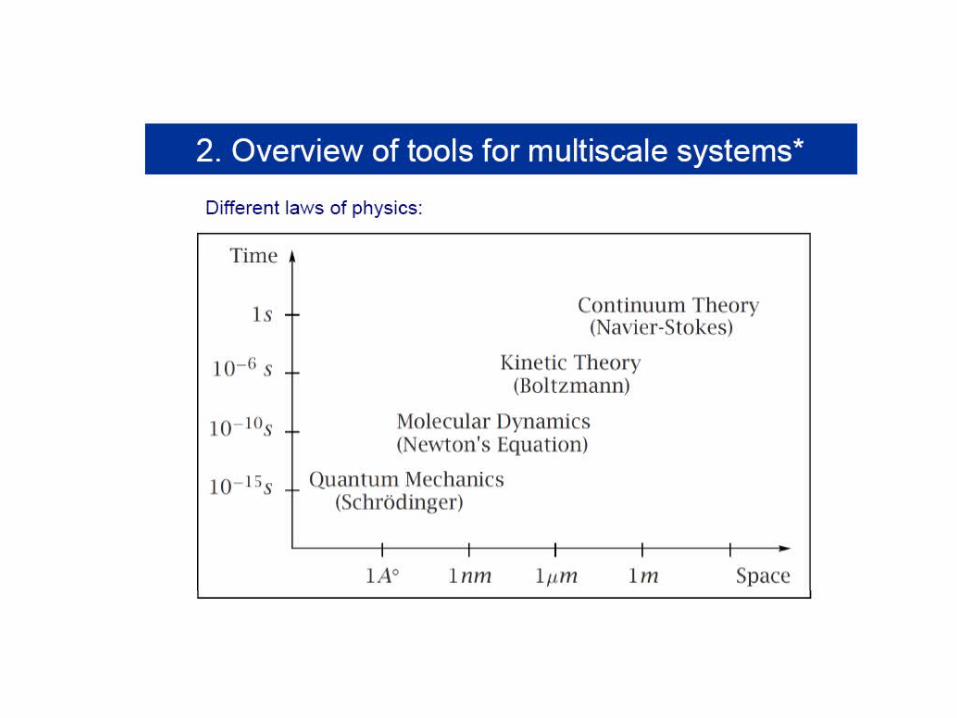
(fs) 10-15
(ps) 10-12
(ns) 10-9
(s) 10-6
(ms) 10-3
100
10-10 10-9 10-8 10-7 10-6 10-5 10-4
(nm) (m)LENGTH (m)
TIME (s)
Mesoscale methodsAtomistic SimulationMethods
Semi-empiricalmethods
Ab initiomethods
Monte CarloMolecular dynamics
tight-binding
Continuum
Finite elements methods
MethodsBased on SDSC Blue Horizon (SP3)512-1024 processors1.728 Tflops peak performanceCPU time = 1 week / processor
Multi-scale modeling
• Challenge: modeling a physical phenomenon from a broad range of perspectives, from the atomistic to the macroscopic end
• Ab initio methods: calculate materials properties from first principles, solving the quantum-mechanical Schrödinger (or Dirac) equation numerically
• Pros:– Give information on both the electronic and structural/mechanical
behavior– Can handle processes that involve bond breaking/formation, or
electronic rearrangement (e.g. chemical reactions).• Methods offer ways to systematically improve on the results,
making it easy to assess their quality.• Can (in principle) obtain essentially exact properties without any
input but the atoms conforming the system.
• Cons:
• Can handle only relatively small systems, about O(102) atoms.• Can only study fast processes, usually O(10) ps.• Numerically expensive!
Multi-scale modeling
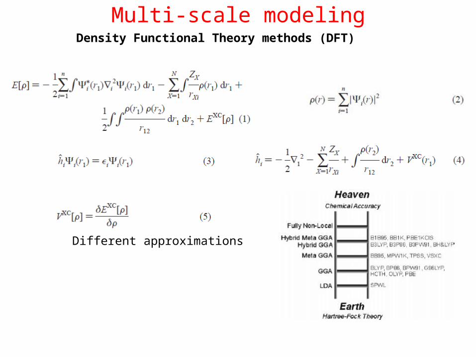
Different approximations
Multi-scale modelingDensity Functional Theory methods (DFT)
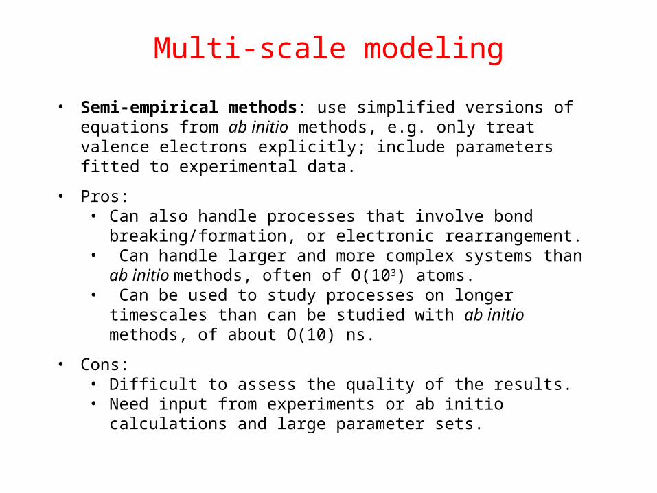
• Semi-empirical methods: use simplified versions of equations from ab initio methods, e.g. only treat valence electrons explicitly; include parameters fitted to experimental data.
• Pros:• Can also handle processes that involve bond breaking/formation, or
electronic rearrangement.• Can handle larger and more complex systems than ab initio
methods, often of O(103) atoms.• Can be used to study processes on longer timescales than can be
studied with ab initio methods, of about O(10) ns.
• Cons:• Difficult to assess the quality of the results.• Need input from experiments or ab initio calculations and large
parameter sets.
Multi-scale modeling

• Atomistic methods: use empirical or ab initio derived force fields, together with semi-classical statistical mechanics (SM), to determine thermodynamic (MC, MD) and transport (MD) properties of systems. SM solved ‘exactly’.
• Pros:• Can be used to determine the microscopic structure of more
complex systems, O(104-6) atoms.• Can study dynamical processes on longer timescales, up to O(1) s
• Cons:• Results depend on the quality of the force field used to represent
the system.• Many physical processes happen on length- and time-scales
inaccessible by these methods, e.g. diffusion in solids, many chemical reactions, protein folding, micellization.
Multi-scale modeling
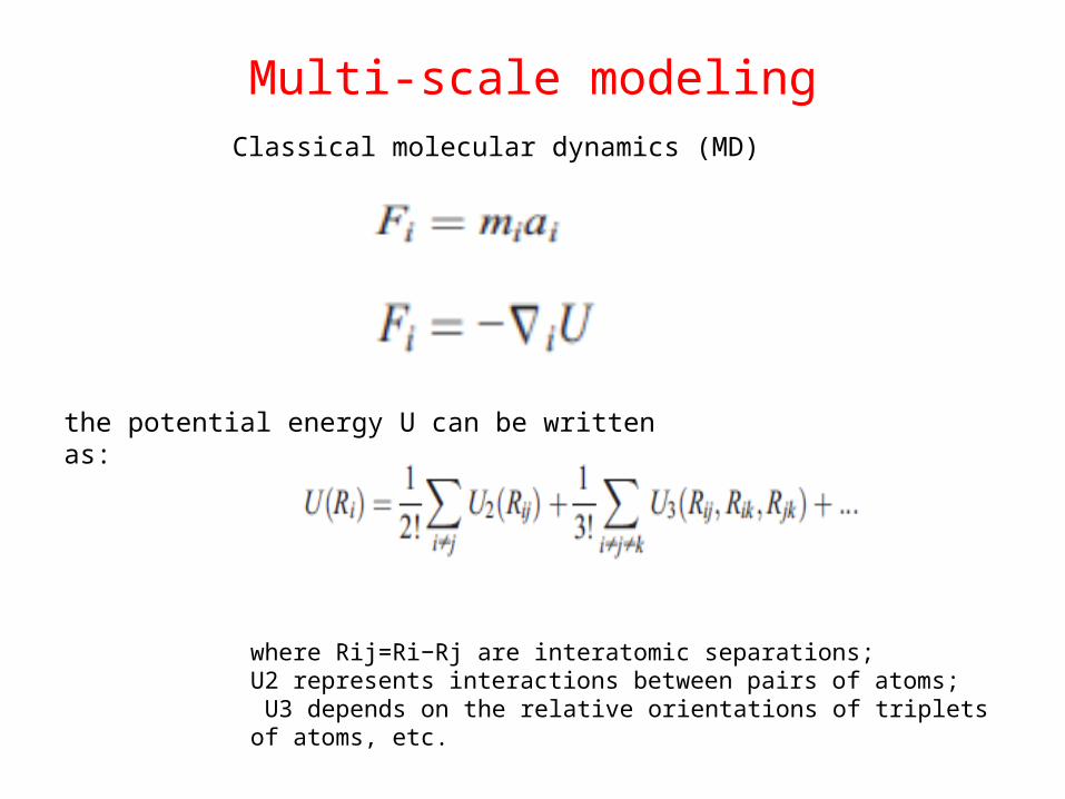
Multi-scale modelingClassical molecular dynamics (MD)
the potential energy U can be written as:
where Rij=Ri−Rj are interatomic separations;U2 represents interactions between pairs of atoms; U3 depends on the relative orientations of triplets of atoms, etc.
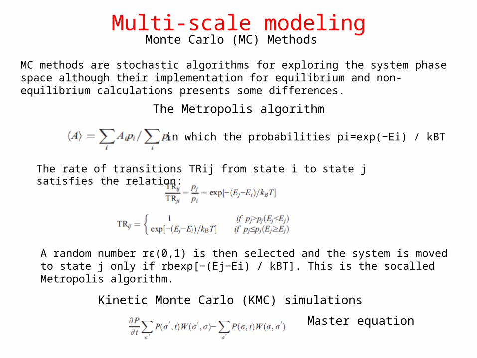
Kinetic Monte Carlo (KMC) simulations
Master equation
The Metropolis algorithm
Monte Carlo (MC) MethodsMulti-scale modeling
MC methods are stochastic algorithms for exploring the system phase space although their implementation for equilibrium and non-equilibrium calculations presents some differences.
in which the probabilities pi=exp(−Ei) / kBT
The rate of transitions TRij from state i to state j satisfies the relation:
A random number rε(0,1) is then selected and the system is moved to state j only if rbexp[−(Ej−Ei) / kBT]. This is the socalled Metropolis algorithm.
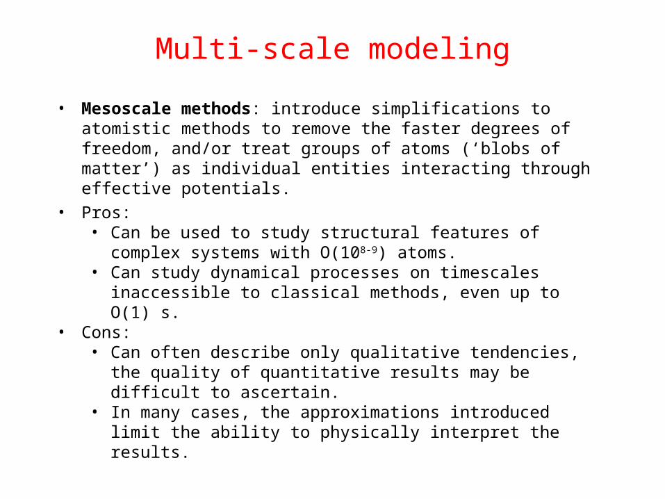
• Mesoscale methods: introduce simplifications to atomistic methods to remove the faster degrees of freedom, and/or treat groups of atoms (‘blobs of matter’) as individual entities interacting through effective potentials.
• Pros:• Can be used to study structural features of complex systems with
O(108-9) atoms.• Can study dynamical processes on timescales inaccessible to
classical methods, even up to O(1) s.• Cons:
• Can often describe only qualitative tendencies, the quality of quantitative results may be difficult to ascertain.
• In many cases, the approximations introduced limit the ability to physically interpret the results.
Multi-scale modeling

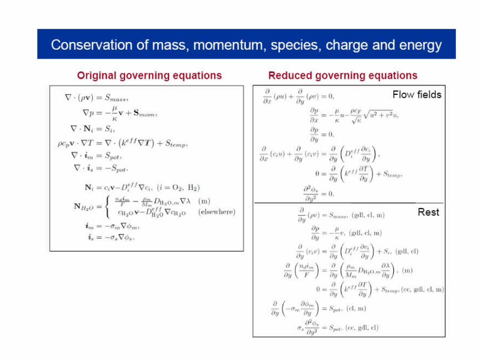
• Continuum methods: Assume that matter is continuous and treat the properties of the system as field quantities. Numerically solve balance equations coupled with phenomenological equations to predict the properties of the systems.
• Pros:
– Can in principle handle systems of any (macroscopic) size and dynamic processes on longer timescales.
• Cons:• Require input (elastic tensors, diffusion coefficients, equations of
state, etc.) from experiment or from a lower-scale methods that can be difficult to obtain.
• Cannot explain results that depend on the electronic or molecular level of detail.
Multi-scale modeling

• Connection between the scales:
“Upscaling”
Using results from a lower-scale calculation to obtain parameters for a higher-scale method. This is relatively easy to do; deductive approach. Examples:
• Calculation of phenomenological coefficients (e.g. elastic tensors, viscosities, diffusivities) from atomistic simulations for later use in a continuum model.
• Fitting of force-fields using ab initio results for later use in atomistic simulations.
• Deriving potential energy surface for a chemical reaction, to be used in atomistic MD simulations
• Deriving coarse-grained potentials for ‘blobs of matter’ from atomistic simulation, to be used in meso-scale simulations
Multi-scale modeling
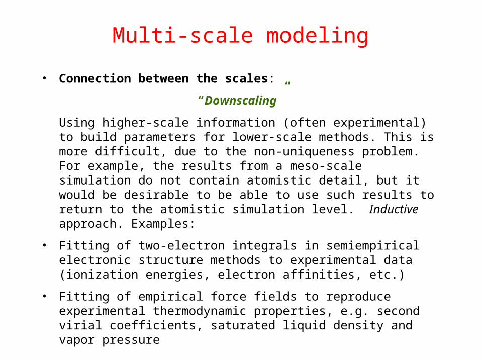
• Connection between the scales:
“Downscaling”
Using higher-scale information (often experimental) to build parameters for lower-scale methods. This is more difficult, due to the non-uniqueness problem. For example, the results from a meso-scale simulation do not contain atomistic detail, but it would be desirable to be able to use such results to return to the atomistic simulation level. Inductive approach. Examples:
• Fitting of two-electron integrals in semiempirical electronic structure methods to experimental data (ionization energies, electron affinities, etc.)
• Fitting of empirical force fields to reproduce experimental thermodynamic properties, e.g. second virial coefficients, saturated liquid density and vapor pressure
Multi-scale modeling
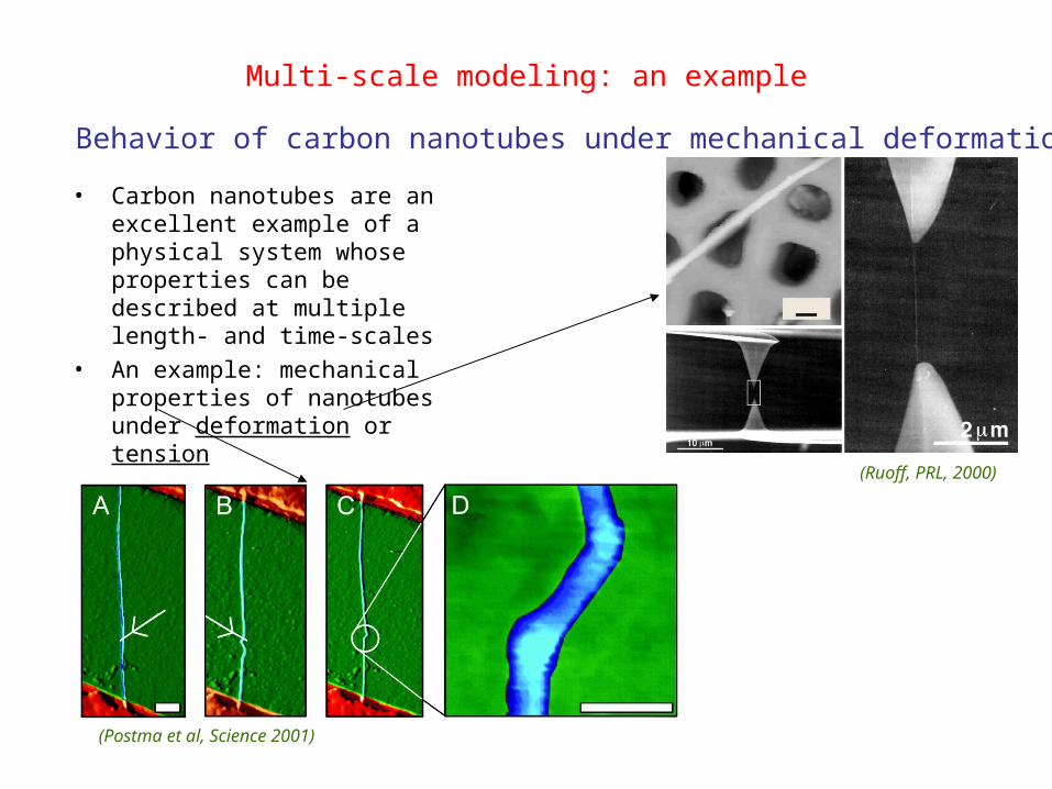
• Carbon nanotubes are an excellent example of a physical system whose properties can be described at multiple length- and time-scales
• An example: mechanical properties of nanotubes under deformation or tension
(Postma et al, Science 2001)
Multi-scale modeling: an example
Behavior of carbon nanotubes under mechanical deformations
(Ruoff, PRL, 2000)
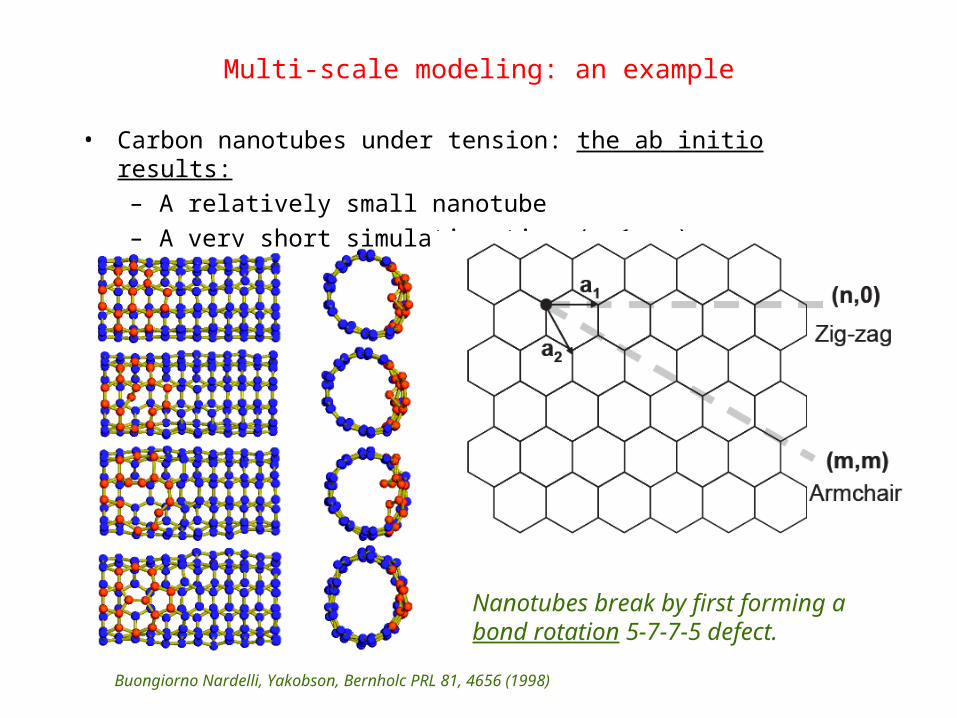
• Carbon nanotubes under tension: the ab initio results:
– A relatively small nanotube
– A very short simulation time (~ 1 ps)
Nanotubes break by first forming a bond rotation 5-7-7-5 defect.
Buongiorno Nardelli, Yakobson, Bernholc PRL 81, 4656 (1998)
Multi-scale modeling: an example

• Carbon nanotubes under tension: the atomistic results:– Expansion to a larger system and longer simulation times allows
exploration and discovery of new behaviors
For low strain values and high temperatures the (5775) defect behaves as a dislocation loop made up of two edge dislocations: (57) and (75). The two dislocations can migrate on the nanotube wall through a sequence of bond rotations PLASTIC BEHAVIOR
Buongiorno Nardelli, Yakobson, Bernholc PRL 81, 4656 (1998)
Multi-scale modeling: an example
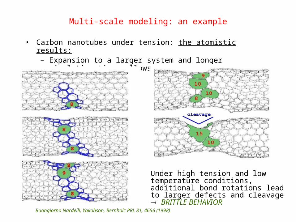
• Carbon nanotubes under tension: the atomistic results:– Expansion to a larger system and longer simulation times allows
exploration and discovery of new behaviors
Under high tension and low temperature conditions, additional bond rotations lead to larger defects and cleavage BRITTLE BEHAVIOR
Buongiorno Nardelli, Yakobson, Bernholc PRL 81, 4656 (1998)
Multi-scale modeling: an example
Multi-scale modeling: an example
A. DKHISSI , [email protected]

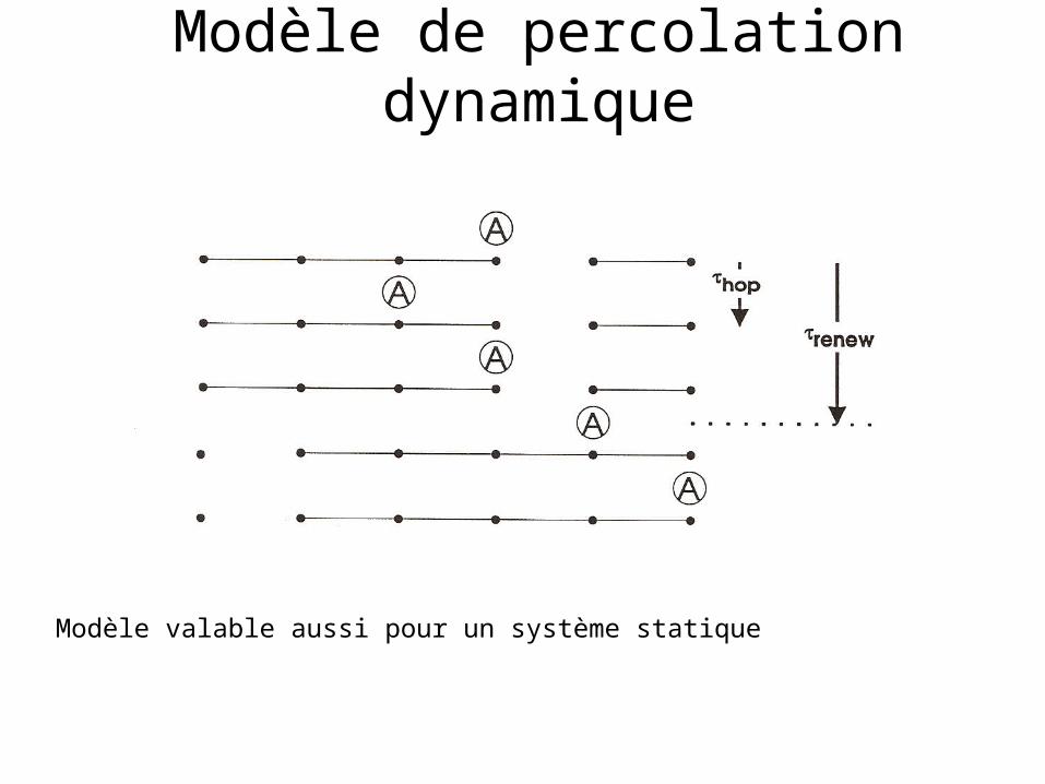
Modèle de percolation dynamique
Modèle valable aussi pour un système statique
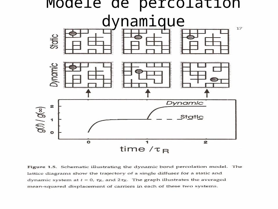
Modèle de percolation dynamique
A. DKHISSI , [email protected]
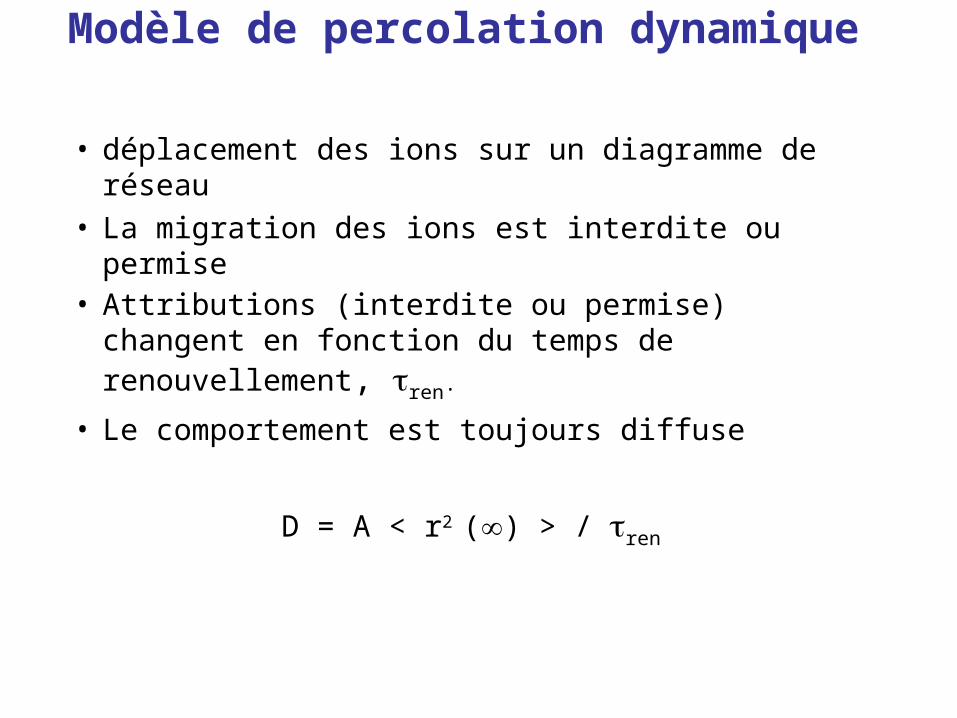
Modèle de percolation dynamique
• déplacement des ions sur un diagramme de réseau
• La migration des ions est interdite ou permise• Attributions (interdite ou permise) changent
en fonction du temps de renouvellement, ren.
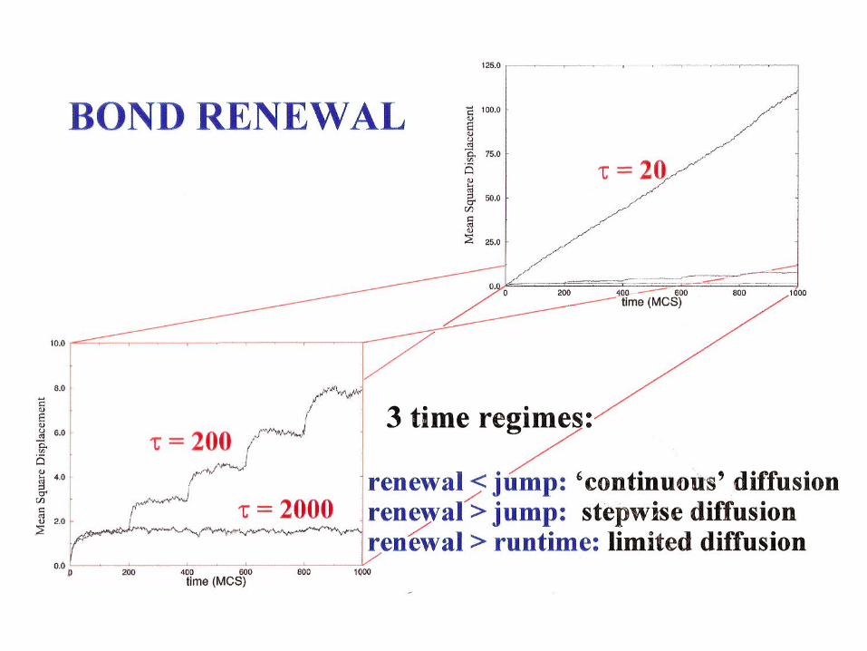
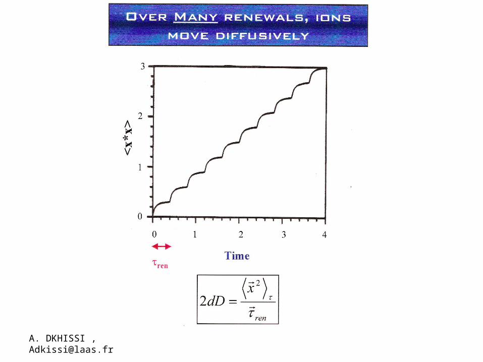
• Le comportement est toujours diffuse
D = A < r2 () > / ren