122
Introduction to partial differential equations 802635S Lecture Notes 3 rd Edition Valeriy Serov University of Oulu 2011 Edited by Markus Harju

Introduction to partial differential equations
802635S
Lecture Notes3rd Edition
Valeriy SerovUniversity of Oulu
2011
Edited by Markus Harju

Contents
0 Preliminaries 1
1 Local Existence Theory 10
2 Fourier Series 23
3 One-dimensional Heat Equation 32
4 One-dimensional Wave Equation 44
5 Laplace Equation in Rectangle and in Disk 51
6 The Laplace Operator 57
7 The Dirichlet and Neumann Problems 70
8 Layer Potentials 82
9 The Heat Operator 100
10 The Wave Operator 108
Index 119
i

0 Preliminaries
We consider Euclidean space Rn, n ≥ 1 with elements x = (x1, . . . , xn). The Euclideanlength of x is defined by
|x| =√x21 + · · ·+ x2n
and the standard inner product by
(x, y) = x1y1 + · · ·+ xnyn.
We use the Cauchy-Schwarz-Bunjakovskii inequality in Rn
|(x, y)| ≤ |x| · |y|.
By BR(x) we denote the ball of radius R > 0 with center x
BR(x) := y ∈ Rn : |x− y| < R.
We say that Ω ⊂ Rn, n ≥ 2 is an open set if for any x ∈ Ω there is R > 0 such that
BR(x) ⊂ Ω.
If n = 1 by open set we mean the open interval (a, b), a < b.An n-tuple α = (α1, . . . , αn) of non-negative integers will be called a multi-index .
We define
(i) |α| =∑nj=1 αj
(ii) α + β = (α1 + β1, . . . , αn + βn) with |α + β| = |α|+ |β|
(iii) α! = α1! · · ·αn! with 0! = 1
(iv) α ≥ β if and only if αj ≥ βj for each j = 1, 2, . . . , n. Moreover, α > β if andonly if α ≥ β and there exists j0 such that αj0 > βj0 .
(v) if α ≥ β then α− β = (α1 − β1, . . . , αn − βn) and |α− β| = |α| − |β|.
(vi) for x ∈ Rn we definexα = xα1
1 · · · xαnn
with 00 = 1.
We will use the shorthand notation
∂j =∂
∂xj, ∂α = ∂α1
1 · · · ∂αnn ≡ ∂|α|
∂xα11 · · · ∂xαn
n
.
This text assumes that the reader is familiar also with the following concepts:
1) Lebesgue integral in a bounded domain Ω ⊂ Rn and in Rn.
1

2) Banach spaces (Lp, 1 ≤ p ≤ ∞, Ck) and Hilbert spaces (L2): If 1 ≤ p <∞ thenwe set
Lp(Ω) := f : Ω → Cmeasurable : ‖f‖Lp(Ω) :=
(∫
Ω
|f(x)|pdx)1/p
<∞
while
L∞(Ω) := f : Ω → Cmeasurable : ‖f‖L∞(Ω) := ess supx∈Ω
|f(x)| <∞.
Moreover
Ck(Ω) := f : Ω → C : ‖f‖Ck(Ω) := maxx∈Ω
∑
|α|≤k|∂αf(x)| <∞,
where Ω is the closure of Ω. We say that f ∈ C∞(Ω) if f ∈ Ck(Ω1) for all k ∈ N
and for all bounded subsets Ω1 ⊂ Ω. The space C∞(Ω) is not a normed space.The inner product in L2(Ω) is denoted by
(f, g)L2(Ω) =
∫
Ω
f(x)g(x)dx.
Also in L2(Ω), the duality pairing is given by
〈f, g〉L2(Ω) =
∫
Ω
f(x)g(x)dx.
3) Holder’s inequality: Let 1 ≤ p ≤ ∞, u ∈ Lp and v ∈ Lp′with
1
p+
1
p′= 1.
Then uv ∈ L1 and∫
Ω
|u(x)v(x)|dx ≤(∫
Ω
|u(x)|pdx) 1
p(∫
Ω
|v(x)|p′dx) 1
p′
,
where the Holder conjugate exponent p′ of p is obtained via
p′ =p
p− 1
with the understanding that p′ = ∞ if p = 1 and p′ = 1 if p = ∞.
4) Lebesgue’s theorem about dominated convergence:
Let A ⊂ Rn be measurable and let fk∞k=1 be a sequence of measurable functionsconverging to f(x) point-wise in A. If there exists function g ∈ L1(A) such that|fk(x)| ≤ g(x) in A, then f ∈ L1(A) and
limk→∞
∫
A
fk(x)dx =
∫
A
f(x)dx.
2

5) Fubini’s theorem about the interchange of the order of integration:∫
X×Y|f(x, y)|dxdy =
∫
X
dx
(∫
Y
|f(x, y)|dy)
=
∫
Y
dy
(∫
X
|f(x, y)|dx),
if one of the three integrals exists.
Exercise 1. Prove the generalized Leibnitz formula
∂α(fg) =∑
β≤αCβα∂
βf∂α−βg,
where the generalized binomial coefficients are defined as
Cβα =
α!
β!(α− β)!= Cα−β
α .
Hypersurface
A set S ⊂ Rn is called hypersurface of class Ck, k = 1, 2, . . . ,∞, if for any x0 ∈ S thereis an open set V ⊂ Rn containing x0 and a real-valued function ϕ ∈ Ck(V ) such that
∇ϕ ≡ (∂1ϕ, . . . ∂nϕ) 6= 0 on S ∩ V
S ∩ V = x ∈ V : ϕ(x) = 0 .By implicit function theorem we can solve the equation ϕ(x) = 0 near x0 to obtain
xn = ψ(x1, . . . , xn−1)
for some Ck function ψ. A neighborhood of x0 in S can then be mapped to a piece ofthe hyperplane xn = 0 by
x 7→ (x′, xn − ψ(x′)),
where x′ = (x1, . . . , xn−1). The vector ∇ϕ is perpendicular to S at x ∈ S ∩ V . Thevector ν(x) which is defined as
ν(x) := ± ∇ϕ|∇ϕ|
is called the normal to S at x. It can be proved that
ν(x) = ± (∇ψ,−1)√|∇ψ|2 + 1
.
If S is the boundary of a domain Ω ⊂ Rn, n ≥ 2 we always choose the orientation sothat ν(x) points out of Ω and define the normal derivative of u on S by
∂νu := ν · ∇u ≡ ν1∂u
∂x1+ · · ·+ νn
∂u
∂xn.
Thus ν and ∂νu are Ck−1 functions.
Example 0.1. Let Sr(y) = x ∈ Rn : |x− y| = r. Then
ν(x) =x− y
rand ∂ν =
1
r
n∑
j=1
(xj − yj)∂
∂xj.
3

The divergence theorem
Let Ω ⊂ Rn be a bounded domain with C1 boundary S = ∂Ω and let F be a C1 vectorfield on Ω. Then ∫
Ω
∇ · Fdx =
∫
S
F · νdσ(x).
Corollary (Integration by parts). Let f and g be C1 functions on Ω. Then∫
Ω
∂jf · gdx = −∫
Ω
f · ∂jgdx+∫
S
f · gνjdσ(x).
Let f and g be locally integrable functions on Rn, i.e. integrable on any boundedset from Rn. The convolution f ∗ g of f and g is defined by
(f ∗ g)(x) =∫
Rn
f(x− y)g(y)dy = (g ∗ f)(x),
provided that the integral in question exists. The basic theorem on the existence ofconvolutions is the following (Young’s inequality for convolution):
Proposition 1 (Young’s inequality). Let f ∈ L1(Rn) and g ∈ Lp(Rn), 1 ≤ p ≤ ∞.Then f ∗ g ∈ Lp(Rn) and
‖f ∗ g‖Lp ≤ ‖f‖L1 ‖g‖Lp .
Proof. Let p = ∞. Then
|(f ∗ g)(x)| ≤∫
Rn
|f(x− y)||g(y)|dy ≤ ‖g‖L∞
∫
Rn
|f(x− y)|dy = ‖g‖L∞ ‖f‖L1 .
Let 1 ≤ p < ∞ now. Then it follows from Holder’s inequality and Fubini’s theoremthat
∫
Rn
|(f ∗ g)(x)|pdx ≤∫
Rn
(∫
Rn
|f(x− y)||g(y)|dy)p
dx
≤∫
Rn
(∫
Rn
|f(x− y)|dy)p/p′ ∫
Rn
|f(x− y)||g(y)|pdydx
≤ ‖f‖p/p′L1
∫
Rn
∫
Rn
|f(x− y)||g(y)|pdydx
≤ ‖f‖p/p′L1
∫
Rn
|g(y)|pdy∫
Rn
|f(x− y)|dx
= ‖f‖p/p′L1 ‖g‖pLp ‖f‖L1 = ‖f‖p/p′+1
L1 ‖g‖pLp .
Thus, we have finally
‖f ∗ g‖Lp ≤ ‖f‖1/p′+1/p
L1 ‖g‖Lp = ‖f‖L1 ‖g‖Lp .
4

Exercise 2. Suppose 1 ≤ p, q, r ≤ ∞ and 1p+ 1
q= 1
r+ 1. Prove that if f ∈ Lp(Rn)
and g ∈ Lq(Rn) then f ∗ g ∈ Lr(Rn) and
‖f ∗ g‖r ≤ ‖f‖p ‖g‖q .
In particular,‖f ∗ g‖L∞ ≤ ‖f‖Lp ‖g‖Lp′ .
Definition. Let u ∈ L1(Rn) with∫
Rn
u(x)dx = 1.
Then uε(x) := ε−nu(x/ε), ε > 0 is called an approximation to the identity .
Proposition 2. Let uε(x) be an approximation to the identity. Then for any functionϕ ∈ L∞(Rn) which is continuous at 0 we have
limε→0+
∫
Rn
uε(x)ϕ(x)dx = ϕ(0).
Proof. Since uε(x) is an approximation to the identity we have∫
Rn
uε(x)ϕ(x)dx− ϕ(0) =
∫
Rn
uε(x)(ϕ(x)− ϕ(0))dx
and thus∣∣∣∣∫
Rn
uε(x)ϕ(x)dx− ϕ(0)
∣∣∣∣ ≤∫
|x|≤√ε
|uε(x)||ϕ(x)− ϕ(0)|dx
+
∫
|x|>√ε
|uε(x)||ϕ(x)− ϕ(0)|dx
≤ sup|x|≤√
ε
|ϕ(x)− ϕ(0)|∫
Rn
|uε(x)|dx+ 2 ‖ϕ‖L∞
∫
|x|>√ε
|uε(x)|dx
≤ sup|x|≤√
ε
|ϕ(x)− ϕ(0)| · ‖u‖L1 + 2 ‖ϕ‖L∞
∫
|y|>1/√ε
|u(y)|dy → 0
as ε→ 0.
Example 0.2. Let u(x) be defined as
u(x) =
sinx1
2· · · sinxn
2, x ∈ [0, π]n
0, x /∈ [0, π]n.
Then uε(x) is an approximation to the identity and
limε→0
(2ε)−n∫ επ
0
· · ·∫ επ
0
n∏
j=1
sinxjεϕ(x)dx = ϕ(0).
5

Fourier transform
If f ∈ L1(Rn) its Fourier transform f or F(f) is the bounded function on Rn definedby
f(ξ) = (2π)−n/2∫
Rn
e−ix·ξf(x)dx.
Clearly f(ξ) is well-defined for all ξ and∥∥∥f∥∥∥∞
≤ (2π)−n/2 ‖f‖1 .
The Riemann-Lebesgue lemma
If f ∈ L1(Rn) then f is continuous and tends to zero at infinity.
Proof. Let us first prove that Ff(ξ) is continuous (even uniformly continuous) in Rn.Indeed,
|Ff(ξ + h)−Ff(ξ)| ≤ (2π)−n/2∫
Rn
|f(x)| · |e−i(x,h) − 1|dx
≤∫
|x||h|≤√
|h||f(x)||x||h|dx+ 2
∫
|x||h|>√
|h||f(x)|dx
≤√|h| ‖f‖L1 + 2
∫
|x|>1/√
|h||f(x)|dx→ 0
as |h| → 0 since f ∈ L1(Rn).To prove that Ff(ξ) → 0 as |ξ| → 0 we proceed as follows. Since eiπ = −1 then
2Ff(ξ) = (2π)−n/2∫
Rn
f(x)e−i(x,ξ)dx− (2π)−n/2∫
Rn
f(x)e−i(x−πξ/|ξ|2,ξ)dx
= (2π)−n/2∫
Rn
f(x)e−i(x,ξ)dx− (2π)−n/2∫
Rn
f(y + πξ/|ξ|2)e−i(y,ξ)dy
= −(2π)−n/2∫
Rn
(f(x+ πξ/|ξ|2)− f(x))e−i(x,ξ)dx.
Hence
2|Ff(ξ)| ≤ (2π)−n/2∫
Rn
|f(x+ πξ/|ξ|2)− f(x)|dx
= (2π)−n/2∥∥f(·+ πξ/|ξ|2)− f(·)
∥∥L1 → 0
as |ξ| → ∞ since f ∈ L1(Rn).
Exercise 3. Prove that if f, g ∈ L1(Rn) then f ∗ g = (2π)n/2f g.
Exercise 4. Suppose f ∈ L1(Rn). Prove that
1. If fh(x) = f(x+ h) then fh = eih·ξf .
6

2. If T : Rn → Rn is linear and invertible then f T = |detT |−1f ((T−1)′ξ), whereT ′ is the adjoint matrix.
3. If T is rotation, that is T ′ = T−1 (and |detT | = 1) then f T = f T .
Exercise 5. Prove that
∂αf = (−ix)αf, ∂αf = (iξ)αf .
Exercise 6. Prove that if f, g ∈ L1(Rn) then∫
Rn
f(ξ)g(ξ)dξ =
∫
Rn
f(ξ)g(ξ)dξ.
For f ∈ L1(Rn) define the inverse Fourier transform of f by
F−1f(x) = (2π)−n/2∫
Rn
eix·ξf(ξ)dξ.
It is clear thatF−1f(x) = Ff(−x), F−1f = F(f)
and for f, g ∈ L1(Rn)(Ff, g)L2 = (f,F−1g)L2 .
The Schwartz space S(Rn) is defined as
S(Rn) =
f ∈ C∞(Rn) : sup
x∈Rn
|xα∂βf(x)| <∞, for any multi-indicesα and β
.
The Fourier inversion formula
If f ∈ S(Rn) then (F−1F)f = f .
Exercise 7. Prove the Fourier inversion formula for f ∈ S(Rn).
The Plancherel theorem
The Fourier transform on S extends uniquely to a unitary isomorphism of L2(Rn) ontoitself, i.e. ∥∥∥f
∥∥∥2= ‖f‖2 .
This formula is called the Parseval equality.The support of a function f : Rn → C, denoted by supp f , is the set
supp f = x ∈ Rn : f(x) 6= 0.
Exercise 8. Prove that if f ∈ L1(Rn) has compact support then f extends to an entireholomorphic function on Cn.
7

Exercise 9. Prove that if f ∈ C∞0 (Rn) i.e. f ∈ C∞(Rn) with compact support, is
supported in x ∈ Rn : |x| ≤ R then for any multi-index α we have
|(iξ)αf(ξ)| ≤ (2π)−n/2eR|Im ξ| ‖∂αf‖1 ,
that is, f(ξ) is rapidly decaying as |Re ξ| → ∞ when |Im ξ| remains bounded.
Distributions
We say that ϕj → ϕ in C∞0 (Ω),Ω ⊂ Rn open, if ϕj are all supported in a common
compact set K ⊂ Ω and
supx∈K
|∂αϕj(x)− ∂αϕ(x)| → 0, j → ∞
for all α. A distribution on Ω is a linear functional u on C∞0 (Ω) that is continuous, i.e.,
1. u : C∞0 (Ω) → C. The action of u to ϕ ∈ C∞
0 (Ω) is denoted by 〈u, ϕ〉. The set ofall distributions is denoted by D′(Ω).
2. 〈u, c1ϕ1 + c2ϕ2〉 = c1〈u, ϕ1〉+ c2〈u, ϕ2〉
3. If ϕj → ϕ in C∞0 (Ω) then 〈u, ϕj〉 → 〈u, ϕ〉 in C as j → ∞. It is equivalent to the
following condition: for any K ⊂ Ω there is a constant CK and an integer NK
such that for all ϕ ∈ C∞0 (K),
|〈u, ϕ〉| ≤ CK∑
|α|≤NK
‖∂αϕ‖∞ .
Remark. If u ∈ L1loc(Ω),Ω ⊂ Rn open, then u can be regarded as a distribution (in
that case a regular distribution) as follows:
〈u, ϕ〉 :=∫
Ω
u(x)ϕ(x)dx, ϕ ∈ C∞0 (Ω).
The Dirac δ-function
The δ-function is defined as
〈δ, ϕ〉 = ϕ(0), ϕ ∈ C∞0 (Ω).
It is not a regular distribution.
Example 0.3. Let uε(x) be an approximation to the identity. Then
uε(ξ) = (2π)−n/2∫
Rn
ε−nu(x/ε)e−i(x,ξ)dx = (2π)−n/2∫
Rn
u(y)e−i(y,eξ)dy = u(εξ).
In particular,limε→0+
uε(ξ) = limε→0+
u(εξ) = (2π)−n/2.
Applying Proposition 2 we may conclude that
8
1) limε→0+〈uε, ϕ〉 = ϕ(0) i.e. limε→0+ uε = δ in the sense of distributions, and
2) δ = (2π)−n/2 · 1.
We can extend the operations from functions to distributions as follows:
〈∂αu, ϕ〉 = 〈u, (−1)|α|∂αϕ〉,
〈fu, ϕ〉 = 〈u, fϕ〉, f ∈ C∞(Ω),
〈u ∗ ψ, ϕ〉 = 〈u, ϕ ∗ ψ〉, ψ ∈ C∞0 (Ω),
where ψ(x) = ψ(−x). It is possible to show that u ∗ ψ is actually a C∞ function and
∂α(u ∗ ψ) = u ∗ ∂αψ.
A tempered distribution is a continuous linear functional on S(Rn). In addition to thepreceding operations for the tempered distributions we can define the Fourier transformby
〈u, ϕ〉 = 〈u, ϕ〉, ϕ ∈ S.
Exercise 10. Prove that if u is a tempered distribution and ψ ∈ S then
u ∗ ψ = (2π)n/2ψu.
Exercise 11. Prove that
1. δ = (2π)−n/2 · 1, 1 = (2π)n/2δ
2. ∂αδ = (iξ)α(2π)−n/2
3. xα = i|α|∂α(1) = i|α|(2π)n/2∂αδ.
9
1 Local Existence Theory
A partial differential equation of order k ∈ N is an equation of the form
F(x, (∂αu)|α|≤k
)= 0, (1.1)
where F is a function of the variables x ∈ Ω ⊂ Rn, n ≥ 2,Ω an open set, and (uα)|α|≤k.A complex-valued function u(x) on Ω is a classical solution of (1.1) if the derivatives
∂αu occurring in F exist on Ω and
F(x, (∂αu(x))|α|≤k
)= 0
pointwise for all x ∈ Ω. The equation (1.1) is called linear if it can be written as
∑
|α|≤kaα(x)∂
αu(x) = f(x) (1.2)
for some known functions aα and f . In this case we speak about the (linear) differentialoperator
L(x, ∂) ≡∑
|α|≤kaα(x)∂
α
and write (1.2) simply as Lu = f. If the coefficients aα(x) belong to C∞(Ω) we can apply
the operator L to any distribution u ∈ D′(Ω) and u is called a distributional solution(or weak solution) of (1.2) if the equation (1.2) holds in the sense of distributions, i.e.
∑
|α|≤k(−1)|α|〈u, ∂α(aαϕ)〉 = 〈f, ϕ〉,
where ϕ ∈ C∞0 (Ω). Let us list some examples. Here and throughout we denote
ut =∂u∂t, utt =
∂2u∂t2
and so forth.
1. The eikonal equation|∇u|2 = c2,
where ∇u = (∂1u, . . . , ∂nu) is the gradient of u.
2. a) Heat (or evolution) equation
ut = k∆u
b) Wave equationutt = c2∆u
c) Poisson equation∆u = f,
where ∆ ≡ ∇·∇ = ∂21 + · · ·+∂2n is the Laplacian (or the Laplace operator).
10
3. The telegrapher’s equation
utt = c2∆u− αut −m2u
4. Sine-Gordon equationutt = c2∆u− sin u
5. The biharmonic equation∆2u ≡ ∆(∆u) = 0
6. The Korteweg-de Vries equation
ut + cu · ux + uxxx = 0.
In the linear case, a simple measure of the ”strength” of a differential operator isprovided by the notion of characteristics. If L(x, ∂) =
∑|α|≤k aα(x)∂
α then its charac-
teristic form (or principal symbol) at x ∈ Ω is the homogeneous polynomial of degreek defined by
χL(x, ξ) =∑
|α|=kaα(x)ξ
α, ξ ∈ Rn.
A nonzero ξ is called characteristic for L at x if χL(x, ξ) = 0 and the set of all such ξis called the characteristic variety of L at x, denoted by charx(L). In other words,
charx(L) = ξ 6= 0 : χL(x, ξ) = 0 .
In particular, L is said to be elliptic at x if charx(L) = ∅ and elliptic in Ω if it is ellipticat every x ∈ Ω.
Example 1.1. 1. L = ∂1∂2, charx(L) = ξ ∈ R2 : ξ1 = 0or ξ2 = 0, ξ21 + ξ22 > 0 .
2. L = 12(∂1 + i∂2) is the Cauchy-Riemann operator on R2. It is elliptic in R2.
3. L = ∆ is elliptic in Rn.
4. L = ∂1 −∑n
j=2 ∂2j , charx(L) = ξ ∈ Rn\ 0 : ξj = 0, j = 2, 3, . . . , n .
5. L = ∂21 −∑n
j=2 ∂2j , charx(L) =
ξ ∈ Rn\ 0 : ξ21 =
∑nj=2 ξ
2j
.
Let ν(x) be the normal to S at x. A hypersurface S is called characteristic for Lat x ∈ S if ν(x) ∈ charx(L), i.e.
χL(x, ν(x)) = 0
and S is called non-characteristic if it is not characteristic at any point, that is, forany x ∈ S
χL(x, ν(x)) 6= 0.
11

Let us consider the linear equation of the first order
Lu ≡n∑
j=1
aj(x)∂ju+ b(x)u = f(x), (1.3)
where aj, b and f are assumed to be C1 functions of x. We assume also that aj, b and fare real-valued. Suppose we wish to find a solution u of (1.3) with given initial valuesu = g on the hypersurface S (g is also real-valued). It is clear that
charx(L) =ξ 6= 0 : ~A · ξ = 0
,
where ~A = (a1, . . . , an). It implies that charx(L)∪0 is the hyperplane orthogonal to~A and therefore, S is characteristic at x if and only if ~A is tangent to S at x ( ~A ·ν = 0).Then
n∑
j=1
aj(x)∂ju(x) =n∑
j=1
aj(x)∂jg(x), x ∈ S,
is completely determined as certain directional derivatives of ϕ (see the definition ofS) along S at x, and it may be impossible to make it equal to f(x) − b(x)u(x) (inorder to satisfy (1.3)). Indeed, let us assume that u1 and u2 have the same value g onS. This means that u1 − u2 = 0 on S or (more or less equivalently)
u1 − u2 = ϕ · γ,
where ϕ = 0 on S (ϕ defines this surface) and γ 6= 0 on S. Next,
( ~A · ∇)u1 − ( ~A · ∇)u2 = ( ~A · ∇)(ϕγ) = γ( ~A · ∇)ϕ+ ϕ( ~A · ∇)γ = 0,
since S is characteristic for L (( ~A · ∇)ϕ = 0 ⇔ ( ~A · ∇|∇|)ϕ = 0 ⇔ ~A · ν = 0). That’s
why to make the initial value problem well-defined we must assume that S is non-characteristic for this problem.
Let us assume that S is non-characteristic for L and u = g on S. We define theintegral curves for (1.3) as the parametrized curves x(t) that satisfy the system
x = ~A(x), x = x(t) = (x1(t), . . . , xn(t)) (1.4)
of ordinary differential equations, where
x = (x′1(t), . . . , x′n(t)).
Along one of those curves a solution u of (1.3) must satisfy
du
dt=
d
dt(u(x(t))) =
n∑
j=1
xj∂u
∂xj= ( ~A · ∇)u = f − bu ≡ f(x(t))− bu(x(t))
12
ordu
dt= f − bu. (1.5)
By the existence and uniqueness theorem for ordinary differential equations there is aunique solution (unique curve) of (1.4) with x(0) = x0. Along this curve the solutionu(x) of (1.3) must be the solution of (1.5) with u(0) = u(x(0)) = u(x0) = g(x0).Moreover, since S is non-characteristic, x(t) /∈ S for t 6= 0, at least for small t, and thecurves x(t) fill out a neighborhood of S. Thus we have proved the following theorem.
Theorem 1. Assume that S is a surface of class C1 which is non-characteristic for(1.3), and that aj, b, f and g are C1 and real-valued functions. Then for any sufficientlysmall neighborhood U of S in Rn there is a unique solution u ∈ C1 of (1.3) on U thatsatisfies u = g on S.
Remark. The method which was presented above is called themethod of characteristics .
Let us consider some examples where we apply the method of characteristics.
Example 1.2. In R3, solve x1∂1u+2x2∂2u+∂3u = 3u with u = g(x1, x2) on the planex3 = 0.
Since S = x ∈ R3 : x3 = 0 then ν(x) = (0, 0, 1) and since χL(x, ξ) = x1ξ1 +2x2ξ2 + ξ3 we have
χL(x, ν(x)) = x1 · 0 + 2x2 · 0 + 1 · 1 = 1 6= 0
so that S is non-characteristic. The system (1.4)-(1.5) to be solved is
x1 = x1, x2 = 2x2, x3 = 1, u = 3u
with initial conditions
(x1, x2, x3)|t=0 = (x01, x02, 0), u(0) = g(x01, x
02)
on S. We obtain
x1 = x01et, x2 = x02e
2t, x3 = t, u = g(x01, x02)e
3t.
These equations imply
x01 = x1e−t = x1e
−x3 , x02 = x2e−2t = x2e
−2x3 .
Thereforeu(x) = u(x1, x2, x3) = g(x1e
−x3 , x2e−2x3)e3x3 .
Example 1.3. In R3, solve ∂1u+ x1∂2u− ∂3u = u with u(x1, x2, 1) = x1 + x2.Since S = x ∈ R3 : x3 = 1 then ν(x) = (0, 0, 1). That’s why
χL(x, ν(x)) = 1 · 0 + x1 · 0− 1 · 1 = −1 6= 0
13

and S is non-characteristic. The system (1.4)-(1.5) for this problem becomes
x1 = 1, x2 = x1, x3 = −1, u = u
with(x1, x2, x3)|t=0 = (x01, x
02, 1), u(0) = x01 + x02.
We obtain
x1 = t+ x01, x2 =t2
2+ tx01 + x02, x3 = −t+ 1, u = (x01 + x02)e
t.
Then,t = 1− x3, x01 = x1 − t = x1 + x3 − 1,
x02 = x2 −(1− x3)
2
2− (1− x3)(x1 + x3 − 1) =
1
2− x1 + x2 − x3 + x1x3 +
x232
and, finally,
u =
(x232
+ x1x3 + x2 −1
2
)e1−x3 .
Now let us generalize this technique to quasi-linear equations or to the equationsof the form
n∑
j=1
aj(x, u)∂ju = b(x, u), (1.6)
where aj, b and u are real-valued. If u is a function of x, the normal to the graph of uin Rn+1 is proportional to (∇u,−1), so (1.6) just says that the vector field
~A(x, y) := (a1, . . . , an, b) ∈ Rn+1
is tangent to the graph y = u(x) at any point. This suggests that we look at the
integral curves of ~A in Rn+1 given by solving the ordinary differential equations
xj = aj(x, y), j = 1, 2, . . . , n, y = b(x, y).
Suppose u is a solution of (1.6). If we solve
xj = aj(x, u(x)), j = 1, 2, . . . , n,
with xj(0) = x0j then setting y(t) = u(x(t)) we obtain that
y =n∑
j=1
∂ju · xj =n∑
j=1
aj(x, u)∂ju = b(x, u) = b(x, y).
Suppose we are given initial data u = g on S. If we form the submanifold
S∗ := (x, g(x)) : x ∈ S
14

in Rn+1 then the graph of the solution should be the hypersurface generated by theintegral curves of ~A passing through S∗. Again, we need to assume that S is non-characteristic in a sense that the vector
(a1(x, g(x)), . . . , an(x, g(x))) , x ∈ S,
should not be tangent to S at x. If S is represented parametrically by a mapping~ϕ : Rn−1 → Rn (for example ~ϕ(x1, . . . , xn−1) = (x1, . . . , xn−1, ψ(x1, . . . , xn−1))) and wehave the coordinates x′ = (x1, . . . , xn−1) ∈ Rn−1 this condition is just
det
∂ϕ1
∂x1. . . ∂ϕ1
∂xn−1a1 (~ϕ(x
′), g(~ϕ(x′)))...
. . ....
...∂ϕn
∂x1. . . ∂ϕn
∂xn−1an (~ϕ(x
′), g(~ϕ(x′)))
6= 0.
Remark. If S is parametrized as
xn = ψ(x1, . . . , xn−1), x′ = (x1, . . . , xn−1) ∈ S ′ ⊂ Rn−1
then S can be represented also by
φ(x1, . . . , xn) = 0,
where φ(x1, . . . , xn) ≡ ψ(x′)− xn and ν(x) is proportional to
∇φ =
(∂ψ
∂x1, . . . ,
∂ψ
∂xn−1
,−1
).
Then S is non-characteristic if and only if
a1∂ψ
∂x1+ · · ·+ an−1
∂ψ
∂xn−1
− an 6= 0
or
det
1 0 · · · 0 a1 (x, g(x))0 1 · · · 0 a2 (x, g(x))...
.... . .
......
0 0 · · · 1 an−1 (x, g(x))∂ψ∂x1
· · · · · · ∂ψ∂xn−1
an (x, g(x))
6= 0,
where x ∈ S.
Example 1.4. In R2, solve u∂1u+ ∂2u = 1 with u = s/2 on the segment x1 = x2 = s,where s > 0, s 6= 2 is a parameter.
Since ~ϕ(s) = (s, s) then (x′ = x1 = s)
det
(∂x1∂s
a1(s, s, s/2)∂x2∂s
a2(s, s, s/2)
)= det
(1 s/21 1
)= 1− s/2 6= 0,
15
for s > 0, s 6= 2. The system (1.4)-(1.5) for this problem is
x1 = u, x2 = 1, u = 1
with
(x1, x2, u)|t=0 = (x01, x02,x012) = (s, s, s/2).
Thenu = t+ s/2, x2 = t+ s, x1 = t+ s/2
so that x1 =t2
2+ st
2+ s. This implies
x1 − x2 = t2/2 + t(s/2− 1).
For s and t in terms of x1 and x2 we obtain
s
2= 1 +
1
t
(x1 − x2 −
t2
2
), t =
2(x1 − x2)
x2 − 2.
Hence
u =2(x1 − x2)
x2 − 2+ 1 +
x1 − x2t
− t
2
=2(x1 − x2)
x2 − 2+ 1 +
x2 − 2
2− x1 − x2
x2 − 2
=x1 − x2x2 − 2
+ 1 +x2 − 2
2=x1 − x2x2 − 2
+x22
=2x1 − 4x2 + x22
2(x2 − 2).
Exercise 12. In R2, solve x21∂1u+ x22∂2u = u2 with u ≡ 1 when x2 = 2x1.
Exercise 13. In R2, solve u∂1u+ x2∂2u = x1 with u(x1, 1) = 2x1.
Example 1.5. Consider the Burgers equation
u∂1u+ ∂2u = 0
in R2 with u(x1, 0) = h(x1), where h is a known C1 function. It is clear that S :=x ∈ R2 : x2 = 0 is non-characteristic for this quasi-linear equation, since
det
(1 h(x1)0 1
)= 1 6= 0,
and ν(x) = (0, 1). Now we have to solve the ordinary differential equations
x1 = u, x2 = 1, u = 0
16

with(x1, x2, u)|t=0 =
(x01, 0, h(x
01)).
We obtainx2 = t, u ≡ h(x01), x1 = h(x01)t+ x01
so thatx1 − x2h(x
01)− x01 = 0.
Let us assume that−x2h′1(x01)− 1 6= 0.
By this condition last equation defines an implicit function x01 = g(x1, x2). That’s whythe solution u of the Burgers equation has the form
u(x1, x2) = h(g(x1, x2)).
Let us consider two particular cases:
1. If h(x01) = ax01 + b, a 6= 0, then
u(x1, x2) =ax1 + b
ax2 + 1, x2 6= −1
a.
2. If h(x01) = a(x01)2 + bx01 + c, a 6= 0, then
u(x1, x2) = a
(−x2b− 1 +
√(x2b+ 1)2 − 4ax2(cx2 − x1)
2ax2
)
+ b
(−x2b− 1 +
√(x2b+ 1)2 − 4ax2(cx2 − x1)
2ax2
)+ c,
with D = (x2b+ 1)2 − 4ax2(cx2 − x1) > 0.
Let us consider again the linear equation (1.2) of order k i.e.
∑
|α|≤kaα(x)∂
αu(x) = f(x).
Let S be a hypersurface of class Ck. If u is a Ck function defined near S, the quantities
u, ∂νu, . . . , ∂k−1ν u (1.7)
on S are called the Cauchy data of u on S. And the Cauchy problem is to solve (1.2)with the Cauchy data (1.7). We shall consider Rn, n ≥ 2, as Rn−1 ×R and denote thecoordinates by (x, t), where x = (x1, . . . , xn−1). We can make a change of coordinatesfrom Rn to Rn−1 × R so that x0 ∈ S is mapped to (0, 0) and a neighborhood of x0 in
17

S is mapped into the hyperplane t = 0. In that case ∂ν = ∂∂t
on S = (x, t) : t = 0and equation (1.2) can be written in the new coordinates as
∑
|α|+j≤kaα,j(x, t)∂
αx∂
jtu = f(x, t) (1.8)
with the Cauchy data
∂jtu(x, 0) = ϕj(x), j = 0, 1, . . . , k − 1. (1.9)
Since the normal ν = (0, 0, . . . , 0, 1) then the assumption ”S is non-characteristic”means that
χL(x, 0, ν(x, 0)) ≡ a0,k(x, 0) 6= 0.
Hence by continuity a0,k(x, t) 6= 0 for small t, and we can solve (1.8) for ∂kt u:
∂kt u(x, t) = (a0,k(x, t))−1
f −
∑
|α|+j≤k,j<kaα,j∂
αx∂
jtu
(1.10)
with the Cauchy data (1.9).
Example 1.6. The line t = 0 is characteristic for ∂x∂tu = 0 in R2. That’s whywe will have some problems with the solutions. Indeed, if u is a solution of thisequation with Cauchy data u(x, 0) = g0(x) and ∂tu(x, 0) = g1(x) then ∂xg1 = 0,that is, g1 ≡ constant. Thus the Cauchy problem is not solvable in general. Onthe other hand, if g1 is constant, then there is no uniqueness, because we can takeu(x, t) = g0(x) + f(t) with any f(t) such that f(0) = 0 and f ′(0) = g1.
Example 1.7. The line t = 0 is characteristic for ∂2xu− ∂tu = 0 in R2. Here if we aregiven u(x, 0) = g0(x) then ∂tu(x, 0) is already completely determined by ∂tu(x, 0) =g′′0(x). So, again the Cauchy problem has ”bad” behaviour.
Let us now formulate and give ”a sketch” of the proof of the famous Cauchy-Kowalevski theorem for linear case.
Theorem 2. If aα,j(x, t), ϕ0(x), . . . , ϕk−1(x) are analytic near the origin in Rn, thenthere is a neighborhood of the origin on which the Cauchy problem (1.10)-(1.9) has aunique analytic solution.
Proof. The uniqueness of analytic solution follows from the fact that an analytic func-tion is completely determined by the values of its derivatives at one point (see theTaylor formula or the Taylor series). Indeed, for all α and j = 0, 1, . . . , k − 1
∂αx∂jtu(x, 0) = ∂αxϕj(x).
That’s why
∂kt u|t=0 = (a0,k)−1
f(x, 0)−
∑
|α|+j≤k,j<kaα,j(x, 0)∂
αxϕj(x)
18

and moreover
∂kt u(x, t) = (a0,k)−1
f(x, t)−
∑
|α|+j≤k,j<kaα,j(x, t)∂
αx∂
jtu
.
Then all derivatives of u can be defined from this equation by
∂k+1t u = ∂t
(∂kt u).
Next, let us denote by yα,j = ∂αx∂jtu and by Y = (yα,j) this vector. Then equation
(1.10) can be rewritten as
y0,k = (a0,k)−1
f −
∑
|α|+j≤k,j<kaα,jyα,j
or
∂t (y0,k−1) = (a0,k)−1
f −
∑
|α|+j≤k,j<kaα,j∂xjy(α−~j),j
and therefore the Cauchy problem (1.10)-(1.9) becomes
∂tY =
∑n−1j=1 Aj∂xjY + B
Y (x, 0) = Φ(x), x ∈ Rn−1,(1.11)
where Y,B and Φ are analytic vector-valued functions and Aj’s are analytic matrix-valued functions. Without loss of generality we can assume that Φ ≡ 0. Let Y =(y1, . . . , yN ), B = (b1, . . . , bN), Aj = (a
(j)ml)
Nm,l=1. We seek a solution Y = (y1, . . . , yN ) in
the formym =
∑C
(m)α,j x
αtj, m = 1, 2, . . . , N.
The Cauchy data tell us that C(m)α,0 = 0 for all α and m, since we assumed Φ ≡ 0. To
determine C(m)α,j for j > 0, we substitute ym into (1.11) and get for m = 1, 2, . . . , N
∂tym =∑
a(j)ml∂xjyl + bm(x, y)
or ∑C
(m)α,j jx
αtj−1 =∑
j,l
∑
β,r
(a(j)ml
)βrxβtr
∑C
(m)α,j αjx
α−~jtj +∑
b(m)αjxαtj.
It can be proved that this equation determines uniquely the coefficients C(m)α,j and
therefore the solution Y = (y1, . . . , yN).
19

Remark. Consider the following example in R2, due to Hadamard, which sheds lighton the Cauchy problem:
∆u = 0, u(x1, 0) = 0, ∂2u(x1, 0) = ke−√k sin(x1k), k ∈ N.
This problem is non-characteristic on R2 since ∆ is elliptic in R2. We look foru(x1, x2) = u1(x1)u2(x2). Then
u′′1u2 + u′′2u1 = 0
which implies thatu′′1u1
= −u′′2
u2= −λ = constant.
Next, the general solutions ofu′′1 = −λu1
andu′′2 = λu2
areu1 = A sin(
√λx1) + B cos(
√λx1)
andu2 = C sinh(
√λx2) +D cosh(
√λx2),
respectively. But u2(0) = 0, u′2(0) = 1 and u1(x1) = ke−√k sin(kx1). Thus D = 0, B =
0, k =√λ,A = ke−
√k and C = 1
k= 1√
λ. So we finally have
u(x1, x2) = ke−√k sin(kx1)
1
ksinh(kx2) = e−
√k sin(kx1) sinh(kx2).
As k → +∞, the Cauchy data and their derivatives (for x2 = 0) of all orders tend
uniformly to zero since e−√k decays faster than polynomially. But if x2 6= 0 (more
precisely, x2 > 0) then
limk→+∞
e−√k sin(kx1) sinh(kx2) = ∞,
at least for some x1 and some subsequence of k. Hence u(x1, x2) is not bounded. Butthe solution of the original problem which corresponds to the limiting case k = ∞ isof course u ≡ 0, since u(x1, 0) = 0 and ∂2u(x1, 0) = 0 in the limiting case. Hence thesolution of the Cauchy problem may not depend continuously on the Cauchy data. Itmeans by Hadamard that the Cauchy problem for elliptic operators is ”ill-posed”, evenin the case when this problem is non-characteristic.
Remark. This example of Hadamard shows that the solution of the Cauchy problemmay not depend continuously on the Cauchy data. By the terminology of Hadamard”the Cauchy problem for the Laplacian is not well-posed or it is ill-posed”. Due toHadamard and Tikhonov any problem is called well-posed if the following are satisfied:
20

1. existence
2. uniqueness
3. stability or continuous dependence on data
Otherwise it is called ill-posed .
Let us consider one more important example due to H. Lewy. Let L be the differ-ential operator of the first order in R3 ((x, y, t) ∈ R3) given by
L ≡ ∂
∂x+ i
∂
∂y− 2i(x+ iy)
∂
∂t. (1.12)
Theorem 3 (The Hans Lewy example). Let f be a continuous real-valued functiondepending only on t. If there is a C1 function u satisfying Lu = f , with the operatorL from (1.12), in some neighborhood of the origin, then f(t) necessarily is analytic att = 0.
Remark. This example shows that the assumption of analyticity of f in Theorem 2in the linear equation can not be omitted (it is very essential). It appears necessarilysince Lu = f with L from (1.12) has no C1 solution unless f is analytic.
Proof. Suppose x2 + y2 < R2, |t| < R and set z = x + iy = reiθ. Denote by V (t) thefunction
V (t) :=
∫
|z|=ru(x, y, t)dσ(z) = ir
∫ 2π
0
u(r, θ, t)eiθdθ,
where u(x, y, t) is the C1 solution of the equation Lu = f with L from (1.12). We keepdenoting u in polar coordinates also by u. By the divergence theorem for F := (u, iu)we get
i
∫
|z|<r∇ · Fdxdy ≡ i
∫
|z|<r
(∂u
∂x+ i
∂u
∂y
)dxdy = i
∫
|z|=r(u, iu) · νdσ(z)
= i
∫
|z|=r
(ux
r+ iu
y
r
)dσ(z) = i
∫
|z|=rueiθdσ(z)
= ir
∫ 2π
0
ueiθdθ ≡ V (t).
But on the other hand, in polar coordinates,
V (t) ≡ i
∫
|z|<r
(∂u
∂x+ i
∂u
∂y
)dxdy = i
∫ r
0
∫ 2π
0
(∂u
∂x+ i
∂u
∂y
)(ρ, θ, t)ρdρdθ.
21

This implies that
∂V
∂r= ir
∫ 2π
0
(∂u
∂x+ i
∂u
∂y
)(r, θ, t)dθ =
∫
|z|=r
(∂u
∂x+ i
∂u
∂y
)(x, y, t)2r
dσ(z)
2z
= 2r
∫
|z|=r
(i∂u
∂t+f(t)
2z
)dσ(z) = 2r
(i∂V
∂t+ f(t)
∫
|z|=r
dσ(z)
2z
)
= 2r
(i∂V
∂t+ iπf(t)
).
That’s why we have the following equation for V :
1
2r
∂V
∂r= i
(∂V
∂t+ πf(t)
). (1.13)
Let us introduce now a new function U(s, t) = V (s)+πF (t), where s = r2 and F ′ = f .The function F exists because f is continuous. It follows from (1.13) that
1
2r
∂V
∂r≡ ∂V
∂s,
∂U
∂s=∂V
∂s,
∂U
∂s= i
∂U
∂t.
Hence∂U
∂t+ i
∂U
∂s= 0. (1.14)
Since (1.14) is the Cauchy-Riemann equation then U is a holomorphic (analytic) func-tion of the variable w = t + is, in the region 0 < s < R2, |t| < R and U is continuousup to s = 0. Next, since U(0, t) = πF (t) (V = 0 when s = 0 ⇔ r = 0) and f(t) is real-valued then U(0, t) is also real-valued. Therefore, by the Schwarz reflection principle(see complex analysis), the formula
U(−s, t) := U(s, t)
gives a holomorphic continuation of U to a full neighborhood of the origin. In partic-ular, U(0, t) = πF (t) is analytic in t, hence so is f(t) ≡ F ′(t).
22
2 Fourier Series
Definition. A function f is said to be periodic with period T > 0 if the domain D(f)of f contains x+ T whenever it contains x, and if
f(x+ T ) = f(x), x ∈ D(f). (2.1)
It follows that if T is a period of f then mT is also a period for any integer m > 0.The smallest value of T > 0 for which (2.1) holds is called the fundamental period off .
For example, the functions sin mπxL
and cos mπxL,m = 1, 2, . . . are periodic with
fundamental period T = 2Lm. Note also that they are periodic with the common period
2L.
Definition. Let us assume that the domain of f is symmetric with respect to 0, i.e.if x ∈ D(f) then −x ∈ D(f). A function f is called even if
f(−x) = f(x), x ∈ D(f)
and odd iff(−x) = −f(x), x ∈ D(f).
Definition. The notations f(c± 0) are used to denote the limits
f(c± 0) = limx→c±0
f(x).
Definition. A function f is said to be piecewise continuous on an interval a ≤ x ≤ b ifthe interval can be partitioned by a finite number of points a = x0 < x1 < · · · < xn = bsuch that
1. f is continuous on each subinterval xj−1 < x < xj.
2. f(xj ± 0) exists for each j = 1, 2, . . . , n− 1 and f(x0 + 0) and f(xn − 0) exist.
The following properties hold: if a piecewise continuous function f is even then∫ a
−af(x)dx = 2
∫ a
0
f(x)dx (2.2)
and if it is odd then ∫ a
−af(x)dx = 0. (2.3)
Definition. Two real-valued functions u and v are said to be orthogonal on a ≤ x ≤ bif ∫ b
a
u(x)v(x)dx = 0.
A set of functions is said to be mutually orthogonal if each distinct pair in the set isorthogonal on a ≤ x ≤ b.
23

Proposition. The functions 1, sin mπxL
and cos mπxL,m = 1, 2, . . . form a mutually or-
thogonal set on the interval −L ≤ x ≤ L. In fact,
∫ L
−Lcos
mπx
Lcos
nπx
Ldx =
0, m 6= n
L, m = n(2.4)
∫ L
−Lcos
mπx
Lsin
nπx
Ldx = 0 (2.5)
∫ L
−Lsin
mπx
Lsin
nπx
Ldx =
0, m 6= n
L, m = n(2.6)
∫ L
−Lsin
mπx
Ldx =
∫ L
−Lcos
mπx
Ldx = 0. (2.7)
Proof. Let us derive (for example) (2.5). Since
cosα sin β =1
2(sin(α + β)− sin(α− β))
we have for m 6= n
∫ L
−Lcos
mπx
Lsin
nπx
Ldx =
1
2
∫ L
−Lsin
(m+ n)πx
Ldx− 1
2
∫ L
−Lsin
(m− n)πx
Ldx
=1
2
− cos (m+n)πx
L(m+n)π
L
∣∣∣∣∣
L
−L
− 1
2
− cos (m−n)πx
L(m−n)π
L
∣∣∣∣∣
L
−L
=1
2
− cos(m+ n)π
(m+n)πL
+cos(m+ n)π
(m+n)πL
− 1
2
− cos(m− n)π
(m−n)πL
+cos(m− n)π
(m−n)πL
= 0.
If m = n we have
∫ L
−Lcos
mπx
Lsin
nπx
Ldx =
1
2
∫ L
−Lsin
2mπx
Ldx = 0
since sine is odd. Other identities can be proved in a similar manner and are left tothe reader.
Let us consider the infinite trigonometric series
a02
+∞∑
m=1
(am cos
mπx
L+ bm sin
mπx
L
). (2.8)
24

This series consists of 2L−periodic functions. Thus, if the series (2.8) converges for allx, then the function to which it converges will be periodic of period 2L. Let us denotethe limiting function by f(x), i.e.
f(x) =a02
+∞∑
m=1
(am cos
mπx
L+ bm sin
mπx
L
). (2.9)
To determine am and bm we proceed as follows: assuming that the integration can belegitimately carried out term by term, we obtain
∫ L
−Lf(x) cos
nπx
Ldx =
a02
∫ L
−Lcos
nπx
Ldx+
∞∑
m=1
am
∫ L
−Lcos
mπx
Lcos
nπx
Ldx
+∞∑
m=1
bm
∫ L
−Lsin
mπx
Lcos
nπx
Ldx
for each fixed n. It follows from the orthogonality relations (2.4),(2.5) and (2.7) thatthe only nonzero term on the right hand side is the one for which m = n in the firstsummation. Hence, ∫ L
−Lf(x) cos
nπx
Ldx = Lan
or
an =1
L
∫ L
−Lf(x) cos
nπx
Ldx. (2.10)
A similar expression for bn may be obtained by multiplying (2.9) by sin nπxL
and inte-grating termwise from −L to L. Thus,
bn =1
L
∫ L
−Lf(x) sin
nπx
Ldx. (2.11)
To determine a0 we use (2.7) to obtain
∫ L
−Lf(x)dx =
a02
∫ L
−Ldx+
∞∑
m=1
am
∫ L
−Lcos
mπx
Ldx+
∞∑
m=1
bm
∫ L
−Lsin
mπx
Ldx = a0L.
Hence
a0 =1
L
∫ L
−Lf(x)dx. (2.12)
Definition. Let f be a piecewise continuous function on the intervel [−L,L]. TheFourier series of f is the trigonometric series (2.9), where the coefficients a0, am andbm are given by (2.10), (2.11) and (2.12).
25

It follows from this definition and (2.2)-(2.3) that if f is even on [−L,L] then theFourier series of f has the form
f(x) =a02
+∞∑
m=1
am cosmπx
L(2.13)
and if f is odd then
f(x) =∞∑
m=1
bm sinmπx
L. (2.14)
The series (2.13) is called the Fourier cosine series and (2.14) is called the Fouriersine series .
Example 2.1. Find the Fourier series of
sgn(x) =
−1, −π ≤ x < 0
0, x = 0
1, 0 < x ≤ π
on the interval [−π, π].Since L = π and sgn(x) is odd function we have a Fourier sine series with
bm =1
π
∫ π
−πsgn(x) sin(mx)dx =
2
π
∫ π
0
sin(mx)dx =2
π
−cos(mx)
m
∣∣∣∣π
0
=2
π
−cos(mπ)
m+
1
m
=
2
π
1− (−1)m
m
=
0, m = 2k, k = 1, 2, . . .4πm, m = 2k − 1, k = 1, 2, . . . .
That’s why
sgn(x) =∞∑
k=1
4
π(2k − 1)sin((2k − 1)x).
In particular,π
2=
∞∑
k=1
sin((k − 1/2)π)
k − 1/2=
∞∑
k=1
(−1)k+1
k − 1/2.
Example 2.2. Let us assume that f(x) = |x|,−1 ≤ x ≤ 1. In this case L = 1 andf(x) is even. Hence we will have a Fourier cosine series (2.13), where
a0 =
∫ 1
−1
|x|dx = 2
∫ 1
0
xdx = 1
and
am = 2
∫ 1
0
x cos(mπx)dx = 2
xsin(mπx)
mπ
∣∣∣∣1
0
− 2
∫ 1
0
sin(mπx)
mπdx
= 2
cos(mπx)
(mπ)2
∣∣∣∣1
0
= 2
cos(mπ)
(mπ)2− 1
(mπ)2
=2((−1)m − 1)
(mπ)2=
0, m = 2k, k = 1, 2, . . .
− 4(mπ)2
, m = 2k − 1, k = 1, 2, . . . .
26

So we have
|x| = 1
2− 4
π2
∞∑
k=1
cos((2k − 1)πx)
(2k − 1)2.
In particular,π2
8=
∞∑
k=1
1
(2k − 1)2.
Exercise 14. Find the Fourier series of f(x) = x,−1 ≤ x ≤ 1.
Let us consider the partial sums of the Fourier series defined by
SN(x) =a02
+N∑
m=1
(am cos
mπx
L+ bm sin
mπx
L
).
We investigate the speed with which the series converges. It is equivalent to thequestion: how large value of N must be chosen if we want SN(x) to approximatef(x) with some accuracy ε > 0? So we need to choose N such that the residualRN(x) := f(x)− SN(x) satisfies
|RN(x)| < ε
for all x, say, on the interval [−L,L]. Consider the function f(x) from Example 2.2.Then
RN(x) =4
π2
∞∑
k=N+1
cos((2k − 1)πx)
(2k − 1)2
and
|RN(x)| ≤ 4
π2
∞∑
k=N+1
1
(2k − 1)2<
4
π2
1
(2N)(2N + 1)+
1
(2N + 1)(2N + 2)+ · · ·
=4
π2
1
2N− 1
2N + 1+
1
2N + 1− 1
2N + 2+ · · ·
=
4
2Nπ2=
2
Nπ2< ε
if and only if N > 2επ2 . Since π
2 ≈ 10 then if ε = 0.04 it is enough to take N = 6, forε = 0.01 we have to take N = 21.
The function f(x) = |x| is ”good” enough with respect to ”smoothness” and thesmoothness of |x| guarantees a good approximation by the partial sums. We wouldlike to formulate a general result.
Theorem 1. Suppose that f and f ′ are piecewise continuous on the interval −L ≤x ≤ L. Suppose also that f is defined outside the interval −L ≤ x ≤ L so that it isperiodic with period 2L. Then f has a Fourier series (2.8) whose coefficients are givenby (2.10)-(2.12). Moreover, the Fourier series converges to f(x) at all points where fis continuous, and to 1
2(f(x + 0) + f(x − 0)) at all points x where f is discontinuous
(at jump points).
27
Corollary. When f is a 2L−periodic function that is continuous on (−∞,∞) and hasa piecewise continuous derivative, its Fourier series not only converges at each pointbut it converges uniformly on (−∞,∞), i.e. for every ε > 0 there exists N0(ε) suchthat
|f(x)− SN(x)| < ε, N ≥ N0(ε), x ∈ (−∞,∞).
Example 2.3. For sgn(x) on [−π, π) we had the Fourier series
sgn(x) =4
π
∞∑
k=1
sin((2k − 1)x)
2k − 1.
Let us extend sgn(x) outside the interval −π ≤ x < π so that it is 2π-periodic. Hence,this function has jumps at xn = πn, n = 0,±1,±2, . . . and
4
π
∞∑
k=1
sin((2k − 1)πn)
2k − 1=
1
2(sgn(πn+ 0) + sgn(πn− 0)) = 0.
Example 2.4. Let
f(x) =
0, −L < x < 0
L, 0 < x < L
and let f be defined outside this interval so that f(x+ 2L) = f(x) for all x, except atthe points x = 0,±L,±2L, . . .. We will temporarily leave open the definition of f atthese points. The Fourier coefficients are
a0 =1
L
∫ L
−Lf(x)dx =
1
L
∫ L
0
Ldx = L,
am =1
L
∫ L
−Lf(x) cos
mπx
Ldx =
∫ L
0
cosmπx
Ldx =
sin mπxL
mπL
∣∣∣∣L
0
= 0
and
bm =1
L
∫ L
−Lf(x) sin
mπx
Ldx =
∫ L
0
sinmπx
Ldx =
− cos mπxL
mπL
∣∣∣∣L
0
=L
mπ(1− cos(mπ)) =
L
mπ(1− (−1)m) =
0, m = 2k, k = 1, 2, . . .2Lmπ, m = 2k − 1, k = 1, 2, . . . .
Hence
f(x) =L
2+
2L
π
∞∑
k=1
sin (2k−1)πxL
2k − 1.
It follows that for any x 6= nL, n = 0,±1,±2, . . .,
SN(x) =L
2+
2L
π
N∑
k=1
sin (2k−1)πxL
2k − 1→ f(x), N → ∞,
28

where f(x) = 0 or L. At any x = nL,
SN(x) ≡L
2→ L
2, N → ∞.
But nevertheless, the difference
RN(x) = f(x)− SN(x)
cannot be made uniformly small for all x simultaneously. In the neighborhood ofpoints of discontinuity (x = nL), the partial sums do not converge smoothly to themean value L
2. This behavior is known as the Gibbs phenomenon. However, if we
consider the pointwise convergence of the partial sums then Theorem 1 still applies.
Complex form of the Fourier series
Since
cosα =eiα + e−iα
2and sinα =
eiα − e−iα
2i
then the series (2.8) becomes
∞∑
m=−∞cme
imπxL ,
where
cm =
am−ibm2
, m = 1, 2, . . .a02, m = 0
a−m+ib−m
2, m = −1,−2, . . . .
If f is real-valued then cm = c−m and
cm =1
2L
∫ L
−Lf(x)e−i
mπxL dx, m = 0,±1,±2, . . . .
In solving problems in differential equations it is often useful to expand in a Fourierseries of period 2L a function f originally defined only on the interval [0, L] (insteadof [−L,L]). Several alternatives are available.
1. Define a function g of period 2L so that
g(x) =
f(x), 0 ≤ x ≤ L
f(−x), −L < x < 0
(f(−L) = f(L) by periodicity). Thus, g(x) is even and its Fourier (cosine) seriesrepresents f on [0, L].
29

2. Define a function h of period 2L so that
h(x) =
f(x), 0 < x < L
0, x = 0, L
−f(−x), −L < x < 0.
Thus, h is the odd periodic extension of f and its Fourier (sine) series representsf on (0, L).
3. Define a function K of period 2L so that
K(x) = f(x), 0 ≤ x ≤ L
and let K(x) be defined on (−L, 0) in any way consistent with Theorem 1. Thenits Fourier series involves both sine and cosine terms, and represents f on [0, L].
Example 2.5. Suppose that
f(x) =
1− x, 0 < x ≤ 1
0, 1 < x ≤ 2.
As indicated above, we can represent f either by a cosine series or sine series. Forcosine series we define an even extension of f as follows:
g(x) =
1− x, 0 ≤ x ≤ 1
0, 1 < x ≤ 2
1 + x, −1 ≤ x < 0
0, −2 ≤ x < −1,
see Figure 1.
Figure 1: The extension of f .
This is an even 4-periodic function. The Fourier coefficients are
a0 =1
2
∫ 2
−2
g(x)dx =
∫ 2
0
g(x)dx =
∫ 1
0
(1− x)dx =1
2
30

and
am =1
2
∫ 2
−2
g(x) cosmπx
2dx =
∫ 1
0
(1− x) cosmπx
2dx
= (1− x)sin mπx
2mπ2
∣∣∣∣1
0
+2
mπ
∫ 1
0
sinmπx
2dx
= − 2
mπ
cos mπx2
mπ2
∣∣∣∣1
0
=4
m2π2
(1− cos
mπ
2
)
=
4
m2π2 , m = 2k − 1, k = 1, 2, . . .4
m2π2
(1− (−1)k
), m = 2k, k = 1, 2, . . . .
Hence the Fourier cosine series has the form
1
4+
4
π2
∞∑
k=1
cos (2k−1)πx2
(2k − 1)2+
4
π2
∞∑
k=1
(1− (−1)k
(2k)2
)cos(kπx)
or1
4+
4
π2
∞∑
k=1
cos (2k−1)πx2
(2k − 1)2+
2
π2
∞∑
k=1
cos((2k − 1)πx)
(2k − 1)2.
This representation holds for all x ∈ R. In particular, for all x ∈ [1, 3] we have
1
4+
4
π2
∞∑
k=1
cos (2k−1)πx2
(2k − 1)2+
2
π2
∞∑
k=1
cos((2k − 1)πx)
(2k − 1)2= 0.
Exercise 15. Find the corresponding Fourier sine series of f .
31

3 One-dimensional Heat Equation
Let us consider a heat conduction problem for a straight bar of uniform cross sectionand homogeneous material. Let x = 0 and x = L denote the ends of the bar (x-axisis chosen to lie along the axis of the bar). Suppose that no heat passes through thesides of the bar. We also assume that the cross-sectional dimensions are so small thattemperature u can be considered the same on any given cross section.
x
x = 0 x = Lu(x, t)
Then u is a function only of the coordinate x and the time t. The variation of temper-ature in the bar is governed by a partial differential equation
α2uxx(x, t) = ut(x, t), 0 < x < L, t > 0, (3.1)
where α2 is a constant known as the thermal diffusivity. This equation is called theheat conduction equation or heat equation.
In addition, we assume that the initial temperature distribution in the bar is givenby
u(x, 0) = f(x), 0 ≤ x ≤ L, (3.2)
where f is a given function. Finally, we assume that the temperature at each end ofthe bar is given by
u(0, t) = g0(t), u(L, t) = g1(t), t > 0, (3.3)
where g0 and g1 are given functions. The problem (3.1), (3.2), (3.3) is an initial valueproblem in time variable t. With respect to the space variable x it is a boundary valueproblem and (3.3) are called the boundary conditions. Alternatively, this problem canbe considered as a boundary value problem in the xt-plane:
xx = 0
t
u(x, 0) = f(x) x = L
u(0, t) = g0(t) u(L, t) = g1(t)α2uxx = ut
We start by considering the homogeneous boundary conditions when the functions g0(t)
32

and g1(t) in (3.3) are identically zero:
α2uxx = ut, 0 < x < L, t > 0
u(0, t) = u(L, t) = 0, t > 0
u(x, 0) = f(x), 0 ≤ x ≤ L.
(3.4)
We look for a solution to the problem (3.4) in the form
u(x, t) = X(x)T (t). (3.5)
Such method is called a separation of variables . Substituting (3.5) into (3.1) yields
α2X ′′(x)T (t) = X(x)T ′(t)
orX ′′(x)
X(x)=
1
α2
T ′(t)
T (t)
in which the variables are separated, that is, the left hand side depends only on x andthe right hand side only on t. This is possible only when both sides are equal to thesame constant:
X ′′
X=
1
α2
T ′
T= −λ.
Hence, we obtain two ordinary differential equations for X(x) and T (t)
X ′′ + λX = 0,
T ′ + α2λT = 0. (3.6)
The boundary condition for u(x, t) at x = 0 leads to
u(0, t) = X(0)T (t) = 0.
It follows thatX(0) = 0
(since otherwise T ≡ 0 and so u ≡ 0 which we do not want). Similarly, the boundarycondition at x = L requires that
X(L) = 0.
So, for the function X(x) we obtain the homogeneous boundary value problemX ′′ + λX = 0, 0 < x < L
X(0) = X(L) = 0.(3.7)
The values of λ for which nontrivial solutions of (3.7) exist are called eigenvalues andthe corresponding nontrivial solutions are called eigenfunctions. The problem (3.7) iscalled an eigenvalue problem.
33

Lemma 1. The problem (3.7) has an infinite sequence of positive eigenvalues
λn =n2π2
L2, n = 1, 2, . . .
with the corresponding eigenfunctions
Xn(x) = c sinnπx
L,
where c is an arbitrary nonzero constant.
Proof. Suppose first that λ > 0, i.e. λ = µ2. The characteristic equation for (3.7) isr2 + µ2 = 0 with roots r = ±iµ, so the general solution is
X(x) = c1 cosµx+ c2 sinµx.
Note that µ is nonzero and there is no loss of generality if we assume that µ > 0. Thefirst boundary condition in (3.7) implies
X(0) = c1 = 0,
and the second reduces toc2 sinµL = 0
orsinµL = 0
as we do not allow c2 = 0 too. It follows that
µL = nπ, n = 1, 2, . . .
or
λn =n2π2
L2, n = 1, 2, . . . .
Hence the corresponding eigenfunctions are
Xn(x) = c sinnπx
L.
If λ = −µ2 < 0, µ > 0, then the characteristic equation for (3.7) is r2 − µ2 = 0 withroots r = ±µ. Hence the general solution is
X(x) = c1 coshµx+ c2 sinhµx.
Since
coshµx =eµx + e−µx
2and sinhµx =
eµx − e−µx
2
this is equivalent toX(x) = c′1e
µx + c′2e−µx.
34

The first boundary condition requires again that c1 = 0 while the second gives
c2 sinhµL = 0.
Since µ 6= 0 (µ > 0), it follows that sinhµL 6= 0 and therefore we must have c2 = 0.Consequently, X ≡ 0, i.e. there are no nontrivial solutions for λ < 0.
If λ = 0 the general solution is
X(x) = c1x+ c2.
The boundary conditions can be satisfied only if c1 = c2 = 0 so there is only the trivialsolution in this case as well.
Turning now to (3.6) for T (t) and substituting n2π2
L2 for λ we have
T (t) = ce−(nπαL )
2t.
Hence the functions
un(x, t) = e−(nπαL )
2t sin
nπx
L(3.8)
satisfy (3.1) and the homogeneous boundary conditions from (3.4) for each n = 1, 2, . . ..The linear superposition principle gives that any linear combination
u(x, t) =N∑
n=1
cne−(nπα
L )2t sin
nπx
L
is also a solution of the same problem. In order to take into account infinitely manyfunctions (3.8) we assume that
u(x, t) =∞∑
n=1
cne−(nπα
L )2t sin
nπx
L, (3.9)
where the coefficients cn are yet undetermined, and the series converges in some sense.To satisfy the initial condition from (3.4) we must have
u(x, 0) =∞∑
n=1
cn sinnπx
L= f(x), 0 ≤ x ≤ L. (3.10)
In other words, we need to choose the coefficients cn so that the series (3.10) convergesto the initial temperature distribution f(x).
It is not difficult to prove that for t > 0, 0 < x < L, the series (3.9) converges (withany derivative with respect to x and t) and solves (3.1) with boundary conditions (3.4).Only one question remains: can any function f(x) be represented by a Fourier sineseries (3.10)? Some sufficient conditions for such representation are given in Theorem1 of Chapter 2.
35

Remark. We can consider the boundary value problem for any linear differential equa-tion
y′′ + p(x)y′ + q(x)y = g(x) (3.11)
of order two on the interval (a, b) with the boundary conditions
y(a) = y0, y(b) = y1, (3.12)
where y0 and y1 are given constants. Let us assume that we have found a fundamentalset of solutions y1(x) and y2(x) to the corresponding homogeneous equation
y′′ + p(x)y′ + q(x)y = 0.
Then the general solution to (3.11) is
y(x) = c1y1(x) + c2y2(x) + yp(x),
where yp(x) is a particular solution to (3.11) and c1 and c2 are arbitrary constants.To satisfy the boundary conditions (3.12) we have the linear nonhomogeneous al-
gebraic system c1y1(a) + c2y2(a) = y0 − yp(a)
c1y1(b) + c2y2(b) = y1 − yp(b).(3.13)
If the determinant ∣∣∣∣y1(a) y2(a)y1(b) y2(b)
∣∣∣∣is nonzero, then the constants c1 and c2 can be determined uniquely and therefore theboundary value problem (3.11)-(3.12) has a unique solution. If
∣∣∣∣y1(a) y2(a)y1(b) y2(b)
∣∣∣∣ = 0
then (3.11)-(3.12) either has no solutions or has infinitely many solutions.
Example 3.1. Let us consider the boundary value problemy′′ + µ2y = 1, 0 < x < 1
y(0) = y0, y(1) = y1,
where µ > 0 is fixed. This differential equation has a particular solution yp(x) =1µ2.
Hence, the system (3.13) becomesc1 sin 0 + c2 cos 0 = y0 − 1
µ2
c1 sinµ+ c2 cosµ = y1 − 1µ2
or c2 = y0 − 1
µ2
c1 sinµ = y1 − 1µ2
−(y0 − 1
µ2
)cosµ.
36

If ∣∣∣∣0 1
sinµ cosµ
∣∣∣∣ 6= 0
i.e. sinµ 6= 0 then c1 is uniquely determined and the boundary value problem inquestion has a unique solution. If sinµ = 0 then the problem has solutions (actually,infinitely many) if and only if
y1 −1
µ2=
(y0 −
1
µ2
)cosµ.
If µ = 2πk then sinµ = 0 and cosµ = 1 and the following equation must hold
y1 −1
µ2= y0 −
1
µ2
i.e. y1 = y0. If µ = π + 2πk then sinµ = 0 and cosµ = −1 and we must have
y1 + y0 =2
µ2.
Suppose now that one end of the bar is held at a constant temperature T1 and theother is maintained at a constant temperature T2. The corresponding boundary valueproblem is then
α2uxx = ut, 0 < x < L, t > 0
u(0, t) = T1, u(L, t) = T2, t > 0
u(x, 0) = f(x).
(3.14)
After a long time (t → ∞) we anticipate that a steady temperature distribution v(x)will be reached, which is independent of time and the initial condition. Since thesolution of (3.14) with T1 = T2 = 0 tends to zero as t→ ∞, see (3.9), then we look forthe solution to (3.14) in the form
u(x, t) = v(x) + w(x, t). (3.15)
Substituting (3.15) into (3.14) leads to
α2(vxx + wxx) = wt
v(0) + w(0, t) = T1, v(L) + w(L, t) = T2
v(x) + w(x, 0) = f(x).
Let us assume that v(x) satisfies the steady-state problem
v′′(x) = 0, 0 < x < L
v(0) = T1, v(L) = T2.(3.16)
37

Then w(x, t) satisfies the homogeneous boundary value problem for the heat equation:
α2wxx = wt, 0 < x < L, t > 0
w(0, t) = w(L, t) = 0
w(x, 0) = f(x),
(3.17)
where f(x) = f(x)− v(x). Since the solution of (3.16) is
v(x) =T2 − T1L
x+ T1 (3.18)
the solution of (3.17) is
w(x, t) =∞∑
n=1
cne−(nπα
L )2t sin
nπx
L, (3.19)
where the coefficients cn are given by
cn =2
L
∫ L
0
[f(x)− T2 − T1
Lx− T1
]sin
nπx
Ldx.
Combining (3.18) and (3.19) we obtain
u(x, t) =T2 − T1L
x+ T1 +∞∑
n=1
cne−(nπα
L )2t sin
nπx
L.
Let us slightly complicate the problem (3.14), namely assume that
α2uxx = ut + p(x), 0 < x < L, t > 0
u(0, t) = T1, u(L, t) = T2, t > 0
u(x, 0) = f(x).
(3.20)
We begin by assuming that the solution to (3.20) consists of a steady-state solutionv(x) and a transient solution w(x, t) which tends to zero as t→ ∞:
u(x, t) = v(x) + w(x, t).
Then for v(x) we will have the problem
v′′(x) = 1
α2p(x), 0 < x < L
v(0) = T1, v(L) = T2.(3.21)
To solve this, integrate twice to get
v(x) =1
α2
∫ x
0
dy
∫ y
0
p(s)ds+ c1x+ c2.
38

The boundary conditions yield c2 = T1 and
c1 =1
L
T2 − T1 −
1
α2
∫ L
0
dy
∫ y
0
p(s)ds
.
Therefore, the solution of (3.21) has the form
v(x) =T2 − T1L
x− x
Lα2
∫ L
0
dy
∫ y
0
p(s)ds+1
α2
∫ x
0
dy
∫ y
0
p(s)ds+ T1.
For w(x, t) we will have the homogeneous problem
α2wxx = wt, 0 < x < L, t > 0
w(0, t) = w(L, t) = 0, t > 0
w(x, 0) = f(x) := f(x)− v(x).
A different problem occurs if the ends of the bar are insulated so that there is nopassage of heat through them. Thus, in the case of no heat flow, the boundary valueproblem is
α2uxx = ut, 0 < x < L, t > 0
ux(0, t) = ux(L, t) = 0, t > 0
u(x, 0) = f(x).
(3.22)
This problem can also be solved by the method of separation of variables. If we letu(x, t) = X(x)T (t) it follows that
X ′′ + λX = 0, T ′ + α2λT = 0. (3.23)
The boundary conditions yield now
X ′(0) = X ′(L) = 0. (3.24)
If λ = −µ2 < 0, µ > 0, then (3.23) for X(x) becomes X ′′ − µ2X = 0 with generalsolution
X(x) = c1 sinhµx+ c2 coshµx.
Therefore, the conditions (3.24) give c1 = 0 and c2 = 0 which is unacceptable. Henceλ cannot be negative.
If λ = 0 thenX(x) = c1x+ c2.
Thus X ′(0) = c1 = 0 and X ′(L) = 0 for any c2 leaving c2 undetermined. Thereforeλ = 0 is an eigenvalue, corresponding to the eigenfunction X0(x) = 1. It follows from(3.23) that T (t) is also a constant. Hence, for λ = 0 we obtain the constant solutionu0(x, t) = c2.
39

If λ = µ2 > 0 then X ′′ + µ2X = 0 and consequently
X(x) = c1 sinµx+ c2 cosµx.
The boundary conditions imply c1 = 0 and µ = nπL, n = 1, 2, . . . leaving c2 arbitrary.
Thus we have an infinite sequence of positive eigenvalues λn = n2π2
L2 with the corre-sponding eigenfunctions
Xn(x) = cosnπx
L, n = 1, 2, . . . .
If we combine these eigenvalues and eigenfunctions with zero eigenvalue and X0(x) = 1we may conclude that we have the infinite sequences
λn =n2π2
L2, Xn(x) = cos
nπx
L, n = 0, 1, 2, . . . .
and
un(x, t) = cosnπx
Le−(
nπαL )
2t, n = 0, 1, 2, . . . .
Each of these functions satisfies the equation and boundary conditions from (3.22). Itremains to satisfy the initial condition. In order to do it we assume that u(x, t) hasthe form
u(x, t) =c02+
∞∑
n=1
cn cosnπx
Le−(
nπαL )
2t, (3.25)
where the coefficients cn are determined by the requirement that
u(x, 0) =c02+
∞∑
n=1
cn cosnπx
L= f(x), 0 ≤ x ≤ L.
Thus the unknown coefficients in (3.25) must be the Fourier coefficients in the Fouriercosine series of period 2L for even extension of f . Hence
cn =2
L
∫ L
0
f(x) cosnπx
Ldx, n = 0, 1, 2, . . .
and the series (3.25) provides the solution to the heat conduction problem (3.22) for arod with insulated ends. The physical interpretation of the term
c02
=1
L
∫ L
0
f(x)dx
is that it is the mean value of the original temperature distribution.
Exercise 16. Let v(x) be a solution of the problemv′′(x) = 0, 0 < x < L
v′(0) = T1, v′(L) = T2.
40

Show that the problem
α2uxx = ut, 0 < x < L, t > 0
ux(0, t) = T1, ux(L, t) = T2, t > 0
u(x, 0) = f(x)
has a solution of the form u(x, t) = v(x) + w(x, t) if and only if T1 = T2.
Example 3.2.
uxx = ut, 0 < x < 1, t > 0
u(0, t) = u(1, t) = 0
u(x, 0) =∑∞
n=11n2 sin(nπx) := f(x).
As we know the solution of this problem is given by
u(x, t) =∞∑
n=1
cn sin(nπx)e−(nπ)2t.
Since
u(x, 0) =∞∑
n=1
cn sin(nπx) =∞∑
n=1
1
n2sin(nπx)
then we may conclude that cn = 1n2 necessarily (since the Fourier series is unique).
Hence the solution is
u(x, t) =∞∑
n=1
1
n2sin(nπx)e−(nπ)2t.
Exercise 17. Find a solution of the problem
uxx = ut, 0 < x < π, t > 0
ux(0, t) = ux(π, t) = 0, t > 0
u(x, 0) = 1− sin x
using the method of separation of variables.
Let us consider a bar with mixed boundary conditions at the ends. Assume thatthe temperature at x = 0 is zero, while the end x = L is insulated so that no heatpasses through it:
α2uxx = ut, 0 < x < L, t > 0
u(0, t) = ux(L, t) = 0, t > 0
u(x, 0) = f(x).
Separation of variables leads toX ′′ + λX = 0, 0 < x < L
X(0) = X ′(L) = 0(3.26)
41

andT ′ + λT = 0, t > 0.
As above, one can show that (3.26) has nontrivial solutions only for λ > 0, namely
λm =(2m− 1)2π2
4L2, Xm(x) = sin
(2m− 1)πx
2L, m = 1, 2, 3, . . . .
The solution to the mixed boundary value problem is
u(x, t) =∞∑
m=1
cm sin(2m− 1)πx
2Le−(
(2m−1)πα2L )
2t
with arbitrary constants cm. To satisfy the initial condition we have
f(x) =∞∑
m=1
cm sin(2m− 1)πx
2L, 0 ≤ x ≤ L.
This is a Fourier sine series but in some specific form. We show that the coefficientscm can be calculated as
cm =2
L
∫ L
0
f(x) sin(2m− 1)πx
2Ldx
and such representation is possible.In order to prove it, let us first extend f(x) to the interval 0 ≤ x ≤ 2L so that
it is symmetric about x = L, i.e. f(2L − x) = f(x) for 0 ≤ x ≤ L. Then extendthe resulting function to the interval (−2L, 0) as an odd function and elsewhere as a
periodic function f of period 4L. In this procedure we need to define
f(0) = f(2L) = f(−2L) = 0.
Then the Fourier series contains only sines:
f(x) =∞∑
n=1
cn sinnπx
2L
with the Fourier coefficients
cn =2
2L
∫ 2L
0
f(x) sinnπx
2Ldx.
Let us show that cn = 0 for even n = 2m. Indeed,
c2m =1
L
∫ 2L
0
f(x) sinmπx
Ldx
=1
L
∫ L
0
f(x) sinmπx
Ldx+
1
L
∫ 2L
L
f(2L− x) sinmπx
Ldx
=1
L
∫ L
0
f(x) sinmπx
Ldx− 1
L
∫ 0
L
f(y) sinmπ(2L− y)
Ldy
=1
L
∫ L
0
f(x) sinmπx
Ldx+
1
L
∫ 0
L
f(y) sinmπy
Ldy = 0.
42
That’s why
f(x) =∞∑
m=1
c2m−1 sin(2m− 1)πx
2L,
where
c2m−1 =1
L
∫ 2L
0
f(x) sin(2m− 1)πx
2Ldx
=1
L
∫ L
0
f(x) sin(2m− 1)πx
2Ldx+
1
L
∫ 2L
L
f(2L− x) sin(2m− 1)πx
2Ldx
=2
L
∫ L
0
f(x) sin(2m− 1)πx
2Ldx
as claimed. Let us remark that the series
∞∑
m=1
cm sin(2m− 1)πx
2L
represents f(x) on (0, L].
Remark. For the boundary conditions
ux(0, t) = u(L, t) = 0
the function f(x) must be extended to the interval 0 ≤ x ≤ 2L as f(x) = −f(2L− x)
with f(L) = 0. Furthermore, f is an even extension to the interval (−2L, 0). Thenthe corresponding Fourier series represents f(x) on the interval [0, L).
43
4 One-dimensional Wave Equation
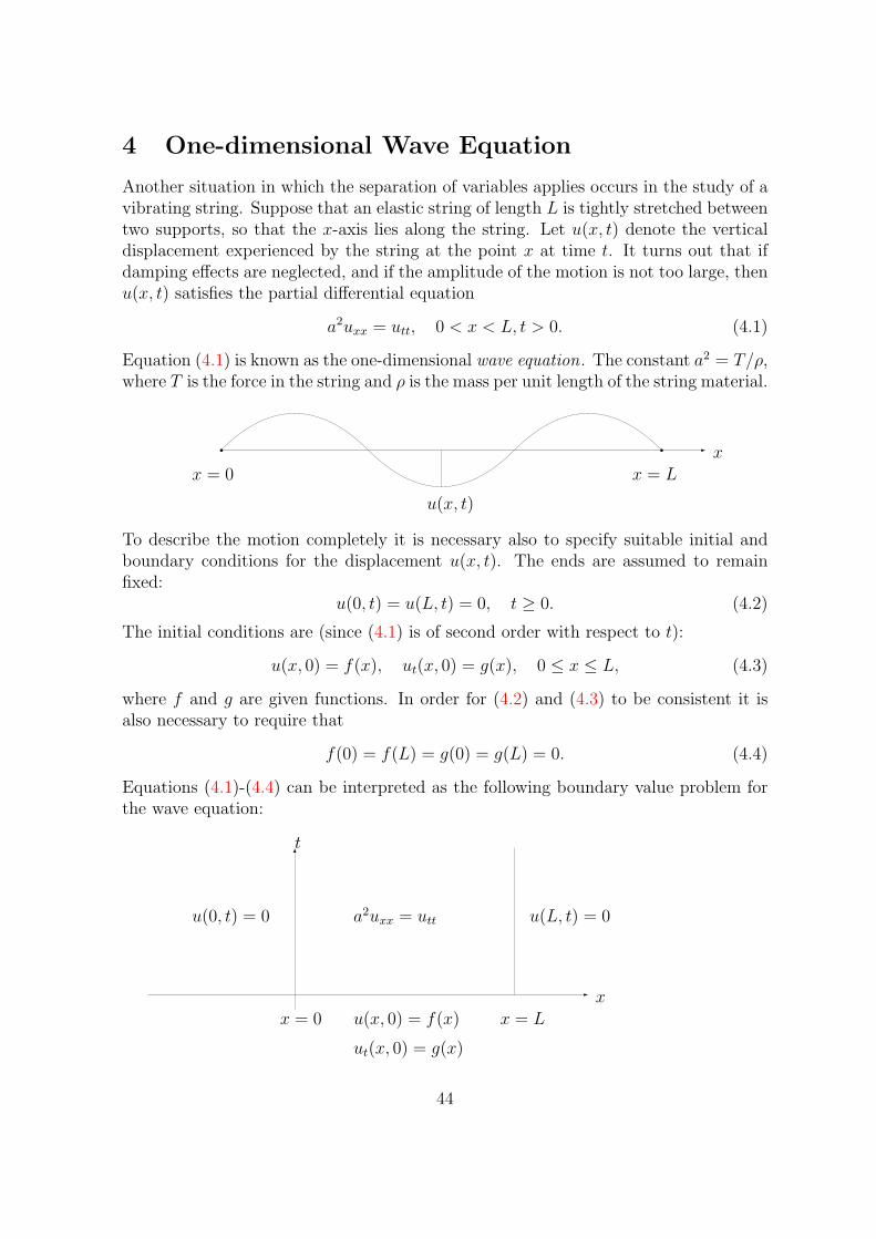
Another situation in which the separation of variables applies occurs in the study of avibrating string. Suppose that an elastic string of length L is tightly stretched betweentwo supports, so that the x-axis lies along the string. Let u(x, t) denote the verticaldisplacement experienced by the string at the point x at time t. It turns out that ifdamping effects are neglected, and if the amplitude of the motion is not too large, thenu(x, t) satisfies the partial differential equation
a2uxx = utt, 0 < x < L, t > 0. (4.1)
Equation (4.1) is known as the one-dimensional wave equation. The constant a2 = T/ρ,where T is the force in the string and ρ is the mass per unit length of the string material.
x
u(x, t)
x = 0 x = L
To describe the motion completely it is necessary also to specify suitable initial andboundary conditions for the displacement u(x, t). The ends are assumed to remainfixed:
u(0, t) = u(L, t) = 0, t ≥ 0. (4.2)
The initial conditions are (since (4.1) is of second order with respect to t):
u(x, 0) = f(x), ut(x, 0) = g(x), 0 ≤ x ≤ L, (4.3)
where f and g are given functions. In order for (4.2) and (4.3) to be consistent it isalso necessary to require that
f(0) = f(L) = g(0) = g(L) = 0. (4.4)
Equations (4.1)-(4.4) can be interpreted as the following boundary value problem forthe wave equation:
xx = 0
t
u(x, 0) = f(x)
ut(x, 0) = g(x)
x = L
u(0, t) = 0 u(L, t) = 0a2uxx = utt
44

Let us apply the method of separation of variables to this homogeneous boundaryvalue problem. Assuming that u(x, t) = X(x)T (t) we obtain
X ′′ + λX = 0, T ′′ + a2λT = 0.
The boundary conditions (4.2) imply that
X ′′ + λX = 0, 0 < x < L
X(0) = X(L) = 0.
This is the same boundary value problem that we have considered before. Hence,
λn =n2π2
L2, Xn(x) = sin
nπx
L, n = 1, 2, . . . .
Taking λ = λn in the equation for T (t) we have
T ′′(t) +(nπaL
)2T (t) = 0.
The general solution to this equation is
T (t) = k1 cosnπat
L+ k2 sin
nπat
L,
where k1 and k2 are arbitrary constants. Using the linear superposition principle weconsider the infinite sum
u(x, t) =∞∑
n=1
sinnπx
L
(an cos
nπat
L+ bn sin
nπat
L
), (4.5)
where the coefficients an and bn are to be determined. It is clear that u(x, t) from (4.5)satisfies (4.1) and (4.2) (at least formally). The initial conditions (4.3) imply
f(x) =∞∑
n=1
an sinnπx
L, 0 ≤ x ≤ L,
g(x) =∞∑
n=1
nπa
Lbn sin
nπx
L, 0 ≤ x ≤ L.
(4.6)
Since (4.4) are fulfilled then (4.6) are the Fourier sine series for f and g, respectively.Therefore,
an =2
L
∫ L
0
f(x) sinnπx
Ldx,
bn =2
nπa
∫ L
0
g(x) sinnπx
Ldx.
(4.7)
45

Finally, we may conclude that the series (4.5) with the coefficients (4.7) solves (at leastformally) the boundary value problem (4.1)-(4.4).
Each displacement pattern
un(x, t) = sinnπx
L
(an cos
nπat
L+ bn sin
nπat
L
)
is called a natural mode of vibration and is periodic in both space variable x and timevariable t. The spatial period 2L
nin x is called the wavelength, while the numbers nπa
L
are called the natural frequencies.
Exercise 18. Find a solution of the problem
uxx = utt, 0 < x < 1, t > 0
u(0, t) = u(1, t) = 0, t ≥ 0
u(x, 0) = x(1− x), ut(x, 0) = sin(7πx)
using the method of separation of variables.
If we compare the two series
u(x, t) =∞∑
n=1
sinnπx
L
(an cos
nπat
L+ bn sin
nπat
L
)
u(x, t) =∞∑
n=1
cn sinnπx
Le−(
nπαL )
2t
for the wave and heat equations we can see that the second series has the exponentialfactor that decays fast with n for any t > 0. This guarantees convergence of the seriesas well as the smoothness of the sum. This is not true anymore for the first seriesbecause it contains only oscillatory terms that do not decay with increasing n.
The boundary value problem for the wave equation with free ends of the string canbe formulated as follows:
a2uxx = utt, 0 < x < L, t > 0
ux(0, t) = ux(L, t) = 0, t ≥ 0
u(x, 0) = f(x), ut(x, 0) = g(x), 0 ≤ x ≤ L.
Let us first note that the boundary conditions imply that f(x) and g(x) must satisfy
f ′(0) = f ′(L) = g′(0) = g′(L) = 0.
The method of separation of variables gives that the eigenvalues are
λn =(nπL
)2, n = 0, 1, 2, . . .
46

and the formal solution u(x, t) is
u(x, t) =b0t+ a0
2+
∞∑
n=1
cosnπx
L
(an cos
nπat
L+ bn sin
nπat
L
).
The initial conditions are satisfied when
f(x) =a02
+∞∑
n=1
an cosnπx
L
and
g(x) =b02+
∞∑
n=1
bnnπa
Lcos
nπx
L,
where
an =2
L
∫ L
0
f(x) cosnπx
Ldx, n = 0, 1, 2, . . .
b0 =2
L
∫ L
0
g(x)dx
and
bn =2
nπa
∫ L
0
g(x) cosnπx
Ldx, n = 1, 2, . . . .
Let us consider the wave equation on the whole line. It corresponds, so to say, tothe infinite string. In that case we no more have the boundary conditions but we havethe initial conditions:
a2uxx = utt,−∞ < x <∞, t > 0
u(x, 0) = f(x), ut(x, 0) = g(x).(4.8)
Proposition. The solution u(x, t) of the wave equation is of the form
u(x, t) = ϕ(x− at) + ψ(x+ at),
where ϕ and ψ are two arbitrary C2 functions of one variable.
Proof. By the chain rule∂ttu− a2∂xxu = 0
if and only if∂ξ∂ηu = 0,
where ξ = x+ at and η = x− at (and so ∂x = ∂ξ + ∂η,1a∂t = ∂ξ − ∂η). It follows that
∂ξu = Ψ(ξ)
oru = ψ(ξ) + ϕ(η),
where ψ′ = Ψ.
47
To satisfy the initial conditions we have
f(x) = ϕ(x) + ψ(x), g(x) = −aϕ′(x) + aψ′(x).
It follows that
ϕ′(x) =1
2f ′(x)− 1
2ag(x), ψ′(x) =
1
2f ′(x) +
1
2ag(x).
Integrating we obtain
ϕ(x) =1
2f(x)− 1
2a
∫ x
0
g(s)ds+ c1, ψ(x) =1
2f(x) +
1
2a
∫ x
0
g(s)ds+ c2,
where c1 and c2 are arbitrary constants. But ϕ(x) + ψ(x) = f(x) implies c1 + c2 = 0.Therefore the solution of the initial value problem is
u(x, t) =1
2(f(x− at) + f(x+ at)) +
1
2a
∫ x+at
x−atg(s)ds. (4.9)
This formula is called the d’Alembert formula.
Exercise 19. Prove that if f is a C2 function and g is a C1 function, then u from(4.9) is a C2 function and satisfies (4.8) in the classical sense.
Exercise 20. Prove that if f and g are merely locally integrable, then u from (4.9) isa distributional solution of (4.8) and the initial conditions are satisfied pointwise.
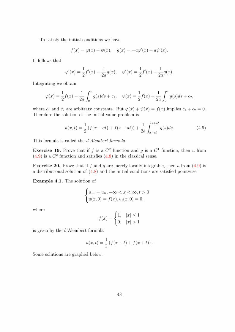
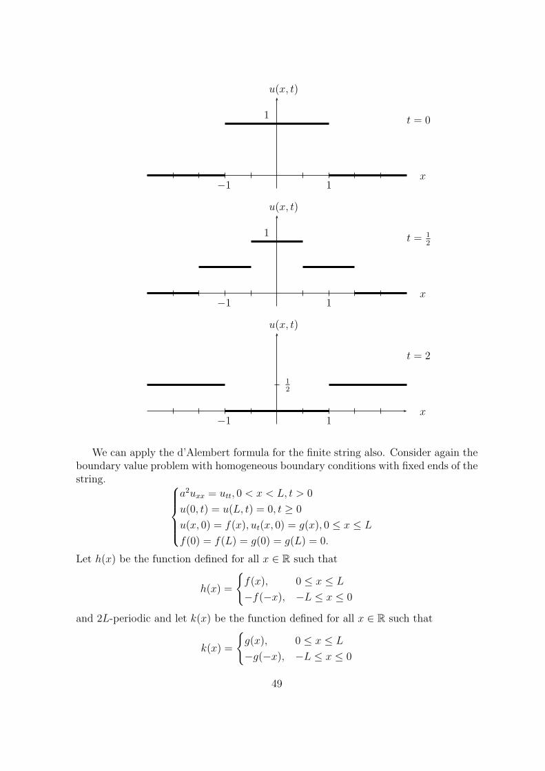
Example 4.1. The solution of
uxx = utt,−∞ < x <∞, t > 0
u(x, 0) = f(x), ut(x, 0) = 0,
where
f(x) =
1, |x| ≤ 1
0, |x| > 1
is given by the d’Alembert formula
u(x, t) =1
2(f(x− t) + f(x+ t)) .
Some solutions are graphed below.
48
x
u(x, t)
t = 0
1−1
1
x
u(x, t)
t = 12
1−1
1
x
u(x, t)
t = 2
1−1
12
We can apply the d’Alembert formula for the finite string also. Consider again theboundary value problem with homogeneous boundary conditions with fixed ends of thestring.
a2uxx = utt, 0 < x < L, t > 0
u(0, t) = u(L, t) = 0, t ≥ 0
u(x, 0) = f(x), ut(x, 0) = g(x), 0 ≤ x ≤ L
f(0) = f(L) = g(0) = g(L) = 0.
Let h(x) be the function defined for all x ∈ R such that
h(x) =
f(x), 0 ≤ x ≤ L
−f(−x), −L ≤ x ≤ 0
and 2L-periodic and let k(x) be the function defined for all x ∈ R such that
k(x) =
g(x), 0 ≤ x ≤ L
−g(−x), −L ≤ x ≤ 0
49

and 2L-periodic. Let us also assume that f and g are C2 functions on the interval[0, L]. Then the solution to the boundary value problem is given by the d’Alembertformula
u(x, t) =1
2(h(x− at) + h(x+ at)) +
1
2a
∫ x+at
x−atk(s)ds.
Remark. It can be checked that this solution is equivalent to the solution which is givenby the Fourier series.
50

5 Laplace Equation in Rectangle and in Disk
One of the most important of all partial differential equations in applied mathematicsis the Laplace equation:
uxx + uyy = 0 2D-equation
uxx + uyy + uzz = 0 3D-equation(5.1)
The Laplace equation appears quite naturally in many applications. For example, asteady state solution of the heat equation in two space dimensions
α2(uxx + uyy) = ut
satisfies the 2D-Laplace equation (5.1). When considering electrostatic fields, the elec-tric potential function must satisfy either 2D or 3D equation (5.1).
A typical boundary value problem for the Laplace equation is (in dimension two):uxx + uyy = 0, (x, y) ∈ Ω ⊂ R2
u(x, y) = f(x, y), (x, y) ∈ ∂Ω,(5.2)
where f is a given function on the boundary ∂Ω of the domain Ω. The problem (5.2)is called the Dirichlet problem (Dirichlet boundary conditions). The problem
uxx + uyy = 0, (x, y) ∈ Ω∂u∂ν(x, y) = g(x, y), (x, y) ∈ ∂Ω,
where g is given and ∂u∂ν
is the outward normal derivative is called the Neumann problem(Neumann boundary conditions).
x
y
Ω
∂Ω
ν |ν| = 1
Dirichlet problem for a rectangle
Consider the boundary value problem in most general form:
wxx + wyy = 0, 0 < x < a, 0 < y < b
w(x, 0) = g1(x), w(x, b) = f1(x), 0 < x < a
w(0, y) = g2(y), w(a, y) = f2(y), 0 ≤ y ≤ b,
51

for fixed a > 0 and b > 0. The solution of this problem can be reduced to the solutionsof
uxx + uyy = 0, 0 < x < a, 0 < y < b
u(x, 0) = u(x, b) = 0, 0 < x < a
u(0, y) = g(y), u(a, y) = f(y), 0 ≤ y ≤ b,
(5.3)
and
uxx + uyy = 0, 0 < x < a, 0 < y < b
u(x, 0) = g1(x), u(x, b) = f1(x), 0 < x < a
u(0, y) = 0, u(a, y) = 0, 0 ≤ y ≤ b.
Due to symmetry in x and y we consider (5.3) only.
x
y
Ω
a
bu(x, b) = 0
u(x, 0) = 0
u(0, y) = g(y) u(a, y) = f(y)
The method of separation of variables gives for u(x, y) = X(x)Y (y),
Y ′′ + λY = 0, 0 < y < b,
Y (0) = Y (b) = 0,(5.4)
andX ′′ − λX = 0, 0 < x < a. (5.5)
From (5.4) one obtains the eigenvalues and eigenfunctions
λn =(nπb
)2, Yn(y) = sin
nπy
b, n = 1, 2, . . . .
Substitute λn into (5.5) to get the general solution
X(x) = c1 coshnπx
b+ c2 sinh
nπx
b.
As above, represent the solution to (5.3) in the form
u(x, y) =∞∑
n=1
sinnπy
b
(an cosh
nπx
b+ bn sinh
nπx
b
). (5.6)
52

The boundary condition at x = 0 gives
g(y) =∞∑
n=1
an sinnπy
b,
with
an =2
b
∫ b
0
g(y) sinnπy
bdy.
At x = a we obtain
f(y) =∞∑
n=1
sinnπy
b
(an cosh
nπa
b+ bn sinh
nπa
b
).
It is a Fourier sine series for f(y). Hence,
an coshnπa
b+ bn sinh
nπa
b=
2
b
∫ b
0
f(y) sinnπy
bdy := bn.
It implies
bn =bn − an cosh
nπab
sinh nπab
. (5.7)
Substituting (5.7) into (5.6) gives
u(x, y) =∞∑
n=1
sinnπy
b
(an cosh
nπx
b+bn − an cosh
nπab
sinh nπab
sinhnπx
b
)
=∞∑
n=1
sinnπy
bbnsinh nπx
b
sinh nπab
+∞∑
n=1
sinnπy
ban
(cosh nπx
bsinh nπa
b− cosh nπa
bsinh nπx
b
sinh nπab
)
=∞∑
n=1
sinnπy
bbnsinh nπx
b
sinh nπab
+∞∑
n=1
sinnπy
ban
sinh nπ(a−x)b
sinh nπab
,
because coshα sinh β − sinhα cosh β = sinh(β − α).
Exercise 21. Find a solution of the problem
uxx + uyy = 0, 0 < x < 2, 0 < y < 1
u(x, 0) = u(x, 1) = 0, 0 < x < 2
u(0, y) = 0, u(2, y) = y(1− y), 0 ≤ y ≤ 1
using the method of separation of variables.
53

Dirichlet problem for a disk
Consider the problem of solving the Laplace equation in a disk x ∈ R2 : |x| < asubject to boundary condition
u(a, θ) = f(θ), (5.8)
where f is a given function on 0 ≤ θ ≤ 2π. In polar coordinates x = r cos θ, y = r sin θ,the Laplace equation takes the form
urr +1
rur +
1
r2uθθ = 0. (5.9)
We apply again the method of separation of variables and assume that
u(r, θ) = R(r)T (θ). (5.10)
Substitution for u in (5.9) yields
R′′T +1
rR′T +
1
r2RT ′′ = 0
or r2R′′ + rR′ − λR = 0
T ′′ + λT = 0.
There are no homogeneous boundary conditions, however we need T (θ) to be 2π-periodic and also bounded. This fact, in particular, leads to
T (0) = T (2π), T ′(0) = T ′(2π). (5.11)
It is possible to show that (5.11) require λ to be real. In what follows we will considerthe three possible cases.
If λ = −µ2 < 0, µ > 0, then the equation for T becomes T ′′ − µ2T = 0 andconsequently
T (θ) = c1eµθ + c2e
−µθ.
It follows from (5.11) that
c1 + c2 = c1e
2πµ + c2e−2πµ
c1 − c2 = c1e2πµ − c2e
−2πµ
so that c1 = c2 = 0.If λ = 0 then T ′′ = 0 and T (θ) = c1 + c2θ. The first condition in (5.11) implies
then that c2 = 0 and therefore T (θ) ≡ constant.If λ = µ2 > 0, µ > 0, then
T (θ) = c1 cos(µθ) + c2 sin(µθ).
54

Now the conditions (5.11) imply thatc1 = c1 cos(2πµ) + c2 sin(2πµ)
c2 = −c1 sin(2πµ) + c2 cos(2πµ)
or c1 sin
2(µπ) = c2 sin(µπ) cos(µπ)
c2 sin2(µπ) = −c1 sin(µπ) cos(µπ).
If sin(µπ) 6= 0 then c1 = c2 cot(µπ)
c2 = −c1 cot(µπ).Hence c21 + c22 = 0 i.e. c1 = c2 = 0. Thus we must have sin(µπ) = 0 and so
λn = n2, Tn(θ) = c1 cos(nθ) + c2 sin(nθ), n = 0, 1, 2, . . . . (5.12)
Turning now to R, for λ = 0 we have r2R′′ + rR′ = 0 i.e. R(r) = k1 + k2 log r. Sincelog r → −∞ as r → 0 we must choose k2 = 0 in order for R (and u) to be bounded.That’s why
R0(r) ≡ constant. (5.13)
For λ = µ2 = n2 the equation for R becomes
r2R′′ + rR′ − n2R = 0.
HenceR(r) = k1r
n + k2r−n.
Again, we must choose k2 = 0 and therefore
Rn(r) = k1rn, n = 1, 2, . . . . (5.14)
Combining (5.10),(5.12), (5.13) and (5.14) we obtain
u(r, θ) =a02
+∞∑
n=1
rn(an cos(nθ) + bn sin(nθ)). (5.15)
The boundary condition (5.8) then requires
u(a, θ) =a02
+∞∑
n=1
an(an cos(nθ) + bn sin(nθ)) = f(θ).
Hence the coefficients are given by
a0 =1
π
∫ 2π
0
f(θ)dθ,
an =1
πan
∫ 2π
0
f(θ) cos(nθ)dθ
55

and
bn =1
πan
∫ 2π
0
f(θ) sin(nθ)dθ.
This procedure can be used also to study the Neumann problem, i.e. the problemin the disk with the boundary condition
∂u
∂r(a, θ) = f(θ). (5.16)
Also in this case the solution u(r, θ) has the form (5.15). The boundary condition(5.16) implies that
∂u
∂r(r, θ)
∣∣∣∣r=a
=∞∑
n=1
nan−1(an cos(nθ) + bn sin(nθ)) = f(θ).
Hence
an =1
πnan−1
∫ 2π
0
f(θ) cos(nθ)dθ
and
bn =1
πnan−1
∫ 2π
0
f(θ) sin(nθ)dθ.
Remark. For the Neumann problem a solution is defined up to an arbitrary constanta02. Moreover, f must satisfy the consistency condition
∫ 2π
0
f(θ)dθ = 0
since integrating
f(θ) =∞∑
n=1
nan−1(an cos(nθ) + bn sin(nθ))
termwise gives us zero.
56

6 The Laplace Operator
We consider what is perhaps the most important of all partial differential operators,the Laplace operator (Laplacian) on Rn, defined by
∆ =n∑
j=1
∂2j ≡ ∇ · ∇.
We will start with a quite general fact about partial differential operators.
Definition. 1. A linear transformation T on Rn is called a rotation if T ′ = T−1.
2. Let h be a fixed vector in Rn. The transformation Thf(x) := f(x + h) is calleda translation.
Theorem 1. Suppose that L is a linear partial differential operator on Rn. Then Lcommutes with translations and rotations if and only if L is a polynomial in ∆, thatis, L ≡∑m
j=0 aj∆j.
Proof. Let
L(x, ∂) ≡∑
|α|≤kaα(x)∂
α
commute with a translation Th. Then
∑
|α|≤kaα(x)∂
αf(x+ h) =∑
|α|≤kaα(x+ h)∂αf(x+ h).
This implies that aα(x) must be constants (because aα(x) ≡ aα(x + h) for all h), sayaα. Next, since L now has constant coefficients we have (see Exercise 5)
Lu(ξ) = P (ξ)u(ξ),
where the polynomial P (ξ) is defined by
P (ξ) =∑
|α|≤kaα(iξ)
α.
Recall from Exercise 4 that if T is a rotation then
u T (ξ) = (u T ) (ξ).
Therefore(Lu)(Tx)(ξ) = Lu(Tξ)
orP (ξ)u(Tx)(ξ) = P (Tξ)u(Tξ).
57
This forcesP (ξ) = P (Tξ).
Write ξ = |ξ|θ, where θ ∈ Sn−1 = x ∈ Rn : |x| = 1 is the direction of ξ. ThenTξ = |ξ|θ′ with some θ′ ∈ Sn−1. But
0 = P (ξ)− P (Tξ) = P (|ξ|θ)− P (|ξ|θ′)shows that P (ξ) does not depend on the angle θ of ξ. Therefore P (ξ) is radial, that is,
P (ξ) = P1(|ξ|) =∑
|α|≤ka′α|ξ||α|.
But since we know that P (ξ) is a polynomial then |α| must be even:
P (ξ) =∑
j
aj|ξ|2j .
By Exercise 5 we have that∆u(ξ) = −|ξ|2u(ξ).
It follows by induction that
∆ju(ξ) = (−1)j|ξ|2ju(ξ), j = 0, 1, . . . .
Taking the inverse Fourier transform we obtain
Lu = F−1(P (ξ)u(ξ)) = F−1∑
j
aj|ξ|2ju(ξ) = F−1∑
j
a′j∆ju(ξ) =
∑
j
a′j∆ju.
Conversely, let
Lu =∑
j
aj∆ju.
It is clear by the chain rule that Laplacian commutes with a translation Th and arotation T . By induction the same is true for any power of ∆ and so for L as well.
Lemma 1. If f(x) = ϕ(r), r = |x|, that is, f is radial, then ∆f = ϕ′′(r) + n−1rϕ′(r).
Proof. Since ∂r∂xj
=xjrthen
∆f =n∑
j=1
∂j(∂jϕ(r)) =n∑
j=1
∂j
(xjrϕ′(r)
)
=n∑
j=1
ϕ′(r)∂j
(xjr
)+
n∑
j=1
x2jr2ϕ′′(r)
=n∑
j=1
(1
r− x2jr3
)ϕ′(r) +
n∑
j=1
x2jr2ϕ′′(r)
=n
rϕ′(r)− 1
r3
n∑
j=1
x2jϕ′(r) + ϕ′′(r) = ϕ′′(r) +
n− 1
rϕ′(r).
58

Corollary. If f(x) = ϕ(r) then ∆f = 0 on Rn\ 0 if and only if
ϕ(r) =
a+ br2−n, n 6= 2
a+ b log r, n = 2,
where a and b are arbitrary constants.
Proof. If ∆f = 0 then by Lemma 1 we have
ϕ′′(r) +n− 1
rϕ′(r) = 0.
Denote ψ(r) := ϕ′(r). Since ψ solves the first order differential equation
ψ′(r) +n− 1
rψ(r) = 0
it can be found by the use of integrating factor. Indeed, multiply by e(n−1) log r = rn−1
to getrn−1ψ′(r) + (n− 1)rn−2ψ(r) = 0
or (rn−1ψ(r)
)′= 0.
It follows thatϕ′(r) = ψ(r) = cr1−n.
Integrate once more to arrive at
ϕ(r) =
cr2−n
2−n + c1, n 6= 2
c log r + c1, n = 2=
ar + b, n = 1
a log r + b, n = 2
ar2−n + b, n ≥ 3.
In the opposite direction the result follows from elementary differentiation.
Definition. A C2 function u on an open set Ω ⊂ Rn is said to be harmonic on Ω if∆u = 0 on Ω.
Exercise 22. For u, v ∈ C2(Ω) ∩ C1(Ω) and for S = ∂Ω, which is a surface of classC1, prove the following Green’s identities :
a) ∫
Ω
(v∆u− u∆v) dx =
∫
S
(v∂νu− u∂νv) dσ
b) ∫
Ω
(v∆u+∇v · ∇u) dx =
∫
S
v∂νudσ.
59

Exercise 23. Prove that if u is harmonic on Ω and u ∈ C1(Ω) then∫
S
∂νudσ = 0.
Corollary (from Green’s identities). If u ∈ C1(Ω) is harmonic on Ω and
1. u = 0 on S, then u ≡ 0
2. ∂νu = 0 on S, then u ≡ constant.
Proof. By resorting to real and imaginary parts it suffices to consider real-valued func-tions. If we let u = v in part b) of Exercise 22 we obtain
∫
Ω
|∇u|2dx =
∫
S
u∂νudσ(x).
In the case 1) we get ∇u ≡ 0 or u ≡ constant. But u ≡ 0 on S implies that u ≡ 0. Inthe case 2) we can conclude only that u ≡ constant.
Theorem 2 (Themean value theorem). Suppose u is harmonic on an open set Ω ⊂ Rn.If x ∈ Ω and r > 0 is small enough so that Br(x) ⊂ Ω, then
u(x) =1
rn−1ωn
∫
|x−y|=ru(y)dσ(y) ≡ 1
ωn
∫
|y|=1
u(x+ ry)dσ(y),
where ωn = 2πn/2
Γ(n/2)is the area of the unit sphere in Rn.
Proof. Let us apply Green’s identity a) with u and v = |y|2−n, if n 6= 2 and v = log |y|if n = 2 in the domain
Br(x)\Bε(x) = y ∈ Rn : ε < |x− y| < r .
Then for v(y − x) we obtain (n 6= 2)
0 =
∫
Br(x)\Bε(x)
(v∆u− u∆v)dy
=
∫
|x−y|=r(v∂νu− u∂νv)dσ(y)−
∫
|x−y|=ε(v∂νu− u∂νv)dσ(y)
= r2−n∫
|x−y|=r∂νudσ(y)− (2− n)r1−n
∫
|x−y|=rudσ(y)
− ε2−n∫
|x−y|=ε∂νudσ(y) + (2− n)ε1−n
∫
|x−y|=εudσ(y). (6.1)
In order to get (6.1) we took into account that
∂ν = ν · ∇ =x− y
r
x− y
r
d
dr=
d
dr
60

for the sphere. Since u is harmonic then due to Exercise 23 we can get from (6.1) thatfor any ε > 0, ε < r,
ε1−n∫
|x−y|=εudσ(y) = r1−n
∫
|x−y|=rudσ(y).
That’s why
limε→0
ε1−n∫
|x−y|=εu(y)dσ(y) = lim
ε→0
∫
|θ|=1
u(x+ εθ)dθ
= ωnu(x) = r1−n∫
|x−y|=ru(y)dσ(y).
This proves the theorem because the latter steps hold for n = 2 also.
Corollary. If u and r are as in Theorem 2 then
u(x) =n
rnωn
∫
|x−y|≤ru(y)dy ≡ n
ωn
∫
|y|≤1
u(x+ ry)dy, x ∈ Ω. (6.2)
Proof. Perform integration in polar coordinates and apply Theorem 2.
Remark. It follows from the latter formula that
vol y : |y| ≤ 1 =ωnn.
Exercise 24. Assume that u is harmonic in Ω. Let χ(x) ∈ C∞0 (B1(0)) be such that
χ(x) = χ1(|x|) and∫Rn χ(x)dx = 1. Define an approximation to the identity by
χε(·) = ε−nχ(ε−1·). Prove that
u(x) =
∫
Bε(x)
χε(x− y)u(y)dy
for x ∈ Ωε := x ∈ Ω : Bε(x) ⊂ Ω.
Corollary 1. If u is harmonic on Ω then u ∈ C∞(Ω).
Proof. The statement follows from Excercise 24 since the function χε is compactlysupported and we may thus differentiate under the integral sign as often as we please.
Corollary 2. If uk∞k=1 is a sequence of harmonic functions on an open set Ω ⊂ Rn
which converges uniformly on compact subsets of Ω to a limit u, then u is harmonicon Ω.
Theorem 3 (The maximum principle). Suppose Ω ⊂ Rn is open and connected. If uis real-valued and harmonic on Ω with supx∈Ω u(x) = A < ∞, then either u < A forall x ∈ Ω or u(x) ≡ A in Ω.
61

Proof. Since u is continuous on Ω then the set x ∈ Ω : u(x) = A is closed in Ω. Onthe other hand due to Theorem 2 (see (6.2)) we may conclude that if u(x) = A insome point x ∈ Ω then u(y) = A for all y in a ball about x. Indeed, if y0 ∈ B′
σ(x) andu(y0) < A then u(y) < A for all y from small neighborhood of y0. Hence, by Corollaryof Theorem 2,
u(x) =n
rnωn
∫
|x−y|≤ru(y)dy
=n
rnωn
∫
|x−y|≤r,|y0−y|>εu(y)dy +
n
rnωn
∫
|y−y0|≤εu(y)dy
< A
(n
rnωn
∫
|x−y|≤r,|y0−y|>εdy +
n
rnωn
∫
|y−y0|≤εdy
)
= An
rnωn
∫
|x−y|≤rdy = A,
that is, A < A. This contradiction proves our statement. This fact also means thatthe set x ∈ Ω : u(x) = A is also open. Hence it is either Ω (in this case u ≡ A in Ω)or the empty set (in this case u(x) < A in Ω).
Corollary 1. Suppose Ω ⊂ Rn is open and bounded. If u is real-valued and harmonicon Ω and continuous on Ω, then the maximum and minimum of u on Ω are achievedonly on ∂Ω.
Corollary 2 (The uniqueness theorem). Suppose Ω is as in Corollary 1. If u1 andu2 are harmonic on Ω and continuous in Ω (might be complex-valued) and u1 = u2 on∂Ω, then u1 = u2 on Ω.
Proof. The real and imaginary parts of u1 − u2 and u2 − u1 are harmonic on Ω. Hencethey must achieve their maximum on ∂Ω. These maximum are, therefore zero, sou1 ≡ u2.
Theorem 4 (Liouville’s theorem). If u is bounded and harmonic on Rn then u ≡constant.
Proof. For any x ∈ Rn and |x| ≤ R by Corollary of Theorem 2 we have
|u(x)− u(0)| = n
Rnωn
∣∣∣∣∫
BR(x)
u(y)dy −∫
BR(0)
u(y)dy
∣∣∣∣ ≤n
Rnωn
∫
D
|u(y)|dy,
whereD = (BR(x)\BR(0)) ∪ (BR(0)\BR(x))
is the symmetric difference of the balls BR(x) and BR(0). That’s why we obtain
|u(x)− u(0)| ≤ n ‖u‖∞Rnωn
∫
R−|x|≤|y|≤R+|x|dy ≤ n ‖u‖∞
Rnωn
∫ R+|x|
R−|x|rn−1dr
∫
|θ|=1
dθ
=(R + |x|)n − (R− |x|)n
Rn‖u‖∞ = O
(1
R
)‖u‖∞ .
Hence the difference |u(x)− u(0)| vanishes as R → ∞, that is, u(x) = u(0).
62

Definition. A fundamental solution for a partial differential operator L is a distribu-tion K ∈ D′ such that
LK = δ.
Remark. Note that a fundamental solution is not unique. Any two fundamental solu-tions differ by a solution of the homogeneous equation Lu = 0.
Exercise 25. Show that the characteristic function of the set(x1, x2) ∈ R2 : x1 > 0, x2 > 0
is a fundamental solution for L = ∂1∂2.
Exercise 26. Prove that the Fourier transform of 1x1+ix2
in R2 is equal to − iξ1+iξ2
.
Exercise 27. Show that the fundamental solution for the Cauchy-Riemann operatorL = 1
2(∂1 + i∂2) on R2 is equal to
1
π
1
x1 + ix2.
Since the Laplacian commutes with rotations (Theorem 1) it should have a radialfundamental solution which must be a function of |x| that is harmonic on Rn\ 0.Theorem 5. Let
K(x) =
|x|2−n
(2−n)ωn, n 6= 2
12π
log |x|, n = 2.(6.3)
Then K is a fundamental solution for ∆.
Proof. For ε > 0 we consider a smoothed out version Kε of K as
Kε(x) =
(|x|2+ε2)
2−n2
(2−n)ωn, n 6= 2
14π
log(|x|2 + ε2), n = 2.(6.4)
Then Kε → K pointwise (x 6= 0) as ε → +0 and Kε and K are dominated by a fixedlocally integrable function for ε ≤ 1 (namely, by |K| for n > 2, | log |x|| + 1 for n = 2and (|x|2 + 1)1/2 for n = 1). So by the Lebesgue’s dominated convergence theoremKε → K in L1
loc (or in the topology of distributions) when ε→ +0. Hence we need toshow only that ∆Kε → δ as ε→ 0 in the sense of distributions, that is,
〈∆Kε, ϕ〉 → ϕ(0), ε→ 0
for any ϕ ∈ C∞0 (Rn).
Exercise 28. Prove that
∆Kε(x) = nω−1n ε2(|x|2 + ε2)−(
n2+1) ≡ ε−nψ(ε−1x)
for ψ(y) = nω−1n (|y|2 + 1)−(
n2+1).
63
Exercise 28 allows us to write
〈∆Kε, ϕ〉 =
∫
Rn
ϕ(x)ε−nψ(ε−1x)dx =
∫
Rn
ϕ(εz)ψ(z)dz → ϕ(0)
∫
Rn
ψ(z)dz
as ε→ +0. So it remains to show that∫
Rn
ψ(z)dz = 1.
Using Exercise 28 we have
∫
Rn
ψ(x)dx =n
ωn
∫
Rn
(|x|2 + 1)−(n2+1)dx =
n
ωn
∫ ∞
0
rn−1(r2 + 1)−(n2+1)dr
∫
|θ|=1
dθ
= n
∫ ∞
0
rn−1(r2 + 1)−(n2+1)dr =
n
2
∫ ∞
0
t(n−1)/2(1 + t)−n2−1 1√
tdt
=n
2
∫ ∞
0
tn/2−1(1 + t)−n2−1dt =
n
2
∫ 1
0
(1
s− 1
)n/2−1
sn2+1ds
s2
=n
2
∫ 1
0
(1− s)n/2−1 ds =n
2
∫ 1
0
τn/2−1dτ = 1.
It means that ε−1ψ(ε−1x) is an approximation to the identity and
∆Kε → δ.
But Kε → K and so ∆K = δ also.
Theorem 6. Suppose that
1. f ∈ L1(Rn) if n ≥ 3
2.∫R2 |f(y)| (| log |y||+ 1) dy <∞ if n = 2
3.∫R|f(y)| (1 + |y|) dy <∞ if n = 1.
Let K be given by (6.3). Then f ∗K is well-defined as a locally integrable function and∆(f ∗K) = f in the sense of distributions.
Proof. Let n ≥ 3 and set
χ1(x) =
1, x ∈ B1(0)
0, x /∈ B1(0).
Then χ1K ∈ L1(Rn) and (1 − χ1)K ∈ L∞(Rn). So, for f ∈ L1(Rn) we have thatf ∗ (χ1K) ∈ L1(Rn) and f ∗ (1 − χ1)K ∈ L∞(Rn) (see Proposition 1 of Chapter 0).
64

Hence f ∗K ∈ L1loc(R
n) by addition and we may calculate
〈∆(f ∗K), ϕ〉 = 〈f ∗K,∆ϕ〉, ϕ ∈ C∞0 (Rn)
=
∫
Rn
(f ∗K)(x)∆ϕ(x)dx =
∫
Rn
∫
Rn
f(y)K(x− y)dy∆ϕ(x)dx
=
∫
Rn
f(y)
∫
Rn
K(x− y)∆ϕ(x)dxdy =
∫
Rn
f(y)〈K(x− y),∆ϕ(x)〉dy
=
∫
Rn
f(y)〈∆K(x− y), ϕ(x)〉dy =
∫
Rn
f(y)〈δ(x− y), ϕ(x)〉dy
=
∫
Rn
f(y)ϕ(y)dy = 〈f, ϕ〉.
Hence ∆(f ∗K) = f .
Exercise 29. Prove Theorem 6 for n = 2.
Exercise 30. Prove Theorem 6 for n = 1.
Theorem 7. Let Ω be a bounded domain in Rn (for n = 1 assume that Ω = (a, b))with C1 boundary ∂Ω = S. If u ∈ C1(Ω) is harmonic in Ω, then
u(x) =
∫
S
(u(y)∂νyK(x− y)−K(x− y)∂νu(y)
)dσ(y), x ∈ Ω, (6.5)
where K(x) is the fundamental solution (6.3).
Proof. Let us consider Kε from (6.4). Then since ∆u = 0 in Ω, by Green’s identity a)(see Exercise 22) we have
∫
Ω
u(y)∆yKε(x− y)dy =
∫
S
(u(y)∂νyKε(x− y)−Kε(x− y)∂νu(y)
)dσ(y).
As ε → 0 the right hand side of this equation tends to the right hand side of (6.5)for each x ∈ Ω. This is because for x ∈ Ω and y ∈ S there are no singularities in K.On the other hand, the left hand side is just (u ∗∆Kε) (x) if we set u ≡ 0 outside Ω.According to the proof of Theorem 5
(u ∗∆Kε) (x) → u(x), ε→ 0,
completing the proof.
Remark. If we know that u = f and ∂νu = g on S then
u(x) =
∫
S
(f(y)∂νyK(x− y)−K(x− y)g(y)
)dσ(y)
is the solution of ∆u = 0 with Cauchy data on S. But this problem is overdeterminedbecause we know from Corollary 2 of Theorem 3 that the solution of ∆u = 0 is uniquelydetermined by f alone.
65

The following theorem concerns spaces Cα(Ω) and Ck,α(Ω) which are defined by
Cα(Ω) ≡ C0,α(Ω) = u ∈ L∞(Ω) : |u(x)− u(y)| ≤ C|x− y|α, x, y ∈ ΩCk,α(Ω) ≡ Ck+α(Ω) =
u : ∂βu ∈ Cα(Ω), |β| ≤ k
for 0 < α < 1 and k ∈ N.
Theorem 8. Suppose k ≥ 0 is an integer, 0 < α < 1 and Ω ⊂ Rn open. If f ∈ Ck+α(Ω)and u is a distributional solution of ∆u = f in Ω, then u ∈ Ck+2+α
loc (Ω).
Proof. Since ∆(∂βu) = ∂β∆u = ∂βf we can assume without loss of generality thatk = 0. Given Ω1 ⊂ Ω such that Ω1 ⊂ Ω pick ϕ ∈ C∞
0 (Ω) such that ϕ ≡ 1 on Ω1 andlet g = ϕf .
Since ∆(g ∗ K) = g (see Theorem 6) and therefore ∆(g ∗ K) = f in Ω1, thenu − (g ∗ K) is harmonic in Ω1 and hence C∞ there. It is therefore enough to provethat if g is a Cα function with compact support, then g ∗ K ∈ C2+α. To this endwe consider Kε(x) and its derivatives. Straightforward calculations lead to followingformulae (n ≥ 1):
∂
∂xjKε(x) = ω−1
n xj(|x|2 + ε2)−n/2
∂2
∂xi∂xjKε(x) = ω−1
n
−nxixj(|x|2 + ε2)−n/2−1, i 6= j
(|x|2 + ε2 − nx2j)(|x|2 + ε2)−n/2−1, i = j.
(6.6)
Exercise 31. Prove formulae (6.6).
Since Kε ∈ C∞ then g ∗ Kε ∈ C∞ also. Moreover, ∂j(g ∗ Kε) = g ∗ ∂jKε and∂i∂j(g ∗Kε) = g ∗ ∂i∂jKε. The pointwise limits in (6.6) as ε→ 0 imply
∂
∂xjK(x) = ω−1
n xj|x|−n
∂2
∂xi∂xjK(x) =
−nω−1
n xixj|x|−n−2, i 6= j
ω−1n (|x|2 − nx2j)|x|−n−2, i = j,
(6.7)
for x 6= 0. The formulae (6.7) show that ∂jK(x) is a locally integrable functionand since g is bounded with compact support then g ∗ ∂jK is continuous. Next,g ∗ ∂jKε → g ∗ ∂jK uniformly as ε → +0. It is equivalent to ∂jKε → ∂jK in thetopology of distributions (see the definition). Hence ∂j(g ∗K) = g ∗ ∂jK.
This argument does not work for the second derivatives because ∂i∂jK(x) is notintegrable. But there is a different procedure for these terms.
Let i 6= j. Then ∂i∂jKε(x) and ∂i∂jK(x) are odd functions of xi (and xj), see (6.6)and (6.7). Due to this fact their integrals over any annulus 0 < a < |x| < b vanish.For Kε we can even take a = 0.
Exercise 32. Prove this fact.
66

That’s why for any b > 0 we have
g ∗ ∂i∂jKε(x) =
∫
Rn
g(x− y)∂i∂jKε(y)dy − g(x)
∫
|y|<b∂i∂jKε(y)dy
=
∫
|y|<b(g(x− y)− g(x))∂i∂jKε(y)dy +
∫
|y|≥bg(x− y)∂i∂jKε(y)dy.
If we let ε→ 0 we obtain
limε→0
g ∗ ∂i∂jKε(x) =
∫
|y|<b(g(x− y)− g(x))∂i∂jK(y)dy +
∫
|y|≥bg(x− y)∂i∂jK(y)dy.
This limit exists because
|g(x− y)− g(x)||∂i∂jK(y)| ≤ c|y|α|y|−n
(g is Cα) and because g is compactly supported. Then, since b is arbitrary, we can letb→ +∞ to obtain
∂i∂j(g ∗K)(x) = limb→∞
∫
|y|<b(g(x− y)− g(x))∂i∂jK(y)dy
+ limb→∞
∫
|y|≥bg(x− y)∂i∂jK(y)dy
= limb→∞
∫
|y|<b(g(x− y)− g(x))∂i∂jK(y)dy. (6.8)
A similar result holds for i = j. Indeed,
∂2jKε(x) =1
nε−nψ(ε−1x) +Kε
j (x),
where ψ(x) = nω−1n (|x|2 + 1)−n/2−1 and Kε
j = ω−1n (|x|2 − nx2j)(|x|2 + ε2)−n/2−1 (see
(6.6)). The integral Ij of Kεj over an annulus a < |y| < b vanishes. Why is it so? First
of all, Ij is independent of j by symmetry in the coordinates, that is, Ij = Ii for i 6= j.So nIj is the integral of
∑nj=1K
εj . But
∑nj=1K
εj = 0. Hence Ij = 0 also. That’s why
we can apply the same procedure. Since
g ∗ (ε−nψ(ε−1x)) → g, ε→ 0,
(because ε−nψ(ε−1x) is an approximation to the identity) then
∂2j (g ∗K)(x) =g(x)
n+ lim
b→∞
∫
|y|<b(g(x− y)− g(x))∂2jK(y)dy. (6.9)
Since the convergence in (6.8) and (6.9) is uniform then at this point we have shownthat g ∗K ∈ C2. But we need to prove more.
67

Lemma 2 (Calderon-Zigmund). Let N be a C1 function on Rn\ 0 that is homoge-neous of degree −n and satisfies
∫
a<|y|<bN(y)dy = 0
for any 0 < a < b < ∞. Then if g is a Cα function with compact support, 0 < α < 1,then
h(x) = limb→∞
∫
|z|<b(g(x− z)− g(x))N(z)dz
belongs to Cα.
Proof. Let us write h = h1 + h2, where
h1(x) =
∫
|z|≤3|y|(g(x− z)− g(x))N(z)dz,
h2(x) = limb→∞
∫
3|y|<|z|<b(g(x− z)− g(x))N(z)dz.
We wish to estimate h(x+ y)− h(x). Since α > 0 we have
|h1(x)| ≤ c
∫
|z|≤3|y||z|α|z|−ndz = c′|y|α.
and hence|h1(x+ y)− h1(x)| ≤ |h1(x+ y)|+ |h1(x)| ≤ 2c′|y|α.
On the other hand
h2(x+ y)− h2(x) = limb→∞
∫
3|y|<|z+y|<b(g(x− z)− g(x))N(z + y)dz
− limb→∞
∫
3|y|<|z|<b(g(x− z)− g(x))N(z)dz
= limb→∞
∫
3|y|<|z|<b(g(x− z)− g(x))(N(z + y)−N(z))dz
+ limb→∞
∫
3|y|<|z+y|<b\3|y|<|z|<b(g(x− z)− g(x))N(z + y)dz
= I1 + I2.
It is clear that
3|y| < |z + y| \ 3|y| < |z| ⊂ 2|y| < |z| \ 3|y| < |z|= 2|y| < |z| ≤ 3|y| .
68

That’s why
|I2| ≤∫
2|y|<|z|≤3|y||g(x− z)− g(x)||N(z + y)|dz
≤ c
∫
2|y|<|z|≤3|y||z|α|z + y|−ndz
≤ c′∫
2|y|<|z|≤3|y||z|α−ndz = c′′|y|α.
Now we observe that for |z| > 3|y||N(z + y)−N(z)| ≤ |y| sup
0≤t≤1|∇N(z + ty)|
≤ c|y| sup0≤t≤1
|z + ty|−n−1 ≤ c′|y||z|−n−1,
because ∇N is homogeneous of degree −n− 1, since N is homogeneous of degree −n.Hence
|I1| ≤ c
∫
|z|>3|y||z|α|y||z|−n−1dz = c′|y|
∫ ∞
3|y|ρα−2dρ = c′′|y|α.
Note that the condition α < 1 is needed here. Collecting the estimates for I1 and I2we can see that the lemma is proved.
In order to end the proof of Theorem it remains to note that ∂i∂jK(x) satisfies allconditions of Lemma 2. Thus the Theorem is also proved.
Exercise 33. Show that a function K1 is a fundamental solution for ∆2 ≡ ∆(∆) onRn if and only if K1 satisfies the equation
∆K1 = K,
where K is the fundamental solution for the Laplacian.
Exercise 34. Show that the following functions are the fundamental solutions for ∆2
on Rn:
1. n = 4:
− log |x|4ω4
2. n = 2:|x|2 log |x|
8π
3. n 6= 2, 4:|x|4−n
2(4− n)(2− n)ωn.
Exercise 35. Show that (4π|x|)−1e−c|x| is the fundamental solution for −∆+ c2 on R3
for any constant c ∈ C.
69

7 The Dirichlet and Neumann Problems
The Dirichlet problem
Given functions f in Ω and g on S = ∂Ω, find a function u in Ω = Ω ∪ ∂Ω satisfying∆u = f, in Ω
u = g, onS.(D)
The Neumann problem
Given functions f in Ω and g on S, find a function u in Ω satisfying∆u = f, in Ω
∂νu = g, onS.(N)
We assume that Ω is bounded with C1 boundary. But we shall not, however, assumethat Ω is connected. The uniqueness theorem (see Corollary of Theorem 3 of Chapter6) shows that the solution of (D) will be unique (if it exists), at least if we requireu ∈ C(Ω). For (N) uniqueness does not hold: we can add to u(x) any function that isconstant on each connected component of Ω. Moreover, there is an obvious necessarycondition for solvability of (N). If Ω′ is a connected component of Ω then
∫
Ω′
∆udx =
∫
∂Ω′
∂νudσ(x) =
∫
∂Ω′
g(x)dσ(x) =
∫
Ω′
fdx,
that is, ∫
Ω′
f(x)dx =
∫
∂Ω′
g(x)dσ(x).
It is also clear (by linearity) that (D) can be reduced to the following homogeneousproblems:
∆v = f, in Ω
v = 0, onS(DA)
∆w = 0, in Ω
w = g, onS(DB)
and u := v + w solves (D). Similar remarks apply to (N), that is∆v = f, in Ω
∂νv = 0, onS
∆w = 0, in Ω
∂νw = g, onS
and u = v + w.
70

Definition. The Green’s function for (D) in Ω is the solution G(x, y) of the boundaryvalue problem
∆xG(x, y) = δ(x− y), x, y ∈ Ω
G(x, y) = 0, x ∈ S, y ∈ Ω.(7.1)
Analogously, the Green’s function for (N) in Ω is the solution G(x, y) of the boundaryvalue problem
∆xG(x, y) = δ(x− y), x, y ∈ Ω
∂νxG(x, y) = 0, x ∈ S, y ∈ Ω.(7.2)
This definition allows us to write
G(x, y) = K(x− y) + vy(x), (7.3)
where K is the fundamental solution of ∆ in Rn and, for any y ∈ Ω, the function vy(x)satisfies
∆vy(x) = 0, in Ω
vy(x) = −K(x− y), onS(7.4)
in the case of (7.1) and
∆vy(x) = 0, in Ω
∂νxvy(x) = −∂νxK(x− y), onS
in the case of (7.2). Since (7.4) guarantees that vy is real then so is G correspondingto (7.1).
Lemma 1. The Green’s function (7.1) exists and is unique.
Proof. The uniqueness of G follows again from Corollary 2 of Theorem 3 of Chapter6, since K(x− y) in (7.4) is continuous for all x ∈ S and y ∈ Ω (x 6= y). The existencewill be proved later.
Lemma 2. For both (7.1) and (7.2) it is true that G(x, y) = G(y, x) for all x, y ∈ Ω.
Proof. Let G(x, y) and G(x, z) be the Green’s functions for Ω corresponding to sourceslocated at fixed y and z, y 6= z, respectively. Let us consider the domain
Ωε = (Ω\ x : |x− y| < ε) \ x : |x− z| < ε ,
see Figure 2.
71

b
b
y
z
Figure 2: The domain Ωε.
If x ∈ Ωε then x 6= z and x 6= y and, therefore, ∆xG(x, z) = 0 and ∆xG(x, y) = 0.These facts imply
0 =
∫
Ωε
(G(x, y)∆xG(x, z)−G(x, z)∆xG(x, y)) dx
=
∫
S
(G(x, y)∂νxG(x, z)−G(x, z)∂νxG(x, y)) dσ(x)
−∫
|x−y|=ε(G(x, y)∂νxG(x, z)−G(x, z)∂νxG(x, y)) dσ(x)
−∫
|x−z|=ε(G(x, y)∂νxG(x, z)−G(x, z)∂νxG(x, y)) dσ(x).
Hence, by (7.1) or (7.2), for arbitrary ε > 0 (small enough)∫
|x−y|=ε(G(x, y)∂νxG(x, z)−G(x, z)∂νxG(x, y)) dσ(x)
=
∫
|x−z|=ε(G(x, z)∂νxG(x, y)−G(x, y)∂νxG(x, z)) dσ(x).
Let n ≥ 3. Due to (7.3) for ε→ 0 we have∫
|x−y|=ε(G(x, y)∂νxG(x, z)−G(x, z)∂νxG(x, y)) dσ(x)
≈ cn
∫
|x−y|=εε2−n
((2− n)
(x− y, x− z)
|x− y||x− z|n + ∂νxvz(x)
)dσ(x)
−∫
|x−y|=εG(x, z)∂νxG(x, y)dσ(x)
≈ cn(2− n)ε2−nεn−11
ε
∫
θ
(εθ, εθ + y − z)
|εθ + y − z|n dθ − I1 ≈ −I1,
where we have denoted
I1 =
∫
|x−y|=εG(x, z)∂νxG(x, y)dσ(x).
72

The same is true for the integral over |x− z| = ε, that is,
∫
|x−z|=ε(G(x, z)∂νxG(x, y)−G(x, y)∂νxG(x, z)) dσ(x) ≈ −I2, ε→ 0,
where
I2 =
∫
|x−z|=εG(x, y)∂νxG(x, z)dσ(x).
But using the previous techniques we can obtain that
I1 ≈ (2− n)cnε1−nεn−1
∫
|θ|=1
G(εθ + y, z)dθ → (2− n)cnωnG(y, z), ε→ 0
and
I2 ≈ (2− n)cnε1−nεn−1
∫
|θ|=1
G(εθ + z, y)dθ → (2− n)cnωnG(z, y), ε→ 0.
It means that G(y, z) = G(z, y) for all z 6= y. This proof holds for n = 2 (and even forn = 1) with some simple changes.
Lemma 3. In three or more dimensions
K(x− y) < G(x, y) < 0, x, y ∈ Ω, x 6= y
where G(x, y) is the Green’s function for (D).
Proof. For each fixed y, the function vy(x) := G(x, y)−K(x− y) is harmonic in Ω, see(7.4). Moreover, on S = ∂Ω, vy(x) takes on the positive value
−K(x− y) ≡ −|x− y|2−nωn(2− n)
.
By the minimum principle, it follows that vy(x) is strictly positive in Ω. This provesthe first inequality.
Exercise 36. Prove the second inequality in Lemma 3.
Exercise 37. Show that for n = 2 Lemma 3 has the following form:
1
2πlog
|x− y|h
< G(x, y) < 0, x, y ∈ Ω,
where h ≡ maxx,y∈Ω |x− y|.
73

Exercise 38. Obtain the analogue of Lemma 3 for n = 1. Hint: show that the Green’sfunction for the operator d2
dx2on Ω = (0, 1) is
G(x, y) =
x(y − 1), x < y
y(x− 1), x > y.
Remark. G(x, y) may be extended naturally (because of the symmetry) to Ω × Ω bysetting G(x, y) = 0 for y ∈ S.
Now we can solve both problems (DA) and (DB). Indeed, let us set f = 0 in (DA)outside Ω and define
v(x) :=
∫
Ω
G(x, y)f(y)dy ≡ (f ∗K)(x) +
∫
Ω
(G(x, y)−K(x− y)) f(y)dy.
Then the Laplacian of the first term is f (see Theorem 6 of Chapter 6), and the secondterm is harmonic in x (since vy(x) is harmonic). Also v(x) = 0 on S because the sameis true for G. Thus, this v(x) solves (DA).
Consider now (DB). We assume that g is continuous on S and we wish to findw which is continuous on Ω. Applying Green’s identity a) (together with the samelimiting process as in the proof of Lemma 2) we obtain
w(x) =
∫
Ω
(w(y)∆yG(x, y)−G(x, y)∆w(y)) dy
=
∫
S
w(y)∂νyG(x, y)dσ(y) =
∫
S
g(y)∂νyG(x, y)dσ(y).
Let us denote the last integral by (P). Since ∂νyG(x, y) is harmonic in x and continuousin y for x ∈ Ω and y ∈ S then w(x) is harmonic in Ω. In order to prove that this w(x)solves (DB) it remains to prove that w(x) is continuous in Ω and w(x) on S is g(x).We will prove this general fact later.
Definition. The function ∂νyG(x, y) on Ω× S is called the Poisson kernel for Ω and(P) is called the Poisson integral .
Now we are in the position to solve the Dirichlet problem in a half-space. Let
Ω = Rn+1+ =
(x′, xn+1) ∈ Rn+1 : x′ ∈ Rn, xn+1 > 0
,
where n ≥ 1 now, and let xn+1 = t. Then
∆n+1 = ∆n + ∂2t , n = 1, 2, . . .
Denote by K(x, t) a fundamental solution for ∆n+1 in Rn+1, that is,
K(x, t) =
(|x|2+t2)
1−n2
(1−n)ωn+1, n > 1
14π
log(|x|2 + t2), n = 1.
74

Let us prove then that the Green’s function for Rn+1+ is
G(x, y; t, s) = K(x− y, t− s)−K(x− y,−t− s). (7.5)
It is clear (see (7.5)) that G(x, y; t, 0) = G(x, y; 0, s) = 0 and
∆n+1G = δ(x− y, t− s)− δ(x− y,−t− s) = δ(x− y)δ(t− s)
because for t, s > 0,−t− s < 0 and, therefore, δ(−t− s) = 0. Thus G is the DirichletGreen’s function for Rn+1
+ . From this we immediately have the solution of (DA) inRn+1
+ as
u(x, t) =
∫
Rn
∫ ∞
0
G(x, y; t, s)f(y, s)dsdy.
To solve (DB) we compute the Poisson kernel for this case. Since the outward normalderivative on ∂Rn+1
+ is − ∂∂t
then the Poisson kernel becomes
− ∂
∂sG(x, y; t, s)|s=0 = − ∂
∂s(K(x− y, t− s)−K(x− y,−t− s)) |s=0
=2t
ωn+1(|x− y|2 + t2)n+12
. (7.6)
Exercise 39. Prove (7.6).
Note that (7.6) holds for any n ≥ 1. According to the formula for (P), the candidatefor a solution to (DB) is:
u(x, t) =2
ωn+1
∫
Rn
tg(y)
(|x− y|2 + t2)n+12
dy. (7.7)
In other words, if we set
Pt(x) :=2t
ωn+1(|x|2 + t2)n+12
, (7.8)
which is what is usually called the Poisson kernel for Rn+1+ , the proposed solution (7.7)
is simply equal tou(x, t) = (g ∗ Pt)(x). (7.9)
Exercise 40. Prove that Pt(x) = t−nP1(t−1x) and
∫
Rn
Pt(y)dy = 1.
Theorem 1. Suppose g ∈ Lp(Rn), 1 ≤ p ≤ ∞. Then u(x, t) from (7.9) is well-definedon Rn+1
+ and is harmonic there. If g is bounded and uniformly continuous, then u(x, t)
is continuous on Rn+1+ and u(x, 0) = g(x), and
‖u(·, t)− g(·)‖∞ → 0
as t→ +0.
75

Proof. It is clear that for any t > 0, Pt(x) ∈ L1(Rn) ∩ L∞(Rn), see (7.8). HencePt(x) ∈ Lq(Rn) for all q ∈ [1,∞] with respect to x and for any fixed t > 0. Therefore,the integral in (7.9) is absolutely convergent and the same is true if Pt is replaced byits derivatives ∆xPt or ∂
2t Pt (due to Young’s inequality for convolution).
Since G(x, y; t, s) is harmonic for (x, t) 6= (y, s) then Pt(x) is also harmonic and
∆xu+ ∂2t u = g ∗ (∆x + ∂2t )Pt = 0.
It remains to prove that if g is bounded and continuous then
‖u(·, t)− g(·)‖∞ → 0
as t→ +0 and, therefore, u(x, 0) = g(x) and u is continuous on Rn+1+ .
We have (see Exercise 40)
‖g ∗ Pt − g‖∞ = supx∈Rn
∣∣∣∣∫
Rn
g(x− y)Pt(y)dy −∫
Rn
g(x)Pt(y)dy
∣∣∣∣
≤ supx∈Rn
∫
Rn
|g(x− y)− g(x)||Pt(y)|dy
= supx∈Rn
∫
Rn
|g(x− tz)− g(x)||P1(z)|dz
= supx∈Rn
(∫
|z|<R|g(x− tz)− g(x)||P1(z)|dz
+
∫
|z|≥R|g(x− tz)− g(x)||P1(z)|dz
)
≤ supx∈Rn,|z|<R
|g(x− tz)− g(x)|+ 2 ‖g‖∞∫
|z|≥R|P1(z)|dz < ε
for t small enough.The first term in the latter sum can be made less than ε/2 since g is uniformly
continuous on Rn. The second term can be made less than ε/2 for R large enoughsince P1 ∈ L1(Rn). Thus, the theorem is proved.
Remark. The solution of the considered problem is not unique: if u(x, t) is a solutionthen so is u(x, t) + ct for any c ∈ C. However, we have the following theorem.
Theorem 2. If g ∈ C(Rn) and limx→∞ g(x) = 0 then u(x, t) := (g ∗ Pt)(x) → 0 as(x, t) → ∞ in Rn+1
+ and it is the unique solution with this property.
Proof. Assume for the moment that g has compact support, say g = 0 for |x| > R.Then g ∈ L1(Rn) and
‖g ∗ Pt‖∞ ≤ ‖g‖1 ‖Pt‖∞ ≤ ct−n,
so u(x, t) → 0 as t→ ∞ uniformly in x. On the other hand, if 0 < t ≤ T , then
|u(x, t)| ≤ ‖g‖1 sup|y|<R
|Pt(x− y)| = ‖g‖1 sup|y|<R
2t
ωn+1(|x− y|2 + t2)n+12
≤ cT |x|−n−1,
76

for |x| > 2R. Hence u(x, t) → 0 as x → ∞ uniformly for t ∈ [0, T ]. This provesthat u(x, t) vanishes at infinity if g(x) has compact support. For general g, choose asequence gk of compactly supported functions that converges uniformly (in L∞(Rn))to g and let
uk(x, t) = (gk ∗ Pt)(x).Then
‖uk − u‖L∞(Rn+1) = supt,x
∣∣∣∣∫
Rn
(gk − g)(y)Pt(x− y)dy
∣∣∣∣
≤ supt
(‖gk − g‖L∞(Rn) sup
x
∫
Rn
|Pt(x− y)|dy)
= ‖gk − g‖L∞(Rn) supt>0
∫
Rn
|Pt(y)|dy = ‖gk − g‖L∞(Rn) → 0
as k → ∞.Hence u(x, t) vanishes at infinity. Now suppose v is another solution and let w :=
v− u. Then w vanishes at infinity and also at t = 0 (see Theorem 1). Thus |w| < ε onthe boundary of the region (x, t) : |x| < R, 0 < t < R for R large enough.
t = R
t = 0b
R
But since w is harmonic then by the maximum principle it follows that |w| < ε on thisregion. Letting ε→ 0 and R → ∞ we conclude that w ≡ 0.
Let us consider now the Dirichlet problem in a ball. We use here the followingnotation:
B = B1(0) = x ∈ Rn : |x| < 1 , ∂B = S.
Exercise 41. Prove that
|x− y| =∣∣∣∣x
|x| − y|x|∣∣∣∣
for x, y ∈ Rn, x 6= 0, |y| = 1.
77
Now, assuming first that n > 2, define
G(x, y) := K(x− y)− |x|2−nK(
x
|x|2 − y
)
=1
(2− n)ωn
(|x− y|2−n −
∣∣∣∣x
|x| − y|x|∣∣∣∣2−n), x 6= 0. (7.10)
Exercise 41 shows that G(x, y) from (7.10) satisfies G(x, y) = 0, x ∈ B, y ∈ S. It isalso clear that G(x, y) = G(y, x). This is true because
∣∣∣∣x
|x| − y|x|∣∣∣∣2
=
∣∣∣∣x
|x|
∣∣∣∣2
− 2(x, y) + |y|2|x|2 = 1− 2(x, y) + |y|2|x|2
=
∣∣∣∣y
|y|
∣∣∣∣2
− 2(y, x) + |x|2|y|2 =∣∣∣∣y
|y| − x|y|∣∣∣∣2
.
Next, for x, y ∈ B we have that∣∣∣∣x
|x|2∣∣∣∣ =
|x||x|2 =
1
|x| > 1
and y 6= x|x|2 . Hence,
G(x, y)−K(x− y) ≡ −|x|2−nK(
x
|x|2 − y
)
is harmonic in y. But symmetry of G and K shows also that G(x, y) − K(x − y) isharmonic in x. Thus, G(x, y) is the Green’s function for B. It also makes clear howto define G at x = 0 (and at y = 0):
G(0, y) =1
(2− n)ωn(|y|2−n − 1)
since ∣∣∣∣x
|x| − y|x|∣∣∣∣→ 1
as x→ 0.For n = 2 the analogous formulae are:
G(x, y) =1
2π
(log |x− y| − log
∣∣∣∣x
|x| − y|x|∣∣∣∣), G(0, y) =
1
2πlog |y|.
Now we can compute the Poisson kernel P (x, y) := ∂νyG(x, y), x ∈ B, y ∈ S. Since∂νy = y · ∇y on S, then
P (x, y) = − 1
ωn
(y, x− y)
|x− y|n −
(x|x| − y|x|, y|x|
)
∣∣∣ x|x| − y|x|∣∣∣n
≡ 1− |x|2
ωn|x− y|n , n ≥ 2. (7.11)
78

Exercise 42. Prove (7.11).
Theorem 3. If f ∈ L1(S) then
u(x) =
∫
S
P (x, y)f(y)dσ(y), x ∈ B,
is harmonic. If f ∈ C(S) then u extends continuously to B and u = f on S.
Proof. For each x ∈ B (see (7.11)), P (x, y) is a bounded function of y ∈ S, so u(x) iswell-defined for f ∈ L1(S). It is also harmonic in B, because P (x, y) is harmonic forx 6= y. Next, we claim that
∫
S
P (x, y)dσ(y) = 1. (7.12)
Since P is harmonic in x then the mean value theorem implies (y ∈ S)
1 = ωnP (0, y) =
∫
S
P (ry′, y)dσ(y′)
for any 0 < r < 1. But
P (ry′, y) = P (y, ry′) = P (ry, y′)
if y, y′ ∈ S. The last formula follows from
|ry′ − y|2 = r2 − 2r(y′, y) + 1 = |ry − y′|2.
That’s why we may conclude that
1 =
∫
S
P (ry′, y)dσ(y′) =
∫
S
P (x, y′)dσ(y′)
with x = ry. This proves (7.12). We claim also that for any y0 ∈ S and for theneighborhood Bσ(y0) ⊂ S,
limr→1−0
∫
S\Bσ(y0)
P (ry0, y)dσ(y) = 0. (7.13)
Indeed, for y0, y ∈ S and 0 < r < 1,
|ry0 − y| > r|y0 − y|
and therefore|ry0 − y|−n < (r|y0 − y|)−n ≤ (rσ)−n
if y ∈ S\Bσ(y0), i.e., |y−y0| ≥ σ. Hence |ry0−y|−n is bounded uniformly for r → 1−0and y ∈ S\Bσ(y0). In addition, 1 − |ry0|2 ≡ 1 − r2 → 0 as r → 1 − 0. This proves(7.13).
79

Now, suppose f ∈ C(S). Hence f is uniformly continuous since S is compact.That’s why for any ε > 0 there exists δ > 0 such that
|f(x)− f(y)| < ε, x, y ∈ S, |x− y| < δ.
For any x ∈ S and 0 < r < 1, by (7.12),
|u(rx)− f(x)| =
∣∣∣∣∫
S
(f(y)− f(x))P (rx, y)dσ(y)
∣∣∣∣
≤∫
|x−y|<δ|f(y)− f(x)||P (rx, y)|dσ(y)
+
∫
S\Bδ(x)
|f(y)− f(x)||P (rx, y)|dσ(y)
≤ ε
∫
S
|P (rx, y)|dσ(y) + 2 ‖f‖∞∫
S\Bδ(x)
|P (rx, y)|dσ(y)
≤ ε+ 2 ‖f‖∞∫
S\Bδ(x)
P (rx, y)dσ(y) → 0,
as ε→ 0 and r → 1− 0 by (7.13). Hence u(rx) → f uniformly as r → 1− 0.
Corollary (without proof). If f ∈ Lp(S), 1 ≤ p ≤ ∞, then
‖u(r·)− f(·)‖p → 0
as r → 1− 0.
Exercise 43. Show that the Poisson kernel for the ball BR(x0) is
P (x, y) =R2 − |x− x0|2ωnR|x− y|n , n ≥ 2.
Exercise 44 (Harnack’s inequality). Suppose u ∈ C(B) is harmonic on B and u ≥ 0.Then show that for |x| = r < 1,
1− r
(1 + r)n−1u(0) ≤ u(x) ≤ 1 + r
(1− r)n−1u(0).
Theorem 4 (The Reflection Principle). Let Ω ⊂ Rn+1, n ≥ 1, be open and carrythe property that (x,−t) ∈ Ω if (x, t) ∈ Ω. Let Ω+ = (x, t) ∈ Ω : t > 0 and Ω0 =(x, t) ∈ Ω : t = 0. If u(x, t) is continuous on Ω+∪Ω0, harmonic in Ω+ and u(x, 0) =0, then we can extend u to be harmonic on Ω by setting u(x,−t) := −u(x, t).
Definition. If u is harmonic on Ω\ x0, Ω ⊂ Rn open, then u is said to have aremovable singularity x0 if u can be defined at x0 so as to be harmonic in Ω.
80
Theorem 5. Suppose u is harmonic on Ω\ x0 and u(x) = o (|x− x0|2−n) for n > 2and u(x) = o (log |x− x0|) for n = 2 as x → x0. Then u has a removable singularityat x0.
Proof. Without loss of generality we assume that Ω = B := B1(0) and x0 = 0. Sinceu is continuous on ∂B then by Theorem 3 there exists v ∈ C(B) satisfying
∆v = 0, inB
v = u, onS.
We claim that u = v in B\ 0, so that we can remove the singularity at 0 by settingu(0) := v(0). Indeed, given ε > 0 and 0 < δ < 1 consider the function
gε(x) =
u(x)− v(x)− ε(|x|2−n − 1), n > 2
u(x)− v(x) + ε log |x|, n = 2
in B\Bδ(0). These functions are real (we can assume without loss of generality),harmonic and continuous for δ ≤ |x| ≤ 1. Moreover gε(x) = 0 on ∂B and gε(x) < 0on ∂Bδ(0) for all δ small enough. By the maximum principle, it is negative in B\ 0.Letting ε → 0 we see that u − v ≤ 0 in B\ 0. By the same arguments we mayconclude that also v − u ≤ 0 in B\ 0. Hence u = v in B\ 0 and we can extend uto the whole ball by setting u(0) = v(0). This proves the theorem.
81

8 Layer Potentials
In this chapter we assume that Ω ⊂ Rn is bounded and open, and that S = ∂Ω is asurface of class C2. We assume also that both Ω and Ω′ := Rn \ Ω are connected.
Definition. Let ν(x) be a normal vector to S at x. Then
∂ν−u(x) := limt→−0
ν(x) · ∇u(x+ tν(x))
∂ν+u(x) := limt→+0
ν(x) · ∇u(x+ tν(x))
are called the interior and exterior normal derivatives, respectively, of u.
The interior Dirichlet problem (ID)
Given f ∈ C(S), find u ∈ C2(Ω) ∩ C(Ω) such that ∆u = 0 in Ω and u = f on S.
The exterior Dirichlet problem (ED)
Given f ∈ C(S), find u ∈ C2(Ω′) ∩ C(Ω′) such that ∆u = 0 in Ω′ and at infinity andu = f on S.
Definition. We say that u is harmonic at infinity if
|x|2−nu(
x
|x|2)
=
o(|x|2−n), n 6= 2
o (log |x|) , n = 2
as x→ 0.
The interior Neumann problem (IN)
Given f ∈ C(S), find u ∈ C2(Ω) ∩ C(Ω) such that ∆u = 0 in Ω and ∂ν−u = f existson S.
The exterior Neumann problem (EN)
Given f ∈ C(S), find u ∈ C2(Ω′) ∩ C(Ω′) such that ∆u = 0 in Ω′ and at infinity and∂ν+u = f exists on S.
Theorem 1 (Uniqueness). 1. The solutions of (ID) and (ED) are unique.
2. The solutions of (IN) and (EN) are unique up to a constant on Ω and Ω′, re-spectively. When n > 2 this constant is zero on the unbounded component ofΩ′.
82
Proof. If u solves (ID) with f = 0 then u ≡ 0 because this is just the uniquenesstheorem for harmonic functions (see Corollary 2 of Theorem 3 of Chapter 6). If u
solves (ED) with f = 0 we may assume that 0 /∈ Ω′. Then u = |x|2−nu(
x|x|2
)solves
(ID) with f = 0 for bounded domain Ω =x : x
|x|2 ∈ Ω′. Hence u ≡ 0 so that u ≡ 0
and part 1) is proved.
Exercise 45. Prove that if u is harmonic then u = |x|2−nu(
x|x|2
), x 6= 0, is also
harmonic.
Concerning part 2), by Green’s identity we have∫
Ω
|∇u|2dx = −∫
Ω
u∆udx+
∫
S
u∂ν−udσ(x).
Thus ∇u = 0 in Ω so that u is constant in Ω.For (EN) let r > 0 be large enough so that Ω ⊂ Br(0). Again by Green’s identity
we have∫
Br(0)\Ω|∇u|2dx = −
∫
Br(0)\Ωu∆udx+
∫
∂Br(0)
u∂rudσ(x)−∫
S
u∂ν+udσ(x)
=
∫
∂Br(0)
u∂rudσ(x),
where ∂ru ≡ ddru. Since for n > 2 and for large |x| we have
u(x) = O(|x|2−n
), ∂ru(x) = O
(|x|1−n
)
then ∣∣∣∣∫
∂Br(0)
u∂rudσ(x)
∣∣∣∣ ≤ cr2−nr1−n∫
∂Br(0)
dσ(x) = cr3−2nrn−1 = cr2−n → 0
as r → ∞. Hence ∫
Ω′
|∇u|2dx = 0.
It implies that u is constant on Ω′ and u = 0 on the unbounded component of Ω′
because for large |x|,u(x) = O
(|x|2−n
), n > 2.
If n = 2 then ∂ru(x) = O (r−2) for function u(x) which is harmonic at infinity.
Exercise 46. Prove that if u is harmonic at infinity then u is bounded and ∂ru(x) =O (r−2) as r → ∞ if n = 2 and ∂ru(x) = O(|x|1−n), r → ∞, if n > 2.
Due to Exercise 46 we obtain∣∣∣∣∫
∂Br(0)
u∂rudσ(x)
∣∣∣∣ ≤ cr−2r = cr−1 → 0, r → ∞.
Hence ∇u = 0 in Ω′ and u is constant in (each component of) Ω′.
83

We now turn to the problem of finding the solutions (existence problems). Let ustry to solve (ID) by setting
u(x) :=
∫
S
f(y)∂νyK(x− y)dσ(y), (8.1)
where K is the (known) fundamental solution for ∆.
Remark. Note that (8.1) involves only the known fundamental solution and not theGreen’s function (which is difficult to find in general) as in the Poisson integral
w(x) =
∫
S
f(y)∂νyG(x, y)dσ(y). (P)
We know that u(x) is harmonic in Ω, becauseK(x−y) is harmonic for x ∈ Ω, y ∈ S.It remains to verify the boundary conditions. Clearly u will not have the right boundaryvalues but in a sense it is not far from right. We shall prove (very soon) that on S,
u =f
2+ Tf,
where T is a compact operator on L2(S). Thus, what we really want is to take
u(x) =
∫
S
ϕ(y)∂νyK(x− y)dσ(y), x /∈ S, (8.2)
where ϕ is the solution of1
2ϕ+ Tϕ = f.
Similarly, we shall try to solve (IN) (and (EN)) in the form
u(x) =
∫
S
ϕ(y)K(x− y)dσ(y), x /∈ S. (8.3)
Definition. The functions u(x) from (8.2) and (8.3) are called the double and singlelayer potentials with moment (density) ϕ, respectively.
Definition. Let I(x, y) be continuous on S × S, x 6= y. We call I a continuous kernelof order α, 0 ≤ α < n− 1, n ≥ 2, if
|I(x, y)| ≤ c|x− y|−α, 0 < α < n− 1,
and|I(x, y)| ≤ c1 + c2 |log |x− y|| , α = 0,
where c > 0 and c1, c2 ≥ 0.
Remark. Note that a continuous kernel of order 0 is also a continuous kernel of orderα, 0 < α < n− 1.
84

We denote by I the integral operator
If(x) =
∫
S
I(x, y)f(y)dσ(y), x ∈ S
with kernel I.
Lemma 1. If I is a continuous kernel of order α, 0 ≤ α < n− 1, then
1. I is bounded on Lp(S), 1 ≤ p ≤ ∞.
2. I is compact on L2(S).
Proof. It is enough to consider 0 < α < n− 1. Let us assume that f ∈ L1(S). Then∥∥∥If
∥∥∥L1(S)
≤∫
S
∫
S
|I(x, y)||f(y)|dσ(y)dσ(x)
≤ c
∫
S
|f(y)|dσ(y)∫
S
|x− y|−αdσ(x)
≤ c ‖f‖L1(S)
∫ d
0
rn−2−αdr = c′ ‖f‖L1(S) ,
where d = diamS = supx,y∈S |x− y|.If f ∈ L∞(S) then
∥∥∥If∥∥∥L∞(S)
≤ c ‖f‖L∞(S)
∫ d
0
rn−2−αdr = c′ ‖f‖L∞(S) .
For 1 < p <∞ part 1) follows now by interpolation.For part 2), let ε > 0 and set
Iε(x, y) =
I(x, y), |x− y| > ε
0, |x− y| ≤ ε.
Since Iε is bounded on S × S then Iε is a Hilbert-Schmidt operator in L2(S) so that
Iε is compact for each ε > 0.
Exercise 47. Prove that a Hilbert-Schmidt operator i.e. an integral operator whosekernel I(x, y) satisfies ∫
S
∫
S
|I(x, y)|2dxdy <∞
is compact in L2(S).
On the other hand, due to estimates for convolution,
∥∥∥If − Iεf∥∥∥L2(S)
≤ c
(∫
|x−y|<ε
(∫|f(y)||x− y|−αdσ(y)
)2
dσ(x)
)1/2
≤ c ‖f‖L2(S)
∫ ε
0
rn−2−αdr → 0, ε→ 0.
Thus, I as limit of Iε, is also compact in L2(S).
85

Lemma 2. 1. If I is a continuous kernel of order α, 0 ≤ α < n− 1, then I trans-forms bounded functions into continuous functions.
2. If I is as in part 1 then u+ Iu ∈ C(S) for u ∈ L2(S) implies u ∈ C(S).
Proof. Let |x− y| < δ. Then
|If(x)− If(y)| ≤∫
S
|I(x, z)− I(y, z)||f(z)|dσ(z)
≤∫
|x−z|<2δ
(|I(x, z)|+ |I(y, z)|) |f(z)|dσ(z)
+
∫
S\|x−z|<2δ|I(x, z)− I(y, z)||f(z)|dσ(z)
≤ c ‖f‖∞∫
|x−z|<2δ
(|x− z|−α + |y − z|−α
)dσ(z)
+
∫
S\|x−z|<2δ|I(x, z)− I(y, z)||f(z)|dσ(z) := I1 + I2.
Since |z − y| ≤ |x− z|+ |x− y| then
I1 ≤ c ‖f‖∞∫ 3δ
0
rn−2−αdr → 0, δ → 0.
On the other hand for |x− y| < δ and |x− z| ≥ 2δ we have that
|y − z| ≥ |x− z| − |x− y| > 2δ − δ = δ.
So the continuity of I outside of the diagonal implies that
I(x, z)− I(y, z) → 0, x→ y,
uniformly in z ∈ S\ |x− z| < 2δ. Hence, I1 and I2 will be small if y is sufficientlyclose to x. This proves part 1.
For part 2, let ε > 0 and let ϕ ∈ C(S × S) be such that 0 ≤ ϕ ≤ 1 and
ϕ(x, y) =
1, |x− y| < ε/2
0, |x− y| ≥ ε.
Write Iu = ϕIu + (1− ϕ)Iu := I0u + I1u. By the Cauchy-Schwarz-Buniakowskyinequality we have
|I1u(x)− I1u(y)| ≤ ‖u‖2(∫
S
|I1(x, z)− I1(y, z)|2dσ(z))1/2
→ 0, y → x,
since I1 is continuous (see the definition of ϕ). Now if we set
g := u+ Iu− I1u ≡ u+ I0u
86

then g is continuous for u ∈ L2(S) by the conditions of this lemma. Since the operator
norm of I0 can be made on L2(S) and L∞(S) less than 1 (we can do it due to thechoice of ε > 0 small enough), then
u =(I + I0
)−1
g,
where I is the identity operator. Since g is continuous and the operator norm is lessthan 1, then
u =∞∑
j=0
(−I0
)jg.
This series converges uniformly and therefore u is continuous.
Let us consider now the double layer potential (8.2) with moment ϕ,
u(x) =
∫
S
ϕ(y)∂νyK(x− y)dσ(y), x ∈ Rn\S.
First of all
∂νyK(x− y) = −(x− y, ν(y))
ωn|x− y|n . (8.4)
Exercise 48. Prove that (8.4) holds for any n ≥ 1.
It is clear also that (8.4) defines a harmonic function in x ∈ Rn\S, y ∈ S. Moreover,it is O (|x|1−n) as x→ ∞ (y ∈ S) so that u is also harmonic at infinity.
Exercise 49. Prove that (8.4) defines a harmonic function at infinity.
Lemma 3. There exists c > 0 such that
|(x− y, ν(y))| ≤ c|x− y|2, x, y ∈ S.
Proof. It is quite trivial to obtain
|(x− y, ν(y))| ≤ |x− y||ν(y)| = |x− y|.
But the latter inequality allows us to assume that |x − y| ≤ 1. Given y ∈ S, bya translation and rotation of coordinates we may assume that y = 0 and ν(y) =(0, 0, . . . , 0, 1). Hence (x− y, ν(y)) transforms to xn, and near y, S is the graph of theequation xn = ψ(x1, . . . , xn−1), where ψ ∈ C2(Rn−1), ψ(0) = 0 and ∇ψ(0) = 0. Thenby Taylor’s expansion
|(x− y, ν(y))| = |xn| ≤ c|(x1, . . . , xn−1)|2 ≤ c|x|2 = c|x− y|2.
We denote ∂νyK(x− y) by I(x, y).
87

Lemma 4. I is a continuous kernel of order n− 2, n ≥ 2.
Proof. If x, y ∈ S then I(x, y) is continuous, see (8.4), for x 6= y. It follows fromLemma 3 that
|I(x, y)| ≤ c|x− y|2ωn|x− y|n = c′|x− y|2−n.
Lemma 5.∫
S
I(x, y)dσ(y) =
1, x ∈ Ω
0, x ∈ Ω′
12, x ∈ S.
(8.5)
Proof. If x ∈ Ω′ then K(x− y) is harmonic in x /∈ S, y ∈ S and it is also harmonic iny ∈ Ω, x ∈ Ω′. Hence (see Exercise 23)
∫
S
∂νyK(x− y)dσ(y) = 0
or ∫
S
I(x, y)dσ(y) = 0, x ∈ Ω′.
If x ∈ Ω, let δ > 0 be such that Bδ(x) ⊂ Ω. Then K(x−y) is harmonic in y in Ω\Bδ(x)and therefore by Green’s identity
0 =
∫
Ω\Bδ(x)
(1 ·∆yK(x− y)−K(x− y)∆1) dy
=
∫
S
∂νyK(x− y)dσ(y)−∫
|x−y|=δ∂νyK(x− y)dσ(y)
=
∫
S
I(x, y)dσ(y)− δ1−n
ωn
∫
|x−y|=δdσ(y)
=
∫
S
I(x, y)dσ(y)− 1
or ∫
S
I(x, y)dσ(y) = 1.
Now suppose x ∈ S and Sδ = S\ (S ∩ Bδ(x)). In this case
∫
S
I(x, y)dσ(y) = limδ→0
∫
Sδ
I(x, y)dσ(y). (8.6)
88

b
x
δS
ΩΩ′B+δ
∂B+δ
B−δ
∂B−δΩδSδ
If y ∈ Ωδ := Ω\Bδ(x) then for x ∈ S we have that x 6= y. It implies that
0 =
∫
Ωδ
∆yK(x− y)dy
=
∫
Sδ
∂νyK(x− y)dσ(y)−∫
∂B−δ
∂νyK(x− y)dσ(y).
That’s why, see (8.4),
limδ→0
∫
Sδ
∂νyK(x− y)dσ(y) = limδ→0
∫
∂B−δ
∂νyK(x− y)dσ(y)
= limδ→0
δ1−n
ωn
∫
∂B−δ
dσ(y)
= limδ→0
δ1−n
ωn
(δn−1ωn
2+ o(δn−1)
)=
1
2.
It means that the limit in (8.6) exists and (8.5) is satisfied.
Lemma 6. There exists c > 0 such that∫
S
|∂νyK(x− y)|dσ(y) ≤ c, x ∈ Rn.
Proof. It follows from Lemma 4 that∫
S
|∂νyK(x− y)|dσ(y) ≤ c
ωn
∫
S
|x− y|2−ndσ(y) ≤ c1, x ∈ S.
Next, for x /∈ S define dist(x, S) = infy∈S |x− y|.There are two possibilities now: if dist(x, S) ≥ δ/2 then |x− y| ≥ δ/2 for all y ∈ S
and therefore ∫
S
|∂νyK(x− y)|dσ(y) ≤ cδ1−n∫
S
dσ(y) = c′, (8.7)
where c′ does not depend on δ > 0 (because δ is fixed).Suppose now that dist(x, S) < δ/2. If we choose δ > 0 small enough then there is
unique x0 ∈ S such that
x = x0 + tν(x0), t ∈ (−δ/2, δ/2).
89

Denote Bδ = y ∈ S : |x0 − y| < δ. We estimate the integral of |I(x, y)| over S\Bδ
and Bδ separately. If y ∈ S\Bδ then
|x− y| ≥ |x0 − y| − |x− x0| > δ − δ/2 = δ/2
and|I(x, y)| ≤ cδ1−n
so that the integral over S\Bδ satisfies (8.7), where again c′ does not depend on δ.To estimate the integral over Bδ we note that (see (8.4)),
|I(x, y)| =|(x− y, ν(y))|ωn|x− y|n =
|(x− x0, ν(y)) + (x0 − y, ν(y))|ωn|x− y|n
≤ |x− x0|+ c|x0 − y|2ωn|x− y|n . (8.8)
The latter inequality follows from Lemma 3 since x0, y ∈ S. Moreover, we have (dueto Lemma 3)
|x− y|2 = |x− x0|2 + |x0 − y|2 + 2(x− x0, x0 − y)
= |x− x0|2 + |x0 − y|2 + 2|x− x0|(x0 − y,
x− x0|x− x0|
)
≥ |x− x0|2 + |x0 − y|2 − 2|x− x0||(x0 − y, ν(x0))|≥ |x− x0|2 + |x0 − y|2 − 2c|x− x0||x0 − y|2≥ |x− x0|2 + |x0 − y|2 − |x− x0||x0 − y|,
if we choose δ > 0 such that |x0 − y| ≤ 12c, where constant c > 0 is from Lemma 3.
Since |x− x0||x0 − y| ≤ 12(|x− x0|2 + |x0 − y|2) then finally we obtain
|x− y|2 ≥ 1
2
(|x− x0|2 + |x0 − y|2
)
and (see (8.4) and (8.8))
|I(x, y)| ≤ c|x− x0|+ |x0 − y|2
(|x− x0|2 + |x0 − y|2)n/2≤ c
|x− x0|(|x− x0|2 + |x0 − y|2)n/2
+c
|x0 − y|n−2.
This implies∫
Bδ
|I(x, y)|dσ(y) ≤ c′∫ δ
0
|x− x0|(|x− x0|2 + r2)n/2
rn−2dr + c′∫ δ
0
rn−2
rn−2dr
≤ c′δ + c′∫ ∞
0
arn−2
(a2 + r2)n/2dr,
where a := |x− x0|. For the latter integral we have (t = r/a)∫ ∞
0
arn−2
(a2 + r2)n/2dr =
∫ ∞
0
tn−2
(1 + t2)n/2dt <∞.
90
If we combine all estimates then we may conclude that there is c0 > 0 such that∫
S
|∂νyK(x− y)|dσ(y) ≤ c0, x ∈ Rn,
and this constant does not depend on x.
Theorem 2. Suppose ϕ ∈ C(S) and u is defined by the double layer potential (8.2)with moment ϕ. Then for any x ∈ S,
limt→−0
u(x+ tν(x)) =ϕ(x)
2+
∫
S
I(x, y)ϕ(y)dσ(y)
limt→+0
u(x+ tν(x)) = −ϕ(x)2
+
∫
S
I(x, y)ϕ(y)dσ(y)
uniformly on S with respect to x.
Proof. If x ∈ S and t < 0, with |t| small enough, then xt := x + tν(x) ∈ Ω andu(x+ tν(x)) is well-defined by
u(x+ tν(x)) =
∫
S
ϕ(y)I(xt, y)dσ(y) =
∫
S
(ϕ(y)− ϕ(x))I(xt, y)dσ(y) + ϕ(x)
→ ϕ(x) +
∫
S
ϕ(y)I(x, y)dσ(y)− ϕ(x)
∫
S
I(x, y)dσ(y)
= ϕ(x) +
∫
S
ϕ(y)I(x, y)dσ(y)− ϕ(x)/2, t→ −0.
If t > 0, the arguments are the same except that∫
S
I(xt, y)dσ(y) = 0.
The uniformity of convergence follows from the fact that S is compact and ϕ ∈ C(S).
Corollary. For x ∈ S,ϕ(x) = u−(x)− u+(x),
where u± = limt→±0 u(xt).
We state without a proof that the normal derivative of the double layer potentialis continuous across the boundary in the sense of the following theorem.
Theorem 3. Suppose ϕ ∈ C(S) and u is defined by the double layer potential (8.2)with moment ϕ. Then for any x ∈ S,
limt→+0
(ν(x) · ∇u(x+ tν(x))− ν(x) · ∇u(x− tν(x))) = 0
uniformly on S with respect to x.
91

Let us now consider the single layer potential
u(x) =
∫
S
ϕ(y)K(x− y)dσ(y)
with moment ϕ ∈ C(S).
Lemma 7. The single layer potential u is continuous on Rn.
Proof. Since u is harmonic in x /∈ S we need only to show continuity for x ∈ S. Givenx0 ∈ S and δ > 0, let Bδ = y ∈ S : |x0 − y| < δ. Then
|u(x)− u(x0)| ≤∫
Bδ
(|K(x− y)|+ |K(x0 − y)|) |ϕ(y)|dσ(y)
+
∫
S\Bδ
|K(x− y)−K(x0 − y)||ϕ(y)|dσ(y)
≤ cδ(or δ log1
δforn = 2)
+ ‖ϕ‖∞∫
S\Bδ
|K(x− y)−K(x0 − y)|dσ(y) → 0
as x→ x0 and δ → 0.
Exercise 50. Prove that
∫
Bδ
(|K(x− y)|+ |K(x0 − y)|) |ϕ(y)|dσ(y) ≤ c ‖ϕ‖∞
δ, n > 2
δ log 1δ, n = 2.
Definition. Let us set
I∗(x, y) := ∂νxK(x− y) ≡ (x− y, ν(x))
ωn|x− y|n .
Theorem 4. Suppose ϕ ∈ C(S) and u is defined on Rn by the single layer potential(8.3) with moment ϕ. Then for x ∈ S,
limt→−0
∂νu(xt) = −ϕ(x)2
+
∫
S
I∗(x, y)ϕ(y)dσ(y),
limt→+0
∂νu(xt) =ϕ(x)
2+
∫
S
I∗(x, y)ϕ(y)dσ(y).
Proof. Consider the double layer potential on Rn\S with moment ϕ
v(x) =
∫
S
ϕ(y)∂νyK(x− y)dσ(y)
92

and define the function f on the tubular neighborhood V of S by
f(x) =
v(x) + ∂νu(x), x ∈ V \SIϕ(x) + I∗ϕ(x), x ∈ S,
(8.9)
where u is defined by (8.3).Here the tubular neighborhood of S is defined as
V = x+ tν(x) : x ∈ S, |t| < δ .
We claim that f is continuous on V . It clearly is (see (8.9)) continuous on V \S andS, so it suffices to show that if x0 ∈ S and x = x0 + tν(x0) then f(x)− f(x0) → 0 ast→ ±0. We have
f(x)− f(x0) = v(x) + ∂νu(x)− Iϕ(x0)− I∗ϕ(x0)
=
∫
S
I(x, y)ϕ(y)dσ(y) +
∫
S
ϕ(y)∂νxK(x− y)dσ(y)
−∫
S
I(x0, y)ϕ(y)dσ(y)−∫
S
I∗(x0, y)ϕ(y)dσ(y)
=
∫
S
(I(x, y) + I∗(x, y)− I(x0, y)− I∗(x0, y))ϕ(y)dσ(y).
Write this expression as an integral over Bδ = y ∈ S : |x0 − y| < δ plus an integralover S\Bδ. The integral over S\Bδ tends uniformly to 0 as x→ x0, because |y−x| ≥ δand |y − x0| ≥ δ so that the functions I and I∗ have no singularities in this case.
On the other hand, the integral over Bδ can be bounded by
‖ϕ‖∞∫
Bδ
(|I(x, y) + I∗(x, y)|+ |I(x0, y) + I∗(x0, y)|) dσ(y).
Since
I(x, y) = −(x− y, ν(y))
ωn|x− y|nand ν(x) = ν(x0) for x = x0 + tν(x0) ∈ V we have
I∗(x, y) = I(y, x) =(x− y, ν(x))
ωn|x− y|n ≡ (x− y, ν(x0))
ωn|x− y|n . (8.10)
Hence
|I(x, y) + I∗(x, y)| =
∣∣∣∣(x− y, ν(x0)− ν(y))
ωn|x− y|n∣∣∣∣ ≤
|x− y||ν(x0)− ν(y)|ωn|x− y|n
≤ c|x− y||x0 − y|ωn|x− y|n ≤ c′
|x0 − y||x0 − y|n−1
= c′|x0 − y|2−n,
because |x0 − y| ≤ |x0 − x|+ |x− y| ≤ 2|x− y|. Here we have also used the fact that|ν(x0)− ν(y)| ≤ c|x0 − y| since ν is C1.
93

S
x0
x
y
This estimate allows us to obtain that the corresponding integral over Bδ can bedominated by
c
∫
|y−x0|≤δ|x0 − y|2−ndσ(y) = c′
∫ δ
0
r2−nrn−2dr = c′δ.
Thus f := v + ∂νu extends continuously across S. That’s why for x ∈ S,
Iϕ(x) + I∗ϕ(x) = v−(x) + ∂ν−u(x) =1
2ϕ(x) + Iϕ(x) + ∂ν−u(x).
It follows that
∂ν−u(x) = −ϕ(x)2
+ I∗ϕ(x).
By similar arguments we obtain
Iϕ(x) + I∗ϕ(x) = v+(x) + ∂ν+u(x) = −1
2ϕ(x) + Iϕ(x) + ∂ν+u(x)
and therefore
∂ν+u(x) =ϕ(x)
2+ I∗ϕ(x).
This finishes the proof.
Corollary.ϕ(x) = ∂ν+u(x)− ∂ν−u(x),
where u is defined by (8.3).
Lemma 8. If f ∈ C(S) andϕ
2+ I∗ϕ = f
then ∫
S
ϕdσ =
∫
S
fdσ.
Proof. It follows from (8.10) and Lemma 5 that∫
S
f(x)dσ(x) =1
2
∫
S
ϕ(x)dσ(x) +
∫
S
ϕ(y)dσ(y)
∫
S
I∗(x, y)dσ(x)
=1
2
∫
S
ϕ(x)dσ(x) +1
2
∫
S
ϕ(y)dσ(y) =
∫
S
ϕ(y)dσ(y).
94

Lemma 9. Let n = 2.
1. If ϕ ∈ C(S) then the single layer potential u with moment ϕ is harmonic atinfinity if and only if ∫
S
ϕ(x)dσ(x) = 0.
2. Let ϕ ∈ C(S) with ∫
S
ϕ(x)dσ(x) = 0
and u as in part 1. If u is constant on Ω then ϕ ≡ 0, and hence u ≡ 0.
Proof. Since n = 2 then
u(x) =1
2π
∫
S
log |x− y|ϕ(y)dσ(y)
=1
2π
∫
S
(log |x− y| − log |x|)ϕ(y)dσ(y) + 1
2πlog |x|
∫
S
ϕ(y)dσ(y).
But log |x− y| − log |x| → 0 as x→ ∞ uniformly for y ∈ S and therefore, this term isharmonic at infinity (we have a removable singularity). Hence u is harmonic at infinityif and only if
∫Sϕ(x)dσ(x) = 0 and in this case u(x) vanishes at infinity. This proves
part 1.In part 2, u is harmonic at infinity. If u is constant on Ω then it solves (ED) with
f ≡ constant on S. But a solution of such problem must be constant and vanish atinfinity. Therefore this constant is zero. Thus ϕ ≡ 0 and, hence, u ≡ 0.
We assume (for simplicity and without loss of generality) that Ω and Ω′ are simply-connected, that is, ∂Ω has only one C2 component. For f ∈ C(S) consider the integralequations
±1
2ϕ+ Iϕ = f, (1±)
±1
2ϕ+ I∗ϕ = f, (1∗±)
where I(x, y) = ∂νyK(x − y) and I∗(x, y) = I(y, x). Theorems 2 and 4 show that thedouble layer potential u with moment ϕ solves (ID) (respectively (ED)) if ϕ satisfies(1+) (respectively (1−)) and the single layer potential u with moment ϕ solves (IN)(respectively (EN)) if ϕ satisfies (1∗−) (respectively (1∗+)). For n = 2 we need the extranecessary condition for (EN) given by Lemma 9.
We proceed to study the solvability of (1±) and (1∗±). Let us introduce
V± =
ϕ : Iϕ = ±1
2ϕ
W± =
ϕ : I∗ϕ = ±1
2ϕ
,
(8.11)
where ϕ is allowed to range over either L2(S) or C(S).
95

Fredholm’s Theorem
Let A be a compact operator on a Hilbert space H. For each λ ∈ C, let
Vλ = x ∈ H : Ax = λxand
Wλ = x ∈ H : A∗x = λx .Then
1. The set λ ∈ C : Vλ 6= 0 is finite or countable with only one possible accumu-lation point at 0. Moreover, dimVλ <∞ for λ 6= 0.
2. dimVλ = dimWλ if λ 6= 0.
3. R(A− λI) and R(A∗ − λI) are closed if λ 6= 0.
Here and throughout the use of symbol I for the identity operator is to be distinguishedfrom a function I = I(x, y) by the context in which it appears.
Corollary 1. Suppose λ 6= 0. Then
1. (A− λI)x = y has a solution if and only if y⊥Wλ.
2. A− λI is surjective (onto) if and only if it is injective (invertible).
In other words, either (A−λI)ϕ = 0 and (A∗−λI)ψ = 0 have only the trivial solutionsϕ = ψ = 0 for λ 6= 0 or they have the same number of linearly independent solutionsϕ1, . . . , ϕm, ψ1, . . . , ψm, respectively. In the first case (A−λI)ϕ = g and (A∗−λI)ψ = fhave unique solutions (A− λI and A∗ − λI are invertible) for every g, f ∈ H. In thesecond case (A− λI)ϕ = g and (A∗ − λI)ψ = f have the solutions if and only if ϕj⊥gand ψj⊥f for every j = 1, 2, . . . ,m.
Proof. It is known and not so difficult to show that
R(A− λI) = Ker(A∗ − λI
)⊥, (8.12)
where M⊥ denotes the orthogonal complement of M ⊂ H defined by
M⊥ = y ∈ H : (y, x)H = 0, x ∈M.Exercise 51. Prove (8.12)
But by part 3 of Fredholm’s theorem (λ 6= 0) we know that R(A− λI) = R(A−λI)and, therefore R(A− λI) = Ker (A∗ − λI)⊥. It is equivalent to the fact that
y ∈ R(A− λI) ⇔ y⊥Ker (A∗ − λI)
or(A− λI)x = y, x ∈ H ⇔ y⊥Wλ.
For the second part, A − λI is surjective if and only if R(A − λI) = H, that is,Ker (A∗ − λI) = 0. But this is equivalent to A∗ − λI being invertible or A− λI beinginvertible (injective).
96

Corollary 2.
L2(S) = V ⊥+ ⊕W+ = V ⊥
− ⊕W−
= V+ ⊕W⊥+ = V− ⊕W⊥
−
where V± and W± are defined by (8.11) and the direct sums are not necessarily orthog-onal.
Proof. By Lemma 5 we know that∫
S
I(x, y)dσ(y) =1
2, x ∈ S.
It can be interpreted as follows: ϕ(x) ≡ 1 belongs to V+. Hence dimV+ ≥ 1. Butby part 2 of Fredholm’s theorem dimV+ = dimW+. Since the single layer potentialuniquely solves the (EN) and (IN) then dimW+ ≤ 1. Hence dimV+ = dimW+ = 1.
Therefore, in order to prove the equality
L2(S) = V ⊥+ ⊕W+
it is enough to show that V ⊥+ ∩W+ = 0 (because V ⊥
+ is a closed subspace of codi-mension 1).
Suppose ϕ ∈ V ⊥+ ∩W+. Then I∗ϕ = 1
2ϕ (ϕ ∈ W+) and there is ψ ∈ L2(S) such
that ϕ = −ψ2+ I∗ψ (ϕ ∈ V ⊥
+ ), see Corollary 1 for λ = 1/2 and A = I∗. Next, since
I∗ϕ − 12ϕ ≡ 0 and ϕ ∈ L2(S) then part 2 of Lemma 2 gives that ϕ is continuous and
hence ψ is continuous too.Let u and v be the single layer potentials with moments ϕ and ψ, respectively.
Then by Theorem 4
∂ν−u = −ϕ2+ I∗ϕ = 0
∂ν−v = −ψ2+ I∗ψ = ϕ =
ϕ
2+ I∗ϕ = ∂ν+u.
It follows that
0 =
∫
Ω
(u∆v − v∆u)dx =
∫
S
(u∂ν−v − v∂ν−u)dσ(x) =
∫
S
u∂ν+udσ(x).
But on the other hand∫
S
u∂ν+udσ(x) = −∫
Ω′
(u∆u+ |∇u|2)dx.
Hence ∫
Ω′
|∇u|2dx = 0
and so u is constant in Ω′. This gives finally ϕ = ∂ν+u = 0. The other equalities canbe proved in a similar manner.
97
Remark. Since we know that
W⊥∓ = Ker
(I∗ ± 1
2I
)⊥= R
(I ± 1
2I
)
(see (8.12) and part 3 of Fredholm’s theorem) we can rewrite Corollary 2 as
L2(S) = V+ ⊕R
(I − 1
2I
)= V− ⊕R
(I +
1
2I
).
Theorem 5. [Main theorem]
1. (ID) has a unique solution for any f ∈ C(S)
2. (ED) has a unique solution for any f ∈ C(S)
3. (IN) has a solution for any f ∈ C(S) if and only if∫Sfdσ = 0. The solution is
unique up to a constant.
4. (EN) has a solution for any f ∈ C(S) if and only if∫Sfdσ = 0. The solution is
unique up to a constant.
Proof. We have already proved uniqueness (see Theorem 1) and the necessity of theconditions on f (see Exercise 23). So all that remains is to establish existence. It turnsout that in each case this question is reduced to the question of the solvability of anintegral equation.
Note first that ∫
S
fdσ = 0
if and only if(f, 1)L2(S) = 0
or f ∈ V ⊥+ since 1 ∈ V+ and dimV+ = 1. But f ∈ V ⊥
+ is necessary and sufficientcondition (see Corollary 1) to solve the integral equation
−ϕ2+ I∗ϕ = f.
If ϕ is a solution of this equation, ϕ is continuous (see part 2 of Lemma 2). Hence, byTheorem 4 the single layer potential with moment ϕ solves (IN)
Similarly, for (EN), we have that∫Sfdσ = 0 if and only if f ∈ V ⊥
− . In this case wecan solve the equation
ϕ
2+ I∗ϕ = f
and then solve (EN) by the single layer potential with moment ϕ, see again Theorem4.
98

Consider now (ID). By Corollary 2 of Fredholm’s Theorem and Remark after it wecan write for f ∈ C(S) ⊂ L2(S),
f =(ϕ2+ Iϕ
)+ ψ, (8.13)
where ψ ∈ V− ⊂ C(S) and ϕ is continuous since f −ψ is continuous (part 2 of Lemma2).
Since ψ ∈ V− then 12ψ + Iψ = 0. Let us prove that this condition implies that
ψ = 0. Consider the double layer potential
v(x) =
∫
S
ψ(y)I(x, y)dσ(y), x /∈ S.
It is harmonic outside of S and v− = 12ψ + Iψ = 0 (see Theorem 2). Hence v ∈ C(Ω)
and the uniqueness result for the interior Dirichlet problem ensures that v = 0 in Ω.Therefore ∂ν−v = 0 and hence ∂ν+v = 0 follows from the jump relation ∂ν+v−∂ν−v = 0(Theorem 3). It means that v is constant in Rn\Ω. If n > 2 the uniqueness theoremfor the exterior Neumann problem implies that v = 0 in Rn\Ω. If n = 2 the argumentis slightly different. We know that ∆v = 0 in Rn\Ω and ∂ν+v = 0. By part 4 theunique solution of this problem is
v(x) =
∫
S
ψ1(y)K(x− y)dσ(y),
with∫Sψ1(y)dσ(y) = 0 since otherwise v is not harmonic at infinity and we do not
even have uniqueness. Thus Lemma 9 implies that v = 0.So v ≡ 0 which means that ψ = v− − v+ = 0. We have also proved above that
the operator 12I + I is injective. Hence it is surjective too and the integral equation
(8.13) is solvable for any f ∈ C(S). By Theorem 2, the double layer potential v withmoment ϕ now solves (ID).
Exercise 52. Prove part 2 of Theorem 5.
99

9 The Heat Operator
We turn our attention now to the heat operator
L = ∂t −∆x, (x, t) ∈ Rn × R.
The heat operator is a prototype of parabolic operators. These are operators of theform
∂t +∑
|α|≤2m
aα(x, t)∂αx ,
where the sum satisfies the strong ellipticity condition
(−1)m∑
|α|=2m
aα(x, t)ξα ≥ ν|ξ|2m,
for all (x, t) ∈ Rn × R and ξ ∈ Rn\ 0 with ν > 0 constant.We begin by considering the initial value problem
∂tu−∆u = 0, inRn × (0,∞)
u(x, 0) = f(x).
This problem is a reasonable problem both physically and mathematically.Assuming for the moment that f ∈ S, the Schwartz space, and taking the Fourier
transform with respect to x only, we obtain
∂tu(ξ, t) + |ξ|2u(ξ, t) = 0
u(ξ, 0) = f(ξ).(9.1)
If we solve the ordinary differential equation (9.1) we obtain
u(ξ, t) = e−|ξ|2tf(ξ).
Thus (at least formally)
u(x, t) = F−1(e−|ξ|2tf(ξ)
)= (2π)−n/2f ∗ F−1
(e−|ξ|2t
)(x, t) = f ∗Kt(x),
where
Kt(x) = (2π)−n/2F−1(e−|ξ|2t
)≡ (4πt)−n/2e−
|x|2
4t , t > 0 (9.2)
is called the Gaussian kernel . We define Kt(x) ≡ 0 for t ≤ 0.
Exercise 53. Prove (9.2).
100

Let us first prove that ∫
Rn
Kt(x)dx = 1.
Indeed, using polar coordinates,∫
Rn
Kt(x)dx = (4πt)−n/2∫
Rn
e−|x|2
4t dx = (4πt)−n/2∫ ∞
0
rn−1e−r2
4t dr
∫
|θ|=1
dθ
= ωn(4πt)−n/2
∫ ∞
0
rn−1e−r2
4t dr
= ωn(4πt)−n/2
∫ ∞
0
(4st)n−12 e−s
1
2
√4tds√s
=ωn2π−n/2
∫ ∞
0
sn/2−1e−sds
=ωn2π−n/2Γ(n/2) =
1
2
2πn/2
Γ(n/2)π−n/2Γ(n/2) = 1.
Theorem 1. Suppose that f ∈ L∞(Rn) is uniformly continuous. Then u(x, t) :=(f ∗Kt)(x) satisfies ∂tu−∆u = 0 and
‖u(·, t)− f(·)‖L∞(Rn) → 0
as t→ +0.
Proof. For fixed t > 0
∆xKt(x− y) = (4πt)−n/2e−|x−y|2
4t
( |x− y|24t2
− n
2t
)
and for fixed |x− y| 6= 0
∂tKt(x− y) = (4πt)−n/2e−|x−y|2
4t
( |x− y|24t2
− n
2t
).
Therefore (∂t −∆x)Kt(x− y) = 0.But we can differentiate (with respect to x and t) under the integral sign since this
integral will be absolutely convergent for any t > 0. That’s why we may conclude that
∂tu(x, t)−∆xu(x, t) = 0.
It remains only to verify the initial condition. We have
u(x, t)− f(x) = (f ∗Kt)(x)− f(x) =
∫
Rn
f(y)Kt(x− y)dy − f(x)
=
∫
Rn
f(x− z)Kt(z)dz −∫
Rn
f(x)Kt(z)dz
=
∫
Rn
(f(x− z)− f(x))Kt(z)dz
=
∫
Rn
(f(x− η√t)− f(x))K1(η)dη.
101

The assumptions on f imply that
|u(x, t)− f(x)| ≤ supx∈Rn,|η|<R
|f(x− η√t)− f(x)|
∫
Rn
K1(η)dη
+ 2 ‖f‖L∞(Rn)
∫
|η|≥RK1(η)dη < ε/2 + ε/2
for small t and for R large enough. So we can see that u(x, t) is continuous (evenuniformly continuous and bounded) for (x, t) ∈ Rn × [0,∞) and u(x, 0) = f(x).
Corollary 1. u(x, t) ∈ C∞(Rn × R+).
Proof. We can differentiate under the integral defining u as often as we please, becausethe exponential function decreases at infinity faster than any polynomial. Thus, theheat equation takes arbitrary initial data (bounded and uniformly continuous) andsmooths them out.
Corollary 2. Suppose f ∈ Lp(Rn), 1 ≤ p < ∞. Then u(x, t) := (f ∗Kt)(x) satisfies∂tu−∆u = 0 and
‖u(·, t)− f(·)‖Lp(Rn) → 0
as t→ +0. And again u(x, t) ∈ C∞(Rn × R+).
Theorem 2 (Uniqueness). Suppose u(x, t) ∈ C2(Rn×R+)∩C(Rn×R+) and satisfies∂tu−∆u = 0 for t > 0 and u(x, 0) = 0. If for every ε > 0 there exists cε > 0 such that
|u(x, t)| ≤ cεeε|x|2 , |∇xu(x, t)| ≤ cεe
ε|x|2 (9.3)
then u ≡ 0.
Proof. For two smooth functions ϕ and ψ it is true that
ϕ(∂tψ −∆ψ) + ψ(∂tϕ+∆ϕ) =n∑
j=1
∂j(ψ∂jϕ− ϕ∂jψ) + ∂t(ϕψ) = ∇x,t · ~F ,
where ~F = (ψ∂1ϕ− ϕ∂1ψ, . . . , ψ∂nϕ− ϕ∂nψ, ϕψ). Given x0 ∈ Rn and t0 > 0 let ustake
ψ(x, t) = u(x, t), ϕ(x, t) = Kt0−t(x− x0).
Then
∂tψ −∆ψ = 0, t > 0
∂tϕ+∆ϕ = 0, t < t0.
If we apply the divergence theorem in the region
Ω = (x, t) ∈ Rn × R+ : |x| < r, 0 < a < t < b < t0
102

we obtain
0 =
∫
∂Ω
~F · νdσ =
∫
|x|≤ru(x, b)Kt0−b(x− x0)dx−
∫
|x|≤ru(x, a)Kt0−a(x− x0)dx
+
∫ b
a
dt
∫
|x|=r
n∑
j=1
(u(x, t)∂jKt0−t(x− x0)−Kt0−t(x− x0)∂ju(x, t))xjrdσ(x).
Letting r → ∞ the last sum vanishes by assumptions (9.3). That’s why we have
0 =
∫
Rn
u(x, a)Kt0−a(x− x0)dx−∫
Rn
u(x, b)Kt0−b(x− x0)dx.
As we know from the proof of Theorem 1 for b → t0 − 0 the second term tends tou(x0, t0) and for a→ +0 the first term tends to
∫
Rn
u(x, 0)Kt0(x− x0)dx = 0
because u(x, 0) = 0. Hence we have finally that u(x0, t0) = 0 for all x0 ∈ Rn, t0 > 0.
Theorem 3. The kernel Kt(x) is a fundamental solution for the heat operator.
Proof. Given ε > 0, set
Kε(x, t) =
Kt(x), t ≥ ε
0, t < ε.
Clearly Kε(x, t) → Kt(x) as ε → 0 in the sense of distributions. Even more is true,namely, Kε(x, t) → Kt(x) pointwise as ε→ 0 and
∫
Rn
|Kε(x, t)| dx =
∫
Rn
Kε(x, t)dx ≤∫
Rn
Kt(x)dx = 1.
That’s why we can apply the dominated convergence theorem and obtain
lime→+0
∫
Rn
Kε(x, t)dx =
∫
Rn
Kt(x)dx.
So it remains to show that, as ε→ 0,
∂tKε(x, t)−∆xKε(x, t) → δ(x, t),
or〈∂tKε −∆xKε, ϕ〉 → ϕ(0), ϕ ∈ C∞
0 (Rn+1).
103
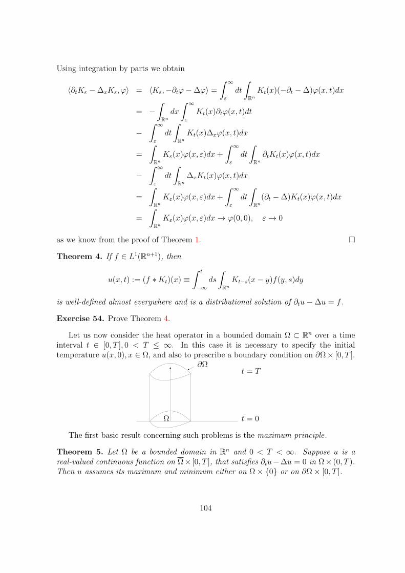
Using integration by parts we obtain
〈∂tKε −∆xKε, ϕ〉 = 〈Kε,−∂tϕ−∆ϕ〉 =∫ ∞
ε
dt
∫
Rn
Kt(x)(−∂t −∆)ϕ(x, t)dx
= −∫
Rn
dx
∫ ∞
ε
Kt(x)∂tϕ(x, t)dt
−∫ ∞
ε
dt
∫
Rn
Kt(x)∆xϕ(x, t)dx
=
∫
Rn
Kε(x)ϕ(x, ε)dx+
∫ ∞
ε
dt
∫
Rn
∂tKt(x)ϕ(x, t)dx
−∫ ∞
ε
dt
∫
Rn
∆xKt(x)ϕ(x, t)dx
=
∫
Rn
Kε(x)ϕ(x, ε)dx+
∫ ∞
ε
dt
∫
Rn
(∂t −∆)Kt(x)ϕ(x, t)dx
=
∫
Rn
Kε(x)ϕ(x, ε)dx→ ϕ(0, 0), ε→ 0
as we know from the proof of Theorem 1.
Theorem 4. If f ∈ L1(Rn+1), then
u(x, t) := (f ∗Kt)(x) ≡∫ t
−∞ds
∫
Rn
Kt−s(x− y)f(y, s)dy
is well-defined almost everywhere and is a distributional solution of ∂tu−∆u = f .
Exercise 54. Prove Theorem 4.
Let us now consider the heat operator in a bounded domain Ω ⊂ Rn over a timeinterval t ∈ [0, T ], 0 < T ≤ ∞. In this case it is necessary to specify the initialtemperature u(x, 0), x ∈ Ω, and also to prescribe a boundary condition on ∂Ω× [0, T ].
t = T
t = 0Ω
∂Ω
The first basic result concerning such problems is the maximum principle.
Theorem 5. Let Ω be a bounded domain in Rn and 0 < T < ∞. Suppose u is areal-valued continuous function on Ω× [0, T ], that satisfies ∂tu−∆u = 0 in Ω× (0, T ).Then u assumes its maximum and minimum either on Ω× 0 or on ∂Ω× [0, T ].
104

Proof. Given ε > 0, set v(x, t) := u(x, t)+ ε|x|2. Then ∂tv−∆v = −2nε. Suppose 0 <T ′ < T . If maximum of v in Ω× [0, T ′] occurs at an interior point of Ω×(0, T ′) then thefirst derivatives ∇x,tv vanish there and the second derivative ∂2j v for any j = 1, 2, . . . , nis nonpositive (consider v(x, t) as a function of one variable xj, j = 1, 2, . . . , n). Inparticular, ∂tv = 0 and ∆v ≤ 0, which contradicts with ∂tv − ∆v = −2nε < 0 and∆v = 2nε > 0.
Likewise, if the maximum occurs in Ω×T ′, then ∂tv(x, T ′) ≥ 0 and ∆v(x, T ′) ≤ 0which contradicts with ∂tv −∆v < 0. Therefore,
maxΩ×[0,T ′]
u ≤ maxΩ×[0,T ′]
v ≤ max(Ω×0)∪(∂Ω×[0,T ′])
u+ εmaxΩ
|x|2.
It follows that for ε→ 0 and T ′ → T ,
maxΩ×[0,T ]
u ≤ max(Ω×0)∪(∂Ω×[0,T ])
u.
Replacing u by −u we can obtain the same result for the minimum.
Corollary (Uniqueness). There is at most one continuous function u(x, t) in Ω ×[0, T ], 0 < T <∞, which agrees with a given continuous function f(x) in Ω×0, withg(x, t) on ∂Ω× [0, T ] and satisfies ∂tu−∆u = 0.
Let us look now more closely at the following problem:
∂tu−∆u = 0, in Ω× (0,∞)
u(x, 0) = f(x), in Ω
u(x, t) = 0, on ∂Ω× (0,∞).
(9.4)
This problem can be solved by the method of separation of variables. We begin bylooking for solution of the form
u(x, t) = F (x)G(t).
Then∂tu−∆u = FG′ −G∆xF = 0
if and only ifG′
G=
∆F
F:= −λ2
orG′ + λ2G = 0, ∆F + λ2F = 0,
for some constant λ. The first equation has the general solution
G(t) = ce−λ2t,
105

where c is an arbitrary constant. Without loss of generality we assume that c = 1. Itfollows from (9.4) that
∆F = −λ2F, in Ω
F = 0, on ∂Ω,(9.5)
because u(x, t) = F (x)G(t) and G(0) = 1.It remains to solve (9.5) which is an eigenvalue (spectral) problem for the Laplacian
with Dirichlet boundary condition. It is known that the problem (9.5) has infinitelymany solutions Fj(x)∞j=1 with corresponding
λ2j∞j=1
. The numbers −λ2j are called
eigenvalues and Fj(x) are called eigenfunctions of the Laplacian. It is also known thatλj > 0, j = 1, 2, . . ., λ2j → ∞ and Fj(x)∞j=1 can be chosen as complete orthonormal
set in L2(Ω) (or Fj(x)∞j=1 forms an orthonormal basis of L2(Ω)). This fact allows usto represent f(x) in terms of Fourier series
f(x) =∞∑
j=1
fjFj(x), (9.6)
where fj = (f, Fj)L2(Ω) are called the Fourier coefficients of f with respect to Fj∞j=1.If we take now
u(x, t) =∞∑
j=1
fjFj(x)e−λ2j t, (9.7)
then we may conclude (at least formally) that
∂tu = −∞∑
j=1
fjλ2jFj(x)e
−λ2j t =∞∑
j=1
fj∆Fj(x)e−λ2j t = ∆u,
that is, u(x, t) from (9.7) satisfies the heat equation and u(x, t) = 0 on ∂Ω× (0,∞). Itremains to prove that u(x, t) satisfies the initial condition and to determine for whichfunctions f(x) the series (9.6) converges and in what sense. This is the main questionin the Fourier method.
It is clear that the series (9.6) and (9.7) (for t ≥ 0) converge in the sense ofL2(Ω). It is also clear that if f ∈ C1(Ω) vanishes at the boundary then u will vanishon ∂Ω × (0,∞) and one easily verifies that u is a distributional solution of the heatequation (t > 0). Hence it is a classical solution since u(x, t) ∈ C∞(Ω × (0,∞)) (seeCorollary 2 of Theorem 1).
Similar considerations apply to the problem
∂tu−∆u = 0, in Ω× (0,∞)
u(x, 0) = f(x), in Ω
∂νu(x, t) = 0, on ∂Ω× (0,∞).
This problem boils down to finding orthonormal basis of eigenfunctions for Laplacianwith the Neumann boundary condition. Let us remark that for this problem, 0 isalways an eigenvalue and 1 is an eigenfunction.
106

Exercise 55. Prove that u(x, t) of the form (9.7) is a distributional solution of theheat equation in Ω× (0,∞).
Exercise 56. Show that∫ π0|u(x, t)|2dx is a decreasing function of t > 0, where u(x, t)
is the solution of ut − uxx = 0, 0 < x < π, t > 0
u(0, t) = u(π, t) = 0, t > 0.
107
10 The Wave Operator
The wave equation is defined as
∂2t u(x, t)−∆xu(x, t) = 0, (x, t) ∈ Rn × R. (10.1)
The wave equation is satisfied exactly by the components of the classical electromag-netic field in vacuum.
The characteristic variety of (10.1) is
charx(L) =(ξ, τ) ∈ Rn+1 : (ξ, τ) 6= 0, τ 2 = |ξ|2
and it is called the light cone. Accordingly, we call
(ξ, τ) ∈ charx(L) : τ > 0
and(ξ, τ) ∈ charx(L) : τ < 0
the forward and backward light cone, respectively.The wave operator is a prototype of hyperbolic operators. It means that the main
symbol ∑
|α|+j=kaα(x, t)ξ
ατ j
has k distinct real roots with respect to τ .
Theorem 1. Suppose u(x, t) is C2 function and that ∂2t u−∆u = 0. Suppose also thatu = 0 and ∂νu = 0 on the ball B = (x, 0) : |x− x0| ≤ t0 in the hyperplane t = 0.Then u = 0 in the region Ω = (x, t) : 0 ≤ t ≤ t0, |x− x0| ≤ t0 − t.
Proof. By considering real and imaginary parts we may assume that u is real. Denoteby Bt = x : |x− x0| ≤ t0 − t. Let us consider the following integral
E(t) =1
2
∫
Bt
((ut)
2 + |∇xu|2)dx
which represents the energy of the wave in Bt at time t. Next,
E ′(t) =
∫
Bt
(ututt +
n∑
j=1
∂ju(∂ju)t
)dx
− 1
2
∫
∂Bt
((ut)
2 + |∇xu|2)dσ(x) := I1 + I2.
108
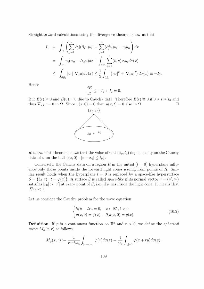
Straightforward calculations using the divergence theorem show us that
I1 =
∫
Bt
(n∑
j=1
∂j[(∂ju)ut]−n∑
j=1
(∂2ju)ut + ututt
)dx
=
∫
Bt
ut(utt −∆xu)dx+
∫
∂Bt
n∑
j=1
(∂ju)νjutdσ(x)
≤∫
∂Bt
|ut| |∇xu|dσ(x) ≤1
2
∫
∂Bt
(|ut|2 + |∇xu|2
)dσ(x) ≡ −I2.
HencedE
dt≤ −I2 + I2 = 0.
But E(t) ≥ 0 and E(0) = 0 due to Cauchy data. Therefore E(t) ≡ 0 if 0 ≤ t ≤ t0 andthus ∇x,tu = 0 in Ω. Since u(x, 0) = 0 then u(x, t) = 0 also in Ω.
b
b
x0t0
(x0, t0)
Remark. This theorem shows that the value of u at (x0, t0) depends only on the Cauchydata of u on the ball (x, 0) : |x− x0| ≤ t0.
Conversely, the Cauchy data on a region R in the initial (t = 0) hyperplane influ-ence only those points inside the forward light cones issuing from points of R. Sim-ilar result holds when the hyperplane t = 0 is replaced by a space-like hypersurfaceS = (x, t) : t = ϕ(x). A surface S is called space-like if its normal vector ν = (ν ′, ν0)satisfies |ν0| > |ν ′| at every point of S, i.e., if ν lies inside the light cone. It means that|∇ϕ| < 1.
Let us consider the Cauchy problem for the wave equation:
∂2t u−∆u = 0, x ∈ Rn, t > 0
u(x, 0) = f(x), ∂tu(x, 0) = g(x).(10.2)
Definition. If ϕ is a continuous function on Rn and r > 0, we define the sphericalmean Mϕ(x, r) as follows:
Mϕ(x, r) :=1
rn−1ωn
∫
|x−z|=rϕ(z)dσ(z) =
1
ωn
∫
|y|=1
ϕ(x+ ry)dσ(y).
109

Lemma 1. If ϕ is a C2 function on Rn, then Mϕ(x, 0) = ϕ(x) and
∆xMϕ(x, r) =
(∂2r +
n− 1
r∂r
)Mϕ(x, r).
Proof. It is clear that
Mϕ(x, 0) =1
ωn
∫
|y|=1
ϕ(x)dσ(y) = ϕ(x).
For the second part we have, by the divergence theorem, that
∂rMϕ(x, r) =1
ωn
∫
|y|=1
n∑
j=1
yj∂jϕ(x+ ry)dσ(y) =1
ωn
∫
|y|≤1
r∆ϕ(x+ ry)dy
=1
rn−1ωn
∫
|z|≤r∆ϕ(x+ z)dz
=1
rn−1ωn
∫ r
0
ρn−1dρ
∫
|y|=1
∆ϕ(x+ ρy)dσ(y).
That’s why we have
∂r(rn−1∂rMϕ(x, r)
)=rn−1
ωn
∫
|y|=1
∆ϕ(x+ ry)dσ(y) ≡ rn−1∆xMϕ(x, r).
It implies that
(n− 1)rn−2∂rMϕ(x, r) + rn−1∂2rMϕ(x, r) = rn−1∆xMϕ(x, r)
and proves the claim.
Corollary. Suppose u(x, t) is a C2 function on Rn+1 and let
Mu(x, r, t) =1
rn−1ωn
∫
|x−z|=ru(z, t)dσ(z) =
1
ωn
∫
|y|=1
u(x+ ry, t)dσ(y).
Then u(x, t) satisfies the wave equation if and only if
(∂2r +
n− 1
r∂r
)Mu(x, r, t) = ∂2tMu(x, r, t). (10.3)
Lemma 2. If ϕ ∈ Ck+1(R), k ≥ 1, then
∂2r
(1
r∂r
)k−1 (r2k−1ϕ(r)
)=
(∂rr
)k(r2kϕ′).
110
Proof. We employ induction with respect to k. If k = 1 then
∂2r
(1
r∂r
)k−1 (r2k−1ϕ(r)
)= ∂2r (rϕ) = ∂r(ϕ+ rϕ′) = 2ϕ′ + rϕ′′
and (∂rr
)k(r2kϕ′) =
(∂rr
)(r2ϕ′) = 2ϕ′ + rϕ′′.
Assume that
∂2r
(1
r∂r
)k−1 (r2k−1ϕ(r)
)=
(∂rr
)k(r2kϕ′).
Then
∂2r
(1
r∂r
)k (r2k+1ϕ(r)
)= ∂2r
(1
r∂r
)k−1(∂rr
(r2k+1ϕ
))
= ∂2r
(1
r∂r
)k−1 ((2k + 1)r2k−1ϕ+ r2kϕ′)
= (2k + 1)∂2r
(1
r∂r
)k−1 (r2k−1ϕ
)+ ∂2r
(1
r∂r
)k−1 (r2kϕ′)
= (2k + 1)
(∂rr
)k (r2kϕ′)+
(∂rr
)k(r2k(rϕ′)′)
=
(∂rr
)k ((2k + 1)r2kϕ′ + r2k(rϕ′)′
)
=
(∂rr
)k ((2k + 1)r2kϕ′ + r2kϕ′ + r2k+1ϕ′′)
=
(∂rr
)k ((2k + 2)r2kϕ′ + r2k+1ϕ′′)
=
(∂rr
)k+1 (r2k+2ϕ′) .
Corollary of Lemma 1 gives that if u(x, t) is a solution of the wave equation (10.1)in Rn × R then Mu(x, r, t) satisfies (10.3), i.e.,
(∂2r +
n− 1
r∂r
)Mu = ∂2tMu,
with initial conditions:
Mu(x, r, 0) =Mf (x, r), ∂tMu(x, r, 0) =Mg(x, r), (10.4)
since u(x, 0) = f(x) and ∂tu(x, 0) = g(x).
111

Let us set
u(x, r, t) :=
(∂rr
)n−32 (
rn−2Mu
)≡ TMu,
f(x, r) := TMf , g(x, r) := TMg
(10.5)
for n = 2k + 1, k = 1, 2, . . ..
Lemma 3. The following is true:
∂2r u = ∂2t u
u|t=0 = f , ∂tu|t=0 = g,(10.6)
where u, f and g are defined in (10.5).
Proof. Since n = 2k + 1 then n−32
= k − 1 and n− 2 = 2k − 1. Hence we obtain fromLemmata 1 and 2 that
∂2r u = ∂2rTMu = ∂2r
(∂rr
)k−1 (r2k−1Mu
)=
(∂rr
)k (r2k∂rMu
)
=
(∂rr
)k−1 (2kr2k−2∂rMu + r2k−1∂2rMu
)
=
(∂rr
)k−1(r2k−1
(∂2rMu +
n− 1
r∂rMu
))=
(∂rr
)k−1 (r2k−1∂2tMu
)
= ∂2t
(∂rr
)k−1 (r2k−1Mu
)= ∂2t u.
Moreover, the initial conditions are satisfied due to (10.4) and (10.5).
But now, since (10.6) is a one-dimensional problem, we may conclude that u(x, r, t)from Lemma 3 is equal to
u(x, r, t) =1
2
f(x, r + t) + f(x, r − t) +
∫ r+t
r−tg(x, s)ds
. (10.7)
Lemma 4. If n = 2k + 1, k = 1, 2, . . ., then
Mu(x, 0, t) = limr→0
u(x, r, t)
(n− 2)!!r,
where (n − 2)!! = 1 · 3 · 5 · · · (n − 2), is the solution of (10.2). We have even more,namely,
u(x, t) =1
(n− 2)!!
(∂rf |r=t + g(x, t)
). (10.8)
112
Proof. By (10.5) we have
u(x, r, t) =
(∂rr
)k−1 (r2k−1Mu
)=
(∂rr
)k−2 ((2k − 1)r2k−3Mu + r2k−2∂rMu
)
= (2k − 1)(2k − 3) · · · 1 ·Mur +O(r2)
oru(x, r, t)
(n− 2)!!r=Mu +O(r).
Hence
Mu(x, 0, t) = limr→0
u(x, r, t)
(n− 2)!!r.
But by definition of Mu we have that Mu(x, 0, t) = u(x, t), where u(x, t) is the solutionof (10.2). The initial conditions in (10.2) are satisfied due to (10.5). Next, sinceu(x, r, t) satisfies (10.7) then
limr→0
u(x, r, t)
(n− 2)!!r=
1
2(n− 2)!!
(limr→0
f(x, r + t) + f(x, r − t)
r+ lim
r→0
1
r
∫ r+t
r−tg(x, s)ds
)
=1
2(n− 2)!!
(∂rf |r=t + ∂rf |r=−t + g(x, t)− g(x,−t)
),
because f(x, t) and g(x, t) are odd functions of t. That’s why we finally obtain
limr→0
u(x, r, t)
(n− 2)!!r=
1
(n− 2)!!
(∂rf |r=t + g(x, t)
).
Now we are in the position to prove the main theorem for odd n ≥ 3.
Theorem 2. Suppose that n = 2k+1, k = 1, 2, . . .. If f ∈ Cn+32 (Rn) and g ∈ C
n+12 (Rn)
then
u(x, t) =1
(n− 2)!!ωn
∂t
(∂tt
)n−32(tn−2
∫
|y|=1
f(x+ ty)dσ(y)
)
+
(∂tt
)n−32(tn−2
∫
|y|=1
g(x+ ty)dσ(y)
) (10.9)
solves (10.2).
Proof. Due to Lemmata 3 and 4 u(x, t) given by (10.8) is the solution of the waveequation. It remains only to check that this u satisfies the initial conditions. But(10.9) gives us for small t that
u(x, t) =Mf (x, t) + tMg(x, t) +O(t2).
113

It implies that
u(x, 0) =Mf (x, 0) = f(x), ∂tu(x, 0) = ∂tMf (x, 0) +Mg(x, 0) = g(x).
The last equality follows from the fact that Mf (x, t) is even in t and so its derivativevanishes at t = 0.
Remark. If n = 3 then (10.9) becomes
u(x, t) =1
4π
∂t
(t
∫
|y|=1
f(x+ ty)dσ(y)
)+ t
∫
|y|=1
g(x+ ty)dσ(y)
≡ 1
4π
∫
|y|=1
f(x+ ty)dσ(y) + t
∫
|y|=1
∇f(x+ ty) · ydσ(y)
+ t
∫
|y|=1
g(x+ ty)dσ(y)
.
The solution of (10.2) for even n is readily derived from the solution for odd n by”the method of descent”. This is just the trivial observation: if u is a solution of thewave equation in Rn+1 × R that does not depend on xn+1 then u satisfies the waveequation in Rn × R. Thus to solve (10.2) in Rn × R with even n, we think of f and gas functions on Rn+1 which are independent of xn+1.
Theorem 3. Suppose that n is even. If f ∈ Cn+42 (Rn) and g ∈ C
n+22 (Rn) then the
function
u(x, t) =2
(n− 1)!!ωn+1
∂t
(∂tt
)n−22
(tn−1
∫
|y|≤1
f(x+ ty)√1− y2
dy
)
+
(∂tt
)n−22
(tn−1
∫
|y|≤1
g(x+ ty)√1− y2
dy
) (10.10)
solves the Cauchy problem (10.2).
Proof. If n is even then n + 1 is odd and n + 1 ≥ 3. That’s why we can apply (10.9)in Rn+1 × R to get that
u(x, t) =1
(n− 1)!!ωn+1
∂t
(∂tt
)n−22
(tn−1
∫
y21+···+y2n+y2n+1=1
f(x+ ty + tyn+1)dσ(y)
)
+
(∂tt
)n−22
(tn−1
∫
y21+···+y2n+y2n+1=1
g(x+ ty + tyn+1)dσ(y)
),
(10.11)
where y = (y, yn+1), solves (10.2) in Rn+1 × R (formally). But if we assume nowthat f and g do not depend on xn+1 then u(x, t) does not depend on xn+1 either and
114

solves (10.2) in Rn×R. It remains only to calculate the integrals in (10.11) under thisassumption. We have
∫
|y|2+y2n+1=1
f(x+ ty + tyn+1)dσ(y) =
∫
|y|2+y2n+1=1
f(x+ ty)dσ(y)
= 2
∫
|y|≤1
f(x+ ty)dy√
1− |y|2,
because we have the upper and lower hemispheres of the sphere |y|2 + y2n+1 = 1.Similarly for the second integral in (10.11). This proves the theorem.
Remark. If n = 2 then (10.10) becomes
u(x, t) =1
2π
∂t
(t
∫
|y|≤1
f(x+ ty)√1− y2
dy
)+ t
∫
|y|≤1
g(x+ ty)√1− y2
dy
.
Now we consider the Cauchy problem for the inhomogeneous wave equation
∂2t u−∆xu = w(x, t)
u(x, 0) = f(x), ∂tu(x, 0) = g(x).(10.12)
We look for the solution u(x, t) of (10.12) as u = u1 + u2, where
∂2t u1 −∆u1 = 0
u1(x, 0) = f(x), ∂tu1(x, 0) = g(x),(A)
and ∂2t u2 −∆u2 = w
u2(x, 0) = ∂tu2(x, 0) = 0.(B)
For the problem (B) we will use a method known as Duhamel’s principle.
Theorem 4. Suppose w ∈ C[n2 ]+1(Rn × R). For s ∈ R let v(x, t; s) be the solution of
∂2t v(x, t; s)−∆xv(x, t; s) = 0
v(x, 0; s) = 0, ∂tv(x, 0; s) = w(x, s).
Then
u(x, t) :=
∫ t
0
v(x, t− s; s)ds
solves (B).
115

Proof. By definition of u(x, t) it is clear that u(x, 0) = 0. We also have
∂tu(x, t) = v(x, 0; t) +
∫ t
0
∂tv(x, t− s; s)ds.
It implies that ∂tu(x, 0) = v(x, 0; 0) = 0. Differentiating once more in t we can see that
∂2t u(x, t) = ∂t(v(x, 0; t)) + ∂tv(x, 0; t) +
∫ t
0
∂2t v(x, t− s; s)ds
= w(x, t) +
∫ t
0
∆xv(x, t− s; s)ds
= w(x, t) + ∆x
∫ t
0
v(x, t− s; s)ds = w(x, t) + ∆xu.
Thus u solves (B) and the theorem is proved.
Let us consider again the homogeneous Cauchy problem (10.2). Applying theFourier transform with respect to x gives
∂2t u(ξ, t) + |ξ|2u(ξ, t) = 0
u(ξ, 0) = f(ξ), ∂tu(ξ, 0) = g(ξ).
But this ordinary differential equation with initial conditions can be easily solved toobtain
u(ξ, t) = f(ξ) cos(|ξ|t) + g(ξ)sin(|ξ|t)
|ξ| ≡ f(ξ)∂t
(sin(|ξ|t)
|ξ|
)+ g(ξ)
sin(|ξ|t)|ξ| .
It implies that
u(x, t) = F−1
(f(ξ)∂t
sin(|ξ|t)|ξ|
)+ F−1
(g(ξ)
sin(|ξ|t)|ξ|
)
= f ∗ ∂t((2π)−n/2F−1
(sin(|ξ|t)
|ξ|
))+ g ∗
((2π)−n/2F−1
(sin(|ξ|t)
|ξ|
))
= f ∗ ∂tΦ(x, t) + g ∗ Φ(x, t), (10.13)
where Φ(x, t) = (2π)−n/2F−1(
sin(|ξ|t)|ξ|
).
The next step is to try to solve the equation
∂2t F (x, t)−∆xF (x, t) = δ(x)δ(t).
By Fourier transform in x we obtain
∂2t F (ξ, t) + |ξ|2F (ξ, t) = (2π)−n/2δ(t).
116

That’s why F must be a solution of ∂2t u+ |ξ|2u = 0 for t 6= 0. Therefore
F (ξ, t) =
a(ξ) cos(|ξ|t) + b(ξ) sin(|ξ|t), t < 0
c(ξ) cos(|ξ|t) + d(ξ) sin(|ξ|t), t > 0.
To obtain the delta function at t = 0 we require that F is continuous at t = 0 but ∂tFhas a jump of size (2π)−n/2 at t = 0. So we have
a(ξ) = c(ξ), |ξ|(d(ξ)− b(ξ)) = (2π)−n/2.
This gives two equations for the four unknown coefficients a, b, c and d. But it isreasonable to require F (x, t) ≡ 0 for t < 0. Hence, a = b = c = 0 and d = (2π)−n/2 1
|ξ| .That’s why
F (ξ, t) =
(2π)−n/2 sin(|ξ|t)|ξ| , t > 0
0, t < 0.(10.14)
If we compare (10.13) and (10.14) we may conclude that
F (x, t) = (2π)−n/2F−1ξ
(sin(|ξ|t)
|ξ|
), t > 0
and
Φ+(x, t) =
Φ(x, t), t > 0
0, t < 0
is the fundamental solution of the wave equation, i.e., F (x, t) with t > 0.There is one more observation. If we compare (10.9) and (10.10) with (10.13) then
we may conclude that these three formulae are the same. Hence, we may calculate theinverse Fourier transform of
(2π)−n/2sin(|ξ|t)
|ξ|in odd and even dimensions respectively with (10.9) and (10.10). Actually, the resultis presented in these two formulae.
When solving the wave equation in the region Ω × (0,∞), where Ω is a boundeddomain in Rn, it is necessary to specify not only Cauchy data on Ω×0 but also someconditions on ∂Ω×(0,∞) to tell the wave what to do when it hits the boundary. If theboundary conditions on ∂Ω× (0,∞) are independent of t, the method of separation ofvariables can be used.
Let us (for example) consider the following problem:
∂2t u−∆xu = 0, in Ω× (0,∞)
u(x, 0) = f(x), ∂tu(x, 0) = g(x), in Ω
u(x, t) = 0, on ∂Ω× (0,∞).
(10.15)
117

We can look for solution u in the form u(x, t) = F (x)G(t) and get
∆F (x) + λ2F (x) = 0, in Ω
F (x) = 0, on ∂Ω,(10.16)
andG′′(t) + λ2G(t) = 0, 0 < t <∞. (10.17)
The general solution of (10.17) is
G(t) = a cos(λt) + b sin(λt).
Since (10.16) has infinitely many solutions Fj∞j=1 with correspondingλ2j∞j=1
, λ2j →+∞ (λj > 0) and Fj∞j=1 can be chosen as an orthonormal basis in L2(Ω), the solutionu(x, t) of (10.15) is of the form
u(x, t) =∞∑
j=1
Fj(x) (aj cos(λjt) + bj sin(λjt)) . (10.18)
At the same time f(x) and g(x) have the L2(Ω) representations
f(x) =∞∑
j=1
fjFj(x), g(x) =∞∑
j=1
gjFj(x), (10.19)
where fj = (f, Fj)L2 and gj = (g, Fj)L2 . It follows from (10.15) and (10.18) that
u(x, 0) =∞∑
j=1
ajFj(x), ut(x, 0) =∞∑
j=1
λjbjFj(x). (10.20)
Since (10.19) must be satisfied also we obtain
aj = fj, bj =1
λjgj.
Therefore, the solution u(x, t) of (10.15) has the form
u(x, t) =∞∑
j=1
Fj(x)
(fj cos(λjt) +
1
λjgj sin(λjt)
).
It is clear that all series (10.18),(10.19) and (10.20) converge in L2(Ω), because Fj∞j=1
is an orthonormal basis in L2(Ω). It remains only to investigate the convergence ofthese series in stronger norms (which depends on f and g, or more precisely, on theirsmoothness).
The Neumann problem with ∂νu(x, t), x ∈ ∂Ω, can be considered in a similarmanner.
118
Index
δ-function, 8
a translation, 57approximation to the identity, 5
biharmonic equation, 11Burgers equation, 16
Cauchy data, 17Cauchy problem, 17Cauchy-Kowalevski theorem, 18Cauchy-Riemann operator, 11, 63characteristic, 11characteristic form, 11characteristic variety, 11continuous kernel, 84convolution, 4
d’Alembert formula, 48differential operator, 10Dirichlet problem, 51distribution, 8distributional solution, 10divergence theorem, 4double layer potential, 84Duhamel’s principle, 115
eigenvalue problem, 33eikonal equation, 10elliptic differential operator, 11even function, 23evolution equation, 10exterior Dirichlet problem, 82exterior Neumann problem, 82
Fourier cosine series, 26Fourier inversion formula, 7Fourier series, 25Fourier sine series, 26Fourier transform, 6fundamental period, 23fundamental solution, 63
Gaussian kernel, 100Gibbs phenomenon, 29gradient, 10Green’s function, 71Green’s identities, 59
Hans Lewy example, 21harmonic function, 59Harnack’s inequality, 80heat equation, 10, 32heat operator, 100hyperplane, 3hypersurface, 3
ill-posed problem, 21integral curves, 12interior Dirichlet problem, 82interior Neumann problem, 82
Korteweg-de Vries equation, 11
Laplace equation, 51Laplace operator, 10, 57Laplacian, 10, 57linear superposition principle, 35Liouville’s theorem, 62
maximum principle, 61, 104mean value theorem, 60method of characteristics, 13multi-index, 1mutually orthogonal functions, 23
Neumann problem, 51non-characteristic, 11normal, 3
odd function, 23orthogonal complement, 96orthogonal functions, 23
periodic function, 23piecewise continuous function, 23
119

Plancherel theorem, 7Poisson equation, 10Poisson integral, 74Poisson kernel, 74principal symbol, 11
quasi-linear equation, 14
Reflection Principle, 80regular distribution, 8removable singularity, 80Riemann-Lebesgue lemma, 6rotation, 57
Schwartz space, 7separation of variables, 33Sine-Gordon equation, 11single layer potential, 84spherical mean, 109support, 7
telegrapher’s equation, 11tempered distribution, 9tubular neighborhood, 93
wave equation, 10, 44, 108wave operator, 108weak solution, 10well-posed problem, 20
Young’s inequality for convolution, 4
120


