~ 1 ~

CSIRO‐Monash Superannuation Research Cluster

Project 4: Fund Style and Optimal Asset Allocation, More Effective Indexing, and Exposure to Alternative Assets Via Hedge Fund Replication, Working Paper

Is fundamental indexation able to time the market?

Evidence from the Dow Jones Industrial Average

Paul Lajbcygiera,b, Doris Chena, Michael Dempseya aFaculty of Business and Economics, Department of Accounting & Finance, Monash University. bFaculty of Business and Economics, Department of Econometrics and Business Statistics, Monash University.

28 November 2013

Preliminary Draft – Not for Public Distribution

Abstract

Fundamental Indexation (FI) creates a broad based market portfolio, like traditional market

capitalization weighted indices, but weights stock according to a firm’s economic size, not stock

price. In the context of the Dow Jones Industrial Average index, we find evidence of the ability of FI

to time the market in a single period of crisis, the technology boom and bust (August 1998 to August

2002). Against this, FI underperforms against a market capital–weighted index in the global financial

crisis, which undermines a good deal of FI’s claim to success. Overall, the superior outperformance of

FI is clearly linked to loadings on the Fama and French book-to-market and size factors. We find that

equal-weighted indexation, which represents a traditional form of non-market capitalization, performs

well and appears to be successful (ignoring transaction costs) at timing the market.

ACKNOWLEDGEMENTS: THIS RESEARCH WAS SUPPORTED BY THE CSIRO-MONASH SUPERANNUATION

RESEARCH CLUSTER, A COLLABORATION BETWEEN CSIRO, MONASH UNIVERSITY, GRIFFITH UNIVERSITY, THE UNIVERSITY OF WESTERN AUSTRALIA, THE UNIVERSITY OF WARWICK, AND STAKEHOLDERS OF THE

RETIREMENT SYSTEM IN THE INTEREST OF BETTER OUTCOMES FOR ALL .

THIS RESEARCH WAS ALSO SUPPORTED BY AN AUSTRALIA RESEARCH COUNCIL LINKAGE GRANT.

~ 2 ~

Is fundamental indexation able to time the market?

Evidence from the Dow Jones Industrial Average

Abstract

Fundamental Indexation (FI) creates a broad based market portfolio, like traditional market

capitalization weighted indices, but weights stock according to a firm’s economic size, not stock

price. Consistent with the theoretical underpinnings of fundamental indexation (FI) as a strategy that

seeks to avoid the collapse of “bubbles” due to stock price noise, we investigate whether FI portfolios

are capable of market timing. In the context of the Dow Jones Industrial Average index, we find

evidence of the ability of FI to time the market in a single period of crisis, the technology boom and

bust (August 1998 to August 2002). Against this, FI underperforms against a market capital–weighted

index in the global financial crisis, which undermines a good deal of FI’s claim to success. Overall,

the superior outperformance of FI is clearly linked to loadings on the Fama and French book-to-

market and size factors. Ironically, we find that equal-weighted indexation, which represents a

traditional form of non-market capitalization, performs well and appears to be successful (ignoring

transaction costs) at timing the market.

~ 3 ~

1. Introduction

It can be argued that market capitalization-weighted indexes (MCWIs) are suboptimal since, by

construction, they must overweight overvalued shares and underweight undervalued shares (Treynor,

2005). To counter this tendency, Arnott et al. (2005c) identify a form of indexing, which they call

fundamental indexation (FI), where the weights are assigned to stocks on the basis of non-market

measures of a firm’s size: book value, revenue, cash flow, dividend, sales, and even employee

numbers.1 Their claim is that such a preferred weighting approach allows assets to be proportioned to

reflect more accurately the true “economic” weightings of portfolio firms, and that FI is thereby

immune to pricing “bubbles.”

A number of authors confirm that FI outperforms when benchmarked against the traditional

capital asset pricing model (CAPM), but does not outperform against the Fama–French (1993, 1996)

three-factor model, which has additional risk premiums for high book-to-equity and small-firm stocks

(e.g., Jun and Malkiel (2007), Blitz and Swinkels (2008), McQuarrie (2008), Malkiel and Jun (2009)).

Since FI indexes, by construction, display a bias toward higher book-to-market equity and small-firm

stocks, it is possible to interpret FI’s reported performances as a repackaging of known “value” (high

book-to-market equity) and “small firm size” effects.

This paper seeks to determine whether the outperformance of FI can be separated from that of

exposure to the Fama–French factors. Following the theoretical underpinnings of FI as a strategy of

avoiding bubbles in individual prices, FI should benefit from those periods when market bubbles are

corrected, as well as from individual stock price corrections. Thus, we investigate whether FI is

capable of timing the market at the level of both ongoing market fluctuations and major market

crises.2

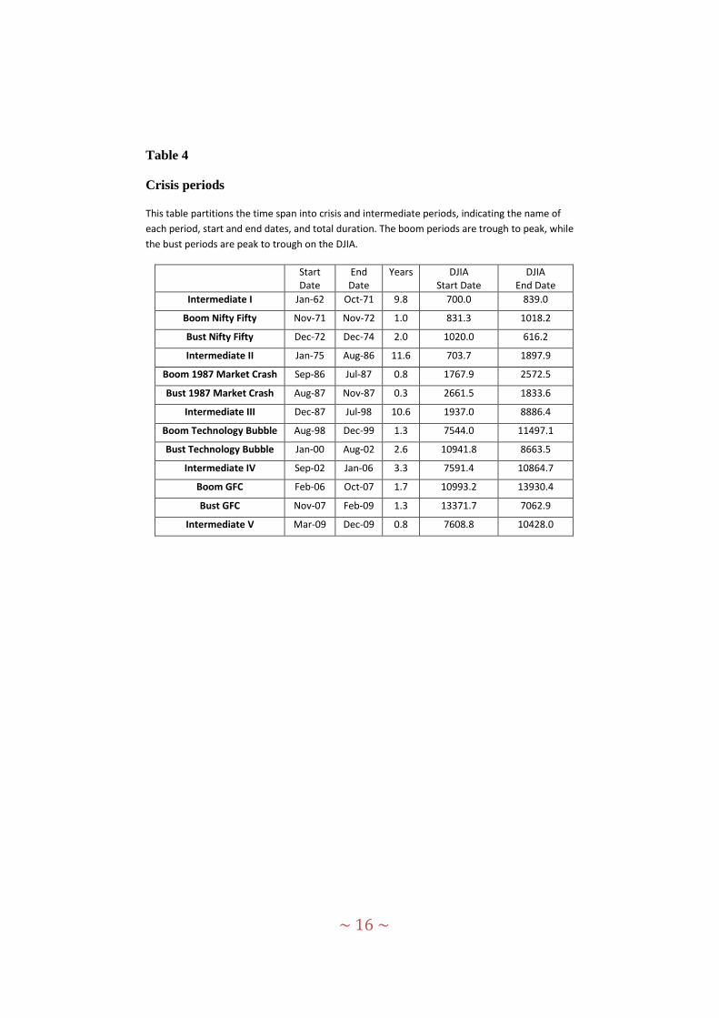
For this purpose, we obtain the stocks of the Dow Jones Industrial Average index (DJIA),

which provide 48 years of reliable stock market data over cycles that include the Nifty Fifty era of the

1970s, the 1987 stock market crash, the tech boom and bust of 2000, and the recent global financial

crisis of 2008. The DJIA stocks have high liquidity, volume, and depth, and consequently low noise

and high market efficiency compared with stocks of smaller firms. These features imply a challenging

environment for FI, since the “noise” effect that FI seeks to manipulate is suppressed in these stocks.

Our main findings are as follows. Over the period 1962–2009, we find evidence that the

stocks of the DJIA formed as fundamental indexes provide superior returns relative to a price-

weighted index (PWI). However, we find no evidence that the FI outperformance can be differentially

attributed between up- and down-market movements in any consistent manner. We do, however, find

1 In their study, the authors find that their FI realizes higher returns (excess returns of 1.97% per annum) with

similar or lower volatility than benchmark capitalization-weighted indexes such as the Standard & Poor's 500

and Russell 1000. Consequently, they suggest that fundamental indexes provide the basis for implementing

passive investment strategies that maintain the characteristics of index investing but avoid the noise due to

market prices. 2 In an on-line debate, Arnott suggested that although FI’s outperformance relies on exposure to the Fama–

French factors, an additional source of FI’s success is in its ability to time the market, tilting toward value at

appropriate times in the market cycle, which provides approximately 30% of FI’s success (see Arnott and

Sauter(2009)).

~ 4 ~

evidence that the success of FI can in part be attributed to its ability to time the market in one

particular period, namely, the technology bust of the early 2000s (January 2000 to August 2002),

when FI was able to value-tilt away from the excesses of this period prior to the collapse of

technology stocks. Against this, FI underperforms markedly during the global financial crisis. Thus,

the global financial crisis undermines a good deal of FI’s claim to success3. Additionally, we find that

the outperformance of FI is largely accounted for in terms of the Fama–French three-factor model.

The rest of the paper is organized as follows. Section 2 presents the data and methodology.

Section 3 presents the results. Finally, Section 4 summarizes the paper’s conclusions.

2. Data and Methodology

(a) Data

Monthly data for the stocks of the DJIA for 1962–2009 are obtained from the Dow Jones official

website.4 Company annual fundamental data are collected from the Compustat database. Fundamental

data include the book value of equity,5 earnings before interest and tax (EBIT), depreciation (DP),

total dividends (DVT), and net income (NI). The monthly compounded holding period return which

includes dividends (RET) data are from the Center for Research in Security Prices (CRSP) database6

and are linked to the corresponding Compustat data through PERMNO (available from the merged

lists from CRSP/Compustat). The monthly Fama–French three-factor model–related data––market

portfolio return (RM), high-minus-low (HML), and small-minus-big (SMB) factors, as well as the risk-

free rates (Rf)––were downloaded from Kenneth French’s data library.7

(b) Methodology

FI can outperform standard indexing for three possible reasons: (i) better stock selection, (ii) better

stock weighting, and (iii) market timing. Different stock selections allow a FI portfolio to contain

different stocks than the index portfolio with which it is being compared (e.g., the stocks contained in

3 This is consistent with results reported in the financial press, which reported that the FTSE RAFI (Research

Affiliates Fundamental Index) US 1000 underperformed the S&P500 by almost 4% during this period (see

Greer (2011)),

4 The official website is: http://www.djindexes.com/mdsidx/downloads/DJIA_Hist_Comp.pdf. We use the data

to replicate the Dow Jones between 1962 and 2009. The generated DJIA is then reconciled with published

figures. About a dozen or so months had errors above 5 index points.

5 We calculate book value as the book value of stockholder equity (SEQ) plus balance sheet deferred taxes

(TXDITC) plus investment tax credits (ITCB) minus the redemption value of preferred stocks (PSTKRV). For the

sake of consistency, this is taken from Fama and French’s book equity calculation (thus, we do not use the book

value provided in CRSP/Compustat). The values are calculated in June of each year. Two versions of the Fama–

French book value formulas are implemented (differing on filtering conditions) and comparison data sets are

generated. The first is based on Fama and French (1993) and the second (as reported here) is based on personal

correspondence with Kenneth French. The differences are not material.

6 Monthly prices and number of shares outstanding are from the CRSP database. The CRSP output has a small

number of erroneous records, which are filtered out. These include missing year, duplicate records, and non-

unique PERMNOs.

7 See http://mba.tuck.dartmouth.edu/pages/faculty/ken.french/data_library.html.

~ 5 ~

the top 1,000 stocks using the FI criterion are not necessarily those of a capital-weighted counterpart,

as in the Russell 1,000). This study avoids differences due to different stock selections by constraining

FI to contain the same stocks as their market capitalization counterparts (similar to Branch and Cai

(2010); Hemminki and Puttonen (2008)). In this way, we focus on the differences in performance due

to either better stock weighting or market timing ability8.

We construct composite indexes using four fundamental variables: book value, cash flow,9

sales, and total dividends (as in Arnott et al., 2005a).10

To construct the FI composite index, we

average the weights based on the four fundamental variables (when the averages do not add to one,

we normalize the values across stocks). We also follow Arnott et al. (2005a), smoothing the

variability of the variables with five-year trailing averages for the fundamental variables other than

book value. The procedure requires that five years of historic data prior to a stock entering the index

be included. To allow for possible reporting delays between December and June, we lag the

construction of indexes to July of each year so that all annual reports are included (as per Fama and

French (1993)). The resulting July figures are then used monthly until the following June.

Four benchmark non–FI-based indexes are constructed: (1) the DJIA, which is a PWI,

adjusted for corporate actions (e.g., splits, mergers, replacements of companies in the index)11

, (2) a

PWI unadjusted with respect to the DJIA adjustment factor, (3) a DJIA MCWI, and (4) an equally

weighted index (EWI) of the stocks in the DJIA12

.

(i) FI indexes and the Fama–French three-factor model

We test FI performance against both the CAPM,

(1)

and the Fama–French (1993, 1996) three-factor model for the expected return on a stock’s equity, E(Rit):

(2)

8 Arnott et al (2005) argue that FI should include additional stock selected by their approach and not simply

reweight the stocks in an index as this leads to a portfolio that is concentrated in large, high book value stocks.

However, such a concentration may improve FI performance as Macquarrie (2008) shows that large high book

value stocks perform very well and are responsible for the outperformance of equally weighted indexation.

9 Depreciation added to earnings is used to compute cash flow (as in Desai et al., 2004).

10 As in Arnott et al. (2005), we exclude employment, because that information is not always available, and

revenue, due to its close correspondence with sales.

11 For details on the adjustment factor, refer to the Dow Jones document available at

http://www.cmegroup.com/trading/equity-index/files/djia-history-divisor.pdf.

12 McQuarrie (2008) p.38 asserts that a fix for “the problems inherent in pure cap-weighting can readily be

found in an equal-weight index. Performance relative to an equal-weight index represents the hurdle that RAFI

[i.e. FI] must surmount before its radical theoretical claims can be considered”.

~ 6 ~

where, [ ] , and are (a) the excess return on a broad market portfolio, (b) the difference

between the return on a portfolio of small-firm stocks and that on a portfolio of large-firm stocks (small minus big), and (c)

the difference between the return on a portfolio of high book-to-market stocks and that on a portfolio of low book-to-

market stocks (high minus low). The factor sensitivities, or loadings, , and are the slopes in the time series

regression,

( ) (3)

where the intercept measures the excess return, which is unexplained by the loading factors ,

.

(ii) FI and market timing

To identify the market timing ability of FI in outperforming market down periods, we use a 12-month

rolling window to estimate the value and size loadings of the FI composite index. To investigate

whether the loadings are effective in timing the market, we apply the Henriksson–Merton (1981)

model in the context of both the traditional CAPM,

( ) [ ( )] (4)

and the Fama–French three-factor model,

( ) [ ( )]

(5)

where are dummy variables equal to zero if the accompanied variable (excess

market return RMt - Rft, value premium , or size premium ) is positive, and -1

otherwise. Significant positive values for the coefficients ,

, and imply market timing

ability with regard to the corresponding risk premium.13

(iii) FI in crisis periods

We also apply the Fama–French and Henriksson–Merton (1981) models to examine the FI

performances during specific crisis and non-crisis periods separately between 1962 and 2009. The

boom periods are defined to be from the trough to the peak, while the bust periods are the subsequent

peak-to-trough periods on the DJIA.

3. Results

The overall outcomes for the benchmark indexes, the geometric and holding period returns, the

standard deviation (volatility) of the annual return of each of the indexes, and the Sharpe ratio are

13 Henriksson and Merton (1981) show that the errors are not independent and identically distributed but

increase as a function of the factor returns, and they suggest that corrections for heteroskedasticity are made,

although Henriksson (1984) provides conflicting evidence about their importance.

~ 7 ~

presented in Table 1. Table 1 reveals that all versions of the FI outperform the benchmark MCWI.14

However, the highest-performing index is the EWI15

suggesting, as McQuarrie (2008) state, that

“there is no need to resort to the elaborate procedures used to construct the RAFI” (p.37). Thus the

simplest form of non-MCWI is the most successful. The risk-adjusted Sharpe ratio ranks the dividend

and net income FIs highest, followed by the FI composite and the EWI.

[Table 1 about here]

Figure 1 plots the size and value “tilts” for the FI composite index (the difference between the

Fama-French size and value loadings for the FI composite and the corresponding loadings for the

MCWI index), estimated using a 48-month prior moving window of returns. The tilts are consistently

positive (although insignificant for size), implying that the FI composite is consistently tilted to stocks

of higher book value and smaller capitalization compared with a MCWI. Below the tilts, the shaded

curve represents the compounding accumulated outperformance of the FI composite index against the

MCWI at each point in time. The total outperformance of the FI composite over the MCWI is 47.8%,

compounded monthly over the entire period. Thus, the curve reveals those periods when the FI

composite was either outperforming the MCWI (increasing slope) or underperforming the MCWI

(decreasing slope). We observe that there are long periods when the relative performance of the FI

composite is correlated with the loadings on size and value.

[Figure 1 about here]

(a) FI indexes and the Fama–French three-factor model

The results of regressing the FI indexes on the Fama–French three-factor model as equation 3 are

displayed in Table 2. The coefficients , , and are significant at the 1% level (as expected, the

coefficients are negative due to the large capitalization of the DJIA stocks). However, the α values

for the indexes are insignificant from zero (with the exception of the DJIA, which has a negative

intercept α). Thus, consistent with prior studies, it is possible to attribute the outperformance of FI to

value and size risk exposures.

[Table 2 about here]

(b) FI and market timing

The findings for market timing using the Henriksson and Merton regressions for the FI portfolio

excess returns on the CAPM as equation 4 reveal no significant timing ability in outperforming

the down-market periods (available upon request). Thus, the ability of FI to outperform cap-

weighted indexes does not appear to be systematically related to a systematic avoidance of the

worst of down-market outcomes. The exception is for an EWI, which provides a statistically

significant positive coefficient. The regressions on the Fama–French three-factor model as

equation 5 tell a similar story, as summarized in Table 3. In addition, Table 3 confirms that the

14 Consistently, when we regress the FI indexes on the traditional CAPM as equation 1, we encounter positive α

values (not reported here).

15 The argument against an equal-weighting portfolio in practice is that (i) the costs of trading large volumes of

small capitalization stocks are prohibitive; and, (ii) the constant rebalancing required to achieve equal-weighting

leads to large turnover that erodes returns. This is less likely to be the case for the 30 large capitalization stocks

of the DJIA.

~ 8 ~

ability of FI to outperform cap-weighted indexes is not related to an ability to systematically

“time” weightings on either the market’s book to market value or size premiums as captured by

the Fama–French three-factor model. Again, the exception is for an EWI, which again provides

a statistically significant positive coefficient. For the DJIA, the is actually negative. A PWI

has a significantly negative weighting on the size factor, meaning that it significantly

overweights on small stocks in down markets, to its detriment.

[Table 3 about here]

(c) FI in crisis periods

We extend our search for market timing by examining various equity market ‘crisis’ periods over the

last 50 years. There are long periods (from February 1962 to mid-1971 and from March 1988 to

February 2000) when the FI index follows the market (i.e. MCWI) with similar perfromace. However,

there are three large increases that account for much of FI’s outperformance in periods of crisis: that

between mid-1972 and January 1977 (which incorporates the Nifty Fifty period), that between

January 1982 and March 1988 (which incorporates the boom and bust of the 1987 stock market crash),

and that between early 2000 and early 2007 (which incorporates the bursting of the technology bubble

and the period of the “great moderation”). However, the superior FI performance during the first two

of these periods does not appear to be particularly related to the crisis period. Thus, the FI indexes do

not significantly avoid the worst of the demise of the Nifty Fifty era or the worst of the October 1987

crash. There are also two periods that reveal substantial declines in FI performance in periods of crisis:

between October 1988 and December 1991 (encapsulating the recession of the early 1990s) and

between March 2007 and February 2009 (encapsulating the global banking crisis).

Table 4 summarizes the cycles of boom and bust,16

and Table 5 compares the MCWI and FI

composite performance in these periods17

. Outperformance (and underperformance) of FI appears to

occur at discrete points in history.18

FI outperforms both MCWI and EWI in the Nifty Fifty period by

approximately 3%; and in the Intermediate III period by about 9%. In particular, in the technology

bubble period FI outperforms EWI by 2% and MCWI by 9% (primarily due to very good performance

in the Bust period) and in the GFC period FI underperforms MCWI by 8% and EWI by 6%, primarily

due to the Bust GFC period.

[Insert Tables 4 and 5 about here]

16 Although these boom periods represent only a little over 10% of the time span, over 24% of the total (simple)

return for the FI composite is obtained during these times. In addition, whereas the bust periods represent almost

13% of the total time span, almost 32% of the total (simple) return losses for the FI composite were suffered

during these periods (see Figure 1 and Table 4).

17 Table 5 reports the compound returns earned in each period in order to facilitate comparisons between each

indexation method.

18 This observation appears consistent with Sauter’s statement that the bust of the Nifty Fifty and technology

stock bubbles greatly favored value stocks, and thereby FI (quoted in the Arnott–Sauter (2009) debate).

~ 9 ~

We also perform Fama–French and Henriksson–Merton regressions for the index

performances for the technology bubble period (August 1998 to August 2002) separately. The

positive α value over the market (i.e., CAPM) for the FIs are significant, but captured by the Fama–

French regressions. The implication is that the timing ability of FI is closely related to that of the

value factors in the Fama–French three-factor model.19

When this period is examined as separate

boom (August 1998 to December 1999) and bust (January 2000 to August 2002) periods, the

Henriksson–Merton regressions provide significant α values for both the EWI and the FI in the bust

period, although the coefficient is close to zero for EWI and significant for both only at 10%

significant levels. In addition, for the EWI, we find evidence of market timing on the value premium

(positive and significant coefficients). Thus, again, we have evidence that the effect of market

timing is most pronounced in the EWI (available upon request).

It is possible to identify the precise stocks that sustained the outperformance of the FI indexes

during both the technology bubble and the global financial crisis. First, if we compare FI composite

and MCWI portfolios at the beginning (Figure 2a) and the height of the technology bubble (Figure 2b),

we observe that FI portfolios successfully avoid overweighting tech stocks at the beginning of the

boom. FI overweighted AT&T by 2% and underweighted both IBM and HP (relative to a market

capital-weighted portfolio) by approximately 1%. This led to an underperformance by FI during this

period (Table 5). However, by the technology peak (December 1999), the FI composite was well

positioned for the bursting of the bubble. It was underweighted (relative to MCWI) technology stock:

Microsoft by about 12%, Intel by about 3.5%, and both Hewlett Packard and General Electric by

about 1% (it was approximately “at weight” for IBM and Honeywell). In addition, the FI composite

overweight Exxon Mobil by about 6% and General Motors by about 7%, companies in industries that

were non-technology related and immune to the bursting of the technology bubble. Although these

weightings together contributed to the 5% outperformance of the FI composite relative to a MCWI

(Table 5), most of the success was due to just two stocks: Microsoft stocks almost halved during the

year 2000, from $58.89 to $33.32 (December 11, 2000), and Intel did even worse, dropping over 70%,

from a high of $73.94 to $20.44 in the same year. The underweighting of these two stocks accounts

for over 90% of the outperformance of FI during this period.

[Insert Figure 2a and 2b about here]

Shortly before the global financial crisis (October 2007), FI had a significant overweight

position of 3.5% in both General Motors and CitiGroup, and a 1% overweight position in American

International Group, hereafter AIG (Figure 3a), whose positioning was responsible for the

underperformance of FI during the global financial crisis. At the nadir of the crisis (February 2009),

these overweight positions were amplified due to the price insensitivity of the FI composite (Figure

3b), with the overweight positions in GM increasing because of its near bankruptcy, AIG disappearing

from the DJIA list due to its government bailout, and Citigroup’s overweight position becoming 7%.

In addition, FI now had two new overweight positions: in General Electric (5%) and Bank of America

(3%). These overweight companies were also exposed to the risk factors that drove the financial

crisis. In fact, FI performed progressively worse as the crisis evolved.

19 In which case, the straightforward interpretation may be that each one explains the other. Although prior

papers give the three-factor model precedence, regulating FI to a manifestation of the Fama–French three-factor

model, the reverse interpretation may be equally valid, namely, that the value factor in the Fama–French model

is a manifestation of the noise phenomenon recognized by FI.

~ 10 ~

[Insert Figure 3a and 3b about here]

4. Discussion and Conclusion

In the context of the DJIA, we find evidence of the ability of FI to time the market in a single period

of crisis, which is the technology boom and bust (August 1998 to August 2002). Against this, FI

underperformed against an MCWI in the global financial crisis, which undermines a good deal of FI’s

claim to success. It appears, therefore, that the superior outperformance of FI remains inextricably

linked to loadings on the Fama–French book-to-market and size factors. An interesting question then

becomes whether the noise model of FI can be interpreted as a theoretical explanation for the

observed book-to-market effect. This possibility is advocated by the protagonists of FI (Arnott et al.

(2005a, 2005b), Arnott and Hsu (2008)). We see that this approach opens up exciting possibilities for

a theoretical underpinning of the Fama–French model in a framework of share price corrections.

Interestingly, we find that equal-weighted indexation, which represents a simple form of non-

market capitalization indexing, is highly successful (ignoring transaction costs). From a practical

perspective, the challenge for FI is to demonstrate that its strategy represents an optimal compromise

between the benefits of an equally weighted portfolio and those of following a market index.

~ 11 ~

References Arnott, R.D. and Hsu, J. (2008). “Noise, CAPM and the Size and Value Effects.” Journal of

Investment Management 6(1), 68–78.

Arnott, R.D., Hsu, J., Liu, J. and Markowitz, H. (2005a). “Does Noise Create the Size and

Value Effects?” SSRN paper, available at http://ssrn.com/abstract=936272.

Arnott, R.D., Hsu, J. and Markowitz, H. (2005b). “Does Noise Create the Fama–French Value and

Size Factors?” Research Affiliates Working Paper #WP275402.

Arnott, R.D., Hsu, J. and Moore, P. (2005c). “Fundamental Indexation.” Financial Analysts Journal

61(2), 83–99.

Arnott, R.D and Sauter, J. (2009). “Index Smack-down Debate”, http://podcast.financial-

planning.com/archive/the_index_smackdown.

Blitz, D. and Swinkels, L. (2008). “Fundamental Indexation: An Active Value Strategy in Disguise.”

Journal of Asset Management 9(4), 264–269.

Branch, B. and Cai, L. (2010). “Fundamental Weighting”, Journal of Applied Finance, 1, 64-77.

Desai, H., Rajgopal, S. and Venkatachalam, M. (2004). “Value-Glamour and Accrual Mispricing:

One Anomaly or Two?” Accounting Review 79(2), 355–385.

Fama, E. and French, K. (1993). “Common Risk Factors in the Returns on Stocks and Bonds.”

Journal of Financial Economics 33, 3–56.

Fama, E. and French, K. (1996). “Multifactor Explanations of Asset Pricing Anomalies.” Journal of

Finance 51, 55–84.

Greer, C. (2011). “Index Funds Get a Makeover”, Wall St Journal, 7/2/2011.

http://online.wsj.com/article/SB10001424052748703555804576101812395730494.html

Hemminki, J. and Puttonen, V. (2008), “Fundamental Indexation in Europe”, Journal of Asset

Management, 8, 401-405.

Henriksson, R.D. (1984). “Market Timing and Mutual Fund Performance: An Empirical

Investigation.” Journal of Business 57, 73–96.

Henriksson, R.D. and Merton, R.C. (1981). “On Market Timing and Investment Performance.”

Journal of Business 54, 513–533.

Jun, D. and Malkiel, B. (2007). “New Paradigms in Stock Market Indexing.” European Financial

Management 14(1), 118–126.

Malkiel, B. and Jun, D. (2009). “Creating Indexed Portfolios: Weighing the Possibilities of Creating

Portfolios through Fundamental Indexing.” Yale Economic Review 5(2), 45–49.

McQuarrie, E. (2008). Fundamentally Indexed or Fundamentally Misconceived: Locating the Source

of RAFI Outperformance.” Journal of Investing 17(4), 29–37.

~ 12 ~

Treynor, J. (2005). “Why Market-Valuation–Indifferent Indexing Works.” Financial Analysts Journal

61(5), 65–69.

~ 13 ~

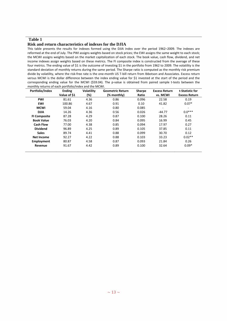
Table 1

Risk and return characteristics of indexes for the DJIA This table presents the results for indexes formed using the DJIA index over the period 1962–2009. The indexes are reformed at the end of July. The PWI assigns weights based on stock prices; the EWI assigns the same weight to each stock; the MCWI assigns weights based on the market capitalization of each stock. The book value, cash flow, dividend, and net income indexes assign weights based on these metrics. The FI composite index is constructed from the average of these four metrics. The ending value of $1 is the outcome of investing $1 in the portfolio from 1962 to 2009. The volatility is the standard deviation of monthly returns during the same period. The Sharpe ratio is computed as the monthly risk premium divide by volatility, where the risk-free rate is the one-month US T-bill return from Ibbotson and Associates. Excess return versus MCWI is the dollar difference between the index ending value for $1 invested at the start of the period and the corresponding ending value for the MCWI ($59.04). The p-value is obtained from paired sample t-tests between the monthly returns of each portfolio/index and the MCWI.

Portfolio/Index Ending Value of $1

Volatility (%)

Geometric Return (% monthly)

Sharpe Ratio

Excess Return vs. MCWI

t-Statistic for Excess Return

PWI 81.61 4.36 0.86 0.096 22.58 0.19 EWI 100.86 4.67 0.91 0.10 41.82 0.07*

MCWI 59.04 4.16 0.80 0.085 - - DJIA 14.26 4.36 0.56 0.026 -44.77 0.0***

FI Composite 87.28 4.29 0.87 0.100 28.26 0.11 Book Value 76.03 4.20 0.84 0.095 16.99 0.45 Cash Flow 77.00 4.38 0.85 0.094 17.97 0.27 Dividend 96.89 4.25 0.89 0.105 37.85 0.11

Sales 89.74 4.41 0.88 0.099 30.70 0.12 Net Income

Employment Revenue

92.27 80.87 91.67

4.22 4.58 4.42

0.88 0.87 0.89

0.103 0.093 0.100

33.23 21.84 32.64

0.02** 0.26

0.09*

~ 14 ~

Table 2 Fundamental indexes regressed on the Fama–French three-factor model This table discloses the results of the time series ordinary least squares regression analysis based on the Fama–French three-factor model as follows:

where RMt is for the Fama–French MCWI. The data are from January 1962 to December 2009. The coefficients , , and represent the sensitivity of share price changes against the change of the market risk, size, and value premiums, respectively. The intercept measures the excess return, which is unexplained by the loading on the risk factors. The superscripts ***, **, and * represent significance at the 1%, 5%, and 10% levels, respectively. The t-statistics for the coefficients are listed below the numbers. Adjusted R

2 values are in the final column.

Portfolio/Index α b S h Adj. R²

PWI 0 0.9749*** -0.2069*** 0.1665*** 0.902

-0.02 71.12 -10.8 7.99

EWI -0.0005 1.043*** -0.1435*** 0.2928*** 0.893

-0.73 67.98 -6.69 12.55

MCWI 0.0001 0.9221*** -0.285*** 0.0733*** 0.895

0.23 68.29 -15.1 3.57

DJIA -0.0031*** 0.9735*** -0.2043*** 0.1698*** 0.894

-5.05 68.15 -10.24 7.82

FI Composite -0.0004 0.9588*** -0.2337*** 0.3123*** 0.873

-0.67 62.47 -10.9 13.38

Book Value -0.0004 0.9126*** -0.2444*** 0.2865*** 0.822

-0.51 51.33 -9.83 10.6

Cash Flow -0.0006 0.9674*** -0.2362*** 0.2981*** 0.851

-0.8 57.03 -9.96 11.56

Dividend -0.0003 0.9383*** -0.2604*** 0.3459*** 0.844

-0.38 55.73 -11.06 13.51

Sales -0.0005 0.9799*** -0.1884*** 0.3118*** 0.869

-0.77 61.08 -8.4 12.78

Net Income 0.0003 0.9402*** -0.2674*** 0.1879*** 0.876

0.51 63.01 -12.82 8.28

Employment -0.0007 0.9899*** -0.1696*** 0.3066*** 0.825

-0.84 51.48 -6.31 10.49

Revenue -0.0004 0.984*** -0.1964*** 0.3021*** 0.871

-0.64 61.72 -8.81 12.46

𝑖𝑡 𝑓𝑡 = 𝑖 + 𝑖( 𝑡 𝑓𝑡) + 𝑖 𝑡 + 𝑖 𝑡 + 𝑖𝑡

~ 15 ~

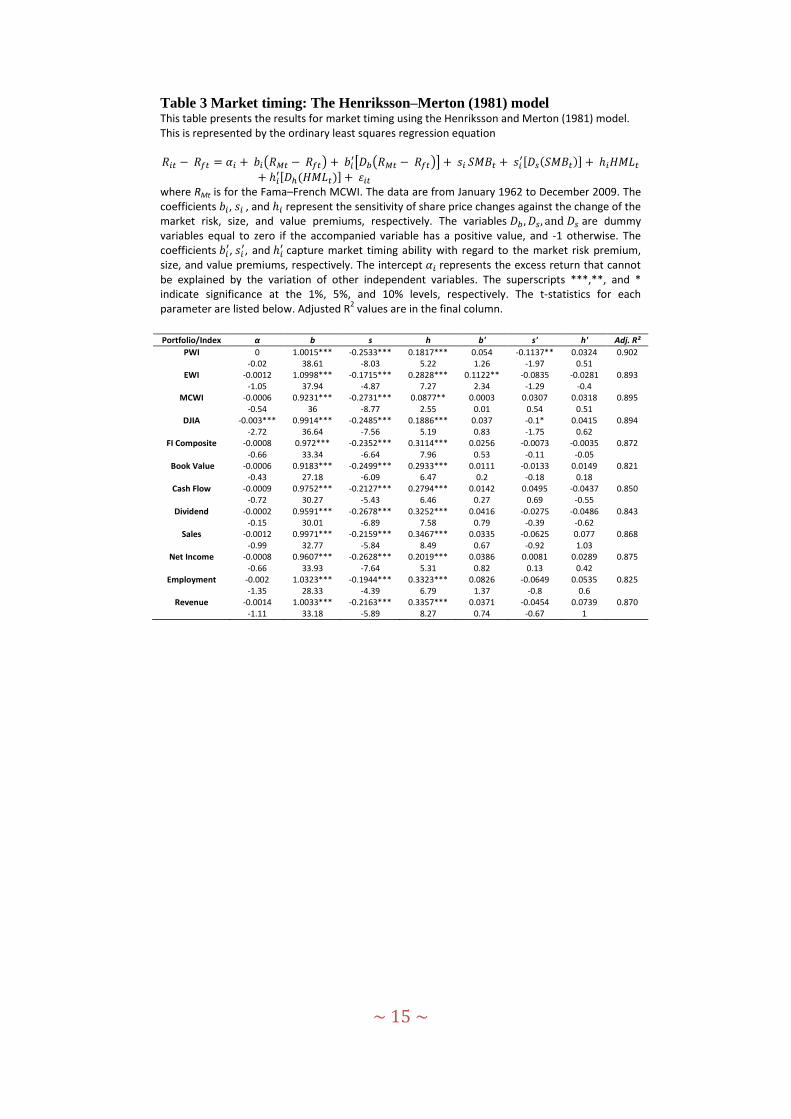
Table 3 Market timing: The Henriksson–Merton (1981) model This table presents the results for market timing using the Henriksson and Merton (1981) model. This is represented by the ordinary least squares regression equation

( ) [ ( )]

where RMt is for the Fama–French MCWI. The data are from January 1962 to December 2009. The coefficients , , and represent the sensitivity of share price changes against the change of the market risk, size, and value premiums, respectively. The variables are dummy variables equal to zero if the accompanied variable has a positive value, and -1 otherwise. The coefficients

, , and

capture market timing ability with regard to the market risk premium, size, and value premiums, respectively. The intercept represents the excess return that cannot be explained by the variation of other independent variables. The superscripts ***,**, and * indicate significance at the 1%, 5%, and 10% levels, respectively. The t-statistics for each parameter are listed below. Adjusted R

2 values are in the final column.

Portfolio/Index α b s h b' s' h' Adj. R²

PWI 0 1.0015*** -0.2533*** 0.1817*** 0.054 -0.1137** 0.0324 0.902

-0.02 38.61 -8.03 5.22 1.26 -1.97 0.51

EWI -0.0012 1.0998*** -0.1715*** 0.2828*** 0.1122** -0.0835 -0.0281 0.893

-1.05 37.94 -4.87 7.27 2.34 -1.29 -0.4

MCWI -0.0006 0.9231*** -0.2731*** 0.0877** 0.0003 0.0307 0.0318 0.895

-0.54 36 -8.77 2.55 0.01 0.54 0.51

DJIA -0.003*** 0.9914*** -0.2485*** 0.1886*** 0.037 -0.1* 0.0415 0.894

-2.72 36.64 -7.56 5.19 0.83 -1.75 0.62

FI Composite -0.0008 0.972*** -0.2352*** 0.3114*** 0.0256 -0.0073 -0.0035 0.872

-0.66 33.34 -6.64 7.96 0.53 -0.11 -0.05

Book Value -0.0006 0.9183*** -0.2499*** 0.2933*** 0.0111 -0.0133 0.0149 0.821

-0.43 27.18 -6.09 6.47 0.2 -0.18 0.18

Cash Flow -0.0009 0.9752*** -0.2127*** 0.2794*** 0.0142 0.0495 -0.0437 0.850

-0.72 30.27 -5.43 6.46 0.27 0.69 -0.55

Dividend -0.0002 0.9591*** -0.2678*** 0.3252*** 0.0416 -0.0275 -0.0486 0.843

-0.15 30.01 -6.89 7.58 0.79 -0.39 -0.62

Sales -0.0012 0.9971*** -0.2159*** 0.3467*** 0.0335 -0.0625 0.077 0.868

-0.99 32.77 -5.84 8.49 0.67 -0.92 1.03

Net Income -0.0008 0.9607*** -0.2628*** 0.2019*** 0.0386 0.0081 0.0289 0.875

-0.66 33.93 -7.64 5.31 0.82 0.13 0.42

Employment -0.002 1.0323*** -0.1944*** 0.3323*** 0.0826 -0.0649 0.0535 0.825

-1.35 28.33 -4.39 6.79 1.37 -0.8 0.6

Revenue -0.0014 1.0033*** -0.2163*** 0.3357*** 0.0371 -0.0454 0.0739 0.870 -1.11 33.18 -5.89 8.27 0.74 -0.67 1

~ 16 ~

Table 4

Crisis periods

This table partitions the time span into crisis and intermediate periods, indicating the name of

each period, start and end dates, and total duration. The boom periods are trough to peak, while

the bust periods are peak to trough on the DJIA.

Start Date

End Date

Years DJIA Start Date

DJIA End Date

Intermediate I Jan-62 Oct-71 9.8 700.0 839.0

Boom Nifty Fifty Nov-71 Nov-72 1.0 831.3 1018.2

Bust Nifty Fifty Dec-72 Dec-74 2.0 1020.0 616.2

Intermediate II Jan-75 Aug-86 11.6 703.7 1897.9

Boom 1987 Market Crash Sep-86 Jul-87 0.8 1767.9 2572.5

Bust 1987 Market Crash Aug-87 Nov-87 0.3 2661.5 1833.6

Intermediate III Dec-87 Jul-98 10.6 1937.0 8886.4

Boom Technology Bubble Aug-98 Dec-99 1.3 7544.0 11497.1

Bust Technology Bubble Jan-00 Aug-02 2.6 10941.8 8663.5

Intermediate IV Sep-02 Jan-06 3.3 7591.4 10864.7

Boom GFC Feb-06 Oct-07 1.7 10993.2 13930.4

Bust GFC Nov-07 Feb-09 1.3 13371.7 7062.9

Intermediate V Mar-09 Dec-09 0.8 7608.8 10428.0

~ 17 ~

Table 5 Returns (monthly compounded) earned by each index in each period.

Period Start End Years DJIA Start DJIA End PWI EWI MCWI DJIA FI BV C. F Div. SALES NI Employ. Rev.

Intermediate I Jan-62 Oct-71 9.75 700.0 839.0 66% 73% 64% 15% 63% 35% 58% 65% 83% 63% 73% 81%

Boom Nifty Fifty Nov-71 Nov-72 1.00 831.3 1018.2 26% 27% 29% 21% 28% 30% 29% 28% 27% 30% 25% 27%

Bust Nifty Fifty Dec-72 Dec-74 2.00 1020.0 616.2 -33% -31% -35% -39% -31% -27% -29% -30% -36% -31% -39% -37%

Intermediate II Jan-75 Aug-86 11.59 703.7 1897.9 467% 525% 434% 208% 565% 560% 558% 562% 575% 504% 528% 570%

Boom 1987 Market Crash Sep-86 Jul-87 0.83 1767.9 2572.5 40% 44% 36% 36% 40% 41% 39% 38% 41% 36% 38% 40%

Bust 1987 Market Crash Aug-87 Nov-87 0.25 2661.5 1833.6 -27% -30% -27% -29% -28% -28% -27% -26% -29% -28% -31% -29%

Intermedate III Dec-87 Jul-98 10.59 1937.0 8886.4 553% 570% 571% 385% 580% 593% 572% 557% 597% 615% 561% 593%

Boom Technology Bubble Aug-98 Dec-99 1.33 7544.0 11497.1 32% 29% 36% 29% 29% 28% 31% 21% 35% 33% 42% 38%

Bust Technology Bubble Jan-00 Aug-02 2.58 10941.8 8663.5 -20% -18% -33% -25% -16% -19% -19% -9% -17% -17% -18% -16%

Intermediate IV Sep-02 Jan-06 3.34 7591.4 10864.7 36% 43% 29% 25% 36% 38% 35% 37% 32% 36% 27% 33%

Boom GFC Feb-06 Oct-07 1.66 10993.2 13930.4 33% 36% 31% 28% 34% 30% 34% 39% 35% 30% 28% 33%

Bust GFC Nov-07 Feb-09 1.25 13371.7 7062.9 -46% -55% -47% -49% -59% -57% -62% -60% -56% -52% -45% -55%

Intermediate V Mar-09 Dec-09 0.75 7608.8 10428.0 52% 69% 46% 48% 62% 59% 68% 78% 46% 60% 49% 48%

~ 18 ~

Figure 1 FI outperformance compared with FI size and value ‘tilts’. The solid and sashed lines show the difference between the FI composite and the

MCWI size and value coefficients (RHS axis), and beneath them is the curve of the accumulated outperformance (compounding) of the FI

composite index against the MCWI (LHS axis). The crisis periods are shaded darker.

-0.5

-0.4

-0.3

-0.2

-0.1

0

0.1

0.2

0.3

0.4

0.5

-10%

0%

10%

20%

30%

40%

50%

60%

70%

80%1

96

61

96

71

96

81

96

91

97

01

97

11

97

21

97

31

97

41

97

51

97

61

97

71

97

81

97

91

98

01

98

11

98

21

98

31

98

41

98

51

98

61

98

71

98

81

98

91

99

01

99

11

99

21

99

31

99

41

99

51

99

61

99

71

99

81

99

92

00

02

00

12

00

22

00

32

00

42

00

52

00

62

00

72

00

82

00

9

Tilt

Re

turn

h tilt 48 s tilt 48

~ 19 ~

Figure 2 (a) Stock weighting for the FI composite and MCWI in August 1998 (start of the technology boom)

~ 20 ~

Figure 2 (b) Stock weighting for the FI composite and MCWI in December 1999 (height of the technology bubble)

~ 21 ~

Figure 3 (a) Stock weighting for the FI composite and MCWI in October 2007 (start of the global financial crisis).

~ 22 ~

Figure 3 (b) Stock weighting for the composite and market cap indexes in February 2009 (end of the global financial crisis bust period).