1 Is the Demographic Transition Causing an Increase in Income Inequality? Evidence from Taiwan by Andrew Mason and Sang-Hyop Lee 1 November 24, 2002 As the demographic transition has proceeded in countries around the world, attention has increasingly focused on the economic implications of population aging. Perhaps no issue has received more attention than the sustainability of public old-age security programs that have promised substantial transfers to seniors living in Japan, the West, and many developing countries in Latin America. How public transfer systems are reformed in response to demographic pressure will have important and lasting implications for levels of poverty and inequality. In Asia the extended family is a much more important component of the old-age support system than in the West. In some of the most developed Asian countries about half of all seniors live with adult children. In many other Asian countries a much higher percentage of seniors live in multi-generation extended households. As the demographic transition proceeds and Asia’s populations age, the family support system will be subject to the same pressures as public support systems. Adult children may find that they are supporting their parents for more years and that they have fewer siblings with whom they can share the burden of old-age support. Alternatively seniors may find that the family support provided in the past is no longer forthcoming. How family support systems evolve is no less important than how public programs are reformed in response to demographic pressure. These issues are especially pressing in Taiwan and other Asian countries that have experienced unusually rapid demographic transitions. As a consequence population aging will be especially rapid and the pressure on support systems particularly severe. Although the implications of population aging for the family support system has received relatively little attention, the implications of aging for income inequality in Taiwan and elsewhere has been the subject of several important studies. A consensus has not been reached as to whether aging leads to a rise or a decline in inequality in Taiwan. Liu (1978) concludes that changes in the distributions of age of household head and 1 The authors are Professor of Economics, University of Hawaii at Manoa and Senior Fellow, East-West Center and Assistant Professor of Economics, University of Hawaii at Manoa, respectively. Earlier versions of this paper were presented at the Workshop on Population and Macroeconomics at the Max Planck Institute in Rostock, Germany and at the Bay Area Consortium on Population Seminar and we received many useful suggestions from those participants and our colleagues in Hawaii. Our thanks to Turro Wongkaren for his able research assistance. For additional information please contact [email protected]. The authors gratefully acknowledge the support of the Rockefeller Foundation.
Transcript
1
Is the Demographic Transition Causing an Increase in Income Inequality? Evidence from Taiwan
by
Andrew Mason and Sang-Hyop Lee1 November 24, 2002
As the demographic transition has proceeded in countries around the world, attention has increasingly focused on the economic implications of population aging. Perhaps no issue has received more attention than the sustainability of public old-age security programs that have promised substantial transfers to seniors living in Japan, the West, and many developing countries in Latin America. How public transfer systems are reformed in response to demographic pressure will have important and lasting implications for levels of poverty and inequality. In Asia the extended family is a much more important component of the old-age support system than in the West. In some of the most developed Asian countries about half of all seniors live with adult children. In many other Asian countries a much higher percentage of seniors live in multi-generation extended households. As the demographic transition proceeds and Asia’s populations age, the family support system will be subject to the same pressures as public support systems. Adult children may find that they are supporting their parents for more years and that they have fewer siblings with whom they can share the burden of old-age support. Alternatively seniors may find that the family support provided in the past is no longer forthcoming. How family support systems evolve is no less important than how public programs are reformed in response to demographic pressure. These issues are especially pressing in Taiwan and other Asian countries that have experienced unusually rapid demographic transitions. As a consequence population aging will be especially rapid and the pressure on support systems particularly severe. Although the implications of population aging for the family support system has received relatively little attention, the implications of aging for income inequality in Taiwan and elsewhere has been the subject of several important studies. A consensus has not been reached as to whether aging leads to a rise or a decline in inequality in Taiwan. Liu (1978) concludes that changes in the distributions of age of household head and
1 The authors are Professor of Economics, University of Hawaii at Manoa and Senior Fellow, East-West Center and Assistant Professor of Economics, University of Hawaii at Manoa, respectively. Earlier versions of this paper were presented at the Workshop on Population and Macroeconomics at the Max Planck Institute in Rostock, Germany and at the Bay Area Consortium on Population Seminar and we received many useful suggestions from those participants and our colleagues in Hawaii. Our thanks to Turro Wongkaren for his able research assistance. For additional information please contact [email protected]. The authors gratefully acknowledge the support of the Rockefeller Foundation.
2
household size were important contributors to a decline in inequality between 1964 and 1970. Chu (1997) examines the effects of age structure on family income using the Gini coefficient and shows that changes in Taiwan’s demography reduced the inequality in family earnings between 1980 and 1990. In contrast, Deaton and Paxson (1997) concludes that aging is leading to greater inequality in household consumption and Schultz (1997) concludes that aging is leading to an increase in inequality in income per adult. These studies do not consider, however, how population aging is influencing living arrangements. Their focus is on the compositional effects of aging. The analysis presented in this paper is based on a model of population aging and per capita income inequality that explicitly incorporates the effects of aging on the prevalence of multi-generation extended households (Mason and Lee 2002) (Lee and Mason 2002). Based on analysis of Taiwan’s experience from 1978 to 1998, we conclude that population aging has led to an increase in the proportion of non-senior adults living with their parents. Because of the increased extent to which incomes are being pooled, population aging has led to a decline in income inequality in Taiwan. A Model of Income Inequality Analysis is facilitated using a model that captures key features of the links between age structure, living arrangements, and inequality. The model abstracts from some issues that are potentially important, as will be discussed below. The use of a highly stylized model, however, allows us to focus on the changes in inequality when the population is aging and, thereby, influencing both the age composition of the population and the extent to which families are pooling their incomes by establishing multi-generational extended households.
The population we consider consists of one sex and two generations or age groups. The young members of the population are non-senior adults or non-seniors for short. The old members of the population, seniors, are the parents of non-senior adults. The population of non-seniors is designated by K, seniors by P, and the total population by M=K+P. The age structure of the population is measured in one of two ways, either by the dependency ratio, /D P K= , or by the share of non-seniors or seniors in the total population. The proportion of the adult population who are non-seniors is
1/(1 ),km D= + and the proportion of the adult population who are seniors is
/(1 ).pm D D= +
Individuals form either nuclear or extended households. Nuclear households consist of one member, either a non-senior or a senior. Extended households consist of one non-senior member and xD senior members where xD can take on fractional values.
xD is the dependency ratio within extended households. The subscripts n and x are used
to distinguish the nuclear and extended populations; hence, xK and nK represent the
total number of non-seniors living in extended and nuclear households, respectively. The proportion of individuals living in an extended household is designated by x and the
3
proportion living in a nuclear household by n. The proportion of non-seniors living in an extended household is kx ; the proportion of seniors living in extended households is .px
The mean incomes of non-seniors and seniors are designated by kY and pY , respectively, and the variances by ( )kV Y and ( )pV Y , respectively. The co-variance
between the income of non-seniors and seniors within extended household is ( )k pC Y Y . When individuals form extended households they fully pool their income. Hence,
we do not consider any intra-household distributional issues. Per capita household income is designated by Y, mean per capita household income by Y , and the variance in per capita household income by V(Y).2 Except as noted, income inequality is measured by the variance in per capita household income.
Previous studies of age composition and inequality have shown that the
relationship between age structure and the variance of per capita household income consists of two components: a difference in variances effect and a difference in means effect. The difference in variances effect arises because the variance in incomes varies by age. Changes in the age-composition of the population that increase the representation of age groups with high income variance leads to higher income variance for the population. The difference in means effect arises because mean income varies by age. Changes in the age composition of the population that increase the representation of age groups with mean income substantially different from the grand mean (or the mean income of other age groups) leads to greater income inequality (Lam 1997).
Lee and Mason (2002) generalize the age-inequality model to incorporate the
effects of extended living arrangements. We make several key assumptions that simplify the analysis considerably. We assume that the choice of living arrangements is independent of income and that the dependency ratio within extended households is independent of the income of the household members. Under these simplifying assumptions, the variance of income is given by equation (1.1). The difference in variances component is a weighted average of the first three right-hand-side terms in equation (1.1): the variance of the per capita income of non-seniors, the variance of the per capita income of seniors, and the co-variance between the income of co-residing seniors and non-seniors.3 The difference in means component is the fourth right-hand-side term in equation (1.1):
2
1 2 3 4( ) ( ) ( ) ( ) ( )k p k p k pV Y wV Y w V Y w C Y Y w Y Y= + + + − (1.1)
where:
2 The variance in income is calculated using the number of household members as weights as is standard in the literature on income inequality. Studies of earnings inequality frequently use the variance in the log of earnings to measure inequality, but the natural income of income is undefined for persons with no incomes or losses for the year. 3 The first three coefficients sum to 1.
4
1
2
3
24
0
0
2 0
( ) 0.
k k px x x
p k px x x
k px x x
k p p pn n n n x n x
w m m m m
w m m m m
w m m m
w m m m m m m m
= − >
= − >
= >
= + − >
(1.2)
The variables xm and nm are the proportions of adults living in extended and nuclear
households, respectively; km and pm are the proportions of adults who are non-seniors and seniors, respectively; k
xm and pxm are the proportions of extended household adult
members who are non-seniors and seniors, respectively; and, knm and p
nm are the
proportions of nuclear household adult members who are non-seniors and seniors, respectively.
If all adults lived in nuclear households, the inequality model is greatly simplified. The coefficients reduce to:
1
2
3
4
0
.
k
p
k p
w m
w m
w
w m m
=
==
=
(1.3)
In the simple model, the difference in variances effect is a weighted average of the variances of non-senior and senior incomes where the weights are the proportion of the population belonging to the non-senior and senior age groups. The difference in means effect is non-monotonic in age structure reaching a peak when the population is equally divided between the non-senior and senior age groups.
In the extended household model, the difference in variances effect, captured by the first three terms in equation (1.2), depends on the extent to which members in the population pool their income as measured by k p
x x xm m m . The variances of individual
incomes carry a smaller weight and the co-variance term carries a larger weight the greater the extent of income pooling. If the co-variance of the income of co-resident seniors and non-seniors is negative, it is obvious that V(Y) is reduced by greater pooling, i.e., an increase in the coefficient of the co-variance term. But even if there is a high positive correlation between the income of co-resident seniors and non-seniors, the effect of pooling is to reduce the variance in per capita income.4
The extent of income pooling, k p
x x xm m m , increases with the proportion of adults in
extended households and balance between seniors and non-senior members within extended households. Given the proportion of adults in extended households, the pooling 4 See Lee and Mason 2000 for a formal derivation. Also Lam 1997 shows that pooling of incomes will reduce the coefficient of variation if the correlation is less than perfect.
5
term reaches a maximum when extended households consist of equal numbers of seniors and non-seniors, i.e., 0.5k p
x xm m= = .
Suppose that the extent of pooling were unaffected by population aging. In this
case, the difference in variances effect of aging would be independent of the extent of co-residence. The effect of an increase in the proportion senior is given by
( ) / ( ) ( )p p kV Y m V Y V Y∂ ∂ = − . As we shall see in the next section, however, aging does have an important effect on the extent of pooling and the variance in income beyond that captured by the simpler specification.
The difference in means effect is captured by the last term in equation (1.1). The first additive term in 4w captures the effect of the differences in the mean income of non-senior and senior nuclear households. The effect is larger the larger the proportion of persons living in nuclear households and the greater the balance in non-senior and senior households. The second additive term in 4w captures the effect of differences in the mean income of nuclear and extended households. If the population shares of seniors in nuclear and extended households are equal, the mean incomes of extended and nuclear households will also be equal, and this term drops out.5 The greater the difference in the population shares of seniors, as captured by 2( )p p
n xm m− , the greater the difference in the
mean incomes of nuclear and extended households and the greater the difference in means effect. The effect also increases the greater the balance in the proportion of the population in nuclear and extended households as captured by n xm m .
Equation (1.1) is applied to the analysis of aging on income inequality by holding
the characteristics of the income of seniors and non-seniors constant at observed levels and varying the weights. As we shall see, however, changes in age structure influence the weights directly as measured by km and pm but also by influencing living arrangements. Aging and Living Arrangements The model of living arrangements incorporates the effects of aging in two distinctive ways. The first effect explored is that improvements in health, which lead to higher survival rates and population aging, may also lead to an increase in the extent to which seniors maintain separate households. If this effect is important, it would be a source of greater income inequality as explained above.
The second effect is that changes in age structure influence the availability of kin. An increase in the relative number of seniors in a population increases the relative number of surviving parents with whom non-senior adults may establish extended households. If the increased availability of seniors leads to a rise in extended households, this will serve to reduce income inequality.
5 This follows given our assumption that living arrangements are independent of income.
6
A simple specification taken from Mason and Lee (2002) is used to estimate the
effects of survival on living arrangements among seniors, defined as persons aged 60 and older. The proportion of seniors aged a living in nuclear households in year t ( ( , )n a t ) depends on two cohort variables and an age variable. The cohort variables capture persistent characteristics of members of each birth cohort. The first variable, the year of birth or ( )BYear t a− , is included to capture the effects of broad social and economic trends that may be influencing the extent to which seniors are choosing to live independently from their offspring. The second cohort variable, the sex ratio at age 60 or
( )SexRatio t a− , is included to capture the effects of large imbalances in the sex ratio that influenced the extent to which cohort members married and produced offspring. This is an important and unusual feature of Taiwan’s demography because it experienced large-scale, disproportionately male immigration from mainland China circa 1950. Note that cohort variables are indexed only by year of birth, t a− . The effect of survival is incorporated into the model using age-specific survival rates, ( , )s a t . We use the log-odds of the proportion nuclear as the dependent variable so as to constrain the values of the proportion nuclear to between 0 and 1:6
0 1 2 3
( , )ln ( ) ( ) ln ( , ) for 60.
1 ( , )
n a tBYear t a SexRatio t a s a t a
n a tβ β β β
= + − + − + ≥ −
(1.4)
Given the proportion of seniors living in extended households, the
proportion of non-seniors (30 60)a≤ < living in extended households may increase with a rise in the population dependency ratio, i.e, with an increase in the availability of senior kin. The effect is not a deterministic one, however, because a second possibility is that an increase in the dependency ratio will produce a rise in the dependency ratio within extended households.
The intergenerational demographic connections that influence extended living
arrangements are modeled using an approach that in most respects is identical to the highly stylized model used to model income inequality in the preceding section. We continue to focus only on the adult population, which again is divided into two generations – non-seniors and seniors. The senior and non-senior populations, however, consist of multiple age groups.7 If N(a,t) is the population aged a in year t, then those groups for which 2g a g≤ < are classified as non-seniors and those for which 2a g≥ are classified as seniors. We assume that all births occur at age g. Hence, at any point in time individuals aged a have parents aged a+g. N(a) is the population aged a and N(a+g) is both the population aged a+g and the parents of persons aged a.8 Extended
6 There may be time effects as well. For example, fluctuations in the unemployment rate may influence the extent of co-residence for all birth cohorts and age groups. The analysis here is concerned with long run trends, however, and the effects of annual fluctuations are absorbed in the error term in the statistical analysis presented below. 7 In the empirical section we use single-year age groups with those aged 30-59 classified as non-seniors and those 60 and older classified as seniors. 8 Some individuals in the a+g age group may not be parents.
7
households are formed when persons aged a and persons aged a+g choose to live together.
The intergenerational demographic connections are captured by the following identity:
( , ) ( , ) ( , ) for a<2g,x a t ddx a t x a g t≡ + (1.5) where:
( , ) ( , ) / ( , ),
( , ) ( , ) / ( , ), and
( , ) ( , ) / ( , ) for 2 .
x
x x x
ddx a t D a t D a t
D a t N a g t N a t
D a t N a g t N a t g a g
== +
= + ≤ <
(1.6)
The interdependence between the proportion of seniors and non-seniors living in extended households is incorporated into the analysis using age-specific dependency ratios that approximate the age structure of families and extended households. The age in this formulation is the age of the non-senior members of the family and/or the extended household. Equation (1.5) is particularly important to our analysis of income inequality because it shows that population aging will lead to changes in the extent of pooling. Given the proportion of seniors living in extended households, an increase in D must produce either an increase in the proportion of non-seniors living in extended households or an increase in /x p k
x xD m m= . In either event, the extent of pooling will change.
Mason and Lee (2002) provides a more detailed and formal treatment of the
relationship between the relative dependency structure in the population (ddx), the demographic transition, and the form of extended living arrangements. Here, we confine ourselves to a simpler empirical strategy that allows us to analyze the effects of aging on living arrangements and to test a key issue – whether changes in the dependency ratio in extended households match, in percentage terms, changes in the population dependency ratio. If they do, then aging does not lead to a rise in the proportion of non-seniors living in extended households. The model we estimate below is:
59
30
ln ( , ) ( ) ( , ) ln ( , ).x
a
D a t a Age a t D a tα β=
= +∑ (1.7)
The variables Age(a) are dummy variables that take the value of 1 depending on the current age of the cohort in question. If the coefficient β is significantly less than one, it follows that the increased availability of seniors in the population is leading to a rise in the proportion of non-seniors living in extended households.
8
Empirical Analysis Data We use the Survey of Family Income and Expenditure in Taiwan (FIES, also known as the Survey of Personal Income Distribution in Taiwan until 1993). The FIES was first conducted in 1964 and, then, every other year until 1970. Since then, the survey has been conducted annually and data are available for the 1976 and subsequent surveys. For technical reasons, we have confined our analysis to surveys conducted in 1978 and later until 1998. The number of household surveyed has varied over time, but the sample size is more than sufficient for our purposes. In 1998, about 0.4 percent of all households (14,031 households and 52,610 individuals) were covered. These are not panel data, but repeated cross-sections. There are two features of the FIES that are important to the analysis presented below. First, the FIES has a complete household roster with age, sex, relationship to head, and other individual characteristics of household members. The household roster is used to partition households into groups of individuals belonging to the same generation and to define nuclear and extended households. For example, the head, spouse of the head, or sibling of the head would belong to one generation. The mother, father, aunt, or uncle of the head would belong to a different generation. All individuals who are related to the head are assigned to a generation. Extended households are defined as households consisting of two or more generations in which at least one member is 30 years of age or older. Note that marital status has no bearing on our definition of household type. The second feature of the FIES is that household income is assigned to members of the household. Although there is a residual category for income that cannot be assigned to an individual, this category is rarely used. Consequently, we can calculate income characteristics separately for the non-senior and senior generation within extended households. Income is measured by total current income excluding depreciation. We analyze income per adult. All means and variances are weighted by the number of adults in the household or sub-unit.9
Nuclear households are designated as senior households or non-senior households based on the age of the primary income earner. If he or she is 60 or older the household is classified as senior. In extended households, the adult members are classified as senior or non-senior based on the generation to which they belong. The members of the youngest adult generation in the household are designated as non-senior adults; the members of all other adult generations are designated as senior adults.
The survey data are used to construct estimates of the means and variances of the income of seniors and non-seniors in equation (1.1). V(Y) for seniors and non-seniors is calculated as the variance in household income per senior or non-senior using the number
9 For a discussion of some of the issues that arise in measuring income inequality see Lam 1997 or Schultz 1997.
9
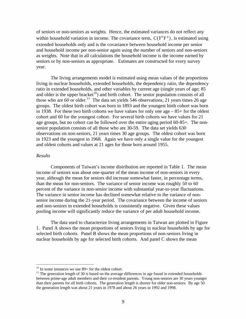
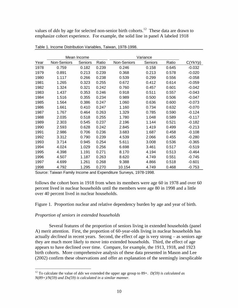
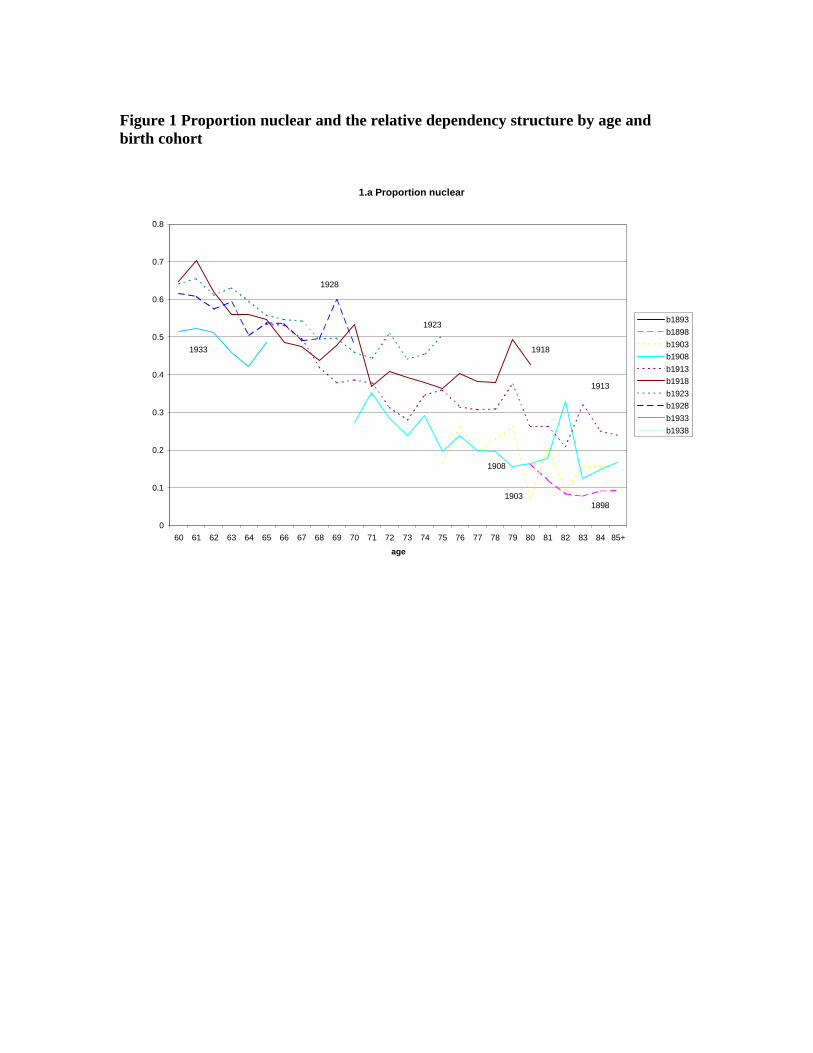
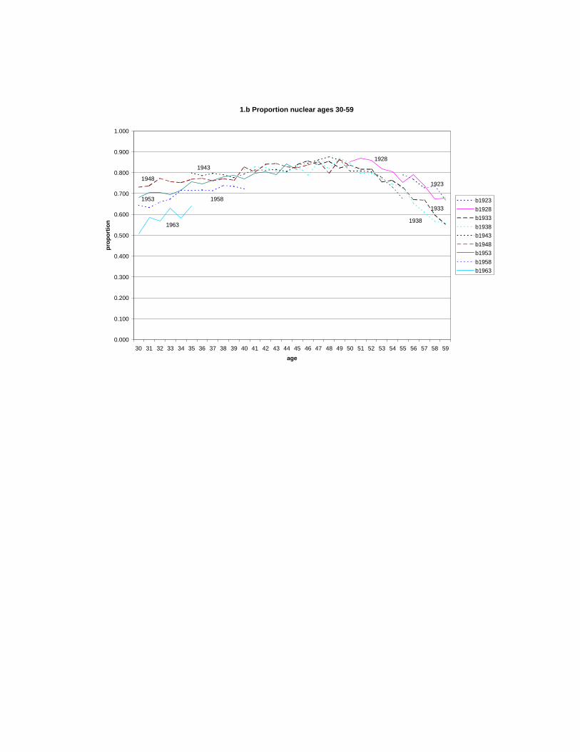
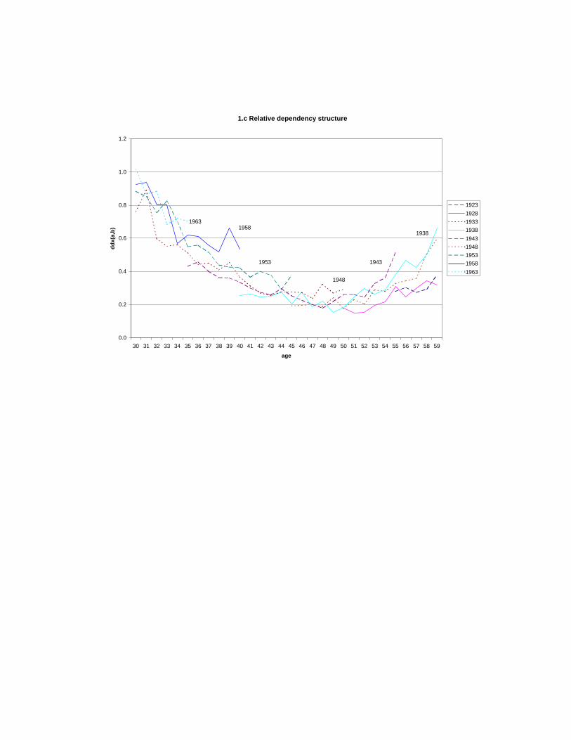
of seniors or non-seniors as weights. Hence, the estimated variances do not reflect any within household variation in income. The covariance term, ( )k pC Y Y , is estimated using extended households only and is the covariance between household income per senior and household income per non-senior again using the number of seniors and non-seniors as weights. Note that in all calculations the household income is the income earned by seniors or by non-seniors as appropriate. Estimates are constructed for every survey year. The living arrangements model is estimated using mean values of the proportions living in nuclear households, extended households, the dependency ratio, the dependency ratio in extended households, and other variables by current age (single years of age; 85 and older is the upper bracket10) and birth cohort. The senior population consists of all those who are 60 or older.11 The data set yields 546 observations, 21 years times 26 age groups. The oldest birth cohort was born in 1893 and the youngest birth cohort was born in 1938. For these two birth cohorts we have values for only one age – 85+ for the oldest cohort and 60 for the youngest cohort. For several birth cohorts we have values for 21 age groups, but no cohort can be followed over the entire aging period 60-85+. The non-senior population consists of all those who are 30-59. The data set yields 630 observations on non-seniors, 21 years times 30 age groups. The oldest cohort was born in 1923 and the youngest in 1968. Again we have only a single value for the youngest and oldest cohorts and values at 21 ages for those born around 1955. Results Components of Taiwan’s income distribution are reported in Table 1. The mean income of seniors was about one-quarter of the mean income of non-seniors in every year, although the mean for seniors did increase somewhat faster, in percentage terms, than the mean for non-seniors. The variance of senior income was roughly 50 to 60 percent of the variance in non-senior income with substantial year-to-year fluctuations. The variance in senior income has declined somewhat relative to the variance of non-senior income during the 21-year period. The covariance between the income of seniors and non-seniors in extended households is consistently negative. Given these values pooling income will significantly reduce the variance of per adult household income. The data used to characterize living arrangements in Taiwan are plotted in Figure 1. Panel A shows the mean proportions of seniors living in nuclear households by age for selected birth cohorts. Panel B shows the mean proportions of non-seniors living in nuclear households by age for selected birth cohorts. And panel C shows the mean
10 In some instances we use 89+ for the oldest cohort. 11 The generation length of 30 is based on the average differences in age found in extended households between prime-age adult members and their co-resident parents. Young non-seniors are 30 years younger than their parents for all birth cohorts. The generation length is shorter for older non-seniors. By age 50 the generation length was about 21 years in 1978 and about 26 years in 1992 and 1998.
10
values of ddx by age for selected non-senior birth cohorts.12 These data are drawn to emphasize cohort experience. For example, the solid line in panel A labeled 1918 Table 1. Income Distribution Variables, Taiwan, 1978-1998. Mean Income Variance Year Non-Seniors Seniors Ratio Non-Seniors Seniors Ratio C(YkYp) 1978 0.759 0.182 0.239 0.246 0.158 0.645 -0.032 1979 0.891 0.213 0.239 0.368 0.213 0.578 -0.020 1980 1.117 0.266 0.238 0.539 0.299 0.556 -0.058 1981 1.265 0.323 0.255 0.672 0.412 0.614 -0.059 1982 1.324 0.321 0.242 0.760 0.457 0.601 -0.042 1983 1.437 0.353 0.246 0.918 0.511 0.557 -0.043 1984 1.516 0.355 0.234 0.989 0.500 0.506 -0.047 1985 1.564 0.386 0.247 1.060 0.636 0.600 -0.073 1986 1.661 0.410 0.247 1.160 0.734 0.632 -0.070 1987 1.767 0.464 0.263 1.329 0.785 0.590 -0.124 1988 2.035 0.518 0.255 1.780 1.048 0.589 -0.117 1989 2.303 0.545 0.237 2.196 1.144 0.521 -0.182 1990 2.593 0.628 0.242 2.845 1.419 0.499 -0.213 1991 2.986 0.706 0.236 3.683 1.687 0.458 -0.108 1992 3.312 0.790 0.239 4.539 2.066 0.455 -0.280 1993 3.714 0.945 0.254 5.611 3.008 0.536 -0.365 1994 4.024 1.029 0.256 6.698 3.461 0.517 -0.519 1995 4.398 1.191 0.271 8.170 4.194 0.513 -0.464 1996 4.507 1.187 0.263 8.620 4.749 0.551 -0.745 1997 4.699 1.261 0.268 9.388 4.866 0.518 -0.601 1998 4.792 1.295 0.270 10.154 4.749 0.468 -0.753 Source: Taiwan Family Income and Expenditure Surveys, 1978-1998. follows the cohort born in 1918 from when its members were age 60 in 1978 and over 60 percent lived in nuclear households until the members were age 80 in 1998 and a little over 40 percent lived in nuclear households. Figure 1. Proportion nuclear and relative dependency burden by age and year of birth. Proportion of seniors in extended households Several features of the proportion of seniors living in extended households (panel A) merit attention. First, the proportion of 60-year-olds living in nuclear households has actually declined in recent years. Second, the effect of age is very strong – as seniors age they are much more likely to move into extended households. Third, the effect of age appears to have declined over time. Compare, for example, the 1913, 1918, and 1923 birth cohorts. More comprehensive analysis of these data presented in Mason and Lee (2002) confirm these observations and offer an explanation of the seemingly inexplicable
12 To calculate the value of ddx we extended the upper age group to 89+. D(59) is calculated as N(89+)/N(59) and Dx(59) is calculated in a similar manner.
11
decline in the proportion of young seniors living in nuclear households. The proportion of young seniors living in nuclear households was temporarily elevated by the large surplus of males. The sex ratio exceeded 140 males per 100 females for the cohorts born in the mid- and late-1920s. Many men did not marry and raise children and, hence, could not establish extended households. By the time we reach the 1938 birth cohort, however, the sex ratio at age 60 had dropped to a more normal level somewhat below 100. These aspects of the proportion of non-seniors living in extended households are captured using the regression model, equation (1.4), described in more detail above. The model was estimated using the consistent variance-covariance matrix estimator of White (1980). The standard errors are thus robust to heteroscedasticity. The estimated results with standard errors presented in parentheses are:
2
ln( /(1 )) 56.13 1.46 0.028 8.16ln
(3.77) (0.076) (0.02) (0.50)
N=546 R 0.86
n n SexRatio BYear s− = − + + +
=
(1.8)
The sex ratio has a strong positive effect on the proportion of any cohort living in nuclear households. Controlling for the sex ratio the coefficient of birth year is significantly greater than zero. Over time there has been a gradual shift away from the extended family in Taiwan that has been masked by the large swings in the sex ratio. The model does not identify the source of the trend toward nuclear households. It may be increased income, higher educational attainment, urbanization, improvements in the non-family social support system, or other factors. Although any of these variables could in principle be used as regressors in the model, we do not think the model has sufficient power to distinguish among these alternative explanations using the data that are available. The natural logarithm of the age-specific survival rate captures the influences of individual aging on the probability that a senior will live with an adult child. At any point in time age groups with a lower risk of death – those at younger ages – are more likely to live in nuclear households. Over time the survival rate at any given age is rising, producing an increase in the proportion living in nuclear households at each age. The shift in the age effect is consistent with Taiwan’s experience as shown in Figure 1. However, the regression model tends to underestimate the shift in the age effects (Mason and Lee 2002). The Relative dependency structure (ddx)
The model of living arrangements is completed by estimating the effect of changes in the population dependency ratios on the dependency ratios in extended households. Equation (1.7) is estimated using ordinary least-squares regression. The age dummy coefficients are available from the authors. The estimated equation, with standard error in parentheses, is:
12
59
30
2
ˆln ( , ) ( ) ( ) 0.588ln ( , ).
(0.018)
630 0.967
x
a
D a t a Age a D a t
N R
α=
= +
= =
∑ (1.9)
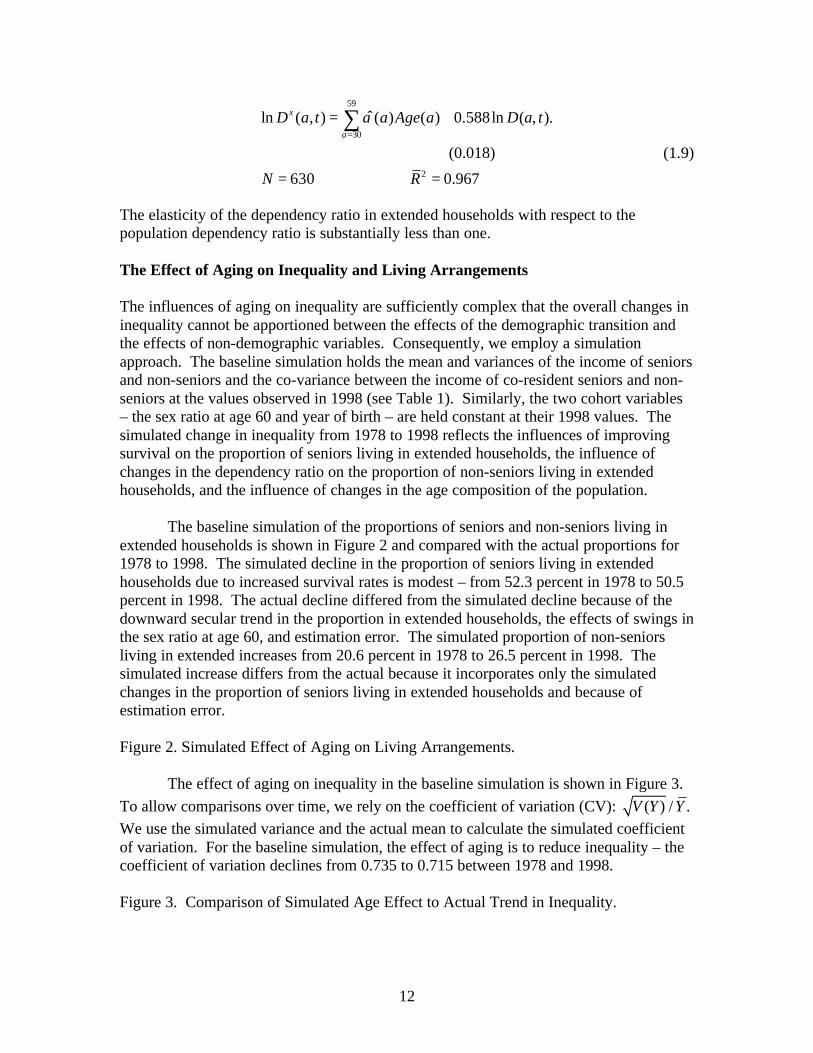
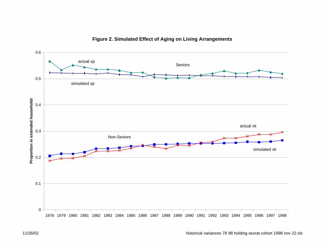
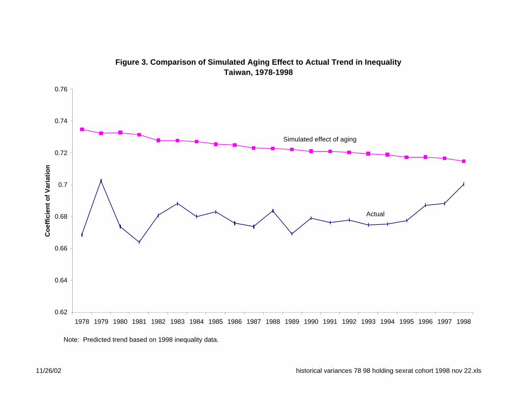
The elasticity of the dependency ratio in extended households with respect to the population dependency ratio is substantially less than one. The Effect of Aging on Inequality and Living Arrangements The influences of aging on inequality are sufficiently complex that the overall changes in inequality cannot be apportioned between the effects of the demographic transition and the effects of non-demographic variables. Consequently, we employ a simulation approach. The baseline simulation holds the mean and variances of the income of seniors and non-seniors and the co-variance between the income of co-resident seniors and non-seniors at the values observed in 1998 (see Table 1). Similarly, the two cohort variables – the sex ratio at age 60 and year of birth – are held constant at their 1998 values. The simulated change in inequality from 1978 to 1998 reflects the influences of improving survival on the proportion of seniors living in extended households, the influence of changes in the dependency ratio on the proportion of non-seniors living in extended households, and the influence of changes in the age composition of the population. The baseline simulation of the proportions of seniors and non-seniors living in extended households is shown in Figure 2 and compared with the actual proportions for 1978 to 1998. The simulated decline in the proportion of seniors living in extended households due to increased survival rates is modest – from 52.3 percent in 1978 to 50.5 percent in 1998. The actual decline differed from the simulated decline because of the downward secular trend in the proportion in extended households, the effects of swings in the sex ratio at age 60, and estimation error. The simulated proportion of non-seniors living in extended increases from 20.6 percent in 1978 to 26.5 percent in 1998. The simulated increase differs from the actual because it incorporates only the simulated changes in the proportion of seniors living in extended households and because of estimation error. Figure 2. Simulated Effect of Aging on Living Arrangements. The effect of aging on inequality in the baseline simulation is shown in Figure 3.
To allow comparisons over time, we rely on the coefficient of variation (CV): ( ) / .V Y Y
We use the simulated variance and the actual mean to calculate the simulated coefficient of variation. For the baseline simulation, the effect of aging is to reduce inequality – the coefficient of variation declines from 0.735 to 0.715 between 1978 and 1998. Figure 3. Comparison of Simulated Age Effect to Actual Trend in Inequality.
13
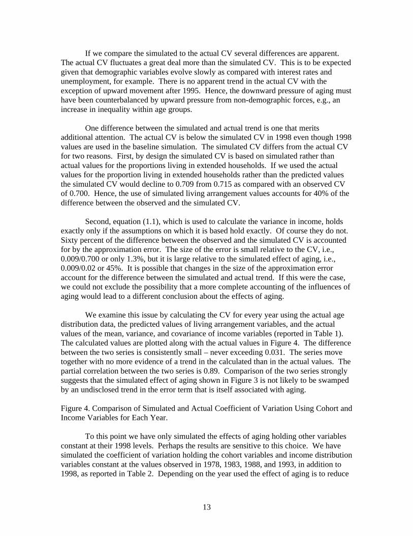
If we compare the simulated to the actual CV several differences are apparent. The actual CV fluctuates a great deal more than the simulated CV. This is to be expected given that demographic variables evolve slowly as compared with interest rates and unemployment, for example. There is no apparent trend in the actual CV with the exception of upward movement after 1995. Hence, the downward pressure of aging must have been counterbalanced by upward pressure from non-demographic forces, e.g., an increase in inequality within age groups.
One difference between the simulated and actual trend is one that merits additional attention. The actual CV is below the simulated CV in 1998 even though 1998 values are used in the baseline simulation. The simulated CV differs from the actual CV for two reasons. First, by design the simulated CV is based on simulated rather than actual values for the proportions living in extended households. If we used the actual values for the proportion living in extended households rather than the predicted values the simulated CV would decline to 0.709 from 0.715 as compared with an observed CV of 0.700. Hence, the use of simulated living arrangement values accounts for 40% of the difference between the observed and the simulated CV.
Second, equation (1.1), which is used to calculate the variance in income, holds exactly only if the assumptions on which it is based hold exactly. Of course they do not. Sixty percent of the difference between the observed and the simulated CV is accounted for by the approximation error. The size of the error is small relative to the CV, i.e., 0.009/0.700 or only 1.3%, but it is large relative to the simulated effect of aging, i.e., 0.009/0.02 or 45%. It is possible that changes in the size of the approximation error account for the difference between the simulated and actual trend. If this were the case, we could not exclude the possibility that a more complete accounting of the influences of aging would lead to a different conclusion about the effects of aging.
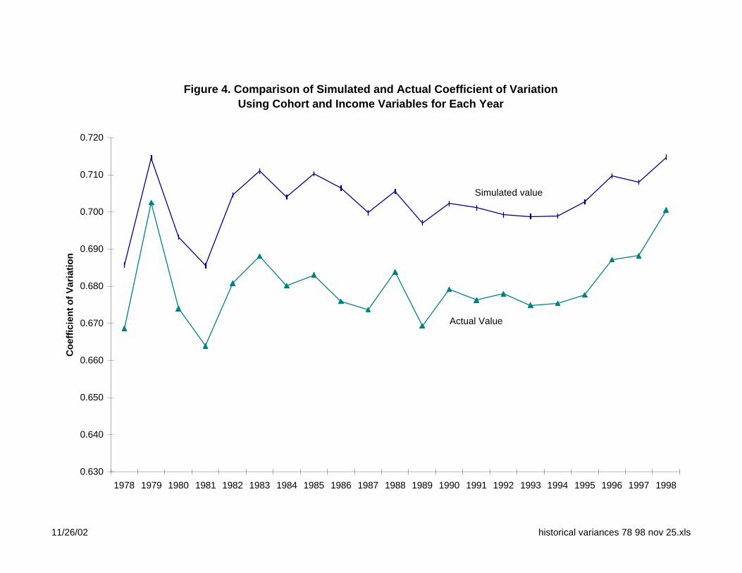
We examine this issue by calculating the CV for every year using the actual age distribution data, the predicted values of living arrangement variables, and the actual values of the mean, variance, and covariance of income variables (reported in Table 1). The calculated values are plotted along with the actual values in Figure 4. The difference between the two series is consistently small – never exceeding 0.031. The series move together with no more evidence of a trend in the calculated than in the actual values. The partial correlation between the two series is 0.89. Comparison of the two series strongly suggests that the simulated effect of aging shown in Figure 3 is not likely to be swamped by an undisclosed trend in the error term that is itself associated with aging. Figure 4. Comparison of Simulated and Actual Coefficient of Variation Using Cohort and Income Variables for Each Year. To this point we have only simulated the effects of aging holding other variables constant at their 1998 levels. Perhaps the results are sensitive to this choice. We have simulated the coefficient of variation holding the cohort variables and income distribution variables constant at the values observed in 1978, 1983, 1988, and 1993, in addition to 1998, as reported in Table 2. Depending on the year used the effect of aging is to reduce
14
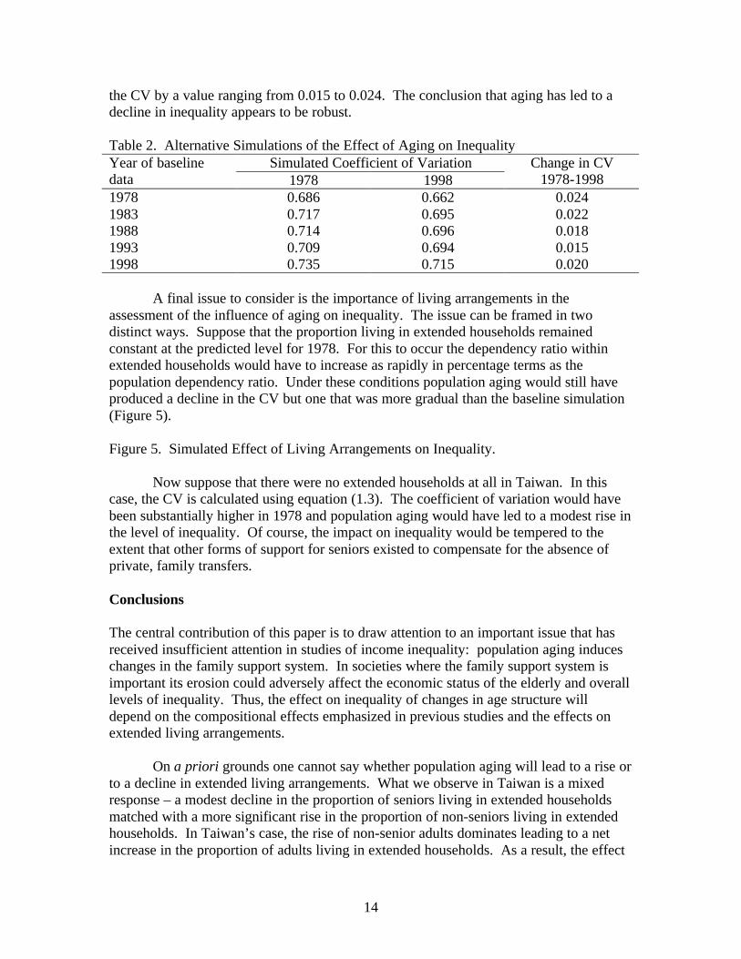
the CV by a value ranging from 0.015 to 0.024. The conclusion that aging has led to a decline in inequality appears to be robust. Table 2. Alternative Simulations of the Effect of Aging on Inequality
Simulated Coefficient of Variation Year of baseline data 1978 1998
Change in CV 1978-1998
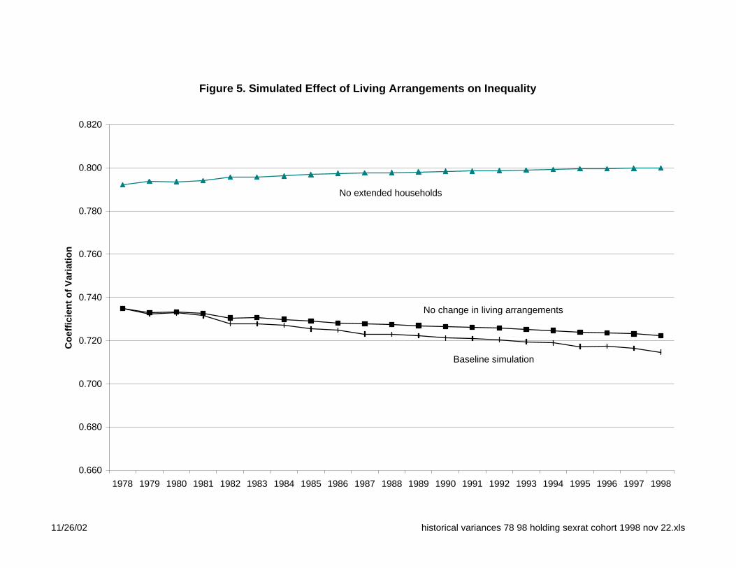
1978 0.686 0.662 0.024 1983 0.717 0.695 0.022 1988 0.714 0.696 0.018 1993 0.709 0.694 0.015 1998 0.735 0.715 0.020 A final issue to consider is the importance of living arrangements in the assessment of the influence of aging on inequality. The issue can be framed in two distinct ways. Suppose that the proportion living in extended households remained constant at the predicted level for 1978. For this to occur the dependency ratio within extended households would have to increase as rapidly in percentage terms as the population dependency ratio. Under these conditions population aging would still have produced a decline in the CV but one that was more gradual than the baseline simulation (Figure 5). Figure 5. Simulated Effect of Living Arrangements on Inequality. Now suppose that there were no extended households at all in Taiwan. In this case, the CV is calculated using equation (1.3). The coefficient of variation would have been substantially higher in 1978 and population aging would have led to a modest rise in the level of inequality. Of course, the impact on inequality would be tempered to the extent that other forms of support for seniors existed to compensate for the absence of private, family transfers. Conclusions The central contribution of this paper is to draw attention to an important issue that has received insufficient attention in studies of income inequality: population aging induces changes in the family support system. In societies where the family support system is important its erosion could adversely affect the economic status of the elderly and overall levels of inequality. Thus, the effect on inequality of changes in age structure will depend on the compositional effects emphasized in previous studies and the effects on extended living arrangements. On a priori grounds one cannot say whether population aging will lead to a rise or to a decline in extended living arrangements. What we observe in Taiwan is a mixed response – a modest decline in the proportion of seniors living in extended households matched with a more significant rise in the proportion of non-seniors living in extended households. In Taiwan’s case, the rise of non-senior adults dominates leading to a net increase in the proportion of adults living in extended households. As a result, the effect
15
of aging has been a small, gradual reduction in per capita income inequality between 1978 and 1998. Although the emphasis in this paper is on the effects of aging, this is not the only factor that is influencing income inequality in Taiwan. Our analysis of living arrangements finds a gradual secular decline in the proportion of seniors living in extended households. If this trend continues or accelerates per capita income inequality will rise in Taiwan. If extended households were to disappear altogether the coefficient of variation would rise by 12% given the population age structure that prevailed in 1998. This provides direct quantification of the importance of the family support system in Taiwan. Changes in the distribution of income within the broad age groups we are analyzing and changes in the differences in the mean incomes of seniors and non-seniors are also influencing the overall level of income inequality in Taiwan. These changes are not analyzed directly, but they are responsible for the difference between the actual trend in the coefficient of variation and the effect of aging. These other factors, then, are responsible for a gradual increase in inequality, which has been offset by the effects of aging except for the last few years for which data are available. Other countries in East and Southeast Asia are experiencing demographic change that is every bit as rapid as that experienced by Taiwan. Moreover, the family support system is also important in these countries. Prominent examples are Japan, South Korea, Singapore, Thailand, and China. Their family support systems are subject to the same demographic pressures as Taiwan’s. How those support systems will evolve in response to that pressure and how levels of inequality will be affected are questions that can only be answered by additional research. References Chu, C. Y. C. and L. Jiang (1997). “Demographic Transition, Family Structure, and
Income Inequality.” Review of Economics and Statistics 79(4): 665-69. Deaton, A. S. and C. H. Paxson (1997). “The Effects of Economic and Population
Growth on National Saving and Inequality.” Demography 34(1): 97-114. Lam, D. (1997). Demographic Variables and Income Inequality. Handbook of population
and family economics. Volume 1B. Handbooks in Economics, vol. 14. -. M.-R. Rosenzweig and -. O. Stark, eds,. Amsterdam; New York and Oxford, Elsevier Science: ages 1015-59.
Lee, S.-H. and A. Mason (2002). Aging, Family Transfers, and Income Inequality. 3d Workshop on Demographic Macroeconomic Modeling, Max Planck Institute for Demographic Research, Rostock, Germany.
Liu, P. K. C. (1978). “Demographic Factors in Size-Distribution of Income in Taiwan.” Academia Economic Papers 6(2): 131-156.
Mason, A. and S.-H. Lee (2002). Population Aging and the Extended Family in Taiwan: A New Model for Analyzing and Projecting Living Arrangements. Workshop on
16
Future Seniors and their Kin in honor of Gene Hammel, Marconi Conference Center, Marshall, CA.
Schultz, T. P. (1997). Income Inequality in Taiwan 1976-1995: Changing Family Composition, Aging, and Female Labor Force Participation, Yale U.
White, H. J. (1980). “A Heteroscedasticity-Consistent Covariance Matrix Estimator and Direct Test for Heteroscedasticity.” Econometrica 48: 817-838.
Figure 1 Proportion nuclear and the relative dependency structure by age and birth cohort