J. Fluid Mech. (2012), vol. 710, pp. 379–418. c Cambridge University Press 2012 379 doi:10.1017/jfm.2012.370 On the steady-state fully resonant progressive waves in water of finite depth Dali Xu 2 , Zhiliang Lin 2 , Shijun Liao 1,2 † and Michael Stiassnie 3 1 State Key Laboratory of Ocean Engineering, Shanghai Jiao Tong University, Shanghai 200240, China 2 School of Naval Architecture, Ocean and Civil Engineering, Shanghai Jiao Tong University, Shanghai 200240, China 3 Faculty of Civil and Environmental Engineering, Technion IIT, Haifa 32000, Israel (Received 14 January 2012; revised 30 June 2012; accepted 17 July 2012; first published online 7 September 2012) The steady-state fully resonant wave system, consisting of two progressive primary waves in finite water depth and all components due to nonlinear interaction, is investigated in detail by means of analytically solving the fully nonlinear wave equations as a nonlinear boundary-value problem. It is found that multiple steady- state fully resonant waves exist in some cases which have no exchange of wave energy at all, so that the energy spectrum is time-independent. Further, the steady-state resonant wave component may contain only a small proportion of the wave energy. However, even in these cases, there usually exist time-dependent periodic exchanges of wave energy around the time-independent energy spectrum corresponding to such a steady-state fully resonant wave, since it is hard to be exactly in such a balanced state in practice. This view serves to deepen and enrich our understanding of the resonance of gravity waves. Key words: surface gravity waves 1. Introduction In physics, resonance is the tendency of a system to oscillate at a greater amplitude at some frequencies, i.e. the system’s resonance frequencies, than at others. At these frequencies, even small periodic driving forces can often produce large-amplitude oscillations, because the system stores vibrational energy. The so-called gravity wave resonance has been a hot topic in fluid mechanics since the last century. In his pioneering work, Phillips (1960, 1981) found the resonance criterion of a quartet of progressive waves in deep water, k 1 ± k 2 ± k 3 ± k 4 = 0, ω 1 ± ω 2 ± ω 3 ± ω 4 = 0, (1.1) where k i denotes the wavenumber, ω i = √ gk i with k i =|k i | is the angular frequency, g is the acceleration due to gravity, respectively. In particular, when two of the four waves have the same wavenumber, say, k 1 = k 4 , so that k 3 = 2k 1 - k 2 , ω 3 = 2ω 1 - ω 2 , (1.2) † Email address for correspondence: [email protected]
On the steady-state fully resonant progressivewaves in water of finite depth
Dali Xu2, Zhiliang Lin2, Shijun Liao1,2† and Michael Stiassnie3
1 State Key Laboratory of Ocean Engineering, Shanghai Jiao Tong University, Shanghai 200240, China2 School of Naval Architecture, Ocean and Civil Engineering, Shanghai Jiao Tong University,
Shanghai 200240, China3 Faculty of Civil and Environmental Engineering, Technion IIT, Haifa 32000, Israel
(Received 14 January 2012; revised 30 June 2012; accepted 17 July 2012;first published online 7 September 2012)
The steady-state fully resonant wave system, consisting of two progressive primarywaves in finite water depth and all components due to nonlinear interaction, isinvestigated in detail by means of analytically solving the fully nonlinear waveequations as a nonlinear boundary-value problem. It is found that multiple steady-state fully resonant waves exist in some cases which have no exchange of waveenergy at all, so that the energy spectrum is time-independent. Further, the steady-stateresonant wave component may contain only a small proportion of the wave energy.However, even in these cases, there usually exist time-dependent periodic exchangesof wave energy around the time-independent energy spectrum corresponding to such asteady-state fully resonant wave, since it is hard to be exactly in such a balanced statein practice. This view serves to deepen and enrich our understanding of the resonanceof gravity waves.
Key words: surface gravity waves
1. IntroductionIn physics, resonance is the tendency of a system to oscillate at a greater amplitude
at some frequencies, i.e. the system’s resonance frequencies, than at others. At thesefrequencies, even small periodic driving forces can often produce large-amplitudeoscillations, because the system stores vibrational energy.
The so-called gravity wave resonance has been a hot topic in fluid mechanics sincethe last century. In his pioneering work, Phillips (1960, 1981) found the resonancecriterion of a quartet of progressive waves in deep water,
where ki denotes the wavenumber, ωi = √gki with ki = |ki| is the angular frequency,g is the acceleration due to gravity, respectively. In particular, when two of the fourwaves have the same wavenumber, say, k1 = k4, so that
which comes from the dispersion relation ω23 = gk3 given by the linear wave theory.
In this special case, Phillips (1960) found that the amplitude of the resonant wavecomponent, if it is zero initially, grows linearly with time. This conclusion forsmall times was verified later by Longuet-Higgins (1962) using perturbation methods.Meanwhile, in order to find the physical mechanism of wave resonance, Benney (1962)established the evolution equations of wave mode amplitudes, and demonstrated thewell-known time-dependent periodic exchange of wave energy governed by Jacobianelliptic functions, when Phillips’ resonance criterion is fully or nearly satisfied.Following Benney’s excellent work, Bretherton (1964) solved the evolution equationsof the oscillation amplitudes over a characteristic time.
To check the theoretical results some experiments were done. Longuet-Higgins &Smith (1966) and McGoldrick et al. (1966) experimentally studied the interaction oftwo mutually orthogonal primary wave trains generated in a wave tank, and identifiedthe resonant wave whose amplitude grows with the interaction distance. It was foundthat the resonant wave does not appear when Phillips’ resonant condition is notsatisfied. This experiment demonstrated wave resonance for the first time.
The above-mentioned studies were on resonant waves in deep water. In the shallowwater case, Phillips (1960) pointed out that any pair of parallel gravity waves wouldinteract resonantly with each other, because they have no dispersive property. Recently,based on the quadratic Boussinesq equations, Onorato et al. (2009) studied the energytransfer of shallow water waves, and found that the four-wave resonant interactionsare included naturally. Katsardi & Swan (2011) studied numerically the evolutionof waves propagating unidirectionally in intermediate and shallow water, and foundthat the third-order resonant term is the dominant influence as the water depthreduces.
Following the pioneering work of Phillips (1960), most researchers have focusedon the evolution of resonant waves whose amplitude is zero at t = 0. Obviously,Phillips’ result for a linearly growing resonant wave amplitude is valid only forshort times, otherwise the resonant wave would contain all the wave energy, whichis, however, physically impossible. Physically speaking, if the viscosity of the fluidis neglected, the wave system should be in some kind of stable balanced state ifthe time is sufficiently long. As discovered by Benney (1962), one such balancedstate corresponds to the time-dependent periodic exchange of wave energy betweendifferent wave components. Does there exist some form of balanced state for whichthere is no exchange of wave energy at all when Phillips’ resonance criterion is fullysatisfied?
Liao (2011) investigated this kind of steady state for the nonlinear interaction oftwo trains of propagating waves in deep water. Here, the steady state means that thereis no exchange at all of wave energy between different wave components, that is, allamplitudes of wave components are independent of time. By means of the so-calledhomotopy analysis method (HAM) developed by Liao (1992, 1999, 2003, 2010, 2012),a powerful analytic method for highly nonlinear problems, the exact nonlinear waveequations were solved and the convergent series solutions were obtained in bothresonant and non-resonant cases. Liao (2011) found, for the first time, that this kindof steady-state wave system has three different solutions when Phillips’ resonancecriterion is satisfied! In particular, it is found that, although the amplitude of theresonant wave component is of the same order as that of the two primary waves,
On the steady-state fully resonant progressive waves in water of finite depth 381
it is not always the largest one. In some cases, the amplitude of the resonant wavecomponent is much smaller than the primary ones, i.e. the resonant wave componentscan contain only a small proportion of the total wave energy.
In this article, in order to confirm the above conclusions of Liao (2011) in generalcases, we further investigate this kind of steady-state system for the nonlinearinteraction of two trains of waves propagating in water of finite depth, whenPhillips’ resonance condition is exactly satisfied. This steady-state wave system, ifit does indeed exist, has steady wavenumber, frequency and amplitude for each wavecomponent, which are independent of time. Using the HAM in a similar way, weobtain six different steady-state resonant waves, three more than those given by Liao(2011). Further, it is found once again that the amplitude of the resonant component isnot always dominant: it can be much smaller than that of the primary ones in somecases. This confirms that Liao’s conclusions (2011) concerning steady-state resonantwaves in deep water also hold for steady-state resonant waves in finite water depthand thus have general application. Furthermore, the effect of the water depth onsteady-state resonant waves is investigated for the first time. All of this will help todeepen and enrich our understanding of the resonance for gravity waves.
This paper is organized as follows. The mathematical description of the physicalproblem is given in § 2. The basic idea of the solution procedure in the HAM contextis described in § 3. The multiple solutions of the steady-state resonant waves fora particular case are given in § 4. The multiple solutions of steady-state resonantwaves for some other cases are presented in § 5. Concluding remarks and discussionsfollow in § 6. The detailed mathematical formulas related to the HAM are given inappendix A. Our main conclusions are confirmed by means of Zakharov’s equation, asdescribed briefly in appendix B.
2. The mathematical description2.1. The original initial/boundary-value problem
Let us consider the nonlinear interactions of two trains of progressive gravity waveswith small amplitudes, propagating in water of finite depth d. We assume that thefluid is inviscid and incompressible, the flow is irrotational, and the surface tensionis neglected. The coordinate system (x, y, z) is set on the free surface, with z-axispositive vertically from the free surface. The governing equation of the velocitypotential φ(x, y, z, t) is given by
∇2φ = 0, −d < z< η(x, y, t), (2.1)
subject to the two boundary conditions on the unknown free surface z= η(x, y, t),
∂2φ
∂t2+ g
∂φ
∂z+ ∂ |∇φ|
2
∂t+∇φ ·∇
(12|∇φ|2
)= 0, (2.2)
gη + ∂φ∂t+ 1
2|∇φ|2 = 0, (2.3)
and the bottom boundary condition
∂φ
∂z= 0 at z=−d, (2.4)
382 D. Xu, Z. Lin, S. Liao and M. Stiassnie
where
∇ = i∂
∂x+ j
∂
∂y+ k
∂
∂z(2.5)
is a linear operator, with i, j, k denoting unit vectors in the x, y, z directions,respectively. Here all variables are dimensional.
2.2. Solution formulasAlthough the governing equation (2.1) and the bottom boundary condition (2.4) arelinear, the two nonlinear boundary conditions (2.2) and (2.3) are satisfied on theunknown free surface η(x, y, t). Such nonlinear partial differential equations (PDEs)are difficult to solve in general, often with rather complicated solutions. However,when the so-called steady-state wave system with time-independent wavenumber,frequency and amplitude for each component does indeed exist, the correspondingvelocity potential φ(x, y, z, t) and the wave elevation η(x, y, t) have rather simpleexpressions, as shown below. Our goal is to discover such steady-state resonant waveswhen they do indeed exist.
By means of perturbation methods, Benney (1962) and Bretherton (1964) assumedthat, when there are l primary waves, the wave elevation has the form
where i = √−1, τ = εt, A−l(τ ) is the complex conjugate of Al(τ ), ε is a smallparameter that makes Al(τ ) a slowly varying function, kl is the wavenumber of the lthprimary wave and ω2
l = g|kl| corresponds to the classical linear theory, and r= xi + yjis a spatial vector for (x, y), respectively. Similar expressions can also be found in themonograph by Craik (1988). Benney (1962) and Bretherton (1964) gave the evolutionequations of Al(τ ) and found that Al(τ ) can be expressed in terms of elliptic functions.
Assume that steady-state resonant waves exist, so that the corresponding waveelevation can be expressed by
η(x, y, t)=+∞∑l=1
Al cos(kl · r− σlt), (2.7)
where Al is a constant and σl is the actual frequency. Note that, due to weaklynonlinear effects, the actual frequencies of waves, σ1 and σ2, are often slightlydifferent from the linear dispersion relation ωl = √gkl tanh(kld) and also depend onthe wave amplitudes. The above formula provides the solution for the wave elevation.
Note that the existence of steady-state resonant waves is merely assumed here. Ourstrategy is first to make this assumption and then to prove that the correspondingsteady-state resonant waves do indeed exist in some cases, if they satisfy the fullynonlinear wave equation (2.1)–(2.4). If no such steady-state solutions can be found,it indicates that the assumption is wrong, that is, no steady-state resonant waves canexist. In this way, we can investigate the existence of steady-state resonant waves indetail.
For simplicity, let us consider a steady-state resonant wave system consisting of twoprimary progressive waves with wavenumbers k1 and k2. According to the elevationexpression (2.7), we define the two variables
ξ1 = k1 · r− σ1t, ξ2 = k2 · r− σ2t, (2.8)
On the steady-state fully resonant progressive waves in water of finite depth 383
related to the two primary waves, with the definitions
where kl = |kl| and αl (l = 1, 2) is the angle between the x-axis and the wavenumbervector kl, σl is the wave angular frequency of the lth primary wave, respectively. Usingthe new variables ξ1, ξ2 and the solution expression (2.7), the wave elevation η(x, y, t)of a steady-state resonant wave system is expressed by
η(ξ1, ξ2)=+∞∑m=0
+∞∑n=−∞
am,n cos(mξ1 + nξ2), (2.12)
where am,n is a constant to be determined later. Note that the time t does not appear inthe above expression. Accordingly, the velocity potential φ is dependent only upon ξ1,ξ2 and z. Then, using the above definitions, the governing equation (2.1) becomes
k21
∂2φ
∂ξ 21
+ 2k1 · k2∂2φ
∂ξ1∂ξ2+ k2
2
∂2φ
∂ξ 22
+ ∂2φ
∂z2= 0, −d < z< η(ξ1, ξ2), (2.13)
subject to the boundary conditions on the unknown free surface z= η(ξ1, ξ2),
σ 21
∂2φ
∂ξ 21
+ 2σ1σ2∂2φ
∂ξ1∂ξ2+ σ 2
2
∂2φ
∂ξ 22
+ g∂φ
∂z− 2
(σ1∂f
∂ξ1+ σ2
∂f
∂ξ2
)+ ∇φ · ∇f = 0, (2.14)
η = 1g
(σ1∂φ
∂ξ1+ σ2
∂φ
∂ξ2− f
), (2.15)
and the bottom condition
∂φ
∂z= 0 at z=−d, (2.16)
where
∇ = k1∂
∂ξ1+ k2
∂
∂ξ2+ k
∂
∂z, (2.17)
and
f = 12
[k2
1
(∂φ
∂ξ1
)2
+ 2k1 · k2∂φ
∂ξ1
∂φ
∂ξ2+ k2
2
(∂φ
∂ξ2
)2
+(∂φ
∂z
)2]. (2.18)
Note that the time t disappears in all the above equations. In this way, the originalinitial/boundary-value problem (2.1)–(2.4) becomes a nonlinear boundary-value one,mainly because we are only interested in the steady-state resonant waves butcompletely neglect the corresponding initial conditions for them.
According to the linear governing equation (2.13) and the bottom boundarycondition (2.16), the velocity potential φ(ξ1, ξ2, z) should be in the form
φ(ξ1, ξ2, z)=+∞∑m=0
+∞∑n=−∞
bm,nΨm,n(ξ1, ξ2, z) (2.19)
384 D. Xu, Z. Lin, S. Liao and M. Stiassnie
with the definition
Ψm,n = sin(mξ1 + nξ2)cosh[|mk1 + nk2|(z+ d)]
cosh[|mk1 + nk2|d] , (2.20)
where bm,n is a constant to be determined. Note that (2.19) automatically satisfies thelinear governing equation (2.13) and the bottom boundary condition (2.16). From amathematical viewpoint, our aim is to find the velocity potential φ(ξ1, ξ2, z) and theelevation η(ξ1, ξ2) in the form of (2.12) and (2.19), respectively, which satisfy the twononlinear boundary conditions (2.14) and (2.15) on the free surface z= η(ξ1, ξ2).
3. Analytic approach based on the homotopy analysis methodIn this section, the nonlinear boundary-value problem governed by the PDEs
(2.13)–(2.16) is solved by means of the homotopy analysis method.Traditionally, perturbation methods have been widely applied to solve nonlinear
problems related to gravity waves. It is well known that perturbation methods arestrongly dependent upon small physical parameters, i.e. the so-called perturbationquantities. To overcome the restrictions of perturbation methods and some traditionalnon-perturbation techniques, Liao (1992, 1999, 2003, 2010, 2012) developed ananalytic technique for highly nonlinear problems, namely the homotopy analysismethod (HAM). Unlike perturbation techniques, the HAM is entirely independent ofsmall physical parameters. Further, being based on the homotopy concept in topology,the HAM gives us great freedom in the choice of the initial guess, the equation typeof linear subproblems and the basis functions of solution. In particular, unlike all otheranalytic techniques, the HAM provides a simple way to guarantee the convergenceof approximations and is thus valid for highly nonlinear problems in general. Forexample, unlike asymptotic/perturbation formulas, which are often valid only a coupleof days or weeks prior to expiry, the optimal exercise boundary of an American putoption given by Liao (2012) (see chapter 13) using the HAM may be valid for acouple of dozen years or even half a century. For details on the HAM, refer to the twobooks by Liao (2003, 2012).
3.1. Continuous variationLet φ0(ξ1, ξ2, z), η0(ξ1, ξ2) denote the initial guesses of the steady-state velocitypotential φ(ξ1, ξ2, z) and wave elevation η(ξ1, ξ2), respectively. For simplicity, wechoose η0(ξ1, ξ2) = 0. Let q ∈ [0, 1] denote an embedding parameter and letc0 6= 0 be the so-called convergence-control parameter. Here, both q and c0 areauxiliary parameters without physical meaning. Instead of solving the nonlinear PDEs(2.13)–(2.16) directly, we first construct a family (with respect to q) of PDEs abouttwo continuous variations φ(ξ1, ξ2, z; q) and η(ξ1, ξ2; q), governed by the so-calledzeroth-order deformation equations,
∇2φ(ξ1, ξ2, z; q)= 0, −d < z< η(ξ1, ξ2; q), (3.1)
subject to the two boundary conditions on the unknown free surface z= η(ξ1, ξ2; q),(1− q)L [φ(ξ1, ξ2, z; q)− φ0(ξ1, ξ2, z)] = qc0N1[φ(ξ1, ξ2, z; q)], (3.2)
Thus, as the embedding parameter q ∈ [0, 1] increases from 0 to 1, φ(ξ1, ξ2, z; q)and η(ξ1, ξ2; q) vary continuously from their initial guess solutions φ0(ξ21, ξ2, z)and η0(ξ1, ξ2) = 0 to the exact velocity potential φ(ξ1, ξ2, z) and the wave elevationη(ξ1, ξ2), respectively. Thus, the zeroth-order deformation equations (3.1)–(3.4) indeedconstruct two continuous variations φ(ξ1, ξ2, z; q) and η(ξ1, ξ2; q). Such continuousvariations (or deformations) are called homotopies in topology, expressed by
It should be emphasized that the above two continuous deformations are alsodependent upon the convergence-control parameter c0, which has no physical meaningbut provides a convenient way to guarantee the convergence of approximations,as shown later. In fact, it is the so-called convergence-control parameter c0 thatdifferentiates the HAM from all other analytic techniques, as pointed out by Liao(2012).
The Maclaurin series of φ(ξ1, ξ2, z; q) and η(ξ1, ξ2; q), with respect to theembedding parameter q ∈ [0, 1], reads
φ(ξ1, ξ2, z; q)=+∞∑n=0
φn(ξ1, ξ2, z)qn, (3.14)
η(ξ1, ξ2; q)=+∞∑n=0
ηn(ξ1, ξ2)qn, (3.15)
386 D. Xu, Z. Lin, S. Liao and M. Stiassnie
where
φn(ξ1, ξ2, z)= 1n!∂nφ(ξ1, ξ2, z; q)
∂qn
∣∣∣∣∣q=0
, (3.16)
ηn(ξ1, ξ2)= 1n!∂nη(ξ1, ξ2; q)
∂qn
∣∣∣∣q=0
. (3.17)
Using (3.10) and (3.11) and assuming that the convergence-control parameter c0 isproperly chosen so that the Maclaurin series (3.14) and (3.15) are convergent at q= 1,we have the so-called homotopy-series solution
φ(ξ1, ξ2, z)= φ0(ξ1, ξ2, z)++∞∑n=1
φn(ξ1, ξ2, z), (3.18)
η(ξ1, ξ2)=+∞∑n=1
ηn(ξ1, ξ2). (3.19)
As shown later in § 3.2, the unknown term φn(ξ1, ξ2, z) is governed by a linear PDE,and it is straightforward to obtain ηn(ξ1, ξ2) as long as φn−1(ξ1, ξ2, z) is known. In thisway, the original nonlinear PDEs (2.13)–(2.16) are transformed into an infinite numberof linear PDEs. However, unlike perturbation techniques, such transformation in thecontext of the HAM does not need any small physical parameters. Further, being basedon the concept of homotopy in topology, it gives us great freedom in the choiceof auxiliary linear operator L , the convergence-control parameter c0 and the initialguess φ0(ξ1, ξ2, z), which greatly simplifies resolution of the nonlinear PDEs, as shownbelow.
Since the HAM provides freedom in the choice of auxiliary linear operator, andconsidering the linear part of (2.14), we choose
L φ =(ω2
1
∂2φ
∂ξ 21
+ 2ω1ω2∂2φ
∂ξ1∂ξ2+ ω2
2
∂2φ
∂ξ 22
+ g∂φ
∂z
), (3.20)
where
ω1 =√
gk1 tanh(k1d), ω2 =√
gk2 tanh(k2d) (3.21)
are given by linear wave theory. The above auxiliary linear operator has the property
can be regarded as an eigenvalue of L . Thus, Ψm,n defined by (2.20) can also beregarded as a corresponding eigenfunction of the auxiliary linear operator L .
3.2. High-order deformation equationDifferentiating the zeroth-order deformation equations (3.1)–(3.4) m times with respectto q, then dividing them by m! and setting q = 0, we have the mth-order deformationequation
∇2φm = 0, −d < z< 0, (3.24)
On the steady-state fully resonant progressive waves in water of finite depth 387
subject to the two boundary conditions at z= 0,
L [φm] = c0∆φ
m−1(ξ1, ξ2)− Sm(ξ1, ξ2)+ χmSm−1(ξ1, ξ2), (3.25)
ηm = c0∆η
m−1(ξ1, ξ2)+ χmηm−1, (3.26)
and the bottom condition
∂φm
∂z= 0 z=−d, (3.27)
where
χm =
0 when m 6 1,1 when m> 1.
(3.28)
The detailed expressions of ∆φ
m−1(ξ1, ξ2), Sm(ξ1, ξ2), Sm−1(ξ1, ξ2) and ∆η
m−1(ξ1, ξ2) aregiven in appendix A, and the linear operator L is defined by
L [φm]=(ω2
1
∂2φm
∂ξ 21
+ 2ω1ω2∂2φm
∂ξ1∂ξ2+ ω2
2
∂2φm
∂ξ 22
+ g∂φm
∂z
)∣∣∣∣z=0
, (3.29)
with the property
L −1[sin(mξ1 + nξ2)] = Ψm,n
λm,n, λm,n 6= 0. (3.30)
For details, refer to Liao (2011, 2012). Note that the right-hand sides of (3.25) and(3.26) are only related to approximations at lower orders and are thus regarded asknown. So, it is straightforward to obtain ηm by means of (3.26). Further, Ψm,n
defined by (2.20) automatically satisfies the Laplace equation (3.24) and the boundarycondition (3.27) at bottom. So,
φ∗m = L −1[c0∆
φ
m−1(ξ1, ξ2)− Sm(ξ1, ξ2)+ χmSm−1(ξ1, ξ2)]
(3.31)
gives a special solution of φm. Thus, by means of the inverse operator (3.30) anda computer algebra system such as Mathematica, it is easy to solve the high-orderdeformation equation (3.24) with the linear boundary conditions (3.25)–(3.27).
3.3. Initial guess of potential functionAs mentioned by Chen (1990), Phillips’ resonance criterion of four small-amplitudewaves in water of finite depth, when two of them are equal, reads
where ω1 and ω2 are defined by (3.21). It is interesting that, according to (3.23),we have λ2,−1 = 0 when the above resonance criterion (3.32) is satisfied. Further,according to (3.23), we always have λ1,0 ≡ 0 and λ0,1 ≡ 0, no matter whether theresonance criterion (3.32) is satisfied. In other words, there are three zero eigenvaluesλ1,0, λ0,1 and λ2,−1 when Phillips’ resonance criterion (3.32) is satisfied. Thus, from amathematical viewpoint, the common solution of φm reads
φm = φ∗m + AmΨ1,0 + BmΨ0,1 + CmΨ2,−1, (3.33)
where φ∗m given by (3.31) is a special solution of the mth-order deformation equations(3.24)–(3.27), and Am,Bm,Cm are constants to be determined.
388 D. Xu, Z. Lin, S. Liao and M. Stiassnie
Obviously, according to (3.30), the solution of the high-order deformation equations(3.24)–(3.27) has secular terms when the right-hand side of (3.25) contains the termssin ξ1, sin ξ2 and sin(2ξ1 − ξ2). This is exactly the mathematical reason why the waveamplitude of a resonant wave given by perturbation methods grows linearly with time.Fortunately, the HAM gives us great freedom in the choice of the initial guess solutionφ0(ξ1, ξ2, z), so we can choose the initial guess
φ0(ξ1, ξ1, z)= A0Ψ1,0 + B0Ψ0,1 + C0Ψ2,−1, (3.34)
where A0, B0 and C0 are unknown constants, which are determined by avoiding theabove-mentioned secular terms, as shown later. Note that the above initial guess φ0
automatically satisfies the governing equation (2.13) and the bottom condition (2.16)for arbitrary values of A0,B0,C0.
Note that, from the viewpoint of perturbation methods, (3.34) implies that theresonant wave is of the same order as the primary waves. In fact, if the resonantcomponent is neglected in (3.34), it is impossible to obtain steady-state resonantsolutions. This is exactly the mathematical reason why Phillips (1960, 1981) obtainedthe so-called resonant waves with linearly increasing wave amplitude. Fortunately,since the HAM is independent of small/large physical parameters, we need notconsider the orders of different wave components at all.
4. Steady-state resonant waves for α2 = π/36Without loss of generality, let us first consider the following particular case:
σ1
ω1= σ2
ω2= ε, α1 = 0, α2 = π36
. (4.1)
Here, the value of ε is slightly larger than 1, since Phillips’ criterion (3.32) is validonly for small-amplitude waves.
Substituting all of these parameters into Phillips’ criterion (3.32), we have thefollowing nonlinear algebraic equation:
−494
√4[(k1d)
(k2d)
]2
+ 1− 4(k1d)
(k2d)cos(α2 − α1)
× tanh
(k2d)
√4[(k1d)
(k2d)
]2
+ 1− 4(k1d)
(k2d)cos(α2 − α1)
+ 196
5(k1d)
(k2d)tanh(k1d)+ 49
5tanh(k2d)
− 1965
√(k1d)
(k2d)tanh(k1d)
√tanh(k2d)= 0. (4.2)
Without loss of generality, let us first consider the case of ε = 1.0003 and k2d = 3π/5.In this case, (4.2) has three solutions, k1d = 2.06269, 1.69564 and 0.867072,respectively, corresponding to three resonance states with k2/k1 = 0.913835, 1.11165and 2.173797, labelled A, B and C in figure 1. Obviously, for different k2d and ε, theratios of k2/k1 for the corresponding fully resonant waves are different, as listed intable 1. Note that k2/k1 of resonance state A is always less than 1, k2/k1 of resonancestate B is always greater than 1 but less than 2, k2/k1 of resonance state C is always
On the steady-state fully resonant progressive waves in water of finite depth 389
–0.5 0.5 1.5 2.01.0 2.50
0.6
0.4
0.2
–0.2
–0.4
–0.6
0
FIGURE 1. (Colour online) Ratio of k2/k1 for (4.1) with ε = 1.0003 and k2d = 3π/5 for fullyresonant waves.
TABLE 1. Ratios of k2/k1 for the three different resonance states for (4.1) with various k2dwhen Phillips’ resonance criterion (3.32) is exactly satisfied. The values of A, B and C areobtained by means of k2 = π/5 (m−1) and the corresponding values of d.
greater than 2, respectively. Note also that resonance states B and C in table 1 wereneglected by Liao (2011) for steady-state fully resonant waves in deep water.
4.1. Steady-state fully resonant waves for resonance state AWithout loss of generality, we first take k2/k1 = 0.913835 for (4.1) with k2d = 3π/5as an example, corresponding to resonance state A, to illustrate the above-mentionedanalytic approach in detail.
Since Phillips’ resonance criterion (3.32) is fully satisfied, there are three zeroeigenvalues λ1,0, λ0,1 and λ2,−1, as mentioned above. Thus, according to (3.30), thecoefficients of the terms sin ξ1, sin ξ2 and sin(2ξ1 − ξ2) on the right-hand side of (3.25)
390 D. Xu, Z. Lin, S. Liao and M. Stiassnie
A0 B0 C0
Group A1−0.061834 0.043603 −0.0866169−0.061834 −0.043603 0.0866169
TABLE 2. Solutions of the nonlinear algebraic equations (4.4)–(4.6) when k2/k1 =0.913835 (corresponding to resonance state A) for (4.1) with ε = 1.0003 and k2d = 3π/5.The values of A0,B0 and C0 are obtained by means of k2 = π/5 (m−1) and d = 3 (m).
must be zero so as to avoid the secular terms, because they do not satisfy the solutionexpression (2.19). For example, substituting the initial guess (3.34) into the first-orderdeformation equation (3.25), we have
L [φ1] = c01φ
0 − S1
= b1,0 sin ξ1 + b0,1 sin ξ2 + b2,0 sin 2ξ1 + b0,2 sin 2ξ2
where bm,n depends upon the three unknown coefficients A0, B0 and C0 of the initialguess (3.34). According to (3.30), we must enforce b1,0 = 0, b0,1 = 0 and b2,−1 = 0 toavoid secular terms, which gives us a set of three nonlinear algebraic equations:
−0.00391489+ 0.206A20 + 0.307855B2
0 + 0.413579B0C0 + 0.547011C20 = 0, (4.4)
−0.00352853+0.372512A20+0.13869B2
0+0.247221A20C0/B0+0.495605C2
0 = 0, (4.5)
0.16962A20B0−0.0043213C0+0.45485A2
0C0+0.341129B20C0+0.301249C3
0 = 0. (4.6)
This set of nonlinear algebraic equations (4.4)–(4.6) has 12 solutions with realvalues, as listed in table 2. Each of them corresponds to a steady-state fully resonant
On the steady-state fully resonant progressive waves in water of finite depth 391
wave system, as shown later. They can be divided into three groups called A1, A2and A3: each group has the same values of |A0|, |B0| and |C0|. Note that, for asteady-state fully resonant wave system with the wave elevation in the form (2.12),the wave energy spectrum is determined by the square of wave components, i.e. a2
m,n,and is therefore independent of time. Thus, the three initial guesses φ0(ξ1, ξ2, z) inthe same group lead to the same time-independent spectrum of wave energy. Indeed,our computations based on the convergent analytic series indicate that the waves givenby different initial guess φ0(ξ1, ξ2, z) in the same group have the same wave energyspectrum, as shown later. Therefore, it is necessary for us to investigate only one caseof A0, B0 and C0 in each group.
As long as A0, B0 and C0 are determined, the initial guess φ0(ξ1, ξ2, z) is known.Then, substituting this known φ0 into (3.26), we can directly obtain η1(ξ1, ξ2). Notethat from now on the right-hand side of (4.3) does not contain the terms sin ξ1, sin ξ2
and sin(2ξ1 − ξ2). So, using (3.30), it is straightforward to obtain
φ1 = φ∗1 + A1Ψ1,0 + B1Ψ0,1 + C1Ψ2,−1, (4.7)
where A1, B1 and C1 are unknown constant coefficients, and
is a special solution with the definition dm,n = bm,n/λm,n. Here, the eigenvalue λm,n isgiven by (3.23). So, using a computer algebra system such as Mathematica or Maple,it is rather easy to obtain η1 and φ1 in this way.
When m > 2, the unknown coefficients Am−1, Bm−1 and Cm−1 in the common solution(3.33) can be obtained by avoiding the secular terms in a similar way, except thatthey are determined by a set of linear algebraic equations. As long as Am−1, Bm−1 andCm−1 are known, we can obtain ηm(ξ1, ξ2) and φm(ξ1, ξ2, z) in a similar way. All of thiscan be done efficiently by means of Mathematica or Maple. Thus, we can obtain thehigh-order approximations of the velocity potential φ(ξ1, ξ2, z) and the wave elevationη(ξ1, ξ2) efficiently.
It should be emphasized that the so-called convergence-control parameter c0, whichis used to guarantee the convergence of our approximations, is still unknown at thispoint. The optimal value of c0 corresponds to the fastest decrease of the averagedresidual squares εφm and εηm of the two free-surface boundary conditions, defined by
εφm =1
(1+M)2
M∑i=0
M∑j=0
[m∑
n=0
∆φn (i4 ξ1, j4 ξ2)
]2
, (4.9)
εηm =1
(1+M)2
M∑i=0
M∑j=0
[m∑
n=0
∆ηn(i4 ξ1, j4 ξ2)
]2
, (4.10)
respectively, where ∆φn and ∆η
n are given in appendix A, M is the number of thediscrete points, and
4ξ1 =4ξ2 = πM . (4.11)
392 D. Xu, Z. Lin, S. Liao and M. Stiassnie
c0
–4
–6
–8
–10
–120–2.0 –0.5–1.0–1.5
–2
–3
–4
–5
–6
–7
–8
–9
–100–2.0 –0.5–1.0–1.5
(a)
(b)
FIGURE 2. Residual squares of log10εφm and log10ε
ηm versus c0 for (4.1) with ε = 1.0003,
k2/k1 = 0.913835 and k2d = 3π/5 when A0 = −0.061834, B0 = 0.043603 and C0 =−0.0866169 (corresponding to group A1). Solid line, first-order approximation; dashedline, third-order approximation; dotted line, fifth-order approximation; dash-dot-dotted line,seventh-order approximation.
A convergence theorem given by Liao (2003) (Theorem 2.1) guarantees the rationalityof (4.9) and (4.10). In this paper, M = 10 is used. For example, when A0 =−0.061834,B0 = 0.043603 and C0 = −0.0866169, corresponding to group A1, the averagedresidual squares εφm and εηm at different orders of approximation are as shown infigure 2. It is found that the residual squares of two free-surface boundary conditionshave the smallest values around c0 = −0.98. So, we choose the optimal convergence-
On the steady-state fully resonant progressive waves in water of finite depth 393
m0 5 10 15 20
–2
–4
–6
–8
–10
–12
–14
–16
–18
–20
FIGURE 3. Residual squares of log10εφm and log10ε
ηm versus the approximation order m
for (4.1) with ε = 1.0003, k2/k1 = 0.913835 and k2d = 3π/5 when A0 = −0.061834,B0 = 0.043603 and C0 = −0.0866169 (corresponding to group A1) by means of c0 = −0.98.Solid line, log10ε
φm; dashed line, log10ε
ηm.
Order of approx. Amplitude of wave component Residual squaresm |a1,0|/d |a0,1|/d |a2,−1|/d ε
TABLE 3. The mth-order approximation of |a1,0|/d, |a0,1|/d and |a2,−1|/d by means ofc0 = −0.98, together with the corresponding residual square εφm−1 and εηm−1 for (4.1) withε = 1.0003, k2d = 3π/5 and k2/k1 = 0.913835 (corresponding to resonance state A) whenA0 =−0.061834, B0 = 0.043603 and C0 =−0.0866169 (corresponding to group A1).
control parameter c0 = −0.98. Using this optimal value of c0, the two averagedresidual squares decrease rather quickly, as shown in table 3 and figure 3. Notethat, at the 20th order of approximation, the averaged residual squares of the twofree-surface boundary conditions decrease to the level of 10−17 and 10−15, respectively,which indicates, without doubt, the convergence of our approximation. Note also thatthe approximations of the amplitudes a0,1, a1,0, a2,−1 of the two primary waves cos ξ1,cos ξ2 and the resonant wave component cos(2ξ1 − ξ2) converge quickly, as shown intable 3.
Similarly, we obtain the convergent velocity potential and wave elevation forgroup A2 by means of c0 = −1 and for group A3 by means of c0 = −1.15. Thecorresponding wave amplitudes of the primary and resonant wave components are
TABLE 5. Wave energy distribution for different groups of steady-state fully resonant wavesystems for (4.1) when ε = 1.0003, k2d = 3π/5 and k2/k1 = 0.913835 (corresponding toresonance state A).
listed in table 4. The wave energy distributions for the three groups of waves are givenin table 5, where Π0 denotes the sum of wave energy of the two primary and oneresonant wave components, and Π is the total wave energy of the entire wave system,defined by
Π0 = a21,0 + a2
0,1 + a22,−1, Π =
+∞∑m=0
+∞∑n=−∞
a2m,n, (4.12)
respectively.Now we immediately obtain the solutions of the three groups of the steady-state
fully resonant waves for (4.1) with ε = 1.0003 and k2d = 3π/5 for resonance state A.It is found that the two primary and one resonant wave components as a whole contain∼99 % of the wave energy, and thus all other wave components are negligible. Notethat the resonant wave amplitude a2,−1 is of the same order as that of the two primaryones, i.e.
O(a2,−1)= O(a0,1)= O(a1,0), (4.13)
as shown in table 4. This agrees well with the conclusions given by Benney (1962).Note that the steady-state resonant wave in group A1 contains the largest proportion(75.64 %) of the wave energy. However, the resonant wave component does not alwayscontain the largest proportion of the wave energy for a steady-state wave system: forexample, the resonant wave in group A2 contains only 37.93 % of the wave energy,which is a little less than that of one of the primary ones (40.43 %) but greater thanthat of the other (20.38 %). In particular, the resonant wave in group A3 contains thesmallest proportion (8.03 %) of the wave energy, which is much less than those of
On the steady-state fully resonant progressive waves in water of finite depth 395
Proportion of wave energy Sumk2d (Primary wave) (Primary wave) (Resonant wave)
TABLE 6. Wave energy distribution for group A1 for (4.1) with ε = 1.0003 and variousk2d. The corresponding values of k2/k1 are given in resonance state A in table 1.
Proportion of wave energy Sumk2d (Primary wave) (Primary wave) (Resonant wave)
TABLE 7. Wave energy distribution for group A2 for (4.1) with ε = 1.0003 and variousk2d. The corresponding values of k2/k1 are given in resonance state A in table 1.
the two primary ones (37.8 % and 53.54 %), as shown in table 5. Therefore, steady-state resonant waves also exist in finite water depth, and, further, the resonant wavecomponents can contain only a small proportion of the total wave energy. So, theconclusions given by Liao (2011) for steady-state fully resonant waves in deep waterhave general application.
Unlike Liao (2011), we consider in this article the steady-state resonant waves infinite water depth. So, the effect of water depth is studied here in detail. It is foundthat, in resonance state A, there always exist three different groups of steady-statefully resonant waves in different water depths, called group Ai (i = 1, 2, 3). The waveenergy distributions of the two primary and one resonant components of the threegroups in different water depths are shown in figure 4 and tables 6–8. It is found thatthe resonant wave component in group A1 always contains the largest proportion ofthe wave energy, but that of group A3 always contains the smallest ones.
396 D. Xu, Z. Lin, S. Liao and M. Stiassnie
0
20
40
60
80
1.5 2.5 3.5 4.53.02.0 4.0 5.0
1.5 2.5 3.5 4.53.02.0 4.0 5.0
(a)
(b)
(c)
10
15
20
25
30
35
40
50
45
1.5 2.5 3.5 4.53.02.0 4.0 5.0
0
20
10
40
30
60
50
FIGURE 4. (Colour online) Wave energy distribution for (4.1) with ε = 1.0003 and variousk2d for resonance state A in table 1. (a) Group A1, (b) group A2, (c) group A3. Dash-dottedline, a2
TABLE 8. Wave energy distribution for group A3 for (4.1) with ε = 1.0003 and variousk2d. The corresponding values of k2/k1 are given in resonance state A in table 1.
Based on our above-mentioned results, in resonance state A listed in table 1 there doindeed always exist multiple steady-state fully resonant waves in water of finite depth.Moreover, the amplitude of the resonant wave component is of the same order as thoseof the two primary ones, and the two primary and one resonant wave components as awhole contain nearly 99 % of the wave energy. Furthermore, for steady-state resonantwaves in finite water depth, the resonant wave component can contain a much smallerproportion of the wave energy than the primary ones. Note that the same conclusionswere reported by Liao (2011) for steady-state fully resonant waves in deep water. So,in this subsection, we further verify that Liao’s conclusions still hold in finite waterdepth for resonance state A and thus have general application.
4.2. Steady-state fully resonant waves in resonance state BAs shown in table 1, when Phillips’ resonance criterion is exactly satisfied, thereexist three steady-state resonance states for (4.1) with ε = 1.0003 but different k2d:k2/k1 < 1 for resonance state A, 1< k2/k1 < 2 for resonance state B and k2/k1 > 2 forresonance state C. Note that resonance states B and C were neglected by Liao (2011)for steady-state fully resonant waves in deep water. In this subsection, we focus onresonance state B.
Similarly, we first take k2d = 3π/5 as an example of resonance state B. The analyticapproach is exactly the same as that described in § 4.1, and is thus omitted here. Toavoid the secular terms, we have a set of the nonlinear algebra equations
−0.003107+ 0.0859796A20 + 0.245246B2
0 + 0.172718B0C0 + 0.11889C20 = 0, (4.14)
−0.0035285+ 0.1951A20 + 0.13869B2
0 + 0.0673168A20C0/B0 + 0.13566C2
0 = 0, (4.15)
0.1078A20B0 − 0.002713C0 + 0.151046A2
0C0 + 0.21599B20C0 + 0.0519C3
0 = 0, (4.16)
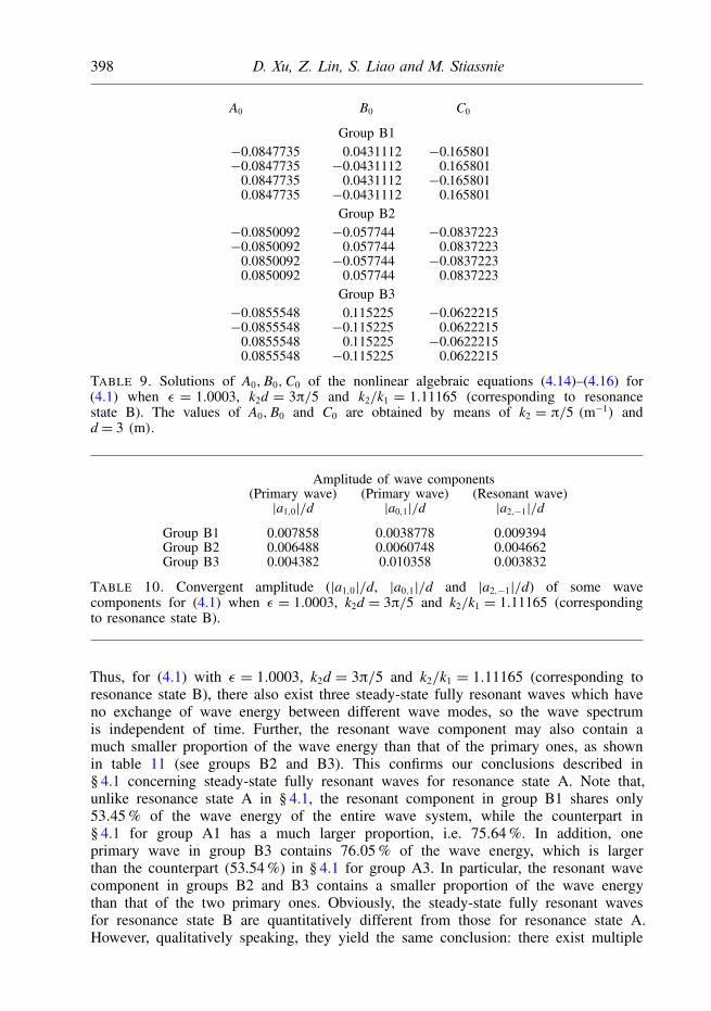
which have 12 solutions with real values. As listed in table 9, they can be divided intothree groups, denoted by groups B1, B2 and B3, respectively, and each group containsfour different solutions but the same values of |A0|, |B0| and |C0|.
Again, choosing an optimal convergent-control parameter c0, we obtain theconvergent analytic approximations for groups B1, B2 and B3, as shown in table 10.
398 D. Xu, Z. Lin, S. Liao and M. Stiassnie
A0 B0 C0
Group B1−0.0847735 0.0431112 −0.165801−0.0847735 −0.0431112 0.165801
TABLE 9. Solutions of A0,B0,C0 of the nonlinear algebraic equations (4.14)–(4.16) for(4.1) when ε = 1.0003, k2d = 3π/5 and k2/k1 = 1.11165 (corresponding to resonancestate B). The values of A0,B0 and C0 are obtained by means of k2 = π/5 (m−1) andd = 3 (m).
TABLE 10. Convergent amplitude (|a1,0|/d, |a0,1|/d and |a2,−1|/d) of some wavecomponents for (4.1) when ε = 1.0003, k2d = 3π/5 and k2/k1 = 1.11165 (correspondingto resonance state B).
Thus, for (4.1) with ε = 1.0003, k2d = 3π/5 and k2/k1 = 1.11165 (corresponding toresonance state B), there also exist three steady-state fully resonant waves which haveno exchange of wave energy between different wave modes, so the wave spectrumis independent of time. Further, the resonant wave component may also contain amuch smaller proportion of the wave energy than that of the primary ones, as shownin table 11 (see groups B2 and B3). This confirms our conclusions described in§ 4.1 concerning steady-state fully resonant waves for resonance state A. Note that,unlike resonance state A in § 4.1, the resonant component in group B1 shares only53.45 % of the wave energy of the entire wave system, while the counterpart in§ 4.1 for group A1 has a much larger proportion, i.e. 75.64 %. In addition, oneprimary wave in group B3 contains 76.05 % of the wave energy, which is largerthan the counterpart (53.54 %) in § 4.1 for group A3. In particular, the resonant wavecomponent in groups B2 and B3 contains a smaller proportion of the wave energythan that of the two primary ones. Obviously, the steady-state fully resonant wavesfor resonance state B are quantitatively different from those for resonance state A.However, qualitatively speaking, they yield the same conclusion: there exist multiple
On the steady-state fully resonant progressive waves in water of finite depth 399
Distribution of wave energy Sum(Primary wave) (Primary wave) (Resonant wave)
TABLE 11. Wave energy distribution of the three steady-state fully resonant waves for (4.1)when ε = 1.0003, k2d = 3π/5 and k2/k1 = 1.11165 (corresponding to resonance state B).
Proportion of wave energy Sumk2d (Primary wave) (Primary wave) (Resonant wave)
TABLE 12. Wave energy distribution for group B1 for (4.1) with ε = 1.0003 and variousk2d. The corresponding values of k2/k1 are given in resonance state B in table 1.
steady-state fully resonant waves whose resonant wave component can contain only asmall proportion of the wave energy.
The wave energy distributions of three steady-state fully resonant waves in differentwater depth d are as shown in figure 5 and in tables 12–14, where group Bi(i = 1, 2, 3) denotes the ith group of steady-state fully resonant waves in variouswater depths for resonance state B. It is found that there always exist three steady-statefully resonant waves, and that the resonant wave component may also contain muchless wave energy than the primary ones. This confirms that our conclusions given in§ 4.1 for resonance state A have general application.
4.3. Steady-state fully resonant waves in resonance state CLet us further consider the steady-state fully resonant waves for (4.1) with ε = 1.0003,k2d = 3π/5 and k2/k1 = 2.173797, corresponding to resonance state C in figure 1.
Similarly, to avoid the secular terms, we have a set of nonlinear algebraic equationsin the three unknown coefficients of the initial guess (3.34):
−0.118972+ 0.252909A20 + 9.45119B2
0 + 0.51183B0C0 − 0.00520192C20 = 0, (4.17)
−0.352853+ 1.19945A20 + 13.869B2
0 + 0.037475A20C0/B0 − 0.039547C2
0 = 0, (4.18)
1.9347A20B0 − 0.009184C0 + 0.05405A2
0C0
+ 0.7807B20C0 − 5.378× 10⁻⁴C3
0 = 0. (4.19)
400 D. Xu, Z. Lin, S. Liao and M. Stiassnie
0
20
10
40
30
60
50
1.5 2.5 3.5 4.53.02.0 4.0 5.0
1.5 2.5 3.5 4.53.02.0 4.0 5.015
20
25
30
35
40
45
1.5 2.5 3.5 4.53.02.0 4.0 5.00
20
40
60
80
(a)
(b)
(c)
FIGURE 5. (Colour online) Wave energy distribution for (4.1) with ε = 1.0003 and variousk2d for resonance state B in table 1. (a) Group B1, (b) group B2, (c) group B3. Dash-dottedline, a2
TABLE 13. Wave energy distribution for group B2 for (4.1) with ε = 1.0003 and variousk2d. The corresponding values of k2/k1 are given in resonance state B in table 1.
Proportion of wave energy Sumk2d (Primary wave) (Primary wave) (Resonant wave)
TABLE 14. Wave energy distribution for group B3 for (4.1) with ε = 1.0003 and variousk2d. The corresponding values of k2/k1 are given in resonance state B in table 1.
The above equations have eight different solutions with real values. They can bedivided into two groups (called groups C1 and C2), each containing four differentsolutions with the same values of |A0|, |B0| and |C0|, as listed in table 15.
However, using the same HAM-based approach, we cannot obtain convergentanalytic approximations by means of these values of A0,B0 and C0 in groups C1and C2, mainly because there does not exist a so-called convergence-control parameterc0 such that the convergence of the approximation series can be guaranteed. This isquite different from resonance states A and B, in which it is easy to find the optimalconvergence-control parameter c0 to obtain convergent approximations, as shown forexample in figures 2 and 3.
Note that the existence of steady-state fully resonant waves is merely assumed, andour strategy is first to make this assumption and then to prove that the correspondingsteady-state fully resonant waves do indeed exist in some cases. If no such steady-state
402 D. Xu, Z. Lin, S. Liao and M. Stiassnie
A0 B0 C0
Group C1−0.586361 −0.0596741 −5.92466−0.586361 0.0596741 5.92466
TABLE 15. Solutions of the nonlinear algebraic equations (4.17)–(4.19) for (4.1) withε = 1.0003, k2d = 3π/5 and k2/k1 = 2.173797, corresponding to resonance state C infigure 1. The values of A0,B0 and C0 are obtained by means of k2 = π/5 (m−1) andd = 3 (m).
solutions can be found, this indicates that the assumption is wrong, that is, no steady-state fully resonant waves can exist. Therefore, steady-state fully resonant waves donot exist for (4.1) with ε = 1.0003, k2d = 3π/5 and k2/k1 = 2.173797, correspondingto resonance state C in figure 1.
In summary, for (4.1) with ε = 1.0003 and k2d = 3π/5, there exist three resonancestates with k2/k1 = 0.913835 (resonance state A), k2/k1 = 1.11165 (resonance state B)and k2/k1 = 2.173797 (resonance state C), respectively, as shown in figure 1 andtable 1. Using the HAM-based analytic approach, it is found that, in resonance statesA and B, there exist multiple steady-state fully resonant waves and, further, theresonant wave component can contain only a small proportion of the wave energy.However, in resonance state C, such steady-state fully resonant waves do not exist.These conclusions hold for various water depths including deep water. Note that usingthe famous Zakharov equation we can obtain the same conclusions qualitatively, asshown in appendix B.
5. Steady-state fully resonant waves with different angles between primarywaves
As mentioned above, when the angle between the two primary waves is π/36,there exist multiple steady-state fully resonant waves and, moreover, the resonant wavecomponent can contain only a small proportion of the wave energy, as shown in § 4.1for resonance state A (k2/k1 < 1) and in § 4.2 for resonance state B (1 < k2/k1 < 2).However, no steady-state fully resonant waves are found for resonance state C, asshown in § 4.3. Here, we further illustrate that the these conclusions still hold for someother angles between the two primary waves, and thus have general application.
Without loss of generality, we still consider the case
σ1
ω1= σ2
ω2= 1.0003, α1 = 0, k2d = 3π/5, (5.1)
as an example. One primary wave propagates in the x direction (i.e. α1 = 0) withunknown magnitude k1, i.e. k1 = k1i. The other has wavenumber k2 with knownmagnitude but unknown angle α2. Without loss of generality, we consider two cases,α2 = π/60 and α2 = 2π/45.
On the steady-state fully resonant progressive waves in water of finite depth 403
Distribution of wave energy Sum(Primary wave) (Primary wave) (Resonant wave)
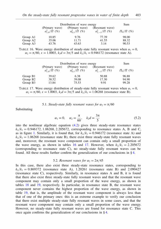
TABLE 16. Wave energy distribution of steady-state fully resonant waves when α1 = 0,α2 = π/60, ε = 1.0003, k2d = 3π/5 and k2/k1 = 0.946172 (resonance state A).
Distribution of wave energy Sum(Primary wave) (Primary wave) (Resonant wave)
TABLE 17. Wave energy distribution of steady-state fully resonant waves when α1 = 0,α2 = π/60, ε = 1.0003, k2d = 3π/5 and k2/k1 = 1.06268 (resonance state B).
5.1. Steady-state fully resonant waves for α2 = π/60
Substituting
α1 = 0, α2 = π60, k2d = 3π
5(5.2)
into the nonlinear algebraic equation (4.2) gives three steady-state resonance statesk2/k1 = 0.946172, 1.06268, 2.205672, corresponding to resonance states A, B and C,as in figure 1. Similarly, it is found that, for k2/k1 = 0.946172 (resonance state A) andk2/k1 = 1.06268 (resonance state B), there exist three steady-state fully resonant wavesand, moreover, the resonant wave component can contain only a small proportion ofthe wave energy, as shown in tables 16 and 17. However, when k2/k1 = 2.205672(corresponding to resonance state C), no steady-state fully resonant waves can befound. All these results further confirm the generalization of our conclusions in § 4.
5.2. Resonant waves for α2 = 2π/45
In this case, there also exist three steady-state resonance states, corresponding tok2/k1 = 0.869372 (resonance state A), 1.20261 (resonance state B) and 2.090427(resonance state C), respectively. Similarly, in resonance states A and B, it is foundthat there also exist three steady-state fully resonant waves and that the resonant wavecomponent may contain only a small proportion of the wave energy, as shown intables 18 and 19, respectively. In particular, in resonance state B, the resonant wavecomponent never contains the highest proportion of the wave energy, as shown intable 19, that is, the amplitude of the resonant wave component is always less thanthat of one of the primary ones: this is an extreme example to verify our conclusionthat there exist multiple steady-state fully resonant waves in some cases, and that theresonant wave component may contain only a small proportion of the wave energy.However, no steady-state fully resonant waves are found for resonance state C. Thisonce again confirms the generalization of our conclusions in § 4.
404 D. Xu, Z. Lin, S. Liao and M. Stiassnie
Distribution of wave energy Sum(Primary wave) (Primary wave) (Resonant wave)
TABLE 18. Wave energy distribution of three steady-state fully resonant waves whenα1 = 0, α2 = 2π/45, ε = 1.0003, and k2d = 3π/5 and k2/k1 = 0.869372 (corresponding toresonance state A).
Distribution of wave energy Sum(Primary wave) (Primary wave) (Resonant wave)
TABLE 19. Wave energy distribution of three steady-state fully resonant waves whenα1 = 0, α2 = 2π/45, ε = 1.0003, k2d = 3π/5 and k2/k1 = 1.20261 (corresponding toresonance state B).
This verifies that our conclusions given in §§ 4.1 and 4.2 have general application.Thus, when Phillips’ resonance criterion (3.32) in finite water depth is exactly satisfied,there may indeed exist, in some cases, multiple steady-state fully resonant waveswhich have no exchange of wave energy, so that the corresponding wave spectrumis independent of time. Moreover, the resonant wave component may contain only asmall proportion of the wave energy in some cases. However, such steady-state fullyresonant waves do not always exist: for example, no steady-state fully resonant wavesare found for resonance state C investigated in this article.
Physically speaking, such steady-state fully resonant progressive waves do exist insome cases, corresponding to a time-independent energy spectrum. However, even inthese cases, there usually exist time-dependent periodic exchanges of wave energygoverned by Jacobian elliptic functions, around the time-independent energy spectrumof a steady-state fully resonant wave, since it is hard to be exactly in such a balancedstate in practice. So, our conclusions reported in this article might deepen and enrichunderstanding of the excellent work of Phillips (1960) and Benney (1962) on waveresonance.
6. Conclusions and discussionPhillips (1960) gave the wave resonance criterion in his pioneering work; it was then
re-derived by Longuet-Higgins (1962) using perturbation methods with the assumptionthat the amplitudes of two primary waves are of the same order but amplitudes ofother wave components are much smaller. Phillips (1960) pointed out that, when theresonance criterion is satisfied, the amplitude of the resonant wave component, if zeroinitially, grows linearly with time t. However, the time t mentioned in Phillips’ aboveconclusion must be small, otherwise the resonant wave component would contain mostof the wave energy and thus break.
On the steady-state fully resonant progressive waves in water of finite depth 405
Benney (1962) established the evolution equations of wave mode amplitudes, anddemonstrated the well-known time-dependent periodic exchange of wave energygoverned by Jacobian elliptic functions, when Phillips’ resonance criterion is fullyor nearly satisfied. Mathematically speaking, the evolution equations of Benney(1962) correspond to a nonlinear initial value problem. Physically speaking, the time-dependent periodic exchange of wave energy leads to a time-dependent periodic energyspectrum.
Liao (2011) first investigated the existence of steady-state fully resonant wavesystems in deep water when Phillips’ resonance criterion is exactly satisfied. Here,the steady-state wave system consists of two progressive primary waves and all otherwave components are due to nonlinear interaction and, further, each wave componenthas time-independent wavenumber, frequency and amplitude. Mathematically speaking,this is a nonlinear boundary-value problem. By means of the homotopy analysismethod (HAM), Liao (2011) found, for the first time, that multiple steady-state fullyresonant waves do indeed exist in deep water in some cases and, moreover, that theresonant wave component may contain only a small proportion of the wave energy.
To check the generalization of Liao’s above-mentioned conclusions for steady-statefully resonant waves in deep water, we further investigate the existence of suchsteady-state fully resonant wave systems in water of finite depth, consisting of twoprogressive primary waves and all other components due to nonlinear interaction.Using the HAM as an analytic tool for the corresponding nonlinear boundary-valueproblem, it is found that such steady-state fully resonant waves in water of finite depthalso exist in some cases, which have no exchange of wave energy between differentwave components and thus a time-independent spectrum of energy, and further thatthe resonant component may contain only a small proportion of the wave energy.The same conclusions are obtained in various water depths by means of differentangles between the two primary waves. It should be emphasized that qualitativelyidentical conclusions are obtained by using the famous Zakharov equation, as shownin appendix B. All of these verify the generalization of our conclusions concerningsteady-state fully resonant waves. Further, it is worth mentioning that Madsen &Fuhrman (2012) numerically solved the harmonic resonance of irregular waves inwater of finite depth, combined with a third-order perturbation approximation. Theirnumerical results, based on a high-order Boussinesq-type formulation, show a boundresonant wave field having constant amplitude in space, consistent with the steady-state fully resonant waves reported in this paper, although they did not find multiplesteady-state resonance waves.
As reported in this article, in some cases (for example, all of resonance state Cinvestigated in this article) steady-state fully resonant waves do not exist, so there onlyexist time-dependent periodic exchanges of wave energy as reported by Benney (1962).However, in some cases, such as resonance states A and B considered in this article,steady-state fully resonant waves do indeed exist with time-independent energy spectra.But even in these cases there usually exist time-dependent periodic exchanges of waveenergy around a time-independent energy spectrum of a corresponding steady-statefully resonant wave, since it is hard to be exactly in such a balanced state in practice.This view might deepen our understanding of wave resonance and enrich the excellentwork of Phillips (1960) and Benney (1962).
Note that Phillips’ resonance criterion can be derived in the context of perturbationtheory by assuming that only amplitudes of two primary waves are of the same orderbut others are at higher order of a small physical parameter. However, using the HAMin this article, we do not need any such assumption: this is an advantage of the
406 D. Xu, Z. Lin, S. Liao and M. Stiassnie
HAM over the perturbation approach. Further, the HAM provides a convenient wayto guarantee the convergence of approximations: this differentiates the HAM from allother analytic techniques. It should be emphasized that the linear governing equationand the bottom boundary conditions are automatically satisfied, and, moreover, theaveraged residual squares of the two boundary conditions on the free surface generallydecrease to the level of 10−15 and 10−17, respectively. So, from a mathematicalviewpoint, we are quite sure that the steady-state fully resonant waves obtained aresolutions of the nonlinear boundary-value problem governed by (2.1)–(2.4). Note thatall steady-state fully resonant waves are obtained by means of the same analyticapproach with the same code. So, if a resonant wave component with maximumamplitude is acceptable, we have identical reasons to believe that the resonant wavecomponent with the smallest amplitude is acceptable too.
Our computations confirm that the resonant wave component is indeed of thesame order as the primary ones. This is consistent with experimental and numericalresults. Note that, in the context of perturbation theory, only the two primary wavesare assumed to be initially of the same order. This assumption of the perturbationapproach is correct only in the case of non-resonance. Restricted by this assumption,perturbation results (usually at the third order of approximation) contain the so-calledsecular terms when Phillips’ criterion is satisfied, so ‘the perturbation theory breaksdown due to singularities in the transfer functions’, as recently pointed out byMadsen & Fuhrman (2012). Unlike the perturbation approach, the HAM is entirelyindependent of any small/large physical parameters: it does not need to make anyassumptions about the amplitudes of wave components. Note that our analytic HAM-based approach successfully avoids the so-called ‘secular terms’ or ‘singularities inthe transfer functions’ of perturbation methods, and provides the multiple solutions ofsteady-state fully resonant waves for the first time. This illustrates the validity andgreat potential of the HAM for complicated nonlinear problems.
Note that two progressive primary waves with small amplitudes are considered inthis paper, mainly because Phillips’ resonance criterion is given for waves with smallwave amplitude. Obviously, it would be very interesting to investigate steady-statefully resonant wave systems consisting of two or more primary waves with largewave amplitudes and all components due to nonlinear interaction. Further, it would bevaluable to investigate steady-state fully resonant waves between two layer flows, or inperiodically variable water depth, or with surface tension, and so on. In addition, thestability of steady-state fully resonant waves should also be investigated in detail.
Acknowledgements
The authors are indebted to Professor C. C. Mei (MIT, USA) for his valuablesuggestions and discussions. We thank the reviewers for their valuable commentsand suggestions. We thank the National Natural Science Foundation (Approval No.10572095) and State Key Lab of Ocean Engineering (Approval No. GKZD010053,GKZD010056) for financial support. This work is also partly supported by the Lloyd’sRegister Educational Trust through the joint centre involving Shanghai Jiao TongUniversity, University College London and Harbin Engineering University. The Lloyd’sRegister Educational Trust is an independent charity working to achieve advances intransportation, science, engineering and technology education, training and researchworldwide for the benefit of all.
On the steady-state fully resonant progressive waves in water of finite depth 407
Appendix A. Definitions of ∆φm,∆
ηm, Sm, Sm and χm in (3.25) and (3.26)
Definitions of ∆φm,∆
ηm, Sm, and Sm in (3.25) and (3.26) are given by
∆φ
m−1 = σ 21 φ
2,0m−1 + 2σ1σ2φ
1,1m−1 + σ 2
2 φ0,2m−1 + gφ0,0
z,m−1
− 2(σ1Γm−1,1 + σ2Γm−1,2
)+Λm−1, (A 1)
∆η
m−1 = ηm−1 − 1g
[(σ1φ
1,0m−1 + σ2φ
0,1m−1)− Γm−1,0
], (A 2)
Sn =n−1∑m=1
(ω2
1βn−m,m2,0 + 2ω1ω2β
n−m,m1,1 + ω2
2βn−m,m0,2 + gγ n−m,m
0,0
), (A 3)
Sn =n−1∑m=0
(ω2
1βn−m,m2,0 + 2ω1ω2β
n−m,m1,1 + ω2
2βn−m,m0,2 + gγ n−m,m
0,0
), (A 4)
where
Γm,0 = k21
2
m∑n=0
φ1,0n φ1,0
m−n + k1 · k2
m∑n=0
φ1,0n φ0,1
m−n
+ k22
2
m∑n=0
φ0,1n φ0,1
m−n +12
m∑n=0
φ0,0z,n φ
0,0z,m−n, (A 5a)
Γm,1 =m∑
n=0
(k2
1φ1,0n φ2,0
m−n + k22φ
0,1n φ1,1
m−n + φ0,0z,n φ
1,0z,m−n
)+ k1 · k2
m∑n=0
(φ1,0
n φ1,1m−n + φ2,0
n φ0,1m−n
), (A 5b)
Γm,2 =m∑
n=0
(k2
1φ1,0n φ1,1
m−n + k22φ
0,1n φ0,2
m−n + φ0,0z,n φ
0,1z,m−n
)+ k1 · k2
m∑n=0
(φ1,0
n φ0,2m−n + φ0,1
n φ1,1m−n
), (A 5c)
Γm,3 =m∑
n=0
(k2
1φ1,0n φ1,0
z,m−n + k22φ
0,1n φ0,1
z,m−n + φ0,0z,n φ
0,0zz,m−n
)+ k1 · k2
m∑n=0
(φ1,0
n φ0,1z,m−n + φ0,1
n φ1,0z,m−n
), (A 5d)
Λm =m∑
n=0
(k2
1φ1,0n Γm−n,1 + k2
2φ0,1n Γm−n,2 + φ0,0
z,nΓm−n,3
)+ k1 · k2
m∑n=0
(φ1,0
n Γm−n,2 + φ0,1n Γm−n,1
), (A 5e)
408 D. Xu, Z. Lin, S. Liao and M. Stiassnie
with the definitions
µ1,n = ηn, n > 1, (A 6)
µm,n =n−1∑
i=m−1
µm−1,iηn−i, m > 2, n > m, (A 7)
ψn,mi, j =
∂ i+j
∂ξ i1∂ξ
j2
(1m!∂mφn
∂zm
∣∣∣∣z=0
), (A 8)
βn,0i, j = ψn,0
i, j , (A 9)
βn,mi, j =
m∑s=1
ψn,si, jµs,m m > 1, (A 10)
γ n,0i, j = ψn,1
i, j , (A 11)
γ n,mi, j =
m∑s=1
(s+ 1)ψn,s+1i, j µs,m m > 1, (A 12)
δn,0i, j = 2ψn,2
i, j , (A 13)
δn,mi, j =
m∑s=1
(s+ 1)(s+ 2)ψn,s+2i, j µs,m m > 1, (A 14)
φi, jn =
n∑m=0
βn−m,mi, j , (A 15)
φi, jz,n =
n∑m=0
γ n−m,mi, j , (A 16)
φi, jzz,n =
n∑m=0
δn−m,mi, j . (A 17)
For details, refer to Liao (2011, 2012).
Appendix B. Steady-state fully resonating quartet given by Zakharov’sequation
A linearly resonating quartet, with wavenumbers kj and frequencies ωj, where kj
and ωj, j = 1, 2, 3, 4, are related by the linear dispersion relation ω2j = gkj tanh(kjd),
satisfies the equations
k1 + k2 = k3 + k4, ω1 + ω2 = ω3 + ω4. (B 1)
Due to weak nonlinear effects, the actual frequencies of the waves, σj, are slightlydifferent from ωj, and also depend on the wave amplitudes. These changes aresometimes called Stokes’ corrections. A fully resonating quartet is defined here asone that satisfies (B 1), as well as
σ1 + σ2 = σ3 + σ4. (B 2)
Here we use Zakharov’s equation to show that the amplitudes of fully resonatingquartets can indeed be time-independent in some cases.
On the steady-state fully resonant progressive waves in water of finite depth 409
Zakharov (1968) assumed that the wave field can be divided into free and boundcomponents. For the special resonant quartet
i = √−1 is the imaginary unit and Ta,b,c,d is the kernel given in chapter 14 inMei, Stiassnie & Yue (2005). Here, we use the formulas of Ta,a,a,a and Ta,b,a,b
derived by Stiassnie & Gramstad (2009). The authors would like to thank Dr OdinGramstad for his correction of the misprint in (4.10) given by Stiassnie & Gramstad(2009) during the private discussion. The expression of T (S)a,a,a,a which we actually usein this paper is T (S)a,a,a,a = −g/(16π2(gd − Cg2
a))4k2a[1 + (Cga/kaωa)(k2
a − (ω4a/g
2))] +(k2
a − (ω4a/g
2))2(gd/ω2
a).Assume that steady-state fully resonant waves exist. We search for the corresponding
solution of Bj(t) in the form
Bj(t)= bje−iΩjt, j= 1, 2, 3, (B 10)
where Ωj = σj − ωj is a real constant, and
bj = |bj|ei arg bj, j= 1, 2, 3, (B 11)
where arg bj denotes the argument of bj.Substituting (B 5) and (B 10) into the wave elevation
η = 12π
∫ ∞−∞
(ω(k)2g
)1/2
B(k, t)ei[k·x−ω(k)t] + ∗ dk (B 12)
gives the steady-state resonant wave elevation
η =3∑
j=1
aj cos(kj · x− σjt + arg bj), (B 13)
where
aj =(ωj
2g
)1/2 |bj|π, j= 1, 2, 3, (B 14)
410 D. Xu, Z. Lin, S. Liao and M. Stiassnie
are constants independent of time. Note that, for the fully resonating special quartet(B 4), we have
2Ω1 −Ω2 =Ω3, (B 15)
and thus
Ωj = (ε − 1)ωj, j= 1, 2, 3; see (4.1). (B 16)
Substituting (B 10) and (B 15) into (B 6)–(B 8), we have the set of nonlinear algebraicequations
where β = 2 arg b1 − arg b2 − arg b3. We must have eiβ = ±1 so that the value of |bj|can be real. Instead of solving the algebraic equations (B 17)–(B 19), we can solve
where x = ±|b1|, y = ±|b2|, z = ±|b3| must be real constants, with the restrictionyz < 0 corresponding to the case of eiβ = −1 and yz > 0 to eiβ = 1, respectively.For (4.1) with ε = 1.0003, k2/k1 = 0.913835 and k2d = 3π/5, corresponding toresonance state A in figure 1, the above nonlinear algebraic equations (B 20)–(B 22)have 12 real solutions of x, y, z. They can be divided into three groups, calledgroups ZA1, ZA2 and ZA3 as listed in table 20, and each group has the samevalues of |x|, |y|, |z|, corresponding to |b1|, |b2|, |b3| in (B 17)–(B 19). Thus, thecorresponding wave elevation (B 13) is steady-state, i.e. each corresponding amplitudeaj is independent of time. This confirms that the steady-state solution expression (2.19)for the HAM-based approach does indeed hold in some cases. Note that any Bj(t) ineach group has a time-independent norm |Bj(t)| and, moreover, |B3(t)| related to theresonant wave component b3 may be the largest, the smallest and in the middle, asshown in figure 6. These results qualitatively agree well with those obtained by theHAM-based approach for the same case.
For (4.1) with ε = 1.0003, k2d = 3π/5 and k2/k1 = 1.11165, corresponding toresonance state B in figure 1, the nonlinear algebraic equations (B 20)–(B 22) alsohave 12 real solutions. They can be divided into three groups, called groups ZB1, ZB2and ZB3 as listed in table 21, respectively. Therefore, the corresponding fully resonantwaves are also steady-state, i.e. aj in (B 13) is independent of time so the solutionexpression (2.19) for the HAM-based approach holds in this case too. Similarly, anyBj(t) in each group has the same time-independent norm |Bj(t)|. It is found that |B3(t)|in group ZB1 is the largest, but |B3(t)| in groups ZB2 and ZB3 are the smallest,as shown in figure 7. These results qualitatively agree well with those given by theHAM-based approach.
On the steady-state fully resonant progressive waves in water of finite depth 411
–0.3
0.3
–0.2
0.2
–0.1
0.1
0
0.3–0.2 0.2–0.1 0.10
(a)
(b)
(c)
–0.3
–0.2
0.2
–0.1
0.1
0
–0.2 0.2–0.1 0.10
–0.3
–0.4
0.4
0.3
–0.2
0.2
–0.1
0.1
0
–0.3–0.4 0.40.3–0.2 0.2–0.1 0.10
FIGURE 6. (Colour online) Time-independent norm |Bj(t)| of (B 6)–(B 8) for (4.1) with ε =1.0003, k2d = 3π/5 and k2/k1 = 0.913835. (a) Group ZA1, (b) group ZA2, (c) group ZA3.Dash-dotted line, B1(t); dashed line, B2(t); solid line, B3(t).
412 D. Xu, Z. Lin, S. Liao and M. Stiassnie
–0.4
–0.6
0.4
0.6
–0.2
0.2
0
0.4 0.60.2–0.4–0.6 –0.2 0
0.40.20–0.4 –0.2
(a)
(b)
(c)
–0.3
0.3
–0.2
0.2
–0.1
0.1
0
0.30.20.1–0.3 –0.2 –0.1 0
0
–0.4
0.4
–0.2
0.2
FIGURE 7. (Colour online) Time-independent norm |Bj(t)| of (B 6)–(B 8) for (4.1) withε = 1.0003, k2d = 3π/5 and k2/k1 = 1.11165. (a) Group ZB1, (b) group ZB2, (c) group ZB3.Dash-dotted line, B1(t); dashed line, B2(t); solid line, B3(t).
On the steady-state fully resonant progressive waves in water of finite depth 413
TABLE 20. Real solutions of (B 20)–(B 22) for (4.1) with ε = 1.0003, k2d = 3π/5 andk2/k1 = 0.913835, corresponding to resonance state A in figure 1. The values of x, y and zare obtained by means of k2 = π/5 (m−1) and d = 3 (m).
TABLE 21. Real solutions of (B 20)–(B 22) for (4.1) with ε = 1.0003, k2d = 3π/5 andk2/k1 = 1.11165, corresponding to resonance state B in figure 1. The values of x, y and zare obtained by means of k2 = π/5 (m−1) and d = 3 (m).
For (4.1) with ε = 1.0003 and k2d = 3π/5, there exist three steady-state fullyresonant waves for both resonance states A and B. Further, the resonant wavecomponent may contain only a small proportion of the wave energy, as shown intables 22 and 23, where Π0 =
∑3i=1a2
i . All these results qualitatively agree well withthose given by the HAM-based approach described in §§ 4.1 and 4.2.
414 D. Xu, Z. Lin, S. Liao and M. Stiassnie
Distribution of wave energyPrimary wave Primary wave Resonant wave
TABLE 22. Wave energy distribution of steady-state fully resonant waves for (4.1) withε = 1.0003, k2d = 3π/5 and k2/k1 = 0.913835 (corresponding to resonance state A infigure 1), obtained by Zakharov’s equation.
Distribution of wave energyPrimary wave Primary wave Resonant wave
TABLE 23. Wave energy distribution of steady-state fully resonant waves for (4.1) withε = 1.0003, k2d = 3π/5 and k2/k1 = 1.11165 (corresponding to resonance state B infigure 1), obtained by Zakharov’s equation.
However, as listed in table 24, there exist no real solutions of (B 20)–(B 22) for(4.1) with ε = 1.0003, k2d = 3π/5 and k2/k1 = 2.173797, corresponding to resonancestate C in figure 1. So, in this case, real values of ±|bj| do not exist. In otherwords, all wave amplitudes are dependent on time, so a steady-state solution formulais impossible. Note that the steady-state solution expression (2.19) for the HAM-basedapproach does not hold in this case either. Therefore, using Zakharov’s equation, weobtain qualitatively identical conclusions to those given by the HAM-based approachdescribed in § 4.3.
Similarly, for (5.1) with α2 = π/60, Zakharov’s equation admits three steady-statefully resonant waves when k2/k1 = 0.946172 and 1.06268, respectively, and theresonant wave component can contain only a small proportion of the wave energy,as shown in tables 25 and 26. However, no steady-state fully resonant waves are foundwhen k2/k1 = 2.205672.
Similarly, for (5.1) with α2 = 2π/45, Zakharov’s equation admits three steady-state fully resonant waves when k2/k1 = 0.869372 and 1.20261, respectively, and theresonant wave component can contain only a small proportion of the wave energy, asshown in tables 27 and 28. However, no steady-state fully resonant waves are foundwhen k2/k1 = 2.090427.
In summary, using Zakharov’s equation, it is found that multiple steady-state fullyresonant waves exist in some cases and, moreover, the triad resonant wave componentmay indeed contain only a small proportion of the wave energy. All these results givenby Zakharov’s equation qualitatively agree well with those given by the HAM-basedapproach. This supports the validity and correctness of our conclusions based on thefully nonlinear wave equations and the HAM.
Finally, it should be mentioned that, quantitatively speaking, there are differences inthe energy distribution between the results given by the fully nonlinear wave equationand Zakharov’s equation. Such differences are probably due to the non-uniqueness of
On the steady-state fully resonant progressive waves in water of finite depth 415
Solu
tion
num
ber
xy
z
Gro
upZ
C1
1−0
.248
103−
0.72
3583
i−0
.457
127+
0.23
2844
i0.
2381
3+
0.32
9231
i2
−0.2
4810
3−
0.72
3583
i0.
4571
27−
0.23
2844
i−0
.238
13−
0.32
9231
i3
−0.2
4810
3+
0.72
3583
i−0
.457
127−
0.23
2844
i0.
2381
3−
0.32
9231
i4
−0.2
4810
3+
0.72
3583
i0.
4571
27+
0.23
2844
i−0
.238
13+
0.32
9231
i5
0.24
8103−
0.72
3583
i−0
.457
127−
0.23
2844
i0.
2381
3−
0.32
9231
i6
0.24
8103−
0.72
3583
i0.
4571
27+
0.23
2844
i−0
.238
13+
0.32
9231
i7
0.24
8103+
0.72
3583
i−0
.457
127+
0.23
2844
i0.
2381
3+
0.32
9231
i8
0.24
8103+
0.72
3583
i0.
4571
27−
0.23
2844
i−0
.238
13−
0.32
9231
iG
roup
ZC
29
−0.0
6344
53−
0.75
6862
i−0
.048
3005+
0.17
5302
i0.
0940
362+
0.23
6329
i10
−0.0
6344
53−
0.75
6862
i0.
0483
005−
0.17
5302
i−0
.094
0362−
0.23
6329
i11
−0.0
6344
53+
0.75
6862
i−0
.048
3005−
0.17
5302
i0.
0940
362−
0.23
6329
i12
−0.0
6344
53+
0.75
6862
i0.
0483
005+
0.17
5302
i−0
.094
0362+
0.23
6329
i13
0.06
3445
3−
0.75
6862
i−0
.048
3005−
0.17
5302
i0.
0940
362−
0.23
6329
i14
0.06
3445
3−
0.75
6862
i0.
0483
005+
0.17
5302
i−0
.094
0362+
0.23
6329
i15
0.06
3445
3+
0.75
6862
i−0
.048
3005+
0.17
5302
i0.
0940
362+
0.23
6329
i16
0.06
3445
3+
0.75
6862
i0.
0483
005−
0.17
5302
i−0
.094
0362−
0.23
6329
i
TA
BL
E24
.C
ompl
exso
lutio
nsof
(B20
)–(B
22)
for
(4.1
)w
ithε=
1.00
03,
k 2d=
3π/5
and
k 2/k 1=
2.17
3797
,co
rres
pond
ing
tore
sona
nce
stat
eC
infig
ure
1.T
heva
lues
ofx,
yan
dz
are
obta
ined
bym
eans
ofk 2=π/5(m−1)
and
d=
3(m).
416 D. Xu, Z. Lin, S. Liao and M. Stiassnie
Distribution of wave energyPrimary wave Primary wave Resonant wave
TABLE 25. Wave energy distribution of steady-state fully resonant waves for (5.1) withα2 = π/60 and k2/k1 = 0.946172 (corresponding to resonance state A), obtained byZakharov’s equation.
Distribution of wave energyPrimary wave Primary wave Resonant wave
TABLE 26. Wave energy distribution of steady-state fully resonant waves for (5.1)with α2 = π/60 and k2/k1 = 1.06268 (corresponding to resonance state B), obtained byZakharov’s equation.
Distribution of wave energyPrimary wave Primary wave Resonant wave
TABLE 27. Wave energy distribution of steady-state fully resonant waves for (5.1) withα2 = 2π/45 and k2/k1 = 0.869372 (corresponding to resonance state A), obtained byZakharov’s equation.
Distribution of wave energyPrimary wave Primary wave Resonant wave
TABLE 28. Wave energy distribution of steady-state fully resonant waves for (5.1) withα2 = 2π/45 and k2/k1 = 1.20261 (corresponding to resonance state B), obtained byZakharov’s equation.
the finite-depth water-wave problem: see Whitham (1962) and Davey & Stewartson(1974). This non-uniqueness does not exist in infinitely deep water, for which the waveamplitudes calculated by the HAM-based approach (Liao 2011) are nearly the same asthose calculated from Zakharov’s equation, as shown in table 29.
On the steady-state fully resonant progressive waves in water of finite depth 417
Case Z1 0.0200286 0.0248057 0.0102774Group I 0.0205119 0.0232118 0.0089752Case Z2 0.0160173 0.0112368 0.0144903Group II 0.0147561 0.0100249 0.0146433Case Z3 0.0105689 0.0105201 0.0256609Group III 0.0097124 0.0103225 0.0257646
TABLE 29. Amplitudes of steady-state fully resonant waves in deep water with α2 = π/36and k2/k1 = 0.8925. Cases Z1, Z2 and Z3 are obtained by Zakharov’s equation. Groups I,II and III are given by table 9 in Liao (2011).
R E F E R E N C E S
BENNEY, D. J. 1962 Non-linear gravity wave interactions. J. Fluid Mech. 14 (4), 577–584.BRETHERTON, F. P. 1964 Resonant interactions between waves: the case of discrete oscillations.
J. Fluid Mech. 20 (3), 457–479.CHEN, Y. Y. 1990 Nonlinear interaction between two gravity wave trains in water of uniform depth.
J. Harbour Technol. 5, 1–46.CRAIK, A. D. D. 1988 Wave Interactions and Fluid Flows. Cambridge University Press.DAVEY, A. & STEWARTSON, K. 1974 On three-dimensional packets of surface waves. Proc. R. Soc.
Lond. A 338 (1613), 101–110.KATSARDI, V. & SWAN, C. 2011 The evolution of large non-breaking waves in intermediate and
shallow water. Part 1. Numerical calculations of uni-directional seas. Proc. R. Soc. A 467(2127), 778–805.
LIAO, S. J. 1992 Proposed homotopy analysis techniques for the solution of nonlinear problems.PhD thesis, Shanghai Jiao Tong University.
LIAO, S. J. 1999 A uniformly valid analytic solution of two-dimensional viscous flow over asemi-infinite flat plate. J. Fluid Mech. 385, 101–128.
LIAO, S. J. 2003 Beyond Perturbation: Introduction to the Homotopy Analysis Method. CRC.LIAO, S. J. 2010 An optimal homotopy-analysis approach for strongly nonlinear differential
equations. Commun. Nonlinear Sci. Numer. Simul. 15 (8), 2003–2016.LIAO, S. J. 2011 On the homotopy multiple-variable method and its applications in the interactions
of nonlinear gravity waves. Commun. Nonlinear Sci. Numer. Simul. 16 (3), 1274–1303.LIAO, S. J. 2012 Homotopy Analysis Method in Nonlinear Differential Equations. Springer & Higher
Education Press.LONGUET-HIGGINS, M. S. 1962 Resonant interactions between two trains of gravity waves. J. Fluid
Mech. 12 (3), 321–332.LONGUET-HIGGINS, M. S & SMITH, N. D. 1966 An experiment on third-order resonant wave
interactions. J. Fluid Mech. 25 (3), 417–435.MADSEN, P. A. & FUHRMAN, D. R. 2012 Third-order theory for multi-directional irregular waves.
J. Fluid Mech. 698, 304–334.MCGOLDRICK, L. F., PHILLIPS, O. M., HUANG, N. E. & HODGSON, T. H. 1966 Measurements of
third-order resonant wave interactions. J. Fluid Mech. 25 (3), 437–456.MEI, C. C., STIASSNIE, M. & YUE, D. K. P. 2005 Theory and Applications of Ocean Surface
Waves: Nonlinear Aspects, vol. 2. World Scientific.ONORATO, M., OSBORNE, A. R., JANSSEN, P. A. E. M. & RESIO, D. 2009 Four-wave resonant
interactions in the classical quadratic Boussinesq equations. J. Fluid Mech. 618, 263–277.PHILLIPS, O. M. 1960 On the dynamics of unsteady gravity waves of finite amplitude. Part 1. The
elementary interactions. J. Fluid Mech. 9 (2), 193–217.PHILLIPS, O. M. 1981 Wave interactions: the evolution of an idea. J. Fluid Mech. 106, 215–227.
418 D. Xu, Z. Lin, S. Liao and M. Stiassnie
STIASSNIE, M. & GRAMSTAD, O. 2009 On Zakharov’s kernel and the interaction of non-collinearwavetrains in finite water depth. J. Fluid Mech. 639 (1), 433–442.
STIASSNIE, M. & SHEMER, L. 1984 On modifications of the Zakharov equation for surface gravitywaves. J. Fluid Mech. 143, 47–67.
WHITHAM, G. B. 1962 Mass, momentum and energy flux in water waves. J. Fluid Mech. 12,135–147.
ZAKHAROV, V. E. 1968 Stability of periodic waves of finite amplitude on the surface of a deepfluid. J. Appl. Mech. Tech. Phys. 9 (2), 190–194.