1 Field Line Motion In Classical Electromagnetism: The Expanded Version John W. Belcher and Stanislaw Olbert Department of Physics, Massachusetts Institute of Technology, Cambridge, Massachusetts 02139 June 2001 Abstract Animation provides insight into the way in which electromagnetic fields mediate the interaction of material objects. To provide an underpinning for such animations, we consider the concept of field line motion in classical electromagnetism, and suggest definitions for that motion that are physically meaningful, but not unique. We take the local velocity of a magnetic field line in magneto-quasi-statics to be the drift velocity of low energy test electric charges spread along that field line. Similarly, we take the local velocity of an electric field line in electro-quasi-statics to be the drift velocity of low energy test magnetic monopoles spread along that field line. These choices are physically based and have the advantage that the local motion of the field lines is in the direction of the Poynting flux. We also discuss the use of these definitions to generate motions of field lines in situations that are not quasi-static, e.g. dipole radiation in the induction and radiation zones. We give examples of such motion, both for the quasi-static cases and the radiation cases. Animations of these motions are available on the World Wide Web at http://web.mit.edu/jbelcher/www/FieldLineMotion.html .
Transcript
1
Field Line Motion In Classical Electromagnetism: The Expanded Version John W. Belcher and Stanislaw Olbert
Department of Physics, Massachusetts Institute of Technology, Cambridge, Massachusetts 02139
June 2001
Abstract Animation provides insight into the way in which electromagnetic fields mediate the
interaction of material objects. To provide an underpinning for such animations, we consider
the concept of field line motion in classical electromagnetism, and suggest definitions for that
motion that are physically meaningful, but not unique. We take the local velocity of a
magnetic field line in magneto-quasi-statics to be the drift velocity of low energy test electric
charges spread along that field line. Similarly, we take the local velocity of an electric field
line in electro-quasi-statics to be the drift velocity of low energy test magnetic monopoles
spread along that field line. These choices are physically based and have the advantage that
the local motion of the field lines is in the direction of the Poynting flux. We also discuss the
use of these definitions to generate motions of field lines in situations that are not quasi-static,
e.g. dipole radiation in the induction and radiation zones. We give examples of such motion,
both for the quasi-static cases and the radiation cases. Animations of these motions are
available on the World Wide Web at http://web.mit.edu/jbelcher/www/FieldLineMotion.html.
2
TABLE OF CONTENTS I. INTRODUCTION: ..................................................................................................................3 II. MONOPOLE DRIFTS IN CROSSED E AND B FIELDS....................................................4 III. FIELD LINE MOTION IN MAGNETO-QUASI-STATICS ...............................................5
A. Magnetic Field Line Motion In Magneto-quasi-statics......................................................5 B. Calculation Of Field Line Motion In Systems With Azimuthal Symmetry .......................5
IV. FIELD LINE MOTION IN ELECTRO-QUASI-STATICS .................................................7 A. Electric Field Line Motion In Electro-quasi-statics With Discrete Sources ......................7 B. Calculation Of Field Line Motion In Systems With Azimuthal Symmetry .......................8
V. EXAMPLES OF FIELD LINE MOTION IN QUASI-STATICS..........................................9 A. The Falling Magnet ............................................................................................................9 B. Field Line Motion Near Critical Points ............................................................................12 C. Electric Charge In A Uniform Electric Field....................................................................14 D. Line of Current In A Uniform Magnetic Field.................................................................16 E. Three-Dimensional Dipole In A Uniform Field ...............................................................17
VI. FIELD LINES OF A RADIATING ELECTRIC DIPOLE.................................................20 VII. SUMMARY AND DISCUSSION.....................................................................................24 ACKNOWLEDGMENTS..........................................................................................................25 Appendix A. Field Line Motion In Two Dimensional Cartesian Systems ...............................26 Appendix B. The Maxwell Stress Tensor And The Flux Of Momentum And Angular Momentum .................................................................................................................................29 Appendix C. Time Evolution Of Field Lines As Isocontours Of Scalar Functions..................31 FIGURE CAPTIONS .................................................................................................................34 FIGURES ...................................................................................................................................35 REFERENCES...........................................................................................................................46
3
I. INTRODUCTION: Classical electromagnetism is a difficult subject for beginning students. In part this is because the complexity of the underlying mathematics obscures the physics1. It is also because the standard introductory approach does little to connect the dynamics of electromagnetism to the everyday experience of students. Since much of our learning is done by analogy2, students have a hard time constructing conceptual models of the ways in which electromagnetic fields mediate the interactions of the charged objects that generate them. However, there is a way to make that connection for many situations in electromagnetism. This approach has been known since the time of Faraday. Michael Faraday originated the concept of fields. He was also the first to understand that the topology of electromagnetic field lines is a guide to their dynamics. By trial and error, Faraday deduced that electromagnetic field lines exert a tension parallel and a pressure perpendicular to themselves. Knowing the shape of field lines from his experiments, he was able to understand the dynamical effects of those fields based on simple analogies to strings and ropes3,4,5. Faraday’s insight into the connection between shape and dynamics can be enhanced by animation of field line motion6,7,8. Animation allows the student to gain insight into the way in which fields transmit forces, by watching how the motions of material objects evolve in time in response to those forces. Such animations allow the student to make intuitive connections between the forces transmitted by electromagnetic fields and the forces transmitted by more prosaic means, e.g. by rubber bands and strings.
The idea of moving field lines has been considered suspect in the past because of a perceived lack of physical meaning9,10. However, the concept has become an accepted and useful one in laboratory and space plasma physics11,12,13. Our purpose here is to provide an underpinning for field line animation by giving a clear physical and mathematical basis for the concept of field line motion in classical electromagnetism. We discuss a plausible and physically based (but non-unique) definition of the motion of field lines in magneto-quasi-statics and in electro-quasi-statics. We then discuss ways to calculate this motion. We finally consider specific cases and discuss the physical interpretation of the field line shapes and motion in those cases, after the manner of Faraday and Maxwell.
Previous work in animation includes film loops of the electric field lines of accelerating charges14, and of electric dipole radiation10. Computers have been used to illustrate the time evolution of electro-quasi-static and magneto-quasi-static fields15,16, although there is pessimism about the educational utility for the average student17. Electric & Magnetic Interactions: THE MOVIES is a collection of three-dimensional movies of electric and magnetic fields18. The Mechanical Universe uses a number of three-dimensional animations of the electromagnetic field19. Maxwell World is a real-time virtual reality interface that allows users to interact with three-dimensional electromagnetic fields20. None of these treatments focuses on relating the dynamical effects of fields to the shape of the field lines, which is our primary emphasis here. Our emphasis on dynamics and shape is similar to other pedagogical approaches for understanding forces in electromagnetism4,5.
4
II. MONOPOLE DRIFTS IN CROSSED E AND B FIELDS We review the classical drift velocities of electric and (hypothetical) magnetic
monopoles in perpendicular E and B fields that are constant in space and time. For an electric charge with velocity v, mass m, and electric charge q, the non-relativistic equation of motion is
)( BvEv ×+= qmdtd (1)
If we define the BE × drift velocity for electric monopoles to be
2B
driftelectric
BEV ×= (2)
and make the substitution driftelectricVvv +′= (3)
then equation (1) becomes (assuming E and B are perpendicular)
Bvv ×′=′ qmdtd (4)
The motion of the electric charge thus reduces to a gyration about the magnetic field line superimposed on the steady drift velocity given by equation (2). This expression for the drift velocity is only physically meaningful if the right hand side is less than the speed of light. This is equivalent to the requirement that the energy density in the electric field be less than that in the magnetic field. Next consider a hypothetical magnetic monopole of velocity v, mass m, and magnetic charge qm. The non-relativistic equation of motion21 is
)/( 2cqmdtd
m EvBv ×−= (5)
If we define the BE × drift velocity for magnetic monopoles to be
2
2
Ecdrift
magneticBEV ×
= (6)
and make the substitution analogous to equation (3), then we recover equation (4) with B replaced by 2/ cE− . That is, the motion of the hypothetical magnetic monopole reduces to a gyration about the electric field line superimposed on a steady drift velocity given by equation (6). This expression for the drift velocity is only physically meaningful if it is less than the speed of light. This is equivalent to the requirement that the energy density in the magnetic field be less than that in the electric field. Note that these drift velocities are independent of both the charge and the mass of the monopoles. In situations where E and B are not independent of space and time, the drift velocities given above are still approximate solutions to the full motion of the monopoles as long as the radius and period of gyration are small compared to the characteristic length and time scales of the variation in E and B. There are other drift velocities that depend on both the sign of the charge and the size of its gyroradius, but these can be made arbitrarily small if the gyroradius of the monopole is made arbitrarily small22. The gyroradius depends on the kinetic energy of the charge as seen in a frame moving with the drift velocities defined above. When we say that
5
we are considering “low energy” test monopoles in what follows, we mean that we take the kinetic energy (and thus the gyroradius) of the monopoles in a frame moving with the drift velocity to be as small as we desire. III. FIELD LINE MOTION IN MAGNETO-QUASI-STATICS
By magneto-quasi-statics, we mean physical situations in which there is no unbalanced electric charge, so that 0=⋅∇ E . Moreover, we assume that we are constrained to a region of size L such that if T is the characteristic time scale for variations in the sources, then L << cT. Then using Faraday’s Law, we can argue on dimensional grounds that VBTLBE =≈ / , where
TLV /= . Using Ampere’s Law including the displacement current, it is straightforward to show that if we neglect terms of order 2)/( cV , then the B field is determined by the equation
),(),( ttX o XJB µ=×∇ (7)
That is, as time increases our solution for B(X,t) as a function of time is just a series of magneto-static solutions appropriate to the source strength at any particular time. A. Magnetic Field Line Motion In Magneto-quasi-statics
How do we follow a given magnetic field line in time? That is, how do we identify the magnetic field line at time t+dt that corresponds to a given magnetic field line at time t? There is no unique way to make this correspondence12. However, there are ways to make this correspondence that are physically motivated. Since the concept of moving field lines is an unfamiliar one to many, we first motivate the idea of magnetic field line motion.
Consider the following thought experiment. We have a solenoid carrying current provided by a battery. The axis of the solenoid is vertical. We place the entire apparatus on a cart, and move the cart horizontally at a constant velocity V as seen in the laboratory frame (V << c). Our intuition is that the magnetic field lines associated with the currents in the solenoid should move with their source, e.g. with the solenoid on the cart. How do we make this intuition quantitative? First, we realize that in the laboratory frame there will be a "motional" electric field E = -V x B. We then imagine placing a low energy test electric charge in the magnetic field of the solenoid. The charge will gyrate about the field and the center of gyration will move in the laboratory frame because it E x B drifts in the -V x B electric field. The E x B electric drift velocity is given by equation (2) above. An E x B electric drift velocity in the -V x B electric field is just V. That is, the test electric charge "hugs" the "moving" field line, moving at the velocity our intuition expects. The drift motion of this low energy test charge constitutes one way to define the “motion” of the field line. This is not unique, but it is physically motivated. It also has the advantage that this motion is in the direction of the local Poynting vector.
In the more general case (e.g., two sources of magnetic field moving at two different velocities, or sources which vary in time), we choose the “motion” of a magnetic field line to have the same physical basis as above. That is, the field line motion is the motion we would observe for hypothetical low energy test electric charges initially spread along the given magnetic field line, drifting in the electric field that is associated with the time changing magnetic field.
B. Calculation Of Field Line Motion In Systems With Azimuthal Symmetry
6
We consider how to calculate magnetic field line motion consistent with our definition above. For clarity of presentation, we limit ourselves to three-dimensional systems with azimuthal symmetry, although this is not a necessary condition (see VE below). Systems with two Cartesian coordinate dimensions, which have many correspondences with the theory of complex variables, are considered in Appendix A.
Thus we consider situations in which the source current density J, and thus the magnetic field B, do not depend on the azimuth angle φ of the spherical coordinate system
),,( φθr . When studying magnetic field lines in the case of axisymmetric configurations, it is useful to consider the associated flux function of B. Since B is divergence free, it can be written as the curl of a vector A, and in azimuthally symmetric cases, A is purely in the φ direction. That is,
θrAB ˆˆ θBBr +=×∇= (8)
where
[ ]),(sinsin1
2 θθθθ φ rAr
rBr ∂
∂= [ ]),(1 θφθ rrA
rrB
∂∂
−= (9)
We now define the flux function F(r,θ ) of B to be flux of B passing through a circle of radius r sin θ at height z = r cos θ concentric with the z-axis, i.e.
( ) dAdArFsurfacesurfacesurface
zAzBdAB ˆˆ),( ⋅×∇=⋅=⋅= ∫∫∫θ (10)
Using Stokes Theorem, we can transform the surface integral to a line integral, giving
φφ θπφθθ ArdrArFline
sin2sin),( == ∫ (11)
Comparing equations (9) and (11) shows that B is related to its flux function F by
θθ
θπ ∂∂
=),(
sin212
rFr
Br r
zFr
B∂
∂−=
),(sin2
1 ρθπθ (12)
A surface on which F is constant is an axially symmetrical shell containing one set of the lines of force of B. Other sets are contained in other surfaces on which F is also constant, with a different value of the constant. That is, the magnetic field lines of B are isocontours of the flux function F(r,θ).
Moreover, in the time-varying magneto-quasi-static case, the isocontours of F(r,θ,t) also define the motion of those field lines, in the sense we have defined above. For any general vector field W(X,t), the time rate of change of the flux of that field through an open surface S bounded by a contour C which moves with velocity v(X,t) is given by
dlWvdAvWdAWdAW ⋅×−⋅⋅∇+⋅=⋅ ∫∫∫∫ )()(CSSS tdt
d∂
∂ (13)
Applying this equation to B(x,y,z,t) and using 0=⋅∇ B and Faraday’s Law, we have
dlBvEdAB ⋅×+−==⋅ ∫∫ )(),,(CS
trFdtd
dtd θ (14)
7
If we define the motion of our contour so that the magnetic flux through the surface it bounds is independent of time, that is, 0/),,( =dttrdF θ , then equation (14) guarantees that this motion satisfies E + v × B = 0 , which is the same as v = E × B / B2 (assuming that v and B are perpendicular, an assumption we can make since there is no meaning to the motion of a field line parallel to itself). This is just the drift velocity of low energy test electric monopoles that we refer to above. Thus, in the time-varying magneto-quasi-static case, following the time dependent isocontours of F(r,θ , t) guarantees that the motion of these isocontours are in the sense we have defined above in equation (2). Although the argument given above is elegant, it is also somewhat abstract. We can show the same thing in a more direct but more cumbersome approach using direct construction. We outline the details of such a direct approach in Appendix C. IV. FIELD LINE MOTION IN ELECTRO-QUASI-STATICS
In electro-quasi-statics, we mean situations in which there is unbalanced charge, so that
ott ερ /),(),( XXE =⋅∇ (15)
We again assume that we are constrained to a region of size L such that if T is the characteristic time scale for variations in the sources, then L << cT. Using Ampere’s Law including the displacement current, we can argue on dimensional grounds that EcVcTLEcB )/(/ =≈ . With this estimate of B, it is straightforward to show that if we neglect terms of order 2)/( cV , then 0=×∇ E . In these situations, our solution for E(X,t) as a function of time is just a series of electrostatic solutions appropriate to the source strength and location at any particular time. A. Electric Field Line Motion In Electro-quasi-statics With Discrete Sources
We consider now only situations where the sources of E are discrete—that is, the divergence of E is zero everywhere except at discrete points. As above, the question we now address is how we follow a given electric field line in time. There is no unique way to make this correspondence. However, there are ways to make this correspondence that are physically motivated. We first motivate the idea of electric field line motion.
Consider the following thought experiment. We have a charged capacitor consisting to two circular, coaxial conducting metal plates. The common axis of the plates is vertical. We place the capacitor on a cart, and move the cart horizontally at a constant velocity V as seen in the laboratory frame (V << c). Our intuition is that the electric field lines associated with the charges on the capacitor plates should move with their source, e.g. with the capacitor on the cart. How do we make this intuition quantitative? First, we realize that in the laboratory frame there will be a “motional” magnetic field 2/ cEVB ×= . We then imagine placing a hypothetical low energy test magnetic monopole in the electric field of the capacitor. The monopole will gyrate about the electric field and the center of gyration will move in the laboratory frame because it E x B drifts in the 2/ cEV × magnetic field. The E x B magnetic drift velocity is given by equation (6) above. An E x B magnetic drift velocity in this motional magnetic field is just V. That is, the test magnetic monopole "hugs" the "moving" electric field line, moving at the velocity our intuition expects. The drift motion of this low energy test magnetic monopole constitutes one way to define the “motion” of the electric field line. This is not unique, but it is physically motivated. As above, it also has the advantage that this motion is in the direction of the local Poynting vector.
8
In the more general case (e.g., two sources of electric field moving at two different velocities, or sources which vary in time), we choose the “motion” of an electric field line to have the same physical basis as above. That is, the electric field line motion is the motion we would observe for hypothetical low energy test magnetic monopoles initially spread along the given electric field line, drifting in the magnetic field that is associated with the electric field and the moving charges. B. Calculation Of Field Line Motion In Systems With Azimuthal Symmetry
We consider how to calculate electric field line motion consistent with our definition above, for three-dimensional systems with azimuthal symmetry, in which the electric field arises due to a number of discrete sources. Our development parallels IIIA above, except that in the electro-quasi-static case with discrete sources, our flux functions become pseudo-flux functions, since in some regions they lose correspondence to actual physical flux functions (see VC below)
Thus we consider situations in which the source charge density ρ, and thus the electric field E, does not depend on the azimuth angle φ of the spherical coordinate system ),,( φθr . Since we assume that our sources of E are discrete, E is divergence free except for discrete points, and we assume that it can be written as the curl of a vector A except at those points. In azimuthally symmetric cases, A is purely in the φ direction. That is, equations (8) and (9) hold, with B replaced by E. Defining our flux function for E analogous to equation (10), we then recover equations analogous to equations (11) and (12).
Moreover, in the time varying electro-quasi-static case with discrete sources, the isocontours of F(r,θ,t) again define the motion of those field lines, in the sense we have chosen above. If we apply equation (13) to E(X,t) in regions where there are no sources, using
0=⋅∇ E and BE ×∇=∂∂ 2/ ct , we have
dlEvBdAE ⋅×−==⋅ ∫∫ )/(),,( 22 cctrFdtd
dtd
CS
θ (16)
If we then define the motion of our contour so that the electric flux through the surface it bounds is independent of time, that is, 0/),,( =dttrdF θ , then equation (16) guarantees that this motion satisfies 0/ 2 =×− cEvB , which is the same as 22 / Ec BEv ×= (assuming that v and E are perpendicular, an assumption we can make since there is no meaning to the motion of a field line parallel to itself). This is just the drift velocity of low energy test magnetic monopoles that we refer to above. Thus, in the time-varying electro-quasi-static case, following the time dependent isocontours of F(r,θ , t) guarantees that the motion of these isocontours are in the sense we have defined above in equation (6).
9
V. EXAMPLES OF FIELD LINE MOTION IN QUASI-STATICS A. The Falling Magnet
We now discuss concrete examples of the construction of moving field lines, first for a magneto-quasi-static case. Consider the situation in which a permanent magnet is located on the vertical axis of a stationary, conducting, non-magnetic ring, and is constrained to move along that axis. The magnetic dipole moment of the magnet is also constrained to be vertical, parallel to the axis of the ring. The magnet is released from rest at t = 0, and falls under gravity toward the conducting ring. Eddy currents arise in the ring because of the changing magnetic flux as the magnet falls toward the ring, and the sense of these currents will be such as to repel the magnet from below. After the magnet passes through the ring, the eddy currents will reverse direction, now attracting the magnet from above. We first formulate the dynamics of the problem, and then return to the question of constructing the time-dependent magnetic field lines.
Let our magnet have dipole moment zoM . Suppose the circular ring has radius a, resistance R, and inductance L. The equation of motion of the magnet is
dzdBMmg
dtzdm z
o+−=2
2
(17)
where Bz is the field due the current I in the ring, positive in counterclockwise direction as viewed from above. The expression for Bz is
Bz =µ o Ia2
2(a2 + z2 )3/ 2 (18)
so that equation (17) is
2/522
2
2
2
)(23
zazIaMmg
dtzdm oo
+−−=
µ (19)
Ohm’s Law and Faraday's Law applied to the ring give
dtdIL
dtd
dtdIR dipole −⋅−=⋅−==⋅ ∫∫∫ dABdABdlE (20)
To determine the magnetic flux through the ring due to the dipole field , we calculate the flux through a spherical cap of radius a2 + z2 with an opening angle given θ given by sinθ = a / a2 + z2 (this is the same as the flux through the ring because ∇⋅ B = 0 ). The flux through a spherical cap only involves the radial component of the dipole field, and our expression for the flux is easily seen to be
( ) 2/322
22
3 2sin2cos
2 zaaMdr
rM oooo
dipole+
==⋅ ∫∫µθθπθ
πµdAB (21)
Inserting (21) into (20) yields
( ) dtdz
zazMa
dtdILIR oo
2/522
2
23
++−=
µ
(22)
10
Equations (19) and (22) are the coupled ordinary differential equations which determine the
dynamics of the situation. If we multiply (19) by v =dzdt
and (22) by I, after some algebra, we
find that ddt
12 mv2 + mgz + 1
2 L I2[ ]= − I2 R (23)
which expresses the conservation of energy for the falling magnet plus the magnetic field of the ring. We now put these equations into dimensionless form. We measure all distances in terms of the distance a, and all times in terms of the time a / g . Let
′ z =za
′ t =t
a / g′ I =
IIo
, where Io =mga2
µ o Mo
(24)
The time a / g is roughly the time it would take the magnet to fall under the influence of gravity through a distance a starting from rest. The current oI is roughly the current in the ring that is required to produce a force sufficient to offset gravity when the magnet is a distance a above the ring. We introduce the three dimensionless parameters
( )a
LagmL
MaIL
Mga
LR
o
oo
o
oo
µλµµβα ==== 3
2
(25)
Note that we can write the reference current oI in terms of these parameters as
Ioa2
Mo
=mg a4
µo Mo2 =
1λ β
(26)
The parameters have the following physical meanings. The quantity α is the ratio of the free fall time to the inductive time constant. If α is very large, inductive effects are negligible. The quantity β is roughly the ratio of the current due to induction alone to the reference current Io, in the case that the resistance is zero. The quantity λ is the ratio of the inductance of the ring to the value aoµ . If we define the speed ′ v = d ′ z / d ′ t , then we can write three coupled first-order ordinary differential equations for the triplet ),,( Ivz ′′′ , as
d ′ z / d ′ t = ′ v (27)
Izz
tdvd ′
′+′
−−=′′
2/52 )1(231 (28)
tdzd
zzI
tdId
′′
′+′
+′−=′′
2/52 )1(23 βα (29)
We show a numerical solution to these equations in Figure 1. The initial conditions ),,( Ivz ′′′ for this solution plotted are (2,0,0), and the values of ),( βα are (1,32). In Figure 1
we plot the position as a function of time and the current as a function of time using our dimensionless parameters. The behavior of these solutions is what we expect. When the magnet reaches a distance of about a above the ring, it slows down because of the increasing current in the ring, which repels the magnet. As the current increases, energy is stored in the magnetic field of the ring, and some of that energy is returned to the magnet as it “bounces”
11
slightly at about 5.3=′t . The magnet then starts to fall again. As it passes through the ring, the current reverses direction (with a slight time lag, because of the inductance of the ring), now attracting the magnet from above, which again slows the magnet. Finally the magnet falls far enough that the current in the ring becomes small, and the magnet is again in free fall. For other choices of values of ),( βα (e.g., (0,32)), the magnet will actually levitate above the ring, since there is no dissipation in the system when 0=α .
How much freedom do we have in choosing the absolute value of the current once we have solved our dimensionless equations, and how does that freedom affect the topology of the magnetic field lines? The absolute current is given by III o ′= (cf. equations (24) and (26)) One measure of the shape of the total field is the ratio of the field at the center of the ring due to the ring to the field at the center of the ring due to the magnet when the magnet is a distance a above the ring. Clearly when this ratio varies the overall shape of the total field must vary. It can be shown using equation (26) that this ratio is to within numerical factors given by
λβ/I ′ . That is, the overall shape of the magnetic field topology is totally determined once we make the one remaining choice of the dimensionless constant λ, defined in equation (25), which up to this point we have not chosen (we need only pick values of α and β to solve our dimensionless equations). Once that choice is made, we have no additional freedom to affect the field topology. In all of the subsequent calculations, we have chosen λ to be 2, which is the smallest value that seems physically reasonable. We arrive at this value by considering the exterior self-inductance of a ring of radius a made of wire of radius δ, assuming δ << a, that is
−≅ 28ln
δµ aaL o
We are using what we consider to be the largest reasonable value for a/δ of 0.14, which gives the smallest reasonable value of the self inductance, about aoµ2 .
Following our discussion in IIIB above, we now determine the time evolution of a given magnetic field line by following the appropriate isocontour of the time dependent flux function. First let us consider the flux function for the permanent magnet. The vector magnetic potential of a magnetic dipole is
20
3
sin4
ˆ4 dipole
dipoleo
dipole
odipole r
Mr
θπ
µφπ
µ=
×=
MXA (30)
where rdipole and θdipole are measured in a coordinate system centered on the dipole. Therefore the flux function for the dipole (cf. equation (11)) is
dipole
dipoleodipole r
MF
θµ 20 sin
2= (31)
The vector magnetic potential A for the ring of current can be written as23
∫−+
=π
φθ
φφπ
µφ2
022
0
cossin2
cos4
ˆringringring
ringarra
dIaA
(32)
where rring and θring are measured in a coordinate system centered on the ring. Thus, from (11),
12
∫−+
=π
φθ
φφθµ 2
022
0
cossin2
cossin2
)(
dipoledipole
dipoledipolering
arra
dratIF
(33) The function Fring can be expressed in terms of the complete elliptical integral. The total flux function for the system is then the sum of the flux functions for the dipole and the ring. Let us follow the time evolution of typical isocontours of this time dependent flux function, which is also the evolution of a magnetic field line in time, according to III. We chose out parameters (α,β) to be the same as above, that is (1,32), with λ = 2. The magnet begins at rest at 0=′t at 2 a above the center of the ring, and the ring initially carries no current. Our numerical solutions to the dynamics are the same as shown in Figure 1. At
0=′t , when the magnet is at rest, we chose the isocontours which cross the equatorial plane of the magnet at distances of 1.60 a, 3.8 a, and 16.1 a. We then follow these isocontours of the flux function for these values as time progresses. Figure 2 shows these isocontours at a value of t′equal to 1.62, when the magnet is still above the ring at 0.78 a. In Figure 3, we show the same isocontours at a value of time t′ = 7.16, when the magnet is below the ring at –2.33 a.
The time evolution of the isocontours, and the magnetic field lines they represent, can be interpreted as follows. As the magnet approaches the ring from above, the field line compresses, transmitting an upward force to the magnet and a downward force to the ring. As the magnet falls through the ring, the current direction reverses, and now the field lines are extended, again transmitting an upward force to the magnet and a downward force to the ring. As the magnet falls further below the ring, some of the field lines neck off, with a given isocontor separating into two (each separated contour has the same value of the flux function). The forces transmitted by the magnetic field in this process are similar to those we would expect of a rubber band with the same configuration5.
To be quantitative about the forces transmitted by the fields, we now discuss these forces in the context of the Maxwell Stress Tensor. In Appendix B we give a brief review of the definition and properties of the Maxwell Stress Tensor. We emphasize that this level of sophistication is not necessary to get an intuitive feel for these electromagnetic stresses. Certainly Faraday did not think in terms of the Maxwell Stress Tensor. We concentrate on the fields and stresses in the neighborhood of the ring. Figure 4 shows a close-up of the region near the ring at the same time as shown in Figure 2. Note that in Figure 4 and in our other figures, we make no attempt to have the density of the field lines represent the strength of the field24. In addition to three field lines, we also show the stresses transmitted to the ring by the field. We do this by evaluating the Maxwell Stress Tensor on a toroidal surface of minor radius 0.19 a centered on the ring. Because the stresses vary so greatly in magnitude around this surface, we show in Figure 4 and in all subsequent figures the proper direction of the stress vectors, but these vectors have a magnitude that is the square root of the correct value (i.e. the length is proportional to the field strength rather than to the square of the field strength). The downward force on the ring is predominantly due to a pressure perpendicular to the magnetic field over the upper left part of the toroid of Figure 4, as we would expect given the overall field configuration4,5. We discuss in Appendix B these dynamics in terms of the flux of electromagnetic momentum through this surface. B. Field Line Motion Near Critical Points The separation or necking off of an isocontour into two distinct loops takes place at a zero in the total magnetic field. If we consider the drift velocity defined by equation (2), that velocity is infinite when the field strength goes to zero. What does that mean for the field line motion as we have defined it in the region near the zero? As we discussed in III, quasi-static
13
processes involving magnetic fields are by assumption constrained to a region of size L such that if T is the characteristic time scale for variations in the sources, then L << cT. If
TLV /= , then Faraday’s Law implies that a typical value of the induced electric field is related to a typical value of the time-varying magnetic field by VBE ≈ . This equation implies that the drift velocity of equation (2) is of the order of V. In many practical applications, such as the falling magnet example discussed above, V/c and thus E/(cB) are small compared to unity (in the example discussed above V/c is of the order 810− ), and the magneto-quasi-static constraint is well justified.
However, there is a caveat to the above estimates. Energy conservation requires that the secondary magnetic field generated by the induced currents oppose the changing primary magnetic field. Thus, the possibility exists that there are regions where the two fields cancel each other, so that the total magnetic field is zero. Mathematically, this a singular point because the differential equations for lines of force collapse into an indeterminate form at this point. In the two-dimensional Cartesian case, for example, we would have
00
⇒=x
y
BB
dxdy (34)
Nature is full of such singularities, and they go by various names (e.g., “zero points” “neutral points”, or “critical points”). In our falling magnet example above, we should always expect the existence of a zero point, since we are considering the ideal limit that the loop is an infinitely thin wire. Thus the moment the primary magnetic flux starts changing in time, the induced current in the wire creates an infinitely strong magnetic field at the loop. If we approach the loop closely enough, we can always find an induction field large enough and in the appropriate direction to cancel the primary field. Given that there is a zero point present, how large is the region where the condition E << cB is violated, or more specifically, of the singular region bounded by E= cB? Qualitatively, we expect the singular region bounded by E= cB to be very small if E << cB well outside that region. This is because the electric field is of about the same strength both inside and outside the singular region. To be more quantitative, consider the falling magnet example above. In this case, the axial symmetry implies that the singularity region exists not only near one point in space but also near a closed circular line drawn about the axis of symmetry. When we talk of a zero point in this case, we mean the intersection of the meridian plane with a concentric circle. The singular region where E = cB has the shape of a torus of small cross-section A∆ and a radius comparable to that of the current loop, La ≈ . We can estimate the size of this region simply. If the two terms which cancel to give zero magnetic field at the critical point are power laws in distance, it is straightforward to show that the magnetic field will decrease linearly to zero at the critical point with distance from the critical point. Since the magnetic field is decreasing from a value of Bext well outside the critical point to a value of extBcV )/( at the edge of the singular region, the cross-sectional size of the
singular region is at most of order LcVAL )/(≈∆≈∆ . This is in practice a microscopic size and in fact in our falling magnet example it is on an atomic scale, where classical considerations do not apply. In any case, the region where our drift velocity is very large and our magneto-quasi-static approximation is invalid is a region that for all practical purposes is vanishingly small. Similar considerations apply to electro-quasi-statics.
Let us now turn our attention to the behavior of the field lines near the zero point. Because the differential operators are simpler, we switch to cylindrical coordinates with no
14
loss of generality. Using cylindrical coordinates (ρ, z) we have for the lines of force (which are confined to the meridian plane in axisymmetric situations):
( )( )zB
zBddz z
,,
ρρ
ρ ρ
= (35)
As we approach the zero point where both Bz and Bρ go to zero, we use l’Hospital’s Rule and replace the denominator and denumerator by their differentials, giving
dzz
Bd
dB
dzz
BddB
ddz
zz
∂∂
ρρ
∂∂
∂ρρ
∂
ρ ρρ +
+=
(36) Denoting ρddz / by τ , we see that equation (36) is a quadratic equation for τ given by
02 =−
−+
∂ρ∂τ
∂∂
∂ρ∂
τ∂
∂ ρρ zz Bz
BBz
B
(37) The solution to equation (37) reduces to a simple form if we take into account the fact that both the curl and the divergence of B are zero at the critical point. These facts imply that for axially symmetric situations, 2
2,1 1 ηητ +±= , where
∂ρ∂
∂∂η zz B
zB /= (38)
Note that these two solutions satisfy 121 −=ττ . Since 1τ and 2τ represent the tangents of the two slopes at the zero point, this relation implies that the slopes are orthogonal at the critical point. Thus a magnetic field line coming very close to the critical point should exhibit a sharp right-angle turn as it approaches the zero point, and our animation of Figures 2 and 3 shows this behavior (see http://web.mit.edu/jbelcher/www/FieldLineMotion.html for animations of these and subsequent figures). C. Electric Charge In A Uniform Electric Field
We now consider an electrostatic example. We consider a point charge with charge q and mass m moving along the z-axis in a constant background field zE ˆoE−= , with Eo > 0. Let z(t) be the z-coordinate of the position of the charge at time t. Then the equation of motion for the charge is
oEmq
dtzd
−=2
2
(39)
We chose to measure all lengths in terms of the length L defined by
ooEqLεπ4
2 = (40)
The distance L is the distance along the z-axis from the location of the point charge to the point at which the total electric field is zero. Similarly, we chose to measure time in terms of the time T defined by
15
oqEmLT =2
(41)
This is 2
1 times the time that it would take the charge to move through a distance L, starting
from rest. If z′ and t′ are measured in these units, then our dimensionless equation of motion becomes
12
2
−=′
′tdzd
(42)
and its solution is
( ) oo ztvtz ′+′+′−=′ 2
21
(43)
In the considerations below we choose 3=′ov and 5.4−=′oz . Our charge is at 5.4−=′z at 0=′t , at the origin with zero speed at 3=′t , and back at 5.4' −=z at 6=′t .
In this case, constructing the field lines in the traditional manner is straightforward. However for expository purposes, we follow our discussion in IVB above to determine both the field lines and their time evolution. We have a discrete number of point charges (one), and the electric field of this point charge everywhere except at the location of the charge can be written as
( )
−
∇= φθ
θεπ
ˆ1sin
cos14
),(r
qto
point xrE (44)
The constant electric field in the z-direction can be written as
( )
∇−= φθ ˆsin
21),( rEt o xrE
(45) Following equation (11) the total flux function can be written as
( ) ( )2arg sincos1
2),( chargeechocharge
o
rEqrF θπθε
θ −−= (46)
where rcharge and θcharge are measured in a coordinate system centered on the charge. We should refer to this expression as the psuedo-flux function because the real flux function
defined in IVB above has a discontinuity of o
qε
as we sweep across 2πθ =charge because of the
presence of the discrete source there (c.f. the second term on the right hand side of equation (13)). If we normalize this psuedo-flux function to oEL2π , the resulting dimensionless function is given by
We consider six typical isocontours of this time dependent psuedo-flux function. Figure 5 shows these isocontours at a value of our normalized time equal to 3.0. The six contours are mirror symmetric about x = 0, so that there are 12 field lines in our plots. We also show in Figure 5 the Maxwell stresses on a sphere of radius 1.5 surrounding the charge. The
16
time evolution of these isocontours, and the electric field lines they represent, can be interpreted as follows. The electric charge is initially moving upward with velocity ov′ . As the charge moves upward, the electric field lines are compressed above the charge and stretched below the charge, transmitting a downward force to the charge and an upward force to the charges that produce the constant field. As time increases from 0=′t to 3=′t , there is a continual transfer of energy from the kinetic energy of the particle to the electrostatic energy of the total field, as evidenced by the continual motion of the field lines with positive components of velocity away from the charge (remember the field line motion is in the direction of the Poynting flux). Eventually the total initial kinetic energy of the particle is stored in the electrostatic field at 3=′t , and the particle comes to rest at that time For 3>′t , the energy flow reverses and energy flows back out of the field and into the kinetic energy of the particle, as the particle accelerates back down the negative z-axis. To be more quantitative about the forces transmitted by the fields, we again discuss these forces in the context of the Maxwell Stress Tensor. We concentrate on the fields and stresses in the neighborhood of the charge. Figure 5 shows the stresses transmitted to the charge by the electric field. We show this by evaluating the Maxwell Stress Tensor on a spherical surface of radius 1.5 centered on the charge. The downward force on the charge is due both to a pressure perpendicular to the electric field over the upper hemisphere in Figure 5, and a tension along the electric field over the lower hemisphere in Figure 5, as we would expect given the overall field configuration.
Note that when the charge comes to rest at 3=′t , all of its initial kinetic energy is stored in the electrostatic field, but none of its initial momentum is stored in the field. Instead, the initial momentum is stored in the charges that produce the field zE ˆoE−= . For a given energy, particles are much more efficient at storing momentum than fields, by a factor of the speed of light divided by particle speed, so that this is the result we expect. D. Line of Current In A Uniform Magnetic Field
Consider a line carrying a constant current I with mass per unit length m moving along the z-axis in a constant background field xB ˆoB= , with Bo > 0. The line lies along the y-axis and the current is positive in the positive y-direction. Let z(t) be the z-coordinate of the position of the line at time t. Then the equation of motion for the charge is
mBI
dtzd o−=2
2
(48)
We chose to measure all lengths in terms of the length L defined by
o
o
BIL
πµ
2= (49)
The distance L is the distance along the z-axis from the location of the line of current to the point at which the total magnetic field is zero. Similarly, we chose to measure time in terms of the time T defined by
oBILmT =2
(50)
This is 2
1 times the time that it would take the line to move through a distance L, starting
from rest. If z′ and t′ are measured in these units, then our dimensionless equation of motion
17
becomes the same as equation (42) above, and we we take the same solution and initial conditions as given in equation (43) and the discussion following.
Using the results of equations (A11) and (A18) from Appendix A, we can write a dimensionless scalar function whose isocontours are the magnetic field lines as
zrzxF line ′−′−=′′′ )ln(),( (51)
where liner′ is the cylindrical distance from the observations point to the line and our length units are in terms of the length defined by equation (49). We pick eight typical isocontours of this scalar function. Figure 6 shows these isocontours at one value of our normalized time equal to 3. The time evolution of these isocontours, and the magnetic field lines they represent, can be interpreted as follows. The line of current is initially moving upward with velocity ov′ . As the line moves upward, the magnetic field lines are compressed above the line, transmitting a downward force to the line and an upward force to the currents producing the constant field, which are not shown. Similarly, the extension of the lines below the line results in a tension that produces a downward force to the line and an upward force to the currents producing the constant field. As time increases from 0=′t to 3=′t , there is a continual transfer of energy from the kinetic energy of the line to the magneto-static energy of the total field. One might naively expect that the field lines near the line of current should expand during this interval, but in fact the animation correctly shows that instead the field lines collapse toward the line of current. This collapse reflects the fact that the Poynting flux carries both energy flow associated with the loss of mechanical energy of the line of current, as well as energy flow associated with the upward transport of the magnetic field energy density of the line current. Eventually the total initial kinetic energy per unit length of the line of current is stored in the magneto-static field at 3=′t , and the line of current comes to rest at that time. For 3>′t , the energy flow reverses and energy flows back out of the field and into the kinetic energy of the line, as the line accelerates back down the negative z-axis. To be more quantitative about the forces transmitted by the fields, we discuss these forces in the context of the Maxwell Stress Tensor. We concentrate on the fields and stresses in the neighborhood of the line of current. Figure 6 shows the stresses transmitted to the line of current by the magnetic field. We show this by evaluating the Maxwell Stress Tensor on a cylindrical surface of cylindrical radius 1.5 centered on the line of current. The downward force on the line of current is due both to a pressure perpendicular to the magnetic field over the upper surface in Figure 6, and a tension along the magnetic field over the lower surface in Figure 6, as we would expect given the overall field configuration.
Note that when the line comes to rest at 3=′t all of its initial kinetic energy per unit length is stored in the magneto-static field, but none of its initial momentum is stored in the field. Instead, the initial momentum is stored in the currents that produce the field xB ˆoB= . For a given energy, material objects are much more efficient at storing momentum than fields, by a factor of the speed of light divided by object speed, so that this is the result we expect. E. Three-Dimensional Dipole In A Uniform Field
Finally, we consider a three-dimensional magnetic dipole in a constant background field zB ˆoB= . Historically, we note that Faraday understood the oscillations of a compass needle in exactly the way we describe below25. Let the dipole have dipole moment Mo and moment of inertia I. Let θ(t) be the angle that the dipole makes with the background field at time t. Then the equation of motion is
18
)sin(2
2
θθIBM
dtd oo−= (52)
We chose to measure all times in terms of the length T defined by
oo BMIT π2= (53)
This is the period of small amplitude oscillations of the dipole. If t′ is measured in these units, then our dimensionless equation of motion becomes
0)sin()2( 22
2
=+ θπθdtd
(54)
We choose to measure lengths in terms of the length L defined by
o
oo
BML
πµ4
3 = (55)
The length L is the equatorial distance from the origin to the zero in the total magnetic field if the dipole is aligned with the background field. We consider a small amplitude solution to equation (54) in which the dipole is vertical at 0=′t and at its maximum angle of 15 degrees at 25.0=′t .
In this situation, which is not axisymmetric, we perhaps should more properly speak of the motion of tubes of constant flux, rather than of the motion of the individual field lines that define those tubes. Regardless of how we choose to describe the motion, in terms of flux tubes or field lines, equation (14) guarantees that if we follow the evolution of tubes of constant flux in time, we will also follow tubes whose boundaries move as defined in IIIA. We pick six such flux tubes defined in the following ways. Far from the dipole, the first four of our flux surfaces become circular tubes of radius 0.5, 1.5, 2.5, and 3.5, all centered on the vertical axis. Figure 7 shows the intersection of these four flux surfaces with the plane of the figure at time 25.0=′t , when the dipole is at its maximum angle. The first two of these (circles of radius 0.5 and 1.5 far from the dipole) connect to the polar regions of the dipole, and the second two (circles of radius 2.5 and 3.5 far from the dipole) do not. The fifth and sixth flux surfaces are surfaces whose intersections with an imaginary sphere of very small radius centered on the dipole are circles on the sphere centered about the dipole axis. Figure 7 shows the intersection of these two flux surfaces with the plane of the figure. Both of these intersections return to the dipole. The time evolution of these isocontours, and the magnetic field lines they represent, can be interpreted as follows. The dipole vector is initially vertical and rotating clockwise. As the dipole rotates, the magnetic field lines are compressed to the upper right and stretched to the upper left, and vice versa to the lower right and lower left (Figure 7). The tensions and pressures associated with this field line stretching and compression results in an electromagnetic torque on the dipole that slows its clockwise rotation. Eventually the dipole comes to rest and starts to rotate counterclockwise, passing back through vertical again, and overshooting. As the dipole continues to rotate counterclockwise, the magnetic field lines are compressed to the upper left and lower right. The electromagnetic torque reverses sign, now slowing the dipole in its counterclockwise rotation. As time increases from 0=′t to 25.0=′t , there is a continual transfer of energy from the rotational kinetic energy of the dipole to the magneto-static energy of the total field. Eventually, all the initial rotational kinetic energy is stored in the magneto-static field at 25.0=′t , and the dipole comes to rest at that time. For
19
5.025.0 <′< t , the energy flow reverses and energy flows back out of the field and into the rotational kinetic energy of the dipole. To be more quantitative about the torques transmitted by the fields, we again discuss these forces in the context of the Maxwell Stress Tensor. Figure 7 shows the stresses transmitted to the dipole by the magnetic field at this time, that is dAT ⋅ . We are evaluating the Maxwell stresses on a spherical surface of radius 1.5 centered on the dipole. We show these vectors on the circle that is the intersection of the sphere with the plane of the figure. The torques associated with those stresses are just ( )dATr ⋅× , from which it is easy to deduce that the torque vectors are perpendicular to the plane of the figure. The counterclockwise torque on the dipole at this moment is due to a shear force over both the top and bottom of the circle, as we would expect given the overall field configuration. We also discuss in Appendix B these dynamics in terms of the flux of electromagnetic angular momentum through this surface.
Note that when the dipole comes to rest at 25.0=′t , all of its initial rotational kinetic energy is stored in the magneto-static field, but none of its initial angular momentum is stored in the field. Instead, the initial angular momentum is stored in the currents that produce the constant magnetic field xB ˆoB= . For a given energy, material objects are much more efficient at storing angular momentum than fields, so that this is the result we expect. We point out that these considerations apply to a compass oscillating in the Earth´s magnetic field. When a compass needle comes momentarily to rest, its initial kinetic energy is stored in the magnetic field. However, its initial angular momentum is not stored in the field, but is taken up by the currents producing the background field, that is, by currents in the earth. As the compass begins to move again, the kinetic energy of rotation flows into the compass from the magnetic field, where it has been stored, whereas the kinetic angular momentum flows into the compass from angular momentum residing in currents in the earth, where it has been stored. Of course this assumes that the speed of light travel time from the compass to the core of the earth is small compared to the period of oscillation of the compass, but this is not an unreasonable assumption.
In many respects, this situation for angular momentum is analogous to a small hose connecting two large reservoirs of water. The presence of the hose facilitates the transfer of water between the two large reservoirs, but the hose itself stores very little of the volume of water it is transferring. Similarly, the presence of the electromagnetic field facilitates the transfer of angular momentum between the compass and the earth, but in itself the electromagnetic field stores very little of the angular momentum it is transferring. This is not true for energy. That is, the electromagnetic field facilitates the transfer of energy between material objects, and it is also able to store amounts of energy comparable to that transferred.
20
VI. FIELD LINES OF A RADIATING ELECTRIC DIPOLE We now turn from the quasi-static situations described above to situations that cannot
be described as a sequence of static solutions strung together. We concentrate on the radiation of a point dipole. In this situation our definition of the motion of field lines no longer permits a physical interpretation in terms of the monopole drifts, as our "drift" speeds defined by equations (2) and (6) can exceed the speed of light in regions that are not vanishingly small. However, these definitions still have utility, as we discuss below. Some of what we discuss here has been treated elsewhere10,26, but without an appreciation for the connection between field line motion as we have defined it and the direction of the Poynting flux.
The electric field of a time-varying electric dipole whose electric dipole moment is p(t) is given by
[ ] [ ]
4
ˆ)ˆ(4
)ˆ(ˆ3 4
)ˆ(ˆ3),( 223 rcrcrt
ooo επεπεπnxnxppnpnpnpnrE +
−⋅+
−⋅=
(56)
where the unit vector r/ˆ rn = points from the dipole to the observer, the “dot” above a variable indicates differentiation with respect to time, and the electric dipole moment vector and its time derivatives are evaluated at the retarded time crttretarded /−= . With some algebraic effort, this expression can be written as
+∇= nxppxrE ˆ
41),( 2rcr
toεπ
(57)
If the dipole moment p is always in the z-direction, varying only in magnitude, we can write the electric field as
−
+−
∇= φθεπ
ˆsin)/()/(4
1),( 2 crcrtp
rcrtpt
o
xrE
(58)
Equations (11) and (58) imply that the electric field lines of a simple radiating electric dipole system in this case are given by the isocontours of
−
+−
== θεπ
θπθθπθ sin)/()/(4
1sin2),,(sin2),,( 2 crcrtp
rcrtprtrArtrF
o (59)
or
θπεπ
θ 2sin2)/()/(4
1),,(
−
+−
=c
crtpr
crtptrFo
(60)
The expression in equation (60) is the flux function for a dipole that varies only in magnitude, in the sense defined in IVB. If we consider the motion of the isocontours of this flux function with time, the discussion in IVB implies that these isocontours will move with a velocity given by equation (6). This conclusion does not depend on the electro-quasi-static assumption, even though we were discussing it in this context in IVB. Rather, the conclusion that equation (6) holds depends only on Maxwell’s equations in a vacuum and the fact that we can write the electric field as the curl of a vector (i.e. as in equation (58)). As we will see below, in some regions of substantial extent (unlike the vanishingly small regions near the critical points discussed in VB above), the velocity given in equation (6) can exceed that of light in these non-quasi-static situations. Even though this velocity is no longer physical in
21
such regions (i.e., corresponding to monople drift motions), it is still in the direction of the local Poynting flux. Thus animation of the motion of isocontours of the flux function in equation (60) shows both the field line configuration at any instant of time, and indicates the local direction of electromagnetic energy flow in the system as time progresses. For this reason, even in non-quasi-static situations, animation of field lines in the manner described in IVB is useful, even if no longer physically interpretable in terms of the drift motions of test monopoles.
If we define the dimensionless variables
Ttt =′
cTrr =′ (61)
we can rewrite (60) as
θπεπ
θ 2sin2)()(14
1),,(
′−′+
′′−′
= rtpr
rtpcT
trFo
(62)
where now the “dot” above a variable indicates differentiation with respect to the dimensionless time variable. We consider a particular case of this situation. Suppose the dipole moment is a sinusoidally varying function of time, with period T. That is,
)2sin()( 1 Ttptp π
= (63)
in which case (60) becomes
θπεπ
θ 211
sin2
)/(2cos2)/(2sin
41),,(
−ππ
+
−π
=c
Tcrtp
Tr
Tcrtp
trFo
(64)
when the dipole is aligned with the field. If we normalize our flux function to cTp oεπ /1 and use our dimensionless variables as defined in equation (61), we have for our normalized flux function
( ) ( ) θπ
θ 2sin)(2cos'2
)(2sin),,(
′−′π+′−′π
=′′′ rtr
rttrF (65)
The fact that the isocontours of equation (65) are the field lines has been previously derived10. Figure 8 shows isocontours as defined by equation (65) at 305.0=′t , for eight contour values of the flux function. The innermost four isocontours in Figure 8 are (from inner to outer) at isocontour levels of (1.5, 1.2, 0.75, 0.5). The next two contours outward from the origin are at (-0.75, -0.5). The two remaining contour levels at (-1.5, -1.2) are not visible during this part of the cycle. Isocontour levels whose absolute values are below one exist all the way to infinity, whereas isocontour levels whose absolute values are above one do not. In the animation corresponding to Figure 8, the isocontour levels corresponding to values of (-1.5, -1.2, 1.2, 1.5) never detach topologically from the dipole. They alternatively expand away from and collapse toward the origin, but they never neck off into two separate curves. In particular, the isocontour levels of 1.2 and -1.2 collapse very rapidly over part of the cycle, and these motions are examples of times where the field lines move faster than the speed of light. In the regions defined by the field lines which do not reach infinity, the field line
22
motion and thus the Poynting flux is first outward and then inward, corresponding to energy flow outward as the quasi-static dipolar electric field energy is being created, and energy flow inward as the quasi-static dipole electric field energy is being destroyed. This behavior is related to the "casual surface" discussed elsewhere26. Even though the energy flow direction changes signs in these regions, there is still a small time-averaged energy flow outward, which represents the small amount of energy radiated away to infinity. In contrast, the isocontour levels corresponding to values of (-0.75,-0.5,0.5,0.75) do topologically detach from the dipole, necking off in the manner we described above in VB. Outside of the point at which they neck off, the velocity of the field lines, and thus the direction of the electromagnetic energy flow, is always outwards. This is the region dominated by radiation fields, which consistently carry energy outward to infinity.
To show more transparently the sequence of events that occurs when we create and then destroy an electric dipole, let us consider another case. We have a dipole that turns on and then off with the time profile given in Figure 9. We show in this Figure the dipole moment as a function of normalized time, and its first and second derivative, all normalized to their maximum values. The functional dependence of the dipole moment for 10 <′< t is given by
( )345 10156)( tttptp o ′+′−′=′ (66)
which rises from 0 to po in this time interval, with first and second derivatives which are zero both at 0=′t and 1=′t , as shown in Figure 9.
In this case, if we normalize our flux function to cT
p
o
o
ε2 and use our dimensionless
variables as defined in equation (61), we have from (62) that our normalized flux function is
θθ 2sin/)(/)(),,(
′−′+
′′−′
=′ oo prtp
rprtptrF (67)
Figure 10 shows isocontours at a value of the normalized time t′=2.7, as defined by equation (67), for fourteen contour values of the flux function: (0.5, 0.666, 1.0, 2.0, 3.0, 7.0, 9.0, -0.5, -0.6666, -1.0, -2.0, -3.0, -7.0, -9.0). After the dipole reaches its full strength and is there for some time, the first seven of these contours correspond to static dipolar field lines with equatorial crossing distances of one over the isocontour level times cT, or (2.0 cT, 1.5 cT, 1.0 cT, 0.5 cT, 0.333 cT, 0.143 cT, 0.111 cT). In Figure 10, at t′ = 2.7, we have established a static dipole configuration inside of 1.7 cT, and see strictly dipolar field lines which cross the equatorial planes at 0.111 cT, 0.143 cT, 0.333 cT, 0.5 cT, 1.0 cT, and 1.5 cT. In the region between 1.7 cT and 2.7 cT from the origin, we have a burst of dipole radiation from the creation of the static dipole between 0 and T, and outside of 2.7 cT from the origin there is no field. Figure 11 shows these same isocontours at a value of the normalized time t′ = 5.6. At distances from the origin of between 0.1 cT and 1.1 cT, we have a burst of radiation which is generated during the dipole turn off between 4.5 T and 5.5 T. Outside of 1.1 cT, we still see the static dipolar field lines from the dipole, since the information that the dipole has turned off has not yet reached these regions. Inside of 0.1 cT, the electromagnetic field is zero.
In the animation corresponding to Figures 10 and 11, the consistently outward velocity of the field lines as the dipole is turned on and shortly thereafter represents the consistently outward propagation of energy from the origin, where an external agent is creating energy. This outward flow of energy is needed both to establish the static dipolar field and fuel the burst of radiation this creation engenders. In the electric dipole approximation, where the size
23
of the dipole region d is assumed to be much less than cT, the ratio of the total energy radiated away compared to that stored in the static dipole that remains is very small, of order ( )3/ cTd . Later on, when the electric dipole is turned off at the origin, the energy stored in the static field close to the origin is predominantly returned to the agent destroying the dipole, in what is a mostly reversible process. That is, the agent gets back almost as much energy in destroying the dipole as she put into creating it. We see this reversible return of energy in our animation as the field lines close to the origin collapse toward the origin as the dipole is turned off. Only a small fraction of the total energy is lost irreversibly to radiation in this process of turning off the dipole, again of order ( )3/ cTd . Of course, if the electric dipole approximation is not satisfied, the energy radiated in the creation or destruction process can be a substantial fraction of the energy residing in the static field.
24
VII. SUMMARY AND DISCUSSION We have considered here an approach to understanding electromagnetic dynamics that
was originated by Faraday. This approach has been advocated as a useful pedagogical approach to teaching electromagnetism4, and is based on the well-known relationship between field line shape and dynamics. The approach allows the student to construct conceptual models of how electromagnetic fields mediate the interactions of the charged objects that generate them, by basing that conceptual understanding on simple analogies to strings and ropes. Animation of field line motion greatly enhances the student’s ability to perceive this connection between shape and dynamics.
The analogy between the shape of field lines and their dynamical effects, and the shape of rubber bands and strings and their dynamical effects, is not coincidental. Quasi-electro-static fields hold rubber bands and strings together, and the macroscopic behaviors of these objects must reflect the underlying properties of those fields. If we could “see” electromagnetic field lines, we would perhaps build conceptual models of how rubber bands and strings work based on analogies to how fields lines behave, rather than vice versa, and that is arguably the more fundamental analogy. In any case, our focus in this paper has been on the use of animations of field lines to make electromagnetic dynamics more intuitive, by invoking Faraday’s analogy to strings and rubber bands in its usual form.
Our purpose has been to provide a clear physical and mathematical underpinning for such field line animation. We have suggested definitions for that motion that are physically meaningful, but not unique. We have taken the local velocity of a magnetic field line in magneto-quasi-statics to be 2/ BBE × , which represents the drift velocity of low energy test electric charges spread along that magnetic field line. Similarly, we have taken the local velocity of an electric field line in electro-quasi-statics to be 22 / Ec BE × , which represents the drift velocity of low energy test magnetic monopoles spread along that electric field line.
These choices are physically based and have the advantage that the local motion of the field lines is in the direction of the local Poynting flux. They are suggested by similar definitions in common use in laboratory and space plasma physics11-13. Using these definitions, we have constructed animations of dynamic situations in magneto-quasi-statics and electro-quasi-statics. Such animations allow the student to make intuitive connections between the forces transmitted by electromagnetic fields and the forces transmitted by more prosaic means, e.g. by rubber bands and strings. Animation of field lines is more useful in this respect than still images, because the student can see how the motions of material objects evolve in time in response to electromagnetic forces transmitted by the fields.
This pedagogical approach has the advantage of placing more emphasis on the fact that it is the electromagnetic field that mediates the interaction of material objects. This is a concept that does not receive sufficient emphasis in the standard method of teaching introductory electromagnetism4. For example, the common statement that “like charges repel” implies that one body can influence another without any connection mediating the interaction. This is the “action at a distance” concept that Faraday invented field theory to avoid. In contrast, Figure 5, showing the field lines of a charge in a background field, underscores the fact that electrostatic forces between charges arise due to stresses transmitted by fields. It is hard to watch the animation corresponding to this figure without concluding that it is local stresses in the field that cause the initial deceleration of the charge, and that these stresses transmit an upward force to the charges producing the constant field (which are not shown), even as the moving charge feels a downward force. Moreover, it is easy to argue qualitatively that as the charge initially slows down, its kinetic energy is going into field energy, and as it
25
reaccelerates after coming to rest, the source of its now increasing kinetic energy is the energy stored in the field during its deceleration. We can make similar statements about the other dynamical situations considered above. In all of these situations, animation makes the dynamical effects of the fields more transparent, because they naturally encourage analogies to more familiar processes.
In situations that are not quasi-static, e.g. dipole radiation, velocities of field lines animated according to the above prescriptions are not physical. That is, they do not correspond to the drift motions of low energy test monopoles. For example, in some non-trivial regions these velocities exceed the speed of light. Even so, animation of field line motion using these definitions is informative. Such animations provide both the field line configuration at any instant of time, and the local direction of electromagnetic energy flow in the system as time progresses. For example, such a visual representation is useful in understanding the energy flows during the creation and destruction of electric dipoles, as we have discussed in VI above.
Animation has not been widely used to display electromagnetic fields in the past due to the difficulties of creating such animations, and of delivering them to the student. The enormous increase in computing power over the last decade, and the advent of the World Wide Web, has made both the production and the delivery of animations an increasingly viable proposition. We give examples of the animations discussed here, both for the quasi-static cases and the radiation cases, on the World Wide Web at http://web.mit.edu/jbelcher/www/FieldLineMotion.html.
ACKNOWLEDGMENTS
We are indebted to Mark Bessette and Andrew McKinney of the MIT Center for Educational Computing Initiatives for technical support. The animations were created using Discreet’s 3ds max 4.0. This work is supported by NSF Grant #9950380, an MIT Class of 1960 Fellowship, The Helena Foundation, the MIT Classes of 51 and 55 Funds for Educational Excellence, the MIT School of Science Educational Initiative Awards, and MIT Academic Computing. It is part of a larger effort at MIT funded by the d’Arbeloff Fund For Excellence In MIT Education, the MIT/Microsoft iCampus Alliance, and the MIT School of Science and Department of Physics, to reinvigorate the teaching of freshman physics using advanced technology and innovative pedagogy.
26
Appendix A. Field Line Motion In Two Dimensional Cartesian Systems It is well known that in two Cartesian dimensions that solving potential problems in electrostatics due to a discrete number of line charges has many correspondences with the theory of analytic functions of a complex variable27. In particular, consider the analytic (except for a discrete number of singularities at the location of the line charges) function G(Z) of the complex variable Z = x +iy (Z is not the spatial z coordinate), where x and y are the Cartesian coordinates of the two-dimensional problem. If we can find an G(Z) whose real part is the electrostatic potential Φ for the problem, then the electric field lines are given by the isocontours of the imaginary part of G. For completeness, we sketch why this is true. Let G(Z)=U(x,y)+i V(x,y), where U and V are real functions of x and y. For G(Z) to be analytic at a point Z, its derivative must exist and be the same whether we approach the point Z in the complex plane along the x-axis or along the y-axis. That is, we must have
yiyxGyyxG
xyxGyxxG
ZdZdG
yix ∆−∆+
=∆
−∆+=
→∆→∆
),(),(lim),(),(lim)()(
00 (A1)
Using the definition of G in terms of U and V, and equating real and imaginary parts in equation (A1), we have
∂U(x,y)∂x
=∂V(x, y)
∂y
and
∂U (x, y)∂y
= −∂V(x, y)
∂x
(A2)
from which it can easily be deduced that both U and V are solutions to Laplace's equation in two-dimensions, almost everywhere. Now suppose we find an analytic (except for a discrete number of singularities) function G(Z) such that the real part of G(Z) is the solution to a two-dimensional electrostatic potential problem with discrete sources. That is, for this G(Z), our potential satisfies
[ ] φ== UFRe . The electric field lines due to this potential are given by E = −∇φ . Consider the isocontours of [ ] VF =Im . Let Y(x) be an isocontour of V(x,y). Then the change in V(x,y) when we move along Y(x) must be zero. That is
0))(,(=+=
dxdY
yV
xV
dxxYxdV
∂∂
∂∂ (A3)
which means that
x
y
EE
xyxU
yU
yV
xV
dxdY
===−=∂∂φ
∂∂φ
∂∂
∂∂
∂∂
∂∂ /// (A4)
where we have used equation (A2) above to replace the partials of U with partials of V, the fact that φ=U by assumption, and E = −∇φ . Equation (A4) is exactly what we require for a curve defining an electric field line. Thus if the real part of G(Z) is equal to the electrostatic potential, then the isocontours of the imaginary part of G(Z) are parallel to the electric field lines.
Note that the scalar function )(Im),( ZFyxV = is in some cases related to the flux function we discussed in III and IV above, as may be seen from the fact that (compare equation (8))
[ ] [ ]zzE ˆ),(ˆ)(Im yxVZF ×∇=×∇= (A5)
27
For example, when the system is symmetric about the y-axis, the imaginary part of G(Z) is one half of the flux of E passing through a rectangle of width 2x in the x-direction, located at height y on the y-axis, and centered on that axis, per unit length in the z-direction. More importantly, as can be shown by explicit construction, the time evolution of the electric field lines in electro-quasi-statics as we have defined them in IVA above are the same as the time evolution of the isocontours of the imaginary part of G(Z). We give three useful examples of these functions in two-dimensional electrostatics. Consider a two-dimensional electric dipole, that is a dipole formed by taking a line charge + λ and a line charge - λ a vector distance d apart, with d pointing from the negative to the positive line charge. We let d go to zero and λ go to infinity in such a way that the product
p = λd (Α6)
goes to a constant. The quantity p is the two-dimensional electric dipole vector. The electric potential for a two dimensional electric dipole, assuming the dipole is at the origin, is
++
=+⋅
=Φ)(2
1)(2
12222 yxypxp
yxyx
oo πεπεXp
(A7)
where jiX yx += . We can write the potential in equation (A7) as
+
−=Φ 22
)(2
1Reyx
Zipp yx
oπε (A8)
Therefore our electric field lines for this problem are isocontours of
[ ]222222 2
12
1)(2
1Im),(yxyx
xpypyx
ZippyxV z
o
yx
o
yx
o +×
=+−
=
+
−=
Xpπεπεπε
(A9)
As a second example, consider the electric field lines of a constant field oE . The electrostatic potential in this case is
where again jiX yx += , so that the field lines are given by the isocontours of
( ) zo
yxyx xEyEZiEEyxV ][]Im[),( EXoooo ×=+−=−−= (A11)
If we want to find the field lines of a two-dimensional dipole in a constant field, we simply add the two functions above appropriate to the two potentials to get the appropriate function for this case. Finally, for our third example, consider the electric field lines of a line charge. The electrostatic potential for this case is
−=+−=Φ )ln(
2Re)ln(
222 Zyx
oo επλ
επλ
(A12)
so that the field lines are isocontours of
28
θεπ
λεπ
λ
oo 2)ln(
2Im),( −=
−= ZyxV (A13)
When there are two or more line charges present, one has to be careful using the function in equation (A13) because of the branch cut in θ as θ runs from 0 to π2 .
We can do much the same thing in magneto-quasi-statics in two dimensions. If the current density J is zero except at discrete locations (that is, we have a finite number of line currents running in the z-direction), then ∇ × B = 0 almost everywhere, and we can write for regions away from the discrete sources that
BΦ−∇=B (A14)
where Bφ is the magneto-quasi-static potential. Since ∇⋅ B = 0 , we have
02 =Φ∇ B (A15)
In two dimensions, finding the magnetic field lines in magnetostatic problems with a discrete number of line currents can be aided by using the theory of complex variables, as above. In particular, consider the analytic (except for a discrete number of singularities at the sources) function G(Z) of the complex variable Z = x +iy , where x and y are the cartesian coordinates of the two-dimensional problem. Just as above, and for the same reasons, if we can find an G(Z) whose real part is the magnetostatic potential Bφ for the problem, then the magnetic field lines are given by the isocontours of the imaginary part of G(Z). For example, consider the magnetic field of a line current at the origin. The magnetostatic potential for this case is
=−=Φ )ln(
2Re
2ZIiI
B πµθ
πµ oo (A16)
since
ρπµθ
∂θ∂
πµ
2ˆ1
2ˆ
22
Iyx
IB
oo θθB =+
=Φ−∇= (A17)
where θ is the unit vector in the azimuthal direction, right-handed about the z axis. Thus the field lines are given by the isocontours of
)ln(2
)ln(2
Im),( rIZIiyxVπ
µπ
µ oo =
= (A18)
29
Appendix B. The Maxwell Stress Tensor And The Flux Of Momentum And Angular Momentum
We briefly review the definition and meaning of the Maxwell Stress Tensor T . We use the vacuum form, that is
−+
−= IBBIEET 22
211
21 BE
oo µ
ε (B1)
Let dA be an infinitesimal area element. In a static or stationary situtation, the stress dF transmitted across dA by the fields at the location of dA is given by dF = dAT ⋅ . Suppose that E (B) is the only field present. It can be shown that: (1) the magnitude of dF/dA is always
2/2Eoε ( oB µ2/2 ); (2) the vector dF lies in the plane formed by dA and E (B); (3) if θ is the angle between dA and E (B), then the angle between dA and dF is 2θ , in the same sense.
Thus, if dA and E (B) are parallel or anti-parallel (θ = 0 or 180), the field transmits a force which pulls on dA (that is, 2θ = 0 or 360, a force dF that is parallel dA), i.e. a tension along the field. If dA and E (B) are perpendicular (θ = 90 or 270), the field transmits a force that pushes on dA (that is, 2θ = 180 or 540, a force that is anti-parallel to dA), i.e. a pressure perpendicular to the field. If dA and E (B) are at a 45 or 135 degree angle, then the field transmits a force which neither pushes nor pulls on dA, but is perpendicular to dA (that is, 2θ = 90 or 270, a pure shear force). In a static or stationary situation, to calculate the total electromagnetic force transmitted by the field across a closed surface S containing a volume V (that is, the total electromagnetic force exerted by the fields on the particles contained in V), we need only integrate dAT ⋅ over that surface, where dA points from the inside to the outside of the volume contained by the closed surface. Of course we could also obtain this result by integrating the electromagnetic force density [ ]BJE ×+ρ over that volume, but in static or stationary situations these integrals must give the same result (see equation B2 below) Now we turn to the closely related issue of electromagnetic momemtum flux. In a dynamic or time dependent situation, the conservation of momentum can be written as
[ ] [ ] dVdtddVdV
cdtd
mechVSV o
∫∫∫∫ −=×+−=⋅−
× PBJEdATBE ρ
µ1 (B2)
where mechP is the momentum density of the particles. If we define the momentum density of the electromagnetic field to be oem cµ/BEP ×= , then (B2) can be written as
[ ] 0=⋅−+ ∫∫S
emmech dVdtd dATPP (B3)
The quantity dAT ⋅− is then seen to be the rate at which electromagnetic momentum is flowing across dA. That is, if n is the normal to dA, then nT ˆ⋅− is the flux of electromagnetic momentum in the n direction. Consider the magneto-quasi-static situation shown in Figure 4. We can interpret the electromagnetic force exerted on the ring as follows. The falling magnet is gaining momentum in the - z direction at a rate that is less than if the ring were not present. Thus, there must be a net flux of momentum away from the magnet in the - z direction. This implies a flux of momentum in the - z direction toward the ring, and that is what we see in Figure 4. To understand this, remember that the momentum flow out of the surface shown is Figure 4 is
30
dAT ⋅− , where dA points outward. Thus the momentum flux into the surface shown is just the negative of this, that is, dAT ⋅+ . But this is just what we plot in Figure 4.
The momemtum flux in the - z directon flows into the toroidal volume through the surface around the ring, bringing a net momentum in the - z direction. In the absence of external forces, the ring would absorb this momentum and start to move downward. However, the ring is held in place by mechanical forces (not shown), which act upward, and these external forces serve as a sink of momentum in the - z direction (that is, a source of momentum in the + z direction), leading to no net motion of the ring. The great majority of the momentum carried across the toroidal surface is absorbed by the sink at the ring, as opposed to coming to reside in the electromagnetic field, by a factor of c/V. This is because for a given energy the electromagnetic field is an inefficient place to store momentum as compared to matter. For comparison, consider the electro-quasi-static situation shown in Figure 5. We can interpret the electromagnetic force exerted on the charge as follows. The charge is gaining momentum in the - z direction due to the external electrostatic field. Thus, there must be a flux of momentum in the - z direction toward the charge, and that is what we see in Figure 5. As above, the momentum flux into the surface shown is dAT ⋅+ . But this is just what we are plotting in Figure 5. The momemtum flow in the - z directon flows into the spherical volume through the surface around the charge, bringing a net momentum in the - z direction. The charge absorbs this momentum and is continuously accelerated downward. Finally, we consider the question of electromagnetic angular momentum flux. In a dynamic or time dependent situation, the conservation of angular momentum can be written as
( ) ( ) ( )[ ] [ ] dVdtddVdV
cdtd
mechVSV o
∫∫∫∫ −=×+×−=⋅×−
×× LBJErdATrBEr ρ
µ1 (B4)
where mechL is the angular momentum density of the particles. In a static or stationary situation, where the time derivatives in equation (B4) are zero, it is obvious from this equation that we can calculate the total electromagnetic torque transmitted across a closed surface S containing a volume V by integrating ( )dATr ⋅× over that surface. This is the total electromagnetic torque exerted on the particles contained within V. Of course we could also obtain this result by integrating the electromagnetic torque density ( )BJEr ×+× ρ over the volume enclosed by the surface, but in the static or stationary situations these integrals must give the same result. If we define the angular momentum density of the electromagnetic field
to be ( )BEr ××coµ
1 , then (B4) can be written as
[ ] ( ) 0=⋅×−+ ∫∫S
emmech dVdtd dATrLL (B5)
The quantity ( )dATr ⋅×− is then seen to be the rate at which electromagnetic angular momentum is flowing across dA. Now consider the magneto-quasi-static situation shown in Figure 7. We can interpret the electromagnetic torque exerted on the dipole as follows. At the time shown in Figure 7, the angular momentum of the dipole out of the page is increasing (the dipole is just starting to rotate counterclockwise). Thus, there must be a net flux of electromagnetic angular
31
momentum out of the page toward the dipole, and that is what we see in Figure 7. To understand this, remember that the angular momentum flow out of the surface shown in Figure 7 is ( )dATr ⋅×− , where dA points outward. Thus the angular momentum flow into the surface shown is just the negative of this, that is, ( )dATr ⋅×+ . It is thus easily seen that electromagnetic angular momentum out of the page is flowing into the spherical volume through the surface around the dipole. The dipole absorbs this angular momentum and begins to rotate in the counterclockwise direction.
Appendix C. Time Evolution Of Field Lines As Isocontours Of Scalar Functions
This appendix proves the assertions in IIIB above by explicit construction. Although we use spherical coordinates in the following, we could just as easily construct this argument in two-dimensional Cartesian coordinates, with the same results. Suppose that we have a scalar function ),,( trA θ such that the components of the quasi-static magnetic field are given at all times t by
( )ˆA φ= ∇×B (C1)
or
[ ] [ ]),,(1),,(),,(sinsin1),,( trAr
rrtrBandtrA
rtrBr θ
∂∂θθθ
∂θ∂
θθ θ −== (C2)
If we define the flux function ),,(sin2),,( trArtrF θθπθ = (cf. equation 11), then
),,(sin),,(21),,(sin),,(
21 2 trBr
rtrFtrBrtrF
r θθ∂
θ∂π
θθ∂θ
θ∂π θ−== (C3)
We want to determine the time evolution of field lines in this case. That is, how does one make the correspondence between a field line at one time and the "same" field line at a different time?
First of all, suppose that the curve R(θ, to ) at time to satisfies ooo FttRF =),),,(( θθ . Then we can show that R(θ, to ) is a field line at that time, as follows. If we look at the
variation in the flux function as we vary the spatial values at a given time, we have
δθ∂θ∂δ
∂∂δθθδ Fr
rFFtrrF o ++=++ ),,( 0 (C4)
If R(θ,to ) is such that it exhibits constant flux levels at time to along its length, we must have that
0=+ δθ∂θ∂δ
∂∂ FR
rF
(C5)
but this is simply
θ∂∂
∂θ∂
δθδ
BB
rFF
rrR r=−= /1
(C6)
This is the equation defining a field line, so that at to, R(θ, to ) is a field line.
32
Now, let that field line evolve in time in the manner we have defined in IIIA. We then assert that at time t this "same" field line is given by R(θ,t) , where R(θ, t) satisfies the equation oFttRF =),),,(( θθ . That is, the evolution of the field line in time can be traced by solving oFttRF =),),,(( θθ , where the same constant Fo characterizes the "same" field line at
all times t.
To show this, we first review how we define the motion of field line, as discussed above in II. For magnetic field lines, we follow the evolution of a field line by following the motion of a low energy electric charge gyrating about the field line as time progresses. Physically, we trace our field lines by tracing the motion of electric charges attached to the field lines. We know that this motion is given by the E × B drift. That is, low energy particles of either sign will move in a time-changing magnetic field at a velocity given by equation (2).
To calculate this drift velocity, we need E. How do we calculate E in this situation? Faraday's Law and (C1) tell us that
−×∇=−=×∇ φ
∂∂
∂∂ ˆ
tA
tBE (C7)
and since 0=⋅∇ E , we may take
E = −∂ A∂ t
ˆ φ (C8)
and therefore, using (C8) in equation (2), we have
v = −∂ A∂ t
ˆ φ ׈ r Br + ˆ θ Bθ[ ]Br
2 + Bθ2[ ] = −
∂ A∂ t
− ˆ r Bθ + ˆ θ Br[ ]Br
2 + Bθ2[ ] (C9)
or, using (C3)
[ ][ ]
+
+
−=++−
−=22
2
2
22
sin1
21
sin1
21
sin1
21ˆ
sin1
21ˆˆˆ
rF
rF
r
Frr
Fr
tA
BBBB
tA
r
r
∂∂
θπ∂θ∂
θπ
∂θ∂
θπ∂∂
θπ∂∂
∂∂
θ
θ
θrθrv (C10)
Now our drift velocity is in terms of the flux function. We can thus define the way a given point on a field line “drifts” or evolves in time. Let δr be the distance a point on a given field line moves in time δ t . Then we want (using ),,(sin2),,( trArtrF θθπθ = )
+
+
−==22
21
1ˆˆ
rFF
r
Frr
F
tFtt
∂∂
∂θ∂
∂θ∂
∂∂
∂∂δδδ
θrvr (C11)
33
Note that δr ⋅B is zero, which means that a field line moves perpendicular to itself in time. This is not a problem, since there is no physical meaning to a field line moving parallel to itself, so that we may take any parallel motion to be zero. We now want to show that as we follow a field line in time using (C11), then that field line always has the same value of the flux function ),),,(( ttRF θθ . Let Fo be the value of F at (r,θ,t) . Then at (r + δr,θ + δθ ,t + δt) , we have
ttFFr
rFFttrrF o δ
∂∂δθ
∂θ∂δ
∂∂δδθθδ +++=+++ ),,( (C12)
which means that for those points (r + δr,θ + δθ ,t + δt) that preserve Fo,
0=++ ttFFr
rF δ
∂∂δθ
∂θ∂δ
∂∂
(C13)
With no loss of generality, we can assume that our displacement δr = δr ˆ r + rδθ ˆ θ is perpendicular to the field (see above), which means that
∂θ∂∂∂
∂θ∂
θπ
∂∂
θπθδ
δ θ
FrF
rFr
rF
rBBr
r r
=−
−=−=
sin1
21
sin1
21
1
2
(C14)
where we have used (C3). Now, (C13) and (C14) can be considered as two equations for the two unknowns δr and δθ. Solving for these gives
+
+
−=+=2
2
2 1
ˆˆˆˆ
∂θ∂
∂∂
∂θ∂
∂∂
∂∂δδθδδ
Frr
F
FrF
tFtrr r
1θrθrr (C15)
But this equation, which preserves the value of Fo as the field line evolves in time, is the same
as equation (C11) above, which describes the E × B drift of the low energy test charge on the magnetic field line. Therefore, the E × B drift of the field line points also conserves the value of the flux function, as was to be demonstrated.
34
FIGURE CAPTIONS Figure 1: The normalized position z′ of the falling magnet above the ring and the normalized
current I ′ in the ring as a function of normalized time t′ , for values of the parameters ),( βα equal to (1,32).
Figure 2: Three field lines at t′= 1.62, when the falling magnet is above the ring at 0.78 a.
Figure 3: The same three field lines as in Figure 2 at t′=7.16, when the falling magnet is below the ring at -2.33 a.
Figure 4: A close-up of the ring at t′= 1.62, when the magnet is above the ring at 0.78. We show the Maxwell stress vectors on a toroidal surface surrounding the ring with minor radius 0.19 a. The directions of these stress vectors here and in all succeeding figures are correct, but their magnitudes are proportional to the magnitude of the local field strength, rather than to its square, for clarity in the display.
Figure 5: Six isocontour levels for a charge in a constant field at a time when the charge is at 0=′z at 3=′t .0. We show the Maxwell stress vectors on a spherical surface with
radius 1.5 surrounding the charge. Figure 6: The magnetic field lines when the line charge in a constant field is at 0=′z at 3=′t .
We show the Maxwell stress vectors on a cylindrical surface with radius 1.5 surrounding the line of current.
Figure 7: The magnetic field lines in the meridian plane of a magnetic dipole in a constant, vertical field at t´=0.25. We also show the Maxwell stresses evaluated on a sphere of radius 1.5 centered on the dipole.
Figure 8: Field lines of sinusoidally oscillating electric dipole at a time t′= 0.305. The horizontal bar represents a distance of cT, where T is the period of the dipole oscillation.
Figure 9: The electric dipole moment and its first and second time derivatives, all normalized to their maximum values, for an electric dipole that turns on, as a function of normalized time t′ . After t′ =1, the dipole is constant until t′ =4.5. We then turn off the dipole in the reverse sequence in the time interval from t′=4.5 to t′=5.5.
Figure 10: Field lines of an electric dipole that turns on according to the time profile given in Figure 9, when t′=2.7. The horizontal bar represents a distance of cT, where T is the period over which the dipole is turned on.
Figure 11: Field lines of an electric dipole that turns off according to the time profile given in Figure 9 when t′=5.6. The horizontal bar represents a distance of cT, where T is the period over which the dipole is turned off.
35
FIGURES
-8
-4
0
4
8
0 2 4 6 8
Normalized Time
Posi
tion
and
Cur
rent
z' I'
Figure 1: The normalized position z′ of the falling magnet above the ring and the normalized current I ′ in the ring as a function of normalized time t′ , for values of the parameters ),( βα
equal to (1,32).
36
Figure 2: Three field lines at t′= 1.62, when the falling magnet is above the ring at 0.78 a.
37
Figure 3: The same three field lines as in Figure 2 at t′=7.16, when the falling magnet is below the ring at -2.33 a.
38
Figure 4: A close-up of the ring at t′= 1.62, when the magnet is above the ring at 0.78. We show the Maxwell stress vectors on a toroidal surface surrounding the ring with minor radius
0.19 a. The directions of these stress vectors here and in all succeeding figures are correct, but their magnitudes are proportional to the magnitude of the local field strength, rather than to its
square, for clarity in the display.
39
Figure 5: Six isocontour levels for a charge in a constant field at a time when the charge is at 0=′z at 3=′t .0. We show the Maxwell stress vectors on a spherical surface with radius 1.5
surrounding the charge.
40
Figure 6: The magnetic field lines when the line charge in a constant field is at 0=′z at 3=′t . We show the Maxwell stress vectors on a cylindrical surface with radius 1.5 surrounding the
line of current.
41
Figure 7: The magnetic field lines in the meridian plane of a magnetic dipole in a constant, vertical field at t´=0.25. We also show the Maxwell stresses evaluated on a sphere of radius
1.5 centered on the dipole.
42
Figure 8: Field lines of sinusoidally oscillating electric dipole at a time t′= 0.305. The horizontal bar represents a distance of cT, where T is the period of the dipole oscillation.
43
-1
0
1
0 0.2 0.4 0.6 0.8 1 1.2
Normalized Time
p p' p''
Figure 9: The electric dipole moment and its first and second time derivatives, all normalized to their maximum values, for an electric dipole that turns on, as a function of normalized time t′ . After t′=1, the dipole is constant until t′=4.5. We then turn off the dipole in the reverse
sequence in the time interval from t′ =4.5 to t′ =5.5.
44
Figure 10: Field lines of an electric dipole that turns on according to the time profile given in Figure 9, when t′=2.7. The horizontal bar represents a distance of cT, where T is the period
over which the dipole is turned on.
45
Figure 11: Field lines of an electric dipole that turns off according to the time profile given in Figure 9 when t′=5.6. The horizontal bar represents a distance of cT, where T is the period
over which the dipole is turned off.
46
REFERENCES 1 In one of his first papers on the subject, Maxwell remarked that “….In order therefore to appreciate the requirements of the science [of electromagnetism], the student must make himself familiar with a considerable body of most intricate mathematics, the mere retention of which in the memory materially interferes with further progress…”, J. C. Maxwell, “On Faraday's Lines of Force”, Transactions of the Cambridge Philosophical Society, X, Part I (1855), as quoted by Thomas K. Simpson, Maxwell on the Electromagnetic Field (Rutgers University Press, New Brunswick, NJ, 1997), p. 55. 2 E. F. Redish, “New Models of Physics Instruction Based on Physics Education Research”, Invited talk presented at the 60th meeting of the Deutschen Physikalischen Gesellschaft, Jena, 14 March 1996. 3 “…It appears therefore that the stress in the axis of a line of magnetic force is a tension, like that of a rope…”, J. C. Maxwell, “On Physical Lines of Force”, The Philosophical Magazine, XXI (1861), as quoted by Thomas K. Simpson, Maxwell on the Electromagnetic Field (Rutgers University Press, New Brunswick, NJ, 1997), p. 146. 4 F. Hermann, “Energy density and stress: A new approach to teaching electromagnetism”, Am. J. Phys. 57 pp. 707-714 (1989). 5 R. C. Cross “Magnetic lines of force and rubber bands” Am. J. Phys. 57, 722-725 (1989). 6 J. W. Belcher and S. Olbert, “The physics of using field line animation in the teaching of electromagnetism”, Poster DH9, American Association Of Physics Teachers Meeting January 1999 Anaheim, CA 7 J. W. Belcher, S. Olbert and R. M. Bessette, “Using 3D animation to engender a sense of wonder in the student of electromagnetism”, Paper FC6, American Association Of Physics Teachers Meeting January 1999 Anaheim, CA 8 J W. Belcher and R. M. Bessette, “Using 3D animation in teaching introductory electromagnetism”, Computer Graphics 35, 18-21 (2001). 9 “…Not only is it not possible to say whether the field lines move or do not move with charges—they may disappear completely in certain coordinate frames…” R. P. Feynman, R. B. Leighton, M. Sands, The Feynman Lectures On Physics (Addison-Wesley Publishing Company, Reading, MA, 1963), p. 1-9. 10 “…Also the idea of moving field lines is a priori suspect because the field should be regarded not as moving relative to the observer, but rather as changing in magnitude and direction at fixed points, as is proper…” R. H. Good, “Dipole radiation: A film”, Am. J. Phys. 49, 185-187 (1981). 11B. Rossi and S. Olbert, Introduction to the Physics of Space (McGraw Hill, New York, NY, 1970), p. 382. 12 V. M. Vasyliunas, "Non uniqueness of magnetic field line motion”, J. Geophy. Res. 77, 6271-6274 (1972). 13 J. W. Belcher, J. W., The Jupiter-Io connection: An Alfven engine in space, Science 238, 170-176, 1987. 14J. C. Hamilton and J. L. Schwartz, “Electric fields of moving charges: A series of four film loops”, Am. J. Phys. 39, 1540-1542 (1971).
47
15J. F. Hoburg, “Dynamic electric and magnetic field evolutions with computer graphics display”, IEEE Transactions on Education E-23, 16-22 (1980). 16J. F. Hoburg, “Personal computer based educational tools for visualization of applied electroquasi-static and magnetoquasi-static phenomena”, Journal of Electrostatics 19, 165-179 (1987). 17J. F. Hoburg, “Can computers really help students understand electromagnetics?”, IEEE Transactions on Education E-36, 119-122 (1993). 18R. W. Chabay and B. A. Sherwood, “3-D Visualization of Fields”, The Changing Role of Physics Departments In Modern Universities, Proceedings of the International Conference on Undergraduate Physics Education, AIP Conference Proceedings 399, 763 (1996). 19S. C. Frautschi, R. P. Olenick, T. M. Apostol, and D. L. Goodstein, The Mechanical Universe (Cambridge University Press, Cambridge, 1986). 20M. C. Salzman, M. C., C. Dede, C., and B. Loftin, ScienceSpace: Virtual realities for learning complex and abstract scientific concepts, Proceedings of IEEE Virtual Reality Annual International Symposium, 246-253 (1996). 21 This equation can be derived by considering the four dot product of the four momentum of the monopole with the dual field-strength tensor, J. D. Jackson, Classical Electrodynamics, (John Wiley and Sons, New York, NY, 1975), 2nd ed., p. 551. 22N. K. Krall and A. W. Trivelpiece, Principles of Plasma Physics, (McGraw Hill, New York, NY, 1973). 23J. D. Jackson, Classical Electrodynamics (John Wiley and Sons, New York, NY, 1975), 2nd ed., p. 177. 24A. Wolf, S.J. Van Hook, E.R. Weeks, “Electric field line diagrams don't work”, Am. J. Phys. 64, 714-724 (1996). 25“…To understand this point, we have to consider that a [compass] needle vibrates by gathering upon itself, because of it magnetic condition and polarity, a certain amount of the lines of force, which would otherwise traverse the space about it…” M. Faraday, Experimental Researches in Electricity, Volume III, 1855, Taylor and Francis, London (Reprinted by Dover Publications, New York, 1965), p. 227. 26 H. G. Schantz ,”The flow of electromagnetic energy in the decay of an electric dipole” Am. J. Phys. 63, 513-520 (1995). 27 P. M. Morse and H. Feshbach, Methods of Theoretical Physics, Vol. II, (McGraw Hill, New York, NY, 1953), p. 1215.


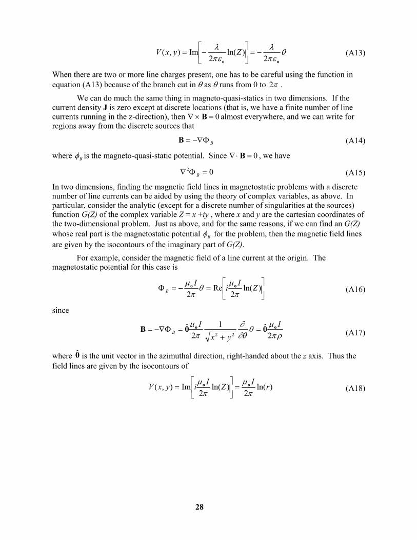


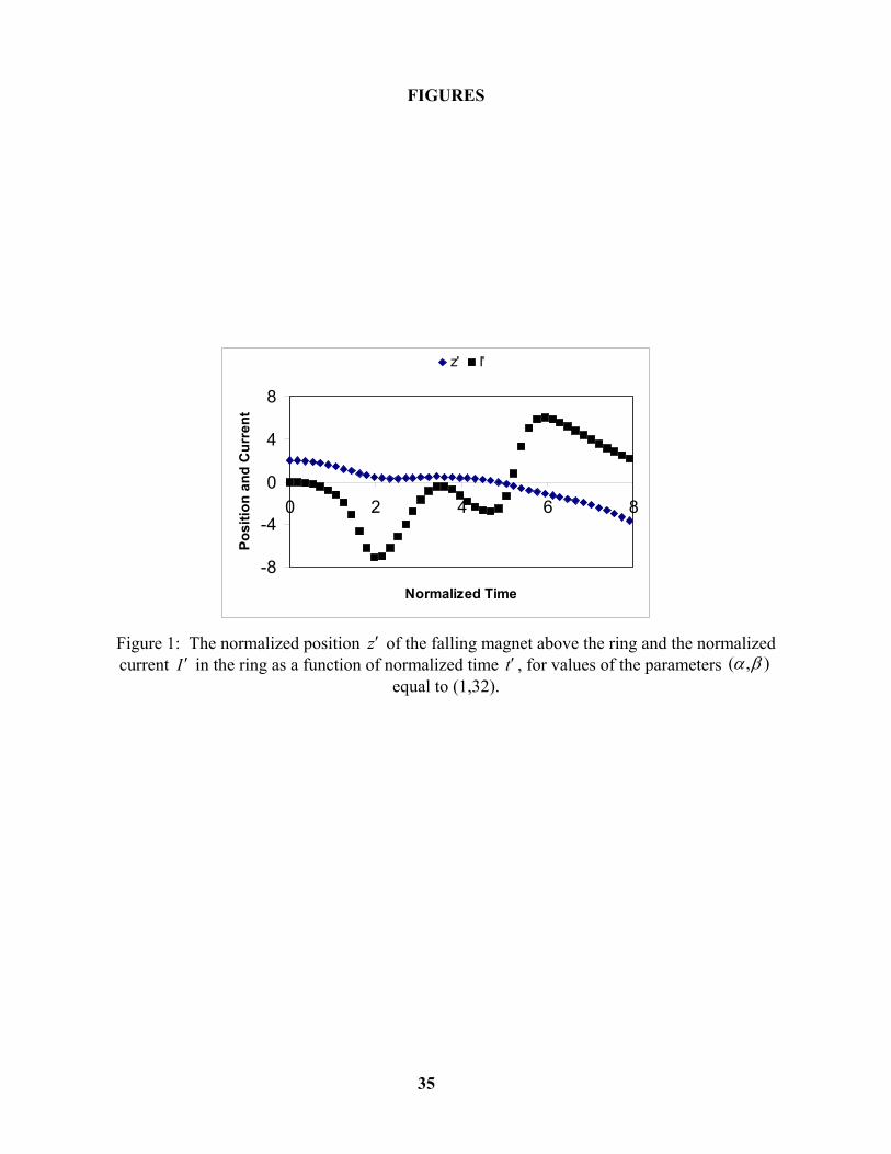
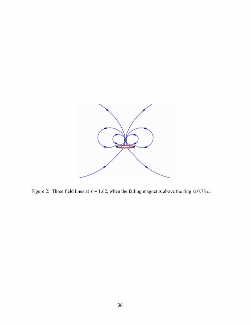


![[Wendy Laura Belcher] Writing Your Journal Article.](https://static.documents.pub/doc/80x56/577c7f921a28abe054a52463/wendy-laura-belcher-writing-your-journal-article.jpg)


