Variability in snow depth time series in the Adige catchment
Giorgia Marcolinia,b, Alberto Bellina, Markus Disseb, Gabriele Chiognab,c,⁎
a Department of Civil, Environmental and Mechanical Engineering, University of Trento, Via Mesiano 77, I-38123 Trento, Italyb Faculty of Civil, Geo and Environmental Engineering, Technical University of Munich, Arcistrasse 21, Munich 80333, Germanyc Institute of Geography, University of Innsbruck, Innrain 52, 6020 Innsbruck, Austria
A R T I C L E I N F O
Keywords:SnowClimate changeAlpsAdige catchment
A B S T R A C T
Study region: The Upper and Middle Adige catchment, Trentino-South Tyrol, Italy.Study focus: We provide evidence of changes in mean seasonal snow depth and snow coverduration in the region occurred in the period from 1980 to 2009.New hydrological insights for the region: Stations located above and below 1650m a.s.l. showdifferent dynamics, with the latter experiencing in the last decades a larger reduction of averagesnow depth and snow cover duration, than the former. Wavelet analyses show that snow dy-namics change with elevation and correlate differently with climatic indices at multiple temporalscales. We also observe that starting from the late 1980s snow cover duration and mean seasonalsnow depth are below the average in the study area. We also identify an elevation dependentcorrelation with the temperature. Moreover, correlation with the Mediterranean OscillationIndex and with the North Atlantic Oscillation Index is identified.
1. Introduction
Seasonal snow cover duration and mean seasonal snow depth have received significant attention in studies dealing with climatechange (Gobiet et al., 2014; Beniston and Stoffel, 2014), hydrology (Barnett et al., 2005; Berghuijs et al., 2014; Schneeberger et al.,2015), nitrogen and carbon cycle (Williams et al., 1998; Euskirchen et al., 2006), ecosystem functioning (Keller et al., 2005), soilprocesses (Groffman et al., 2001) and economy (Steiger and Stötter, 2013; Beniston, 2012a). Most of the existing studies focus on theSwiss and Austrian Alps (e.g. Beniston, 1997; Hantel et al., 2000; Schöner et al., 2009; Marty, 2008; Laternser and Schneebeli, 2003;Beniston et al., 2003). Much less attention has been devoted to the Southeastern Alps, in the Italian territory (Bocchiola and Rosso,2007; Valt and Cianfarra, 2010; Terzago et al., 2010; Pistocchi, 2016), despite the importance of snow dynamics in timing waterresources availability (Chiogna et al., 2016; Callegari et al., 2015), streamflow generation (Penna et al., 2013, 2017; Chiogna et al.,2014; Engel et al., 2016) and ecosystem functioning (Lencioni et al., 2011; Esposito et al., 2016).
In this paper, we analyze the dataset available covering the Adige catchment and five surrounding stations highly correlated withthose within this river basin. We focus on the period of 1980–2009, which is the richest of data for the area investigated.Furthermore, the analysis of snow dynamics in this time frame is of particular interest, since the 1990s have been an unusually warmand dry period for this region (Brunetti et al., 2009). Deepening the knowledge of snow dynamics South of the main Alpine ridge isrelevant because it is influenced by a meteorological circulation pattern that differs from the territories in the northern side of themountain chain (Xoplaki et al., 2004; Buzzi and Tibaldi, 1978). Owing to the different circulation patterns, different snow dynamicsmay be observed in the two regions, and the validity of the outcomes obtained for the Swiss and Austrian Alps does not necessarilyapply also to the Italian Alps. Moreover, the Adige catchment can be assumed as representative of the Southern Alpine ridge.
http://dx.doi.org/10.1016/j.ejrh.2017.08.007Received 1 June 2017; Received in revised form 21 July 2017; Accepted 24 August 2017
⁎ Corresponding author at: Faculty of Civil, Geo and Environmental Engineering, Technical University of Munich, Arcistrasse 21, Munich 80333, Germany.E-mail address: [email protected] (G. Chiogna).
Journal of Hydrology: Regional Studies 13 (2017) 240–254
First, we study the difference of the behavior of stations above and below 1650 m a.s.l. and the changes in mean seasonal snowdepth and snow cover duration occurred after 1987, showing that temperature changes may explain the observed snow dynamics, inparticular for low elevation sites. Then, we perform a wavelet analysis (Torrence and Compo, 1998) of the mean seasonal snow depthand of the snow cover duration at four elevation classes (below 1350 m a.s.l., between 1350 m a.s.l. and 1650 m a.s.l., between1650 m a.s.l. and 2000 m a.s.l. and above 2000 m a.s.l.). This allows us to identify changes occurring in the snow depth and snowcover duration signals at various temporal scales. Finally, we apply the wavelet coherence analysis (Grinsted et al., 2004) in order toinvestigate the relationship between the variations of the mean seasonal snow depth and that of climate indices such as the NorthAtlantic Oscillation Index (Hurrell, 1995) and the Mediterranean Oscillation Index (Palutikof, 2003). Several studies tried to link theNorth Atlantic Oscillation Index (NAOI) to the snow variability in order to explain it, however these results are not univocal (Scherrerand Appenzeller, 2006; Schöner et al., 2009; Scherrer et al., 2004; Durand et al., 2009; Beniston, 1997).
Section 2 describes the study area and the dataset available for this study, Section 3 is devoted to the description of the results,which are then discussed in Section 4, and finally Section 5 summarizes the conclusions.
2. Material and methods
2.1. Study area
The Adige catchment is one of the most important river basins in Italy, mainly for its large catchment area (12,100 km2) andlength (409 km) and for its hydropower generation. A recent review of Chiogna et al. (2016), described the hydrological conditions inthe catchment and its chemical and ecological status in details. The most important tributaries of the Adige catchment are located inthe Alpine part of the basin, and hence they are strongly influenced by snow dynamics (Mei et al., 2014; Tuo et al., 2016). Anincreasing concern is rising due to the effects of climate change in this area, since this has already shown important implications forwater resources management, and above all, for hydropower production and for winter tourism (Majone et al., 2016). In terms ofatmospheric circulation, the Adige catchment is mainly affected by southwest weather patterns and lee cyclones (Xoplaki et al., 2004;Buzzi and Tibaldi, 1978). Brunetti et al. (2006a, 2009) observed a slight negative trend in precipitation for the South Western area ofthe Greater Alpine Region. The Adige river basin belongs to this area, however, more recent studies, specifically addressing pre-cipitation trends in the river catchment (Lutz et al., 2016; Adler et al., 2015) did not identify significant trends. Moreover, Adler et al.(2015) indicates two additional drawbacks of the precipitation dataset available for the study area. The first is that very few stationsare available for elevations above 2000 m a.s.l. The second is the significant underestimation of winter precipitation due to un-dercatch of the rain gauges during snowstorms. Therefore, in this study we will not investigate the correlation between snow and theavailable precipitation dataset. Brunetti et al. (2006a,2009 observed a positive and statistically significant temperature trend in theriver basin. Moreover, the quality of the available time series was verified (see e.g. Adler et al., 2015). Therefore, we focus ouranalysis on the correlation between temperature and snow.
2.2. Description of the dataset
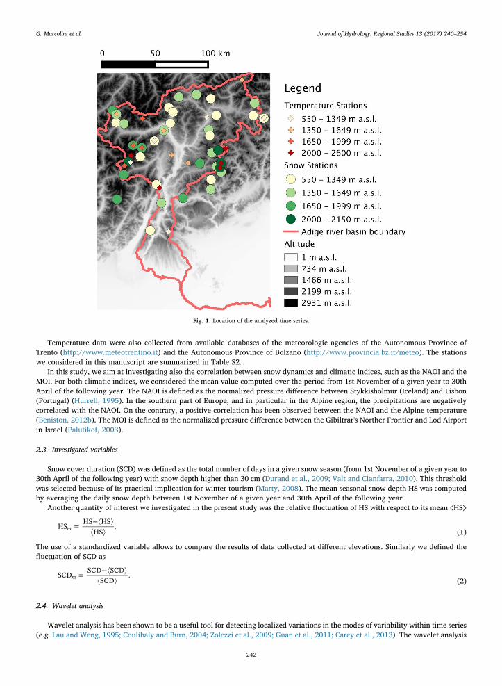
Snow depth time series of meteorological stations located in the Adige catchment are a relevant source of information to studysnow dynamics in the Alpine region (Fig. 1) because of their spatial distribution over a wide elevation range and time spanning. Inorder to extend the dataset as much as possible we included five additional stations (Malga Bissina, Caoria, Brocon – Marande, SanMartino di Castrozza and Sexten), which are outside the catchment, but very close to its boundaries. This choice was justified by thehigh correlation (r > 0.9) of the time series at similar elevations in this region. The dataset is therefore composed by 37 stations. Thestations have been grouped into four elevation classes, as shown in Table S1: below 1350 m a.s.l. (14 sites), between 1350 m and1650 m a.s.l. (12 sites), between 1650 m and 2000 m a.s.l. (7 sites) and above 2000 m a.s.l. (4 sites).
The dataset consists of daily data for the period 1st November–30th April between two successive years of the time series.Conventionally, we attributed this period to the starting year, e.g. the season 1990 is intended to be comprised between 1st November1990 and 30th April 1991. The time series may be formed by merging data obtained at stations which may have been relocatedduring the period from 1980 to 2009. Moreover, the time series are formed merging data from three different sources, according toquality indices criteria (Marcolini et al., 2017). Before the merging operation, we have checked the quality of the data. The highestquality index was assigned to manual data (measured from operators directly in the field), the second highest to automatic data(measured from automatic instruments), while historical data (collected from different sources, such as the Zentralanstalt für Me-teorologie und Geodynamik (ZAMG) of Vienna and the Hydrographic office of the Province of Trento) are considered the leastreliable, because measuring procedures and station locations are not always well documented. The merging of the data was per-formed to obtain single and longer time series for each site. Short gaps in the time series (i.e., shorter than 14 days), were filled bysupport vector machine regression (Smola and Schölkopf, 2004) performed by applying the Matlab toolbox Spider (http://www.kyb.tuebingen.mpg.de/bs/people/spider/), which uses the snow depth of the two best correlated stations and, if available, snowfall,temperature and precipitation data of the examined stations, as input variables for the regression.
Verifying the homogeneity of the time series is an important prerequisite for detecting trends and investigate climatic changes.Therefore, breakpoints in the time series (Auer et al., 2007; Brunetti et al., 2006a) caused by station relocation or merging of differentsources should be detected before carrying on further analyses. In this article, we only consider homogenous time series in the periodfrom 1980 to 2009. To check for homogeneity of available snow depth time series, we applied the Standard Normal HomogeneityTest (SNHT) (Alexandersson and Moberg, 1997; Alexandersson, 1986; Marcolini et al., 2017).
G. Marcolini et al. Journal of Hydrology: Regional Studies 13 (2017) 240–254
Temperature data were also collected from available databases of the meteorologic agencies of the Autonomous Province ofTrento (http://www.meteotrentino.it) and the Autonomous Province of Bolzano (http://www.provincia.bz.it/meteo). The stationswe considered in this manuscript are summarized in Table S2.
In this study, we aim at investigating also the correlation between snow dynamics and climatic indices, such as the NAOI and theMOI. For both climatic indices, we considered the mean value computed over the period from 1st November of a given year to 30thApril of the following year. The NAOI is defined as the normalized pressure difference between Stykkisholmur (Iceland) and Lisbon(Portugal) (Hurrell, 1995). In the southern part of Europe, and in particular in the Alpine region, the precipitations are negativelycorrelated with the NAOI. On the contrary, a positive correlation has been observed between the NAOI and the Alpine temperature(Beniston, 2012b). The MOI is defined as the normalized pressure difference between the Gibiltrar's Norther Frontier and Lod Airportin Israel (Palutikof, 2003).
2.3. Investigated variables
Snow cover duration (SCD) was defined as the total number of days in a given snow season (from 1st November of a given year to30th April of the following year) with snow depth higher than 30 cm (Durand et al., 2009; Valt and Cianfarra, 2010). This thresholdwas selected because of its practical implication for winter tourism (Marty, 2008). The mean seasonal snow depth HS was computedby averaging the daily snow depth between 1st November of a given year and 30th April of the following year.
Another quantity of interest we investigated in the present study was the relative fluctuation of HS with respect to its mean ⟨HS⟩
=−
HSHS HS
HS.m
(1)
The use of a standardized variable allows to compare the results of data collected at different elevations. Similarly we defined thefluctuation of SCD as
=−
SCDSCD SCD
SCD.m
(2)
2.4. Wavelet analysis
Wavelet analysis has been shown to be a useful tool for detecting localized variations in the modes of variability within time series(e.g. Lau and Weng, 1995; Coulibaly and Burn, 2004; Zolezzi et al., 2009; Guan et al., 2011; Carey et al., 2013). The wavelet analysis
Fig. 1. Location of the analyzed time series.
G. Marcolini et al. Journal of Hydrology: Regional Studies 13 (2017) 240–254
is performed by decomposing the time series into a transformed variable in time-frequency space to determine both the dominantmodes of variability and how these modes vary in time. We performed wavelet analysis by using the Matlab toolbox developed byTorrence and Compo (1998).
The continuous wavelet transform looks for similarity between a signal and a well-known mathematical function (Labat, 2005).The major difference to the Fourier transform, which is also the strength of this kind of analysis, is that the well-known mathematicalfunction, which for the wavelet analysis is a wavelet function, is applied several times with different scales to the analyzed time seriesand at different temporal positions. Wavelet transform allows us to determine not only the frequency content of a signal, as also theFourier analysis can do, but also the frequency time-dependence (Labat, 2005).
Similarly to other studies analyzing variability in climate and hydrological signals (see e.g. Lau and Weng, 1995; Coulibaly andBurn, 2004; Carey et al., 2013; Guan et al., 2011), the Morlet function was used as wavelet function for its ability to evidencefluctuations in time series.
The wavelet power spectrum (WPS), represents the energy of the scale s and is useful for the identification of fluctuation scaleswith the largest influence on the signal. In particular, a larger positive amplitude implies a higher positive correlation between thesignal and the wavelet and a large negative amplitude implies a high negative correlation.
The wavelet transform assumes that the time series is periodic. Since hydrological time series are not periodic and only a fractionof the entire time series is available, a bias is introduced at the beginning and at the end of the time series. To remove this bias,Torrence and Compo (1998) suggested to pad the end of the time series with zeros. The introduction of the zero padding (not shownin the pictures) leads to the definition of a cone of influence where edge effects are significant and hence the results are uncertain(Torrence and Compo, 1998). The cone of influence is indicated by shadowing the area of the contour plot showing the wavelettransform influenced by edge effects.
In our article, in particular, we considered the analysis of both the global wavelet power spectrum and the signal integrated from2 to 8 year scales. This allowed us to focus on the scales which lay within the cone of influence (i.e., results can be consideredstatistically significant), while filtering out the natural strong yearly periodicity of the snow signal.
Wavelet coherence (WTC) can be used to identify the scales where two time series X and Y focus on the power and how this maychange in time (Torrence and Compo, 1998; Grinsted et al., 2004).
Wavelet coherence can be interpreted as the generalization in the scale-time space of the squared cross-correlation coefficient r2 oftwo signals. Two time series display high coherence values (close to 1) for the time windows in which they are highly correlated.Similar to the classical correlation coefficient, when two time series display low coherence, the values are close to 0. The advantage ofwavelet coherence analysis with respect to classical correlation analysis is the possibility to identify separately for each scale thecoherence between two signals and eventually its variability over time. This allows us to identify at which scales and for which timewindows two signals are more correlated.
For more details about wavelet transform and wavelet coherence the reader is referred to Torrence and Compo (1998), Grinstedet al. (2004), Labat (2005) and Appendix A.
3. Results
3.1. Statistical analysis
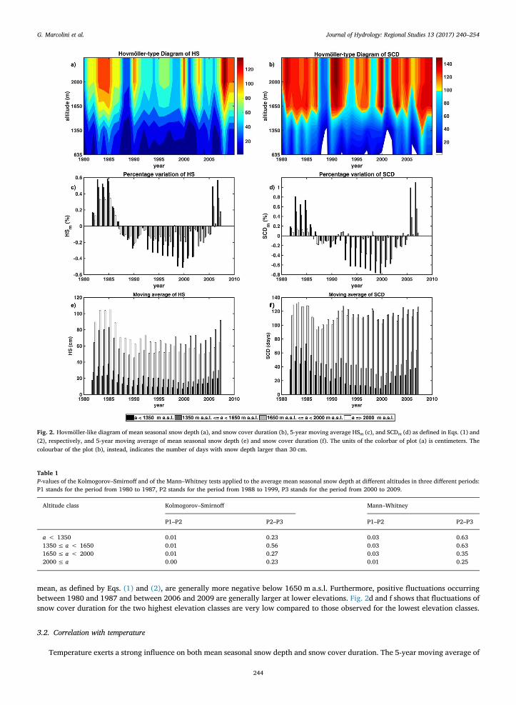
Fig. 2a and b shows an Hovmöller-like plot of the mean seasonal snow depth and of the snow cover duration at differentelevations. The diagrams display the two variables, using a color code, as a function of time and elevation which are reported in theabscissa and the ordinate, respectively. A sharp change in the color pattern occurs at about 1650 m a.s.l. Notice that the color map ofthe Hovmöller-like plot of the snow cover duration has two different colors at a threshold of 100 days with more than 30 cm of snowdepth during the winter season, since this is the level that is suggested to consider a site as economically profitable for winteractivities (Valt and Cianfarra, 2010). It can be observed that sites below 1650 m a.s.l. rarely reach this threshold value (7% of theseasons for the stations below 1350 m a.s.l. and 17% of the seasons for the stations between 1350 m and 1650 m a.s.l.).
Considering the temporal variability of snow depth (Fig. 2a), we identify three periods. The first one ranges from 1980 to 1987,the year in which Marty (2008) identified a regime shift (based on the sequential t-test analysis of regime shifts) in the snow coverduration in Switzerland. The second one (from 1988 to 1999) and the third one (from 2000 to 2009) are identified observing theincrease of the mean seasonal snow depth in Fig. 2a starting from 2000. To verify the statistical significance of our considerationsboth Kolmogorov–Smirnoff and Mann–Whitney tests have been conducted on mean seasonal snow depth data with a significancelevel of 5%. The results of the tests show that the period from 1988 to 1999 is characterized by significantly lower mean seasonalsnow depth than the period from 1980 to 1987 (see Table 1). On the contrary, in the period from 2000 to 2009, the increase of meanseasonal snow depth was not identified as statistically significant with respect to the period from 1988 to 1999 (see Table 1). Thesame analysis performed on snow cover duration time series identifies a statistically significant change of the two lowest elevationclasses (below 1650 m a.s.l.) and with 10% significance level (not shown).
Mean seasonal snow depth and snow cover duration have been analyzed considering also HSm and SCDm (Fig. 2c and d), and HSand SCD (Fig. 2e and f), aggregated according to the four elevation classes and smoothed using a 5-year moving average to eliminateshort term fluctuations. The choice of a 5-year moving average is appropriate considering the length of 30 years of the investigatedperiod and the length of the time intervals with low and high snow depth. The analysis of both mean seasonal snow depth and snowcover duration provided similar results. In Fig. 2c and d, it can be observed that stations located below 1650 m a.s.l. are affected by alarger variability than stations above 1650 m a.s.l. In particular, in the period from 1988 to 2005 fluctuations with respect to the
G. Marcolini et al. Journal of Hydrology: Regional Studies 13 (2017) 240–254
243
mean, as defined by Eqs. (1) and (2), are generally more negative below 1650 m a.s.l. Furthermore, positive fluctuations occurringbetween 1980 and 1987 and between 2006 and 2009 are generally larger at lower elevations. Fig. 2d and f shows that fluctuations ofsnow cover duration for the two highest elevation classes are very low compared to those observed for the lowest elevation classes.
3.2. Correlation with temperature
Temperature exerts a strong influence on both mean seasonal snow depth and snow cover duration. The 5-year moving average of
Fig. 2. Hovmöller-like diagram of mean seasonal snow depth (a), and snow cover duration (b), 5-year moving average HSm (c), and SCDm (d) as defined in Eqs. (1) and(2), respectively, and 5-year moving average of mean seasonal snow depth (e) and snow cover duration (f). The units of the colorbar of plot (a) is centimeters. Thecolourbar of the plot (b), instead, indicates the number of days with snow depth larger than 30 cm.
Table 1P-values of the Kolmogorov–Smirnoff and of the Mann–Whitney tests applied to the average mean seasonal snow depth at different altitudes in three different periods:P1 stands for the period from 1980 to 1987, P2 stands for the period from 1988 to 1999, P3 stands for the period from 2000 to 2009.
Altitude class Kolmogorov–Smirnoff Mann–Whitney
P1–P2 P2–P3 P1–P2 P2–P3
a < 1350 0.01 0.23 0.03 0.631350 ≤ a < 1650 0.01 0.56 0.03 0.631650 ≤ a < 2000 0.01 0.27 0.03 0.352000 ≤ a 0.00 0.23 0.01 0.25
G. Marcolini et al. Journal of Hydrology: Regional Studies 13 (2017) 240–254
244
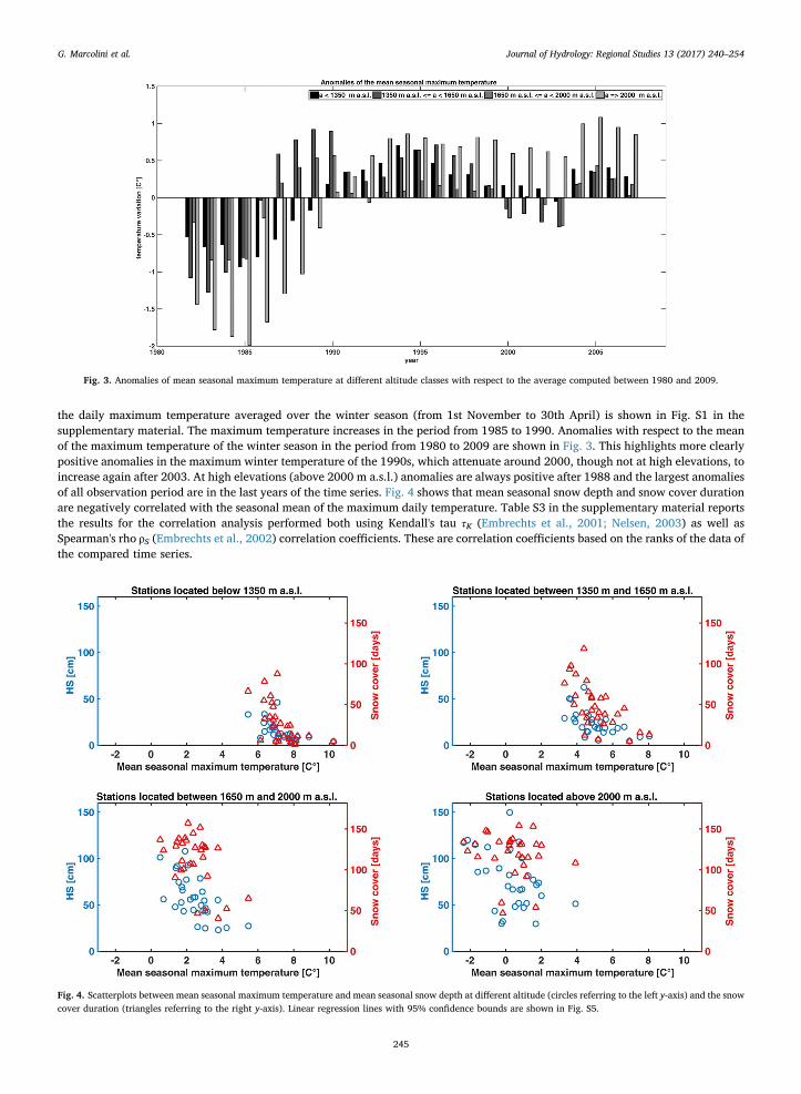
the daily maximum temperature averaged over the winter season (from 1st November to 30th April) is shown in Fig. S1 in thesupplementary material. The maximum temperature increases in the period from 1985 to 1990. Anomalies with respect to the meanof the maximum temperature of the winter season in the period from 1980 to 2009 are shown in Fig. 3. This highlights more clearlypositive anomalies in the maximum winter temperature of the 1990s, which attenuate around 2000, though not at high elevations, toincrease again after 2003. At high elevations (above 2000 m a.s.l.) anomalies are always positive after 1988 and the largest anomaliesof all observation period are in the last years of the time series. Fig. 4 shows that mean seasonal snow depth and snow cover durationare negatively correlated with the seasonal mean of the maximum daily temperature. Table S3 in the supplementary material reportsthe results for the correlation analysis performed both using Kendall's tau τK (Embrechts et al., 2001; Nelsen, 2003) as well asSpearman's rho ρS (Embrechts et al., 2002) correlation coefficients. These are correlation coefficients based on the ranks of the data ofthe compared time series.
Fig. 3. Anomalies of mean seasonal maximum temperature at different altitude classes with respect to the average computed between 1980 and 2009.
Fig. 4. Scatterplots between mean seasonal maximum temperature and mean seasonal snow depth at different altitude (circles referring to the left y-axis) and the snowcover duration (triangles referring to the right y-axis). Linear regression lines with 95% confidence bounds are shown in Fig. S5.
G. Marcolini et al. Journal of Hydrology: Regional Studies 13 (2017) 240–254
245
The negative correlation between temperature and HS is strongest for the stations located in the lowest elevation range(τK =−0.52 and ρS =−0.71) and decreases with increasing elevation (τK =−0.30 and ρS =−0.42 for the highest stations). Thedecrease in the values of the correlation coefficients with the altitude of the stations is even more evident when looking at the snowcover duration, for which we observe values varying from −0.54 to −0.15 for τK and values varying from −0.71 to −0.22 for ρS.
We also performed an hypothesis test of association with a confidence level of 95% based on the ρS and τK in order to verify thenull hypothesis that two variables are not correlated (Hollander and Wolfe, 1973; Best and Roberts, 1975). The results are shown inTable S4 and confirm in general the statistical significance of the correlation.
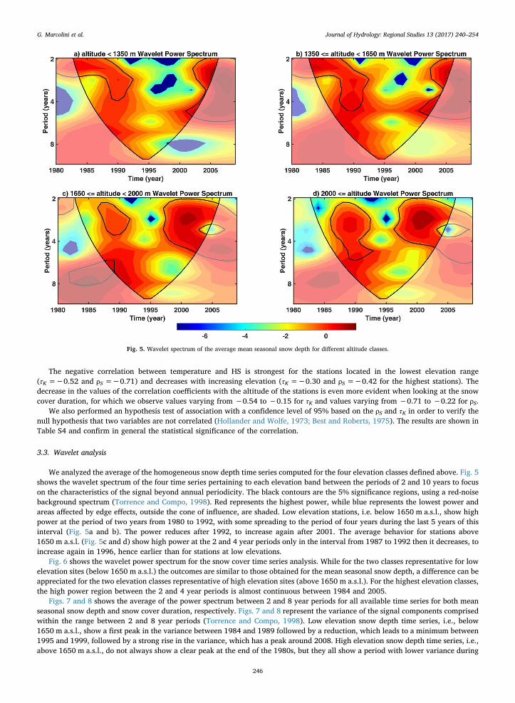
3.3. Wavelet analysis
We analyzed the average of the homogeneous snow depth time series computed for the four elevation classes defined above. Fig. 5shows the wavelet spectrum of the four time series pertaining to each elevation band between the periods of 2 and 10 years to focuson the characteristics of the signal beyond annual periodicity. The black contours are the 5% significance regions, using a red-noisebackground spectrum (Torrence and Compo, 1998). Red represents the highest power, while blue represents the lowest power andareas affected by edge effects, outside the cone of influence, are shaded. Low elevation stations, i.e. below 1650 m a.s.l., show highpower at the period of two years from 1980 to 1992, with some spreading to the period of four years during the last 5 years of thisinterval (Fig. 5a and b). The power reduces after 1992, to increase again after 2001. The average behavior for stations above1650 m a.s.l. (Fig. 5c and d) show high power at the 2 and 4 year periods only in the interval from 1987 to 1992 then it decreases, toincrease again in 1996, hence earlier than for stations at low elevations.
Fig. 6 shows the wavelet power spectrum for the snow cover time series analysis. While for the two classes representative for lowelevation sites (below 1650 m a.s.l.) the outcomes are similar to those obtained for the mean seasonal snow depth, a difference can beappreciated for the two elevation classes representative of high elevation sites (above 1650 m a.s.l.). For the highest elevation classes,the high power region between the 2 and 4 year periods is almost continuous between 1984 and 2005.
Figs. 7 and 8 shows the average of the power spectrum between 2 and 8 year periods for all available time series for both meanseasonal snow depth and snow cover duration, respectively. Figs. 7 and 8 represent the variance of the signal components comprisedwithin the range between 2 and 8 year periods (Torrence and Compo, 1998). Low elevation snow depth time series, i.e., below1650 m a.s.l., show a first peak in the variance between 1984 and 1989 followed by a reduction, which leads to a minimum between1995 and 1999, followed by a strong rise in the variance, which has a peak around 2008. High elevation snow depth time series, i.e.,above 1650 m a.s.l., do not always show a clear peak at the end of the 1980s, but they all show a period with lower variance during
Fig. 5. Wavelet spectrum of the average mean seasonal snow depth for different altitude classes.
G. Marcolini et al. Journal of Hydrology: Regional Studies 13 (2017) 240–254
246
the 1990s. Also high elevation sites show a peak after the 1990s, but it starts around 2000, hence anticipating the one observed forstations below 1650 m a.s.l., which starts after 2003. Overall, variations in the variance of the signal are more moderate at higherelevations. A similar pattern can be identified for snow cover duration, as shown in Fig. 8. The main difference can be observed forhigh elevation sites, where the reduction of the variance occurred in the 1990s is less pronounced than in the analysis of the meanseasonal snow depth signal.
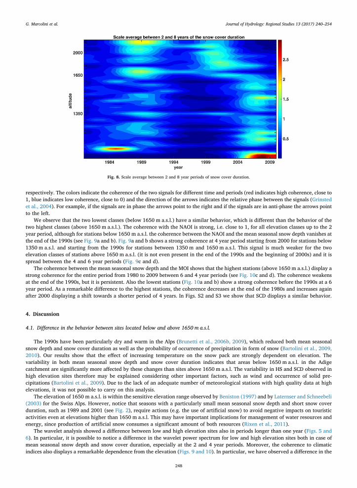
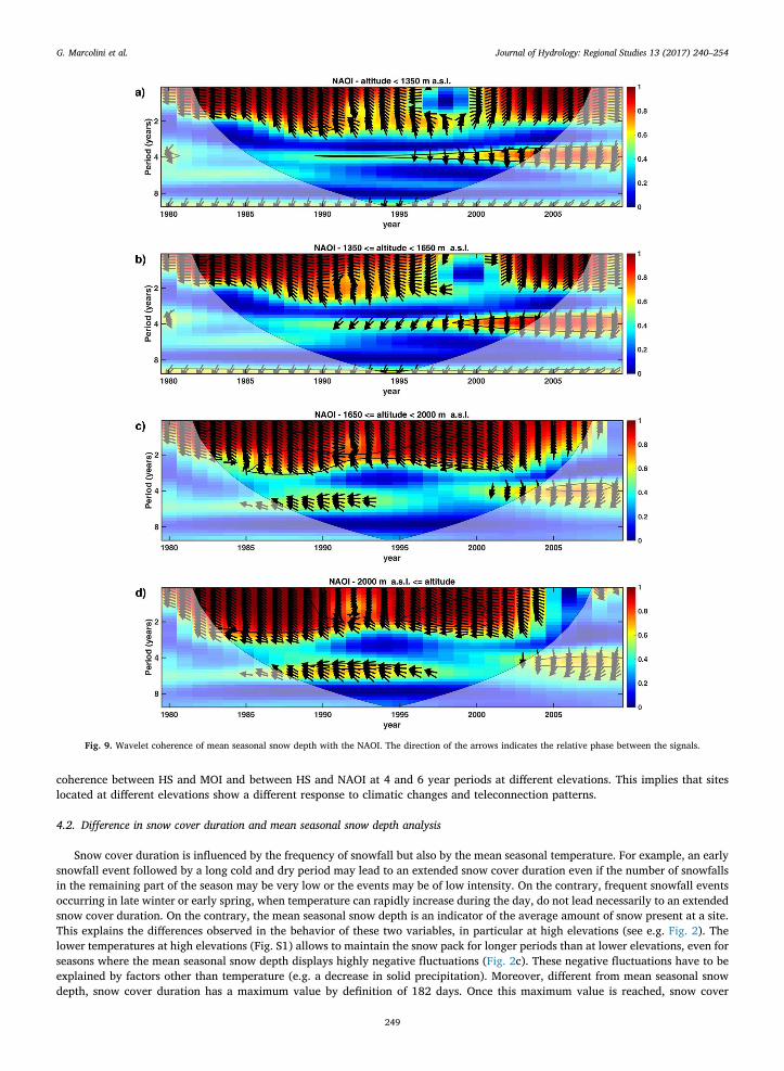
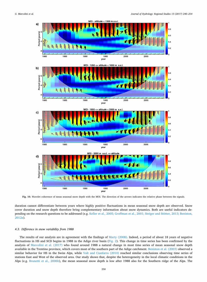
Coherence between mean seasonal snow depth at different elevations and the NAOI and the MOI is shown in Figs. 9 and 10,
Fig. 6. Wavelet spectrum of the average snow cover for different altitude classes.
Fig. 7. Scale average between 2 and 8 year periods of mean seasonal snow depth.
G. Marcolini et al. Journal of Hydrology: Regional Studies 13 (2017) 240–254
247
respectively. The colors indicate the coherence of the two signals for different time and periods (red indicates high coherence, close to1, blue indicates low coherence, close to 0) and the direction of the arrows indicates the relative phase between the signals (Grinstedet al., 2004). For example, if the signals are in phase the arrows point to the right and if the signals are in anti-phase the arrows pointto the left.
We observe that the two lowest classes (below 1650 m a.s.l.) have a similar behavior, which is different than the behavior of thetwo highest classes (above 1650 m a.s.l.). The coherence with the NAOI is strong, i.e. close to 1, for all elevation classes up to the 2year period, although for stations below 1650 m a.s.l. the coherence between the NAOI and the mean seasonal snow depth vanishes atthe end of the 1990s (see Fig. 9a and b). Fig. 9a and b shows a strong coherence at 4 year period starting from 2000 for stations below1350 m a.s.l. and starting from the 1990s for stations between 1350 m and 1650 m a.s.l. This signal is much weaker for the twoelevation classes of stations above 1650 m a.s.l. (it is not even present in the end of the 1990s and the beginning of 2000s) and it isspread between the 4 and 6 year periods (Fig. 9c and d).
The coherence between the mean seasonal snow depth and the MOI shows that the highest stations (above 1650 m a.s.l.) display astrong coherence for the entire period from 1980 to 2009 between 6 and 4 year periods (see Fig. 10c and d). The coherence weakensat the end of the 1990s, but it is persistent. Also the lowest stations (Fig. 10a and b) show a strong coherence before the 1990s at a 6year period. As a remarkable difference to the highest stations, the coherence decreases at the end of the 1980s and increases againafter 2000 displaying a shift towards a shorter period of 4 years. In Figs. S2 and S3 we show that SCD displays a similar behavior.
4. Discussion
4.1. Difference in the behavior between sites located below and above 1650 m a.s.l.
The 1990s have been particularly dry and warm in the Alps (Brunetti et al., 2006b, 2009), which reduced both mean seasonalsnow depth and snow cover duration as well as the probability of occurrence of precipitation in form of snow (Bartolini et al., 2009,2010). Our results show that the effect of increasing temperature on the snow pack are strongly dependent on elevation. Thevariability in both mean seasonal snow depth and snow cover duration indicates that areas below 1650 m a.s.l. in the Adigecatchment are significantly more affected by these changes than sites above 1650 m a.s.l. The variability in HS and SCD observed inhigh elevation sites therefore may be explained considering other important factors, such as wind and occurrence of solid pre-cipitations (Bartolini et al., 2009). Due to the lack of an adequate number of meteorological stations with high quality data at highelevations, it was not possible to carry on this analysis.
The elevation of 1650 m a.s.l. is within the sensitive elevation range observed by Beniston (1997) and by Laternser and Schneebeli(2003) for the Swiss Alps. However, notice that seasons with a particularly small mean seasonal snow depth and short snow coverduration, such as 1989 and 2001 (see Fig. 2), require actions (e.g. the use of artificial snow) to avoid negative impacts on touristicactivities even at elevations higher than 1650 m a.s.l. This may have important implications for management of water resources andenergy, since production of artificial snow consumes a significant amount of both resources (Rixen et al., 2011).
The wavelet analysis showed a difference between low and high elevation sites also in periods longer than one year (Figs. 5 and6). In particular, it is possible to notice a difference in the wavelet power spectrum for low and high elevation sites both in case ofmean seasonal snow depth and snow cover duration, especially at the 2 and 4 year periods. Moreover, the coherence to climaticindices also displays a remarkable dependence from the elevation (Figs. 9 and 10). In particular, we have observed a difference in the
Fig. 8. Scale average between 2 and 8 year periods of snow cover duration.
G. Marcolini et al. Journal of Hydrology: Regional Studies 13 (2017) 240–254
248
coherence between HS and MOI and between HS and NAOI at 4 and 6 year periods at different elevations. This implies that siteslocated at different elevations show a different response to climatic changes and teleconnection patterns.
4.2. Difference in snow cover duration and mean seasonal snow depth analysis
Snow cover duration is influenced by the frequency of snowfall but also by the mean seasonal temperature. For example, an earlysnowfall event followed by a long cold and dry period may lead to an extended snow cover duration even if the number of snowfallsin the remaining part of the season may be very low or the events may be of low intensity. On the contrary, frequent snowfall eventsoccurring in late winter or early spring, when temperature can rapidly increase during the day, do not lead necessarily to an extendedsnow cover duration. On the contrary, the mean seasonal snow depth is an indicator of the average amount of snow present at a site.This explains the differences observed in the behavior of these two variables, in particular at high elevations (see e.g. Fig. 2). Thelower temperatures at high elevations (Fig. S1) allows to maintain the snow pack for longer periods than at lower elevations, even forseasons where the mean seasonal snow depth displays highly negative fluctuations (Fig. 2c). These negative fluctuations have to beexplained by factors other than temperature (e.g. a decrease in solid precipitation). Moreover, different from mean seasonal snowdepth, snow cover duration has a maximum value by definition of 182 days. Once this maximum value is reached, snow cover
Fig. 9. Wavelet coherence of mean seasonal snow depth with the NAOI. The direction of the arrows indicates the relative phase between the signals.
G. Marcolini et al. Journal of Hydrology: Regional Studies 13 (2017) 240–254
249
duration cannot differentiate between years where highly positive fluctuations in mean seasonal snow depth are observed. Snowcover duration and snow depth therefore bring complementary information about snow dynamics. Both are useful indicators de-pending on the research questions to be addressed (e.g. Keller et al., 2005; Groffman et al., 2001; Steiger and Stötter, 2013; Beniston,2012a).
4.3. Difference in snow variability from 1988
The results of our analysis are in agreement with the findings of Marty (2008). Indeed, a period of about 18 years of negativefluctuations in HS and SCD begins in 1988 in the Adige river basin (Fig. 2). This change in time series has been confirmed by theanalysis of Marcolini et al. (2017) who found around 1988 a natural change in most time series of mean seasonal snow depthavailable in the Trentino province, which covers most of the southern part of the Adige catchment. Beniston et al. (2003) observed asimilar behavior for HS in the Swiss Alps, while Valt and Cianfarra (2010) reached similar conclusions observing time series ofstations East and West of the observed area. Our study shows that, despite the heterogeneity in the local climatic conditions in theAlps (e.g. Brunetti et al., 2006b), the mean seasonal snow depth is low after 1988 also for the Southern ridge of the Alps. The
Fig. 10. Wavelet coherence of mean seasonal snow depth with the MOI. The direction of the arrows indicates the relative phase between the signals.
G. Marcolini et al. Journal of Hydrology: Regional Studies 13 (2017) 240–254
250
variability in mean seasonal snow depth is mainly controlled by the interplay between the observed increasing temperatures and theatmospheric pressure in the Alps (Brunetti et al., 2009). The correlation between temperature anomalies and mean seasonal snowdepth shown in Fig. 4 therefore supports the hypothesis that temperature is one of the main driving factors of the observed change insnow dynamics in the Alpine Region in particular at low elevation sites (Scherrer et al., 2004).
The observed snow cover duration in our study area is consistent with the observations performed both in other sites in NorthernItaly (Valt and Cianfarra, 2010) and Switzerland (Laternser and Schneebeli, 2003; Marty, 2008). Also for this variable, the short term(seasonal) variability strongly depends on local site specific conditions (Marty, 2008). However, our study shows that long termvariability is controlled by global climate forcing factors, common for different regions of the Alps (e.g. Beniston, 1997; Marty, 2008;Valt and Cianfarra, 2010).
In order to evaluate the correlation of the variability of mean seasonal snow depth to global climate forcing factors, we analyzedits coherence with two oscillation indices: the NAOI and the MOI (Figs. 9 and 10). We cannot observe a clear relationship between thevariations of the coherence between the NAOI and mean seasonal snow depth in the Adige River Basin and the changes observed inthe behavior of snow in the last decades at periods longer than 2 years. In particular, the patterns observed for different elevations aredifferent and do not reproduce the behavior observed for the anomalies in mean seasonal snow depth (decrease in the 1990s andincrease, although not statistically significant, since 2000). The behavior shown in Fig. 10, instead, shows a change in the coherencebetween mean seasonal snow depth and the MOI at periods of 4–6 years during the 1990s. This is in accordance with the patternsobserved for both mean seasonal snow depth and snow cover duration. The modification of this coherence during the 1990s, incorrespondence with the period of the decrease of mean seasonal snow depth and snow cover duration, suggests a correlationbetween the MOI and the reduction of snow in the analyzed time period. The phase shift indicates that when the MOI and the snowsignal display a strong coherence, they are almost anticorrelated. Moreover, the intensity of this change is stronger for stations below1650 m a.s.l., confirming the higher sensitivity of these sites towards climate changes. In fact, for those stations we observe a break ofthe coherence during the 1990s, while for stations above 1650 m a.s.l. the coherence only decreases in this decade. In particular, theelevation dependence of the coherence between the mean seasonal snow depth and the MOI is highlighted in Fig. 10, where for thescales of 2 and 4 years the coherence for the stations below 1650 m a.s.l. reaches values close to 0.3 or even smaller than 0.2, whilefor stations above 1650 m a.s.l. the coherence does not reach values smaller than 0.5.
5. Conclusions
In this article, we analyzed the snow depth time series in the Adige catchment (North-East Italy) for the period from 1980 to 2009.Our results show that the Adige catchment experienced a significant reduction of both snow cover duration and mean seasonal snowdepth after 1988. This reduction is observed both at low and high elevation sites, although we can distinguish between the behaviorof the time series located above and below 1650 m a.s.l. In particular, low elevation sites are more affected by climate variability andmore sensitive to temperature increase than high elevation sites. The difference between high and low elevation sites is also con-firmed by the wavelet analysis. We also observe that in the analyzed period the coherence between mean seasonal snow depth signaland the MOI is low when mean seasonal snow depth is low at the scale between 4 and 8 years.
Due to the relevance of snow dynamics for other environmental processes, this study can provide an important reference for theexplanation of changes, such as temporal shifts in streamflow peak, touristic and chemical fluxes, observed in this region in the pastdecades.
Conflict of interest
All authors declare that they have no conflict of interest.
Acknowledgments
We thank two anonymous reviewers for the comments that helped improving the manuscript. This research was partially sup-ported by the European Communities 7th Framework Programme under Grant Agreement No. 603629-ENV-2013-6.2.1-Globaquaand by the German Research Foundation (DFG) and the Technische Universität München within the Open Access Publishing FundingProgramme. G.C. acknowledges the support of the Stiftungsfonds für Umweltökonomie und Nachhaltigkeit GmbH (SUN). The authorswould like to acknowledge meteorological survey of the Province of Trento Meteotrentino and of the Province of Bolzano for pro-viding the data and for the collaboration. Any opinions, conclusions, or recommendations expressed in this manuscript are solelythose of the authors and do not necessarily reflect the views of the supporting agencies.
Appendix A. Supplementary data
Supplementary data associated with this article can be found, in the online version, at http://dx.doi.org/10.1016/j.ejrh.2017.08.007.
Appendix A. Wavelet analysis
The continuous wavelet transformation of a discretized signal xn, n = 1, …, N, sampled at the time interval δt, is defined as
G. Marcolini et al. Journal of Hydrology: Regional Studies 13 (2017) 240–254
where ψ(η) is a band-pass filter and the superscript * indicates the complex conjugate. Mathematically, the transform in Eq. (A.1) isthe convolution of the signal xn with the scaled version of the wavelet function ψ, which is obtained from a “mother wavelet” ψo(η),normalized at each scale s to fulfill the following condition:
∑ ==
−
ψ s ω N| ( )|k
N
k0
12
(A.2)
where ωk = 2πk/(Nδt) for k≤ N/2, and ωk =−2πk/(Nδt) for k > N/2 is the angular frequency and s is the wavelet scale (Torrenceand Compo, 1998). In this study, the Morlet function was used as “mother wavelet” and it is defined as:
= − −ψ η π e e( )oi ω η η1/4 /2o 2
(A.3)
where ωo is the dimensionless frequency (Grinsted et al., 2004) and η is the dimensionless time. Following Torrence and Compo(1998) ωo is set to 6. In this way the wavelet scale is almost identical to the corresponding Fourier period.
The wavelet transform of Eq. (A.1) is computed for a selection of scales:
= = …s s j J, 1, 2, ,jj δ
02 j (A.4)
where s0 is the smallest scale considered in the analysis and = −J δ Nδ slog ( / )j t1
2 0 determines the largest scale. Moreover, δj is theinverse of the number of scales per each octave, i.e. the distance between one frequency and its double. In addition, s0 should bechosen in order to make the equivalent Fourier period approximately 2 δt.
The wavelet power spectrum (WPS) is defined as the product of wavelet transform, Wn(s), by its conjugate, W * n(s).The Wavelet coherence (WTC) between two time series X and Y with wavelet transformsW s( )n
X andW s( )nY , respectively, is defined
as (Torrence and Compo, 1998; Grinsted et al., 2004):
=−
− −R sS s W s
S s W s S s W s( )
| [ ( )]|[ | ( )| ] [ | ( )| ]n
n
nX
nY
21 XY 2
1 2 1 2 (A.5)
where =W s W s W s( ) ( ) * ( )n nX
nYXY , where the superscript * indicates the complex conjugate, S is a smoothing operator, given by
=S W S S W s( ) { [ ( )]}nscale time (A.6)
where Sscale denotes smoothing with respect to the scales s and Stime smoothing in time. For the Morlet wavelet Torrence and Compo(1998) suggested the following smoothing operator:
==
−S W W s cS W W s c s
( )| ( ( )* )| ,( )| ( ( )* Π(0.6 ))|
s nt s
s
s n n
time 1/2
time 2
2 2
(A.7)
where c1 and c2 are normalization constants and Π is the step function. The factor 0.6 is the empirically determined scale decorr-elation length for the Morlet wavelet (see Torrence and Compo, 1998).
References
Adler, S., Chimani, B., Drechsel, S., Haslinger, K., Hiebl, J., Meyer, V., Resch, G., Rudolph, J., Vergeiner, J., Zingerle, C., Marigo, G., Fischer, A., Seiser, B., 2015. Ilclima del Tirolo – Alto Adige – Bellunese. Zentralanstalt fur Meteorologie und Geodynamik (ZAMG), Ripartizione Protezione antincendi e civile – ProvinciaAutonoma di Bolzano, Agenzia Regionale per la Prevenzione e Protezione Ambientale del Veneto (ARPAV).Il clima del Tirolo – Alto Adige – Bellunese.Zentralanstalt fur Meteorologie und Geodynamik (ZAMG), Ripartizione Protezione antincendi e civile – Provincia Autonoma di Bolzano, Agenzia Regionale per laPrevenzione e Protezione Ambientale del Veneto (ARPAV).
Alexandersson, H., 1986. A homogeneity test applied to precipitation data. J. Climatol. 6 (6), 661–675.Alexandersson, H., Moberg, A., 1997. Homogenization of Swedish temperature data: Part I. Homogeneity test for linear trends. Int. J. Climatol. 17 (1), 25–34.Auer, I., Böhm, R., Jurkovic, A., Lipa, W., Orlik, A., Potzmann, R., Schöner, W., Ungersböck, M., Matulla, C., Briffa, K., et al., 2007. Histalp-historical instrumental
climatological surface time series of the Greater Alpine Region. Int. J. Climatol. 27 (1), 17–46.Barnett, T.P., Adam, J.C., Lettenmaier, D.P., 2005. Potential impacts of a warming climate on water availability in snow-dominated regions. Nature 438 (7066),
303–309.Bartolini, E., Claps, P., D’Odorico, P., 2009. Interannual variability of winter precipitation in the European Alps: relations with the North Atlantic Oscillation. Hydrol.
Earth Syst. Sci. 13 (1), 17–25.Bartolini, E., Claps, P., D’Odorico, P., 2010. Connecting European snow cover variability with large scale atmospheric patterns. Adv. Geosci. 26 (26), 93–97.Beniston, M., 1997. Variations of snow depth and duration in the Swiss Alps over the last 50 years: links to changes in large-scale climatic forcings. Clim. Change 36 (3-
4), 281–300.Beniston, M., 2012a. Impacts of climatic change on water and associated economic activities in the Swiss Alps. J. Hydrol. 412, 291–296.Beniston, M., 2012b. Is snow in the Alps receding or disappearing? Wiley Interdiscip. Rev. Clim. Change 3 (4), 349–358.Beniston, M., Keller, F., Goyette, S., 2003. Snow pack in the Swiss Alps under changing climatic conditions: an empirical approach for climate impacts studies. Theor.
Appl. Climatol. 74 (1-2), 19–31.Beniston, M., Stoffel, M., 2014. Assessing the impacts of climatic change on mountain water resources. Sci. Total Environ. 493 (0), 1129–1137. http://www.
Berghuijs, W., Woods, R., Hrachowitz, M., 2014. A precipitation shift from snow towards rain leads to a decrease in streamflow. Nat. Clim. Change 4 (7), 583–586.Best, D., Roberts, D., 1975. Algorithm as 89: the upper tail probabilities of spearman's rho. J. R. Stat. Soc. Ser. C: Appl. Stat. 24 (3), 377–379.Bocchiola, D., Rosso, R., 2007. The distribution of daily snow water equivalent in the Central Italian Alps. Adv. Water Resour. 30 (1), 135–147.Brunetti, M., Lentini, G., Maugeri, M., Nanni, T., Auer, I., Böhm, R., Schöner, W., 2009. Climate variability and change in the Greater Alpine Region over the last two
centuries based on multi-variable analysis. Int. J. Climatol. 29 (15), 2197–2225. http://dx.doi.org/10.1002/joc.1857.Brunetti, M., Maugeri, M., Monti, F., Nanni, T., 2006a. Temperature and precipitation variability in Italy in the last two centuries from homogenised instrumental time
series. Int. J. Climatol. 26 (3), 345–381.Brunetti, M., Maugeri, M., Nanni, T., Auer, I., Böhm, R., Schöner, W., 2006b. Precipitation variability and changes in the Greater Alpine Region over the 1800–2003
period. J. Geophys. Res. Atmos. 111 (D11). http://dx.doi.org/10.1029/2005JD006674.Buzzi, A., Tibaldi, S., 1978. Cyclogenesis in the lee of the Alps: a case study. Quart. J. R. Meteorol. Soc. 104 (440), 271–287.Callegari, M., Mazzoli, P., de Gregorio, L., Notarnicola, C., Pasolli, L., Petitta, M., Pistocchi, A., 2015. Seasonal river discharge forecasting using support vector
regression: a case study in the Italian Alps. Water Switz. 7 (5), 2494–2515.Carey, S.K., Tetzlaff, D., Buttle, J., Laudon, H., McDonnell, J., McGuire, K., Seibert, J., Soulsby, C., Shanley, J., 2013. Use of color maps and wavelet coherence to
discern seasonal and interannual climate influences on streamflow variability in northern catchments. Water Resour. Res. 49 (10), 6194–6207.Chiogna, G., Majone, B., Paoli, K.C., Diamantini, E., Stella, E., Mallucci, S., Lencioni, V., Zandonai, F., Bellin, A., 2016. A review of hydrological and chemical stressors
in the Adige catchment and its ecological status. Sci. Total Environ. 540, 429–443. 5th Special Issue SCARCE: River Conservation under Multiple Stressors:Integration of Ecological Status, Pollution and Hydrological Variability. http://www.sciencedirect.com/science/article/pii/S0048969715303430.
Chiogna, G., Santoni, E., Camin, F., Tonon, A., Majonea, B., Trenti, A., Bellin, A., 2014. Stable Isotope Characterization of the Vermigliana Catchment. J. Hydrol. 509,295–305.
Coulibaly, P., Burn, D.H., 2004. Wavelet analysis of variability in annual Canadian streamflows. Water Resour. Res. 40 (3).Durand, Y., Giraud, G., Laternser, M., Etchevers, P., Mérindol, L., Lesaffre, B., 2009. Reanalysis of 47 years of climate in the French Alps (1958–2005): climatology and
trends for snow cover. J. Appl. Meteorol. Climatol. 48 (12), 2487–2512.Embrechts, P., Lindskog, F., McNeil, A., 2001. Modelling Dependence with Copulas. Rapport Technique. Département de mathématiques, Institut Fédéral de
Technologie de Zurich, Zurich.Embrechts, P., McNeil, A., Straumann, D., 2002. Correlation and dependence in risk management: properties and pitfalls. Risk Management: Value at Risk and Beyond.
pp. 176223.Engel, M., Penna, D., Bertoldi, G., Dell’Agnese, A., Soulsby, C., Comiti, F., 2016. Identifying run-off contributions during melt-induced run-off events in a glacierized
alpine catchment. Hydrol. Process. 30 (3), 343–364.Esposito, A., Engel, M., Ciccazzo, S., Daprà, L., Penna, D., Comiti, F., Zerbe, S., Brusetti, L., 2016. Spatial and temporal variability of bacterial communities in high
alpine water spring sediments. Res. Microbiol. 167 (4), 325–333.Euskirchen, E., McGuire, A.D., Kicklighter, D.W., Zhuang, Q., Clein, J.S., Dargaville, R., Dye, D., Kimball, J.S., McDonald, K.C., Melillo, J.M., et al., 2006. Importance of
recent shifts in soil thermal dynamics on growing season length, productivity, and carbon sequestration in terrestrial high-latitude ecosystems. Glob. Change Biol.12 (4), 731–750.
Gobiet, A., Kotlarski, S., Beniston, M., Heinrich, G., Rajczak, J., Stoffel, M., 2014. 21st century climate change in the European Alps: a review. Sci. Total Environ. 493(0), 1138–1151. http://www.sciencedirect.com/science/article/pii/S0048969713008188.
Grinsted, A., Moore, J.C., Jevrejeva, S., 2004. Application of the cross wavelet transform and wavelet coherence to geophysical time series. Nonlinear Process.Geophys. 11 (5/6), 561–566.
Groffman, P., Driscoll, C., Fahey, T., Hardy, J., Fitzhugh, R., Tierney, G., 2001. Colder soils in a warmer world: a snow manipulation study in a northern hardwoodforest ecosystem. Biogeochemistry 56 (2), 135–150. http://dx.doi.org/10.1023/A3A1013039830323.
Guan, K., Thompson, S.E., Harman, C.J., Basu, N.B., Rao, P.S.C., Sivapalan, M., Packman, A.I., Kalita, P.K., 2011. Spatiotemporal scaling of hydrological and agro-chemical export dynamics in a tile-drained midwestern watershed. Water Resour. Res. 47 (10). http://dx.doi.org/10.1029/2010WR009997.
Hantel, M., Ehrendorfer, M., Haslinger, A., et al., 2000. Climate sensitivity of snow cover duration in Austria. Int. J. Climatol. 20 (6), 615–640.Hollander, M., Wolfe, D.A., 1973. Nonparametric Statistical Methods. John Wiley & Sons.Hurrell, J.W., 1995. Decadal trends in the North Atlantic Oscillation: regional temperatures and precipitation. Science 269 (5224), 676–679.Keller, F., Goyette, S., Beniston, M., 2005. Sensitivity analysis of snow cover to climate change scenarios and their impact on plant habitats in alpine terrain. Clim.
Change 72 (3), 299–319. http://dx.doi.org/10.1007/s10584-005-5360-2.Labat, D., 2005. Recent advances in wavelet analyses: Part 1. A review of concepts. J. Hydrol. 314 (1), 275–288.Laternser, M., Schneebeli, M., 2003. Long-term snow climate trends of the Swiss Alps (1931–99). Int. J. Climatol. 23 (7), 733–750.Lau, K.M., Weng, H., 1995. Climate signal detection using wavelet transform: how to make a time series sing. Bull. Am. Meteorol. Soc. 76, 2391–2402.Lencioni, V., Marziali, L., Rossaro, B., 2011. Diversity and distribution of chironomids (Diptera, Chironomidae) in pristine Alpine and pre-Alpine springs (Northern
Italy). J. Limnol. 70 (1s), 106–121.Lutz, S.R., Mallucci, S., Diamantini, E., Majone, B., Bellin, A., Merz, R., 2016. Hydroclimatic and water quality trends across three Mediterranean river basins. Sci. Total
Environ. 571, 1392–1406.Majone, B., Villa, F., Deidda, R., Bellin, A., 2016. Impact of climate change and water use policies on hydropower potential in the south-eastern alpine region. Sci. Total
Environ. 543, 965–980.Marcolini, G., Bellin, A., Chiogna, G., 2017. Performance of the standard normal homogeneity test for the homogenization of mean seasonal snow depth time series.
Int. J. Climatol.Marty, C., 2008. Regime shift of snow days in Switzerland. Geophys. Res. Lett. 35 (12), l12501. http://dx.doi.org/10.1029/2008GL033998.Mei, Y., Anagnostou, E.N., Nikolopoulos, E.I., Borga, M., 2014. Error analysis of satellite precipitation products in mountainous basins. J. Hydrometeorol. 15 (5),
1778–1793.Nelsen, R.B., 2003. Properties and applications of copulas: a brief survey. In: Dhaene, J., Kolev, N., Morettin, P.A. (Eds.), Proceedings of the First Brazilian Conference
on Statistical Modeling in Insurance and Finance. University Press USP, Sao Paulo, pp. 10–28 (Citeseer).Palutikof, J., 2003. Analysis of Mediterranean climate data: measured and modelled. Mediterranean Climate. Springer, pp. 125–132.Penna, D., Engel, M., Bertoldi, G., Comiti, F., 2017. Towards a tracer-based conceptualization of meltwater dynamics and streamflow response in a glacierized
catchment. Hydrol. Earth Syst. Sci. 21 (1), 23.Penna, D., Mao, L., Comiti, F., Engel, M., Dell’Agnese, A., Bertoldi, G., 2013. Hydrological effects of glacier melt and snowmelt in a high-elevation catchment.
Bodenkultur 64 (3–4), 93–98.Pistocchi, A., 2016. Simple estimation of snow density in an alpine region. J. Hydrol. Reg. Stud. 6, 82–89.Rixen, C., Teich, M., Lardelli, C., Gallati, D., Pohl, M., Pütz, M., Bebi, P., 2011. Winter tourism and climate change in the Alps: an assessment of resource consumption,
snow reliability, and future snowmaking potential. Mt. Res. Dev. 31 (3), 229–236.Scherrer, S.C., Appenzeller, C., 2006. Swiss alpine snow pack variability: major patterns and links to local climate and large-scale flow. Clim. Res. 32 (3), 187.Scherrer, S.C., Appenzeller, C., Laternser, M., 2004. Trends in Swiss Alpine snow days: the role of local-and large-scale climate variability. Geophys. Res. Lett. 31 (13).Schneeberger, K., Dobler, C., Huttenlau, M., Stötter, J., 2015. Assessing potential climate change impacts on the seasonality of runoff in an alpine watershed. J. Water
Clim. Change 6 (2), 263–277.Schöner, W., Auer, I., Böhm, R., 2009. Long term trend of snow depth at Sonnblick (Austrian Alps) and its relation to climate change. Hydrol. Process. 23 (7),
1052–1063. http://dx.doi.org/10.1002/hyp.7209.Smola, A.J., Schölkopf, B., 2004. A tutorial on support vector regression. Stat. Comput. 14 (3), 199–222.Steiger, R., Stötter, J., 2013. Climate change impact assessment of ski tourism in Tyrol. Tour. Geogr. 15 (4), 577–600.Terzago, S., Cassardo, C., Cremonini, R., Fratianni, S., 2010. Snow precipitation and snow cover climatic variability for the period 1971–2009 in the southwestern
Italian Alps: the 2008–2009 snow season case study. Water 2 (4), 773–787.
G. Marcolini et al. Journal of Hydrology: Regional Studies 13 (2017) 240–254
Torrence, C., Compo, G.P., 1998. A practical guide to wavelet analysis. Bull. Am. Meteorol. Soc. 79 (1), 61–78.Tuo, Y., Duan, Z., Disse, M., Chiogna, G., 2016. Evaluation of precipitation input for swat modeling in alpine catchment: a case study in the Adige river basin (Italy).
Sci. Total Environ. 573, 66–82.Valt, M., Cianfarra, P., 2010. Recent snow cover variability in the Italian Alps. Cold Reg. Sci. Technol. 64 (2), 146–157.Williams, M.W., Brooks, P.D., Seastedt, T., 1998. Nitrogen and carbon soil dynamics in response to climate change in a high-elevation ecosystem in the rocky
mountains, U.S.A. Arct. Alp. Res. 30 (1), 26–30. http://www.jstor.org/stable/1551742.Xoplaki, E., Gonzalez-Rouco, J., Luterbacher, J.U., Wanner, H., 2004. Wet season Mediterranean precipitation variability: influence of large-scale dynamics and trends.
Clim. Dyn. 23 (1), 63–78.Zolezzi, G., Bellin, A., Bruno, M., Maiolini, B., Siviglia, A., 2009. Assessing hydrological alterations at multiple temporal scales: Adige river, Italy. Water Resour. Res.
45 (12).
G. Marcolini et al. Journal of Hydrology: Regional Studies 13 (2017) 240–254