+ All Categories
Home > Documents > JSB Frontiers 2007 final - drugbiodev.com

JSB Frontiers 2007 final - drugbiodev.com

Date post: 13-Feb-2022
Category:
Upload: others
View: 0 times
Download: 0 times
Share this document with a friend
15
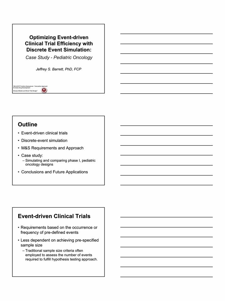
Optimizing Event Optimizing Event- driven driven Clinical Trial Efficiency with Clinical Trial Efficiency with Discrete Event Simulation: Discrete Event Simulation: Case Study - Pediatric Oncology Jeffrey S. Barrett, PhD, FCP Jeffrey S. Barrett, PhD, FCP 19th ACCP Frontiers Symposium: “Innovative Approach for Early Drug Development Disease Models and Novel Trial Design” Outline Outline Event Event- driven clinical trials driven clinical trials Discrete Discrete- event simulation event simulation M&S Requirements and Approach M&S Requirements and Approach Case study: Case study: Simulating and comparing phase I, pediatric Simulating and comparing phase I, pediatric oncology designs oncology designs Conclusions and Future Applications Conclusions and Future Applications Event Event- driven Clinical Trials driven Clinical Trials Requirements based on the occurrence or Requirements based on the occurrence or frequency of pre frequency of pre- defined events defined events Less dependent on achieving pre Less dependent on achieving pre- specified specified sample size sample size Traditional sample size criteria often Traditional sample size criteria often employed to assess the number of events employed to assess the number of events required to fulfill hypothesis testing approach. required to fulfill hypothesis testing approach.
Transcript

1

Optimizing EventOptimizing Event--driven driven Clinical Trial Efficiency with Clinical Trial Efficiency with Discrete Event Simulation:Discrete Event Simulation:Case Study - Pediatric Oncology

Jeffrey S. Barrett, PhD, FCPJeffrey S. Barrett, PhD, FCP

19th ACCP Frontiers Symposium: “Innovative Approach for Early Drug Development

Disease Models and Novel Trial Design”

OutlineOutline•• EventEvent--driven clinical trialsdriven clinical trials

•• DiscreteDiscrete--event simulationevent simulation

•• M&S Requirements and Approach M&S Requirements and Approach

•• Case study: Case study: –– Simulating and comparing phase I, pediatric Simulating and comparing phase I, pediatric

oncology designsoncology designs

•• Conclusions and Future ApplicationsConclusions and Future Applications

EventEvent--driven Clinical Trialsdriven Clinical Trials

•• Requirements based on the occurrence or Requirements based on the occurrence or frequency of prefrequency of pre--defined events defined events

•• Less dependent on achieving preLess dependent on achieving pre--specified specified sample size sample size –– Traditional sample size criteria often Traditional sample size criteria often

employed to assess the number of events employed to assess the number of events required to fulfill hypothesis testing approach.required to fulfill hypothesis testing approach.

2

EventEvent--driven Clinical Trialsdriven Clinical Trials

Screening Enrollment Evaluation Event

Patie

nt Q

ueue

Study Oversight / Monitoring / Analysis

EventEvent--driven Clinical Trialsdriven Clinical Trials

Wilcoxon rank sum; ITTWarning timeeDouble-blind, randomized, placebo-control trial•Darifenacin in OAB patients

General, linear model, random-effects analysis

Reaction time (w/ or w/o imaging)

Psychopharmacology, double-blind, placebo controlled fMRI

RRa; ITT b

RR; ITTRR; EFS d

MortalityComposite scorec

Survival

Randomized, parallel, active-control • OPTIMAAL Trial• BEAUTIFUL Trial• pancreatic cancer; best

supportive care vs glufosfamide

AnalysisEndpointsDesign / Examples

aRR = Response ratebITT = Intention- to- treatcMortality + hospital admissiondEFS = Event- free survivaleTime from first sensation of urgency to voiding

Copyright ©2005 American Academy of PediatricsMoya, F. R. et al. Pediatrics 2005;115:1018-1029

Enrollment flow diagram

EventEvent--driven Clinical Trialsdriven Clinical Trials“Therefore, the study was powered to test differences between these 2 products. Thehypothesis being tested was that “X” wouldbe superior to “Y”. A reference arm “Z” was of secondary interest. To keep the trial at a workable size, a 2:2:1 randomization scheme was used. The trial was designed to be event-driven, and the expected frequency of events was based on the observations reported in an earlier trialcomparing “X” and “Z”. Accordingly, weanticipated that the frequency of RDS would be 40% for X but only 30% for Y and the frequency of death related to RDS up to 14 days would be 7.5% for X but only 3.5% for Y. On the basis of these assumptions, the trial would continue until 420 infants had developed RDS and 66 infants had died from RDS-related causes. This number of events would provide 94% power to detect the prespecified difference between X and Y for the occurrence of RDS at 24 hours and 83% power for the occurrence of death related to RDS by 14 days.”

3

EventEvent--driven Clinical Trialsdriven Clinical TrialsWhat Drives Study Efficiency?What Drives Study Efficiency?

•• Time to enroll patientsTime to enroll patients

•• Patient Patient evaluabilityevaluability / replacement/ replacement

•• Time to Time to event(sevent(s) )

•• Waiting / decision / administrative time Waiting / decision / administrative time

Ultimately effects “n”Ultimately effects “n”

EventEvent--driven Clinical Trialsdriven Clinical TrialsSample size considerationSample size consideration

Simulating Time EventsSimulating Time EventsAdvantagesAdvantages

• Ability to compress time, expand time

• Ability to control sources of variation

• Avoids errors in measurement

• Ability to stop and review

• Ability to restore system state

• Facilitates replication• Modeler can control level of detail

*Discrete-Event Simulation: Modeling, Programming, and Analysis by G. Fishman, 2001, pp. 26- 27

4

*Simulation, Modeling & Analysis (3/e) by Law and Kelton, 2000, p. 4, Figure 1.1

Simulating Time EventsSimulating Time EventsApproachApproach

Discrete Event SimulationDiscrete Event Simulation• What is discrete- event simulation?

– Modeling, simulating, and analyzing systems– Computational and mathematical techniques

• Model: construct a conceptual framework that describes a system

• Simulate: perform experiments using computer implementation of the model

• Analyze: draw conclusions from output that assist in decision making process

• We will first focus on the model

Discrete Event SimulationDiscrete Event Simulation• Deterministic or Stochastic

– Does the model contain stochastic components?– Randomness is easy to add to a DES

• Static or Dynamic– Is time a significant variable?

• Continuous or Discrete– Does the system state evolve continuously or only at

discrete points in time?– Continuous: classical mechanics– Discrete: queuing, inventory, machine shop models

5

Discrete Event SimulationDiscrete Event SimulationDefinitionsDefinitions

• Discrete-Event Simulation Model– Stochastic: some variables are random– Dynamic: time progression is important– Discrete-Event: significant changes occur at

discrete time instancesvs

• Monte Carlo Simulation Model– Stochastic– Static: time evolution is not important

Discrete Event SimulationDiscrete Event SimulationModel TaxonomyModel Taxonomy

Discrete Event SimulationDiscrete Event SimulationComponentsComponents

• Activities where things happen to entities during some time (which may be governed by a probability distribution)

• Queues where entities wait an undetermined time

• Entities that wait in queues or get acted on in activities• Entities can have attributes like kind, weight, due date,

priority

6

- Patient arrivals, enrollment and evaluation, arrival queueing- Single site for incoming patients• IAT = Inter-arrival time (stochastic or constant)• IET = In-evaluability time (stochastic or constant)• EVT = Event time (stochastic)

State:• Now: current simulation time• Available: number of patients waiting to be enrolled• Enrolled: number of patients enrolled• Complete: number of patients evaluated (passed or reached endpoint)• Open: Boolean, true if study open to enrollmentEvents:• Pass: Patient completes evaluation without endpoint• IE: Patient is in-evaluable• Endpoint: Patient achieves endpoint

Discrete Event SimulationDiscrete Event SimulationClinical Trial Simulation Clinical Trial Simulation –– Simple ConstructSimple Construct

Arrival Event:Available := Available+1;If (Open)

Open:=TRUE;Schedule patient enrollmenti @ Now + IAT;

• IAT = Inter-arrival time• IET = In-evaluability time • EVT = Event time• Now: current simulation time• Available: number of patients waiting to be enrolled• Enrolled: number of patients enrolled• Complete: number of patients evaluated (passed or reached endpoint)• Open: Boolean, true if study open to enrollment

Patient arrives at site. If the study is open (and patient is available), they will be enrolled. Otherwise, the patient is skipped (enters another study).

Discrete Event SimulationDiscrete Event SimulationClinical Trial Simulation Clinical Trial Simulation –– Study level eventsStudy level events

Patient Enrolled:Available:=Available - 1;Enrolled:=Enrolled+1;If (Open:=TRUE) andif (Available>0)

Schedule patient enrollmenti+1 @ Now + IAT;Else

. . . criteria for halt or delay;

A patient enters the trial and gets evaluated

Discrete Event SimulationDiscrete Event SimulationClinical Trial Simulation Clinical Trial Simulation –– Patient level eventsPatient level events

7

Endpoint Event:Complete := Complete + 1;Patient event @ Now + IAT + EVT;. . . . Determine if endpoint reached count. . . . Determine if and how study proceeds

A patient reaches endpoint.

Discrete Event SimulationDiscrete Event SimulationClinical Trial Simulation Clinical Trial Simulation –– Patient level eventsPatient level events

Discrete Event SimulationDiscrete Event SimulationExecutionExecution

Time Event1 Enroll S11 Enroll S2

true

0

2

Patient 4

Now=

Patient 3

1

Time Event

2 Arrival S3

Now=2

Time Event7 Arrival S47 Enroll S4

1

2

4

Now=7

4 S2 Finish

Time Event

4 Enroll S3

3

Now=4

0

3

Time Event

10 S3 Finish

Now=10

0

1

Time Event

5 S1 Finish

Now=5

0

Simulation Time

Patient 1 Patient 2

Now=

2

false

Enrolled

StateVariables

Study Open

Available

0 1 3 4 5 6 7 8 9 10 11

0

0

IAT = 3EVT ≥ 4

Time Event0 Arrival S10 Arrival S2

Complete

2

Available Available

Enrolled Enrolled

Available

Enrolled

Complete Complete Available

Enrolled

Complete

• Time– Important to distinguish among simulation time, wallclock time, and

time in the physical system– Paced execution (e.g., immersive virtual environments) vs.

unpaced execution (e.g., simulations to analyze systems)

• DES computation: sequence of event computations– Modify state variables– Schedule new events

• DES System = model + simulation executive

Discrete Event SimulationDiscrete Event SimulationExecutionExecution

8

• Data structures– Pending event list to hold unprocessed events– State variables– Simulation time clock variable

• Program (Code)– Main event processing loop– Event procedures– Events processed in time stamp order

Discrete Event SimulationDiscrete Event SimulationExecutionExecution

Discrete Event SimulationDiscrete Event SimulationRealityReality

Case Study:Case Study:Pediatric Phase I Oncology TrialsPediatric Phase I Oncology Trials

• Decompose study and patient-level time-based events to explore time to event and time to complete

• Evaluate simulation models with respect to historical COG data

• Compare design efficiency for 3+3 versus Rolling 6 decision logic

9

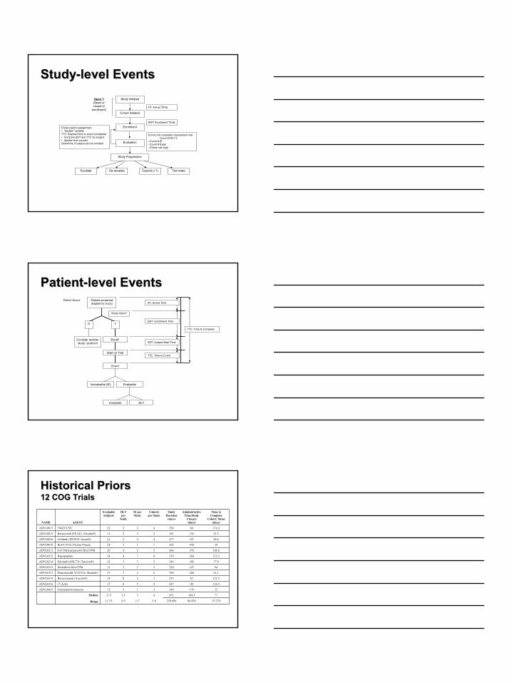
StudyStudy--level Eventslevel Events

Cohort Initiated

Enrollment

Study Progression

Escalate De-escalate TerminateExpand (+?)

Study Initiated

ENT: Enrollment Time

Enroll until completer requirement met–Count # DLT’s

–Count # IE–Count # Evals–Check rule logic

Evaluation

Check patient assignment • “Decide” variableTTC: Elapsed time to event (complete)• Compare ENT and TTC by subject• Update time counterDetermine if subject can be enrolled

AT: Arrival Time

Open ?(Open or closed to

enrollment)

PatientPatient--level Eventslevel EventsPatient screened(Eligible for study)

Study Open?

YN

Consider another study / protocol

Enroll*

Start on Trial

Event

EvaluableInevaluable (IE)

Complete DLT

AT: Arrival Time

ENT: Enrollment Time

SST: Subject Start Time

TTE: Time to Event

TTC: Time to Complete

Patient Queue

Historical PriorsHistorical Priors12 COG Trials12 COG Trials

33-27486-430220-6062-81-70-511-33Range

77184.5452432.521.5Median

5217828931513Oxaliplatin/IrinotecanADVL0415

116.51814274501717-AAGADVL0316

132.38723332014Bevacizumab (Avastin®)ADVL0314

61.120059682333Pemetrexed(LY231514; Alimta®)ADVL0311

9414722022211Decitabine/Dox/CPMADVL0215

77.618834453322Erlotinib (OSI-774; Tarceva®)ADVL0214

135.228453947424DepsipeptideADVL0212

106.637860655429G3139(Genesense®)/Dox/CPMADVL0211

5943056371328Hu14.18-IL2 Fusion ProteinADVL0018

88.634747744221Gefitinib (ZD1839; Iressa®)ADVL0016

95.315828123215Bortezomib (PS-341; Velcade®)ADVL0015

134.28652842222TMZ/CCNUADVL0011

Time to Complete

Cohort, Mean (days)

Administrative Time/Study

Closure (days)

Study Duration

(days)

Cohorts per Study

IE per Study

DLT per

Study

EvaluableSubjects

AGENTNAME

10

Representative study progression from COG phase I study (ADVL0311)

0 100 200 300 400 500 600 7000

5

10

15

20

25

30

35

# Subjects with DLTs# Inevaluable Subjects# Completers (Evalualble)# Cumulative Subjects Completed (Inevaluable + Evaluable)

1 2 3 4 5 6 7 8 9Cohort Progression

Elapsed Time (Days)

Num

ber o

f Sub

ject

s

Historical PriorsHistorical PriorsStudy ProgressionStudy Progression

Simulating Study Design EntitiesSimulating Study Design EntitiesDistributional AssumptionsDistributional Assumptions

N/ANormalTTC, Time to complete:Sum of ENT, SST and TTE‡

21, 28, 35 daysConstant, study constraint (typically 21 or 28 days)

TPASS, Time to evaluability (Pass):Days between start of evaluation and designation of patient as evaluable†

0.11, 0.25, 0.05Independent of dose cohort

P(IE), Probability of Inevaluability:Probability that a subject is inevaluable

Cohort start position varied 0, 1, or 2

.02 .05 .1 .3 .50 .75

.9 .95P(DLT), Probability of DLT:Cohorts (0 to 7)

Mean varied: 10, 15, 21 days

Normal, Mean = 21IET, Inevaluability Time:Days between start of evaluation and designation of patient as inevaluable

Uniform (Mean 20)Poisson (Mean 10, 15, 18 and 20 days)

Uniform; Mean = 20Poisson, Mean = 10, 15, 18, 20 days

TDLT, Time to DLT:Days between start of evaluation and the occurrence of DLT

Mean varied: 2, 5, 10 days

Normal, Mean = 2SST, Subject Start Time: Days between enrollment and start of evaluation

Mean Varied: 5, 20, 30, 40, 50, 100, 200 days; variance 1 – 3X

Poisson, Mean = 20ENT, Enrollment Time:Days between subject arrival or start of cohort for first subject* of cohort

Simulation Scenarios

Distribution and Assumptions

Parameter and Definition

* Can also reflect time between cohort being open to enrollment and actual arrival (enrollment) if study is suspended mid-cohort.† Assumes evaluable without DLT‡TTE (time to event) refers to the time in days that it takes for a subject to be designated as evaluable due to DLT (TDLT),

evaluable without DLT as a completer (TPASS) or inevaluable (IET)

Study Design ComparisonStudy Design ComparisonConventional 3+3 Conventional 3+3 vsvs “Rolling 6” Design“Rolling 6” Design

< 1/6 DLTs after de- escalation< 1/6 DLTs after de- escalationMaximal tolerated dose

After 6th patientAfter 3rd patientSuspension of trial

0/3 DLTs, or 1/6 after expansionOR

0/5, 0/6 DLTs if no expansion

0/3 DLTs, or 1/6 after expansionCriteria to escalate dose cohort

1/3 DLTs only if data from all prior subjects are available before subject 4 enrolls; otherwise continue to enroll patients 4, 5 and/or 6 until 1/N DLTs, then enroll to 6

1/3 DLTsCriteria to expand from 3 to 6 subjects

> 2 DLTs> 2 DLTsCriteria to de- escalate dose cohort

< 2 DLTs< 2 DLTsCriteria to take third subject

22No. subjects at start of trial

Rolling SixThree-Plus-ThreeCriteria

11

Design Performance Comparison

DES ApplicationDES Application• Simulate “N” Trials • Within each trial, populate “X” cohorts• Within each cohort, simulate “i” subjects for possible study enrollment• For each subject, simulate requisite event probabilities and time to event

based on random sample from target distributions• Determine actual event outcomes based on comparison of time to event

metrics (first event to occur is event of record)

Application of Design

Logic

StudyPopulationSimulation

• Enrollment status assessed based on study being “open”• Decision criteria assessed and counted• Enrollment procedure (# of subjects available for enrollment) assessed and

modified based on decision criteria• Cohort progression based on decision criteria (event counting) for cohort

and/or study being met• “Waiting time” added at various event milestones• Time to complete metrics (subjects, cohort, study) assessed

• Compare design proposals via event and time- based metrics• Chart / project study progression metrics

Design ChecksDesign ChecksStudy SimulationStudy Simulation

Deci de

20

40

60

TTC

Deci de

30

40

50

60

TTC

Deci de

30

40

50

60

TTC

ENT

10

20

30

40

TTE

ENT

10

20

30

TTE

ENT

10

20

30

40

TTE

Decide = 1 (DLT); Decide = 2 (IE); Decide = 3 (Pass)

• No correlation between TTE and ENT

• No correlation between TTC and decision (event outcome)

Table of cohort by DNAMEcohort DNAMEFrequency‚Percent ‚Row Pct ‚Col Pct ‚DLT-Eval‚Inevalua‚No DLT -‚ Total

‚uable ‚ble ‚ Eval ‚ƒƒƒƒƒƒƒƒƒˆƒƒƒƒƒƒƒƒˆƒƒƒƒƒƒƒƒˆƒƒƒƒƒƒƒƒˆ

1 ‚ 139 ‚ 800 ‚ 6561 ‚ 7500‚ 0.23 ‚ 1.33 ‚ 10.94 ‚ 12.50‚ 1.85 ‚ 10.67 ‚ 87.48 ‚‚ 0.55 ‚ 16.21 ‚ 22.12 ‚

ƒƒƒƒƒƒƒƒƒˆƒƒƒƒƒƒƒƒˆƒƒƒƒƒƒƒƒˆƒƒƒƒƒƒƒƒˆ2 ‚ 334 ‚ 803 ‚ 6363 ‚ 7500

‚ 0.56 ‚ 1.34 ‚ 10.61 ‚ 12.50‚ 4.45 ‚ 10.71 ‚ 84.84 ‚‚ 1.32 ‚ 16.27 ‚ 21.45 ‚

ƒƒƒƒƒƒƒƒƒˆƒƒƒƒƒƒƒƒˆƒƒƒƒƒƒƒƒˆƒƒƒƒƒƒƒƒˆ3 ‚ 684 ‚ 737 ‚ 6079 ‚ 7500

‚ 1.14 ‚ 1.23 ‚ 10.13 ‚ 12.50‚ 9.12 ‚ 9.83 ‚ 81.05 ‚‚ 2.69 ‚ 14.93 ‚ 20.49 ‚

ƒƒƒƒƒƒƒƒƒˆƒƒƒƒƒƒƒƒˆƒƒƒƒƒƒƒƒˆƒƒƒƒƒƒƒƒˆ4 ‚ 2130 ‚ 735 ‚ 4635 ‚ 7500

‚ 3.55 ‚ 1.23 ‚ 7.73 ‚ 12.50‚ 28.40 ‚ 9.80 ‚ 61.80 ‚‚ 8.39 ‚ 14.89 ‚ 15.62 ‚

ƒƒƒƒƒƒƒƒƒˆƒƒƒƒƒƒƒƒˆƒƒƒƒƒƒƒƒˆƒƒƒƒƒƒƒƒˆ5 ‚ 3604 ‚ 582 ‚ 3314 ‚ 7500

‚ 6.01 ‚ 0.97 ‚ 5.52 ‚ 12.50‚ 48.05 ‚ 7.76 ‚ 44.19 ‚‚ 14.19 ‚ 11.79 ‚ 11.17 ‚

ƒƒƒƒƒƒƒƒƒˆƒƒƒƒƒƒƒƒˆƒƒƒƒƒƒƒƒˆƒƒƒƒƒƒƒƒˆ6 ‚ 5315 ‚ 463 ‚ 1722 ‚ 7500

‚ 8.86 ‚ 0.77 ‚ 2.87 ‚ 12.50‚ 70.87 ‚ 6.17 ‚ 22.96 ‚‚ 20.93 ‚ 9.38 ‚ 5.80 ‚

ƒƒƒƒƒƒƒƒƒˆƒƒƒƒƒƒƒƒˆƒƒƒƒƒƒƒƒˆƒƒƒƒƒƒƒƒˆ7 ‚ 6409 ‚ 424 ‚ 667 ‚ 7500

‚ 10.68 ‚ 0.71 ‚ 1.11 ‚ 12.50‚ 85.45 ‚ 5.65 ‚ 8.89 ‚‚ 25.23 ‚ 8.59 ‚ 2.25 ‚

ƒƒƒƒƒƒƒƒƒˆƒƒƒƒƒƒƒƒˆƒƒƒƒƒƒƒƒˆƒƒƒƒƒƒƒƒˆ8 ‚ 6784 ‚ 392 ‚ 324 ‚ 7500

‚ 11.31 ‚ 0.65 ‚ 0.54 ‚ 12.50‚ 90.45 ‚ 5.23 ‚ 4.32 ‚‚ 26.71 ‚ 7.94 ‚ 1.09 ‚

ƒƒƒƒƒƒƒƒƒˆƒƒƒƒƒƒƒƒˆƒƒƒƒƒƒƒƒˆƒƒƒƒƒƒƒƒˆTotal 25399 4936 29665 60000

42.33 8.23 49.44 100.00Statistics for Table of cohort by DNAME

Statistic DF Value ProbƒƒƒƒƒƒƒƒƒƒƒƒƒƒƒƒƒƒƒƒƒƒƒƒƒƒƒƒƒƒƒƒƒƒƒƒƒƒƒƒƒƒƒƒƒƒƒƒƒƒƒƒƒƒChi-Square 14 29511.5039 <.0001Likelihood Ratio Chi-Square 14 35056.0231 <.0001Mantel-Haenszel Chi-Square 1 27795.9363 <.0001Phi Coefficient 0.7013Contingency Coefficient 0.5742Cramer's V 0.4959

Sample Size = 60000

Design ChecksDesign ChecksStudy SimulationStudy Simulation• Verification of distributional requirements

• By cohort composition

• Event-rate confirmation

5 10 15 20

TDLT

TDLT

0.75 3.45 6.15 8.85 11.55 14.25 16.95 19.65

TDLT

0

0.05

0.1

0.15

Density

0 10 20 30

ENT

ENT

0.0 3.2 6.4 9.6 12.8 16.0 19.2 22.4 25.6 28.8

ENT

0

0.1

0.2

0.3

Density

12

Design ChecksDesign ChecksStudy SimulationStudy Simulation

• The composite time scale

• TTC = ENT + SST + TTE

10 20 30 40 50

TTC

TTC

2.7 7.5 12.3 17.1 21.9 26.7 31.5 36.3 41.1 45.9

TTC

0

0.05

0.1

Density

Impact of sample size on DES study efficiency metrics with 3+3 decision rule*. Values reported as arithmetic mean (standard deviation)

2.14(0.85)

1.46(1.28)

3.10(1.10)

16.3(3.6)

530.6(124.4)

2000

2.15(0.81)

1.48(1.29)

3.09(1.05)

16.3(3.6)

537.7(128.5)

1000

2.23(0.86)

1.58(1.36)

3.08(1.03)

16.4(3.7)

543.7(131.9)

500

2.17(0.76)

1.39(1.22)

3.11(1.08)

16.4(3.2)

538.0(114.5)

200

2.23(0.76)

1.48(1.18)

3.14(1.04)

16.1(3.2)

528.0(115.8)

100

MTD Cohort(Cohort #)

IE/study(# subjects)

DLT/study(# subjects)

Subjects/study(# subjects)

Study Duration (Days)

Simulated Trials (#)

* Based model parameters used in simulation; P(DLT) = for cohorts 0 – 7, ENT = 20 days; IET = ; P(IE) = 0.11; TPASS = 21 days

Design ChecksDesign ChecksEffect of Simulation Sample SizeEffect of Simulation Sample Size

3+3 Design

N=100 N=200 N=500 N=1000 N=20000

100

200

300

400

500

600

700

800

900

1000

1100

1200

Number of Trial Simulations

Stud

y D

urat

ion

(Day

s)

R6 Design

N=100 N=200 N=500 N=1000 N=20000

100

200

300

400

500

600

700

800

900

1000

1100

Number of Trial Simulations

Stud

y D

urat

ion

(Day

s)

Design ChecksDesign ChecksEffect of Simulation Sample SizeEffect of Simulation Sample Size

13

3+3 Decision Rule

0 100 200 300 400 500 600 7000

5

10

15

20

25

30

35

# Subjects with DLTs# Inevaluable Subjects# Completers (Evalualble)# Cumulative Subjects Completed (Inevaluable + Evaluable)

Elapsed Time (Days)

Num

ber

of S

ubje

cts

R6 Decision Rule

0 100 200 300 400 5000

5

10

15

20

25

30

35

# Subjects with DLTs# Inevaluable Subjects# Completers (Evalualble)# Cumulative Subjects Completed (Inevaluable + Evaluable)

Elapsed Time (Days)

Num

ber

of S

ubje

cts

Post ProcessingPost ProcessingComparison of Study ProgressionComparison of Study Progression

Enrollment Time = 5 Days; Start at Cohort #2 (Increased p(DLT))

0 50 100 150 200 250 300 350 4000

10

20

30

40

Rolling 63+3

ELAPSED TIME

FREQ

UEN

CY

Post ProcessingPost ProcessingComparison of “Time to Complete”Comparison of “Time to Complete”

Enrollment Time = 5 Days; Start at Cohort #2 (Increased p(DLT))

0.0 2.5 5.0 7.5 10.00

5

10

15

20

25

30

35

40

45

Rolling 63+3

NUMBER OF DLTs

FREQ

UEN

CY

Post ProcessingPost ProcessingComparison of Number of Comparison of Number of DLTsDLTs / study/ study

14

Enrollment Time = 5 Days; Start at Cohort #2 (Increased p(DLT))

0 5 10 15 20 25 300

10

20

30

40

Rolling 63+3

NUMBER OF PATIENTS

Post ProcessingPost ProcessingComparison of Number of Patients / studyComparison of Number of Patients / study

ConclusionsConclusions• DES can be used to . . .

–Capture time-based study events–Evaluate time-based outcome

metrics–Compare design constructs–Evaluate decision rule logic

AcknowledgementsAcknowledgements

Jeffrey M Skolnik, MD

Peter C. Adamson, MD

Dimple Patel, MS

Bhuvana Jayaraman, BS

15

• Economic evaluation of tumor necrosis factor inhibitors for rheumatoid arthritis (Kamal, 2006)• Long-term costs and effects of new interventions in schizophrenia (Heeg, 2005)• Improving resource allocation / reducing the health burden related to schizophrenia (Haycox, 2005)• Cost analysis of a hospital-at-home service compared with conventional inpatient care (Campbell,

2001)

Pharmacoeconomics

• Impact of CV risk factor reduction on transplant outcome (McLean, 2005)• Impact of HIV on increasing the probability and the expected severity of tuberculosis outbreaks

(Porco, 2001)• Vaccine efficacy for susceptibility and infectiousness as prognostic factors for vaccine trials in HIV

(Longini, 1999)

Clinical Risk Factors

• CD4+ memory T cell generation to track individual lymphocytes over time (Zand, 2004)• Lymphocyte-mediated destruction of malignant lymphoid cells circulating through tissue

compartments of immune syngeneic C58 mice (Look, 1981)

Pharmacodynamics / Transduction Modeling

• Biology of end-stage liver disease and the health care organization of transplantation in the US (Shechter, 2005)

• Impact of surgical sequencing on post anesthesia care unit staffing (Marcon, 2005)• Cancellation of electively scheduled cases on the day of surgery (Dexter, 2005)• Performance of hospital accident and emergency department (Codrington-Virtue, 2005)• Staffing for entry screening, triage, medical evaluation, and drug dispensing stations in a

hypothetical antibiotic distribution center operating in disease prevalence bioterrorism response scenarios (Hupert, 2002)

Hospital Operations Research

• Methodological benefit of DES in depicting disease evolution of major depression (Le Lay, 2006)• Breast cancer incidence and mortality in the U.S. population from 1975 to 2000 (Fryback, 2006)• Patient progression following coronary event, through treatment pathways and subsequent events

(Cooper, 2002 and Babad, 2002)• Modeling of the AIDS pandemic - discrete-event simulation relating contact rate heterogeneity to

the rate of HIV spread (Leslie, 1990)

Disease Progression

ExamplesCategory

Discrete Event SimulationDiscrete Event SimulationExamplesExamples


Recommended