Fiscal rules and the sovereign default premium∗

Juan Carlos Hatchondo Leonardo Martinez Francisco Roch

Indiana U. IMF IMF

PRELIMINARY AND INCOMPLETE

Abstract

We study the effects of introducing fiscal rules—understood as constraints on the decision-making ability of current and future governments—using a model of sovereign default. Wefirst calibrate the benchmark model without a fiscal rule using as a reference economiesthat pay a significant sovereign default premium. We then study the effects of introducingdifferent sequences of limits to (i) the debt level, (ii) changes in the debt level, and (iii) themaximum sovereign premium the government can pay when it issues debt. We show thatoptimal debt limits vary greatly across parameterizations of the model. In contrast, optimalsovereign-premium limits are very similar across parameterizations. Given the uncertaintyabout model parameter values and political constraints that may force common fiscal ruletargets across economies, these findings imply that sovereign premium targets are preferableover debt targets. In addition, we show that (i) rules allow the government to implementa less procyclical fiscal policy but should not necessarily promote a countercyclical fiscalpolicy; (ii) intermediate targets are important when rules are introduced; (iii) introducingrules can result in reductions of the levels of debt and sovereign default premium withoutany fiscal adjustment (and even with fiscal expansions); and (iv) benefits from imposing arule arise even if the government is not shortsighted, and may be substantial.

JEL classification: F34, F41.Keywords: Fiscal Rules, Debt Ceiling, Spread Target, Fiscal Consolidation, Default,

Sovereign Default Premium, Debt Exchange, Countercyclical Policy, Endogenous BorrowingConstraints, Long-term Debt, Debt Dilution.

∗For comments and suggestions, we thank Gaston Gelos, Jorge Roldos, and seminar participants at the 2012Sovereign Debt Workshop at the Federal Reserve Bank of Richmond, the 2011 European Economic Association andEconometric Society Meeting, and the IMF Institute and Strategy, Policy, and Review departments. Remainingmistakes are our own. The views expressed herein are those of the authors and should not be attributed to theIMF, its Executive Board, or its management.E-mails: juanc.hatchondo@gmail.com; leo14627@gmail.com; froch@imf.org.

1

1 Introduction

This paper studies the optimality of fiscal rules and measures their effects using a baseline

sovereign default framework. Fiscal rules are restrictions imposed (often in laws or in the consti-

tution) to the future governments’ ability to conduct fiscal policy. We abstract from fiscal rules

enforcement issues and focus on the effects that a fiscal rule would have if the government could

commit to enforce it. Some countries have mitigated enforcement limitations, for instance, by

granting constitutional status to their fiscal rules. For example, Germany (in 2009) and Spain (in

2011) amended their constitutions to introduce fiscal rules. The super-majorities, referendums,

or waiting periods typically required to amend a constitution limit the discretionary power of

policymakers in office. In addition fiscal rules are being complemented with formal enforcement

procedures (for instance, automatic correction mechanisms such as “sequestration” processes,

and automatic sanctioning procedures), and independent fiscal bodies that set budget assump-

tions and monitor the implementation of fiscal rules (Budina et al., 2012; IMF, 2009; Schaechter

et al., 2012). Several empirical studies find that well design fiscal rules are associated with

stronger fiscal performance (Corbacho and Schwartz, 2007; Debrun and Kumar, 2007; Debrun

et al., 2008; Deroose et al., 2006; EC, 2006; Kopits, 2004).

A consensus has emerged among policymakers about the desirability of fiscal rules targeting

low sovereign debt levels that help deter fiscal crises and facilitate implementing more counter-

cyclical fiscal policies.1 Nevertheless, significant uncertainty remains about the optimal value of

fiscal rules’ targets.

More generally, while sovereign debt levels are often at the center of policy debates, these

debates are rarely guided by economic theory. For example, the IMF flagship fiscal publication

has recently stated that “the optimal-debt concept has remained at a fairly abstract level, whereas

the safe-debt concept has focused largely on empirical applications” (IMF, 2013a). Similarly, the

IMF chief economist asked: “what levels of public debt should countries aim for? Are old rules

1For instance, in an IMF Staff Position Note, Blanchard et al. (2010) argue that “A key lesson from the crisisis the desirability of fiscal space to run larger fiscal deficits when needed.” They also note that “Medium-termfiscal frameworks, credible commitments to reducing debt-to-GDP ratios, and fiscal rules (with escape clauses forrecessions) can all help in this regard.” Discussions about the overhaul of the fiscal rules in the Eurozone provideother examples of this view.

2

of thumb, such as trying to keep the debt to GDP ratio below 60 percent in advanced countries,

still reliable?” (Blanchard, 2011).

This paper intends to shed light on the optimal value of fiscal rules’ targets and to quantify the

effects of introducing optimal fiscal rules. To that end, we study a model of strategic sovereign

default a la Eaton and Gersovitz (1981). This framework is commonly used for quantitative

studies of sovereign debt and has been shown to generate a plausible behavior of sovereign debt

and spread —i.e., the difference between the sovereign bond yield and the risk-free interest rate.2

We first focus on fiscal rules imposing a sovereign debt limit. We find that the government

benefits from such rules. This happens because rules imposing debt limits allow the government

to commit to lower future debt levels, mitigating the overborrowing implied by the debt dilution

problem (Hatchondo et al., 2010b): the government would like to commit to future debt levels

that imply low sovereign risk.3

We find that the optimal debt limit vary greatly across parameterizations of the model. In

particular, a limit that is optimal (and produces welfare gains) for one parameterization may

produce welfare losses for others. This should not be surprising in the light of the well know

sovereign debt intolerance problem: the relationship between sovereign debt levels and sovereign

risk varies greatly across countries (Reinhart et al., 2003). This indicates that debt levels coun-

tries would want to commit to (those that imply low sovereign risk) may vary greatly across

countries. Figure 1 illustrates the debt intolerance problem using Latin American countries. On

the one extreme, the average sovereign spread in Brazil was below 200 basis points in 2012 for a

debt level above 60 percent of its GDP. On the other extreme, the average sovereign spread in

Ecuador was above 800 basis points for a debt level below 20 percent of its GDP. The figure also

show significant changes in the levels of sovereign debt and spreads over time.

The findings above present two important challenges. First, they indicate that given the

2See, for instance, Aguiar and Gopinath (2006), Arellano (2008), Benjamin and Wright (2008), Boz (2011),Lizarazo (2005, 2006), and Yue (2010). These models share blueprints with the models used in studies of householdbankruptcy—see, for example, Athreya et al. (2007), Chatterjee et al. (2007), Li and Sarte (2006), Livshits et al.(2008), and Sanchez (2010). For models of non-strategic defaults see Bi (2011) and Bi and Leeper (2012).

3There is debt dilution in our framework because we assume long-term debt. Chatterjee and Eyigungor (2012)and Hatchondo and Martinez (2009) show that long-term debt is essential for accounting for interest rate dynamicsin a framework with sovereign defaults.

3

Argentina

Brazil Chile

Ecuador

Mexico Peru Uruguay

Venezuela

Bolivia 2012

0

200

400

600

800

1000

1200

1400

1600

1800

2000

0 10 20 30 40 50 60 70

EM

BIG

Sp

rea

ds

(b

asi

s p

oin

ts)

General government gross debt/GDP

Figure 1: Sovereign debt and spreads in Latin America countries.

uncertainty about model parameter values, a default model a la Eaton and Gersovitz (1981) may

not be useful to identify optimal fiscal rule debt targets. Quantitative studies using this model

topically pin down the relationship between the levels of sovereign debt and risk for the economy

under study by making the long-run average levels of sovereign debt and spreads calibration

targets. But in many cases, it is not even clear which target to choose. For instance, this is

evident for European Economies currently facing sovereign risk: the introduction of the euro

seem to have had significant temporary effects on sovereign debt and spread dynamics making

difficult to infer the future long-run levels of these variables from past data. The levels of both

sovereign debt and spread display a U-shape, bottoming out before the crisis (for example,

the sovereign spread for Spain was around zero between 1999 and 2007, and even negative in

some periods). As illustrated in Figure 1, significant changes in sovereign debt and spreads

are also common outside Europe. Thus, it would be difficult for policymakers to take seriously

4

predictions about optimal sovereign debt levels that come out of this model, perpetuating the

disconnect between theoretical and practical discussions about sovereign debt levels discussed by

IMF (2013a).

The second challenge implied by our findings come from political constraints that may force

common fiscal rule targets across economies. Perhaps the best known example are the common

sovereign debt limits imposed by the Maastricht Treaty. Our results indicate that, in light of

the well known debt intolerance problem, optimal sovereign debt limits may vary greatly across

countries. Common sovereign debt levels are also used across countries by the IMF, for instance,

as one of the criteria to decide the level of scrutiny in surveillance (IMF, 2013b; IMF, 2013c).

We then focus on fiscal rules imposing a limit to the maximum sovereign premium the govern-

ment can pay when it issues debt. We find that, in contrast with debt limits, optimal sovereign-

premium limits are very similar across parameterizations. This is not surprising. As explained

above, gains from imposing fiscal rules arise because rules achieve a reduction in sovereign risk.

Debt limits achieve this reduction indirectly. Thus, a debt limit that is too loose may fail to

achieve the desired risk reduction. And a debt limit that is too tight may unnecessarily prevent

a government from borrowing, producing welfare losses. In contrast, limits to the sovereign pre-

mium attack directly the debt dilution problem. Our findings suggest that sovereign premium

targets should be preferable over debt targets both to give robust recommendations to a single

country and to provide common targets across countries. While sovereign debt levels dominate

policy debates, the role of sovereign spreads seems to be increasing. For instance, Claessens

et al. (2012) argue that “the challenge is to complement fiscal rules affecting quantities most

productively with market-based mechanisms using price signals.” In addition, recent revisions of

the IMF fiscal stainability framework incorporate sovereign spreads as an additional criteria to

guide the level of scrutiny in surveillance (IMF, 2013b). Should we ask what levels of sovereign

spread should countries aim for, instead of asking what levels of public debt should countries

aim for? Our findings suggest that we should.

We also study other key element of discussions on fiscal rules. We find that (i) rules allow

the government to implement a less procyclical fiscal policy but should not necessarily promote

a countercyclical fiscal policy; (ii) intermediate targets are important when rules are introduced;

5

(iii) introducing rules can result in reductions of the levels of debt and sovereign default premium

without any fiscal adjustment (and even with fiscal expansions); and (iv) benefits from imposing

a rule arise even if the government is not shortsighted, and may be substantial.

1.1 Related Literature

In spite of the great interest among policymakers, theoretical studies on fiscal rules are relatively

scarce. Several theoretical studies focus on the desirability of a balanced-budget rule for the

U.S. federal government (see Azzimonti et al., 2010 and the references therein). Garcia et al.

(2011) compare a balanced budget rule with a structural surplus rule. Beetsma and Uhlig

(1999) show how by imposing lower debt levels, the Stability and Growth Pact may help control

inflation in the European Monetary Union. Beetsma and Debrun (2007) discuss how additional

flexibility in the Stability and Growth Pact may improve welfare. Pappa and Vassilatos (2007)

and Poplawski Ribeiro et al. (2008) find that debt ceilings may be preferable over constraints on

the government’s deficit. Medina and Soto (2007) use a model of the Chilean economy to show

that a structural balanced fiscal rule mitigates the macroeconomic effects of copper-price shocks.

The studies mentioned in the previous paragraph do not discuss the robustness of spread and

debt targets, which is the main focus of our analysis. Furthermore, these studies abstract from

the effect that the expectation about future indebtedness has on the default premium, which is

the key for the gains of imposing fiscal rules in our environment. In these studies, rules may

be beneficial because of a conflict of interest between the government and private agents (for

instance, because the government is myopic or because of political polarization), or because of a

conflict of interest among governments of different countries (for instance, in a monetary union).

In contrast, we study a model with benevolent governments but in which there is a conflict

between current and future governments. We show that benefits from imposing a rule arise even

if the government is not shortsighted. We also discuss how assuming shortsighted government

would change the results.

Our findings also relate to those presented by Calvo (1988), who also discuses gains from

introducing interest-rate ceilings for sovereign debt. However, there are important differences

6

between the two analyses. In Calvo’s (1988) model, an interest-rate ceiling is used to eliminate

bad equilibria in a multiple-equilibria framework. In contrast, we study a framework in which

the equilibrium without a fiscal rule is always bad (as reflected in high default risk) and show

that a fiscal rule can improve the equilibrium. In our framework, gains from the fiscal rule

appear because of time-inconsistency problem that arises when one models long-term debt (debt

dilution), and not because of multiple equilibria.

Several empirical studies analyze the relationship between fiscal rules and fiscal policy (Poterba,

1996, reviews the literature for U.S. states; Debrun et al. (2008), present evidence for Europe),

and between fiscal rules and the government’s financing costs (Eichengreen and Bayoumi, 1994;

Heinemann et al., 2011; Iara and Wolff, 2011; Lowry and Alt, 2001; and Poterba and Rueben,

1999). However, difficulties in identifying the effects of fiscal rules are well documented (Poterba,

1996; Heinemann et al., 2011). We measure these effects through the lens of a default model.

When comparing predictions in this paper with past experiences with fiscal rules, one should

keep in mind that we are assuming that the government can commit to enforcing a rule while

this is not necessarily the case in reality.

An extensive literature discusses the importance of sovereign debt dilution (see Hatchondo

et al., 2010b, and the references therein). Within this literature, Chatterjee and Eyigungor

(2013) and Hatchondo et al. (2010b) present the studies that are closer to this paper. As we

do, they study the quantitative effects of remedies to the dilution problem. While we focus on

fiscal rules, the instruments countries are using to deal with sovereign debt problems (Budina

et al., 2012; IMF, 2009; Schaechter et al., 2012), Chatterjee and Eyigungor (2013) and Hatchondo

et al. (2010b) discuss the effects of introducing improvements to sovereign debt contracts. Chat-

terjee and Eyigungor (2013) study the effects of introducing a seniority structure. Hatchondo

et al. (2010b) study the effects of introducing debt covenants that penalize future borrowing.

This makes the remedies for debt dilution proposed by Chatterjee and Eyigungor (2013) and

Hatchondo et al. (2010b) fundamentally different to the one studied in this paper: since fiscal

rules impose a debt reduction, we must present a careful analysis of transitions and the speed

of fiscal adjustments, which Chatterjee and Eyigungor (2013) and Hatchondo et al. (2010b) left

mostly unexplored. We find that introducing rules can result in reductions of the levels of debt

7

and sovereign default premium without any fiscal adjustment (and even with fiscal expansions).

The relationship between fiscal adjustment and debt levels is at the center of current policy

debates (IMF, 2012). We contribute to the discussions of this relationship. We also show that

announcing intermediate targets is important when rules are introduced. While countries rec-

ognize that time is needed to achieve the debt reductions implied by fiscal rules, intermediate

targets Arab not always part of the design of fiscal rules.4

The paper also contributes to the discussion of the optimal cyclicality of fiscal policy. Cuadra

et al. (2010) show that in the sovereign default model without a fiscal rule, it is optimal for the

government to borrow less when income is low. Thus, the optimal fiscal policy is procyclical.5 We

show that as the fiscal rule reduces sovereign risk, the optimal policy becomes less procyclical.

However, as long as default risk is significant, the government prefers a fiscal rule that implies a

procyclical fiscal policy. Such rule achieves a larger reduction of default risk at the expense of a

higher consumption volatility. Only among fiscal rules for which default risk is insignificant, the

government would prefer a countercyclical fiscal policy.

The exercises presented in this paper also illustrate how a sovereign default framework a la

Eaton and Gersovitz (1981) can be used to evaluate fiscal consolidation programs and the implied

sovereign debt dynamics. An alternative approach is to use the debt stainability framework

(Adler and Sosa, 2013; Ghosh et al., 2011; Tanner and Samake, 2006) commonly used for policy

analysis (see, for instance, IMF, 2013c, and IMF Article IV country reports). Our analysis

complements the stainability analysis by presenting endogenous sovereign spreads (that, for

example, capture the effects of expectation of future adjustments), endogenous borrowing policies

(that react to fiscal rules), and welfare criteria to discuss optimal policy.

The rest of the article proceeds as follows. Section 2 shows the role of fiscal rules in a three-

period model. Section 3 presents the infinite horizon model. Section 4 discusses the calibration.

Section 5 presents the results. Section 6 concludes.

4For instance, Germany amended its constitution in 2009 to introduce a fiscal rule to be enforced after 2016for the federal government and after 2020 for regional governments. Similarly, Spain amended its constitution in2011 to introduce a fiscal rule to be enforced after 2020.

5This is consistent with the observed fiscal policy in emerging economies, as documented by Gavin and Perotti(1997), Ilzetzki et al. (2012), Kaminsky et al. (2004), Talvi and Vegh (2009), and Vegh and Vuletin (2011).

8

2 Three-period model

The economy lasts for three periods t = 1, 2, 3. The government receives a sequence of endow-

ments given by y1 = 0, y2 = 0, and y3 > 0. The only uncertainty in the model is about the value

of y3. The government is benevolent and makes its decision on a sequential basis. The govern-

ment acting in period j maximizes E

[

∑3t=j u (ct)

]

, where E denotes the expectation operator,

ct represents period-t consumption in the economy, and the utility function u is increasing and

concave.

The government can borrow to finance consumption in periods 1 and 2. A bond issued in

period 1 promises to pay one unit of the good in period 2 and (1− δ) units in period 3. Thus, if

δ = 1, the government issues one-period bonds in period 1. If δ < 1, we say that the government

issues long-term bonds in period 1. A bond issued in period 2 promises to pay one unit of the

good in period 3.

The government may choose to default in period 3.6 If the government defaults, it does

not pay its debt but looses a fraction φ of the period-3 endowment y3. Bonds are priced by

competitive risk-neutral investors who discount future payments at a rate of 1.

Let bt denote the number of bonds issued by the government and qt denote the price at which

the government sells bonds in period t . The budget constraints are:

c1 = −b1q1(b1, b2),

c2 = −b2q2(b1, b2)− b1,

c3 = y3(1− dφ)− (1− d)[b1(1− δ) + b2],

where d denotes the government’s default decision and is equal to 1 if the government defaults

and is equal to 0 otherwise.

2.1 Results

In this setup, it is optimal to borrow because borrowing enables the government to smooth out

consumption over time. However, borrowing decisions are restricted by the limited commitment

6In period 2 there is no uncertainty and, therefore, there cannot be a meaningful default decision.

9

problem faced by the government.

The equilibrium default decision is given by

d(b1, b2, y3) =

1 if y3 <b1(1−δ)+b2

φ,

0 otherwise..

Given the above defaulting rule, the price of a bond issued in period 1 is given by

q1(b1, b2) = 1 + (1− δ)P

[

y3 <b1(1− δ) + b2

φ

]

, (1)

where P denote the probability function. The price of a bond issued in period 2 is given by

q2(b1, b2) = P

[

y3 <b1(1− δ) + b2

φ

]

.

Given that the government does not borrow in period 3, there is no role for rules that limit

the government behavior in that period. It is easy to verify that there is also no role for rules in

period 1. Such rules would only restrict the choice set available to the government. Proposition

1 shows that when the government can only issue one-period debt, there is also no role for fiscal

rules in period 2

Proposition 1 Suppose δ = 1, i.e., bonds issued in period 1 pay off in period 2 alone. Then,

the government’s period-1 expected utility cannot be improved with a fiscal rule that limits debt

choices in period-2.

Proof: The government’s period-1 expected utility is maximized by b∗1 and b∗2 such that

u′ (c∗1) = u′ (c∗2) =E

[

u′ (c∗3)(

1− d(b∗1, b∗2, y3)

)]

q2(b∗1, b∗2) + b∗2

δq2(b∗1 ,b∗

2)

δb2

,

where

c∗1 = b∗1q1(b∗1, b

∗2),

c∗2 = b∗2q2(b∗1, b

∗2)− b∗1,

c∗3 = y3(1− dφ)− (1− d)[b∗1(1− δ) + b∗2],

10

The government’s period-2 optimal choice satisfies

u′ (c2) =E

[

u′ (c3)(

1− d(b1, b2, y3))]

q2(b1, b2) + b2δq2(b1,b2)

δb2

.

Therefore, if the government chooses b∗1 in period 1, it expects that the government acting in

period 2 will choose b∗2. Thus, the government’s period-1 expected utility cannot be improved with

a period-2 debt limit (fiscal rule).

Proposition 2 shows that a role for fiscal rules arises when the government issues long-term

debt (in period 1).

Proposition 2 Suppose δ < 1, i.e., the government issues long-term debt in period 1. Then, a

period-2 fiscal rule is necessary to maximize the government’s period-1 expected utility.

Proof: The government’s period-1 expected utility is maximized by b∗1 and b∗2 such that

u′ (c∗1)

[

q1(b∗1, b

∗2) + b∗1

δq1(b∗1, b

∗2)

δb1

]

= u′ (c∗2)

[

1− b∗2δq2(b

∗1, b

∗2)

δb1

]

+(1−δ)E[

u′ (c∗3)(

1− d(b∗1, b∗2, y3)

)]

,

u′ (c∗2)

[

q2(b∗1, b

∗2) + b∗2

δq2(b∗1, b

∗2)

δb2

]

= E

[

u′ (c∗3)(

1− d(b∗1, b∗2, y3)

)]

− u′ (c∗1) b∗1

δq1(b∗1, b

∗2)

δb2. (2)

The government’s period-2 optimal choice satisfies

u′ (c2)

[

q2(b1, b2) + b2δq2(b1, b2)

δb2

]

= E

[

u′ (c3)(

1− d(b1, b2, y3))]

. (3)

Thus, since equation (3) is different from (2), the allocation that maximizes the government’s

period-1 expected utility cannot be attained without a fiscal rule (if the period-1 government

chooses b∗1, the period-2 government will not choose b∗2).

In contrast, the allocation that maximizes the government’s period-1 expected utility can triv-

ially be attained with a fiscal rule that forces the period-2 government to choose b∗2 (with the

period-1 government choosing b∗1).7

7Note that the allocation that maximizes the government’s period-1 expected utility could be attained with a

debt limit b2 ≤ b∗2 or a limit to the price at which the government can sell debt q2(b∗

1, b∗

2) as both these limits will

make the period-2 government choose b∗2.

11

The role for a fiscal rule arises because the rule eliminates the debt dilution problem. With

long-term debt, period-2 debt issuances dilute the price of period-1 debt (equation 1). The

allocation that maximizes the government’s period-1 expected utility recognizes that the price

of the debt issued in period 1 is negatively affected by debt issuances in period 2 (last term of

the right-hand side of equation 2). But this is not a cost for the government acting in period-2

(equation 3) and, consequently, leads to overborrowing in period-2 in the absence of a fiscal rule.

Summing up, this section illustrated how while there is no role for fiscal rules with one-period

debt (proposition 1), a fiscal rule is necessary to implement the optimal allocation with long-term

debt. This is important because the case with long-term debt is the empirically relevant case.

We next study a richer model that allows us to quantify gains from introducing fiscal rules and

draw lessons for the design of fiscal rules.

3 Infinite horizon model

There is a single tradable good. The economy receives a stochastic endowment stream of this

good yt, where

log(yt) = (1− ρ)µ+ ρ log(yt−1) + εt,

with |ρ| < 1, and εt ∼ N (0, σ2ǫ ).

The government’s objective is to maximize the present expected discounted value of future

utility flows of the representative agent in the economy, namely

Et

∞∑

j=t

βj−tu (cj) ,

where E denotes the expectation operator, β denotes the subjective discount factor, and the

utility function is assumed to display a constant coefficient of relative risk aversion denoted by

γ. That is,

u (c) =c1−γ − 1

1− γ.

As in Hatchondo and Martinez (2009) and Arellano and Ramanarayanan (2010), we assume

that a bond issued in period t promises an infinite stream of coupons, which decreases at a

12

constant rate δ. In particular, a bond issued in period t promises to pay one unit of the good in

period t + 1 and (1− δ)s−1 units in period t + s, with s ≥ 2.

Each period, the government makes two decisions. First, it decides whether to default.

Second, it chooses the number of bonds that it purchases or issues in the current period.

As previous studies of sovereign default, we assume that the recovery rate for debt in default—

i.e., the fraction of the loan lenders recover after a default—is zero and that the cost of defaulting

is not a function of the size of the default. The second assumption implies that, as in Arellano and

Ramanarayanan (2010), Chatterjee and Eyigungor (2012) and Hatchondo and Martinez (2009),

when the government defaults, it does so on all current and future debt obligations. This is

consistent with the behavior of defaulting governments in reality. Sovereign debt contracts often

contain an acceleration clause and a cross-default clause. The first clause allows creditors to

call the debt they hold in case the government defaults on a payment. The cross-default clause

states that a default on any government obligation also constitutes a default on the contracts

containing that clause. These clauses imply that after a default event, future debt obligations

become current.

There are two costs of defaulting in the model. First, a defaulting sovereign is excluded from

capital markets. Once excluded, the country regains access to capital markets with probability

ψ ∈ [0, 1].8 Second, if a country has defaulted on its debt, it faces an income loss of φ (y) in

every period in which it is excluded from capital markets. Following Chatterjee and Eyigungor

(2012), we assume a quadratic loss function φ (y) = max{0, d0y + d1y2}.

Following Arellano and Ramanarayanan (2010), we assume that the price of sovereign bonds

satisfies a no arbitrage condition with stochastic discount factor M(y′, y) = exp(−r − αε′ −

0.5α2σ2ǫ ), where r denotes the risk-free rate at which lenders can borrow or lend. This allows us

to introduce a risk premium. Several studies document that the risk premium is an important

component of sovereign spreads and that a significant fraction of the spread volatility in the data

is accounted for by the volatility in the risk premium (Borri and Verdelhan, 2009; Broner et al.,

2007; Longstaff et al., 2011; Gonzalez-Rozada and Levy Yeyati, 2008).

8Hatchondo et al. (2007) solve a baseline model of sovereign default with and without the exclusion cost andshow that eliminating this cost affects significantly only the debt level generated by the model.

13

The model of the discount factor we use is a special case of the discrete-time version of the

Vasicek one-factor model of the term structure (Vasicek, 1977; Backus et al., 1998). With this

formulation, the risk premium is determined by the income shock in the borrowing economy. It

may be more natural to assume that the lenders’ valuation of future payments is not perfectly

correlated with the sovereign’s income. However, the advantage of our formulation is that it

avoids introducing additional state variables to the model. In this paper, benefits from intro-

ducing fiscal rules result from the mitigation of the debt dilution problem. Hatchondo et al.

(2010b) show that the effects of debt dilution on default risk are robust to assuming that there

is a shock to the cost of borrowing that is not perfectly correlated with the sovereign’s income,

and to assuming that lenders are risk neutral.

We focus on Markov Perfect Equilibrium. That is, we assume that in each period, the

government’s equilibrium default and borrowing strategies depend only on payoff-relevant state

variables. As discussed by Krusell and Smith (2003), there may be multiple Markov perfect

equilibria in infinite-horizon economies. In order to avoid this problem, we solve for the equi-

librium of the finite-horizon version of our economy, and we increase the number of periods of

the finite-horizon economy until value functions and bond prices for the first and second periods

of this economy are sufficiently close. We then use the first-period equilibrium functions as an

approximation of the infinite-horizon-economy equilibrium functions.

3.1 Recursive formulation of the no-rule benchmark

We first present the recursive formulation for the benchmark economy, in which there is no fiscal

rule. Let b denote the number of outstanding coupon claims at the beginning of the current

period, and b′ denote the number of outstanding coupon claims at the beginning of the next

period. Let d denote the current-period default decision. We assume that d is equal to 1 if the

government defaulted in the current period and is equal to 0 if it did not. Let V denote the

government’s value function at the beginning of a period, that is, before the default decision is

made. Let V0 denote the value function of a sovereign not in default. Let V1 denote the value

function of a sovereign in default. Let F denote the conditional cumulative distribution function

14

of the next-period endowment y′. For any bond price function q, the function V satisfies the

following functional equation:

V (b, y) = maxdǫ{0,1}

{dV1(y) + (1− d)V0(b, y)}, (4)

where

V1(y) = u (y − φ (y)) + β

∫

[ψV (0, y′) + (1− ψ) V1(y′)]F (dy′ | y) , (5)

and

V0(b, y) = maxb′≥0

{

u (y − b+ q(b′, y) [b′ − (1− δ)b]) + β

∫

V (b′, y′)F (dy′ | y)

}

. (6)

The bond price is given by the following functional equation:

q(b′, y) =

∫

M(y′, y) [1− h (b′, y′)]F (dy′ | y)

+ (1− δ)

∫

M(y′, y) [1− h (b′, y′)] q(g(b′, y′), y′)F (dy′ | y) , (7)

where h and g denote the future default and borrowing rules that lenders expect the government

to follow. The default rule h is equal to 1 if the government defaults, and is equal to 0 otherwise.

The function g determines the number of coupons that will mature next period. The first term in

the right-hand side of equation (7) equals the expected value of the next-period coupon payment

promised in a bond. The second term in the right-hand side of equation (7) equals the expected

value of all other future coupon payments, which is summarized by the expected price at which

the bond could be sold next period.9

Equations (4)-(7) illustrate that the government finds its optimal current default and bor-

rowing decisions taking as given its future default and borrowing decision rules h and g. In

equilibrium, the optimal default and borrowing rules that solve problems (4) and (6) must be

equal to h and g for all possible values of the state variables.

Definition 3 A Markov Perfect Equilibrium is characterized by

1. a set of value functions V , V1, and V0

9Assuming risk-neutral lenders, Chatterjee and Eyigungor (2012) demonstrate that an equilibrium bond pricefunction exist and is decreasing with respect to the debt level.

15

2. a default rule h and a borrowing rule g,

3. a bond price function q,

such that:

(a) given h and g, V , V1, and V0 satisfy functional equations (4), (5), and (6), when the

government can trade bonds at q;

(b) given h and g, the bond price function q is given by equation (7); and

(c) the default rule h and borrowing rule g solve the dynamic programming problem defined

by equations (4) and (6) when the government can trade bonds at q.

3.2 Fiscal rules

We introduce fiscal rules by imposing into the framework presented above sequences of limits

to (i) the debt level, (ii) changes in the debt level, and (iii) the maximum sovereign premium

the government can pay when it issues debt. Thus, when the rule (i.e., the sequence of limits)

is announced, the government’s maximization problem is not recursive until the limits stops

changing over time. We solve the problem backwards from the first period in which it becomes

recursive.

Thus, when the rule (i.e., the sequence of debt ceilings) is announced, the government’s

maximization problem is not recursive until the debt ceiling stops changing with t. We solve the

problem backwards from the first period in which it becomes recursive.

3.3 Fiscal policy

Fiscal policy is very stylized in sovereign default frameworks a la Eaton and Gersovitz (1981).

The government may tax private agents in order to service its debt or may give transfers to

private agents using resources it borrows. Each period, the government chooses the (possibly

16

negative) level of tax revenues τ . When the country is in default, τ = 0 and private agents

consume all available resources (c = y − φ(y)). When the country is not in default, private

agents pay taxes (c = y − τ) and the government uses tax revenues to service debt that is not

rolled over, i.e., τ = b− q (b′, y) [b′ − (1− δ)b].

4 Calibration

As Hatchondo et al. (2010a), we solve the model numerically using value function iteration

and interpolation.10 We present a benchmark calibration targeting features of the data (as

previous studies, we use data from Argentina before the 2001 default) and, in order to check the

robustness of fiscal rules, we also study alternative parameterizations (that still produce plausible

implications).

Table 1 presents the benchmark calibration. We assume that the representative agent in the

sovereign economy has a coefficient of relative risk aversion of 2, which is within the range of

accepted values in studies of business cycles. A period in the model refers to a quarter. The

risk-free interest rate is set equal to 1 percent. As in Hatchondo et al. (2009), parameter values

that govern the endowment process are chosen so as to mimic the behavior of GDP in Argentina

from the fourth quarter of 1993 to the third quarter of 2001. The parametrization of the income

process is similar to the parametrization used in other studies that consider a longer sample

period (Aguiar and Gopinath, 2006). As in Arellano (2008), we assume that the probability of

regaining access to capital markets (ψ) is 0.282.

With δ = 0.0341, bonds have an average duration of 4.19 years in the simulations of the

baseline model.11 Cruces et al. (2002) report that the average duration of Argentinean bonds

included in the EMBI index was 4.13 years in 2000. This duration is not significantly different

10We use linear interpolation for endowment levels and spline interpolation for asset positions. The algorithmfinds two value functions, V1 and V0. Convergence in the equilibrium price function q is also assured.

11We use the Macaulay definition of duration, which with the coupon structure assumed in this paper is givenby

D =1 + r∗

δ + r∗,

where r∗ denotes the constant per-period yield delivered by the bond.

17

Sovereign’s risk aversion γ 2

Interest rate r 0.01

Income autocorrelation coefficient ρ 0.9

Standard deviation of innovations σǫ 0.027

Mean log income µ (-1/2)σ2ǫ

Exclusion ψ 0.282

Duration δ 0.0341

Discount factor β 0.961

Default cost d0 -0.69

Default cost d1 1.017

Risk premium α 3

Table 1: Parameter values.

from what is observed in other emerging economies. Using a sample of 27 emerging economies,

Cruces et al. (2002) find an average duration of 4.77 years, with a standard deviation of 1.52.

We calibrate the discount factor, the income cost of defaulting (two parameter values), and

the lenders’ risk premium parameter to target four moments: A mean spread of 7.4 percent, a

standard deviation of the spread of 2.5 percent, a mean public external debt to (annual) GDP

ratio of 40 percent in the pre-default samples of our simulations (the exact definition of these

samples is presented in Section 4.1), and a default frequency of three defaults per 100 years. The

first three targets are computed using Argentine data from 1993 to 2001. Even though it is not

obvious which value for the default frequency one should target, we include the default frequency

as a target in our calibration because it has received considerable attention in the literature, it

is clearly influenced by lenders’ risk premium parameter, and it influences the welfare gains from

the imposition of fiscal rules. We target a frequency of three defaults per 100 years because this

frequency is often used in previous studies (Arellano, 2008; Aguiar and Gopinath, 2006).12

12Hatchondo et al. (2010b) show that the effects of debt dilution are similar in model economies with three

18

We also present results for three alternative parameterizations that use all parameter values

in the benchmark except for: (i) ψ = 0.24, (ii) ψ = 0.19, (iii) ψ = 0.15 and α = 0. Lowering

ψ—the probability of regaining access to capital markets after defaulting—increases the cost of

defaulting and thus increases the sovereign spread for a given debt level. This allows us to study

model economies with different levels of debt tolerance. The values we assume for ψ are between

the range estimated and assumed in the literature (Dias and Richmond, 2007; Mendoza and Yue,

2012). The third alternative parameterization also assume that lenders are risk neutral. This

is the most common assumption in the sovereign default literature. Thus, studying this case

facilitates comparing our results with those in previous studies and allows us to show that gains

from imposing fiscal rules are robust to changes in the lenders risk aversion.

5 Results

First, we show that simulations of the model produce plausible implications, including a procycli-

cal fiscal policy. Second, we show that the government can benefit from committing to a fiscal

rule that establishes a debt limit. Third, we show that imposing the debt limit that is optima

for the benchmark calibration may produce welfare losses in other economies. Fourth, we shows

that imposing a spread limit for debt issuances produces welfare gains comparable to the ones

obtained with debt limits. However, in contrast to the optimal debt limit for the benchmark

economy, the optimal spread limit for the benchmark economy still produces welfare gains in

other economies. Fifth, we discuss whether fiscal rules should allow for larger fiscal deficits in

bad times. Sixth, we discuss the cost of restricting the government to choose among fiscal rules

that do not establish intermediate fiscal adjustment targets. Seventh, we show that the benefits

from imposing fiscal rules are even larger when we assume that the government benefits from

debt holders capital gains, or that the government is shortsighted.

and six defaults per 100 years. The discount factor value we obtain is relatively low but higher than the onesassumed in previous studies (Aguiar and Gopinath, 2006, assume β = 0.8). Low discount factors may be a resultof political polarization in emerging economies (Amador, 2003; Cuadra and Sapriza, 2008).

19

Argentina 94-01 Benchmark ψ = 0.24 ψ = 0.19 ψ = 0.15, α = 0

E(Rs) 7.44 7.42 6.83 6.09 4.99

σ (Rs) 2.51 2.52 2.34 2.1 1.89

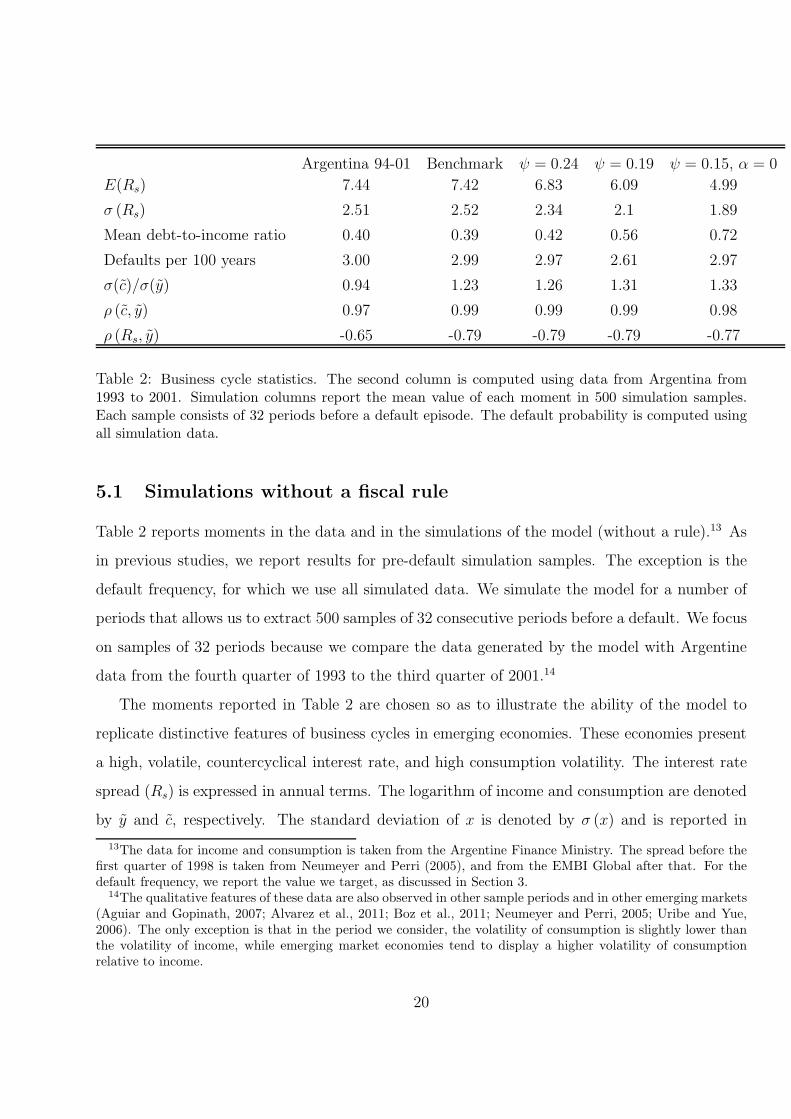
Mean debt-to-income ratio 0.40 0.39 0.42 0.56 0.72

Defaults per 100 years 3.00 2.99 2.97 2.61 2.97

σ(c)/σ(y) 0.94 1.23 1.26 1.31 1.33

ρ (c, y) 0.97 0.99 0.99 0.99 0.98

ρ (Rs, y) -0.65 -0.79 -0.79 -0.79 -0.77

Table 2: Business cycle statistics. The second column is computed using data from Argentina from1993 to 2001. Simulation columns report the mean value of each moment in 500 simulation samples.Each sample consists of 32 periods before a default episode. The default probability is computed usingall simulation data.

5.1 Simulations without a fiscal rule

Table 2 reports moments in the data and in the simulations of the model (without a rule).13 As

in previous studies, we report results for pre-default simulation samples. The exception is the

default frequency, for which we use all simulated data. We simulate the model for a number of

periods that allows us to extract 500 samples of 32 consecutive periods before a default. We focus

on samples of 32 periods because we compare the data generated by the model with Argentine

data from the fourth quarter of 1993 to the third quarter of 2001.14

The moments reported in Table 2 are chosen so as to illustrate the ability of the model to

replicate distinctive features of business cycles in emerging economies. These economies present

a high, volatile, countercyclical interest rate, and high consumption volatility. The interest rate

spread (Rs) is expressed in annual terms. The logarithm of income and consumption are denoted

by y and c, respectively. The standard deviation of x is denoted by σ (x) and is reported in

13The data for income and consumption is taken from the Argentine Finance Ministry. The spread before thefirst quarter of 1998 is taken from Neumeyer and Perri (2005), and from the EMBI Global after that. For thedefault frequency, we report the value we target, as discussed in Section 3.

14The qualitative features of these data are also observed in other sample periods and in other emerging markets(Aguiar and Gopinath, 2007; Alvarez et al., 2011; Boz et al., 2011; Neumeyer and Perri, 2005; Uribe and Yue,2006). The only exception is that in the period we consider, the volatility of consumption is slightly lower thanthe volatility of income, while emerging market economies tend to display a higher volatility of consumptionrelative to income.

20

percentage terms. The coefficient of correlation between x and z is denoted by ρ (x, z). Moments

are computed using detrended series. Trends are computed using the Hodrick-Prescott filter with

a smoothing parameter of 1, 600. Table 2 also reports the mean debt-to-income ratio, where the

debt is calculated as b/(δ + r).

Table 2 shows that the baseline model matches the data reasonably well. As in the data, in the

simulations of the baseline model consumption and income are highly correlated and the spread

is countercyclical. Consumption volatility is higher than income volatility, which is consistent

with the findings in Neumeyer and Perri (2005) and Aguiar and Gopinath (2007). The model

also matches well the moments we targeted.

Table 2 also shows that as expected, as we decrease the probability of regaining access to

credit markets after defaulting, model simulations are characterized by more debt tolerance.

That is, they are characterized by higher debt and lower spreads. Similarly, when we assume

risk-neutral lenders, borrowing becomes more attractive, and simulations feature higher debt and

lower spread. In addition, Table 2 shows that the assumed lenders risk aversion does not play a

significant role in the model’s ability to replicate key features of the data.

5.2 Procyclical fiscal policy without a fiscal rule

Figure 2 shows that fiscal policy is procyclical without a fiscal rule: Taxes tend to be higher (or

transfers tend to be lower) when income is lower. This is consistent with the findings presented by

Cuadra et al. (2010), who show that fiscal policy is procyclical in a sovereign default framework

with a richer model of fiscal policy. The intuition for the procyclicality of fiscal policy is the

following: In bad times (when income is low), the cost of borrowing is relatively high and the

government chooses to finance more of its debt service obligations with taxes instead of new

issuances.

5.3 Debt limits

For simplicity, we first focus on the debt limit to be imposed in no-rule economies without initial

debt and with the trend level of income. In this Subsection, we also focus in constant debt

21

0.8 0.9 1 1.1 1.2 1.3−0.07

−0.06

−0.05

−0.04

−0.03

−0.02

−0.01

0

0.01

Output

Gov

ernm

ent T

rans

fers

/ O

utpu

t

Figure 2: Income and government transfers in the simulations of the benchmark economy.

ceilings that do not depend on the income level.

Table 3 shows that welfare gains are maximized with a debt ceiling of 25 percent of trend

income. We measure welfare gains as the constant proportional change in consumption that

would leave domestic consumers indifferent between continuing living in the benchmark economy

(without a fiscal rule) and moving to an economy with a fiscal rule. Let V B and V R denote the

value functions in the benchmark economy and an economy with a fiscal rule, respectively. The

welfare gain of moving from the benchmark economy to an economy with a fiscal rule is given by

(

V R(b, y)

V B(b, y)

)1

1−γ

− 1.

The government benefits from implementing a fiscal rule because the rule mitigates the debt

dilution problem. Figure 3 illustrates how imposing a debt limit creates new borrowing oppor-

tunities for the government. On the one hand, a debt ceiling limits the amount the government

can borrow today. On the other hand, the ceiling also limits future borrowing, enabling the

government to pay a lower interest rate for any current borrowing level. The figure also shows

that the sharp reduction in spreads implied by the debt limit allows the government to lower

its debt level significantly with a relatively mild reduction in its borrowing: while with the 20

percent ceiling implies a debt reduction of 18 percent of trend annual income, it only implies a

22

No limit 35% 30% 25% 20%

Defaults per 100 years 2.99 2.86 1.33 0.42 0.09

E (Rs) 7.42 6.64 3.6 1.66 0.54

σ (Rs) 2.52 2.85 1.93 1.29 0.7

σ (c) /σ (y) 1.23 1.12 1.08 1.05 1.02

Welfare gains 0.00 0.04 0.38 0.55 0.37

Table 3: Simulation results for different debt limits.

reduction in loan values of about 5 percent of trend annual income.

Table 3 also shows how lower debt levels implied by the imposition of a debt limit attenuates

the procyclicality of fiscal policy, as reflected in a lower volatility of consumption. By reducing

default risk, debt limits reduce both the mean spread and the responsiveness of the spread to

income shocks, which is reflected in a lower standard deviation of the spread. These findings

support the consensus among policymakers about the desirability of targeting low sovereign debt

levels to create room for the implementation of countercyclical fiscal policy (Blanchard et al.,

2010).

5.4 Robustness of debt limits

In this subsection we investigate wether optimal debt limit for one economy can still produce

benefits when imposed to a different economy. This issue is important because political con-

straints may lead to supranational fiscal rules that imposed common debt limits across countries

as happened, for instance, with the Maastricht Treaty. Furthermore, since there is uncertainty

about parameter values, one would like policy recommendations that come out of the model to

be robust to changes of these values.

Table 4 shows that the 25 percent debt limit that maximizes welfare in the benchmark may

produce substantial welfare losses in other model economies. Intuitively, the 25 percent debt

limit would be too tight for an economy with a higher debt tolerance. Thus, while the results

in Subsection 5.3 illustrate the potential benefits from imposing debt limits, this subsection

23

0 0.1 0.2 0.3 0.4 0.50

1

2

3

4

5

6

7

8

9

10

Next period debt / Mean annual output

An

nu

al

Sp

read

No Rule

Rule 20

0 0.1 0.2 0.3 0.4 0.5 0.60

0.05

0.1

0.15

0.2

0.25

Next period debt / Mean annual output

q(b

’,y)*

b’ /

Mean

an

nu

al

ou

tpu

t

No Rule

Rule 20

Figure 3: Government’s borrowing opportunities with and without a debt ceiling. The left panelpresents the menu of end-of-period debt (−b′/4(δ + r)) and spread the government can choose from.The right panel presents the amount a government without debt could borrow as a function of isend-of-period debt.

24

Benchmark ψ = 0.24 ψ = 0.19 ψ = 0.15, α = 0

Defaults per 100 years 0.42 0.09 0.01 na

E (Rs) 1.66 0.53 0.13 na

σ (Rs) 1.29 0.69 0.20 na

σ (c) /σ (y) 1.05 1.03 1.02 na

Welfare gains 0.55 0.44 -0.03 -0.96

Table 4: Economies with a 25 percent debt limit. The economy with ψ = 0.15 and α = 0 does notfeature defaults (therefore, we cannot report results for pre-default samples).

illustrates the potential risks of doing so.

5.5 Spread limit

In this subsection we study the effects of imposing fiscal rules banning the government from

borrowing when the spread it would have to pay is higher than a spread limit. Table 5 shows that

imposing such spread limit produces welfare gains comparable to the ones implied by imposing

a debt limit. The difference between the welfare gain obtained with the optimal debt and

spread limits can be accounted for by the difference in the implied cyclicality of fiscal policy.

Comparing Tables 3 and 5 shows that when compared with debt limits, spread limits achieve a

larger reduction in default risk with a given reduction in debt levels. For instance, the 1 percent

spread limit reduces the default frequency to 0.66 (per 100 years) with a mean debt level of

0.32, while a 30 percent debt limit only reduces the default frequency to 1.33. Spread limits

achieve this by imposing a more procyclical fiscal policy, as reflected in the higher consumption

volatility. Differences between the cyclicality of fiscal policy implied by debt and spread limits

could be corrected by allowing these limits to depend on the current income level. Subsection

5.7 discusses the optimal cyclicality of fiscal policy implied by fiscal rules. We find that the main

difference between debt and spread limits is in their robustness, which we discuss next.

25

No target 3% 2% 1.5% 1% 0.5%

Mean debt-to-income ratio 0.39 0.37 0.35 0.33 0.32 0.29

Defaults per 100 years 2.99 1.76 1.22 0.91 0.66 0.34

E (Rs) 7.42 3.4 2.4 1.85 1.33 0.74

σ (Rs) 2.51 1.07 0.90 0.80 0.69 0.53

σ (c) /σ (y) 1.23 1.71 1.73 1.72 1.70 1.65

Welfare gains 0.00 0.51 0.64 0.68 0.72 0.70

Table 5: Simulation results for different spread limits.

5.6 Robustness of spread limits

Table 6 shows that the spread limit for the benchmark economy still produces substantial welfare

gains when imposed to a different economy. Thus, comparing Tables 4 and 6 shows a crucial

difference between fiscal rules targeting debt and spread levels. While the optimal debt limit for

one economy is likely to produce welfare losses in other economies, the optimal spread limit for

one economy still produces substantial welfare gains in other economies. That spread targets

are more robust than debt limits is intuitive. Recall that gains from imposing fiscal rules arise

because rules allow the government to pay a lower spread. Spread targets achieve this directly

independently from the economy’s debt intolerance. In contrast, optimal debt limits are highly

dependent on the economy’s debt intolerance. The government benefits from higher debt levels

as long as these levels do not imply higher sovereign risk. Table 6 shows that spread limits

naturally allow for higher debt levels in economies with more debt tolerance.

Again, this difference between fiscal rules targeting debt and spread levels is important be-

cause of both political constraints that lead to common fiscal rules for different economies, and

uncertainty about the parameter values of models used to guide to choice of optimal targets

for fiscal rules. The remainder of the paper abstract from robustness issues and focus on the

benchmark calibration.

26

Benchmark ψ = 0.24 ψ = 0.19 ψ = 0.15, α = 0

Mean debt-to-income ratio 0.32 0.47 0.50 0.68

Defaults per 100 years 0.66 0.64 0.66 0.89

E (Rs) 1.33 1.21 1.28 1.17

σ (Rs) 0.69 0.57 0.65 0.47

σ (c) /σ (y) 1.70 1.94 1.80 2.16

Welfare gains 0.72 0.80 0.94 0.94

Table 6: Economies with a 1 percent spread limit.

5.7 Fiscal rules and the cyclicality of fiscal policy

We next discuss whether fiscal rules should allow for a larger government deficit in bad times,

and whether this would promote a more countercyclical fiscal policy. This is a central element of

discussions about fiscal rules in policy circles. In particular, our analysis allows us to shed light

on the desirability of “escape clauses” that soften fiscal rules during recessionary periods. These

clauses are present in many fiscal rules (Budina et al., 2012; IMF, 2009; Schaechter et al., 2012).

Our findings serve as a warning against promoting these clauses in the presence of sovereign risk.

It should be mentioned that one may see our analysis of the cyclicality of fiscal policy as

limited because in our model, fiscal policy does not play a role in stabilizing aggregate income

(we study an stochastic exchange economy). However, evidence of negligible or even negative

fiscal multipliers for highly indebted countries (Ilzetzki et al., 2012) reinforces our result about

the optimality of fiscal rules promoting procyclical fiscal policy in the presence of significant

default risk. Nevertheless, it should also be mentioned that estimates of fiscal multipliers range

from significant positive numbers to also significant but negative numbers (IMF, 2012). Our

contribution is to discuss these issues emphasizing the role of sovereign risk while abstracting

from the controversial role of fiscal policy in stabilizing aggregate income.

As in previous subsections, for simplicity, we focus on an economy that initially is not indebted

and has a current income level equal to the trend. This allows us to reduce the number of rules

27

we have to look at. Searching for optimal fiscal rules for indebted economies would also require

to search for optimal transition paths, which we do in the following subsections.

We focus on rules imposing debt limits. Since the sovereign spread is a function of income,

focusing on debt limits instead of on spread limits facilitates the discussion of how the limit

imposed by the rule is allowed to change with income. We assume the government can commit

to a debt limit that is a liner function of the current income:

b¯(y) = a0 + a1y. (8)

We search for the optimal coefficients of rules like the ones specified in equation (8).15

We find that the optimal rule is procyclical and imposes a limit on the debt-to-income ratio

of 25 percent of annualized income (a1 = 1 and a0 = 0). Figure 4 shows that this rule implies a

welfare gain equivalent to a permanent consumption increase of 0.63 percent.

−2 −1.5 −1 −0.5 0 0.5 1 1.5 20.25

0.3

0.35

0.4

0.45

0.5

0.55

0.6

0.65

0.7

Slope coefficient of debt rule

Wel

fare

gai

n (%

of c

ons.

)

y = mean − std. dev.y = meany = mean + std. dev.

Figure 4: Welfare gain from implementing rules with an average debt ceiling of 25 percent of meanannual income and different slope coefficients.

15However, we still do not allow the government to issue income-indexed debt (Hatchondo and Martinez, 2012).The overwhelming majority of sovereign debt bonds are not GDP-indexed in part because of verifiability andmoral hazard issues that are not present in our stylized model. One may think that these issues could also makeit difficult to establish contingent fiscal rule targets. Nevertheless, contingent targets are common in fiscal rules.These targets are often implemented with the assistance of independent fiscal bodies (Budina et al., 2012; IMF,2009; Schaechter et al., 2012).

28

Slope coefficient of debt ceiling rule - 2 -1 -0.5 0 0.5 1 2

Defaults per 100 years 0.79 0.75 0.67 0.42 0.23 0.12 0.03

E (Rs) 2.63 2.41 2.13 1.66 1.07 0.68 0.10

σ (Rs) 1.47 1.41 1.43 1.05 0.85 0.55 0.03

σ (c) /σ (y) 1.05 1.04 0.98 1.05 1.25 1.48 1.82

Table 7: Simulation results with a debt ceiling b¯(y) = a0 + a1y, for different values of a1, and values of

a0 such that the average ceiling is equivalent to 25 percent of mean annual income.

Table 7 presents business cycle statistics from simulations of economies with rules that imply

an average ceiling of 25 percent of mean income. The table shows that the preferred rule priori-

tizes lowering the default probability over reducing private consumption volatility: It leads to a

frequency of 0.12 defaults every hundred years (instead of 3 in the no-rule benchmark and 0.42

with the acyclical ceiling) and to a standard deviation of consumption that is 48 percent higher

than the standard deviation of income (instead of 23 percent higher in the no-rule benchmark

and 5 percent higher with the acyclical ceiling).

Table 7 shows that if instead of choosing an acyclical ceiling (a1 = 0), the government

chooses countercyclical ceilings (a1 < 0) that allow for higher debt levels in periods of lower in-

come, there are no significant changes in consumption volatility. During low-income periods, the

default probability becomes more sensitive to changes in debt levels. Therefore, a countercyclical

ceiling that allows for more debt in those periods loosens the government’s commitment to lower

future default probabilities. This contributes to increase the level and countercyclicality of the

government’s borrowing cost, making it more difficult to conduct countercyclical fiscal policy.

The government prefers a countercyclical ceiling only when debt levels implied by the rule is low

enough that it eliminates default risk and, consequently, the countercyclicality of the borrowing

cost.

29

5.8 Debt limits for indebted economies without intermediate targets

In contrast with previous subsections, the remainder of the paper discusses fiscal rules for in-

debted economies. In order to lower the number of rules we have to study, we restrict attention

to rules imposing limits that do not depend on the current income level.

This subsection assumes that when the government introduces a fiscal rule, it makes two

announcements: (i) a debt limit, and (ii) the period in which this debt limit is going to start being

imposed. We search for the government optimal announcements. Note that we are assuming

the government cannot choose intermediate debt limits. As mentioned before, it is often the

case that government introduce fiscal rules without intermediate targets. We discuss the role of

intermediate debt limit targets in Subsection 5.9.

We consider three pre-rule states characterized by a debt level of 38 percent of mean income

and by different income levels, which determine the level of the sovereign spread. The relatively

low-risk state has a spread of 5.1 percent, the normal-risk state has a spread of 7.4 percent, and

the high-risk state with has spread of 15 percent.

Table 8 presents the optimal fiscal rule for each of the three states described above. The

table shows that the level of pre-rule default risk does not significantly affect the rule to which

the government would like to commit. Welfare is maximized with a debt ceiling of 30 percent of

mean income and a delay of four years between the rule announcement period and the period in

which the ceiling starts being enforced.

Announcement-period spread (pre announcement) 5.1% 7.4% 15.0%

Optimal transition length (quarters) 18 17 17

Optimal debt ceiling after the transition (% of trend annual income) 30% 30% 30%

Announcement-period spread (post announcement) 4.2% 6.0% 14.7%

Long-run average spread 3.6% 3.6% 3.6%

Welfare gain 0.23% 0.23% 0.22%

Table 8: Optimal rules without intermediate targets for pre-rule states with different sovereign spreads.The debt level is constant across pre-rule states (38 percent of mean income) but income levels differ.

30

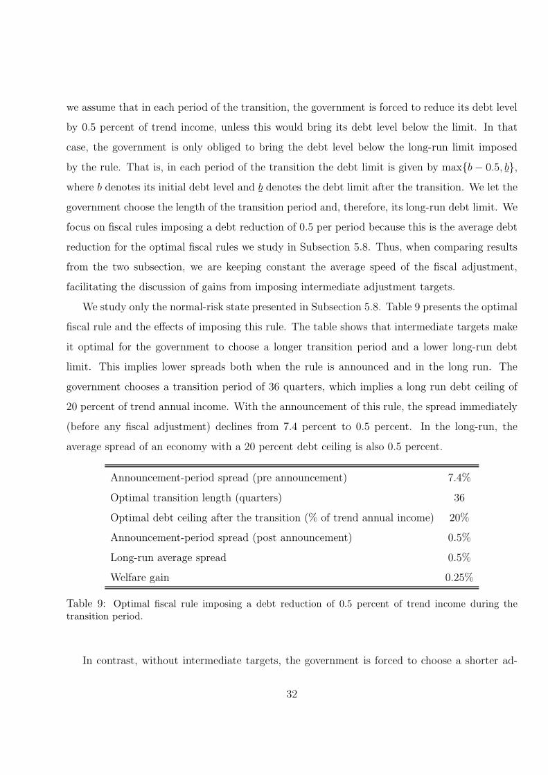
Figure 5 presents the mean debt and spread levels after the the optimal rule announcement for

transition paths in which the government does not default. Figure 5 shows that the government

chooses to do the bulk of the debt reduction during the last year of the four years transition

period. During the first three years, the government benefits from lower spreads without reducing

its debt level more than what it would have reduced it without a rule.

0 0.5 1 1.5 2 2.5 3 3.5 4 4.529

30

31

32

33

34

35

36

37

38

39

40

Years after the rule announcement

Deb

t−to

−in

com

e ra

tio

Pre−rule spread = 5.1% & rulePre−rule spread = 7.4% & rulePre−rule spread = 15% & rulePre−rule spread = 5.1% & no rulePre−rule spread = 7.4% & no rulePre−rule spread = 15% & no rule

0 0.5 1 1.5 2 2.5 3 3.5 4 4.50

2

4

6

8

10

12

14

16

18

Years after the rule announcement

Anu

al s

prea

d (in

%)

Pre−rule spread = 5.1% & rulePre−rule spread = 7.4% & rulePre−rule spread = 15% & rulePre−rule spread = 5.1% & no rulePre−rule spread = 7.4% & no rulePre−rule spread = 15% & no rule

Figure 5: Mean debt-to-income ratio (−b′/(δ+r)4y ) and interest rate spread during transitions that follow

the announcement of the optimal rule, for samples without defaults.

Figure 5 also shows that after the rule announcement, the spread is expected to decline

faster when the pre-rule spread is higher. This explains why welfare gains from implementing

the optimal rule are similar for the three cases consider in Table 8, in spite of a much lower

announcement-period spread decline in the case with a 15 percent pre-rule spread.

5.9 Debt limits for indebted economies with intermediate targets

This subsection illustrates the importance of intermediate targets for fiscal rules (and, more

generally, for fiscal adjustment programs). As in subsection 5.8, in this subsection we focus on

fiscal rules that impose a transition period and a constant debt limit after the transition period.

However, in this subsection we focus on rules that impose a debt reduction in every period

during the transition (in contrast with the fiscal rules studied in Subsection 5.8). In particular,

31

we assume that in each period of the transition, the government is forced to reduce its debt level

by 0.5 percent of trend income, unless this would bring its debt level below the limit. In that

case, the government is only obliged to bring the debt level below the long-run limit imposed

by the rule. That is, in each period of the transition the debt limit is given by max{b− 0.5, b¯},

where b denotes its initial debt level and b¯denotes the debt limit after the transition. We let the

government choose the length of the transition period and, therefore, its long-run debt limit. We

focus on fiscal rules imposing a debt reduction of 0.5 per period because this is the average debt

reduction for the optimal fiscal rules we study in Subsection 5.8. Thus, when comparing results

from the two subsection, we are keeping constant the average speed of the fiscal adjustment,

facilitating the discussion of gains from imposing intermediate adjustment targets.

We study only the normal-risk state presented in Subsection 5.8. Table 9 presents the optimal

fiscal rule and the effects of imposing this rule. The table shows that intermediate targets make

it optimal for the government to choose a longer transition period and a lower long-run debt

limit. This implies lower spreads both when the rule is announced and in the long run. The

government chooses a transition period of 36 quarters, which implies a long run debt ceiling of

20 percent of trend annual income. With the announcement of this rule, the spread immediately

(before any fiscal adjustment) declines from 7.4 percent to 0.5 percent. In the long-run, the

average spread of an economy with a 20 percent debt ceiling is also 0.5 percent.

Announcement-period spread (pre announcement) 7.4%

Optimal transition length (quarters) 36

Optimal debt ceiling after the transition (% of trend annual income) 20%

Announcement-period spread (post announcement) 0.5%

Long-run average spread 0.5%

Welfare gain 0.25%

Table 9: Optimal fiscal rule imposing a debt reduction of 0.5 percent of trend income during thetransition period.

In contrast, without intermediate targets, the government is forced to choose a shorter ad-

32

justment periods because it knows that fiscal adjustments will be delayed (Figure 5). Since the

government has a tendency of delaying fiscal adjustments, choosing a long adjustment period

would imply that the adjustment would start far in the future and, therefore, would be heavily

discounted by lenders. Consequently, it is optimal for the government to choose shorter tran-

sition periods when the rule does not establish intermediate targets. Since the government is

restricted to a shorter transition period, it is optimal to choose a more moderate adjustment.

Comparing Tables 8 and 9 shows that the possibility of designing a fiscal rule that lowers

default risk may depend crucially on whether the rule specifies intermediate targets for debt

reduction. While announcing the optimal rule with intermediate targets lowers the sovereign

spread by 6.9 percent, announcing the optimal rule without intermediate targets only lower the

sovereign spread by 1.4 percent. Thus, our results are a warning against the common practice of

announcing fiscal rules without intermediate targets.

5.10 Spread limits for indebted economies without intermediate tar-

gets

We next show that introducing fiscal rules that impose spread limits may also produce welfare

gains for indebted economies. We focus on the normal-risk state introduced in Subsection 5.8—a

debt level of 38 percent of trend annual income and an income level that implies a spread of

7.4 percent (the mean spread in our benchmark simulations). In this Subsection, we search for

the optimal spread limit to be imposed immediately. In contrast with imposing a debt limit

immediately, imposing a spread limit immediately allows for a gradual debt reduction. We find

that the optimal spread target is 2 percent. Imposing this target produces a welfare gain of 0.32

percent. With the announcement of the imposition of the optimal target, the spread falls from

7.4 percent to 2.8 percent. Thus, compared with the effects of introducing a debt limit (without

intermediate targets) presented in Table 8, introducing a spread limit results in a much larger

reduction in sovereign risk (4.6 percent instead of 1.4 percent) and a larger welfare gain (0.32

percent instead of 0.23 percent).

The optimal spread target for an indebted economy is higher than the one we found for an

33

economy without debt in Subsection 5.5. For an indebted economy, choosing a lower spread

target implies a longer period without debt issuances and, therefore, a longer period without

gaining from the improved borrowing conditions implied by the target. This cost is not present

for economies without debt. In next subsection, we show that the government would be better

off with a sequence of spread targets that eventually impose a lower target.

5.11 Spread limits for indebted economies with intermediate targets

We now study fiscal rules that impose a sequence of spread targets. We search for the optimal

sequence of spread targets imposing the following restrictions: (i) the sequence ends with a

constant spread target, and (ii) between the periods in which the first and last targets are

introduced, the difference between the minimum price at which the government can sell a bond

in the current and previous periods is equal to 3 percent of the price of a risk-free bond. Thus,

the government can choose: (i) the final spread target, and (ii) the duration of the adjustment

of the spread targets (and, therefore, the initial spread target). As in the previous subsections,

we focus on the normal-risk state.

We find that the optimal sequence of spread targets starts with a target of 4.2 percent in the

period in which the rule is introduced, with the target declining to its 1.5 percent final value

over 38 quarters (with an average target decline of 29 basis points per year). The initial target

of 4.2 percent allows the government to borrow (and thus benefit from the improvement of the

borrowing terms) since the quarter in which the target is introduced, in which the target is

binding. The welfare gain from imposing the sequence of targets is 0.36 percent.

Figure 6 illustrates how fiscal rules may reduce sovereign debt and risk even with a minimum

fiscal sacrifice, as represented by a decline in consumption (over the consumption that would have

occurred without a rule). In fact, it is possible to implement fiscal rules that lower sovereign debt

and risk without any fiscal sacrifice. The figure presents the evolution of expected consumption

after introducing the optimal spread limit rule with intermediate targets. It shows that after the

quarter in which the rule is introduced, consumption is expected to be higher with the rule in

34

every period.

0.93

0.94

0.95

0.96

0.97

0.98

0.99

0 1 2 3 4 5 6 7 8

Co

nsu

mp

tio

n

Years after the fiscal rule announcement

Without the rule

With the rule

Figure 6: Consumption as a percentage of income after the imposition of a fiscal rule.

Figure 6 highlights the importance of expectations about future policies. When the fiscal

rule is introduced, expectations that the government will respect the rule in the future lower the

interest rate the government has to pay today, which frees up resources. The government can

use part of these resources to lower its debt level and the rest to increase consumption. In other

periods after the introduction of the rule, resources used to cover the government debt are not

only lower because the interest rate is lower, but also because the debt level is lower, further

reducing the government’s interest rate bill.

35

5.12 Fiscal rules and debt holders’ capital gains

As is standard in the sovereign default literature, previous subsections assume that the govern-

ment does not benefit from bondholders capital gains. This assumption is clearly extreme. While

the baseline default model assume that all bondholders are foreigners, in reality a large fraction

(and often a majority) of sovereign debt is held by domestic agents. How would the choice of

fiscal rule targets change if the government could benefit from the appreciation in the value of

previously issued debt that is triggered by the implementation of a rule? In order to shed light

on this question, this subsection assumes that the government capture bondholders capital gains

through a debt restructuring. Thus, the analysis of this subsection can also be interpreted as a

discussion of the benefits of introducing a fiscal rule in the context of a debt restructuring.

We assume the government extends a take-it-or-leave-it debt buyback offer promising that

a rule will be implemented only if the offer is accepted. Thus, the government offers existing

creditors to buy back previously issued bonds at the price that would have been observed if no

rule is ever implemented. That price is lower than the post-rule price at which the government

would be able to issue debt after implementing the rule (as illustrated by the decline in sovereign

spread implied by the introduction of fiscal rules discussed in previous subsections). This take-

it-or-leave-it offer allows us to study the extreme case in which all capital gains created by the

rule are reaped by the government. In previous subsections we studied the other extreme case in

which the government does not benefit from these gains. To reduce the number of fiscal rules we

must study, we focus on debt limit rules to be introduced for the three initial states presented

in Subsection 5.8.

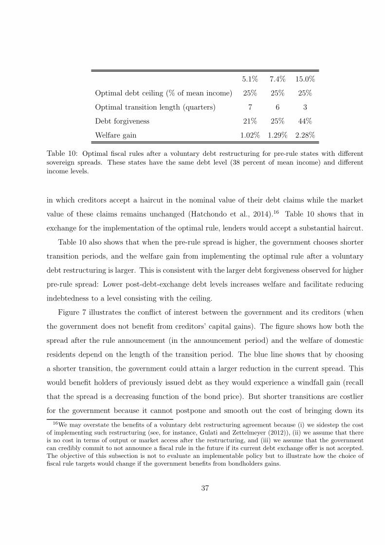
We find that when the government benefits from the appreciation of the value of debt issued

prior to the rule announcement, it chooses a lower debt ceiling with a shorter transition period.

Table 10 shows that for three pre-rule states we consider, the government chooses a 25 percent

ceiling that is enforced less than two years after its announcement. This contrasts with the 30

percent debt limit to be enforced more than four-years after of the rule announcement that is

optimal when the government does not benefit from bondholders gains (Table 8).

The exercise presented in this subsection can be thought of as a voluntary debt restructuring

36

5.1% 7.4% 15.0%

Optimal debt ceiling (% of mean income) 25% 25% 25%

Optimal transition length (quarters) 7 6 3

Debt forgiveness 21% 25% 44%

Welfare gain 1.02% 1.29% 2.28%

Table 10: Optimal fiscal rules after a voluntary debt restructuring for pre-rule states with differentsovereign spreads. These states have the same debt level (38 percent of mean income) and differentincome levels.

in which creditors accept a haircut in the nominal value of their debt claims while the market

value of these claims remains unchanged (Hatchondo et al., 2014).16 Table 10 shows that in

exchange for the implementation of the optimal rule, lenders would accept a substantial haircut.

Table 10 also shows that when the pre-rule spread is higher, the government chooses shorter

transition periods, and the welfare gain from implementing the optimal rule after a voluntary

debt restructuring is larger. This is consistent with the larger debt forgiveness observed for higher

pre-rule spread: Lower post-debt-exchange debt levels increases welfare and facilitate reducing

indebtedness to a level consisting with the ceiling.

Figure 7 illustrates the conflict of interest between the government and its creditors (when

the government does not benefit from creditors’ capital gains). The figure shows how both the

spread after the rule announcement (in the announcement period) and the welfare of domestic

residents depend on the length of the transition period. The blue line shows that by choosing

a shorter transition, the government could attain a larger reduction in the current spread. This

would benefit holders of previously issued debt as they would experience a windfall gain (recall

that the spread is a decreasing function of the bond price). But shorter transitions are costlier

for the government because it cannot postpone and smooth out the cost of bringing down its

16We may overstate the benefits of a voluntary debt restructuring agreement because (i) we sidestep the costof implementing such restructuring (see, for instance, Gulati and Zettelmeyer (2012)), (ii) we assume that thereis no cost in terms of output or market access after the restructuring, and (iii) we assume that the governmentcan credibly commit to not announce a fiscal rule in the future if its current debt exchange offer is not accepted.The objective of this subsection is not to evaluate an implementable policy but to illustrate how the choice offiscal rule targets would change if the government benefits from bondholders gains.

37

debt level. Thus, compared with the government, creditors prefer a shorter transition period and

a lower debt ceiling.

0 1 2 3 4 5 6 7 80

1

2

3

4

5

6

7

8

Spr

ead

Spread before the announcementSpread after the announcementWelfare gain

1 2 3 4 5 6 7 8−0.15

−0.1

−0.05

0

0.05

0.1

0.15

0.2

0.25

Years before the ceiling starts binding

Wel

fare

gai

n (%

con

s.)

Figure 7: Spread after the implementation of a rule with a ceiling of 30 percent of mean income, whenthe debt is 38 percent of mean income and the pre-rule spread is 7.4 percent.

5.13 Shortsighted governments

In this subsection we discuss the extent to which our finding would change in it is assumed that

governments are shortsighted. Shortsighted governments (for instance, because of political polar-

ization and political turnover) are typically mentioned as a justification for fiscal rules. Previous

subsections show that fiscal rules can be beneficial even without shortsighted government. This

subsection shows that assuming shortsighted governments reinforce our results: it is optimal to

introduce fiscal rules that lower the sovereign default premium to negligible levels.

To gauge the role of government’s myopia we assume that the fiscal rule is chosen by a planer

that discount the future with a β higher than the one governments use each period when the

choose their fiscal policy. For instance, one may think that the political coalition necessary to

establish a fiscal rule in the constitution requires a majority that mitigates the effects of political

polarization when discounting future outcomes (for a discussion of the effects of polarization

38

on fiscal dynamics see Azzimonti, 2011). In particular, we assume that the planner discounts

the future with β = 0.99 (while as in the benchmark governments optimize each period with

β = 0.961). We repeat the exercise proposed in Subsection 5.9. That is, (i) we consider a

pre-rule state characterized by a debt level of 38 percent of trend annual income and an income

level that gives us a spread of 7.4 percent, (ii) we assume that rules impose a transition period

with a per-period debt reduction of 0.5 percent of trend income, and a fixed debt limit after

the transition, and (iii) we let the government choose the length of the transition period and,

therefore, its long-run debt limit.

Table 11 presents the optimal fiscal rule chosen by a planer who is more patient than short-

sighted governments. Of course, when the rule chosen giving more weight to future periods

imposes stronger fiscal adjustments. In particular the rule chosen by the planer completely elim-

inates default risk and thus promotes a countercyclical fiscal policy). Table 11 also shows that

the welfare gain from introducing a fiscal rules is much higher when we assume the rule corrects

government’s myopia.

Governments Planer

Announcement-period spread (pre announcement) 7.4% 7.4%

Optimal transition length (quarters) 36 56

Optimal debt ceiling after the transition (% of trend annual income) 20% 10%

Announcement-period spread (post announcement) 0.5% 0.2%

Long-run average spread 0.5% 0.0%

Welfare gain 0.25% 3.50%

Table 11: Optimal fiscal rule with shortsighted governments.

6 Conclusions

We use a standard sovereign default framework to show that there may be substantial gains from

committing to fiscal rules. We also argue that fiscal rules targeting the level of the sovereign

39

default premium are preferable over rules targeting sovereign debt levels (as most fiscal rules do

in reality). While optimal debt limits vary greatly across parameterizations of the model that

determine the level of debt tolerance, optimal sovereign-premium limits are very similar across

parameterizations. Since the level of debt tolerance in the data is difficult to identify, and seem

to vary greatly both across countries and over time, spread-targeting fiscal rules are likely to

perform better than debt-targeting fiscal rules.

The paper present several other results that speak to important fiscal policy debates. We

show that rules allow the government to implement a less procyclical fiscal policy but should not

necessarily promote a countercyclical fiscal policy. We illustrate the importance of establishing

intermediate fiscal adjustment targets when rules are introduced. Furthermore, we show how

introducing rules can result in reductions of the levels of debt and sovereign default premium

without any fiscal adjustment (and even with fiscal expansions). In addition, we demonstrate

that benefits from imposing a rule arise even if the government is not shortsighted.

We chose to make our analysis more transparent by respecting the simplifying assumptions

commonly used in quantitative studies of sovereign defaults. Future work could enrich our

analysis by relaxing these assumptions.

One interesting extension of our work could be to study the impact of less-than-perfectly-

credible fiscal rules. For instance, we abstract from political shocks that could threaten the

enforcement of a rule (Alfaro and Kanczuk (2005), Amador (2003), Cole et al. (1995), Cuadra

and Sapriza (2008), D’Erasmo (2008), and Hatchondo et al. (2009) study sovereign default models

with political shocks).

As in Chatterjee and Eyigungor (2012) and Hatchondo and Martinez (2009), we assumed

that the government cannot choose the duration of its debt. Relaxing this assumption could

enhance our understanding of the effects of fiscal rules but it would increase the computation

cost significantly.17

17In order to allow the government to choose a different duration of its debt, one would have to introduce bondsof different duration and keep track of how many of each of these bonds the government has issued (see Arellanoand Ramanarayanan (2010)). The computation cost of including additional state variables may be significant(Hatchondo et al. (2010a) show that the computation cost of obtaining accurate solutions in default models maybe significant, and Chatterjee and Eyigungor (2012) explain how the cost increases when long-duration bonds areassumed).

40

Extending our framework to include production could also improve the understanding of

the effects of fiscal rules. We found large effects of fiscal rules on the level and volatility of

interest rates. Several studies find significant effects of the interest rate on productivity (through

investment and the allocation of factors of production), and of interest rate fluctuations on the

amplification of shocks (see, for example, Mendoza and Yue (2012), Neumeyer and Perri (2005),

and Uribe and Yue (2006)). Since there is no production in our setup, we do not allow for these

channels. Furthermore, our analysis of the cyclicality of fiscal policy is limited because fiscal

policy does not play a role in stabilizing aggregate income.

Studying a setup in which the sovereign simultaneously holds assets and liabilities may also

be an interesting avenue for future research. Fiscal rules often aim at controlling the sovereign’s

accumulation of both assets and liabilities. For simplicity, as is standard in default models,

we assume that the government cannot simultaneously have assets and liabilities (Alfaro and

Kanczuk (2009) and Bianchi et al. (2012) study a sovereign default model where the government

can simultaneously hold assets and liabilities).

41

References

Adler, G. and Sosa, S. (2013). ‘Debt Sustainability in Latin America: How Dependent on

External Conditions?’ IMF Working Paper.

Aguiar, M. and Gopinath, G. (2006). ‘Defaultable debt, interest rates and the current account’.

Journal of International Economics , volume 69, 64–83.

Aguiar, M. and Gopinath, G. (2007). ‘Emerging markets business cycles: the cycle is the trend’.

Journal of Political Economy , volume 115, no. 1, 69–102.

Alfaro, L. and Kanczuk, F. (2005). ‘Sovereign debt as a contingent claim: a quantitative ap-

proach’. Journal of International Economics , volume 65, 297 314.

Alfaro, L. and Kanczuk, F. (2009). ‘Optimal reserve management and sovereign debt’. Journal

of International Economics , volume 77(1), 23–36.

Alvarez, F. A., Marques, L. B., and Toledo, M. (2011). ‘Business Cycles in Emerging Markets:

The Role of Durable Goods and Financial Frictions’. Manuscript, Universidad Carlos III.

Amador, M. (2003). ‘A Political Economy Model of Sovereign Debt Repayment’. Manuscript,

Stanford University.

Arellano, C. (2008). ‘Default Risk and Income Fluctuations in Emerging Economies’. American

Economic Review , volume 98(3), 690–712.

Arellano, C. and Ramanarayanan, A. (2010). ‘Default and the Maturity Structure in Sovereign

Bonds’. Mimeo, University of Minnesota.

Athreya, K., Tam, X. S., and Young, E. R. (2007). ‘Does Rising Income Risk Lead to Better

Risk Sharing?’ Manuscript, University of Virginia.

Azzimonti, M. (2011). ‘Barriers to Investment in Polarized Societies’. American Economic

Review , volume 101, 2182–2204. 5.

42

Azzimonti, M., Battaglini, M., and Coate, S. (2010). ‘On the Case for a Balanced Budget

Amendment to the U.S. Constitution’. Mimeo, Princeton University.

Backus, D., Foresi, S., and Telmer, C. (1998). ‘Discrete-time models of bond pricing’. NBER

Working Paper 6736.

Beetsma, R. and Debrun, X. (2007). ‘The new stability and growth pact: A first assessment’.

European Economic Review , volume 51, 453–477.

Beetsma, R. and Uhlig, H. (1999). ‘An Analysis of the Stability and Growth Pact’. The Economic

Journal , volume 109(458), 546–571.

Benjamin, D. and Wright, M. L. J. (2008). ‘Recovery Before Redemption? A Theory of Delays

in Sovereign Debt Renegotiations’. Manuscript.

Bi, H. (2011). ‘Sovereign default risk premia, fiscal limits and fiscal policy’. European Economic

Review . Forthcoming.

Bi, H. and Leeper, E. (2012). ‘Analyzing fiscal sustainability’. Working Paper.

Bianchi, J., Hatchondo, J. C., and Martinez, L. (2012). ‘International Reserves and Rollover

Risk’. NBER Working Paper 18628.

Blanchard, O. (2011). ‘Rewriting the Macroeconomists’ Playbook in the Wake of the Crisis’.

IMFdirect.

Blanchard, O., Dell’Ariccia, G., and Mauro, P. (2010). ‘Rethinking Macroeconomic Policy’. IMF

Staff Position Note 10/03.

Borri, N. and Verdelhan, A. (2009). ‘Sovereign Risk Premia’. Manuscript, MIT.

Boz, E. (2011). ‘Sovereign Default, Private Sector Creditors, and the IFIs’. Journal of Interna-

tional Economics , volume 83, 70–82.

Boz, E., Daude, C., and Durdu, B. (2011). ‘Emerging Market Business Cycles Revisited: Learning

about the Trend’. Journal of Monetary Economics , volume 58, 616–631.

43

Broner, F. A., Lorenzoni, G., and Schmukler, S. L. (2007). ‘Why do emerging economies borrow

short term?’ National Bureau of Economic Research Working Paper 13076.

Budina, N., Kinda, T., Schaechter, A., and Weber, A. (2012). ‘Fiscal Rules at a Glance: Country

Details from a New Dataset’. IMF Working Paper 12/273.

Calvo, G. (1988). ‘Servicing the Public Debt: The Role of Expectations’. The American Eco-

nomic Review , volume 78 (4), 647–661.

Chatterjee, S., Corbae, D., Nakajima, M., and Rıos-Rull, J.-V. (2007). ‘A Quantitative Theory

of Unsecured Consumer Credit with Risk of Default’. Econometrica, volume 75, 1525–1589.

Chatterjee, S. and Eyigungor, B. (2012). ‘Maturity, Indebtedness and Default Risk’. American

Economic Review , volume 102(6), 2674–2699.

Chatterjee, S. and Eyigungor, B. (2013). ‘Debt Dilution and Seniority in a Model of Defaultable

Sovereign Debt’. Federal Reserve Bank of Philadelphia Working Paper 13-30.

Claessens, S., Mody, A., and Vallee, S. (2012). ‘Paths to Eurobonds’. IMF Working Paper

12/172.

Cole, H., Dow, J., and English, W. (1995). ‘Default, settlement, and signaling: lending resump-

tion in a reputational model of sovereign debt’. International Economic Review , volume 36,

no. 2, 365–385.

Corbacho, A. and Schwartz, G. (2007). ‘Fiscal Responsibility Laws’. in Promoting Fiscal Disci-

pline, volume Ter-Minassian, T. and M. S. Kumar (eds.).

Cruces, J. J., Buscaglia, M., and Alonso, J. (2002). ‘The Term Structure of Country Risk and

Valuation in Emerging Markets’. Manuscript, Universidad Nacional de La Plata.

Cuadra, G., Sanchez, J. M., and Sapriza, H. (2010). ‘Fiscal policy and default risk in emerging

markets’. Review of Economic Dynamics , volume 13(2), 452–469.

44

Cuadra, G. and Sapriza, H. (2008). ‘Sovereign default, interest rates and political uncertainty in

emerging markets’. Journal of International Economics , volume 76, 78–88.

Debrun, X. and Kumar, M. S. (2007). ‘Fiscal Rules, Fiscal Councils and All That: Commitment

Devices, Signaling Tools or Smokescreens?’ in Fiscal Policy: Current Issues and Challenges ,

volume Banca dItalia (eds.).

Debrun, X., Moulin, L., Turrini, A., Ayuso-i Casals, J., and Kumar, M. S. (2008). ‘Tied to the

mast? National fiscal rules in the European Union’. Economic Polic, volume 23(54), 297–362.

D’Erasmo, P. (2008). ‘Government Reputation and Debt Repayment in Emerging Economies’.

Manuscript, University of Texas at Austin.

Deroose, S., Moulin, L., and Wierts, P. (2006). ‘National expenditure rules and expenditure

outcomes: Evidence for EU member states’. Wirtschaftspolitische Bltter , volume 53.

Dias, D. A. and Richmond, C. (2007). ‘Duration of Capital Market Exclusion: An Empirical

Investigation’. Working Paper, UCLA.

Eaton, J. and Gersovitz, M. (1981). ‘Debt with potential repudiation: theoretical and empirical

analysis’. Review of Economic Studies , volume 48, 289–309.

EC (2006). ‘Public nances in EMU’. European Commission. No. 3.

Eichengreen, B. and Bayoumi, T. (1994). ‘The political economy of fiscal restrictions: Implica-

tions for Europe from the United States’. European Economic Review , volume 38, 783–791.

Garcia, C. J., Restrepo, J. E., and Tanner, E. (2011). ‘Fiscal rules in a volatile world: A

welfare-based approach’. Journal of Policy Modeling , volume 33, 649–676.

Gavin, M. and Perotti, R. (1997). ‘Fiscal Policy in Latin America’. NBER Macroeconomics

Annual , pages 11–71.

Ghosh, A. R., Kim, J. I., Mendoza, E. G., Ostry, J. D., and Qureshi, M. S. (2011). ‘Fiscal Fatigue,

Fiscal Space and Debt Sustainability in Advanced Economies’. NBER Working Paper 16782.

45

Gonzalez-Rozada, M. and Levy Yeyati, E. (2008). ‘Global factors and emerging market spreads’.

Economic Journal , volume 118, 1917–1936.

Gulati, M. and Zettelmeyer, J. (2012). ‘Making a Voluntary Greek Debt Exchange Work’.

Mimemo, Duke University.

Hatchondo, J. C. and Martinez, L. (2009). ‘Long-duration bonds and sovereign defaults’. Journal

of International Economics , volume 79, 117–125.

Hatchondo, J. C. and Martinez, L. (2012). ‘On the Benefits of GDP-Indexed Government Debt:

Lessons from a Model of Sovereign Defaults’. Economic Quarterly , volume 98, 139–157. No.

2.

Hatchondo, J. C., Martinez, L., and Sapriza, H. (2007). ‘Quantitative Models of Sovereign

Default and the Threat of Financial Exclusion’. Economic Quarterly , volume 93, 251–286.

No. 3.

Hatchondo, J. C., Martinez, L., and Sapriza, H. (2009). ‘Heterogeneous borrowers in quantitative

models of sovereign default.’ International Economic Review , volume 50, 1129–1151.

Hatchondo, J. C., Martinez, L., and Sapriza, H. (2010a). ‘Quantitative properties of sovereign

default models: solution methods matter’. Review of Economic Dynamics , volume 13, no. 4,

919–933.

Hatchondo, J. C., Martinez, L., and Sosa Padilla, C. (2010b). ‘Debt dilution and sovereign

default risk’. Federal Reserve Bank of Richmond Working Paper 10-08R.

Hatchondo, J. C., Martinez, L., and Sosa Padilla, C. (2014). ‘Voluntary Sovereign Debt Ex-

changes’. volume 61, 32–50.

Heinemann, F., Kalb, A., and Osterloh, S. (2011). ‘Sovereign risk premia: the link between fiscal

rules and stability culture’. Mimeo, ZEW Mannheim.

Iara, A. and Wolff, G. (2011). ‘Rules and risk in the euro area’. Bruegel Working Paper 2011/10,

Brussels.

46

Ilzetzki, E., Mendoza, E. G., and Vegh, C. A. (2012). ‘How big (small?) are scal multipliers?’

Journal of Monetary Economics .

IMF (2009). ‘Fiscal Rules: Anchoring Expectations for Sustainable Public Finances’. Fiscal

Affairs Department, International Monetary Fund.

IMF (2012). ‘Fiscal Monitor: Balancing Fiscal Policy Risks’. April.

IMF (2013a). ‘Fiscal Monitor: Fiscal Adjustment in an Uncertain World’. April.

IMF (2013b). ‘Staff Guidance Note for Public Debt Sustainability Analysis in Market-Access

Countries’. International Monetary Fund.

IMF (2013c). ‘Staff Guidance Note on the Application of the Joint Bank-Fund Debt Sustainability

Framework for Low-Income Countries’. International Monetary Fund.

Kaminsky, G., Reinhart, C., and Vegh, C. (2004). ‘When It Rains, It Pours: Procyclical Capital

Flows and Macroeconomic Policies’. NBER Macroeconomics Annual , pages 11–53.

Kopits, G. (2004). ‘Overview of Fiscal Policy Rules in Emerging Markets’. in Rules-Based Fiscal

Policy in Emerging Markets. Background, Analysis, and Prospects , volume Kopits, G. (ed.).

Krusell, P. and Smith, A. (2003). ‘Consumption-savings decisions with quasi-geometric discount-

ing’. Econometrica, volume 71, no. 1, 365–375.

Li, W. and Sarte, P.-D. (2006). ‘U.S. consumer bankruptcy choice: The importance of general

equilibrium effects’. Journal of Monetary Economics , volume 53, 613–631.

Livshits, I., MacGee, J., and Tertilt, M. (2008). ‘Consumer Bankruptcy: A Fresh Start,’. Amer-

ican Economic Review , volume 97, 402–418.

Lizarazo, S. (2005). ‘Sovereign risk and risk averse international investors’. Working Paper,

ITAM.

Lizarazo, S. (2006). ‘Contagion of financial crises in sovereign debt markets’. Working Paper,

ITAM.

47

Longstaff, F. A., Pan, J., Pedersen, L. H., and Singleton, K. J. (2011). ‘How Sovereign is

Sovereign Credit Risk?’ American Economic Journal: Macroeconomics , volume 3(2), 75–103.

Lowry, R. and Alt, J. (2001). ‘A visible hand? Bond markets, political parties, balanced budget

laws, and state government debt’. Economics & Politics , volume 13(1), 49–72.

Medina, J. P. and Soto, C. (2007). ‘Copper price, fiscal policy, and busines cycle in Chile’.

Central Bank of Chile Working Paper 458.

Mendoza, E. and Yue, V. (2012). ‘A General Equilibrium Model of Sovereign Default and

Business Cycles’. The Quarterly Journal of Economics . Forthcoming.

Neumeyer, P. and Perri, F. (2005). ‘Business cycles in emerging economies: the role of interest

rates’. Journal of Monetary Economics , volume 52, 345–380.

Pappa, E. and Vassilatos, V. (2007). ‘The unbearable tightness of being in a monetary union:

Fiscal restrictions and regional stability’. European Economic Review , volume 51, 1492–1513.

Poplawski Ribeiro, M., Beetsma, R., and Schabert, A. (2008). ‘A Comparison of Debt and

Primary-deficit Constraints’. CEPR Discussion Paper No. 6897.

Poterba, J. (1996). ‘Budget Institutions and Fiscal Policy in the U.S. States’. American Economic

Review , volume 86(2), 395–400.

Poterba, J. M. and Rueben, K. (1999). ‘State fiscal institutions and the U.S. municipal bond

market’. In Fiscal Institutions and Fiscal Performance, James Poterba and Jrgen von Hagen

editors, University of Chicago Press.

Reinhart, C., Rogoff, K. S., and Savastano, M. A. (2003). ‘Debt Intolerance’. Brookings Papers

on Economic Activity .

Sanchez, J. M. (2010). ‘The IT Revolution and the Unsecured Credit Market’. Federal Reserve

Bank of St. Louis Working Paper.

48

Schaechter, A., Kinda, T., Budina, N., and Weber, A. (2012). ‘Fiscal Rules in Response to the

CrisisToward the Next-Generation Rules. A New Dataset’. IMF Working Paper 12/187.

Talvi, E. and Vegh, C. (2009). ‘Tax Base Variability and Procyclicality of Fiscal Policy’. Journal

of Development Economics , volume 78(1), 156–90.

Tanner, E. and Samake, I. (2006). ‘Probabilistic Sustainability of Public Debt: A Vector Au-

toregression Approach for Brazil, Mexico, and Turkey’. IMF Working Paper 06/295.

Uribe, M. and Yue, V. (2006). ‘Country spreads and emerging countries: Who drives whom?’

Journal of International Economics , volume 69, 6–36.

Vasicek, O. (1977). ‘An equilibrium characterization of the term structure’. Journal of Financial

Economics , volume 5, 177–188.

Vegh, C. A. and Vuletin, G. (2011). ‘How is tax policy conducted over the business cycle?’

Mimeo, University of Maryland.

Yue, V. (2010). ‘Sovereign default and debt renegotiation’. Journal of International Economics ,

volume 80, no. 2, 176–187.

49