Kinematic structure of massive star-forming regions - I ...beuther/tackenberg2014.pdftory, has shed...

Astronomy & Astrophysics manuscript no. n2hp_mapping c©ESO 2014January 9, 2014

Kinematic structure of massive star-forming regions - I. Accretion

along filaments

J. Tackenberg1, H. Beuther1, Th. Henning1, H. Linz1, T. Sakai2, S. E. Ragan1, O. Krause1, M. Nielbock1, M.

Hennemann1, 3, J. Pitann1, A. Schmiedeke1, 4

1 Max-Planck-Institut für Astronomie (MPIA), Königstuhl 17, 69117 Heidelberg, Germanye-mail: [email protected]

2 Graduate School of Informatics and Engineering, The University of Electro-Communications, Chofu, Tokyo 182-8585, Japan3 AIM Paris-Saclay, CEA/DSM/IRFU – CNRS/INSU – Université Paris Diderot, CEA Saclay, 91191 Gif-sur-Yvette cedex, France4 Universität zu Köln, Zülpicher Str. 77, 50937, Köln, Germany

Received September 15, 1996; accepted March 16, 1997

ABSTRACT

Context. The mid- and far-infrared view on high-mass star formation, in particular with the results from the Herschel space observa-tory, has shed light on many aspects of massive star formation. However, these continuum studies lack kinematic information.Aims. We study the kinematics of the molecular gas in high-mass star-forming regions.Methods. We complement the PACS and SPIRE far-infrared data of 16 high-mass star-forming regions from the Herschel Key projectEPoS with N2H+ molecular line data from the MOPRA and Nobeyama 45m telescope. Using the full N2H+ hyperfine structure, weproduce column density, velocity, and linewidth maps. These are correlated with PACS 70 µm images and PACS point sources. Inaddition, we search for velocity gradients.Results. For several regions, the data suggest that the linewidth on the scale of clumps is dominated by outflows or unresolvedvelocity gradients. IRDC 18454 and G11.11 show two velocity components along several line-of-sights. We find that all regionswith a diameter larger than 1 pc show either velocity gradients or fragment into independent structures with distinct velocities. Thevelocity profiles of 3 regions with a smooth gradient are consistent with gas flows along the filament, suggesting accretion flows ontothe densest regions.Conclusions. We show that the kinematics of several regions show significant and complex velocity structure. For three filaments,we suggest that gas flows toward the more massive clumps are present.

Key words. Stars:formation, kinematics and dynamics

1. Introduction

Despite their rarity, high-mass stars are important for all fieldsof astronomy. Within the Milky Way they shape and regulate theformation of clusters, influence the chemistry of the interstellarmedium, and might have even affected the formation of the solarsystem (Gritschneder et al. 2012). On the larger scales, emissionfrom high-mass stars dominates the emission detected from ex-ternal galaxies. In addition, massive stars are the origin of heavyelements on all scales. Nevertheless, high-mass star formationis far from understood (Beuther et al. 2007; Zinnecker & Yorke2007).

Sensitive IR and (sub-) mm Galactic plane surveys togetherwith results from the Herschel1 space observatory (Pilbrattet al. 2010) have shed new light on the cradles of massivestars/clusters and their early formation. Perault et al. (1996) andEgan et al. (1998) discovered extinction patches in the brightmid-IR background using the ISO (Kessler et al. 1996) and MSX(Egan et al. 2003) satellites, similar to the dark patches reportedby Barnard (1919) which are today known to be connected tolow-mass star formation. Soon after, Carey et al. (1998) es-tablished the so-called infrared dark clouds (IRDCs) as precur-

1 Herschel is an ESA space observatory with science instruments pro-vided by European-led Principal Investigator consortia and with impor-tant participation from NASA.

sors of high-mass star formation. Today, the Spitzer observatoryGalactic plane surveys GLIMPSE at 3.6 µm, 4.5 µm, 5.8 µm, and8 µm (Benjamin et al. 2003), and MIPSGAL at 24 µm (Careyet al. 2009) allow the systematic search for IRDCs with unprece-dented sensitivity (e.g. Peretto & Fuller 2009).

While Spitzer improved our mid-IR view of the Galaxy, theHerschel satellite allows observations of the far-IR. With thePACS (Poglitsch et al. 2010) and SPIRE (Griffin et al. 2010)photometer, high sensitivity and spatial resolution observationsbetween 70 µm and 500 µm are possible. From correlating dataat mid-IR through sub-millimeter and millimeter wavelengths,the picture emerged that most star-forming regions are filamen-tary (André et al. 2010; Men’shchikov et al. 2010; Molinari et al.2010; Schneider et al. 2010; Hill et al. 2011; Hennemann et al.2012; Peretto et al. 2012).

In numerical studies, the formation of dense cores andclumps is explained by two scenarios. On the one hand, molec-ular clouds fragment in a self-similar cascade down to the typ-ical size of dense, quasi-static cores supported by turbulence.These will then form single or multiple gravitationally boundobjects (McKee & Tan 2003; Zinnecker & Yorke 2007). On theother hand, in the dynamical theory molecular clouds are formedfrom large-scale flows of atomic gas as transient objects (MacLow & Klessen 2004; Klessen et al. 2005; Heitsch & Hartmann2008; Clark et al. 2012). Within these transient structures, su-

Article number, page 1 of 25

personic turbulence compresses some fraction of the gas to fila-ments, clumps, and dense cores. If gravity dominates, the corescollapse. In contrast to the quasi-static cores, these cores con-stantly grow in mass. If, by chance, some cores accrete massfaster than others due to their higher initial gravitational poten-tial, this is called competitive accretion (Bonnell et al. 2004).Also dynamical, but of reversed reasoning, in the fragmentation-induced starvation scenario by Peters et al. (2010), individualmassive dense cores build from the large-scale flows, and an ac-companying cluster of smaller cores drag away material from themain core and diminish its mass accretion.

The Earliest Phases of Star formation (EPoS, PI O. Krause)is a Guaranteed Time Herschel Key Program for investigating14 low-mass and 45 high-mass star-forming regions. The low-mass observations have been summarized in Launhardt et al.(2013), and the high-mass part has been described in Ragan et al.(2012a). The high-mass part of the project provides an excellenttarget list for studying the kinematics in star-forming regions.This is the ultimate goal of this paper, using N2H+ molecularline data.

2. Observations and analysis

2.1. EPoS - A Herschel Key Project

All 45 high-mass EPoS sources were observed with the Her-schel satellite (Pilbratt et al. 2010) at 70 µm, 100 µm, 160 µm,250 µm, 350 µm, and 500 µm with a spatial resolution of 5.6′′,6.8′′, 11.3′′, 18.1′′, 25.2′′, and 36.6′′, respectively (Poglitschet al. 2010; Griffin et al. 2010). The observations were performedin two orthogonal directions and the data reduction has beenperformed using HIPE (Ott 2010) and scanamorphos (Roussel2012). A more detailed description of the data reduction is givenin Ragan et al. (2012a).

Out of the 45 Herschel EPoS high-mass sources we selecteda sub-sample of 17 regions given in Table 1 that cover each im-portant evolutionary stage: promising high-mass starless corecandidates, IRDCs with weak mid- and far-infrared sources, in-dicative of early ongoing star formation activity, and knownhigh-mass protostellar objects (HMPOs).

The protostellar core population was already characterized inRagan et al. (2012a) using Herschel photometry, supplementedby Spitzer, IRAS, and MSX data. By modeling the spectral en-ergy distributions (SEDs), the authors fit the temperature, lumi-nosity, and mass of each protostellar core in the sample.

2.2. Nobeyama 45m observations

Between April 7th and 12th 2010 the BEam Array Receiver Sys-tem (BEARS, Sunada et al. 2000) on the Nobeyama Radio Ob-servatory (NRO2) 45 m telescope was used to map six of the re-gions in N2H+; the details are given in Table 1. At a frequencyof the N2H+ (1-0) transition of 93.173 GHz, the spatial resolu-tion of the NRO 45 m telescope is 18′′(HPBW) and the observ-ing mode with a band-width of 32 MHz has a frequency resolu-tion of 62.5 kHz, or 0.2 km/s. All observations were performedusing on-the-fly (OTF) mapping in varying weather conditions,with an average system temperature of 280 K and high precip-itable water vapors between 3 mm and 9 mm. The pointing wasdone using the single pixel receiver S40 tuned to SiO. As point-ing sources we used the SiO masers of the late-type stars V468

2 Nobeyama Radio Observatory is a branch of the National Astronom-ical Observatory of Japan, National Institutes of Natural Sciences.

Cyg, IRC+00363, and R Aql. Although the wind conditionscontributed to the pointing uncertainties, the pointing is betterthan a third of the beam.

For the data reduction we used NOSTAR (Sawada et al.2008), a software package provided by the NRO for OTF data.The data is sampled to a spatial grid of 7.5′′and smoothed to aspectral resolution of 0.5 km/s. To account for the different ef-ficiencies of the 25 receivers in the BEARS array we correctedeach pixel to the efficiency of the S100 receiver, using individualcorrection factors and a beam efficiency of η = 0.46 to calculatemain-beam temperatures. The noisy edges due to less coveragehave been removed within NOSTAR by suppressing pixels in thefinal maps with a rms noise above 0.15 K. The resulting antennatemperature maps have an average rms noise between 0.12 K and0.13 K per beam.

2.3. MOPRA observations

11 sources, listed in Table 1, were mapped with the 22 m MO-PRA radio telescope, operated by the Australia Telescope Na-tional Facility (ATNF) in OTF mode. The observations werecarried out in 2010, June 1st to 5th and 25th to 27th, as wellas July 7th through 9th. High precipitable water vapors duringthe observations result in system temperatures mostly between200 K and 300 K. Observations with system temperatures above500 K were ignored during the data reduction.

We employed 13 of the MOPRA spectrometer (MOPS)zoom bands, each of 138 MHz width and 4096 channels, result-ing in a velocity resolution of 0.11 km/s at 90 GHz. The spectralsetup covered transitions of CH3CCH, H13CN, H13CO+, SiO,C2H, HNCO, HCN, HCO+, HNC, HCCCN, CH3CN, 13CS, andN2H+ in the 90 GHz regime (for details on the transitions andtheir excitation conditions see Vasyunina et al. 2011). At thiswavelength, the MOPRA beam FWHM is 35.5′′and the beam ef-ficiency is assumed to be constant over the frequency range withη = 0.49 (Ladd et al. 2005). The data reduction was done usingLIVEDATA and GRIDZILLA, an on-the-fly mapping analysispackage provided by the ATNF. In order to improve the signal-to-noise ratio we spatially smoothed the data to a beam FWHMof 46′′within (and as suggested by) gridzilla. The final mapswere smoothed to a spectral resolution of 0.21 km/s - 0.23 km/s(depending on the transition frequency). Spectra with an rmsnoise above 0.12 K have been removed, affecting pixels at theedges. The resulting average rms noise of the individual maps isthen below 0.09 K/beam.

However, the observed regions of interest are dense but stillcold. Therefore, with the achieved sensitivity at the given spatialresolution we do not detect the more complex or low-abundancemolecules. For example, although SiO (2-1) has been detectedtoward several positions that we have mapped (Sridharan et al.2002; Sakai et al. 2010), the strongest SiO emitter found by Linzet al. (in prep., G28.34-2) is at our noise level and thereforenot detected. Commonly detected and reasonably mapped areHCN (1-0), HNC (1-0), HCO+ (1-0), H13CO+ (1-0), and N2H+

(1-0). As we discuss in Sect. 2.5, we concentrate on N2H+, awell known cold dense gas tracer.

2.4. Dust continuum

In order to trace the total cold gas we use the cold dust emis-sion as a tracer of the molecular gas. As most of the selectedsources lie within the Galactic plane, the APEX 870 µm surveyATLASGAL (Schuller et al. 2009; Contreras et al. 2013) cov-


J. Tackenberg et al., 2013: Flows along massive star-forming regions

Table 1. Observed IRDCs.

Source RA(J2000) DEC(J2000) Gal.longitude

Gal. lati-tude

Distance beamsize

minimumN2H+

detection

minimumN2H+ detec-tion 0.4 km/s

name [ hh mm ss.s ] [ dd:mm:ss ] [ ] [ ] [ kpc ] [ pc ]× 1012 cm−2 × 1012 cm−2

Observed with Nobeyama 45mIRDC 18223 18 25 10.7 -12 45 12 18.613 -0.081 3.5 0.3 0.8IRDC 18310 18 33 44.7 -08 22 36 23.467 0.085 4.9 0.4 3.9IRDC 18385 18 41 17.1 -05 09 15 27.189 -0.098 3.1 0.3 1.2IRDC 18454 18 47 58.1 -01 54 41 30.835 -0.100 5.3 0.5 4.1

ISOSS J20153 20 15 21.4 +34 53 52 72.953 -0.027 1.2 0.1 8.1IRDC 13.90 18 17 26.1 -17 05 26 13.906 -0.473 2.6 0.2 1.4

Observed with MopraIRDC 18102 18 13 12.2 -17 59 34 12.632 -0.016 2.6 0.6 5.7 3.3IRDC 18151 18 17 55.3 -12 07 29 18.335 1.778 2.7 0.6 3.9 2.8IRDC 18182 18 21 12.2 -14 32 46 16.577 -0.069 3.4 0.7 3.2 2.2IRDC 18306 18 33 29.9 -08 32 07 23.298 0.066 3.6 0.8 1.5 1.6IRDC 18308 18 33 33.1 -08 37 46 23.220 0.011 4.4 1.0 2.9 2.1IRDC 18337 18 36 29.6 -07 40 33 24.402 -0.197 3.7 0.8 1.8 1.1IRDC 19.30 18 25 58.1 -12 05 09 19.293 0.060 2.4 0.5 7.6 1.3IRDC 11.11 18 10 20.0 -19 25 05 11.056 -0.107 3.4 0.7 2.4 1.6IRDC 15.05 18 17 40.4 -15 49 12 15.052 0.080 3.0 0.7 3.4 1.4IRDC 28.34 18 42 48.1 -04 01 51 28.361 0.080 4.5 1.0 4.5 3.2IRDC 48.66 19 21 40.7 +13 50 32 48.666 -0.263 2.6 0.6 2.3 0.8

Position columns (2-5) give the center coordinate of the maps. The actual areas that have been mapped are displayed in Fig. 1 through Fig. 4. Thedistances are adopted from (Ragan et al. 2012a) with references therein. The detected N2H+ minimum the minimum plotted in Fig. 1 through

Fig. 4. For sources observed with MOPRA we also give the improved minimum detection when smoothing the spectra to a velocity resolution of0.4 km/s. Also observed with the NRO 45m telescope but not detected have been IRDC20081, ISOSSJ19357, ISOSSJ19557, and ISOSSJ20093.

ers all but two sources. Its beam size is 19.2′′and its averagerms noise is 50 mJy/beam. IRDC 18151 with a Galactic latitudeof ∼ 1.7is not covered by ATLASGAL. Instead we use IRAM30 m MAMBO data (Beuther et al. 2002b). At a wavelength of1.2 mm, the beam width is 10.5′′, and the rms noise in the dustmap is 17 mJy/beam. In addition, ISOSS J20153 is outside thecoverage of ATLASGAL. Here we used 850 µm data from theSCUBA camera at the JCMT3 (Hennemann et al. 2008). Thebeam width is 14′′and the rms noise 14 mJy/beam. A summaryof the properties of the sub-mm data is given in Table 2.

2.5. N2H+ hyperfine fitting

Our molecular line study focuses on the N2H+ J=1-0 line asdense molecular gas tracer. Using the Einstein A and collisoncoefficient for a temperature of 20 K (Schöier et al. 2005), itscritical density is 1.6× 105 cm−3, and its hyperfine structure al-lows one to reliably measure its optical depth and thus the dis-tribution over a wide range of densities. In addition, the velocityand linewidth can be measured without being affected by opti-cal depth effects. Finally, it is detected toward both low- andhigh-mass star-forming regions of various evolutionary stages(Schlingman et al. 2011). Therefore, it is well suited for studiesof young high-mass star-forming regions.

To extract the N2H+ line parameters, we fit a N2H+ hyperfinestructure to each pixel using class from the GILDAS4 package.For every spectrum we calculate the rms and the peak intensity

3 The James Clerk Maxwell Telescope is operated by the Joint Astron-omy Centre on behalf of the Particle Physics and Astronomy ResearchCouncil of the United Kingdom, the Netherlands Association for Sci-entific Research, and the National Research Council of Canada.4 http://www.iram.fr/IRAMFR/GILDAS

of the brightest component derived from the fit parameters. If thepeak is higher than three times the rms value, the fit parameterspeak velocity, and linewidth together with an integrated intensityare stored to a parameter map. Otherwise, the pixel is left blank.The low detection threshold of 3σ is justified for two reasons.(1) For only a very limited number of pixels that fulfill the 3σcriterion, the fitted line-width is twice the channel width or less.Therefore, introducing an additional check on the integrated in-tensity, e.g. a 5σ, does not improve the fit reliability. (2) Theresulting parameter maps show only smooth transition in eachparameter relative to neighboring pixels. For the same pixels,smoothing over a larger area would increase the signal to noisebut worsen the resolution. Therefore, the small scale structurewould be lost. For our purposes, fitting the hyperfine structureeven in low signal-to-noise maps provides reliable results.

From the integrated intensity (∫

Tmb), determined as the sumover channels times the channel width, and the fitted opticaldepth τ, we calculated the column densities of N2H+. We usedthe formula from Tielens (2005),

NJ = 1.94 × 103ν2∫

Tmb

Au

×τ

1 − eτ(for J+1 to J) (1)

Ntot =Q

gu

× NJ × eEu/kTex , (2)

where NJ is the number of molecules in the the J-th level, andNtot the total number of molecules. Au is the Einstein A coeffi-cient of the upper level, Eu/k is the excitation energy of the upperlevel in K, both adopted from Schöier et al. (2005); Vasyuninaet al. (2011); Q is the partition function of the given level, takenfrom the Cologne Database for Molecular Spectroscopy (Mülleret al. 2005); gu is the degeneracy of the energy level.


Dust data wavelength beam FWHM rms noise κdust lowest contour column density threshold

[ µm ] [ ′′] [ mJy beam−1 ] [ cm2 g−1 ] [ mJy beam−1 ] [ cm−2 ]

ATLASGAL/APEX 870 19.2 50 1.42 310 1× 1022

MAMBO/IRAM 30 m 1200 10.5 17 0.79 60 2× 1022

SCUBA/JCMT 850 14.0 14 1.48 176 1× 1022

Table 2. Summary of the different dust data used, and the corresponding properties. The column densities have been calculated under the assump-tions given in Sec. 2.6 for 20 K. The last column is the column density corresponding to the lowest emission contour used within CLUMPFIND.

The rms of our observations limits the detection of signal, butthe N2H+ column density also depends on the measured opacityand assumed temperature. As we discuss in Sect. 3.1, we use aconstant gas temperature of 20 K. Varying the temperature by upto 5 K, the calculated column densities vary by less than 25%.Taking also the error on the integrated intensity and the partitionfunction into account, we assume the error on the column densityto be on the order of 50%. With the given rms toward the edgeof the MOPRA data, our theoretical 5σ N2H+ detection limitin the optically thin case is given by 1.5× 1012 cm−2 for the ve-locity resolution of 0.2 km/s. However, since most sources haveconsiderable optical depth, the smallest measured N2H+ columndensity is larger. Their minimal calculated values are given inTable 1. Similarly, for the Nobeyama 45 m data the 5σ detec-tion limit is 2.1× 1012 cm−2. Since some central regions of e.g.IRDC 18223 have a much lower rms of only 0.05 K instead of0.12 K, here the lowest calculated values are actually smaller.

The uncertainties on the fit parameters velocity and linewidthare mainly constrained by the signal-to-noise ratio and the lineshape. Since even the broadest velocity resolution within oursample of 0.5 km/s resolve the lines, the uncertainties on thelinewidth are similar for all data. Spectra with a signal-to-noisebetter than 7σ and Gaussian shaped line profiles have typicallinewidth uncertainties < 5%, while non-Gaussian line profilesand low signal-to-noise ratios may lead to uncertainties of up to20%. Instead, the recovery of the peak velocity shows an ad-ditional slight velocity resolution dependency. Still, both lineshape and signal-to-noise ratio dominate, and down to a peakline strength of 3σ, the uncertainties on the velocity are below0.2 km/s.

2.6. Identification of dust peaks

To put the molecular line data in context to its environmentwe use the dust continuum to obtain gas column densities andmasses. For the calculation of column densities from fluxes weuse

Ngas =RFλ

Bλ(λ,T )µmHκΩ, (3)

with the gas-to-dust mass ratio R= 100, Fλ the flux at the givenwavelength, Bλ(λ,T) the blackbody radiation as a function ofwavelength and temperature, µ the mean molecular weight ofthe ISM of 2.8, mH the mass of a hydrogen atom, and the beamsize Ω. Assuming typical beam averaged volume densities inthe dense gas of 105 cm−3 and dust grains with thin ice mantles,we can interpolate the dust mass absorption coefficient from Os-senkopf & Henning (1994) to the desired wavelength. The cor-responding dust opacities for the different wavelengths are listedin Table 2.

The gas and dust temperatures should be coupled at densitiestypical for dense clump (> 105 cm−3, Goldsmith 2001), and havebeen measured to be between 15 K and 20 K (Sridharan et al.2005; Pillai et al. 2006; Peretto & Fuller 2010; Battersby et al.

2011; Wilcock et al. 2011; Vasyunina et al. 2011; Wienen et al.2012; Wilcock et al. 2012). Since most regions in our surveyshow already signs of ongoing star formation, we assume a sin-gle temperature value of 20 K for all clumps.

With the distance d as additional parameter, the mass canbe calculated from the integrated flux in a similar way as givenabove,

Mgas =Rd2Fλ

Bλ(λ,T )κ. (4)

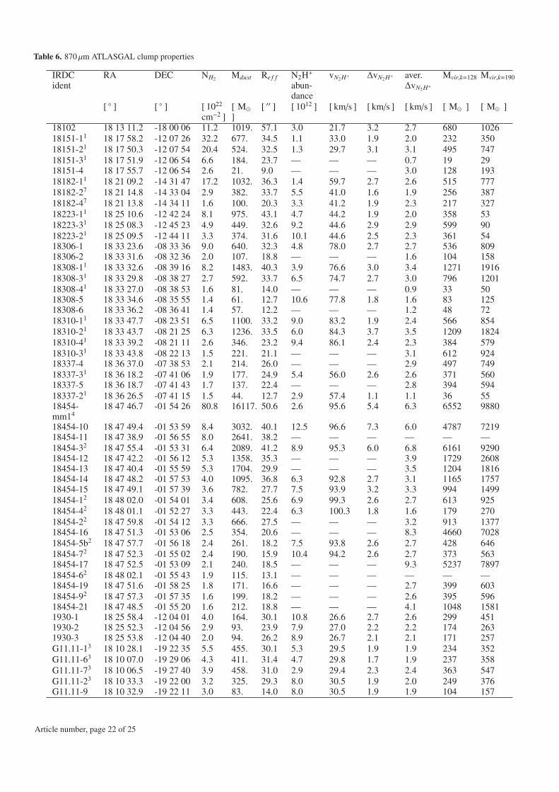
To identify emission peaks and their connected fluxes in thedust maps we use CLUMPFIND (Williams et al. 1994). Sincewe want to compare our results to the dense gas measured byN2H+, we select a lowest emission contour corresponding to1× 1022 cm−2 (> 6σ for ATLASGAL, > 12σ for SCUBA), or,in the case of ISOSS J20153, 2× 1022 cm−2 (> 3σ). Additionallevels are added in steps of 3σ, see Table 2. All clumps forwhich we mapped the peak position are listed together with theircolumn density and mass in Table 6. For clumps that havecommon names in the literature, we try to adopt their previouslabeling. The clump names and references are given in Table 6as well.

The uncertainties on both the gas column density and massare dominated by the dust properties. The flux calibration of theATLASGAL data is reliable within 15%, and typical peak andclump-integrated fluxes are an order of magnitude larger thanthe rms of the data. The uncertainties on the dust propertiesare difficult to assess, but from comparison to other values (e.g.Hildebrand 1983) or using slightly different parameters withinthe same model (Ossenkopf & Henning 1994) we assume themto be on the order of a factor two. Together with the uncertaintiesfrom the dust temperature, we estimate the total uncertainties onthe column densities to be a factor of ∼ 3. For the gas mass, theuncertainty of the distance of ∼ 0.5 kpc introduces an additionalerror of ∼ 50%. Therefore, the total uncertainty of the gas masswe estimate to be on the order of a factor of five.

2.7. Abundance ratio

For positions where not only dust continuum but also N2H+ hasbeen detected we calculate abundance ratios. With a resolutionof 18′′and 19.2′′, the Nobeyama 45 m data have almost the sameresolution as the ATLASGAL 870 µm data. Therefore we cal-culate the N2H+ abundance ratio by plain division, taking thedifferent beam size into account but not smoothing the data. Tocalculate abundance ratios for sources observed with MOPRA ata resolution of 46′′, we apply a Gaussian smoothing to the dustdata to have both at a common resolution. We then calculatethe N2H+ abundance for the 46′′beam. For the analysis, we onlyconsidered dust measurements in the Gaussian smoothed imagesabove 3σ.



3. Morphology of the dense gas

In the following section we concentrate on the N2H+ observa-tions. First we compare the N2H+ to the cold dust distribu-tion as measured by ATLASGAL and put it in context with thePACS 70 µm measurements. Then we describe the velocity andlinewidth distribution of the dense gas.

3.1. Comparing integrated N2H+ and dust continuumemission

The left panels of Fig. 1 through Fig. 4 display the PACS 70 µmmaps with the long-wavelength dust continuum contours on top,the second left panel is the N2H+ column density. They clearlyshow that the N2H+ detection and column density agrees in gen-eral with the measured dense gas emission, almost independentof the evolutionary state of the clump.

The southern component of IRDC G11.11 appears to be pe-culiar, see Fig. 2. While for the northern component the molecu-lar gas traced by N2H+ agrees quite well with the cold gas tracedby thermal dust emission, both dense gas tracers seem to dis-agree for the southern part. Comparing the brightest peak inthe ATLASGAL data to the column density peak of the N2H+

emission, we find a positional difference of 37′′, which is on theorder of the beam size. Since the northern and southern compo-nent have been observed independently, a pointing error couldexplain the offset. However, before and in between the OTF ob-servations we checked the pointing and the offset is considerablylarger than the anticipated pointing uncertainty. Therefore, wecannot explain the spatial offset of the southern map well.

For IRDC 18182, the bright north-western component is con-nected to IRAS 18182-1433 at a velocity of 59.1 km/s (Bronf-man et al. 1996) and a distance of 4.5 kpc (Faúndez et al. 2004).Instead, the region of interest is the IRDC in the south-east ata distance of 3.44 kpc with a velocity of 41 km/s (Beuther et al.2002a; Sridharan et al. 2005).

IRDC 18308 has been selected within this sample for its in-frared dark cloud north of the HMPO IRAS 18308-0841. How-ever, at its distance of 4.4 kpc we do not detect the N2H+ emis-sion from the IRDC with the velocity resolution of 0.2 km/s. Toovercome the sensitivity issue we smoothed the velocity reso-lution to 0.4 km/s and then can trace the dense gas of the IRDCwithin IRDC 18308. For IRDC 18306 the situation is similar, wetrace the HMPO, but not the IRDC. However, even with a ve-locity resolution of only 0.4 km/s we cannot detect N2H+ fromthe IRDC. Therefore, we exclude IRDC 18306 from the discus-sion and show its dense gas properties in the appendix A.2. Toget a better picture of the different regions we display in Fig. 1through Fig. 4 the results from the smoothed maps, where help-ful. However, because the coverage for many clumps is sufficientin the higher resolution data, we used the 0.2 km/s data to do ouranalysis.

The total gas peak column densities over the 19.2′′APEX870 µm beam as given in Table 6 range from 1.4× 1022 cm−2

to 8× 1023 cm−2, and the median averaged peak column den-sity of clumps that have been mapped is 2.6× 1022 cm−2. Ifwe consider only clumps for which the peak position has adetected N2H+ signal, the median averaged peak column den-sity becomes 3.0× 1022 cm−2. For the lower limit one needsto keep in mind that we require a minimum column densitythreshold of 1.0× 1022 cm−2 for a clump to be detected. Theupper limit is set by IRDC 18454-mm1 (adopted from W43-mm1, Motte et al. 2003; Beuther et al. 2012), the brightest clumpwithin IRDC 18454 and a well known site of massive star forma-

tion. All other clumps with peak column densities larger than1× 1023 cm−2 (IRDC 18151-1, IRDC 18182-1, and G 28.34-2)host evolved cores and could be warmer than 20 K. However,to calculate the column densities we assume a constant aver-age dense gas temperature of 20 K. While this is appropriate formost IRDCs in this sample with ongoing early star formation (cf.point sources in Ragan et al. 2012a), using a higher temperaturewould decrease their peak column densities. With the exceptionof W43-mm1, the upper limit of column densities found withinour survey’s sources then becomes ∼ 1× 1023 cm−2 on scales ofthe beam size.

3.2. N2H+ abundance

In order to study the details of the correlation between the densegas and the related N2H+ column density, Fig. 5 shows the pixel-by-pixel correlation between the N2H+ abundance ratio versusthe flux ratio between the Herschel 160 µm and 250 µm bands.One should keep in mind that, as explained in Sect. 2.7, theabundance ratio refers to different beam sizes, dependent on thetelescope that has been used for the observations. The flux ratioof the two PACS bands, or color temperature, can be consideredas a proxy of the dust temperature. For higher temperatures, thepeak of the SED moves to shorter wavelengths, the 160 µm be-comes stronger compared to the 250 µm flux. Therefore, highertemperatures have higher far-IR flux ratios. However, in orderto derive proper temperatures, a pixel by pixel SED fitting is re-quired, which will be done in an independent paper (Ragan etal., in prep.). A known issue in the context of Herschel dataare the unknown background flux levels. Since we only discusstrends within individual regions, we can safely neglect this prob-lem. However, the flux ratios between the different regions arenot directly comparable.

To allow a comparison between IRDCs and regions that donot show up in extinction, we marked pixels that lie within re-gions of high extinction in green. Those regions were selectedby visually identifying the 70 µm flux levels under which extinc-tion features are observed. As the 70 µm dark regions have nosharp boundaries, the chosen levels are not unambiguous.

Figure 5 shows no strong overall correlation between theN2H+ abundance and the flux ratio. On the one hand,IRDC 18223 is an example where there seems to be a correla-tion between the temperature and the N2H+ abundance. Thehighest abundance ratios are found at far-IR flux ratios of thebulge of the pixel distribution, while toward higher temperaturesthe abundance seems to decrease systematically. On the otherhand, in G11.11 the N2H+ abundance varies over two orders ofmagnitude, but shows no correlation with the far-IR flux ratio.For example in G11.11 and G28.34, there seems to be a trendthat the N2H+ abundances become even larger toward the edgesof our N2H+ mapping. However, in these regions we are limitedby the sensitivity of our dust measurements.

Marked by an ’X’ in Fig. 5 are the pixels containing PACSpoint sources. In addition, we distinguish between sources thathave only been detected at 70 µm and longwards, MIPS-darksources, and PACS sources that have a 24 µm counter part,MIPS-bright sources. If the 24 µm image is saturated at the givenposition, sources are considered as MIPS-bright as well. Fromthe figure it can be seen that most embedded PACS sources haveN2H+ abundance ratios below 1× 10−9. However, there seems tobe no correlation between the dust temperature on scales of thebeam size and the presence of embedded PACS point-sources.


18h25m 04s12s

RA (J2000)

48'

46'

44'

-12°42'

De

c (

J20

00

)

IRDC 1 8 2 2 3

PACS 70µm

1 pc

1

3

2

18h25m 04s12s

RA (J2000)

logarithm ic scaling

N2H + CD / [ cm 2 ]

0.05 0.10 0.20 0.50 1.00

1e14

18h25m 04s12s

RA (J2000)

N2H + velo / [ km /s ]

44 45

18h25m 04s12s

RA (J2000)

N2H +∆ v / [ km /s ]

0.5 2.0 3.5

18h33m36s44s52sRA (J2000)

25'

24'

23'

22'

21'

-8°20'

Dec (J2000)

IRDC 18310

1 pc

1

24

3

18h33m36s44s52sRA (J2000)

0.5 1.5 3.0 5.0

1e13

18h33m36s44s52sRA (J2000)

83.0 84.5 86.0

18h33m36s44s52sRA (J2000)

0.5 2.0 3.5

18h47m44s52s48m00sRA (J2000)

58'

57'

56'

55'

54'

53'

-1°52'

Dec (J2000)

IRDC 18454

1 pc

mm110

11

3

1213

1415

1

4

2

16

5b

7

17

6

19

9

21

18h47m44s52s48m00sRA (J2000)

0.5 1.0

1e14

18h47m44s52s48m00sRA (J2000)

93.0 95.3 97.6 101.0

18h47m44s52s48m00sRA (J2000)

1 3 5

Fig. 1. Parameter maps of the regions IRDC 18223, IRDC 18310, and IRDC 18454 mapped with the Nobeyama 45 m telescope, at top, middle,and bottom panel, respectively. The left panel of each row are the PACS 70 µm maps with the PACS point sources detected by Ragan et al.(2012a) indicated by red circles, the blue numbers refer to the sub-mm continuum peaks as given in Table 6. The second panel displays the N2H+

column density derived from fitting the full N2H+ hyperfine structure. The third and fourth panels show the corresponding velocity and linewidth(FWHM) of each fit. For IRDC 18223, and IRDC 18310 the contours from ATLASGAL 870 µm are plotted with the lowest level representing0.31 Jy, and continue in steps of 0.3 Jy. The contour levels for IRDC 18454 are logarithmically spaced, with 10 levels between 0.31 Jy and 31 Jy.The column density scale of IRDC 18223 is logarithmic. The arrow in the fourth panel of IRDC 18223 is taken from Fig. 4 of Fallscheer et al.(2009), indicating the outflow direction.



18h10m00s12s24s36sRA (J2000)

30'

27'

24'

-19°21'

De

c (J

20

00

)

G11.11

PACS 70µm

1 pc

1

67

2

9

10

11

12

13

14

15

16

17

18

19

20

21

22

23

18h10m00s12s24s36sRA (J2000)

N2H+ CD / [ cm−2 ]

0.5 2.0

1e13

18h10m00s12s24s36sRA (J2000)

N2H+ velo / [ km/s ]

28.5 30.0 31.5

18h10m00s12s24s36sRA (J2000)

N2H+ ∆v / [ km/s ]

0.5 2.0

18h17m36s44s

RA (J2000)

51'

50'

49'

-15°48'

Dec (J2000)

G15.05

1 pc

18h17m36s44s

RA (J2000)

3 7

1e12

18h17m36s44s

RA (J2000)

29.5 30.5

18h17m36s44s

RA (J2000)

0.5 1.5

18h13m06s12s18sRA (J2000)

01'

-18°00'

59'

-17°58'

Dec (J2000)

IRDC 18102

1 pc

18h13m06s12s18sRA (J2000)

0.5 1.0 2.0

1e13

18h13m06s12s18sRA (J2000)

21.5 22.0

18h13m06s12s18sRA (J2000)

0.5 2.0

Fig. 2. Parameter maps of the regions G11.11, G15.05, and IRDC 18102, mapped with the MOPRA telescope. The left panel of each row are thePACS 70 µm maps with the PACS point sources detected by Ragan et al. (2012a) indicated by red circles, the blue numbers refer to the sub-mmcontinuum peaks as given in Table 6. The second panel displays the N2H+ column density derived from fitting the full N2H+ hyperfine structure.The third and fourth panels show the corresponding velocity and linewidth (FWHM) of each fit. The green contours are from ATLASGAL 870 µmat 0.31 Jy, 0.46 Jy, and 0.61 Jy, continuing in steps of 0.3 Jy. The velocity resolution in the G15.05 map is smoothed to 0.4 km/s to improve thesignal to noise and increase the number of detected N2H+ positions.

3.3. The large scale velocity structure of clumps andfilaments

The velocity structure of the N2H+ gas is shown in the third panel(second from right) of Fig. 1 to Fig. 4. As explained in Sect.2.5, we fit a single N2H+ hyperfine structure to every pixel anddisplay the resulting peak velocity.

The south-eastern region in the map of IRDC 18182 is theIRDC in the EPoS sample. It already had been known that IRAS

18182-1433, originally targeted by Beuther et al. (2002a), andthe IRDC have different velocities and therefore are spatially dis-tinct. All other sources mapped show velocity variations of onlya few km/s and are therefore coherent structures.

The source with the largest spread in velocity isIRDC 18454 /W43. The mapped regions in the west, beyondW43-mm1 toward W43-main (which has not been mapped),have the lowest velocities at below 93 km/s, then there is a ve-


18h17m48s54s18m00sRA (J2000)

09'

08'

07'

06'

-12°05'

De

c (J

20

00

)

IRDC 18151

PACS 70µm

1 pc

12

34

18h17m48s54s18m00sRA (J2000)

N2H+ CD / [ cm−2 ]0.5 1.0 2.0

1e13

18h17m48s54s18m00sRA (J2000)


29.5 31.5 33.5

18h17m48s54s18m00sRA (J2000)

N2H+ ∆v / [ km/s ]

0.5 2.0 3.5

18h21m06s12s18sRA (J2000)

35'

34'

33'

32'

-14°31'

Dec (J2000)

IRDC 18182

1 pc

1

2

4

18h21m06s12s18sRA (J2000)

0.5 1.0 2.0

1e13

18h21m06s12s18sRA (J2000)

40.5 41.5

18h21m06s12s18sRA (J2000)

0.5 2.0

18182 N2Hplus

18h33m28s36sRA (J2000)

40'

39'

38'

37'

-8°36'

Dec (J2000)

IRDC 18308

1 pc1

34

5

6

18h33m28s36sRA (J2000)

0.5 1.0 2.0

1e13

18h33m28s36sRA (J2000)

75 76 77

18h33m28s36sRA (J2000)

0.5 2.0 3.5

Fig. 3. Parameter maps of the regions IRDC 18151, IRDC 18182, and IRDC 18308, each mapped with the MOPRA telescope. The left panelof each row are the PACS 70 µm maps with the PACS point sources detected by Ragan et al. (2012a) indicated by red circles, the blue numbersrefer to the sub-mm continuum peaks as given in Table 6. The second panel displays the N2H+ column density derived from fitting the full N2H+

hyperfine structure. The third and fourth panels show the corresponding velocity and linewidth (FWHM) of each fit. The green contours are fromATLASGAL 870 µm at 0.31 Jy, 0.46 Jy, and 0.61 Jy, continuing in steps of 0.3 Jy. For IRDC 18151 the contours are MAMBO 1.2 mm observations,starting at 60 mJy in steps of 60 mJy. In all three maps the velocity resolution is smoothed to 0.4 km/s.

locity gradient across W43-MM1 ending east at 97.4 km/s, andin the very south there are two clumps at 100 km/s. However,the velocity map has been derived fitting a single N2H+ hyper-fine structure to each spectrum. Beuther & Sridharan (2007) andBeuther et al. (2012) have shown that, at least at high spectraland spatial resolution, clump IRDC 18454-1 has two velocitycomponents seperated by about 2 km/s. Trying to fit each clumppeak position with two N2H+ hyperfine structures, we find thatfor six continuum peaks, the N2H+ spectrum is better fitted bytwo independent components. For simplicity, we do not include

the additional velocity component found towards IRDC 18454 at∼ 50 km/s (Nguyen Luong et al. 2011).

While a more detailed description of the double line fits arepresented in Sect. 3.4, we here want to note that the mapped linevelocity is representing either a single component if one is muchbrighter than the other, or an average velocity of both. Therefore,the uncertainties for IRDC 18454 are significantly larger than forthe other regions. Nevertheless, the large-scale velocity gradientis no artifact but is evident in the individual spectra.



18h25m52s26m00sRA (J2000)

07'

06'

05'

04'

-12°03'

Dec (J2000)

G19.30

PACS 70µm

1 pc

1

23

18h25m52s26m00sRA (J2000)

N2H+ CD / [ cm−2 ]

0.5 2.0

1e13

18h25m52s26m00sRA (J2000)


26.5 27.5

18h25m52s26m00sRA (J2000)

N2H+ ∆v / [ km/s ]

0.5 2.0

18h42m40s48s56sRA (J2000)

04'

02'

-4°00'

-3°58'

Dec (J2000)

G28.34

1 pc

2

3

1

45

6

7

8

910

18h42m40s48s56sRA (J2000)

0.5 1.5 3.0

1e13

18h42m40s48s56sRA (J2000)

77.5 79.5 81.5

18h42m40s48s56sRA (J2000)

0.5 2.0 3.5

19h21m30s40s50sRA (J2000)

+13°47'

48'

49'

50'

51'

52'

53'

Dec (J2000)

G48.66

1 pc

19h21m30s40s50sRA (J2000)

0.2 0.5 1.0

1e13

19h21m30s40s50sRA (J2000)

33.5 34.5

19h21m30s40s50sRA (J2000)

0.5 1.5

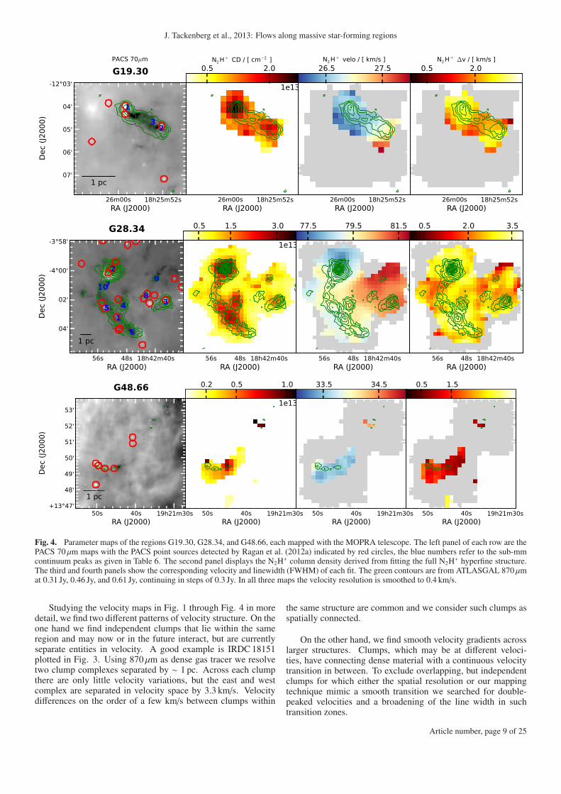
Fig. 4. Parameter maps of the regions G19.30, G28.34, and G48.66, each mapped with the MOPRA telescope. The left panel of each row are thePACS 70 µm maps with the PACS point sources detected by Ragan et al. (2012a) indicated by red circles, the blue numbers refer to the sub-mmcontinuum peaks as given in Table 6. The second panel displays the N2H+ column density derived from fitting the full N2H+ hyperfine structure.The third and fourth panels show the corresponding velocity and linewidth (FWHM) of each fit. The green contours are from ATLASGAL 870 µmat 0.31 Jy, 0.46 Jy, and 0.61 Jy, continuing in steps of 0.3 Jy. In all three maps the velocity resolution is smoothed to 0.4 km/s.

Studying the velocity maps in Fig. 1 through Fig. 4 in moredetail, we find two different patterns of velocity structure. On theone hand we find independent clumps that lie within the sameregion and may now or in the future interact, but are currentlyseparate entities in velocity. A good example is IRDC 18151plotted in Fig. 3. Using 870 µm as dense gas tracer we resolvetwo clump complexes separated by ∼ 1 pc. Across each clumpthere are only little velocity variations, but the east and westcomplex are separated in velocity space by 3.3 km/s. Velocitydifferences on the order of a few km/s between clumps within

the same structure are common and we consider such clumps asspatially connected.

On the other hand, we find smooth velocity gradients acrosslarger structures. Clumps, which may be at different veloci-ties, have connecting dense material with a continuous velocitytransition in between. To exclude overlapping, but independentclumps for which either the spatial resolution or our mappingtechnique mimic a smooth transition we searched for double-peaked velocities and a broadening of the line width in suchtransition zones.


Fig. 5. Plotted is the N2H+ abundance ratio over the color index between 160 µm and 250 µm. Marked by green dots are pixels that lie withinIRDCs. Overplotted with red Xs are all PACS sources that have been mapped. Blue crosses also have a 24 µm detection, while the light blue dotsrepresent source that are saturated at 24 µm. The uncertainties given for IRDC 18223 are representative for all regions.

The velocity maps of G15.05, IRDC 18102, IRDC 18151,IRDC 18182, and G48.66, Fig. 1, Fig. 2, Fig. 3, and Fig. 4,immediately reveal that those complexes have no velocity gradi-ents in the gas above our detection limits given in Table 7 andtherefore are of the first type. A summary of the clump classifi-cation is given in Table 7.

For IRDC 18310, shown in Fig. 1, the velocity map showsthat the IRAS source in the south has a velocity of 83.2 km/s(see also Table 6), while the northern complex has larger ve-locities. Nevertheless, the velocity spread suggests an associ-ation between both clumps. In addition, the northern compo-nent itself has different velocities toward the east and south,with 86.1 km/s and 84.3 km/s. In between there is a short tran-sition zone with an spatially associated increase in the linewidth(see very right panel of Fig. 1). The increase in linewidth sug-gests that there is indeed an overlap of two independent velocitycomponents, rather than a large scale velocity transition. Us-ing the unsmoothed Nobeyama image at an velocity resolutionof 0.2 km/s, the spectra suggest two independent components.Therefore, IRDC 18310 consists of three clumps, each showingno resolved velocity structure.

IRDC 18151, shown in Fig. 3, consists of two clumps atdifferent velocities. While the velocities of the western clumpagree within 0.5 km/s, the eastern clump has a velocity gradientfrom the south-east to the north-west with a change in veloc-ity of more than 1 km/s. However, at the velocity resolution of0.2 km/s we do not detect the lower column density transition re-gion and cannot exclude a smooth transition across both clumps.To overcome the sensitivity issue we smooth the N2H+ data toa resolution of 0.4 km/s. Still, only a single pixel with a goodenough signal to noise ratio connects both dense gas clumps. Aswe will discuss in Sect. 4.4, the found pattern does not suggesta smooth transition.

For IRDC 18454, IRDC 18308, G11.11, G19.30, and G28.34we find smooth velocity gradients. One of the largest smooth ve-locity gradients of the sample is found toward the southern partof IRDC 18308, across the HMPO. Although there is an increasein the linewidth map, even in the unsmoothed higher resolutiondata we cannot find two independent components. Over 3.2 pcthe velocity changes by 2.4 km/s, resulting in a velocity gradientof 0.8 km/s /pc. The change in velocity is parallel to the elonga-tion of the ATLASGAL 870 µm emission.



Table 7. Selected clump properties.

Source Velocitygradient

Doublecomponent

Increase in ∆vtowards peak

Decrease in ∆vtowards peak

Outflowdominated ∆v

Flow alongfilament

IRDC 18223 1 18223-2 18223-118223-3

18223-13

18223-3?

IRDC 18310 18310-4IRDC 18454 ?IRDC 18102 18102 18102

IRDC 18151 18151-2 18151-1 18151-23

IRDC 18182 18182-1 18182-2IRDC 18308 18308-1

IRDC 19.30 G19.30-1 G19.30-2 G19.30-13

G19.30-23

IRDC 11.11 G11.11-1G11.11-2

G11.11-12

IRDC 15.05 G15.053

IRDC 28.34 G28.34-1G28.34-2

G28.34-10 ?

IRDC 48.66 G48.663

The columns are as follows: full region name; flag indicating whether we find a smooth velocity gradient along the region; flag indicating thepresence of resolved independent velocity components along a line of sight; two columns for clumps for which we find a clear increase in

linewidth towards the center and towards the edge clumps, respectively; flag indicating that the velocity profile is consistent with flows along thefilament. Notes: (1) For 18223 we find several velocity gradients, both along and perpendicular to the filament. (2) The angle between theoutflow and the linewidth broadening does not match exactly. (3) Indirect evidence for outflow (mainly from SiO), but the direction of the

outflow is unknown.

The velocity gradient in the northern part of G11.11 is simi-larly clear as it is for IRDC 18308 and is parallel to the extinctionof G11.11. While the very southern tip of the northern filamentis at a slightly different velocity, up north it has an almost con-stant velocity up to the point G11.11-1 and then shows a strongbut smooth gradient beyond.

As mentioned before, if considering the length and change invelocity only, the samples largest velocity gradient is found forIRDC 18454. Over a length of 8.4 pc the gradient is 0.9 km/s /pc.However, in between the two endpoints the velocity is not in-creasing monotonically.

IRDC 18223 shows significant changes in the velocity field,but is not listed among the clumps with smooth velocity gra-dients. The changes of the velocity are on 0.5 pc - 1 pc scalesand show no clear pattern. Nevertheless, at the given velocityresolution of 0.5 km/s we do not find overlapping independentN2H+ components. Therefore, all the gas on the scales we traceseems to be connected. It is worth noting that the two south-ern clumps, IRDC 18223-2 and IRDC 18223-3, have a gradientalong the short axis of the filament, which might be interpretedas rotation. Velocities in the east are larger than the velocitiesin the west. In contrast, although less well mapped, the IRASsource in the north, IRDC 18223-1, has a velocity gradient alongthe short filament axis, too, but in opposite direction; velocitiesin the west are larger than in east.

For G13.90, IRDC 18385, IRDC 18306, and IRDC 18337 welack the sensitivity to draw a conclusion. While IRDC 18385,and IRDC 18306 are not reasonable mapped at all, for G13.90and IRDC 18337 we map the main emission structures, but withthe given sensitivity we do not trace the gas in between the denseclumps. In both sources, the detected clumps have differingvelocities, with a gradient accross the clumps in IRDC 18337.However, since we do not trace the gas in between the denseclumps, we cannot assess whether the velocity transitions aresmooth, or the clumps have no connection in velocity space.

3.4. The N2H+ linewidth in context of young PACS sourcesand column density peaks

The right panel of Fig. 1 to Fig. 4 show the fittedlinewidth (FWHM) for the mapped regions. The distributionof the linewidth is very different for each region and den-sity peak. While it increases toward some of the sub-mmpeaks (e.g. IRDC 18102, IRDC 18182-1), for others the peakof the linewidth is on the edge of the sub-mm clumps (e.g.IRDC 18223-1, IRDC 18223-3, G19.30). The IRDCs for whichwe detect N2H+ and that have no embedded/detected PACSsource often have a smaller linewidth than other clumps of thesame region with embedded protostars.

A brief description of the linewidth distribution of each re-gion is given in the Appendix A. In the following we discuss afew interesting/notable examples.

While the linewidth in IRDC 18223 increases towardIRDC 18223-2 significantly, the linewidth toward IRDC 18223-1, a well studied HMPO (Sakai et al. 2010), and IRDC 18223-3,an object known to drive a powerful outflow (Beuther & Sridha-ran 2007; Fallscheer et al. 2009), increases toward the edges ofthe dust continuum. Compared to other regions of IRDC 18223,the linewidth at IRDC 18223-3 is elevated, but it broadens fur-ther toward the north-west. This aligns very well with the out-flow found by Fallscheer et al. (2009) and can be explained byit (for the outflow direction see the first row of Fig. 1, rightpanel). IRDC 18223-1 was originally identified as IRAS 18223-1243 and is bright at IR wavelengths (down to K band). How-ever, typical tracers of ongoing high-mass star formation such ascm emission, water and methanol masers, or SiO tracing shocksare not detected (Sridharan et al. 2002; Sakai et al. 2010). Onlythe CO line wings found by Sridharan et al. (2002) are indicativeof outflows, which could explain the bipolar broadening of theN2H+ linewidth well. Nevertheless, despite its prominence at IRwavelengths and with the luminosity of the PACS point sourceat its peak of 2000 L⊙ (point source 8 in Ragan et al. 2012a), thelinewidths at the continuum peak are not exceptional within this


Fig. 6. Spectra of IRDC 18454-4 Beuther & Sridharan (2007); Beutheret al. (2012). While the dashed line shows the single component fit withthe fitting parameters to the right, the solid line is the two component fitwith its fitting parameters to the left. The given residuals are the resultsof the minimize task in CLASS.

region. In contrast, although IRDC 18223-2 is detected at nearIR wavelengths as well and the PACS point source at its centerhas a luminosity of only 200 L⊙, the linewidth is 2.5 kms/s com-pared to 1.9 km/s for IRDC 18223-1. Since Beuther & Sridharan(2007) find no SiO toward IRDC 18223-1/2 we exclude a strongoutflow, and the reason for the line broadening is not clear at all.However, IRDC 18223-2 has not been addressed in such greatdetail and we cannot entirely exclude an outflow.

We exclude IRDC 18454 from the analysis of the linewidthsince, as already mentioned in Sect. 3.3, we find multiple ve-locity components toward several positions. Figure 6 displaysan example of an N2H+ spectrum that compares a single com-ponent fit to a double component fit. Comparing the residuals ofthe two different fits as calculated by CLASS, for the six clumpsin which we find two independent components the residuals areon average reduced by 30%. As for all two component fits, thelinewidth decreases compared to a single component fit. How-ever, the linewidths are then on average still larger than for theother clumps listed in Table 6.

Similar double velocity component fits toward the peaks areotherwise only possible in G11.11. Here, eight of the clumpsare fit better by two independent N2H+ components. However,different from IRDC 18454 the linewidth of the two componentsbecome on average smaller than the linewidth of other clumpsin the sample. In addition, the improvement of the residuals isonly 20%. Therefore it is unclear whether two independent com-ponents are present or the fit is simply improved because of thelarger number of free parameters. However, a systematic studyof the multiple components is beyond the scope of this paper.

For G13.90, IRDC 18385, IRDC 18306, and IRDC 18337 themapped areas are not sufficient to draw conclusions.

Similar to Fig. 5, Fig. 7 shows the relation between thelinewidth (FWHM) of N2H+ and the color index. Since the colorindex is a proxy of the temperature, a correlation between bothquantities could have been expected. However, we do not seeany correlation. Figure 8 plots the N2H+ linewidth versus the H2

column density, but we find no correlation.In the context of the linewidth and dust mass, the virial anal-

ysis can be used to understand whether structures are gravita-tionally bound or are transient structures. Following MacLarenet al. (1988), we calculate the virial mass of our clumps viaMvir = k R∆v2. For the clump radius R we use the effective ra-dius calculated by CLUMPFIND. The geometrical parameter kdepends on the density distribution, with k= 190 for ρ∼ r−1, and

Fig. 9. Top panel: Plot of the virial mass derived from the N2H+

linewidth over the gas mass. The virial mass assumes a geometricalparameter of k=158, which is intermediate between k=126 for 1/ρ2 andk=190 for 1/ρ. While the black dots indicate clumps without a PACSpoint source inside, the asterisks represent clumps with a PACS pointsource. Marked by green and red squares are the clumps of G28.34,with green boxes representing clumps in global infall, and red boxesrepresenting clumps with signatures of outwards moving gas (for detailssee Tackenberg et al., submitted). The solid line indicates unity. Lowerpanel: Histogram of the virial parameter α. While the black histogramrepresents the full sample, the red and green histogram is the subset ofclumps with and without PACS point source, respectively.

k= 126 for ρ∼ r−2. Beuther et al. (2002a), Hatchell & van derTak (2003), and Peretto et al. (2006) find typical density distri-butions in sites of massive star formation of ρ ∝ rα with α∼ -1.6,in between both parameters. While we list the virial mass forboth parameters in Table 6, we use the intermediate value ofk= 158 in Fig. 9.

The α parameter as defined in Bertoldi & McKee (1992) isthe ratio of the internal kinetic energy and the gravitational en-ergy. However, their virial parameter as defined in Eqn. 2.8a of

Bertoldi & McKee (1992) (α= 5σ2RGM

) without further geometri-cal parameter resembles a spherical distribution of constant den-sity. Due to the geometrical correction factor we apply to the



Fig. 7. Plot of the N2H+ linewidth versus the color index for the 160 µm over the 250 µm band. Marked by green dots are pixels that lie withinIRDCs. Overplotted with red Xs are all PACS sources that have been mapped. Blue dots also have a 24 µm detection, while the pale blue dotsrepresent source that are saturated at 24 µm. The uncertainties given for IRDC 18223 are representative for all regions. For IRDC 18454 thelinewidths have been multiplied by a factor of 0.5 in order to fit the data points into the plotting range.

mass calculations, the presented virial parameters are smaller bya factor of 1.32. A histogram of the virial parameter is plotted inFig. 9.

If we assume the error on our linewidth to be less than 15%,the uncertainties of the calculated virial mass are mainly deter-mined by the geometrical parameter k. The actual error on thegiven virial masses is significantly larger since the calculationneglects all physical effects but gravity and thermal motions (ki-netic energy). However, for the conceptual quantity we can ne-glect these effects and estimate the error to be ∼ 50%.

4. Discussion of N2H+ dense gas properties

In the following, we will discuss the kinematic properties ofsources we mapped in N2H+, as described above.

4.1. Dense clumps and cores

The clump masses in the range of several tens of M⊙ to a fewthousands of M⊙ show that most regions have the potential to

form massive stars in the future, or show signs of ongoing high-mass star formation. One should keep in mind that the listedpeak column densities are averaged over the beam. As it hasbeen shown by Vasyunina et al. (2009) assuming an artifical r−1

density profile, true peak column densities are larger by a factorof 20 to 40. This is in agreement with interferometric observa-tions of clumps within our sample (Beuther et al. 2005, 2006;Fallscheer et al. 2011). Therefore, all peak column densities be-come larger than 3× 1023 cm−2, or 1 g/cm2. This reinforces theview that the mapped clumps are capable of forming massivestars. The high column densities are also in agreement with thedetection of N2H+ as high density gas tracer.

4.2. Abundance ratios

In order to understand why the abundance of N2H+ is expectedto vary with embedded sources or temperature, one needs tounderstand the formation mechanism. The formation of N2H+

works via H+3

which also builds the basis for the formation ofHCO+ from CO. Due to the high abundance of CO in cold dense


Fig. 8. Plot of the N2H+ linewidth versus the dust column density. Marked by green dots are pixels that lie within IRDCs. Overplotted with redXs are all PACS sources that have been mapped. Blue dots also have a 24 µm detection, while the pale blue dots represent source that are saturatedat 24 µm. The uncertainties given for IRDC 18223 are representative for all regions. For IRDC 18454 the linewidths have been multiplied by afactor of 0.5 in order to fit the data points into the plotting range.

clouds, the production of HCO+ is initially dominant and con-sumes all H+

3. However, if during cloud contraction the temper-

atures become cold enough for CO to freeze out, N2H+ can beproduced more efficiently and eventually becomes more abun-dant than HCO+. The situation changes again when CO becomesreleased from the grains either due to heating or due to shocks.The CO destroys the N2H+ and forms HCO+ instead, makingHCO+ more abundant again. (For a more detailed discussion seeJørgensen et al. 2004.)

In summary, the early, (more diffuse) cloud phase is domi-nated by HCO+, while the quiet dense clumps should be domi-nated by N2H+. With the onset of star formation, HCO+ is be-coming dominant again.

The EPoS sample mainly has been selected to cover regionsof ongoing, but early star formation. For this N2H+ line survey,we selected regions covering all evolutionary stages. Many ofthem have both infrared quiet regions at the wavelengths rangecovered previous to Herschel as well as well known and lumi-nous IRAS sources. Together with the Herschel data, hardly anyregion of high column density is genuine infrared dark.

As a result of both the N2H+ evolution and the broad rangeof evolutionary stages covered, we expect a large range of N2H+

abundance ratios. As it has been discussed in Sect. 3.2, Fig.5 shows the correlation between the N2H+ abundance and the160 µm to 250 µm flux ratio as a proxy of the temperature. Forall regions, the bulk of all pixels has N2H+ abundances ratiosof 1× 10−9. That is in good agreement with earlier studies ofhigh-mass star-forming regions (Vasyunina et al. 2011, and ref-erences therein). At the same time several regions (e.g. G11.11,G28.34, IRDC 18454) show abundance variations of two ordersof magnitude. While this is a result of the various evolutionarystages within each region, it is worth noting that it seems not tobe correlated to the flux ratio of 160 µm over 250 µm.

In order to correlate some areas with an evolutionary stage,in Fig. 5 we differentiate regions that show up in extinction at70 µm by green dots. As Fig. 5 shows, these regions are amongthe coldest within each region. Nevertheless, high N2H+ abun-dances are found not only in IRDCs or cold regions. In contrastto IRDC pixels which mark the earliest and coldest evolutionarystages, the PACS only sources mark regions in which star for-



mation is about to start (red), and the MIPS bright PACS sourcesindicate ongoing star formation (blue). All pixels connected toa PACS source have low N2H+ abundances. Whether this is dueto an increase in temperature or probably because of shocks isunclear.

It has been shown in Ragan et al. (2012a) that sources withdetected 24 µm counterpart are on average warmer, more lumi-nous, and more massive and therefore a 24 µm counterpart is in-dicative of a more evolved source. Nevertheless, the PACS coreproperties in Ragan et al. (2012a) show a large overlap betweenMIPS bright and dark sources. Therefore, one cannot draw aclear conclusion on the evolutionary stage (temperature, lumi-nosity, or mass) based on a 24 µm detection alone. This easilyexplains exceptions as e.g. in G11.11.

4.3. Signatures of overlapping dense cores within clumps

As we describe in Sect. 3.3, we find two independent veloc-ity components toward six of the IRDC 18454 continuum peaks,as well as 7 clumps in G11.11 with double peaked N2H+ lines.The two components have velocity offsets of only a few km/s.Since the hyperfine structure of N2H+ includes an optically thincomponent, we can exclude opacity and self absorption effects,a common feature in dense star-forming regions. The two inde-pendent velocity components within IRDC 18454 have alreadybeen reported by Beuther & Sridharan (2007); Beuther et al.(2012), and Ragan et al. (in prep.) find multiple velocity com-ponents toward G11.11. Combining our N2H+ Nobeyama datawith PdBI observations at ∼ 4′′, Beuther et al. (2013) revealmultiple independent velocity components toward IRDC 18310-4. These are not resolved within the Nobeyama data alone atthe spatial resolution of 18′′. Similar multi-component velocitysignatures have been found in high spatial resolution images ofdense cores in Cygnus-X (Csengeri et al. 2011a,b), and towardIRDCs by Bihr et al. (subm.). Therefore, it seems to be a com-mon feature in high-mass star-forming regions.

Using radiative transfer calculations of collapsing high-massstar-forming regions, Smith et al. (2013) show that such doublepeaked line profiles may be produced by the superposition of in-falling dense cores. Therefore, in high-resolution studies, whichfilter out the large scale emission, multiple cores along the line-of-sight can be detected. However, comparing our beam sizes of∼ 0.5 pc for IRDC 18454 and ∼ 0.8 pc for G11.11 to typical sizesof cores below 0.1 pc, the larger-scale clump gas should may bedominating our signal. Therefore it is clear that multiple velocitycomponents due to cores are more likely to be identified in highspatial resolution imaging. While IRDC 18454 is at the inter-section of the spiral arm and the Galactic bar, and therefore ex-ceptional in many aspects, G11.11 is likely a more typical high-mass star-forming region, similar to what has been simulated bySmith et al. (2009) and Smith et al. (2013). If the double peakedline profiles originate from two dense cores within our beam, assuggested by Smith et al. (2013), the cores within G11.11 wouldneed to be extremely dense or large. Instead, it seems more re-alistic that we detect the gas of the clump as one velocity com-ponent, and the second component is produced by an embeddedsingle core of high density contrast moving relative to its parentclump. For IRDC 18454 we find double velocity spectra even in-between the peak positions. This suggests that the componentsare coming from two overlapping sheets, close in velocity. It isunclear whether these sheets are interacting or not.

4.4. Accretion flows along filaments?

In Sect. 3.3 we presented the velocity structure of the 16 ob-served high-mass star-forming regions. As we described, 5complexes have no velocity structure, while 6 regions havesmooth large scale velocity gradients. The velocity structure ofIRDC 18223 is more complex and does not fit into either of thesecategories. For 4 regions we lack the sensitivity to draw a con-clusion.

Despite the two general appearances, the large scale veloc-ity structure of the clumps is very diverse. In general, structureslarger than 1 pc usually show some velocity fluctuations. Thesecan be either steady and smooth, or pointing to separate entities.It is worth noting that the physical resolution of the N2H+ ob-servations ranges from 0.1 pc to 1.0 pc, with an average of 0.3 pcfor the 18′′Nobeyama beam, and 0.7 pc for the 46′′with MO-PRA. Therefore, we are not able to resolve smaller structures,and the 1 pc limit is observationally set. In fact, velocity fluctua-tions on smaller scales are still likely. However, the observationsshow that on clump scale, some clumps do show gas motions,while others are kinematically more quiescent. High-resolutionstudies, e.g. Ragan et al. (2012b), have proven for some regionsthat on smaller scales gas motions continue.

In order to understand the velocity structure of complexeswith smooth velocity transitions, Figure 10 through Fig. 16 vi-sualize the velocity gradients along given lines. As it hasbeen discussed in Sect. 3.3, our velocity map of IRDC 18151consists of 2 larger structures, IRDC 18151-1 in the east, andIRDC 18151-2 and IRDC 18151-3 in the west. The overallchanges within the eastern and western clump are ∼ 0.5 km/s and∼ 1 km/s, respectively. However, while the velocity cut throughthe eastern clump shows hardly any variation, the western clumphas a noticeable velocity gradient. To detect at least part of thegas at intermediate velocities, we smoothed the N2H+ to a veloc-ity resolution of 0.4 km/s. Figure 12 shows the velocity profileacross both clumps. While the western clump shows a slightvelocity increase toward the east, the eastern clump shows novelocity gradient. Especially, both gradients seem not to match,and if they interact dynamically, the transition zone would needto be short. Therefore we conclude that both structures are indi-vidual components, but in the context of other dense gas tracersboth seem to be embedded within the same cloud. If seen froma slightly different angle, the double velocity components dis-cussed in Sect. 4.3 could well originate from such a structure.

4.4.1. Flows along G11.11

A clear smooth transition of the velocity we find toward thenorthern part of G11.11. Shown by the top profile in Fig. 14, be-tween G11.11-1 and G11.11-12, the differences in velocity arebelow 0.5 km/s. Along the profile just south of G11.11-1, thevelocity starts to increase, with higher velocities toward G11.11-2 and beyond. On the other hand, the profiles perpendicular tothe filament, right panel of Fig. 14, have almost constant veloci-ties. Only the profile closest to G11.11-1 has a velocity gradient.However, the filament has a bend right at the position of the pro-file. A profile perpendicular to the actual shape of the IRDCwould have no velocity gradient. Therefore, we conclude thatthe velocity gradient is solely along the filament.

Both Tobin et al. (2012) (observationally), and Smith et al.(2013, numerically), suggest large-scale accretion flows alongfilaments on, and probably producing, central cores. They de-scribe the expected observational signatures for filaments thatare inclined from the plane of the sky. Imagine a cylinder with a


18h25m04s12sRA (J2000)

48'

46'

44'

-12°42'

Dec (J2000)

1

3

2

44 45

44.0 44.5 45.0velo / [ km/s ]

44.0

44.5

45.0

velo / [ km

/s ]

Fig. 10. Profile of the N2H+ velocity of IRDC 18223. The left panelshows the velocity map with contours from ATLASGAL superimposed(see also Fig. 1). The right and top panels show the velocity cuts alongthe lines marked on the velocity map. The stars mark the velocities ofthe clump peaks.

central core, and material flowing onto the core from both sidesat a constant velocity. For simplicity and without loss of gen-erality, we put the central core at rest. Then, on each side ofthe central object the gas has a constant velocity along the fila-ment. Since the gas is flowing in from both sides onto the core,a constant velocity is observed for both directions. The angle ofthe filament to the line-of-sight determines the observed velocitycomponent. While Tobin et al. (2012) accounts for a gravitation-ally accelerated gas flow which should have a velocity jump atits center, the synthetical observations of high-mass star-formingregions performed by Smith et al. (2013) have a smooth tran-sition. They also find local velocity variations, connected tosmaller substructures.

Recalling the velocity structure we find for G11.11, our ob-servations could be explained by such accretion flows along thefilament. The filament would need to have an angle such thatthe south-east is further away from us than the north-west. Thealmost constant velocity over ∼ 3 pc would be material movingtoward G11.11-1, the most massive clump in the region. Just be-

18h47m44s52s48m00sRA (J2000)

58'

57'

56'

55'

54'

53'

-1°52'

Dec (J2000)

mm1

10

11

3

1213

1415

1

4

2

16

5b

7

17

6

19

9

21

93.0

95.3

97.6

101.0

93.0

95.3

97.6

101.0

velo / [ km

/s ]

Fig. 11. Profile of the N2H+ velocity of IRDC 18454. The left panelshows the velocity map with contours from ATLASGAL superimposed(see also Fig. 1). The top panel shows the velocity cut along the linemarked on the velocity map. The stars mark the velocities of the clumppeaks.

fore G11.11-1, the velocity starts to increase and we observe thetransition across the clump. Beyond G11.11-1, the gravitationalpotential of G11.11-2, the second most massive clump in this re-gion, accretes material on its own, and accelerates the gas evenfurther beyond the position of G11.11-1.

The scales we trace are an order of magnitude larger thanwhat has been discussed by Smith et al. (2013) and our reso-lution is an order of magnitude worse. Because of the seconddense clump, we do not observe the theoretically predicted pat-tern. The increase in velocity could also be explained by solidbody rotation of part of the filament. Nevertheless, we proposean accretion flow along the filament as a possible explanation forthe observed velocity pattern in G11.11. This view is supportedby the fact that star-formation is most active at the center of thepotential infall.

Consequently, if high-mass star formation is actively ongo-ing within G11.11-1, the material flow along the filament sug-gests continuous feeding of the mass reservoir from which form-ing stars can accrete.

4.4.2. Flows along IRDC 18308

A similar scenario could explain the velocity pattern along theIR dark part of IRDC 18308. The cut along the IRDC endingat the HMPO, see Fig. 13, shows only minor changes in ve-locity across the IRDC of ∼ 2.5 pc length. In the vicinity ofIRDC 18308-1, the velocity changes by almost 1 km/s on a shortphysical scale of only ∼ 0.6 pc. The cut does leave a gap to theHMPO and does not fully close up in velocity. As described in



18h17m52s18m00sRA (J2000)

08'

-12°07'

Dec (J2000)

1

2

34

29.5

31.5

33.5

29.5

31.5

33.5

velo / [ km

/s ]

Fig. 12. Profile of the N2H+ velocity of IRDC 18151. The left panelshows the velocity map with contours from ATLASGAL superimposed(see also Fig. 3). The top panel shows the velocity cut along the linemarked on the velocity map. The stars mark the velocities of the clumppeaks.

18h33m28s36sRA (J2000)

40'

39'

38'

37'

-8°36'

Dec (J2000)

1

3

4

5

6

75

76

77

75

76

77

velo / [ km

/s ]

75 76 77velo / [ km/s ]

Fig. 13. Profile of the N2H+ velocity of IRDC 18308. The left panelshows the velocity map with contours from ATLASGAL superimposed(see also Fig. 3). The top and right panels show the velocity cuts alongthe lines marked on the velocity map. The stars mark the velocities ofthe clump peak.

Sect. 3.3, across the HMPO we find one of the largest velocitygradients in our sample, but the origin is unclear. One possi-ble explanation that would produce a similar velocity profile issolid body rotation. In this picture, the knees at both ends of theprofile would be caused by a transition from solid-body rotationto viscous rotation because of the lower densities in the outer

18h10m16s24s32sRA (J2000)

25'

24'

23'

22'

21'

-19°20'

Dec (J2000)

1

2x

x

x

x

x

x

x

x

x28.5

30.0

31.5

28.5

30.0

31.5

velo / [ km

/s ]

28.5 30.0 31.5velo / [ km/s ]

Fig. 14. Profile of the N2H+ velocity of the northern part of G11.11.The left panel shows the velocity map with contours from ATLASGALsuperimposed (see also Fig. 2). The right and top panels show thevelocity cuts along the lines marked on the velocity map. The starsmark the velocities of the clump peak.

18h25m52s26m00sRA (J2000)

05'

04'

-12°03'

Dec (J2000)

1

2

3

26.5

27.5

26.5

27.5

velo / [ km

/s ]

Fig. 15. Profile of the N2H+ velocity of G19.30. The left panel showsthe velocity map with contours from ATLASGAL superimposed (seealso Fig. 4). The top panel shows the velocity cut along the line markedon the velocity map. The stars mark the velocities of the clump peak.

regions. However, a full explanation would require a combina-tion of hydrodynamic simulations with radiative transfer calcu-lations. This is beyond the scope of this paper.

4.4.3. Flows along G19.30?

In G19.30, along the north-eastern part of the IRDC the velocityis constant over ∼ 1 pc, and then it rises toward its other end.This suggests that the gas is flowing across G19.30-1, at thenorth-eastern end, through G19.30-3 towards G19.30-2. How-


18h42m40s48s56sRA (J2000)

04'

02'

-4°00'

-3°58'

Dec (J2000)

2

3

1

45

6

7

8

9

10

77.5

79.5

81.5

77.5

79.5

81.5

velo / [ km

/s ]

77.5 79.5 81.5velo / [ km/s ]

Fig. 16. Profile of the N2H+ velocity of G28.34. The left panel showsthe velocity map with contours from ATLASGAL superimposed (seealso Fig. 4). The top and right panels show the velocity cuts along thelines marked on the velocity map. The stars mark the velocities of theclump peaks.

ever, G19.30-1 is the most massive clump and therefore is poten-tially building the center of gravity. Therefore, the flow is oppo-site to the gravitational potential. The dust temperatures derivedfor the cores within G19.30 by Ragan et al. (2012a) are higherfor the more massive clump G19.30-1, increasing our uncertain-ties on the mass. Nevertheless, even if we assume the higherdust temperature of 25 K for the whole G19.30-1 clump, and atemperature of 17 K for G19.30-2, both masses become of thesame order. The additional clump G19.30-3 close to G19.30-2,is of similar mass as G19.30-2 and therefore increases the grav-itational potential of the south-western end. Nevertheless, if ourinterpretation of a gas flow along the filament is correct, we donot find evidence that is it driven by gravity. Instead, this ex-ample could be interpreted as indication for a primordial originof the flows, which lead to the formation of the clumps. Sim-ilar as for G11.11, the flows along the filaments within G19.30and IRDC 18308 support the idea that the mass reservoir in high-mass star formation is continuously replenished.

4.4.4. The peculiar case of IRDC 18223

IRDC 18223 is filamentary, but with a more complex velocitystructure than the previously discussed regions. Along the fila-ment the velocity seems to be oscillating. The emission peaksof the southern clumps, IRDC 18223-2 and IRDC 18223-3, areat the same velocity of 44.6 km/s and in between the variationsare minor. The peak of the clump IRDC 18223-1, harboring theHMPO IRAS 18223-1243, has a velocity of 44.2 km/s.

Perpendicular to the filament, we find three extreme veloc-ity gradients, shown in Fig. 10. Although they are not goingdirectly across the dust continuum emission peaks, each seemsto be associated with a clump. A straight forward interpreta-tion would be solid body rotation along the filament axis. How-ever, as mentioned in Sect. 3.3, the two lower profiles indicate

rotation in the opposite direction to the upper most profile. InSect. 3.4 we discuss the possible influence of the powerful out-flow within IRDC 18223-3 on the linewidth distribution. Thesame outflow could also alter the velocity distribution in its di-rect vicinity. Nevertheless, a change in rotation orientation alonga single filament seems counter intuitive. For the massive fila-ment DR21 within Cygnus X, (Schneider et al. 2010) find threevelocity gradients perpendicular to the filament axis, with alter-nating directions. Suggesting turbulent colliding flows as originof the filament, they interprete the velocity pattern as a remnantof the external flow motions.

Within IRDC 18223-3, on scales of 7′′, Fallscheer et al.(2009) find a velocity gradient in N2H+ and CH3OH, a highdensity and shocked gas tracer. They successfully model theCH3OH velocity gradient with a rotating and infalling toroid,significantly larger than massive disk candidates (e.g. Cesa-roni et al. 2005, for a contradictive example see Boley et al.2012). However, the small scale velocity gradient presented inFallscheer et al. (2009) has not only a slightly different orien-tation (by ∼ 45), but is also rotating in the counter directioncompared to the gradient presented in Fig. 10. This implies thatboth gradients are independent and have different origins; thesmall scale infalling toroid is not connecting the large scale en-velope to a possibly even smaller scaled disk. To first order thiscontradicts our previous statement of continuously feed clumps,because in this particular case, the large scale mass reservoir, orenvelope, seems to be disconnected from the embedded HMPO.On the one hand, the velocity gradient seen in the large-scalegas might be confused by the outflow. As we discuss in Sec.4.5.1, there is a clear correlation between the outflow and thelinewidth distribution. Although N2H+ is not known to be com-monly entrained in outflows, a similar correlation between theoutflow and the velocity gradient seems not unlikely and couldexplain the change in velocity. Here we need to emphasize thatthe outflow direction and velocity gradient have an angle of al-most 90. On the other hand, it could well be that the accretionphase of IRDC 18223-3 has already stopped, and the large-scaleenvelope and the inner toroidal structure are decoupled. How-ever, apart from its youth, it is counter-intuitive that the core firstaccreted from a rotating structure, and then developed an internalsource rotating in the opposite direction. Therefore, we cannotoffer a good explanation.

4.4.5. G28.34

A quite large and complicated region is G28.34. Most promi-nent and clear, it has a strong but smooth east to west veloc-ity gradient. Along the velocity cut given in the top panel ofFig. 16, the velocity changes by 2.6 km/s over 7.1 pc. This re-sults in a velocity gradient of 0.4 km/s/pc. The clump emissionpeaks within the south-eastern component of G28.34, namelyG28.34-6, G28.34-1, and G28.34-5, all have the same velocity.However, as the velocity cut along them shows, the velocity ofthe dense gas between them seems to be oscillating, similar asfound for IRDC 18223. Even further north, the emission peaksof G28.34-7, and G28.34-10 are still at the same velocity as themore southern clumps. Only north of those the velocity changesmonotonically to smaller velocities on the order of a parsec.

From the smooth velocity transition from east to west, aswell as the absence of double peaked N2H+ profiles, we con-clude that all dense gas within the region is physically connected.However, to fully explain the observed velocity signatures of thecomplex dense gas morphology in G28.34, again numerical sim-ulations are likely required.



4.4.6. IRDC 18454

The velocity analysis of IRDC 18454 is hampered by the factthat, as discussed in Sect. 4.3, several clumps show two inde-pendent velocity components at their peak position. Therefore,the mapped single velocities can either be the stronger of thetwo components, or an average of both. However, the large scalevelocity gradient in east to west direction is clear and no artefact.

4.5. Discussion of the linewidth distribution

4.5.1. Outflow-induced turbulence

As we have described in Sect. 3.4, we find no correlation be-tween the linewidth and neither the temperature, nor the H2 col-umn density.

The lack of a correlation between the temperature and thelinewidth can be explained by the narrow thermal linewidth. At20 K, the thermal line broadening of N2H+ is ∼ 0.18 km/s (inFWHM), and ∼ 0.16 km/s at 15 K. Compared to the observedlinewidths of a few km/s, the non-thermal contribution domi-nates by far and temperature variations of a few K are smallerthan our uncertainties of the measured FWHM.

Another possible contribution to the linewidth stems fromturbulence. Since the clouds are close to virial equilibrium (seeFig. 9), the linewidth should scale with the column density. Asmentioned in Sect. 3.4, we find no correlation between bothquantities either.

Instead, the spatial resolution of the data prefers molec-ular outflows as the dominating contribution to the measuredlinewidths. Examining the N2H+ linewidth maps of each region,we find clear imprints of known outflows onto the linewidth dis-tribution. A good example in this context is IRDC 18223-3,shown in Fig. 1. As we described already in Sect. 3.4, Fallscheeret al. (2009) reports the outflow direction in IRDC 18223-3 to be∼ 135east of north. As Fig. 1 shows, we observe a line broad-ening along the same axis, with the highest velocities toward theedge. Due to the complex over-all velocity structure it is unclearwhether the aligned velocity gradient is connected to the outflowas well. This would suggest the origin of the increased linewidthto be an unresolved velocity gradient. In contrast, shocks con-nected to bipolar outflows could enhance the turbulence, leadingto broader lines. Another possible origin of a linewidth broad-ening toward the edge of clumps is provided by gravo-turbulentfragmentation, as described in Klessen et al. (2005). Therefore,we cannot assess the physical origin of the linewidth distribu-tion. However, in this particular case the alignment of outflowand linewidth broadening suggests a direct connection.

A similarly clear correlation between the linewidth and out-flow we find for IRDC 18102, for which the outflow directionhas been observed by Beuther (priv. communication). ForG11.11-1, Gómez et al. (2011) observed an outflow in east-west direction, or 90east of north, while we find a significantline broadening similar to a bipolar outflow with an angle of∼ 150east of north. Then, the angle between outflow and in-crease in linewidth is on the order of 60. Therefore, a directcorrelation between both observations is not mandatory, but inthe context of the other regions possible.

Although the outflow has not been spatially resolved, thepresence of SiO suggests the existence of an outflow toward thenorthern part of G15.05, while the southern part is SiO quiet(Linz et al., in prep.). Despite both the northern and southernpart are IR dark even at 70 µm and the mass distribution peaks inbetween, the linewidth distribution in the north is significantly

larger than in the south. A possible outflow could explain thislinewidth distribution. Using SiO as general tracer of outflows,we find similar correspondence between increased linewidthand the presence of outflows for IRDC 18151-2, G19.30-1, andG19.30-2, and the eastern tip of G48.66.

No SiO has been found toward the IR dark part ofIRDC 18182, IRDC 18182-2, and -4, for which the linewidthsare among smallest within the region. However, in betweenthe two clumps the linewidth broadens without the presence ofknown outflows. Therefore, additional factors have to be dom-inating here, for example superposition of the two independentvelocity components.

The four pointings toward G28.34 covering SiO emission(Linz et al., in prep.) agree with the picture of an outflow dom-inated linewidth distribution. Nevertheless, due to the generallybroad lines in that region, the variations are less pronouncedcompared to all other regions.

A particular case seems to be IRDC 18151-1. Fallscheeret al. (2011) reports an outflow connected to it with an an-gle of 315east of north, but the linewidth is smaller than inIRDC 18151-2, 1.9 km/s compared to 3.1 km/s, respectively. Inaddition, it shows hardly any linewidth structure, and thereforediffers from the other clumps, discussed so far.

Sridharan et al. (2002) and Sakai et al. (2010) find no SiOtoward the two northern clumps of IRDC 18223, IRDC 18223-1,and IRDC 18223-2, but Sridharan et al. (2002) interpret the de-tection of CO line wings as an indication for an outflow. There-fore, the bipolar line broadening of the edges of IRDC 18223-1(see Sect. 3.4) could be caused by an outflow. In contrast, thelinewidth broadens toward the center of IRDC 18223-2. As thelarge-scale velocity gradient across IRDC 18223-2 is twice asbig as for IRDC 18223-2, the line-broadening toward the cen-ter could be explained by unresolved small-scale velocity gra-dients. An alternative explanation for the broadening of thelinewidth could be colliding flows, as discussed in Sec. 4.4.4.However, the velocity gradients are not perfectly aligned withthe linewidth broadening which would be expected for collid-ing flows. We have no information on the SiO or other outflowtracers for IRDC 18310, and IRDC 18308.

4.5.2. The particular case IRDC 18454

The line width map of IRDC 18454 for a single component fit,given in Fig. 1, provides a combination over both detected ve-locity components (see Sec. 4.3). Therefore, it quantifies theinternal motions within each beam. If the two velocity compo-nents originate from two sheets that are interacting, a combinedlinewidth is appropriate for the virial analysis. However, resolv-ing the individual velocity components at the peak positions re-duces the line width of the clumps significantly. They becomemore comparable to the other regions within this survey, but still,the resulting line widths are broader than the average line widththat we find for all other clumps.

Combining our Nobeyama 45 m N2H+ single dish data withobservations from the Plateau de Bure interferometer, Beutheret al. (2012) find two independent velocity components towardIRDC 18454-1 as well. While one component is consistent bothin width and velocity with one of our velocity components, theother component is offset by ∼ 1 km/s and twice as wide in thesingle-dish data. This difference can be explained by the betterspatial resolution of ∼ 3.5′′of the PdBI observations. Althoughthe two fragments, which Beuther et al. (2012) resolve withinIRDC 18454-1, have very similar velocities, Fig. 7 in their pa-per shows a velocity spread of a few km/s over the Nobeyama


beam size of 18′′. However, as already apparent from Fig. 1,the linewidth toward IRDC 18454-1 is particularly narrow com-pared to almost all other clumps within IRDC 18454. This canbe explained partly by the absence of any 70 µm PACS sourceand its physical proximity to W43-mm1.

4.6. Discussion of the virial analysis

In context of the virial analysis, bound clumps are expected sincemost clumps show signs of ongoing early star formation or al-ready have formed dense cores. Nevertheless, in globally un-bound regions collapsing fragments could exist as well and formstars and clusters. As shown in Fig. 9, most clumps have largervirial masses than gas masses, or a slightly positive α index.However, within the errors all clumps could be gravitationallybound. Marked in the upper panel of Fig. 9 are all clumps asso-ciated with G28.34. As we will discuss in a second paper (Tack-enberg et al, subm.), G28.34 is in a state of global infall. Nev-ertheless, despite their global contraction, their virial parametersare not different from the bulk of the distribution. This againemphasizes that a virial mass larger than the gas mass does notnecessarily leads to dissolving clumps.

From Fig. 9 it appears that clumps without a PACS pointsource have a higher α parameter than clumps with a PACS pointsource. Furthermore, more massive clumps tend to have lower αparameters. Here it is worth noting that clumps with PACS pointsources are on average more massive than clumps without em-bedded sources. In the context of both, flows along the filamentsas discussed in this paper, and global infall as discuss in Tacken-berg et al. (subm.), the mass of clumps increases over time. Thedifference between the populations with and without PACS pointsource then can be explained to first order by two simple scenar-ios. (1) The dense material that we observe today accumulatedand fragmented on a very short time scale. Suggested by thecompetitive accretion scenario, some clump fragments accretemass faster than others. Therefore, they became dense enoughto start forming embedded sources earlier. (2) In an alternativescenario, not all clumps formed at the same time. Assuming asimilar mass accretion rate for all clumps, the oldest clumps aretoday the densest ones, and already started forming stars.

5. Conclusions

Complementary to the existing Herschel/EPoS data, we mapped17 massive star-forming regions in N2H+. Using CLUMPFINDon sub-mm data, mainly from the ATLASGAL survey at870 µm, we extracted the clump population that our observa-tions cover. Assuming a constant dust temperature of 20 K andthe distances given in Ragan et al. (2012a), we calculated bothpeak column densities and clump masses. With only a few ex-ception, the N2H+ and total gas column density distribution spa-tially agrees very well, but the N2H+ abundance varies in IRDCsby two orders of magnitude.

While five complexes show no velocity structure, six regionshave smooth velocity gradients. For three regions the velocitystructure is consistent with accretion flows along a filament. ForDR 21 Schneider et al. (2010) find a velocity pattern very simi-lar to what we find for IRDC 18223, and suggest that the velocitygradients perpendicular to the filament are remnants of collidingflow motions the filaments has formed from. For G28.34 andIRDC 18454, the velocity structure is very complex and a de-tailed modeling is beyond the scope of this work.

The linewidth distribution among the sources is very di-verse, in particular, IRDC 18454 stands out. Even after resolving

double-peaked line profiles and treating them carefully, its aver-age linewidth is twice the value we find for all other regions.This could be explained by the location of IRDC 18454, whichis associated with W43, a mini-starburst at the junction of a spi-ral arm and the Galactic bar. Sources for which the outflow di-rection is known show a line-broadening along the outflow. Inaddition, all clumps that have measured SiO show an increasedlinewidth, while the other clumps show hardly any variations.Therefore, the linewidth on the scale of clumps seems to be dom-inated by outflows and unresolved velocity gradients.

In conclusion, this study supports a very dynamic star-formation scenario. Clumps and cores accrete mass from thedense filaments. Whether the cores and filaments form from pri-mordial flows, or the clump gravitational potential are the originof the flows is unclear.

Acknowledgements. We are grateful to the referee for her/his constructive com-ments. S. E. R. is supported by grant RA 2158/1-1, which is part of the DeutscheForschungsgemeinschaft priority program 1573 (“Physics of the InterstellarMedium”). PACS has been developed by a consortium of institutes led by MPE(Germany) and including UVIE (Austria); KU Leuven, CSL, IMEC (Belgium);CEA, LAM (France); MPIA (Germany); INAF-IFSI/OAA/OAP/OAT, LENS,SISSA (Italy); IAC (Spain). This development has been supported by the fundingagencies BMVIT (Austria), ESA-PRODEX (Belgium), CEA/CNES (France),DLR (Germany), ASI/INAF (Italy), and CICYT/MCYT (Spain). SPIRE hasbeen developed by a consortium of institutes led by Cardiff University (UK)and including Univ. Lethbridge (Canada); NAOC (China); CEA, LAM (France);IFSI, Univ. Padua (Italy); IAC (Spain); Stockholm Observatory (Sweden); Impe-rial College London, RAL, UCL-MSSL, UKATC, Univ. Sussex (UK); and Cal-tech, JPL, NHSC, Univ. Colorado (USA). This development has been supportedby national funding agencies: CSA (Canada); NAOC (China); CEA, CNES,CNRS (France); ASI (Italy); MCINN (Spain); SNSB (Sweden); STFC (UK);and NASA (USA).

References

André, P., Men’shchikov, A., Bontemps, S., et al. 2010, A&A, 518, L102

Barnard, E. E. 1919, ApJ, 49, 1

Battersby, C., Bally, J., Ginsburg, A., et al. 2011, A&A, 535, A128

Benjamin, R. A., Churchwell, E., Babler, B. L., et al. 2003, PASP, 115, 953

Bertoldi, F. & McKee, C. F. 1992, ApJ, 395, 140

Beuther, H., Churchwell, E. B., McKee, C. F., & Tan, J. C. 2007, Protostars andPlanets V, 165

Beuther, H., Linz, H., Tackenberg, J., et al. 2013, A&A, 553, A115

Beuther, H., Schilke, P., Menten, K. M., et al. 2002a, ApJ, 566, 945

Beuther, H., Schilke, P., Menten, K. M., et al. 2002b, in Astronomical Society ofthe Pacific Conference Series, Vol. 267, Hot Star Workshop III: The EarliestPhases of Massive Star Birth, ed. P. Crowther, 341–+

Beuther, H. & Sridharan, T. K. 2007, ApJ, 668, 348

Beuther, H., Sridharan, T. K., & Saito, M. 2005, ApJ, 634, L185

Beuther, H., Tackenberg, J., Linz, H., et al. 2012, A&A, 538, A11

Beuther, H., Zhang, Q., Sridharan, T. K., Lee, C.-F., & Zapata, L. A. 2006, A&A,454, 221

Boley, P. A., Linz, H., van Boekel, R., et al. 2012, A&A, 547, A88

Bonnell, I. A., Vine, S. G., & Bate, M. R. 2004, MNRAS, 349, 735

Bronfman, L., Nyman, L.-A., & May, J. 1996, A&AS, 115, 81

Carey, S. J., Clark, F. O., Egan, M. P., et al. 1998, ApJ, 508, 721

Carey, S. J., Noriega-Crespo, A., Mizuno, D. R., et al. 2009, PASP, 121, 76

Cesaroni, R., Neri, R., Olmi, L., et al. 2005, A&A, 434, 1039

Clark, P. C., Glover, S. C. O., Klessen, R. S., & Bonnell, I. A. 2012, MNRAS,424, 2599

Contreras, Y., Schuller, F., Urquhart, J. S., et al. 2013, A&A, 549, A45

Csengeri, T., Bontemps, S., Schneider, N., Motte, F., & Dib, S. 2011a, A&A,527, A135

Csengeri, T., Bontemps, S., Schneider, N., et al. 2011b, ApJ, 740, L5

Egan, M. P., Price, S. D., Kraemer, K. E., et al. 2003, VizieR Online Data Cata-log, 5114, 0

Egan, M. P., Shipman, R. F., Price, S. D., et al. 1998, ApJ, 494, L199

Fallscheer, C., Beuther, H., Sauter, J., Wolf, S., & Zhang, Q. 2011, ApJ, 729, 66

Fallscheer, C., Beuther, H., Zhang, Q., Keto, E., & Sridharan, T. K. 2009, A&A,504, 127

Faúndez, S., Bronfman, L., Garay, G., et al. 2004, A&A, 426, 97

Goldsmith, P. F. 2001, ApJ, 557, 736



Gómez, L., Wyrowski, F., Pillai, T., Leurini, S., & Menten, K. M. 2011, A&A,529, A161

Griffin, M. J., Abergel, A., Abreu, A., et al. 2010, A&A, 518, L3Gritschneder, M., Lin, D. N. C., Murray, S. D., Yin, Q.-Z., & Gong, M.-N. 2012,

ApJ, 745, 22Hatchell, J. & van der Tak, F. F. S. 2003, A&A, 409, 589Heitsch, F. & Hartmann, L. 2008, ApJ, 689, 290Hennemann, M., Birkmann, S. M., Krause, O., & Lemke, D. 2008, A&A, 485,

753Hennemann, M., Motte, F., Schneider, N., et al. 2012, A&A, 543, L3Hildebrand, R. H. 1983, QJRAS, 24, 267Hill, T., Motte, F., Didelon, P., et al. 2011, A&A, 533, A94Johnstone, D., Fiege, J. D., Redman, R. O., Feldman, P. A., & Carey, S. J. 2003,

ApJ, 588, L37Jørgensen, J. K., Schöier, F. L., & van Dishoeck, E. F. 2004, A&A, 416, 603Kessler, M. F., Steinz, J. A., Anderegg, M. E., et al. 1996, A&A, 315, L27Klessen, R. S., Ballesteros-Paredes, J., Vázquez-Semadeni, E., & Durán-Rojas,

C. 2005, ApJ, 620, 786Ladd, N., Purcell, C., Wong, T., & Robertson, S. 2005, PASA, 22, 62Launhardt, R., Stutz, A. M., Schmiedeke, A., et al. 2013, ArXiv e-printsLópez-Sepulcre, A., Walmsley, C. M., Cesaroni, R., et al. 2011, A&A, 526, L2Mac Low, M.-M. & Klessen, R. S. 2004, Reviews of Modern Physics, 76, 125MacLaren, I., Richardson, K. M., & Wolfendale, A. W. 1988, ApJ, 333, 821McKee, C. F. & Tan, J. C. 2003, ApJ, 585, 850Men’shchikov, A., André, P., Didelon, P., et al. 2010, A&A, 518, L103Molinari, S., Swinyard, B., Bally, J., et al. 2010, PASP, 122, 314Motte, F., Schilke, P., & Lis, D. C. 2003, ApJ, 582, 277Müller, H. S. P., Schlöder, F., Stutzki, J., & Winnewisser, G. 2005, Journal of

Molecular Structure, 742, 215Nguyen Luong, Q., Motte, F., Schuller, F., et al. 2011, A&A, 529, A41Ossenkopf, V. & Henning, T. 1994, A&A, 291, 943Ott, S. 2010, in Astronomical Society of the Pacific Conference Series, Vol. 434,

Astronomical Data Analysis Software and Systems XIX, ed. Y. Mizumoto,K.-I. Morita, & M. Ohishi, 139

Perault, M., Omont, A., Simon, G., et al. 1996, A&A, 315, L165Peretto, N., André, P., & Belloche, A. 2006, A&A, 445, 979Peretto, N., André, P., Könyves, V., et al. 2012, A&A, 541, A63Peretto, N. & Fuller, G. A. 2009, A&A, 505, 405Peretto, N. & Fuller, G. A. 2010, ApJ, 723, 555Peters, T., Banerjee, R., Klessen, R. S., et al. 2010, ApJ, 711, 1017Pilbratt, G. L., Riedinger, J. R., Passvogel, T., et al. 2010, A&A, 518, L1Pillai, T., Wyrowski, F., Carey, S. J., & Menten, K. M. 2006, A&A, 450, 569Poglitsch, A., Waelkens, C., Geis, N., et al. 2010, A&A, 518, L2Ragan, S., Henning, T., Krause, O., et al. 2012a, A&A, 547, A49Ragan, S. E., Heitsch, F., Bergin, E. A., & Wilner, D. 2012b, ApJ, 746, 174Roussel, H. 2012, ArXiv e-printsSakai, T., Sakai, N., Hirota, T., & Yamamoto, S. 2010, ApJ, 714, 1658Sawada, T., Ikeda, N., Sunada, K., et al. 2008, PASJ, 60, 445Schlingman, W. M., Shirley, Y. L., Schenk, D. E., et al. 2011, ApJS, 195, 14Schneider, N., Csengeri, T., Bontemps, S., et al. 2010, A&A, 520, A49Schöier, F. L., van der Tak, F. F. S., van Dishoeck, E. F., & Black, J. H. 2005,

A&A, 432, 369Schuller, F., Menten, K. M., Contreras, Y., et al. 2009, A&A, 504, 415Smith, R. J., Longmore, S., & Bonnell, I. 2009, MNRAS, 400, 1775Smith, R. J., Shetty, R., Beuther, H., Klessen, R. S., & Bonnell, I. A. 2013, ApJ,

771, 24Sridharan, T. K., Beuther, H., Saito, M., Wyrowski, F., & Schilke, P. 2005, ApJ,

634, L57Sridharan, T. K., Beuther, H., Schilke, P., Menten, K. M., & Wyrowski, F. 2002,

ApJ, 566, 931Sunada, K., Yamaguchi, C., Kuno, N., et al. 2000, in Astronomical Society of the

Pacific Conference Series, Vol. 217, Imaging at Radio through SubmillimeterWavelengths, ed. J. G. Mangum & S. J. E. Radford, 19

Tielens, A. G. G. M. 2005, The Physics and Chemistry of the Interstellar MediumTobin, J. J., Hartmann, L., Bergin, E., et al. 2012, ApJ, 748, 16Vasyunina, T., Linz, H., Henning, T., et al. 2009, A&A, 499, 149Vasyunina, T., Linz, H., Henning, T., et al. 2011, A&A, 527, A88Wang, Y., Zhang, Q., Pillai, T., Wyrowski, F., & Wu, Y. 2008, ApJ, 672, L33Wienen, M., Wyrowski, F., Schuller, F., et al. 2012, A&A, 544, A146Wilcock, L. A., Kirk, J. M., Stamatellos, D., et al. 2011, A&A, 526, A159+Wilcock, L. A., Ward-Thompson, D., Kirk, J. M., et al. 2012, MNRAS, 422,

1071Williams, J. P., de Geus, E. J., & Blitz, L. 1994, ApJ, 428, 693Zinnecker, H. & Yorke, H. W. 2007, ARA&A, 45, 481


Table 6. 870 µm ATLASGAL clump properties

IRDCident

RA DEC NH2Mdust Re f f N2H+

abun-dance

vN2H+ ∆vN2H+ aver.∆vN2H+

Mvir,k=128 Mvir,k=190

[ ] [ ] [ 1022

cm−2 ][ M⊙]

[ ′′ ] [ 1012 ] [ km/s ] [ km/s ] [ km/s ] [ M⊙ ] [ M⊙ ]

18102 18 13 11.2 -18 00 06 11.2 1019. 57.1 3.0 21.7 3.2 2.7 680 1026

18151-11 18 17 58.2 -12 07 26 32.2 677. 34.5 1.1 33.0 1.9 2.0 232 350

18151-21 18 17 50.3 -12 07 54 20.4 524. 32.5 1.3 29.7 3.1 3.1 495 747

18151-31 18 17 51.9 -12 06 54 6.6 184. 23.7 — — — 0.7 19 2918151-4 18 17 55.7 -12 06 54 2.6 21. 9.0 — — — 3.0 128 193

18182-11 18 21 09.2 -14 31 47 17.2 1032. 36.3 1.4 59.7 2.7 2.6 515 777

18182-27 18 21 14.8 -14 33 04 2.9 382. 33.7 5.5 41.0 1.6 1.9 256 387

18182-47 18 21 13.8 -14 34 11 1.6 100. 20.3 3.3 41.2 1.9 2.3 217 327

18223-11 18 25 10.6 -12 42 24 8.1 975. 43.1 4.7 44.2 1.9 2.0 358 53

18223-31 18 25 08.3 -12 45 23 4.9 449. 32.6 9.2 44.6 2.9 2.9 599 90

18223-21 18 25 09.5 -12 44 11 3.3 374. 31.6 10.1 44.6 2.5 2.3 361 5418306-1 18 33 23.6 -08 33 36 9.0 640. 32.3 4.8 78.0 2.7 2.7 536 80918306-2 18 33 31.6 -08 32 36 2.0 107. 18.8 — — — 1.6 104 158

18308-11 18 33 32.6 -08 39 16 8.2 1483. 40.3 3.9 76.6 3.0 3.4 1271 1916

18308-31 18 33 29.8 -08 38 27 2.7 592. 33.7 6.5 74.7 2.7 3.0 796 1201

18308-41 18 33 27.0 -08 38 53 1.6 81. 14.0 — — — 0.9 33 5018308-5 18 33 34.6 -08 35 55 1.4 61. 12.7 10.6 77.8 1.8 1.6 83 12518308-6 18 33 36.2 -08 36 41 1.4 57. 12.2 — — — 1.2 48 72

18310-11 18 33 47.7 -08 23 51 6.5 1100. 33.2 9.0 83.2 1.9 2.4 566 854

18310-21 18 33 43.7 -08 21 25 6.3 1236. 33.5 6.0 84.3 3.7 3.5 1209 1824

18310-41 18 33 39.2 -08 21 11 2.6 346. 23.2 9.4 86.1 2.4 2.3 384 579

18310-31 18 33 43.8 -08 22 13 1.5 221. 21.1 — — — 3.1 612 92418337-4 18 36 37.0 -07 38 53 2.1 214. 26.0 — — — 2.9 497 749

18337-31 18 36 18.2 -07 41 06 1.9 177. 24.9 5.4 56.0 2.6 2.6 371 56018337-5 18 36 18.7 -07 41 43 1.7 137. 22.4 — — — 2.8 394 594

18337-21 18 36 26.5 -07 41 15 1.5 44. 12.7 2.9 57.4 1.1 1.1 36 5518454-mm14

18 47 46.7 -01 54 26 80.8 16117. 50.6 2.6 95.6 5.4 6.3 6552 9880

18454-10 18 47 49.4 -01 53 59 8.4 3032. 40.1 12.5 96.6 7.3 6.0 4787 721918454-11 18 47 38.9 -01 56 55 8.0 2641. 38.2 — — — — — —

18454-32 18 47 55.4 -01 53 31 6.4 2089. 41.2 8.9 95.3 6.0 6.8 6161 929018454-12 18 47 42.2 -01 56 12 5.3 1358. 35.3 — — — 3.9 1729 260818454-13 18 47 40.4 -01 55 59 5.3 1704. 29.9 — — — 3.5 1204 181618454-14 18 47 48.2 -01 57 53 4.0 1095. 36.8 6.3 92.8 2.7 3.1 1165 175718454-15 18 47 49.1 -01 57 39 3.6 782. 27.7 7.5 93.9 3.2 3.3 994 1499

18454-12 18 48 02.0 -01 54 01 3.4 608. 25.6 6.9 99.3 2.6 2.7 613 925

18454-42 18 48 01.1 -01 52 27 3.3 443. 22.4 6.3 100.3 1.8 1.6 179 270

18454-22 18 47 59.8 -01 54 12 3.3 666. 27.5 — — — 3.2 913 137718454-16 18 47 51.3 -01 53 06 2.5 354. 20.6 — — — 8.3 4660 7028

18454-5b2 18 47 57.7 -01 56 18 2.4 261. 18.2 7.5 93.8 2.6 2.7 428 646

18454-72 18 47 52.3 -01 55 02 2.4 190. 15.9 10.4 94.2 2.6 2.7 373 56318454-17 18 47 52.5 -01 53 09 2.1 240. 18.5 — — — 9.3 5237 7897

18454-62 18 48 02.1 -01 55 43 1.9 115. 13.1 — — — — — —18454-19 18 47 51.6 -01 58 25 1.8 171. 16.6 — — — 2.7 399 603

18454-92 18 47 57.3 -01 57 35 1.6 199. 18.2 — — — 2.6 395 59618454-21 18 47 48.5 -01 55 20 1.6 212. 18.8 — — — 4.1 1048 15811930-1 18 25 58.4 -12 04 01 4.0 164. 30.1 10.8 26.6 2.7 2.6 299 4511930-2 18 25 52.3 -12 04 56 2.9 93. 23.9 7.9 27.0 2.2 2.2 174 2631930-3 18 25 53.8 -12 04 40 2.0 94. 26.2 8.9 26.7 2.1 2.1 171 257

G11.11-13 18 10 28.1 -19 22 35 5.5 455. 30.1 5.3 29.5 1.9 1.9 234 352

G11.11-63 18 10 07.0 -19 29 06 4.3 411. 31.4 4.7 29.8 1.7 1.9 237 358

G11.11-73 18 10 06.5 -19 27 40 3.9 458. 31.0 2.9 29.4 2.3 2.4 363 547

G11.11-23 18 10 33.3 -19 22 00 3.2 325. 29.3 8.0 30.5 1.9 2.0 249 376G11.11-9 18 10 32.9 -19 22 11 3.0 83. 14.0 8.0 30.5 1.9 1.9 104 157



Table 6. continued.

IRDCident

RA DEC NH2Mdust Re f f NN2H+ vN2H+ ∆vN2H+ aver.

∆vN2H+

Mvir,k=128 Mvir,k=190

[ ] [ ] [ 1022

cm−2 ][ M⊙]

[ ′′ ] [ 1012 ] [ km/s ] [ km/s ] [ km/s ] [ M⊙ ] [ M⊙ ]

G11.11-10

18 10 05.2 -19 26 34 2.8 109. 18.2 — — — 2.2 178 268

G11.11-11

18 10 05.7 -19 26 46 2.7 130. 19.1 — — — 2.2 198 299

G11.11-12

18 10 18.0 -19 24 36 2.6 199. 25.1 7.8 29.9 1.7 1.7 158 238

G11.11-13

18 10 32.3 -19 22 27 2.5 237. 26.9 7.9 30.4 1.8 1.9 194 292

G11.11-14

18 10 05.4 -19 27 18 2.5 134. 19.1 — — — 2.3 205 309

G11.11-15

18 10 25.7 -19 22 58 2.5 166. 22.2 10.7 29.2 1.0 1.3 74 112

G11.11-16

18 10 04.8 -19 27 33 2.5 109. 18.5 — — — 2.0 158 238

G11.11-17

18 10 13.9 -19 24 17 2.1 106. 19.7 3.9 30.3 1.4 1.2 59 89

G11.11-18

18 10 21.4 -19 23 47 1.8 70. 16.3 8.5 29.3 1.6 1.6 86 130

G11.11-19

18 10 34.2 -19 20 59 1.7 73. 16.9 17.4 31.1 1.7 1.5 82 124

G11.11-20

18 10 22.0 -19 23 31 1.7 100. 20.3 8.2 29.2 1.6 1.6 110 166

G11.11-21

18 10 05.8 -19 26 05 1.6 75. 17.9 7.7 28.6 1.9 1.7 112 170

G11.11-22

18 10 21.0 -19 24 10 1.6 72. 17.3 10.7 29.4 1.6 1.7 102 154

G11.11-23

18 10 15.5 -19 24 37 1.5 37. 12.2 7.4 30.2 1.5 0.9 19 30

G13-45 18 17 34.9 -17 06 43 4.0 370. 42.4 4.7 21.7 2.0 1.5 155 235

G13-35 18 17 21.5 -17 09 18 2.0 70. 21.4 6.6 23.3 1.4 1.8 112 169G13-1 18 17 19.2 -17 09 41 1.6 54. 19.7 — — — 3.5 379 571G13-2 18 17 34.0 -17 05 27 1.5 20. 12.2 — — — 1.6 52 78G1505 18 17 39.0 -15 48 53 1.4 36. 14.8 11.1 29.9 1.3 1.3 47 71

G2823-26 18 42 51.9 -03 59 52 15.9 3136. 51.1 3.1 78.1 3.4 3.3 1509 2276G2823-3 18 42 37.3 -04 02 09 5.7 890. 35.2 3.6 80.8 2.5 2.5 626 944

G2823-16 18 42 50.4 -04 03 15 4.6 919. 37.4 7.7 79.2 3.4 3.5 1234 1861G2823-4 18 42 48.9 -04 02 24 3.5 502. 28.9 8.1 80.0 2.7 3.0 722 1089G2823-5 18 42 53.6 -04 02 33 3.0 771. 36.3 8.8 79.2 2.6 2.9 860 1298G2823-6 18 42 46.5 -04 04 14 2.8 658. 34.2 5.4 79.3 3.0 3.1 883 1331G2823-7 18 42 53.3 -04 00 57 1.9 118. 16.3 13.5 79.3 2.2 2.3 247 372G2823-8 18 42 42.7 -04 01 43 1.8 176. 20.0 5.1 80.8 2.6 2.6 362 546G2823-9 18 42 39.7 -04 00 33 1.8 85. 14.0 13.5 81.4 2.2 2.2 180 272G2823-10 18 42 54.7 -04 01 08 1.7 145. 18.2 11.6 79.3 2.1 2.2 240 362

Notes: The columns are as follows: Clump identifier, as displayed in the figues; Names are adopted from 1: Beuther et al. (2002b), 7: Beutheret al. (2007), 2: Beuther et al. (2012), 3: Johnstone et al. (2003), 4: Motte et al. (2003), 5: Vasyunina et al. (2009), 6: Wang et al. (2008)


Appendix A: Description of the linewidth

distribution

IRDC 18223: We find a clear increase of the linewidth towardthe center of IRDC 18223-2, but IRDC 18223-2 and -3 show anincrease toward the edge.IRDC 18310: In IRDC 18310-1 the linewidth increases not to-ward the sub-mm peak, but toward the detected PACS pointsources within. IRDC 18310-4 is a 70 µm dark region andthe the linewidth increases toward its edge. For in betweenIRDC 18310-2, -3, and -4 the measured increase in linewidth isdue to two independent, overlapping components.G11.11: While for the two main peaks of G11.11, G11.11-1,and G11.11-2, the linewidth increases prototypically toward itsedges, the other clumps of the northern part shown in Fig. 2show no such clear variation of the linewidth. The systematicoffset in the mapping of the southern part of G11.11 does notallow a systematic study of the line parameters. Nevertheless, itis worth noting that the linewidth of the southern part is signifi-cantly larger than it is for the northern mapped part.G15.05: No clumps detected at given column density threshold.IRDC 18102: We find an increase in linewidth toward the sub-mm peak with its connected PACS point source. An additionalbroadening of the linewidth from the east to the south is promi-nent as well.IRDC 18151: In IRDC 18151, IRDC 18151-2 has the largestlinewidth with 3.1 km/s. However, it is known to have an out-flow (Beuther & Sridharan 2007) which could explain the broadlinewidth. Both brighter at PACS 70 µm (the associated PACSpoint source is with 4026 L⊙ ∼ 10 times more luminous thanthe one connected to IRDC 18151-2) and with a collimated out-flow (Fallscheer et al. 2011) as well, thus IRDC 18151-1 hasa linewidth of only 1.9 km/s. Along the dust continuum emis-sion away from the center the linewidth increases again. How-ever, the reported outflow is perpendicular to the dust contin-uum emission and therefore cannot explain the broadening ofthe linewidth. Despite its still luminous PACS point sourceof 184 L⊙, IRDC 18151-3 has the smallest linewidth in this re-gion with 0.7 km/s. That is consistent with the fact that López-Sepulcre et al. (2011) finds no outflows toward that source.IRDC 18182: The well studied HMPO in the north with fouroutflows connected to it (Beuther et al. 2006) has an increas-ing linewidth toward its center. The region of interest, theIRDC in the south-east has its smallest linewidth at the peak ofIRDC 18182-2. Although there is a PACS continuum source atits peak, Beuther & Sridharan (2007) detect no SiO toward thatpeak. The southern part of the IRDC, IRDC 18182-4 has slightlylarger linewidth.IRDC 18308: While the IR dark filament, connected toIRDC 18308-5 and IRDC 18308-6, has similar linewidth allalong between 1 km/s and 2 km/s, the southern complex ofIRDC 18308 has linewidths larger than 2.5 km/s. However, thepeak of the linewidth is offset to the sub-mm peaks, but is northof IRDC 18308-1. It is interesting to not that the N2H+ col-umn density is not aligned with the sub-mm continuum peakIRDC 18308-1, and the N2H+ linewidth peak is offset from theN2H+ column density peak. While the offset between the contin-uum and the N2H+ emission peak of ∼ 15′′could be explained bythe pointing uncertainties, the offset between the column densitypeak and the linewidth peak of ∼ 42′′are not. Since the linewidthand N2H+ column density are measured from the same data, po-sitional uncertainties are not an issue for their difference of 30′′.As described in 3.3, we checked for the peak of the linewidthmap whether its spectrum is fit better by two independent N2H+

velocity components, but only find a single component. Due tothe high velocity resolution of 0.1 km/s for that check we can ex-clude an additional component as cause of that broadening.G19.30: The linewidth distribution in G19.30 peaks toward thetwo more massive sub-mm peaks G19.30-1, and -2, with an evenfurther increase in linewidth north of G19.30-1. In between P1and P2, the linewidth is smallest within G19.30-3, but still broadwith ∼ 2 km/s.G28.34: The linewidth in G28.34 is in general very broad with∆v> 2 km/s with only few exceptions. It peaks toward the twomain peaks G28.34-1, and -2 with linewidths of up to 3.5 km/s.The minimum in linewidth is found to be in between the twomain peaks at G28.34-10 at an linewidth of 2.1 km/s. Using themaps smoothed to a velocity resolution of 0.4 km/s, we find evensmaller linewidths along the IR dark filament beyond G28.34-9.G48.66: The linewidths in G48 are narrow compared to other re-gions mapped within this sample. For the part where N2H+ is de-tected, the region with the highest absorption and the embeddedbut detected PACS sources, the velocity dispersion is broadest,and decreases along the filament to lower column densities.

Appendix A: Parameter maps of omitted regions

Appendix A.1: Nobeyama 45 m data

Appendix A.2: MOPRA data



18h17m20s28s36sRA (J2000)

10'

09'

08'

07'

06'

05'

-17°04'

De

c (J

20

00

)

G13.90

PACS 70µm

1 pc

4

31

2

18h17m20s28s36sRA (J2000)

N2H+ CD / [ cm−2 ]0.5 1.0 3.0

1e13

18h17m20s28s36sRA (J2000)


21.5 22.5 23.5

18h17m20s28s36sRA (J2000)

N2H+ ∆v / [ km/s ]

0.5 1.0 1.5

Fig. A.1. G13.90

18h33m24s30s36sRA (J2000)

34'

33'

32'

31'

-8°30'

De

c (J

20

00

)

IRDC 18306

PACS 70µm

1 pc1

2

18h33m24s30s36sRA (J2000)

N2H+ CD / [ cm−2 ]0.5 1.0 2.0

1e13

18h33m24s30s36sRA (J2000)


78 79

18h33m24s30s36sRA (J2000)

N2H+ ∆v / [ km/s ]

0.5 2.0 3.5

Fig. A.2. 18306

18h36m16s24s32s40sRA (J2000)

43'

42'

41'

40'

39'

-7°38'

De

c (J

20

00

)

IRDC 18337PACS 70µm

1 pc

4

35

2

18h36m16s24s32s40sRA (J2000)

N2H+ CD / [ cm−2 ]0.5 2.0 4.0

1e13

18h36m16s24s32s40sRA (J2000)

N2H+ velo / [ km/s ]56.0 57.5 59.0

18h36m16s24s32s40sRA (J2000)

N2H+ ∆v / [ km/s ]0.5 2.0 3.5

Fig. A.3. 18337


Date post:	18-Oct-2019
Category:	Documents
Upload:	others
View:	2 times
Download:	0 times

Kinematic structure of massive star-forming regions - I ...beuther/tackenberg2014.pdftory, has shed...

Documents