Fall 2011 Copyright Robert A Stine Revised 11/9/11 Statistics 622 Module 4 Calibration OVERVIEW .................................................................................................................................................................................. 3 METHODOLOGY ......................................................................................................................................................................... 3 INTRODUCTION .......................................................................................................................................................................... 4 CALIBRATION ............................................................................................................................................................................. 4 ANOTHER REASON FOR CALIBRATION .................................................................................................................................. 6 ROLE OF CALIBRATION IN REGRESSION................................................................................................................................ 6 CHECKING THE CALIBRATION OF A REGRESSION ................................................................................................................ 7 CALIBRATION IN SIMPLE REGRESSION (DISPLAY.JMP) ................................................................................................. 8 TESTING FOR A LACK OF CALIBRATION ............................................................................................................................. 10 CALIBRATION PLOT ............................................................................................................................................................... 12 CHECKING THE CALIBRATION .............................................................................................................................................. 15 CHECKING CALIBRATION IN MULTIPLE REGRESSION ..................................................................................................... 17 CALIBRATING A MODEL ........................................................................................................................................................ 20 PREDICTING WITH A SMOOTHING SPLINE ......................................................................................................................... 21 BUNDLING THE CALIBRATION INTO ONE REGRESSION................................................................................................... 22 OTHER FORMS OF CALIBRATION......................................................................................................................................... 25 DISCUSSION ............................................................................................................................................................................. 25 Prediction lies at the heart of statistical modeling. Statistical models extrapolate the data and conditions that we’ve observed into new situations and forecast results in future time periods. Ideally, these predictions are right on target, but that’s wishful thinking. Since predictions only estimate what’s going to happen, at least we can be sure that they are right on average. For example, suppose we’re trying to predict how well sales representatives perform in the field based on their success in a training program. People vary widely, so we cannot expect to predict exactly how each will perform – too many other, random factors come into play. We should, though, be right on average. Suppose our model predicts the sales volumes generated weekly by sales reps. Among those predicted to book, say, $10,000 in sales next week, we ought to demand that the average sales of these reps is in fact $10,000. At least then the total predicted sales volume will come close to the actual total, even if we under or over predict the sales of individuals. That’s what calibration is all about: being right on average. Calibration does not ask much of a model; it’s a minimal – but essential – requirement. Models that are not calibrated, even if they have a high R 2 , are misleading and miss the opportunity to be better. There’s no excuse for using an uncalibrated model because it’s a problem that’s easily fixed, once you know to look for it.
Transcript
Fall 2011
Copyright Robert A Stine Revised 11/9/11
Statistics 622 Module 4
Calibration OVERVIEW .................................................................................................................................................................................. 3 METHODOLOGY ......................................................................................................................................................................... 3 INTRODUCTION .......................................................................................................................................................................... 4 CALIBRATION ............................................................................................................................................................................. 4 ANOTHER REASON FOR CALIBRATION .................................................................................................................................. 6 ROLE OF CALIBRATION IN REGRESSION ................................................................................................................................ 6 CHECKING THE CALIBRATION OF A REGRESSION ................................................................................................................ 7 CALIBRATION IN SIMPLE REGRESSION (DISPLAY.JMP) ................................................................................................. 8 TESTING FOR A LACK OF CALIBRATION ............................................................................................................................. 10 CALIBRATION PLOT ............................................................................................................................................................... 12 CHECKING THE CALIBRATION .............................................................................................................................................. 15 CHECKING CALIBRATION IN MULTIPLE REGRESSION ..................................................................................................... 17 CALIBRATING A MODEL ........................................................................................................................................................ 20 PREDICTING WITH A SMOOTHING SPLINE ......................................................................................................................... 21 BUNDLING THE CALIBRATION INTO ONE REGRESSION ................................................................................................... 22 OTHER FORMS OF CALIBRATION ......................................................................................................................................... 25 DISCUSSION ............................................................................................................................................................................. 25
Prediction lies at the heart of statistical modeling. Statistical models extrapolate the data and conditions that we’ve observed into new situations and forecast results in future time periods. Ideally, these predictions are right on target, but that’s wishful thinking. Since predictions only estimate what’s going to happen, at least we can be sure that they are right on average. For example, suppose we’re trying to predict how well sales representatives perform in the field based on their success in a training program. People vary widely, so we cannot expect to predict exactly how each will perform – too many other, random factors come into play. We should, though, be right on average. Suppose our model predicts the sales volumes generated weekly by sales reps. Among those predicted to book, say, $10,000 in sales next week, we ought to demand that the average sales of these reps is in fact $10,000. At least then the total predicted sales volume will come close to the actual total, even if we under or over predict the sales of individuals. That’s what calibration is all about: being right on average. Calibration does not ask much of a model; it’s a minimal – but essential – requirement. Models that are not calibrated, even if they have a high R2, are misleading and miss the opportunity to be better. There’s no excuse for using an uncalibrated model because it’s a problem that’s easily fixed, once you know to look for it.
Statistics 622 4-2 Fall 2011
Statistics 622 4-3 Fall 2011
Overview This lecture introduces calibration and methods for checking whether a model is calibrated. Calibration
Calibration is a fundamental property of any predictive model. If a model is not calibrated its predictions under some conditions systematically lead to biased predictions and poor decision, being too high or too low on average. Test for calibration uses the plot of Y on the fitted values. It is similar to checking for a nonlinear pattern in the scatterplot of “Y versus X” with a transformation.
Outline Simple regression provides the initial setting. We’ll calibrate a simple regression in two ways. The first is more familiar, but won’t work in multiple regression. The second generalizes to multiple regression. Then we’ll move to multiple regression. The second calibration method used in simple regression works fine in multiple regression.
Methodology Smoothing spline
Smoothing splines fit smooth, gradually changing trends that may not be linear. Calibrating a model using splines improves its predictions, albeit without offering more in the way of explaining what was wrong in the original model.
Statistics 622 4-4 Fall 2011
Introduction Better models produce better predictions in several ways:
The better the model, the more closely its predictions track the average of the response. The better the model, the more precisely its predictions match the response (e.g., smaller prediction intervals). The better the model, the more likely it is that the distribution of the prediction errors are normally distributed (as assumed by the MRM).
Consequences of systematic errors Too be right on average, is critical. Unless predictions from a model are right on average, the model cannot be used for economic decisions.
Calibration is about being right on average. High R2 ≠ calibrated. Calibration is neither a consequence nor precursor to a large R2. A model with R2 = 0.05 may be calibrated, and a model with R2 = 0.999 need not be calibrated. In simple regression, calibration is related to the choice of transformations that capture nonlinear transformations.
Calibration Definition
A model is calibrated if its predictions are correct on average: ave(Response | Predicted value) = Predicted value.
E Y ˆ Y ( ) = ˆ Y
Statistics 622 4-5 Fall 2011
Calibration is a basic property of any predictor, whether the prediction results from the equation of a regression or a gypsy’s forecast from a crystal ball. A regression should be calibrated before we use its predictions.
Calibration in other situations Physician’s opinions on risk of an illness Weather forecasts Political commentary on the state of financial markets
Example A bank has made a collection of loans. It expects to earn $100 interest on average from these loans each month. If this claim is calibrated, then the average interest earned over following months will be $100. If the bank earns $0 half of the months and $200 during the other months, then the estimate is calibrated. (Not very precise, but it would be calibrated.) If the bank earns $105 every month, then the estimate is not calibrated (even though it is arguably a better prediction).
Role in demand models (Module 7) Getting the mean level of demand correct is the key to making a profitable decision. Calibration implies that predicted demand is indeed the mean demand µ under the conditions described by the explanatory variables. Example: If you collect days on which we predict to sell 150 items, the average sales on these days is 150. Calibration does not imply small variance or a good estimate of σ. It only means that we are right on average.
Statistics 622 4-6 Fall 2011
Another Reason for Calibration A gift to competitors
If a model is not calibrated, a rival can improve its predictions without having to model the response. Rivals have an easy way to beat your estimates.
Example You spend a lot of effort to develop a model that predicts the credit risk of customers. If these predictions are not calibrated, a rival with no domain knowledge can improve these predictions, obtaining a better estimate of the credit risk and identify the more profitable customers.
Do you really want to miss out?
Role of Calibration in Regression Procedure for calibrating a regression model produces a predictor that is right on average and has smaller average squared prediction error.
(1) Fit the regression. (2) Check its calibration as shown in following pages. (3a) If calibrated, move on to application. (3b) If not, then calibrate the model.
Formal description of the adjustment Building the calibrated predictor begins with the usual fitted values form the regression. The non-calibrated predictor from regression is
ŷ = b0 + b1 X1 + … + bk Xk To improve ŷ we transform this variable to a better predictor, say
ˆ ˆ y = g(ŷ) where g is a smooth function.
Statistics 622 4-7 Fall 2011
The idea is to pick g so that the resulting prediction
ˆ ˆ y is calibrated. This adjustment is known in econometrics as fitting a single-index model.
Pat When done in this automatic way, calibration is a patch that fixes a flaw in the initial model, without explaining or identifying the original source of the problem. The patched model is better than the original, but not as good as the model that remedies the underlying flaw (such as finding a missing interaction or identifying a transformation).
Checking the Calibration of a Regression Basic procedure is familiar
No new tools are absolutely necessary: you’ve been checking for calibration all along, but did not use this terminology. Checking for calibration uses methods that you have already seen in other contexts.
Calibration in simple regression A simple regression is calibrated if the fit of the equation tracks the average of the response. Often, to get a calibrated model, you transform one or both of the variables (e.g., using logs or reciprocals)
Calibration in multiple regression The “calibration plot” is part of the standard output produced by JMP that describes the fit of a multiple regression.
Statistics 622 4-8 Fall 2011
Calibration in Simple Regression (display.jmp) Relationship between promotion and sales1
How much of a new beverage product should be put on display in a chain of liquor stores?
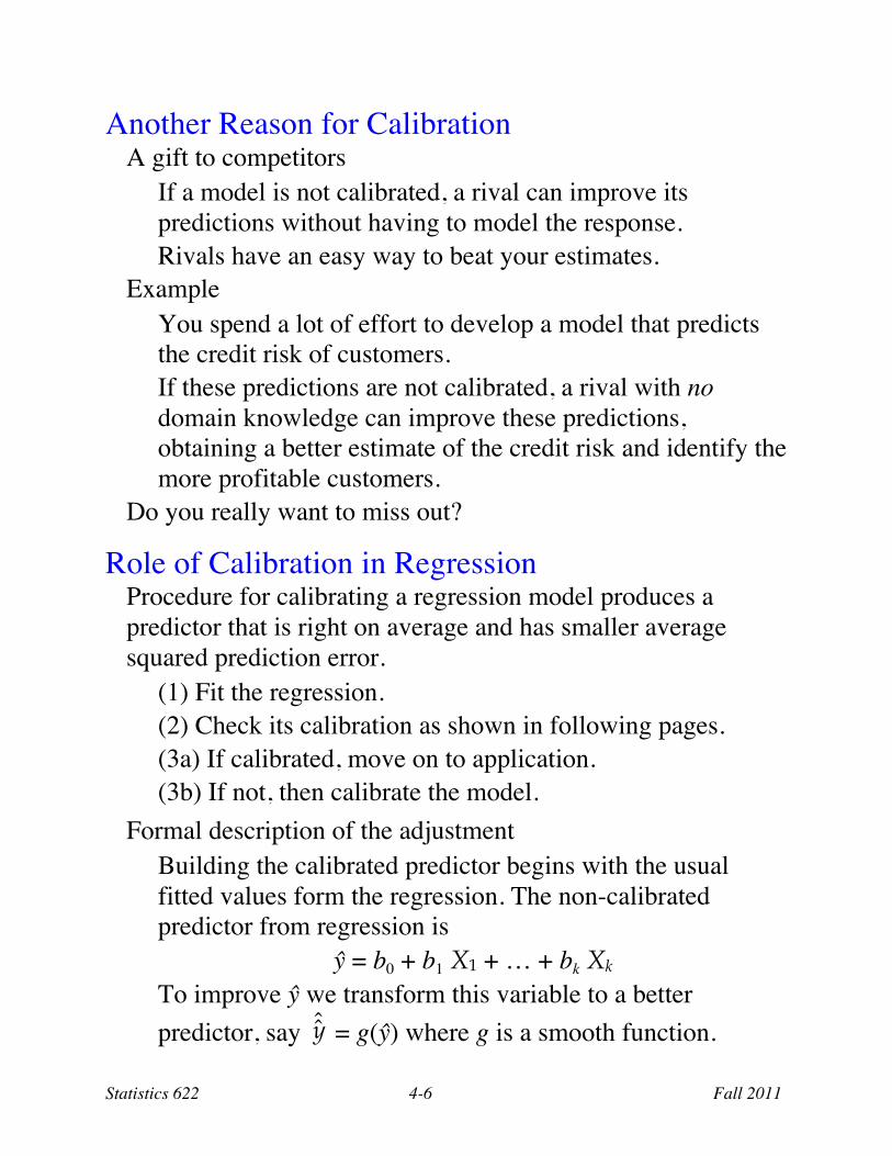
Scatterplot and linear fit
Sales = 93 + 39.8 Display Feet
The linear fit misses the average amount sold for each amount of shelf space devoted to its display. The objective is to identify a smooth curve that captures the relationship between the display feet and the amount sold at the stores.
Smoothing spline We can show the average sales for each number of display feet by adding a smoothing spline to the plot.2 A spline is a smooth curve that connects the average value of Y over a subset of values of identified by an interval of adjacent values of X.
1 This example begins in BAUR on page 12 and shows up several times in that casebook. This example illustrates the problem of resource allocation because to display more of one item requires showing less of items. The resource is the limited shelf space in stores. 2In the Fit Y by X view of the data, choose the Fit Spline option from the tools revealed by the red triangle in the upper left corner of the window. Pick the “flexible” option.
0
50
100
150
200
250
300
350
400
450Sale
s
0 1 2 3 4 5 6 7 8
Display Feet
Statistics 622 4-9 Fall 2011
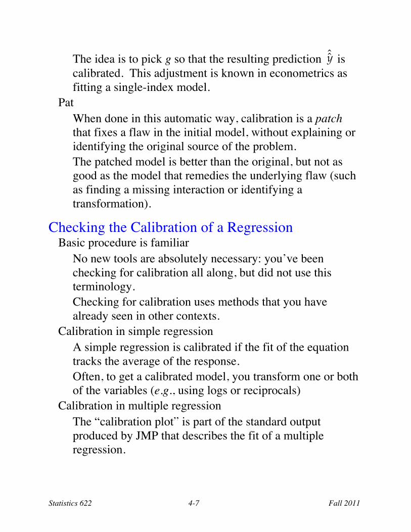
The smoothness of the spline depends on the data and can be controlled by a slider in the software. The slider controls the size of the averaged subset by controlling the range of values of X.
Example of spline In this example, a “smoothing spline” joins the mean sales for each amount sold with a smooth curve.3
With replications (several stores display the same amount; these data have several y’s for each x), the data form “columns” of dots in the plot. If the range of adjacent values of X is small enough (less than 1) then the spline joins the means of these columns.4 Without replications, the choice of a spline is less obvious and requires trial and error (i.e., guesswork).
Compare the spline to the linear fit With one foot on display, the linear fit seems too large. The mean is about $50. With two feet on display, the linear fit seems too small. The mean of sales is around $200.
3 The spline tool is easy to control. Use the slider to vary the smoothness of the curve shown in the plot. See BAUR casebook, p. 13, for further discussion of splines and these data. 4 Replications (several cases with matching values of all of the Xs) are a great asset if your data has them. Usually, they only appear in simple regression because there are too many unique combinations of predictors in multiple regression. Because the display data has replications, JMP’s “Lack of Fit” test checks for calibration. See the BAUR casebook, page 247.
0
50
100
150
200
250
300
350
400
450
Sale
s
0 1 2 3 4 5 6 7 8
Display Feet
Statistics 622 4-10 Fall 2011
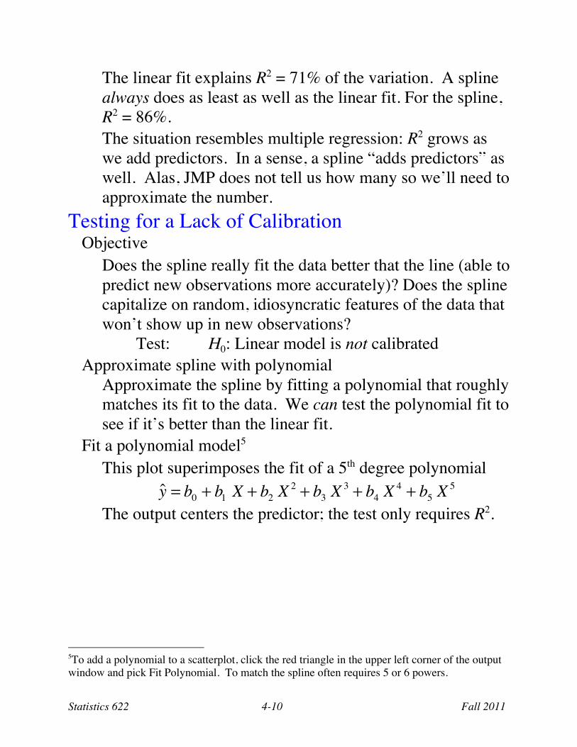
The linear fit explains R2 = 71% of the variation. A spline always does as least as well as the linear fit. For the spline, R2 = 86%. The situation resembles multiple regression: R2 grows as we add predictors. In a sense, a spline “adds predictors” as well. Alas, JMP does not tell us how many so we’ll need to approximate the number.
Testing for a Lack of Calibration Objective
Does the spline really fit the data better that the line (able to predict new observations more accurately)? Does the spline capitalize on random, idiosyncratic features of the data that won’t show up in new observations? Test: H0: Linear model is not calibrated
Approximate spline with polynomial Approximate the spline by fitting a polynomial that roughly matches its fit to the data. We can test the polynomial fit to see if it’s better than the linear fit.
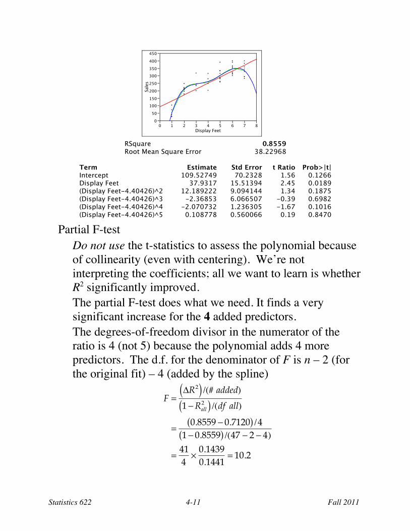
Fit a polynomial model5 This plot superimposes the fit of a 5th degree polynomial
ˆ y = b0 + b1 X + b2 X 2 + b3 X 3 + b4 X 4 + b5 X 5 The output centers the predictor; the test only requires R2.
5To add a polynomial to a scatterplot, click the red triangle in the upper left corner of the output window and pick Fit Polynomial. To match the spline often requires 5 or 6 powers.
Partial F-test Do not use the t-statistics to assess the polynomial because of collinearity (even with centering). We’re not interpreting the coefficients; all we want to learn is whether R2 significantly improved. The partial F-test does what we need. It finds a very significant increase for the 4 added predictors. The degrees-of-freedom divisor in the numerator of the ratio is 4 (not 5) because the polynomial adds 4 more predictors. The d.f. for the denominator of F is n – 2 (for the original fit) – 4 (added by the spline)
F =!R2( ) /(# added)
1 "Rall2( ) /(df all)
=0.8559 " 0.7120( ) /4
1 " 0.8559( ) /(47 " 2 " 4)
=414
#0.14390.1441
= 10.2
0
50
100
150
200
250
300
350
400
450
Sale
s
0 1 2 3 4 5 6 7 8
Display Feet
Statistics 622 4-12 Fall 2011
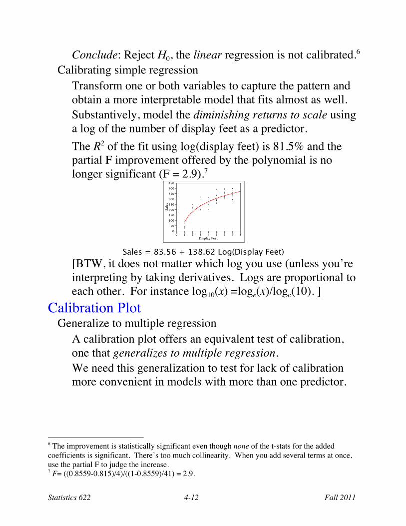
Conclude: Reject H0, the linear regression is not calibrated.6 Calibrating simple regression
Transform one or both variables to capture the pattern and obtain a more interpretable model that fits almost as well. Substantively, model the diminishing returns to scale using a log of the number of display feet as a predictor. The R2 of the fit using log(display feet) is 81.5% and the partial F improvement offered by the polynomial is no longer significant (F = 2.9).7
Sales = 83.56 + 138.62 Log(Display Feet)
[BTW, it does not matter which log you use (unless you’re interpreting by taking derivatives. Logs are proportional to each other. For instance log10(x) =loge(x)/loge(10). ]
Calibration Plot Generalize to multiple regression
A calibration plot offers an equivalent test of calibration, one that generalizes to multiple regression. We need this generalization to test for lack of calibration more convenient in models with more than one predictor.
6 The improvement is statistically significant even though none of the t-stats for the added coefficients is significant. There’s too much collinearity. When you add several terms at once, use the partial F to judge the increase. 7 F= ((0.8559-0.815)/4)/((1-0.8559)/41) = 2.9.
0
50
100
150
200
250
300
350
400
450
Sale
s
0 1 2 3 4 5 6 7 8
Display Feet
Statistics 622 4-13 Fall 2011
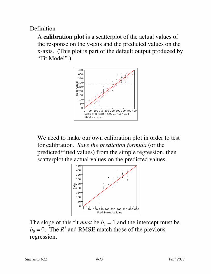
Definition A calibration plot is a scatterplot of the actual values of the response on the y-axis and the predicted values on the x-axis. (This plot is part of the default output produced by “Fit Model”.)
We need to make our own calibration plot in order to test for calibration. Save the prediction formula (or the predicted/fitted values) from the simple regression, then scatterplot the actual values on the predicted values.
The slope of this fit must be b1 = 1 and the intercept must be b0 = 0. The R2 and RMSE match those of the previous regression.
0
50
100
150
200
250
300
350
400
450
Sale
s A
ctu
al
0 50 100 150 200 250 300 350 400 450
Sales Predicted P<.0001 RSq=0.71
RMSE=51.591
0
50
100
150
200
250
300
350
400
450
Sale
s
0 50 100 150 200 250 300 350 400 450
Pred Formula Sales
Statistics 622 4-14 Fall 2011
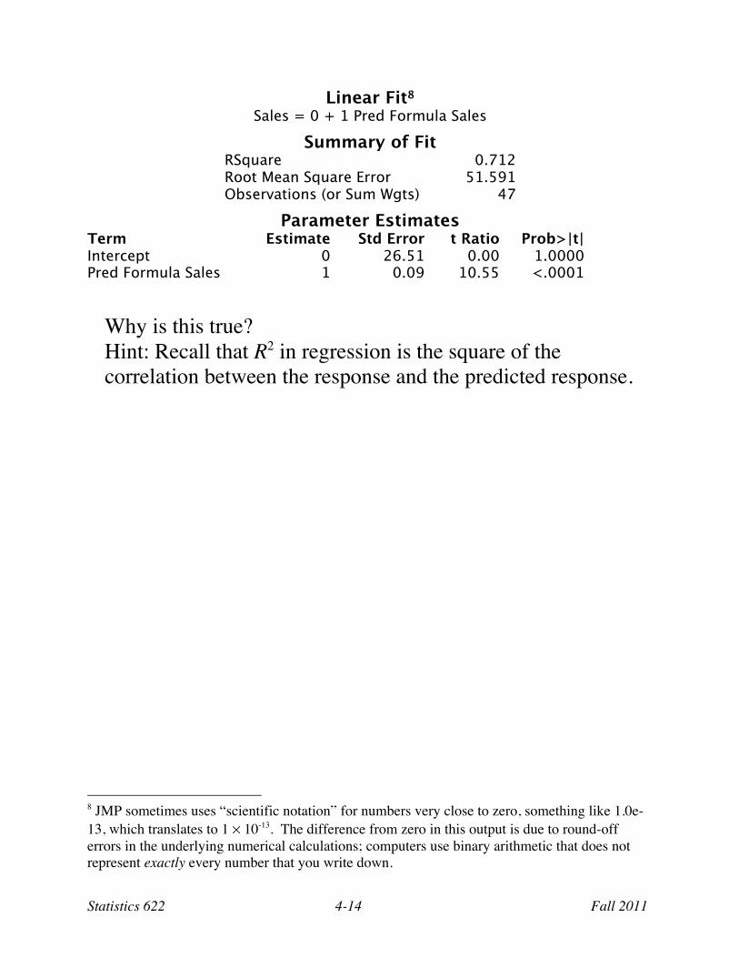
Linear Fit8 Sales = 0 + 1 Pred Formula Sales
Summary of Fit RSquare 0.712 Root Mean Square Error 51.591 Observations (or Sum Wgts) 47
Parameter Estimates Term Estimate Std Error t Ratio Prob>|t| Intercept 0 26.51 0.00 1.0000 Pred Formula Sales 1 0.09 10.55 <.0001
Why is this true? Hint: Recall that R2 in regression is the square of the correlation between the response and the predicted response.
8 JMP sometimes uses “scientific notation” for numbers very close to zero, something like 1.0e-13, which translates to 1 × 10-13. The difference from zero in this output is due to round-off errors in the underlying numerical calculations; computers use binary arithmetic that does not represent exactly every number that you write down.
Statistics 622 4-15 Fall 2011
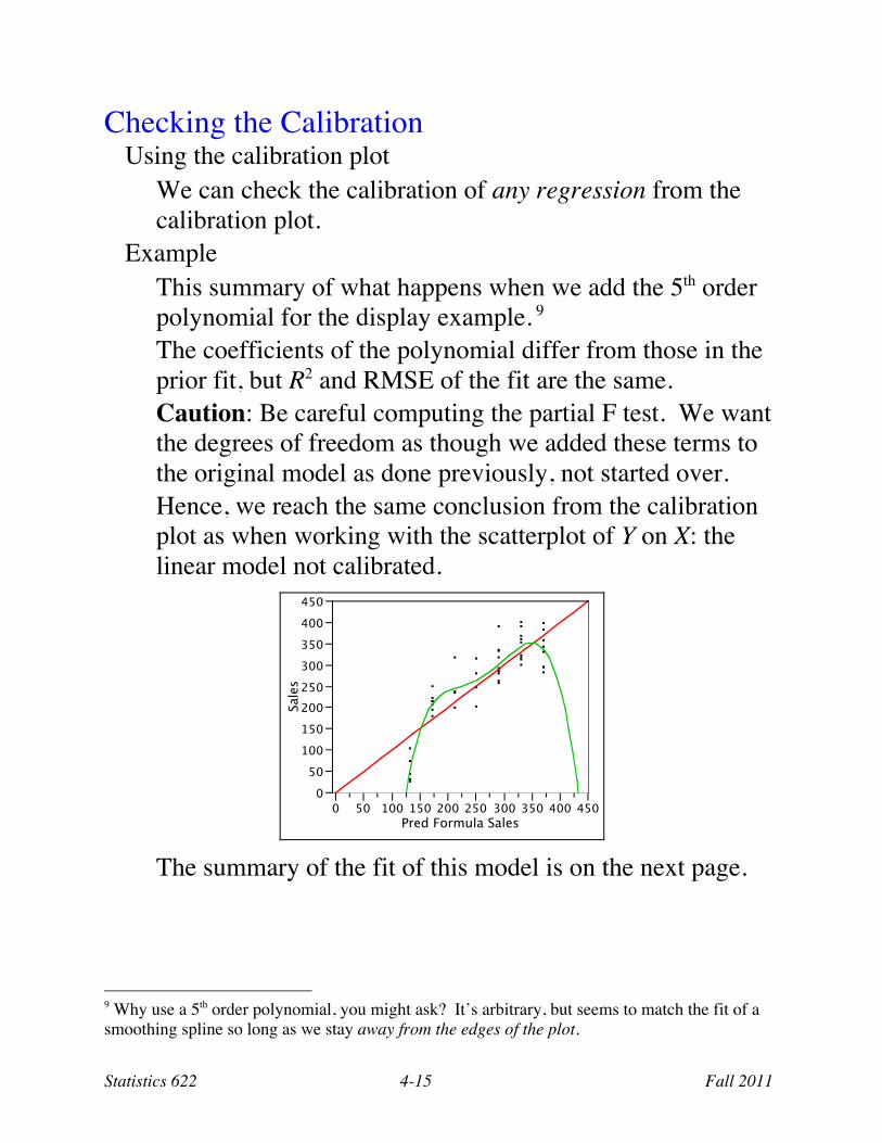
Checking the Calibration Using the calibration plot
We can check the calibration of any regression from the calibration plot.
Example This summary of what happens when we add the 5th order polynomial for the display example. 9 The coefficients of the polynomial differ from those in the prior fit, but R2 and RMSE of the fit are the same. Caution: Be careful computing the partial F test. We want the degrees of freedom as though we added these terms to the original model as done previously, not started over. Hence, we reach the same conclusion from the calibration plot as when working with the scatterplot of Y on X: the linear model not calibrated.
The summary of the fit of this model is on the next page.
9 Why use a 5th order polynomial, you might ask? It’s arbitrary, but seems to match the fit of a smoothing spline so long as we stay away from the edges of the plot.
0
50
100
150
200
250
300
350
400
450
Sale
s
0 50 100 150 200 250 300 350 400 450
Pred Formula Sales
Statistics 622 4-16 Fall 2011
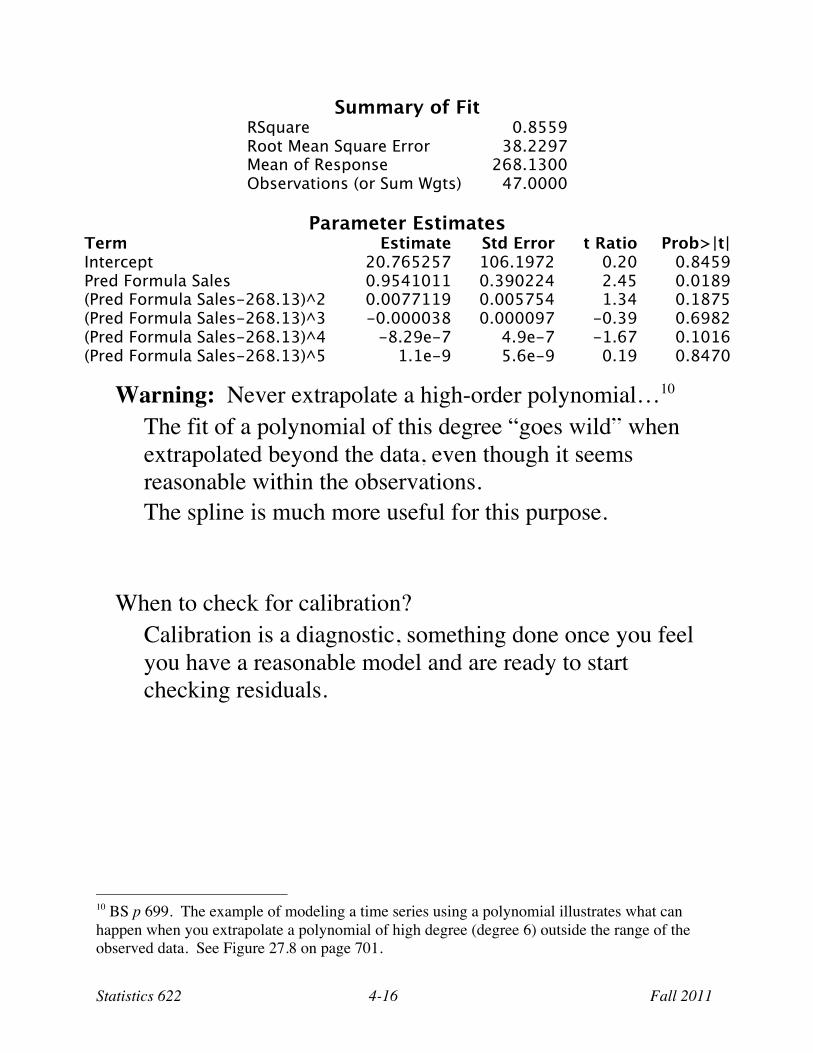
Summary of Fit RSquare 0.8559 Root Mean Square Error 38.2297 Mean of Response 268.1300 Observations (or Sum Wgts) 47.0000
Parameter Estimates
Term Estimate Std Error t Ratio Prob>|t| Intercept 20.765257 106.1972 0.20 0.8459 Pred Formula Sales 0.9541011 0.390224 2.45 0.0189 (Pred Formula Sales-268.13)^2 0.0077119 0.005754 1.34 0.1875 (Pred Formula Sales-268.13)^3 -0.000038 0.000097 -0.39 0.6982 (Pred Formula Sales-268.13)^4 -8.29e-7 4.9e-7 -1.67 0.1016 (Pred Formula Sales-268.13)^5 1.1e-9 5.6e-9 0.19 0.8470
Warning: Never extrapolate a high-order polynomial…10 The fit of a polynomial of this degree “goes wild” when extrapolated beyond the data, even though it seems reasonable within the observations. The spline is much more useful for this purpose.
When to check for calibration? Calibration is a diagnostic, something done once you feel you have a reasonable model and are ready to start checking residuals.
10 BS p 699. The example of modeling a time series using a polynomial illustrates what can happen when you extrapolate a polynomial of high degree (degree 6) outside the range of the observed data. See Figure 27.8 on page 701.
Statistics 622 4-17 Fall 2011
Checking Calibration in Multiple Regression Procedure
Use the calibration plot of y on the fitted values ŷ (a.k.a., predicted values) from the regression. (Alternatively, you can add ŷ back into the multiple regression itself.) Test the calibration by seeing whether a polynomial fit in the plot of y on ŷ significantly improves upon the linear fit that summarizes the R2 and RMSE of the regression.
Tricky part The degrees of freedom for the associated partial F test depend on the number of slopes in the original multiple regression. Thankfully, this adjustment has little effect unless you have a small sample.
Example data Model of housing prices, from the analysis of the effects of pollution on residential home prices in the 1970’s in the Boston area (introduced in Module 3). In the examples of interactions, we observed curvature in the residuals of the models. That’s a lack of calibration.
Illustrative multiple regression This regression with 5 predictors explains almost 70% of the variation in housing values. All of the predictors are statistically significant (if we accept the MRM) with tiny p-values.11 The model lacks interactions; every predictor is assumed to have a linear partial association with the prices, with a fixed slope regardless of other explanatory variables.
11 This model is part of the JMP data file; run the “Uncalibrated regression” script.
Statistics 622 4-18 Fall 2011
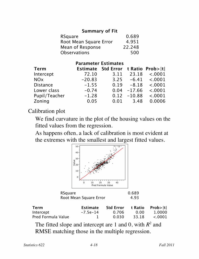
Summary of Fit
RSquare 0.689 Root Mean Square Error 4.951 Mean of Response 22.248 Observations 500
Parameter Estimates
Term Estimate Std Error t Ratio Prob>|t| Intercept 72.10 3.11 23.18 <.0001 NOx -20.83 3.25 -6.41 <.0001 Distance -1.55 0.19 -8.18 <.0001 Lower class -0.74 0.04 -17.66 <.0001 Pupil/Teacher -1.28 0.12 -10.88 <.0001 Zoning 0.05 0.01 3.48 0.0006
Calibration plot We find curvature in the plot of the housing values on the fitted values from the regression. As happens often, a lack of calibration is most evident at the extremes with the smallest and largest fitted values.
RSquare 0.689 Root Mean Square Error 4.93
Term Estimate Std Error t Ratio Prob>|t| Intercept -7.5e-14 0.706 0.00 1.0000 Pred Formula Value 1 0.030 33.18 <.0001
The fitted slope and intercept are 1 and 0, with R2 and RMSE matching those in the multiple regression.
0
10
20
30
40
50
Valu
e
0 10 20 30 40
Pred Formula Value
Statistics 622 4-19 Fall 2011
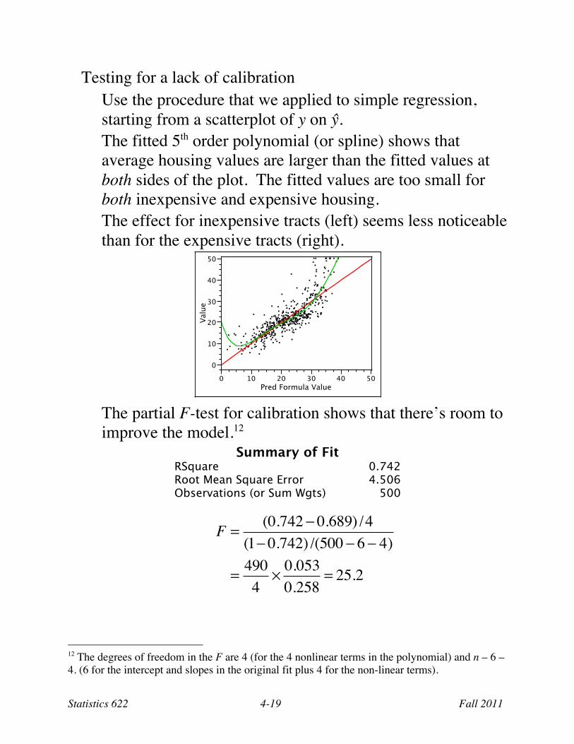
Testing for a lack of calibration Use the procedure that we applied to simple regression, starting from a scatterplot of y on ŷ. The fitted 5th order polynomial (or spline) shows that average housing values are larger than the fitted values at both sides of the plot. The fitted values are too small for both inexpensive and expensive housing. The effect for inexpensive tracts (left) seems less noticeable than for the expensive tracts (right).
The partial F-test for calibration shows that there’s room to improve the model.12
Summary of Fit RSquare 0.742 Root Mean Square Error 4.506 Observations (or Sum Wgts) 500
F = (0.742 ! 0.689) /4(1! 0.742) /(500 ! 6 ! 4)
= 4904
" 0.0530.258
= 25.2
12 The degrees of freedom in the F are 4 (for the 4 nonlinear terms in the polynomial) and n – 6 – 4. (6 for the intercept and slopes in the original fit plus 4 for the non-linear terms).
0
10
20
30
40
50
Valu
e
0 10 20 30 40 50
Pred Formula Value
Statistics 622 4-20 Fall 2011
Calibrating a Model What should be done when a model is not calibrated?
Simple regression. Ideally, find a substantively motivated transformation, such as a log, that captures the curvature. Routine “adjustments” such as those for calibration are no substitute for knowing the substance of the problem.
Multiple regression. Again, find the right transformation or a missing predictor. This can be hard to do, but some methods can find these (and indeed work for this data set and model).
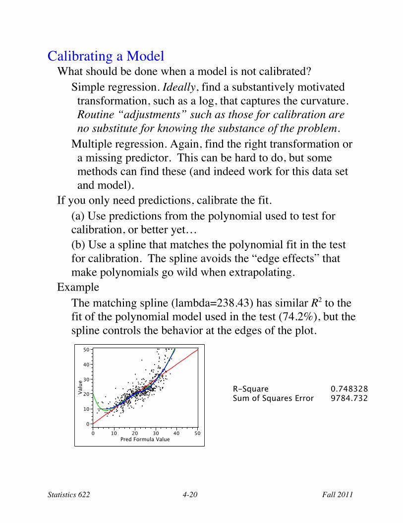
If you only need predictions, calibrate the fit. (a) Use predictions from the polynomial used to test for calibration, or better yet… (b) Use a spline that matches the polynomial fit in the test for calibration. The spline avoids the “edge effects” that make polynomials go wild when extrapolating.
Example The matching spline (lambda=238.43) has similar R2 to the fit of the polynomial model used in the test (74.2%), but the spline controls the behavior at the edges of the plot.
0
10
20
30
40
50
Valu
e
0 10 20 30 40 50
Pred Formula Value
R-Square 0.748328 Sum of Squares Error 9784.732
Statistics 622 4-21 Fall 2011
Predicting with a Smoothing Spline Use this three-step process:
1. Save predictions ŷ from the original, uncalibrated multiple regression (used to test the calibration).
2. Match a smoothing spline to the polynomial in the calibration plot (as done above).
3. Save the prediction formula from this smoothing spline as a column in the data table.
4. Insert values of ŷ from the regression into the formula for the smoothing spline to get the final prediction.
Example Predict the first row. This row is missing the response column and matches the predictors held in row #206, a case that the fitted regression under-predicts.
Predicted value from multiple regression = 39.0 Predict the response using the spline fit for cases with this predicted value. If you have saved the formula for the spline fit, this calculation happens automagically.
Predicted value from the spline = 49.5 The actual value for the matching case in row #206 is 50. The spline gives a much better estimate!
The use of a spline after a regression fixes the calibration, but avoids any attempt at explanation.
That’s a weakness. Knowing why the model under-predicts housing values at either extreme might be important.
Statistics 622 4-22 Fall 2011
Bundling the Calibration into One Regression Prediction Accuracy
The weakness of two-step calibration as done here in multiple regression is that it “hides” the nature of the original explanatory variables. We save predicted values from the multiple regression, then use these predicted values to fit a second model. Because the original explanatory variables are hidden in this second polynomial regression, that model cannot assess the accuracy of prediction – about all it can do is the back-of-the-envelope ±2 RMSE calculation.
Single model The solution – though it muddies the interpretation – is to revise the original multiple regression rather than fit a second, separate polynomial regression. Simply add the powers of the predicted values y2, y3, y4, y5(note, omitting the 1st power) back into the original regression.13 As a bonus, since all of the effects are together in one model, we can (a) use familiar regression summaries, such as the profile plots or leverage plots. (b) use tests provided by the multiple regression, such as the custom test for the added terms.
13 JMP makes this easy. Recall the fitted multiple regression, set the Degree item to 5, select the predicted value column, and finally use the Macro > Polynomial to Degree button to add powers of the predicted values. Just remember to remove the 1st power. Easier done than said.
Statistics 622 4-23 Fall 2011
Collinearity The addition of these powers adds quite a bit of collinearity that will obscure the effects of the original explanatory variables, so you will need to return to the original equation to interpret them. Be sure centering is turned on for a bit less collinearity. It would be better to add so-called “orthogonal polynomials” to the regression, but that requires more “manual” calculations, so we’ll not go there.
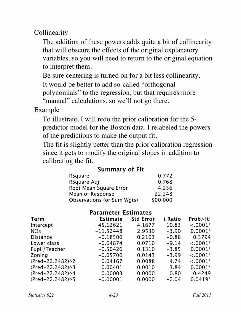
Example To illustrate, I will redo the prior calibration for the 5-predictor model for the Boston data. I relabeled the powers of the predictions to make the output fit. The fit is slightly better than the prior calibration regression since it gets to modify the original slopes in addition to calibrating the fit.
Summary of Fit RSquare 0.772 RSquare Adj 0.768 Root Mean Square Error 4.256 Mean of Response 22.248 Observations (or Sum Wgts) 500.000
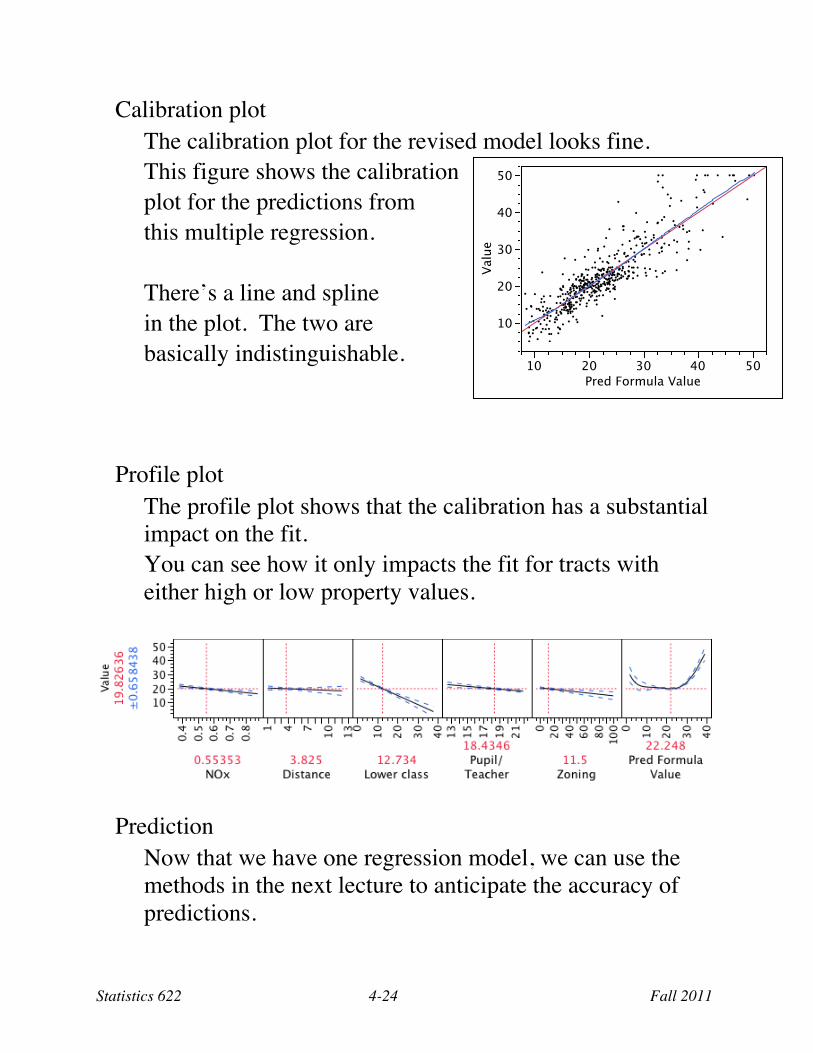
Calibration plot The calibration plot for the revised model looks fine. This figure shows the calibration plot for the predictions from this multiple regression. There’s a line and spline in the plot. The two are basically indistinguishable.
Profile plot
The profile plot shows that the calibration has a substantial impact on the fit. You can see how it only impacts the fit for tracts with either high or low property values.
Prediction Now that we have one regression model, we can use the methods in the next lecture to anticipate the accuracy of predictions.
10
20
30
40
50
Val
ue
10 20 30 40 50Pred Formula Value
Statistics 622 4-25 Fall 2011
Other Forms of Calibration When a model predicts the response right, on average, we might ought to say that the model is calibrated to first order. Higher-order calibration matters as well:
(a) Second-order calibrated: the variation around every prediction is a known or correctly estimated (including capturing changes in error variation). (b) Strongly calibrated: the distribution of the prediction errors is known or correctly estimated (such as with a normal distribution).
We typically check these as part of the usual regression diagnostics, after we get the right equation for the mean value. That’s the message here as well:
Get the predicted value right on average, then worry about the other attributes of your prediction.
Discussion Some points to keep in mind…
• The reason to calibrate a model is so that the predictions are correct, on average. Economic decision-making requires calibrated predictions. As a by-product, the model also has smaller RMSE. • We fit the polynomial to test for calibration only because JMP’s spline tool does not tell us the information needed to use the partial F test (i.e., the number of added variables) • Splines are subject to personal impressions. Methods are available (not in JMP) that provide a more objective measure of how much to smooth the fit.