Large Bets and Stock Market Crashes Albert S. Kyle and Anna A. Obizhaeva * First Draft: March 5, 2012 This Draft: July 3, 2013 For five stock market crashes, we compare price declines with pre- dictions from market microstructure invariance. Predicted price de- clines half as large as the 1987 crash and almost equal to the 2008 sales of Soci´ et´ e G´ en´ erale suggest that useful early warning systems are feasible. Larger-than-predicted temporary price declines during two flash crashes suggest rapid selling exacerbates transitory price impact. Smaller-than-predicted price declines for the 1929 crash sug- gest slower selling stabilized prices and less integration made markets more resilient. Quantities sold in the three largest crashes suggest fatter tails or larger variance than the log-normal distribution esti- mated from portfolio transitions data. JEL: G01, G28, N22 Keywords: finance, market microstructure, invariance, crashes, liq- uidity, price impact, market depth, systemic risk * Kyle: Robert H. Smith School of Business, University of Maryland, College Park, MD 20742, [email protected]. Obizhaeva: Robert H. Smith School of Business, University of Maryland, College Park, MD 20742, [email protected]. 1
Transcript
Large Bets and Stock Market Crashes
Albert S. Kyle and Anna A. Obizhaeva∗
First Draft: March 5, 2012
This Draft: July 3, 2013
For five stock market crashes, we compare price declines with pre-dictions from market microstructure invariance. Predicted price de-clines half as large as the 1987 crash and almost equal to the 2008sales of Societe Generale suggest that useful early warning systemsare feasible. Larger-than-predicted temporary price declines duringtwo flash crashes suggest rapid selling exacerbates transitory priceimpact. Smaller-than-predicted price declines for the 1929 crash sug-gest slower selling stabilized prices and less integration made marketsmore resilient. Quantities sold in the three largest crashes suggestfatter tails or larger variance than the log-normal distribution esti-mated from portfolio transitions data.
∗ Kyle: Robert H. Smith School of Business, University of Maryland, College Park, MD20742, [email protected]. Obizhaeva: Robert H. Smith School of Business, University ofMaryland, College Park, MD 20742, [email protected].
1
1
After stock market crashes, rattled market participants, frustrated policymakers,and puzzled economists are typically unable to explain what happened. In theaftermath, studies have documented unusually heavy selling pressure during theseepisodes. According to conventional wisdom, however, stock markets have suchgreat liquidity that the dollar magnitudes of large sales are far too small to explainobserved declines in prices.We question the conventional wisdom from the perspective of market microstruc-
ture invariance, a conceptual framework developed by Kyle and Obizhaeva (2013).Combined with a linear price impact model, invariance can explain why order flowimbalances, expressed as a fraction of average daily volume, result in greater priceimpact in large markets than in small markets. As a result, when market impactestimates based on applying invariance to individual stocks are extrapolated to theentire stock market, price impact estimates become large enough to explain stockmarket crashes.We study five crash events, chosen because data on the magnitude of selling
pressure became publicly available in the aftermath:
• After the stock market crash of October 1929, the report by the Senate Com-mittee on Banking and Currency (1934) (the “Pecora Report”) attributed thedramatic plunge in broker loans to forced margin selling during the crash.
• After the October 1987 stock market crash, the U.S. Presidential Task Forceon Market Mechanisms (1988) (the “Brady Report”) documented quanti-ties of stock index futures contracts and baskets of stocks sold by portfolioinsurers during the crash.
• After the futures market dropped by 20% at the open of trading three daysafter the 1987 crash, the Commodity Futures Trading Commission (1988)documented large sell orders executed at the open of trading; the press iden-tified the seller as George Soros.
• After the Fed cut interest rates by 75 basis points in response to a worldwidestock market plunge on January 21, 2008, Societe Generale revealed that ithad quietly been liquidating billions of Euros in stock index future positionsaccumulated by rogue trader Jerome Kerviel.
• After the flash crash of May 6, 2010, the Staffs of the CFTC and SEC(2010b,a) cited as a trigger large sales of futures contracts by one entity,identified in the press as Waddell & Reed.
We call these large sales “bets.” A bet is an “intended order” or “meta-order”whose size is known in advance of trading. Large bets can result either fromtrading by one large entity or from correlated trades of multiple entities based onthe same underlying motivation. In a speculative market, price fluctuations occurwhen some investors place bets which move prices, while other traders attempt toprofit by intermediating among the bets being placed. Execution of very large betscan lead to significant market dislocations.
2
While accurate estimates of the size of potential selling pressure were publishedand widely discussed months before the crashes of 1929 and 1987, market partic-ipants had different opinions concerning whether the selling pressure would havea significant effect on prices. Before the three crash events associated with theSoros trades, the Societe Generale trades, and the flash crash trades, the sellersknew precisely the quantities they intended to sell, but they either estimated inac-curately or were willing to incur large transaction costs. For all five crash events,policymakers or stock market participants had in hand the information market mi-crostructure invariance requires to quantify the price impact and thus the systemicrisks resulting from sudden liquidations of large stock market exposures.Market microstructure invariance is based on the intuition that “business time”
passes more quickly in active markets than in inactive markets. When appropriateadjustment is made for the rate at which business time passes, market propertiesrelated to the dollar rate at which mark-to-market gains and losses are generateddo not vary across markets. Since business time operates at a much faster pacein equity markets as a whole than in less active markets for individual stocks,one calendar day in equity index markets is equivalent to many calendar days inmarkets for individual stocks. Sales of a given percentage of daily volume in equityindices are effectively equivalent to the same percentage of volume executed overmany consecutive days in individual stocks and therefore lead to much greaterprice impacts than trades of a similar magnitude in individual stocks. In this way,the invariance principle implies far greater price impacts for large sales of equityindices than conventional wisdom suggests.Two features of microstructure invariance make practical predictions possible.
First, the invariance principle generates precise formulas for market impact, theimplementation of which requires only a small number of parameters to be es-timated. These parameter values are the same for active markets and inactivemarkets, liquidations of large positions and liquidations of small positions. Wetherefore extrapolate to the entire market the parameters Kyle and Obizhaeva(2013) obtain from a database of more than 400,000 portfolio transition trades inindividual stocks. Second, given parameter estimates, price impact estimates arefunctions of expected dollar volume, expected returns volatility, and the dollar sizeof amounts traded. It is not necessary to have additional information about othermarket characteristics, such as dealer market structure, information asymmetries,the motivation of traders, or order shredding algorithms.Our estimates of price impact are much greater than implied by conventional
wisdom. We define “conventional wisdom” as the idea that the demand for indi-vidual stocks or for the entire stock market is “elastic” in the sense that sellingone percent of market capitalization has a price impact of less than one percent.This definition is similar to the related idea that the price impact of selling 5-10percent of average daily volume is modest, either for an individual stock or stockindex futures.Table 1 summarizes our results for each of the five crash events. Using volume
3
and volatility estimated from daily data over the month before the crash event, thetable shows the estimated size of the dollar amounts liquidated (percent of dailyvolume and GDP), actual price declines (percent), and price declines predicted byinvariance and conventional wisdom (percent).
Table 1—Summary of Five Crash Events: Actual and Predicted Price Declines.
Actual Predicted Predicted %ADV %GDPInvariance Conventional
Table 1 shows that three of the crash events involve much larger selling pressurethan the other two. The 1929 crash, the 1987 crash, and the Societe Generaletrades of 2008 all involve sales of more than 25% of average daily volume or morethan 0.25% of GDP. By contrast, the sales by Soros in 1987 and the flash crashof 2010 both involve sales of only 2.29% and 1.49% of average daily volume theprevious month.Overall, the price declines predicted by invariance are much closer in magnitude
to actual price declines than predictions based on conventional wisdom, but thereis substantial variation across crash events. Compared with actual price declines,the declines predicted by invariance are about twice as large for the 1929 crash,about the same for the Societe Generale liquidation, about half as large for the1987 crash, and much smaller for the 1987 Soros trades and the 2010 flash crashtrades. By contrast, the price impact estimates based on conventional wisdom areminuscule in comparison to actual price changes.The differences between actual and predicted price declines suggest explanations
for how price impact may be influenced circumstances surrounding execution oflarge bets.For the 1929 stock market crash, the actual price decline of 25% was much smaller
than the predicted decline of 46.43%. This may be explained by efforts financialmarkets made to spread the impact of margin selling out over several weeks ratherthan several days, by greater resiliency of markets resulting from less financialintegration, or by potential buyers keeping capital on the sidelines to profit fromprice declines widely expected to occur if margin purchases were liquidated.For the 1987 stock market crash, the actual decline of 32% was approximately
double the predicted decline of 16.77%. Perhaps price declines were exacerbatedby breakdowns in the market mechanism documented in the Brady Report. Forthe 2008 Societe Generale trades, the actual decline of 9.44% was similar to the
4
predicted price decline of broad European indices by 10.79%. From a theoreticalperspective, it is puzzling that the unanticipated trades by Societe Generale ap-pear to have had smaller impact, relative to the invariants benchmark, than theanticipated trades by the portfolio insurers.The remaining two crashes are both “flash-crash” events in which the trades
were executed in minutes, not hours. The actual plunges in prices associated withSoros’s 1987 trades and the 2010 flash crash, 22% and 5.12% respectively, aremuch larger than the declines predicted by invariance, 6.27% and 0.61% respec-tively. Both flash crashes were followed minutes later by rapid rebounds in prices.We hypothesize that the rapid speed, large size, and immediate reversals of thelarge price declines resulted from the unusually rapid rate at which these tradeswere executed. This hypothesis is consistent with the theoretical model of Kyle,Obizhaeva and Wang (2013).Since invariance generates predictions about the frequency and the size distribu-
tion of bets, it also has implications for the frequency and magnitude of crashes.Under the identifying assumption that portfolio transition orders have the samesize distribution as bets, Kyle and Obizhaeva (2013) find that the distributionof unsigned bet sizes closely resembles a log-normal with variance of 2.53; itssignificant kurtosis suggests occasional crashes. The two flash-crashes representapproximately 4.5-standard-deviation bet events, which are expected to occur sev-eral times per year. We do not include in this study flash crash events in 1961and 1989, as well as others, due to lack of data on selling pressure. The threelargest crashes are approximately 6-standard-deviation bet events. Based on thelog-normal distribution, they are expected to occur less frequently, only once inhundreds or thousands of years. Obviously, the actual frequency of crashes is farhigher than implied by fitting a log-normal distribution to portfolio transition data.Either the tails of the distribution are fatter than a log-normal—consistent with apower law—or the variance is larger than estimated from portfolio transition data.In what follows are sections discussing conventional wisdom and the animal spir-
its hypothesis, market microstructure invariance, particulars of each of the fivecrash events, the frequency of crashes, and lessons learned.
I. Conventional Wisdom, Animal Spirits, andBanking Crises
The debate about what causes market crashes started before the 1929 crash.Since then, economists and market participants have been divided into two campswhich differ in their views concerning whether crashes result from rational or irra-tional behavior. We call explanations based on rationality “conventional wisdom”and explanations based on irrationality “animal spirits.” After more than 80 years,the debate has made little progress. Neither of these two camps has offered a com-pelling explanation for crashes.
5
Conventional Wisdom.
Conventional wisdom holds that large price changes result from arrival of newfundamental information into the market, not from the price pressure resultingfrom buying and selling. In the 1960s and 1970s, this conventional wisdom becameassociated with the capital asset pricing model and efficient markets hypothesis.Conventional wisdom based on the capital asset pricing model implies that thedemand for market indices is elastic and that demand for individual stocks is evenmore so; the quantities observed changing hands in the market are too small toexplain dramatic plunges in market prices. Empirical studies based on the analysisof secondary distributions (e.g., Scholes (1972)), index inclusions and deletions(e.g., Harris and Gurel (1986) and Wurgler and Zhuravskaya (2002)), and otherevents usually find that selling one percent of shares outstanding has a price impactof less than one percent. By extrapolating this conventional wisdom to equityindices, researchers and regulators have concluded that stock market crashes donot result from selling pressure.Views consistent with the conventional wisdom based on the capital asset pricing
model are shared by many prominent economists.Miller (1991), for example, states the following about the 1987 crash: “Putting
a major share of the blame on portfolio insurance for creating and overinflatinga liquidity bubble in 1987 is fashionable, but not easy to square with all relevantfacts. . . . No study of price-quantity responses of stock prices to date supports thenotion that so large a price decrease (about 30%) would be required to absorb somodest (1-2%) a net addition to the demand for shares.”As the academics most associated with portfolio insurance, Leland and Rubin-
stein (1988) echo this argument: “To place systematic portfolio insurance in per-spective, on October 19, portfolio insurance sales represented only 0.2% of totalU.S. stock market capitalization. Could sales of 1 in every 500 shares lead to adecline of 20% in the market? This would imply a demand elasticity of 0.01—virtually zero—for a market often claimed to be one of the most liquid in theworld.”Brennan and Schwartz (1989) note that portfolio insurance would have a minimal
effect on prices, because most portfolio-consumption models imply elasticities ofdemand for stock more than 100 times the elasticities necessary to explain the 1987crash.Conventional wisdom based on the efficient markets hypothesis can be interpreted
as implying that, since many investors compete for information, it would be highlyunusual for investors to have private information of sufficient value so that theinformation content of their trades would move the entire stock market significantly.Restricting trading to be a given percent of daily trading volume, for example fiveor ten percent, will have price impact close to zero. Since turnover is usuallyabout 100% per year, the intuition about the costs of execution a small percentageof daily trading volume is closely related to the intuition about execution of a tinypercentage of market capitalization.
6
Based on this intuition, the Brady Report, comparing the 1929 and 1987 crashes,comes to the following conclusion about the 1929 crash: “To account for the con-temporaneous 28% decline in price, this implies a price elasticity of 0.9 with respectto trading volume which seems unreasonably high. As a percentage of total sharesoutstanding, margin-related selling would have been much smaller. Viewed as ashift in the overall demand for stocks, margin-related selling could have accountedrealistically for no more than 8% of the value of outstanding stock. On this basis,the implied elasticity of demand is 0.3 which is beyond the bound of reasonableestimates.”Many observers of the 1987 stock market crash, including Miller (1988, p. 477)
and Roll (1988), looked therefore to explanations other than the price pressure ofthe large quantities traded to explain the large changes in prices.We disagree with the conventional wisdom. For all five crash events, it is difficult
to find new fundamental information shocks to which market prices would havereacted with the magnitude of price declines actually observed. We are left withthe puzzling fact that large sales—even when known to have no information con-tent, such as the margin sales of 1929 or the portfolio insurance sales in 1987—doappear to have large effects of prices. Our examination of five historical episodesthrough the lens of invariance shows that actual price changes are indeed similarin magnitude to those predicted by extrapolating estimates from data on portfoliotransitions for individual stocks in normal market conditions to unusually largebets on market indices.
Animal Spirits Hypothesis.
Animal spirits holds that price fluctuations occur as a result of random changesin psychology, which may not be based on economically relevant information orrationality. The term “animal spirits” is associated with Keynes (1936), who saysthat financial decisions can be taken only as the result of “animal spirits—a spon-taneous urge to action rather than inaction, and not as the outcome of a weightedaverage of quantitative benefits multiplied by quantitative probabilities.” Akerlofand Shiller (2009) echo Keynes: “To understand how economies work and howwe can manage them and prosper, we must pay attention to the thought patternsthat animate people’s ideas and feelings, their animal spirits.” According to ani-mal spirits theory, market crashes occur when decisions are driven by changes inmind set based on emotions and social psychology instead of rational calculations.Promptly after the 1987 crash, for example, Shiller (1987) surveyed traders andfound that “most investors interpreted the crash as due to the psychology of otherinvestors.”We disagree with animal spirits theory. Although the timing of crash events
may be unpredictable, market participants had mundane pre-crash explanationsfor why both the 1929 and 1987 crashes might occur. These explanations wereremarkably accurate and did not involve animal spirits. In the months prior tothe 1929 stock market crash, brokers were raising margin requirements to protect
7
themselves from a widely discussed collapse in prices which might be induced byrapid unwinding of stock investments financed with margin loans. In the monthsprior to the 1987 stock market crash, the SEC—responding to worries that port-folio insurance made the market fragile—published a study describing a cascadescenario induced by portfolio insurance sales. On the day the 1987 crash occurred,academics were holding a conference on a potential “market meltdown” induced byportfolio insurance sales. It would be implausible to argue that a sudden change inanimal spirits occurred coincidentally on the same day Societe Generale liquidatedKerviel’s rogue trades. While the sales of George Soros in 1987 may reflect theanimal spirits of this one person, the rapid recovery of prices after both flash crashevents do not suggest market-wide irrationality or psychological contagion. Theysuggest the opposite.
Stock Market Crashes and Banking Crises.
The five stock market crashes differ from the long-lasting financial crises cat-alogued by Reinhart and Rogoff (2009), who examine sovereign defaults, bank-ing crises associated with collapse of the banking system, exchange rate crisesassociated with currency collapse, and bouts of high inflation. Reinhart and Ro-goff (2009) document that it usually takes many years and significant changesin macroeconomic policies and market regulations for the affected economies torecover from these fundamental problems associated with insolvency of financialinstitutions underlying the economy.In contrast, stock market crashes or panics triggered by large bets are likely to be
short-lived if followed by appropriate government policy. For example, the FederalReserve System implemented an appropriately loose monetary policy immediatelyafter the 1929 crash, which calmed down the market by the end of 1929. The greatdepression of the 1930s resulted from a subsequent shift towards a deflationarypolicy, not the 1929 crash. After the liquidation of Jerome Kerviel’s rogue trades in2008, an immediate 75-basis point interest rate cut by the Fed may have preventedthis event from immediately spiraling into a deeper financial crisis, but it did notprevent the collapse of Bear Stearns a few weeks later. It was the bursting of thereal estate credit bubble, not the unwinding of Jerome Kerviel’s fraud, that led tothe deep and long-lasting recession which unfolded in 2008-2009.
II. Market Microstructure Invariance
Market microstructure invariance is based on the simple intuition that stockmarket trading is a game played by professional traders, the “rules” of the tradinggame are the same across stocks and across time, but the speed with which thegame is played varies across stocks based on levels of trading activity. The tradinggame is played faster if securities have higher levels of trading volume and volatility.Trading in speculative markets transfers risks among traders. We refer to these
risk transfers as “bets.” Bets are sometimes called “meta-orders.” Asset specific
8
“business time” passes at a rate proportional to the rate at which bets arrive.Microstructure invariance conjectures that the distribution of standard deviationsof gains and losses on bets is the same across markets, when measured in units ofbusiness time. In this sense, the rate at which speculative markets transfer riskis invariant, when adjusted for the speed with which trading occurs. Invariancealso conjectures that the expected dollar transactions cost of executing a bet isconstant across markets, when the size of the bet is measured as the dollar risktransferred per unit of business time. As discussed by Kyle and Obizhaeva (2013),these scaling principles place strong restrictions on both the size distribution ofbets and their market impact as a function of observable dollar trading volumeand volatility.We examine the implications of a log-linear version of the linear price impact
model from Kyle and Obizhaeva (2013). The expected percentage price impactfrom buying or selling X shares of a stock with a current stock price P dollars,expected trading volume V shares per calendar day, and expected daily percentagestandard deviation of returns σ is given by
(1) ln
(1 +
∆P (X)
P
)=
λ
104·(
P · V40 · 106
)1/3
·( σ
0.02
)4/3· X
(0.01)V.
Invariance imposes the restriction that the price impact of a bet of fraction X/Vof expected daily volume is proportional to the product of the cube root of dollarvolume P ·V and the 4/3 power of volatility σ. Invariance implies that the propor-tionality factor is the same for all markets, large and small. In equation (1), thisproportionality factor is expressed in terms of a price impact parameter λ, whichis scaled so that it measures in basis points the market impact of trading X = 1%of expected daily volume V of a hypothetical “benchmark stock” with stock priceof P = $40 per share, expected volume V = 1 million shares per day, and volatilityσ = 2% per day.We infer a value of λ from price impact costs that Kyle and Obizhaeva (2013)
estimate by applying the concept of implementation shortfall to a dataset of morethan 400,000 portfolio transition orders. A portfolio transition occurs when assetsunder the management of one institutional asset manager are transferred to anotheranother. Trades converting the legacy portfolio into the new portfolio are typicallyhandled by a professional third-party transition manager. Implementation short-fall, as discussed by Perold (1988), is the difference between actual execution pricesand prices based on transactions-cost-free “paper trading” at prices observed in themarket just before the order is placed. Portfolio transition trades are ideal for us-ing implementation shortfall to estimate transactions costs because the exogeneityof the order sizes eliminates selection bias.Kyle and Obizhaeva (2013) estimate an average impact cost parameter κI = 2.50
basis points (standard error 0.19 basis points). Large orders are broken into piecesand executed at prices which tend to increase due to movement along an upwardsloping demand schedule, which we assume to be approximately linear. Thus, we
9
assume that total price impact is twice the average impact cost, i.e., λ = 2 · κI =5.00 basis points. Although invariance also has implications for bid-ask spreadcosts, these costs are negligible for large bets; hence, we ignore them.The connection between short-term impact and long-term impact is not straight-
forward. Equation (1) describes short-term price impact. The long term impact ofa bet depends on the information content of the bet itself. Mean-reversion occurredwithin minutes after both flash crashes, within a few day’s after the liquidation ofKerviel’s rogue positions in 2008, and over weeks and months after market crashesof 1929 and 1987.Invariance is consistent with both linear and non-linear specifications for market
impact. Kyle and Obizhaeva (2013) calibrate both linear and square root priceimpact functions. From a theoretical perspective, the linear model is attractivebecause it is broadly consistent with the market microstructure literature, e.g.,the linear impact model of Kyle (1985). From an empirical perspective, Kyleand Obizhaeva (2013) find that the square root specification explains price impactbetter than the linear model, a finding consistent with the empirical econophysicsliterature (Bouchaud, Farmer and Lillo, 2009). Kyle and Obizhaeva (2013) alsofind that the linear model explains the price impact of the largest one percent ofbets in the most active stocks slightly better than the square root model.Due to its concavity, the square root model predicts much smaller price declines
during crash events than the linear model. Invariance alone does not explain crashevents; instead, crash events are explained by applying invariance to a linear model.To make this point, “invariance” assumes a linear impact function in the rest ofthis paper.We choose to consider log-linear market impact rather than simple linear market
impact as in Kyle and Obizhaeva (2013), because our analysis deals with verylarge orders, sometimes equal in magnitude to trading volume of several tradingdays. In contrast, Kyle and Obizhaeva (2013) consider relatively smaller portfoliotransition orders with an average size of about 4.20% of daily volume and mediansize of 0.57% of daily volume. For these orders, the distinction between continuouscompounding and simple compounding is immaterial.Equation (1) describes market impact during both normal times and times of
crash or panic, for individual stocks and market indices. The five crashes occurredin markets with high trading volume, typically during times of significant volatil-ity. Because of high trading volume and volatility, the market impact implied byequation (1) is greater than the impact obtained from conventional wisdom.The difference between the linear price impact function implied by invariance
and a linear price impact function consistent with conventional wisdom can beillustrated using the model of Kyle (1985). Equation (1) can be thought of asan implementation of the formula λ = σV /σU from Kyle (1985) in units of busi-ness time. The conventional wisdom about market impact arises from a naiveimplementation of the the same formula in units of calendar time. Under the as-sumptions that the standard deviation of fundamentals σV is proportional to price
10
volatility σ · P and the standard deviation of order imbalances σU is proportionalto dollar volume V , price impact can be written
(2) ln
(1 +
∆P (X)
P
)=
λ
104·( σ
0.02
)· X
(0.01)V.
This equation is consistent with our definition of conventional wisdom if neitherturnover rates nor volatility vary much across stocks: Price impact of a fixedfraction of volume is similar across markets regardless of their dollar volume.A comparison of impact implied by invariance in equation (1) with the impact
implied by conventional wisdom in equation (2) reveals that the price impact ofa bet differs by a factor proportional to (P · V · σ)1/3. Thus, when dollar volumeP ·V is increased by a factor of 1, 000—approximately consistent with dollar volumedifferences between a benchmark stock and stock index futures—invariance impliesthat market impact changes by a factor (1000)1/3 = 10 times greater than impliedby conventional wisdom. Furthermore, according to conventional wisdom, doublingvolatility doubles the market impact of trading a given percentage of expecteddaily volume. According to invariance, the price impact increases by a factor of24/3 ≈ 2.52. When these effects of volume and volatility are taken into account, weconclude that the observed market dislocations may have resulted from the sellingpressure observed in active and volatile markets.Market participants often execute large orders in individual stocks by restricting
quantities traded to be not more than five or ten percent of average daily volumeover a period of several days. Conventional wisdom implies that the same strategywill also be reasonable in more active markets such as markets for stock indexfutures. In contrast, invariance predicts that this heuristic strategy may incurmuch larger transaction costs when implemented in active markets.Kyle and Obizhaeva (2013) define “trading activity” W as the product of dol-
lar volume and volatility, W := V · P · σ. Conceptually, trading activity is thestandard deviation of one calendar day’s dollar mark-to-market gains or losses ontrading volume expected to be executed during a calendar day. For the benchmarkstock, trading activity is defined s W ∗ := 40 · 106 · 0.02 = 800, 000. Let Q denotethe number of shares in a bet, positive for buys and negative for sells. Invarianceimplies that the distribution of bet size as a fraction of volume is such that dis-tribution |Q/V | · (W/W ∗)−2/3 is the same for all stocks. Empirically, Kyle andObizhaeva (2013) find that distribution of portfolio transition orders is approx-imately symmetric about zero, with unsigned order size close to the log-normalln(|Q/V |) ∼ N(−5.71− 2/3 · ln(W/W ∗), 2.53).Figure 1 compares the five crash events with large portfolio transition orders.
The horizontal axis is the log of scaled trading activity ln(W/W ∗). The verticalaxis is the log of order size as a fraction of expected daily volume. The horizontalline |Q/V | = 5% represents an order equal to 5% of daily volume. The lowest(red) diagonal line, which has a slope of −2/3 represents a median bet |Q/V | asimplied by invariance; it intersects the vertical axis at −5.71, for the benchmark
11
-12
-10
-8
-6
-4
-2
0
2
4
-12 -7 -2 3 8
median
order size
(invariance)
Q/V=5%
ln(Q/V)
ln(W/W*)
1929 crash
1987 crash
1987 Soros
2008 SocGen
Flash Crash
std1
std2
std3
std4
std5
std6
std0
Figure 1. Largest Portfolio Transition Orders and Market Crashes.
Figure shows the largest portfolio transition orders for each month from January 2001 to Decem-ber 2005 and for each of ten volume groups (blue points) as well as the bets during five marketcrashes (red points). Volume groups are based on thresholds corresponding to 30th, 50th, 60th,70th, 75th, 80th, 85th, 90th, and 95th percentiles of the dollar volume for common NYSE-listedstocks. The vertical axis is | ln(Q/V )|. The horizontal axis is ln(W/W ∗), whereW ∗ = 40·106 ·0.02and W = V · P · σ. The median order is −5.71 − 2/3 · ln(W/W ∗) (red line). The x-standarddeviation events are −5.71− 2/3 · ln(W/W ∗) + x ·
√2.53 (green lines).
stock, implying a median bet in the benchmark stock equal to exp(−5.71) ≈ 0.33%of daily volume. The six parallel diagonal lines above represent orders whose log-size is one through six standard deviations above the median size, respectively, asimplied by invariance; the vertical distance between each line is the log-standarddeviation of 2.531/2 ≈ 1.60. Each log standard deviation represents a factor ofexp(2.531/2) ≈ 4.90 in unsigned order sizes.For each of the 60 months from January 2001 through December 2005, each of
the 400,000+ portfolio transition orders is placed into a volume bin based withthresholds corresponding to the 30th, 50th, 60th, 70th, 75th, 80th, 85th, 90th,and 95th percentiles of the dollar volume for NYSE-listed common stocks. The600 blue diamonds in figure 1 represent the largest order in each of 10 bins for60 months. Since each bin contains on average about 650 points, invariance andlog-normality of order size suggest that these largest portfolio transition ordersshould lie slightly below the 3-standard-deviation diagonal with predicted slopeof −2/3. As it can be seen visually from the figure, this is approximately thecase. Trading activity varies by a factor of about one million (= exp(14)) fromthe least actively trade stocks with ln(W/W ∗) = −12 to the most actively traded
12
stocks ln(W/W ∗) = 2. There is some noise introduced by the fact that bins do notcontain the same number of observations; in particular, some of the bins for lowvolume stocks contain a small number of observations for some months, implyinga somewhat smaller-than-predicted largest order sizes (60 points on left side of thegraph).The invariance hypothesis shows how to extrapolate from individual stocks to
the aggregate stock and index futures market, where trading activity is larger bya factor of about 500, i.e., exp(8.20) for the aggregate market versus exp(2.00)for the largest stocks. Invariance implies that extrapolation should be done alongthe diagonal lines, not along the horizontal lines as conventional wisdom wouldsuggest. Invariance implies that orders of five percent of daily volume are muchsmaller than the median for inactive stocks, about two-standard-deviation eventsfor active stocks, and five-standard-deviation events for the market as a whole.Relative to the largest transition orders, the five market crashes are clearly out-
liers. The two flash crashes of 2.29% and 1.49% of daily volume correspond toabout 4.5-standard-deviation events in log bet size. The 1929 crash of 241.52%,the 1987 crash of 66.84%, and the liquidation of Jerome Kerviel’s positions of27.70% of daily volume correspond to about 6-standard-deviation events. Figure1 shows that even though crash events are small as a percentage of daily volume,these are extremely large bets in the context of invariance; they are expected totrigger significant price impact.The intuition can be further illustrated with a numerical example. For the bench-
mark stock, define a “large bet” as a bet equal to 30% of average daily volume,about a 3-standard-deviation event (since the median bet size equals 0.33% andone standard deviation in log bet size is a factor of 4.90). This bet has an expectedprice impact of 150 basis points (= 5.00 ·30), close to one day’s standard deviationof 200 basis points for the benchmark stock.Consider the entire stock market as one single market, consisting of the stock
index futures market and underlying stock market. The overall market has about6, 750 (= 153 · 2) times the volume and half the volatility of a typical stock. In-variance suggests that business time passes at a rate proportional to W 2/3. Thus,business time passes 225 times (= (6, 750 · 1/2)2/3) faster in the overall marketthan in the market for the typical stock. Invariance implies that the distributionof bet size as a fraction of average daily volume in the market for the typical stockshould be the same as the distribution of bet size as a fraction of 1/225 of averagedaily volume in the overall market. In the entire stock market, a “large bet” withthe same bet-time frequency as a bet of 30% of daily volume in a typical stockwill represent 30% of 1/225 of average daily volume, i.e., only 0.13%. Invarianceimplies that both large bets will have the same price impact in units of standarddeviation of returns in business time. The large bet in the overall market will haveprice impact of 5 basis points (= 150/200 · (100 · 225−1/2)), not 150 basis points.Now consider a very rare gigantic bet in the futures market equal to 30% of
average daily volume, or 225 times the “large bet.” Assuming linear price impact
13
of bets, this gigantic bet has a price impact of 11%, 225 times greater than thelarge bet or 11 times one day’s standard deviation of returns. The price impact istherefore large enough to generate a crash. Similar price impact of 11% can be ob-tained directly from equation (1), i.e. 5.00 ·30 ·3375−1/3/2. In subsequent sections,we compare calculations of this nature—calibrated to the volumes and volatilitiesobserved in actual panics and crashes—with the price dislocations observed.
Implementation Issues.
In order to apply market microstructure invariance to data on the five crashevents, several implementation issues need to be addressed.First, it is difficult to identify the boundaries of the market. The volume and
volatility inputs in our formulas should not be thought of as parameters of narrowlydefined markets of a particular security in which a bet is placed, but rather asparameters based on the market as a whole. Securities and futures contracts,although traded on different exchanges, may share the same fundamentals andhave a common factor structure. For example, when a large order is placed in theS&P 500 futures market, index arbitrage normally insures that the order movesprices for the underlying basket of stocks by about the same amount as it movesprices in the futures market. Consistent with the spirit of the Brady Report,we take the admittedly simplified approach of adding together cash and futuresvolume for three of the four crash events in which stock index futures marketsexisted. In our analysis of the Soros trades, we ignore cash market volume becausethe trades were executed so quickly that price pressure in the futures market wasnot transferred to cash markets.Second, it is likely that the price impact of an order—especially its transitory
component— is related to the speed with which the order is executed. The marketimpact equation (1) assumes that orders are executed at a typical speed in therelevant units of business time. For example, a very large trade in a small stockmay be executed over several weeks or even months, while a large trade in the stockindex futures market may be executed over several hours. If execution is speededup relative to typical speed in business time, then equation (1) may underestimatetransitory market impact. Instead, we expect larger transitory impact, whichreverses soon after the trade is completed.Third, the spirit of the invariance hypothesis is that volume and volatility inputs
into the price impact equation (1) are market expectations prevailing before thebet is placed. Expected volume and expected volatility determine the size of betsinvestors are willing to make and the degree of market depth intermediaries arewilling to provide. Therefore, we estimate volume and volatility based on histori-cal data prior to the crash event. Execution of large bets may lead to temporaryincreases in both volume and volatility a markets digest the bet. Whether un-usually high volume or volatility at the time of order execution is associated withhigher price impact is not well-understood. This is an interesting issue for futureresearch. Dramatically different price impact estimates are possible, depending on
14
whether volatility estimates are based on implied volatilities before the crash, im-plied volatilities during the crash, historical volatilities based on the crash perioditself, or historical volatilities based on months of data before the crash.Fourth, there have been numerous changes in market mechanisms between 1929
and 2010, including better communications technologies, electronic handling oforders, changes in order handling rules in 1998 affecting NASDAQ stocks, a reduc-tion in tick size from 12.5 cents to one cent in 2001, and the migration of tradingvolume from face-to-face trading floors to anonymous electronic platforms. Whilethese changes may have lowered bid-ask spreads, we assume—in the spirit of Black(1971)—that such changes have had little effect on market depth. This assumptionmakes it possible to apply market depth estimates based on portfolio transitionsduring 2001-2005 to the entire period from 1929 to 2010.Fifth, while our market impact formula predicts price impact resulting from
bets, the actual price changes reflect not only sales by particular groups of tradersplacing large bets but also many other events occurring at the same time, includingarrival of news and trading by other traders. We provide a brief discussion of howother factors may have influenced prices during the five crash events.We next apply microstructure invariance to each of the five crash events.
III. The Stock Market Crash of October 1929
The stock market crash of October 1929 is the most infamous crash in the historyof the United States. It became seared in the memories of many after it was followedby even larger stock price declines from 1930 to 1932, bank runs, and the GreatDepression.In the late 1920s, many Americans became heavily invested in a stock market
boom. A significant portion of stock investments was made in highly leveragedmargin accounts. Between 1926 and 1929, both the level of margin debt and thelevel of the Dow Jones average doubled in value. Both the stock market boomand the boom in margin lending came to an abrupt end during the last week ofOctober 1929. The Dow Jones average fell 9% from 336.13 to 305.85 the weekbefore Black Thursday, October 24, 1929, including a drop of 6% on Wednesday,October 23, 1929. This led to liquidations of stocks in margin accounts on themorning of Black Thursday; the Dow Jones average fell 11% to 272.32 during thefirst few hours of trading.Immediately after the initial stock market break on Black Thursday, a group of
prominent New York bankers put together an informal fund of about $750 millionto support to the market. The group appears to have supported the market byallowing the positions of large under-margined stock investors to be liquidatedgradually. Although prices rose to 301.22 on Friday, October 25, 1929, confidencewas badly shaken.Market conditions worsened the following week, with more heavy margin selling.
The Dow plummeted 13% to 260.64 on Black Monday, October 28, 1929, followedby another 12% decline the next day, Black Tuesday, October 30, 1929, closing at
15
230.07. Over one week, the Dow thus fell by about 25%. The slide continued forthree more weeks, with the Dow Jones average reaching a temporary low point of198.69 on November 13, 1929, about 48% below the high of 381.17 on September 3,1929.In the 1920s, there was a rapid growth in credit used to finance ownership of
equity securities. Similarly to the late 1990s, investor preference for equities overbonds pushed stock prices up and bond prices down. This put upward pressureon interest rates. Unlike the late 1990s, however, demand for leverage to financestock investment increased demand for credit in the late 1920s. To finance theseleveraged purchases of stocks, individuals and non-financial corporations reliedeither on bank loans collateralized by securities or on margin account loans atbrokerage firms.When individuals and non-financial corporations borrowed through margin ac-
counts at brokerage firms, the brokerage firms financed only a modest portion ofthe loans with credit balances from other customers. To finance the rest, brokeragefirms pooled securities pledged as collateral by customers under the name of thebrokerage firm (i.e., in “street name”) and then “re-hypothecated” these pools byusing them as collateral for broker loans. The broker loan market of the late 1920sresembled the shadow banking system of the early 2000s in its lack of regulation,perceived safety, and the large fraction of overnight or very short maturity loans.The broker loan market was controversial during the 1920s, just as the shadow
banking system was controversial during the period surrounding the financial crisisof 2008-2009. Some thought the broker loan market should be tightly controlledto limit speculative trading in the stock market on the grounds that lending tofinance stock market speculation diverted capital away from more productive usesin the real economy. Others thought it was impractical to control lending in themarket, because the shadow bank lenders would find ways around restrictions andlend money anyway. The New York Fed chose to discourage New York banks fromlending money against stock market collateral. As a result, loans to brokers byNew York banks declined after reaching a peak in 1927.Attracted by the resulting high interest rates on broker loans—typically 300 basis
points or more higher than loans on otherwise similar money market instruments—non-New York banks and non-bank lenders continued to supply capital to thebroker loan market. Many of these loans were arranged by the New York banks;sometimes, non-bank lenders bypassed the banking system entirely, making loansdirectly to brokerage firms.Investment trusts (similar to closed end mutual funds) placed a large fraction of
the newly raised equity into the broker loan market rather than buying expensivecommon stocks. Corporations, flush with cash from growing earnings and proceedsof securities issuance, invested a large portion of these funds in the broker loanmarket rather than in new plant and equipment.Market participants watched statistics on broker loans carefully, noting the ten-
dency for total lending in the broker loan market to increase as the stock market
16
rose. Markets were aware that margin account investors were buyers with “weakhands,” likely to be flushed out of their positions by margin calls if prices fell sig-nificantly. Discussions about who would buy if a collapse in stock prices forcedmargin account investors out of their positions resembled similar discussions in1987 concerning who would take the opposite side of portfolio insurance trades.While there was panic in the stock market during the 1929 crash, there was no
observable panic in the money markets. The stock market panic of 1929 led tomoney market conditions entirely different from money market panics predatingthe establishment of the Fed in 1913 and the money market panic surroundingthe collapse of Lehman Brothers in 2008. In these panics, fearful lenders suddenlywithdrew money from the money markets, short term interest rates spiked up-wards, credit standards became more stringent, and weak borrowers were forced toliquidate collateral at distressed prices. In the last week of October 1929, by con-trast, interest rates actually fell and credit standards were relaxed by major banks,which cut margin requirements for stock positions. The New York Fed encouragedeasy credit by purchasing government securities, by cutting its discount rate twice,and by encouraging banks to expand loans on securities to support an orderly mar-ket. The unprecedented increase in demand deposits at New York banks gave thebanks plenty of cash to use to finance increased loans on securities. At the sametime, some non-bank lenders abandoned the broker loan market, because fallinginterest rates made it less attractive.The large increase in bank loans on securities is consistent with the interpretation
that bankers took the financing of some under-margined accounts out of the handsof brokerage firms and temporarily brought the broker loans onto their own balancesheets. The gradual reduction in these loans over several weeks suggests that thebankers were liquidating those positions gradually in order to avoid excessive priceimpact. Instead of fire sale prices resulting from a credit squeeze, the picture wasone of a sudden, brutal bursting of a stock market bubble financed by prudentmargin lending to imprudent borrowers, with a rapid return to “normal” pricelevels in the stock market.
The Broker Loan Market.
To quantify the margin selling which occurred during the last week of Octo-ber 1929, we follow the previous literature and contemporary market participantsby estimating margin selling indirectly from data on broker loans and bank loanscollateralized by securities.1
In the 1920s, data on broker loans came from two sources. First, the Fed collectedweekly broker loan data from reporting member banks in New York City supplyingthe funds or arranging loans for others. Second, the New York Stock Exchangecollected monthly broker loan data based on demand for loans by NYSE member
1Our analysis is based on several documents: Board of Governors of the Federal ReserveSystem (1929, 1927-1931); Galbraith (1954); Senate Committee on Banking and Currency (1934);Friedman and Schwartz (1963); Smiley and Keehn (1988); Haney (1932).
17
firms. The broker loan data reported by the New York Stock Exchange includebroker loans which non-banks made directly to brokerage firms without using banksas intermediaries; such loans bypassed the Fed’s reporting system. Since loansunreported to the Fed fluctuated significantly around the 1929 stock market crash,we rely relatively heavily on the NYSE numbers in our analysis below, but alsopay careful attention to the weekly dynamics of the Fed series for measuring sellingpressure during the last week of October 1929.Figure 2 shows the weekly levels of the Fed’s broker loan series and the monthly
levels of the NYSE broker loan series. Two versions of each series are plotted, onewith bank loans collateralized by securities added and one without (“Fed BrokerLoans,” “Fed Broker Loans + Bank Loans,” “NYSE Broker Loans,” “NYSE BrokerLoans + Bank Loans”). In addition, the figure shows the level of the Dow JonesIndustrial Average from 1926 to 1930. The time series on both broker loans andstock prices follow similar patterns, rising steadily from 1926 to October 1929 andthen suddenly collapsing. According to Fed data, broker loans rose from $3.141billion at the beginning of 1926 to $6.804 billion at the beginning of October 1929.According to NYSE data, the broker loan market rose from $3.513 billion to $8.549billion during the same period. As more and more non-banks were getting involvedin the broker loan market, the difference between NYSE broker loans and Fedbroker loans steadily increased until the last week of October 1929, when non-bank firms pulled their money out of the broker loan market and the differencesuddenly shrank.During the period 1926 to 1930, weekly changes in broker loans were typically
small and often changed sign, as shown in the tiny bars at the bottom of figure 2.Starting with the last week of October 1929, there were five consecutive weeks oflarge negative changes, almost twenty times larger than changes during precedingweeks. This de-leveraging erased the increase in broker loans which had occurredduring the first nine months of the year.Figure 3 shows how we estimate weekly margin sales from broker loan and bank
loan data between September 4, 1929, and December 31, 1929. (1) We differencethe weekly Fed series to construct weekly changes labeled “Weekly Changes in FedBroker Loans.” (2) We interpolate the monthly NYSE series to construct a weeklyseries labeled “Weekly Changes in NYSE Broker Loans” by assuming that theseloans changed at a constant rate within each month, except for October 1929. ForOctober 1929, the Fed series shows little change, except for the last week. ForOctober 1929, we therefore assume that the entire monthly change in the NYSEseries represents unreported changes in broker loans which occurred during thelast week of October 1929. (3) Finally, we add changes in bank loans collateralizedby securities to take into account the fact that some broker loans do not repre-sent margin sales because they were converted into bank loans collateralized bysecurities. The last adjustment also has a significant effect because there was anunprecedented increase in banks loans collateralized by securities during the lastweek of October 1929, followed by offsetting reductions during November. The
18
100
150
200
250
300
350
400
0
5B
10B
15B
20B
May-26
Jul-26
Oct-26
Jan-27
Apr-27
Jun-27
Sep-27
Dec-27
Mar-28
May-28
Aug-28
Nov-28
Feb-29
May-29
Jul-29
Oct-29
Jan-30
Apr-30
Jun-30
Sep-30
Dec-30
Broker Loans, Bank Loans, and DJIA, 1926-1930.
DJIANYSE BROKER LOANS
FED BROKER LOANS
NYSE BROKER + BANK LOANS
FED BROKER + BANK LOANS
WEEKLY CHANGES IN NYSE BROKER LOANS WEEKLY CHANGES IN NYSE BROKER + BANK LOANS
Figure 2. Broker Loans and 1929 Market Crash.
Figure shows the weekly dynamics of seven variables during January 1926 to December 1930:NYSE broker loans (red solid line), Fed broker loans (red dashed line), the sum of NYSE brokerloans and bank loans (black solid line), the sum of Fed broker loans and bank loans (black dashedline), changes in NYSE broker loans (red bars), changes in the sum of NYSE broker loans andbank loans (black bars), and the Dow Jones average (in blue). Monthly levels of NYSE brokerloans are marked with markers. Weekly levels of NYSE broker loans are obtained using a linearinterpolation from monthly data; except for October 1929, when all changes in NYSE brokerloans are assumed to occur during the last week.
results, plotted as “Weekly Changes in NYSE Broker Loans + Bank Loans,” areour estimates of weekly margin selling.For the last week of October 1929, we estimate margin selling as $1.181 billion
(the difference between the estimated reduction in broker loans of $2.340 billion andincrease in bank loans on securities of $1.259 billion). For the three months fromSeptember 30, 1929, to December 31, 1929, we estimate margin selling as $4.348billion (the difference between the reduction in NYSE broker loans of $4.559 billionfrom $8.549 billion to $3.990 billion and an increase in bank loans on securities of$0.211 billion from $7.720 billion to $7.931 billion).We assume that every dollar in reduced margin lending or bank lending collat-
eralized by securities represents a dollar of margin selling. We doubt that sales ofbonds financed in margin accounts or transfers from bank accounts were significantduring the last week of October 1929 because the high interest rate spread betweenbroker loan rates and interest rates on bonds and bank accounts would have madeit non-economical for investors to finance bonds in margin accounts or to maintainextra cash balances at banks while simultaneously holding significant margin debt.
19
WEEKLY CHANGES IN NYSE BROKER LOANS
WEEKLY CHANGES IN NYSE BROKER + BANK LOANS
150
200
250
300
350
400
-3,000
-2,500
-2,000
-1,500
-1,000
-500
0
500
Broker Loans and DJIA, September 1929 - December 1929.
WEEKLY CHANGES IN FED BROKER LOANS
DJIA
11
Se
p
18
Se
p
25
Se
p
2 O
ct
30
Oct
6 N
ov
13
No
v
20
No
v
9 O
ct
23
Oct
4 S
ep
16
Oct
11
De
c
4 D
ec
27
No
v
25
De
c
18
De
c
Figure 3. Broker Loans during September 1929 to December 1929.
Figure shows the dynamics during September 1929 to December 1929 of the Dow Jones average(blue line), weekly changes in NYSE broker loans (red bars), weekly changes in the sum of NYSEbroker loans and bank loans (black bars), and weekly changes in Fed broker loans (grey bars).Weekly levels of NYSE broker loans are obtained using a linear interpolation from monthly data;except for October 1929, when all changes in NYSE broker loans are assumed to occur duringthe last week.
Market Impact of Margin Selling.
Liquidation of $1.181 billion during the last week of October and $4.348 billionover the last three months of 1929 exerted downward price pressure on the stockmarket. To estimate its magnitude, we plug estimates of expected dollar volumeand volatility for the entire stock market into equation (1). We treat the 1929stock market as one market, rather than numerous markets for different stocks. Wecompare the price decline implied by invariance with the historical price decline of25% during the last week of October 1929 (from 305.85 on October 23 to 230.07on October 29) and 34% during the last three months of 1929 (from 352.57 onSeptember 25 to 234.07 on December 25).Our estimates are based on several specific assumptions. To convert 1929 dollars
to 2005 dollars, we use the GDP deflator of 9.42. We use the year 2005 as abenchmark, because the estimates in Kyle and Obizhaeva (2013) are based on thesample period 2001-2005, with more observations occurring in the latter part ofthat sample. In the month prior to the market crash, typical trading volume wasreported to be $342.29 million per day in 1929 dollars, or almost $3.22 billion in2005 dollars. Prior to 1935, the volume reported on the ticker did not include “odd-lot” transactions and “stopped-stock” transactions, which have been estimated to
20
be equal about 30% of “reported” volume (Board of Governors of the FederalReserve System, 1943, p. 431). We therefore multiply reported volume by 13/10,obtaining an estimate of $444.97 million per day. Historical volatility the monthprior to October 1929 was about 2.00% per day. The total estimated margin salesof $1.181 billion during the last week of October were approximately equal to 265%of average daily volume in the previous month.With these assumptions, equation (1) implies that margin-related sales of $1.181
billion triggered a price decline of 46.43%:
1− exp[− 5.00
104·(444.97 · 106 · 9.42
(40)(106)
)1/3
·(0.0200
0.02
)4/3
· 1.181 · 109
(0.01)(444.97 · 106)
].
As a robustness check, table 2 reports other estimates using historical trading vol-ume and volatility calculated over the precedingN months, withN = 1, 2, 3, 4, 6, 12.Invariance predicts price declines ranging from 26.79% to 46.43%.Since the reduction of broker loans of $1.181 billion was only a very small fraction
of the $87.1 billion market capitalization of NYSE issues at the end of Septem-ber 1929 (Brady Report, p. VIII-13), conventional wisdom implies a price changeof only 1.36%. Compared with the observed price drop of 25% during the lastweek of October 1929, conventional wisdom predicts a much smaller decline thaninvariance.
Table 2 shows the implied price impact of $1.181 billion of margin sales during the week of 10/24-1/30 and $4.343 billion of margin sales during 9/25-12/25 given a GDP deflator adjustment whichequates $1 in 1929 to $9.42 in 2005, along with average daily 1929 dollar volume and averagedaily volatility for N = 1, 2, 3, 4, 6, 12 months preceding October 24, 1929, based on a sample ofall CRSP stocks with share codes of 10 and 11. The conventional wisdom predicts price declineof 1.36% during 10/24-10/29 and 4.99% during 9/25-12/25. The actual price decline was 25%during 10/24-10/29 and 34% during 9/25-12/25.
We also make price impact calculations for estimated margin sales of $4.348billion during the last three months of 1929. Conventional wisdom implies a price
21
drop of 4.99%. Invariance implies a much larger price decline, ranging from 68.28%to 89.95%, far more than the actual price decline of 34% during the last threemonths of 1929 and the price decline of 44% from high point in late September 1929to low point in mid November 1929.To many, the 1929 crash reveals a puzzling instability in financial markets. To
us, the 1929 crash reveals the opposite. Compared with the four other crashes,the amount of margin selling during the 1929 crash was truly gigantic. Given1929 GDP of $104 billion, the one week sales represent 1.14% of GDP and thethree month sales represent 4.18% of GDP ($104 billion in 1929 dollars). Viewedfrom the perspective of market microstructure invariance, the stock market of 1929appears to have been surprisingly resilient.
IV. The Market Crash in October 1987
On “Black Monday,” October 19, 1987, the Dow Jones average fell 23%, andthe S&P 500 futures market dropped 29%. From Wednesday, October 14, 1987,to Tuesday, October 20, 1987, the U.S. equity market suffered the most severeone-week decline in its history. The Dow Jones index dropped 32% from 2,500 to1,700; as of noon Tuesday, the S&P 500 futures prices had dropped about 40%from 312 to 185.It has long been debated whether this dramatic decrease in prices resulted from
the price impact of sales by institutions implementing portfolio insurance. Portfolioinsurance was a trading strategy that replicated put option protection for portfoliosby dynamically adjusting stock market exposure in response to market fluctuations.Since portfolio insurers sell stocks when prices fall, the strategy amplifies downwardpressure on prices in falling markets. We use estimates of portfolio insurance sales,market volume, and market volatility to calculate the price impact of portfolioinsurance sales implied by invariance.We construct estimates of sales by portfolio insurers from tables in the Brady Re-
port, figures 13–16, pp. 197–198, obtaining results similar to Gammill and Marsh(1988). To convert 1987 dollars to 2005 dollars, we use the GDP deflator of 1.54.Over the four days October 15, 16, 19, 20, 1987, portfolio insurers sold S&P 500futures contracts representing $10.48 billion in underlying stocks and $3.27 billionin NYSE stocks. Over the same period, portfolio insurers also bought smallerquantities of futures contracts and stocks. As a result, net sales of futures con-tracts and stocks combined were $9.51 billion in futures and $1.60 billion in stocks.The combined net sales were equal to $11.11 billion ($17.11 billion in 2005 dollars).Some of the market participants classified as portfolio insurers in the Brady Reportabandoned their portfolio insurance strategies as prices crashed. Instead of sellingthe amounts dictated by portfolio insurance strategies, they switched to buyingthese securities. For the purpose of analyzing the price impact of portfolio insur-ance sales, we believe it is better to use the gross sales amount of $13.75 billion infutures and stocks combined ($21.18 billion in 2005 dollars).In the month prior to the market crash, the average daily volume in the S&P 500
22
futures market was equal to $10.37 billion ($15.97 billion in 2005 dollars). TheNYSE average daily volume was $10.20 billion ($15.71 billion in 2005 dollars).To implement estimates based on invariance, we consider the entire stock market
to be one market; this is consistent with the Brady Report. Some portfolio insurersabandoned their reliance on the futures markets and switched to selling stocksdirectly when futures contracts became unusually cheap relative to the cash market.Accordingly, we estimate sales as the sum of portfolio insurance sales in the futuresmarket and the NYSE and expected daily volume as the sum of average dailyvolume in the futures market and the NYSE for the previous month. Portfolioinsurance gross sales are equal to about 67% of one day’s combined volume.In the month prior to the crash, the historical volatility of S&P 500 futures
returns was about 1.35% per day, similar to estimates in the Brady Report.Plugging portfolio insurance gross sales, expected market volume, and expected
market volatility into equation (1) yields a predicted price decline of 16.77%,
1−exp[−5.78
104·((10.37 + 10.20) · 109 · 1.54
40 · 106
)1/3
·(0.0135
0.02
)4/3
· (10.48 + 3.27)
(0.01)(10.37 + 10.20)
].
Table 3 reports, for robustness, other estimates based on historical trading vol-ume and volatility calculated over the precedingN months, withN = 1, 2, 3, 4, 6, 12.We also report separately price impact based on portfolio insurers’ gross sales andnet sales. The estimated price impact of portfolio insurers’ net sales ranges from9.71% to 13.78%. The estimated price impact of portfolio insurers’ gross salesranges from 11.87% to 16.77%.Estimates based on conventional wisdom are much smaller. According to the
Brady Report there were 2,257 issues of stocks listed on the NYSE, with a value of$2.2 trillion on December 31, 1986. Conventional wisdom implies that the portfolioinsurers’ gross sales of $10.48 billion in futures and $3.27 billion in individual stockswould have a price impact of only 0.63%. Citing similar estimates, many haverejected the idea that sales of portfolio insurers caused the 1987 market crash.What happens if we treat the stock market as two separate markets, one for
futures contracts and one for NYSE stocks? To avoid radically different priceimpacts in two markets connected by an index arbitrage relationship, we adjustquantities sold in these markets by the net trade imbalances of index arbitrageurs,who spread out the effects of portfolio insurers’ sales across both markets. We addthe NYSE’s estimate of net NYSE index-arbitrage sales of $3.27 billion (BradyReport, figures 13–14) to portfolio insurance sales in NYSE stocks and subtractthe same amount from portfolio insurance sales in the futures market. This resultsin net sales of $7.21 billion in the future market and $6.54 billion in NYSE stocks.Implied price impact estimates range from 10.00% to 14.11% in the futures marketand from 9.09% to 13.00% in the market for NYSE stocks. The fact that NYSEindex arbitrage sales of about $3 billion make the price impact estimates similarin both markets is consistent with the interpretation that portfolio insurance saleswere driving price dynamics in both markets; this also supports the idea of treating
23
Table 3—1987 Stock Market Crash: Effect of Portfolio Insurance Sales.
Table 3 shows the implied price impact triggered by portfolio insurers’ net sales of S&P 500futures contracts ($9.51 billion) and NYSE stocks ($1.60 billion), portfolio insurers’ gross salesof S&P 500 futures contracts ($10.48 billion) and NYSE stocks ($3.27 billion), portfolio insurers’sales of S&P 500 futures adjusted for purchases of index arbitrageurs ($10.48 billion minus $3.27billion), and portfolio insurers’ sales of NYSE stocks adjusted for sales of index arbitrageurs($3.27 billion plus $3.27 billion) in 1987 dollars. An inflation factor of 1.54 converts 1987 dollarsto 2005 dollars. Average daily dollar volume and average daily volatility are based on N monthspreceding October 14, 1987, with N = 1, 2, 3, 4, 6, 12, both for the S&P 500 futures and all CRSPstocks with share codes of 10 and 11. Conventional wisdom predicts price declines of 0.51% forportfolio insurers’ net sells and 0.63% for their gross sells. The actual price decline was 32% forthe Dow Jones average and 40% for S&P 500 futures.
the futures market and the market for NYSE stocks as one market connected byan arbitrage relationship.Our implied price impact is somewhat smaller than the astonishing price drops
of 32% in the cash equity market and 40% in the S&P 500 futures market ob-served during the 1987 market crash. The price declines may have been triggeredby negative news about anti-takeover legislation and trade deficit statistic on Oc-tober 14, 1987. The declines may have been aggravated by break-downs in themarket mechanism which disrupted index arbitrage relationships, as documentedin the Brady Report. It is therefore not surprising that actual price declines aresomewhat larger than our estimates of the price impact of portfolio insurance sales.The similarity between predicted and observed price declines is consistent with ourhypothesis that heavy selling by portfolio insurers played a dominant role in thecrash of October 1987.
V. Trades of George Soros on October 22, 1987
People know George Soros as a philanthropist and speculator who made almost$2 billion “breaking the Bank of England” by shorting the British pound in 1992.On Thursday, October 22, 1987, just three days after the historic market crash
24
of 1987, George Soros had a bad day. He lost $60 million in minutes by sellinglarge numbers of S&P 500 futures contracts when prices spiked down 22% at theopening of trading. The rationale for the sales has been attributed to pessimisticpredictions Robert Prechter made based on “Elliott Wave Theory” and similaritiesbetween the 1929 crash and the 1987 crash. This transaction turned out to be socostly that it made George Soros think about withdrawing from active managementof the Quantum Fund.The Commodity Futures Trading Commission (1988) issued a report describ-
ing the events of October 22, 1987, without mentioning Soros by name. At8:28 a.m. CT, October 22, approximately two minutes before the opening bellat the NYSE, a customer of a clearing member submitted a 1,200-contract sellorder at a limit price of 200, more than 20% below the previous day’s close of258. Over the first minutes of trading, the price plummeted to 200, at which pointthe sell order was executed. At 8:34 a.m., a second identical limit order for 1,200contracts from the same customer was executed by the same floor broker. Thesetransactions liquidated a long position acquired on the previous day at a loss ofabout 22%, or about $60 million in 1987 dollars. Within minutes, S&P 500 fu-tures prices rebounded and, over the next two hours, recovered to the levels ofthe previous day’s close. Within days, Soros’s Quantum Fund sued the brokeragefirm which handled the order, alleging a conspiracy among traders to keep pricesartificially low while the sell orders were executed.Two other events may have also exacerbated the decline in prices in the morning
of October 22. First, when the broker executed the second order, he mistakenlysold 651 more contracts than the order called for. The oversold contracts weretaken into the clearing firm’s error account and liquidated at a significant loss tothe broker. Second, the Commodity Futures Trading Commission (1988) says thatthe same clearing firm also entered and filled four large sell orders for a pensionfund customer between 9:34 a.m. and 10:45 a.m., with a total of 2,478 contractssold at prices ranging from 230 to 241. Remarkably, these additional orders are foralmost exactly the same size as Soros’s orders, a fact which suggests informationleakage or coordination regarding the size of these unusually large orders.We compare the actual price decline of 22% with predictions based on the invari-
ance. During the previous month, average daily volatility was 8.63%, and averagedaily volume in the S&P 500 futures market was $13.52 billion ($20.82 in 2005dollars). The very high volatility estimate based on crash data is reasonable be-cause market participants expected this volatility to persist. In contrast to ouranalysis of the 1987 crash, we assume S&P 500 futures market to be separate fromthe market for NYSE stocks. Since Soros’s sales started just before the opening ofNYSE trading, the arbitrage mechanism which connects stock and futures marketsdid not have time to work; futures contracts traded at levels about 20% cheaperthan stocks.Since each S&P 500 contract had a notional value of 500 times the S&P 500
index, one contract represented ownership of about $129,000 with an S&P 500
25
level of 258. Equation (1) predicts that the sale of 2,400 contracts—correspondingto about $309.60 million in 1987 dollars and equal to 2.29% of average daily volumeduring the previous month—would trigger price impact of 6.27%,
1− exp[− 5.00
104·(13.52 · 109 · 1.54
40 · 106
)1/3
·(0.0863
0.02
)4/3
· 309.60 · 106
(0.01)(13.52 · 109)
].
Table 4—October 22, 1987: Effect of Soros’s Trades.
2,400 contracts as %ADV 2.29% 2.64% 2.65% 2.82% 2.88% 3.08%Price Impact A 6.27% 4.50% 3.40% 2.96% 2.36% 1.67%Price Impact B 7.90% 5.68% 4.30% 3.75% 2.99% 2.12%Price Impact C 13.85% 10.06% 7.66% 6.69% 5.36% 3.81%
Table 4 shows the implied price impact of (A) Soros’s sell order of 2,400 contracts; (B) Soros’ssell order of 2,400 contracts plus 651 contracts of error trades (3,051 contracts in total); and (C)Soros’s sell order of 2,400 contracts, plus 651 contracts of error trades, plus the sell order of 2,478contracts by the pension fund (5,529 contracts in total). The calculations assume a GDP deflatorwhich equates $1 in 1987 to $1.54 in 2005, average daily 1987 dollar volume and average dailyvolatility for N = 1, 2, 3, 4, 6, 12 months preceding October 22, 1987 for the S&P 500 futurescontracts. Conventional wisdom predicts price declines of 0.01%, 0.02%, and 0.03%, respectively.The actual price decline in the S&P 500 futures market was 22%.
Table 4 presents three sets of price impact estimates based on the historicaltrading volume and volatility of S&P 500 futures contracts calculated over thepreceding N months, with N = 1, 2, 3, 4, 6, and 12. Invariance implies (A) priceimpact of 1.67% to 6.27% based on 2,400 contracts alone; (B) price impact of 2.12%to 7.90% including the 2,400 contracts and 651 error contracts (3,051 contracts intotal); and (C) price impact of 3.81% to 13.85% including the 2,400 contract,the 651 error contracts, and the 2,478 contracts sold by the pension fund (5,529contracts in total). The actual price decline of 22% is somewhat larger than ourestimate. Factors which could have led to large impact include expectations ofvolatility greater than our estimate based on the previous month of daily data,front-running based on leakage of information about the size of the order, and thepeculiarly aggressive execution strategy of placing two limit orders with a limitprice of 200, more than 20% below the previous day’s close.Conventional wisdom implies minuscule price changes for these transactions.
Given the total value of $2.2 trillion of issues listed on the NYSE at the endof 1986, the Soros’s sell order, the erroneous sales, and the sales by the pensionfund would be expected to have a combined price impact of only 0.03%.
26
VI. The Liquidation of Jerome Kerviel’s RogueTrades by Societe Generale during
January 21-23, 2008
On January 24, 2008, Societe Generale issued a press release stating that the bankhad “uncovered an exceptional fraud.” Subsequent reports by Societe Generale(2008a,b,c) revealed that rogue trader Jerome Kerviel had used “unauthorized”trading to place large bets on European stock indices.Kerviel had established long positions in equity index futures contracts with un-
derlying values of e50 billion: e30 billion on the Euro STOXX 50, e18 billion onDAX, and e2 billion on the FTSE 100. He acquired these naked long positionsmostly between January 2 and January 18, 2008, concealing them using fictitiousshort positions, forged documents, and emails suggesting his positions were hedged.The fall in index values in the first half of January led to losses on these hiddendirectional bets. The nature of the positions was uncovered on Friday, January 18.After liquidating the positions between Monday, January 21, and Wednesday, Jan-uary 23, the bank had sustained losses of e6.4 billion which—after subtracting oute1.5 billion profit as of December 31, 2007—were reported as a net loss of e4.9billion.The Financial Markets Authority (AMF), which regulates French stock market
disclosure, allowed Societe Generale to delay announcing the fraud publicly forthree days, so that Kerviel’s positions could be liquidated quietly. The head ofthe central bank also delayed informing the government. As Societe Generaleliquidated the positions, prices fell all across Europe. The Stoxx Europe TotalMarket Index (TMI)—which represents all of Western Europe—fell by 9.44% fromthe market close on January 18, 2008, to its lowest level on January 21, 2008.The Fed unexpectedly announced an unprecedented 75-basis point cut in interestrates on January 22, 2008, several days before its regularly scheduled meeting. Wedo not know whether Fed officials were aware of Societe Generale’s sales when thedecision was made to cut interest rates. This announcement had a positive effect onstock markets around the world and should have helped Societe Generale to obtainmore favorable execution prices on some portion of its trades. Since January 21,2008, was a bank holiday in the United States. In the previous year, the futuresmarkets had only one third of the typical volume on days when U.S. markets wereclosed. Lower trading volume on January 21 could have reduced market liquidity,making the unwinding of Kerviel’s positions more expensive.In explaining the costs of liquidating the positions to disgruntled shareholders
already concerned about the bank’s losses on subprime mortgages, bank officialsblamed unfavorable market conditions, not the market impact associated withliquidating the trades themselves. Expressing conventional wisdom, the bank an-nounced that the trades accounted for not more than 8% of turnover on any oneof the futures exchanges in which they were conducted and did not have a seriousmarket impact. We examine whether the losses associated with price impact pre-
27
dicted by microstructure invariance are consistent with actual reported losses andobserved declines in prices.Due to significant correlations among European markets, we perform our analysis
under the assumption that all European stock and futures markets are one market.Based on data from the World Federation of Exchanges, the seven largest Europeanexchanges by market capitalization (NYSE Euronext, London Stock Exchange,Deutsche Borse, BME Spanish Exchanges, SIX Swiss Exchange, NASDAQ OMXNordic Exchange, Borsa Italiana) had total market capitalization in 2008 equalto $7.97 billion and average daily volume for the month ending January 18, 2008equal to e69.51 billion.We also sum average daily trading volume across the ten most actively traded
European equity index futures markets (Euro Stoxx 50, DAX, CAC, IBEX, AEX,Swiss Market Index SMI, FTSE MIB, OMX Stockholm 30, Stoxx 50 Euro) andfind average daily futures volume of e110.98 billion. The total daily volume inboth European stock and equity futures markets was equal to e180.49.Our estimate of expected volatility is 1.10%, the previous month’s daily standard
deviation of returns for the Stoxx Europe Total Market Index (TMI).According to equation (1), the liquidation of a e50 billion Kerviel’s position—
equal to about 27.70% of the average daily volume in aggregated stock and futuresmarkets—is expected to trigger a price decline of 10.79% in European markets,
1− exp[− 5.00
104·(180.49 · 1.4690 · 0.92 · 109
40 · 106
)1/3(0.0011
0.02
)4/350
(0.01)180.49
].
In this equation, we use an exchange rate of $1.4690 per Euro to convert Eurovolume into U.S. dollar volume and a GDP deflator of 0.92 to convert 2008 dollarsinto 2005 dollars.Table 5 shows the estimates of price impact based on historical trading volume
and volatility of futures contracts on European indices calculated over the preced-ing N months, with N = 1, 2, 3, 4, 6, and 12. Invariance predicts price changesranging from 10.59% to 12.93%. The Stoxx TMI index actually fell by 9.44% fromthe market close of 316.73 on January 18, 2008, to its lowest level of 286.82 onJanuary 21, 2008.In contrast, conventional wisdom predicts that sales of e50 billion would have a
much smaller price impact of 0.43%, given that it represents less than one percentof the total capitalization of European markets, which was about e11.752 trillionin December 2007, as reported by Federation of European Securities Exchanges.We also examine whether implied cost estimates are consistent with officially
reported losses of e6.30 billion. We assume that average impact cost is equal tohalf of predicted price impact since—assuming no leakage of information about thetrades—a trader can theoretically walk the demand curve, trading only the lastcontracts at the worst expected prices. Accounting for compounding, invariancepredicts that the total cost of unwinding Kerviel’s position is equal to 5.55% of theinitial e50 billion position, i.e., e2.77 billion.
28
Table 5—January 2008: Effect of Liquidating Kerviel’s Positions.
Order as %ADV 27.70% 27.64% 26.97% 27.11% 25.79% 26.66%Price Impact 10.79% 12.66% 11.94% 11.53% 12.93% 10.59%
Total Losses (2008-eB) 2.77 3.27 3.08 2.97 3.34 2.72Losses/Adj A (2008-eB) 5.08 5.58 5.39 5.28 5.65 5.03Losses/Adj B (2008-eB) 7.39 7.89 7.70 7.59 7.96 7.34
Table 5 shows the predicted losses of liquidating Kerviel’s positions of e50 billion under theassumption that the major European cash and futures markets are integrated, one Euro is worth$1.4690, given an inflation adjustment of 0.92 to convert 2008 dollars to 2005 dollars. Results areprovided based on average daily volume of the major European stock exchanges and index futuresas well as daily volatilities of Stoxx Europe TMI, based on N months preceding January 18, 2008,with N = 1, 2, 3, 4, 6, 12. Conventional wisdom predicts price decline of 0.43%. The actual pricedecline in the Stoxx Europe TMI was 9.44%.
Officially reported losses also include mark-to-market losses sustained by hiddennaked long positions as markets fell from the end of the previous reporting periodon December 31, 2007, to the decision to liquidate the positions when the market re-opened after January 18, 2008. From December 28, 2007, to January 18, 2008, theEuro STOXX 50 fell by 9.18%, DAX futures fell by 9.40%, and FTSE futures fellby 8.68%. If we assume that Kerviel held a constant long position from December31, 2007, to January 18, 2008, then these positions would have sustained e4.62billion in mark-to-market losses during that period. Societe Generale reported,however, that Kerviel acquired his hidden long position gradually over the monthof January. If we assume that Kerviel acquired his position gradually by purchasingequal quantities of futures contracts at each lower tick level from the end-of-year2007 close to January 18 close, we estimate that such positions would be underwater by only half as much, i.e., e2.31 billion, at the close of January 18.Table 5 reports that the sum of estimated market impact costs of liquidating
rogue position range from e2.72 billion to e3.34 billion under different assumptionsabout expected volume and volatility. Adding mark-to-market losses sustainedprior to liquidation leads to estimated losses ranging (A) from e5.03 billion toe5.65 billion if positions were acquired gradually and (B) from e7.34 billion toe7.96 billion if positions were held from the end of 2007. These estimates aresimilar in magnitude to reported losses of e6.30 billion.As a robustness check, we also estimate market impact under the assumption that
the Euro STOXX 50, the DAX, and the FTSE 100 futures markets are distinct
29
markets, not components of one bigger market. In the month preceding January 18,2008, historical volatility per day was 98 basis points for futures on the EuroSTOXX 50, 100 basis points for futures on the DAX, and 109 basis points forfutures on the FTSE 100. Average daily volume was e55.19 billion for EuroSTOXX 50 futures, e32.40 billion for DAX futures, and £7.34 billion for FTSE100 futures. Kerviel’s positions of e30 billion in Euro STOXX 50 futures, e18billion in DAX futures, and e2 billion in FTSE 100 futures represented about 54%,56%, and 20% of daily trading volume in these contracts, respectively. We use anexchange rate of e1.3440 for £1 on January 17, 2008. Our calculations estimatea price impact of 12.08% for liquidation Kerviel’s position in Euro STOXX 50futures, a price impact of 10.77% for liquidation of his DAX futures position, anda price impact of 4.12% for liquidation of his FTSE futures position. Indeed, fromthe close on January 18 to the close on January 23, Euro STOXX 50 futures fellby 10.50%, DAX futures fell by 11.91%, and FTSE 100 futures fell by 4.65%. Notethat from the close on January 18 to the lowest point during January 21 throughJanuary 23, Euro STOXX 50 futures fell by 11.67%, DAX futures fell by 12.71%,and FTSE 100 futures fell by 9.54%. The similarity of actual price declines for theSTOXX 50, DAX and FTSE suggests substantial integration of European markets,consistent with our strategy of thinking of these markets as one market.Large price declines in markets where Kerviel did not hold positions suggest that
the markets are well integrated as well. From the close on January 18 to low pointson January 22, the Spanish IBEX 35, the Italian FTSE MIB, the Swedish OMX,the French CAC 40, the Dutch AEX and the Swiss Market Index fell by 12.99%,10.11%, 8.63%, 11.53%, 10.80%, and 9.63%, respectively. By January 24, all ofthese markets had reversed these losses substantially. Euro Stoxx 50 and FTSEreversed losses as well, but DAX recovered only partially.
VII. The Flash Crash of May 6, 2010
Not all market crashes happen in the United States in October, and not all ofthem last for a long time. The flash crash of 2010 occurred on May 6 and lastedfor only twenty minutes.During the morning of May 6, 2010, the S&P 500 declined by 3%. Rumors of
a default by Greece had made markets nervous in a context where there was alsouncertainty about elections in the U.K. and an upcoming jobs report in the U.S. Inthe afternoon, something bizarre happened. During the five minute interval from2:40 p.m. to 2:45 p.m. ET, the E-mini S&P 500 futures contract plummeted 5.12%from 1,113 to 1,056. After a pre-programmed circuit breaker built into the CME’sGlobex electronic trading platform halted trading for five seconds, prices rose 5%over the next ten minutes, recovering previous losses.Shaken market participants began a search for guilty culprits. “Fat finger” errors
and a cyber-attack theories were quickly discarded. Many accused high frequencytraders of failing to provide liquidity as prices collapsed.After the flash crash, the Staffs of the CFTC and SEC (2010a,b) issued a joint
30
report. The report highlighted the fact that an automated execution algorithmsold 75,000 S&P 500 E-mini futures contracts between 2:32 p.m. and 2:51 p.m. onthe CME’s Globex platform. The period of execution corresponded precisely tothe V-shaped flash crash. The E-mini contract represents exposure of 50 times theS&P 500 index, one tenth the multiple of 500 for the older but otherwise similarcontract sold by portfolio insurers in 1987. Given the S&P 500 index values, theprogram sold S&P 500 exposure of approximately $4.37 billion. The joint reportdid not mention the name of the seller, but journalists identified the seller asWaddell & Reed.Many people did not believe that selling 75,000 contracts could have triggered a
price drop of 5%. Indeed, the $4.37 billion in sales represented only 3.75% of thedaily trading volume of about 2,000,000 contracts per day in the S&P 500 E-minifutures market. Could the execution of such an order could have resulted in a flashcrash?To examine this question in the context of invariance, we make assumptions
about expected trading volume and volatility. During the preceding month, theaverage trading volume in E-mini contracts was about $132 billion per day. Theaverage volume in the stock market was about $161 billion per day. Thus, volumein the futures and stock market combined was $292 billion. Not surprisingly,trading volume was much higher on May 6, 2010. During the previous month,average daily price volatility was about 1.07% per day. Since the 3% price drop inthe morning may have reset market expectations about future volatility, we alsouse a rough estimate of expected volatility equal to 2.00% per day as a robustnesscheck. Given a GDP deflator of 0.90 between 2005 and 2010, equation (1) impliesthat the sales of $4.37 billion—equal to about 3.31% of average daily volume inS&P 500 E-mini futures market in the previous month or 1.49% for futures andstock market combined—is expected to trigger a price decline of 0.61%,
1−exp[−5.00
104·((132 + 161) · 0.90 · 109
40 · 106
)1/3
·(0.0107
0.02
)4/3
· 75, 000 · 50 · 1, 1640.01 · (132 + 161) · 109
].
Table 6 shows additional estimates based on historical volume and volatilityof S&P 500 E-mini futures contracts calculated over the preceding N months,with N = 1, 2, 3, 4, 6, and 12, using both historical volatility and volatility of2% per day. Conventional wisdom predicts a tiny price decline of 0.03%, giventhat the capitalization of U.S. market was about $15.077 trillion at the end of2009. Invariance predicts much larger price changes. Estimates based on historicalvolatility range from 0.44% to 0.73%. Estimates based on 2% volatility range from1.39% to 1.65%. If we do not treat the cash market and the futures market as onemarket but focus only on the futures market, then the estimates range from 0.76%to 1.29% for historical volatility and from 2.35% to 2.91% for volatility of 2% (notreported).The predicted price impact is smaller than the actual decline of 5.12%. We
believe that unusually fast execution significantly increased the temporary price
31
impact of these trades. This is consistent with the observed rapid rebound inprices.
Table 6—Flash Crash of May 6, 2010: Effect of 75,000 Contract Futures Sale.
Table 6 shows the predicted price impact of sales of 75,000 S&P 500 E-mini futures contracts.The GDP deflator of 0.90 converts 2010 dollars to 2005 dollars. Calculations are based on averagedaily volume and volatility of the S&P 500 E-mini futures for theN months preceding January 18,2008, with N = 1, 2, 3, 4, 6, 12. Conventional wisdom predicts a price decline of 0.03%. The actualprice decline in the S&P 500 E-mini futures market was 5.12%.
VIII. The Frequency of Market Crashes
Market microstructure invariance can be used to quantify the frequency of crashevents, including both the size of selling pressure and the resulting price impact.Using portfolio transitions orders as proxies for bets, Kyle and Obizhaeva (2013)
find that the invariant distributions of buy and sell bet sizes can be closely approx-imated by a log-normal. The distribution of bet size X of a stock with expecteddaily volume of P · V dollars and expected daily returns volatility σ can be ap-proximated as a log-normal
(3) ln
(|X|V
)= −5.71− 2/3 · ln
(σ · P · V
(0.02)(40)(106)
)+√2.53 · Z,
where Z ∼ N(0, 1). Under the assumption that there is one unit of intermediationtrade volume for every bet, the bet arrival rate γ per day is given by
(4) ln(γ) = ln(85) + 2/3 · ln(
σ · P · V(0.02)(40)(106)
),
PK: These equations have the following implications for a “benchmark stock”with volume of $40 million per day and volatility 2% per day. The estimated meanof −5.71 implies a median bet size of approximately $132, 500, or 0.33% of dailyvolume. The estimated log-variance of 2.53 implies that a one-standard-deviation
32
increase in bet size is a factor of about 4.91. The implied average bet size is$469,500 and a four-standard-deviation bet is about $77 million, or 1.17% and192% of daily volume, respectively (0.33% · exp(2.53/2) and 0.33% · exp(2.53 · 4)).There are 85 bets per day. The standard deviation of daily order imbalances isequal to 38% of daily volume (851/2exp(−5.71+2.53)). Half the variance in returnsresults from fewer than 0.10% of bets and suggests significant kurtosis in returns.Now let us extrapolate these estimates to the entire market, where volume is the
sum of the volume of CME S&P 500 futures contracts and all individual stocks.Using convenient round numbers based on the 2010 flash crash, the volume forthe entire market is about $270 billion per day, or 6,750 times the volume of abenchmark stock. The volatility of the index is about 1% per day, or half of 2%volatility of a benchmark stock. With 6,750 conveniently equal to 153 ·2, invarianceimplies that market volume consists of 19,125 bets (85 · 152) with the median betof about $4 million ($132, 500 · 15 · 2), or 0.0014% of daily volume. The impliedaverage bet size is $14 million, or 0.0052% of daily volume, and a four-standard-deviation bet is $2.310 billion ($469, 500 · 15 · 2 and $77 · 106 · 15 · 2), or 0.86% ofdaily volume. The implied standard deviation of cumulative order imbalances is2.55% of daily volume (38%/15).Equations (3) and (4) can be used to predict how frequently crash events occur.
The three large crash events—the 1929 crash, the 1987 crash, and the 2008 SocieteGenerale trades—are much rarer events than the two smaller crashes—the 1987Soros trades and the 2010 flash crash.We estimate the 1929 crash, the 1987 crash, and the 2008 liquidation of Kerviel’s
positions to be 6.15, 5.97, and 6.19 standard deviation bet events, respectively.Given corresponding estimated bet arrival rates of 1,887 bets, 5,606 bets, and19,059 bets per day, such events would be expected to occur only once every 5,516years, 597 years, and 674 years, respectively. Obviously, either the far right tailof the distribution estimated from portfolio transitions is fatter than a log-normalor the log-variance estimated from portfolio transition data is too small. In thefar right tail of the distribution of the log-size of portfolio transition orders inthe most actively traded stocks, Kyle and Obizhaeva (2013) do observe a largernumber observations than implied by a normal distribution. It is also possiblethat portfolio transition orders are not representative of bets in general. If the truestandard deviation of log bet size is 10% larger than implied by portfolio transitionorders, then 6.0 standard deviation events become 5.4 standard deviation events,which are expected to occur about 34 times more frequently.We estimate the 1987 Soros trades and the 2010 flash crash trades to be 4.45
and 4.63 standard deviation bet events, respectively. Given estimated bet arrivalrates of 14,579 bets and 29,012 bets per day, respectively, bets of this size areexpected to occur multiple times per year. We believe it likely that large betsof this magnitude do indeed occur multiple times per year, but execution of suchlarge bets typically does not lead to flash crashes because such large bets wouldnormally be executed more slowly and therefore have less transitory price impact.
33
IX. Conclusion: Lessons Learned
It is, of course, impossible to infer from only five data points definitive conclu-sions about the ability of microstructure invariance to predict the price impact ofliquidations of large quantities. Each of the crash events has event-specific fea-tures which make it difficult to estimate the size of the positions liquidated, mar-ket expectations about long-term volume and volatility, and the effects of othercontemporaneous events. Application of microstructure invariance concepts to in-trinsically infrequent historical episodes therefore requires an exercise in judgementto extract appropriate lessons learned. Nevertheless, the five cases we have exam-ined suggest important lessons, both for policymakers interested in measuring andpredicting crash events of a systemic nature and for asset managers interested inmanaging market impact costs associated with execution of large trades that mightpotentially disrupt markets.
Price Impact is Large in Liquid Markets.
For the five crash events, the price declines predicted by invariance are large andmuch more similar in magnitude to actual price declines than predictions based onconventional wisdom. The predicted decline for the 1987 crash is about half thedecline which actually occurred, and the predicted decline of the 2008 liquidation ofJerome Kerviel’s positions match the actual decline closely. This is consistent withthe interpretation that microstructure invariance may apply not only to individualstocks but also to stock index futures markets or a combination of futures and cashmarkets. The large predicted price impacts result from the assumption that priceimpact is linear in trade size and the assumption that the price impact of trading agiven fraction of average daily volume (measured in volatility units) is proportionalto the cube root of trading activity, define as a product of dollar volume andvolatility. These assumptions contrast with empirical literature suggesting thatprice impact is concave in trade size and the conventional wisdom that executionof a given percentage of average daily volume has similar price impact regardlessof the level of trading activity in the market.
The speed of execution influences how orders affect prices. Unusually rapidexecution is likely to generate large temporary price impact associated with V-shaped price paths, in which prices plunge sharply and then rapidly recover. ForV-shaped price paths not to make it easy for others to profit from “front-running”the trades, it is also necessary for the execution of such trades to be accompanied bya transitory increase in price volatility. In contrast, slowing down execution of betsmay lessen transitory price impact by signalling that the trades are not based onprivate information with a short half-life, as consistent with the equilibrium modelof Kyle, Obizhaeva and Wang (2013). Invariance also provides a perspective forthinking about the speed of execution of bets in markets with different levels of
34
trading activity. A good example is the 2010 flash crash. The Staffs of the CFTCand SEC (2010b) state that the order was executed extremely rapidly in just 20minutes, while two orders of similar size had been executed before over periodsof 5 or 6 hours. The selling algorithm was programmed to execute the sales at arate equal to 9% of volume over the period of execution. Since volume increaseddramatically while the sales were occurring, the order was executed in only 20minutes. Given a difference of 153 in trading activity between the entire marketand the market for a typical stock, invariance implies that compressing selling ofabout 1.50% of expected daily volume in the overall market into 1/20 of a day(about 20 minutes) would be similar to selling about 30% of expected tradingvolume (= 1.50% · 20) each day for 12 (= 152/20) consecutive days in a typicalstock!Our estimates are based on parameters calibrated using the transaction costs
of portfolio transition orders. Transitions are usually executed over a period ofa few days, with complex transitions sometimes implemented over a period of afew weeks. These time horizons are consistent with a prudent pace designed tokeep price impact costs low. In interpreting our results, we make an identifyingassumption that transition orders and bets during crash events have been executedat a “natural” speed.In both the 1987 Soros episode and the 2010 flash crash, the trades were executed
unusually rapidly, over a few minutes. There was price impact larger than predictedby invariance, unusually high volatility, and rapid price recovery. In contrast, the1987 portfolio insurance trades and the 2008 Societe Generale trades were over afew days, not a few minutes. While they induced smaller transitory price impact,there was nevertheless elevated volatility. Measures implemented by bankers andthe Fed in the last week of October 1929 smoothed the margin selling out overa period of five weeks rather than a few days. This appears to have lessenedtemporary price impact, with price declines substantially smaller than predictedby invariance.
The Financial System in 1929 Was Remarkably Resilient.
The price declines which occurred during the 1929 stock market crash were re-markably small given the gigantic levels of selling pressure associated with liqui-dation of margin loans.The 1987 portfolio insurance trades of $13 billion were equal to about 0.28% of
GDP in that year (1987 GDP was $4.7 trillion); stock prices fell 32%. During thelast week of October 1929, we estimate margin related sales to be about 1% ofGDP (1929 GDP was $104 billion), approximately four times the levels of the 1987crash; yet stock prices fell only 25%. Including additional sales equal to about 3%of GDP in subsequent weeks, we estimate margin selling over several weeks to bemore than 15 times greater than the 1987 crash, as a percentage of GDP.We believe that there are three reasons that the market crash of 1929 may have
been so well contained.
35
First, the remarkable resilience of the financial system in 1929 can be attributedto stabilizing activities undertaken by Wall Street bankers. As market prices fellduring the last week of October 1929, several large bankers quickly assembled afund of $750 million to buy securities in order to support prices. When theirdecisions were publicized, the sense of panic subsided. These meetings were notunprecedented. Similar actions, for example, were undertaken by J.P. Morgan andother bankers after a crash in 1907.Second, the New York Fed also acted prudently in 1929. In the 1920s, bankers
and their regulators were aware that if non-bank lenders suddenly withdrew fundsfrom the broker loan market, there would be pressure on the banking system tomake up the difference. By discouraging banks from lending into the broker loanmarket prior to the 1929 crash, the New York Fed increased the ability of banksto support the broker loan market after the stock market crashed. During the lastweek of October 1929, the New York Fed wisely reversed its course and encouragedbanks to provide bank loans on securities to their clients as a substitute for brokerloans. Some brokers cut margins from 40% to 20%; this slowed liquidations of stockpositions. Stock market prices stabilized by the end of 1929. There were no majorfailures of banks or brokerage firms. The bankers were lenders into the shadowbanking system, not borrowers. By spreading margin-related sales out over fiveweeks, rather than compressing them into several days, these stabilizing activitiesappear to have reduced temporary price impact.Third, a complimentary explanation for the resilience of the financial markets in
1929 may come from market microstructure invariance itself. It may be inappro-priate to assume that the stock market in 1929 was one integrated market. Therewere no futures markets or ETFs which allowed investors to trade large basketsof stocks. Speculative trading and intermediation associated with underwriting ofnew stock issues often took place in “pools,” which played a role similar to hedgefunds today in that they traded actively. Pools used leverage, took short position,and arbitraged stocks against options, particularly when facilitating distributionof newly issued equity. The stock pools of the 1920s were typically dedicated totrading only one stock, and investors in the pools often had close connections to thecompany whose stock the pool traded. There were no prohibitions against insidertrading and no SEC requiring firms to disclose material information to the market.This institutional structure may have compartmentalized speculative capital intonumerous separate silos, as a result of which more capital was required to sustainorderly trading. When faced with massive liquidations of margin loans, the marketmay have therefore found that it had more speculative capital available to stabilizemarkets than in a more “efficiently” leveraged system in which hedge funds cantrade hundreds of stocks simultaneously. In this sense, the 1929 market appearsto be more resilient than the 1987 market. The apparent lack of resilience in the1987 market may result from greater financial integration in 1987 than 1929.From the perspective of the invariance, the way to interpret this compartmental-
ization is to think of the 1929 stock market not as one large market but as many
36
smaller markets for different individual stocks. As a hypothetical illustration ofthe concept, suppose that the 1929 stock market is considered to be 125 marketsfor 125 different stocks. For simplicity, assume all of the individual markets havethe same size. Then “business time” in each stock passes at a rate 1252/3 = 25times slower than it would pass in an integrated market. Margin liquidations whichwould take place in one day in an integrated market would be spread out over 25business days. The market impact from liquidating margin loans would occur ineach stock separately, reducing price impact by a factor of 1251/3 = 5. As a resultof being less integrated, markets absorb shocks more slowly and the impact of anaggregate shock of a given size is lessened by being absorbed as many small shocks.
Effect of Large Bets Propagates Across Integrated Markets.
Financial markets are integrated. Heavy selling in one market will affect corre-lated markets. During liquidation of Jerome Kerviel’s positions in January 2008,other markets where Societe Generale did not intervene had very similar perfor-mance. The bank argued that its own market impact was therefore limited. Similarpatterns were documented during the 1987 crash, when not only U.S. markets butalso many major world markets experienced severe declines, despite the fact thatthe portfolio insurance selling was focused on U.S. stocks. According to Roll (1988),this indicates that portfolio insurance did not trigger the 1987 crash.We disagree. Roll’s argument does suggest that market impact estimates should
take into account how market liquidity is shared across markets in different con-tinents and markets of related assets, an issue we leave for future research. Italso supports our preferred strategy for the analysis of Societe Generale’s tradesof looking at the price effects on markets aggregated across Europe rather thanfocusing on isolated pools of liquidity in the market for one country’s equities. Italso supports our preferred strategy for the analysis of the 1987 market crash oflooking at aggregated stock and futures markets.
Early Warning Systems May Be Useful and Practical.
Two crash events—the 1929 margin sales and the 1987 portfolio insurance sales—involved summing trades across numerous sellers. In both cases, data was publiclyavailable before the crash event. Data on broker loans was published by the FederalReserve System and the NYSE. Estimates of assets under management by portfolioinsurers were available before the 1987 crash. In both cases, potential sizes andprice impact of liquidations were topics of public discussion among policy makersand market participants.A good example is the 1987 market crash. The debate about the extent to which
portfolio insurance trading contributed to the 1987 market crash started before thecrash itself occurred. The term “market meltdown,” popularized by then NYSEchairman John Phelan, was used in the year or so before the stock market crashto describe a scenario of cascading portfolio insurers’ sell orders resulting in severe
37
price declines and posing systemic risks to the economy. Months before the 1987crash itself, the SEC’s Division of Market Regulation (1987) published a study of acascading meltdown scenario. After describing in some detail a potential meltdownscenario which closely resembled the subsequent crash in October 1987, the studydismissed the risk of such an event as a remote possibility, in agreement withconventional Wall Street wisdom at the time.Many market participants were firmly convinced that, given the substantial trad-
ing volume in the U.S. equity markets—and especially the index futures market—there was enough liquidity available to accommodate sales of portfolio insurerswithout any major downward adjustment in stock prices. During hearings beforethe House Committee on Energy and Commerce (1987), Hayne E. Leland de-fended portfolio insurance prior to the crash: “We indicated that average tradingwill amount to less than 2% of total stocks and derivatives trading. On some days,however, portfolio insurance trades may be a greater fraction... In the event of amajor one-day fall (e.g., 100 points on the Dow Jones Industrial Average), requiredportfolio insurance trades could amount to $4 billion. Almost surely this wouldbe spread over 2-3 day period. In such a circumstance, portfolio insurance tradesmight approximate 9-12% of futures trading, and 3-4% of stock plus derivativestrading.”If regulators had applied simple principles of market microstructure invariance
prior to the market crash of 1987, they would have been alarmed by Hayne Leland’sprojection of potential sales of 4% of stock-plus-futures volume over three days inresponse to a decline in stock prices of about 4% (100 points on the Dow Jonesaverage). At that time, the stock market was already close to a tipping point. His-torical volume and volatility in July 1987 implied that sales of $4 billion in responseto a 4% price decline would lead to another drop in prices, just slightly smallerthan 4%. Absent stabilizing trades by investors trading in a direction oppositefrom portfolio insurance, invariance implies that potential portfolio insurance saleswere on the verge of triggering precisely the cascade meltdown scenario.A similar analysis may be warranted to assess the effect of leveraged ETFs on
financial markets. For example, Tuzun (2012) finds that short ETFs and leveragedlong ETFs in financial stocks were close to the tipping point in 2008 and 2009.Invariance implies that a price decline of 1% would lead to ETF-strategy-impliedsales of about $1 billion, which would result in price impact of about 1%, leadingto a downward spiral similar to what actually occurred.
REFERENCES
Akerlof, George A., and Robert J. Shiller. 2009. Animal Spirits: How HumanPsychology Drives the Economy, and Why It Matters for Global Capitalism.Princeton University Press.
Black, Fischer. 1971. “Towards a Fully Automated Exchange, Part I.” FinancialAnalysts Journal, 27: 29–34.
38
Board of Governors of the Federal Reserve System. 1927-1931. AnnualReport of the Board of Governors of the Federal Reserve System. 13th through17th Annual Reports Covering Operations for the Years 1926 through 1930.
Board of Governors of the Federal Reserve System. 1929. Federal ReserveBulletin. multiple issues.
Board of Governors of the Federal Reserve System. 1943. Banking andMonetary Statistics, 1914-1941.
Bouchaud, Jean-Philippe, Doyne J. Farmer, and Fabrizio Lillo. 2009.“How Markets Slowly Digest Changes in Supply and Demand.” In Handbook ofFinancial Markets: Dynamics and Evolution. 47–160. North Holland.
Brennan, Michael J., and Eduardo S. Schwartz. 1989. “Portfolio Insuranceand Financial Market Equilibrium.” Journal of Busines, 62: 455–472.
Commodity Futures Trading Commission, Division of Economic Analy-sis and Division of Trading and Markets. 1988. Final Report on Stock IndexFutures and Cash Market Activity During October 1987 to the U.S. CommodityFutures Trading Commission.
Division of Market Regulation, Securitie and Exchange Commission.1987. The Role of Index-Related Trading in the Market Decline of September 11and 12, 1986.
Friedman, Milton, and Anna Jacobson Schwartz. 1963. A Monetary Historyof the United States, 1867-1960. NBER Book Series Studies in Business Cycles,Princeton University Press.
Galbraith, John Kenneth. 1954. The Great Crash, 1929. Boston:Houghton Mif-flin Co.
Gammill, James F., and Terry A. Marsh. 1988. “Trading Activity and PriceBehavior in the Stock and Stock Index Futures Markets in October1987.” TheJournal of Economic Perspectives, 2(3): 25–44.
Haney, H. Lewis. 1932. “Brokers’ Loans.” Journal of the American StatisticalAssociation, 27: 65–72.
Harris, Lawrence, and Eitan Gurel. 1986. “Price and volume effects associ-ated with changes in the S&P 500 list: New evidence for the existence of pricepressures.” The Journal of Finance, 41(4): 815–829.
House Committee on Energy and Commerce, U.S. Congress. 1987. Pro-gram Trading: Hearing before the Subcommittee on Telecommunications and Fi-nance of the Committee on Energy and Commerce. Vol. 100th Cong., 1st Sess.Testimony of Hayne E. Leland.
39
Keynes, John M. 1936. The General Theory of Employment, Interest and Money.Palgrave Macmillan, United Kingdom.
Kyle, Albert S. 1985. “Continuous Auctions and Insider Trading.” Econometrica,53(6): 1315–1335.
Kyle, Albert S., and Anna A. Obizhaeva. 2013. “Market Microstructure In-variants: Theory and Empirical Tests.” Working Paper, University of Maryland.
Kyle, Albert S., Anna A. Obizhaeva, and Yajun Wang. 2013. “SmoothTrading with Overconfidence and Market Power.” Working Paper, University ofMaryland.
Leland, Hayne E., and Mark Rubinstein. 1988. “Comments on the MarketCrash: Six Months After.” The Journal of Economic Perspectives, 2: 45–50.
Miller, Merton H. 1988. “Explaining the Events of October 1987.” In Afterthe Crash: Linkages between Stocks and Futures. AEI Studies, , ed. Robert J.Mackay. American Enterprise Institute for Public Policy Research, UniversityPress of America.
Miller, Merton H. 1991. Financial Innovations and Market Volatility. Cam-bridge, MA:Blackwell.
Perold, Andre. 1988. “The Implementation Shortfall: Paper vs. Reality.” Journalof Portfolio Management, 14(3): 4–9.
Reinhart, Carmen M., and Kenneth Rogoff. 2009. This Time Is Different:Eight Centuries of Financial Folly. Princeton University Press.
Roll, Richard. 1988. “The International Crash of October 1987.” Financial An-alysts Journal, 44(5): 19–35.
Scholes, Myron S. 1972. “The Market for Securities: Substitution Versus PricePressure and the Effects of Information on Share Prices.” The Journal of Busi-ness, 45(2): 179–211.
Senate Committee on Banking and Currency, U.S. Congress. 1934. StockExchange Practices: Report Of The Committee On Banking And CurrencyPursuant To S.Res. 84 (72nd Congress) and S.Res. 56 and S.Res. 97 (73rdCongress). Vol. 73rd Congress, Second Session, U.S. Government Printing Of-fice. “The Pecora Commission Report”.
Shiller, Robert J. 1987. “Investor Behavior in the October 1987 Stock MarketCrash: Survey Evidence.” NBER Working Paper 2446.
Smiley, Gene, and Richard H. Keehn. 1988. “Margin Purchases, Brokers’Loans and the Bull Market of the Twenties.” Business and Economic History,17: 129–142.
40
Societe Generale. 2008a. “Explanatory note about the exceptional fraud.” Paris,January 27, 2008.
Societe Generale. 2008b. “Mission Green, Summary Report: Interim conclusionsas of February 20, 2008.” General Inspection Department.
Societe Generale. 2008c. “Mission Green, Summary Report.” General InspectionDepartment, May 20, 2008.
Staffs of the CFTC and SEC. 2010a. Preliminary Findings Regarding the Mar-ket Events of May 6, 2010. Report of the Staffs of the CFTC and SEC to theJoint Advisory Committee on Emerging Regulatory Issues. May 18, 2010. “Pre-liminary Report”.
Staffs of the CFTC and SEC. 2010b. Findings Regarding the Market Events ofMay 6, 2010. Report of the Staffs of the CFTC and SEC to the Joint AdvisoryCommittee on Emerging Regulatory Issues. September 30, 2010. “Final Report”.
Tuzun, Tugkan. 2012. “Are leveraged and inverse ETFs the new portfolio insur-ers?” Working Paper.
U.S. Presidential Task Force on Market Mechanisms. 1988. Report of thePresidential Task Force on Market Mechanisms. Washington:U.S GovernmentPrinting Office. The “Brady Report”.
Wurgler, Jeffrey A., and Ekaterina Zhuravskaya. 2002. “Does arbitrageflatten demand curves for stocks?” The Journal of Business, 75(4): 583–608.
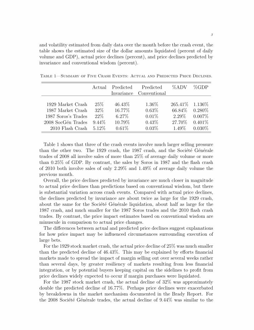
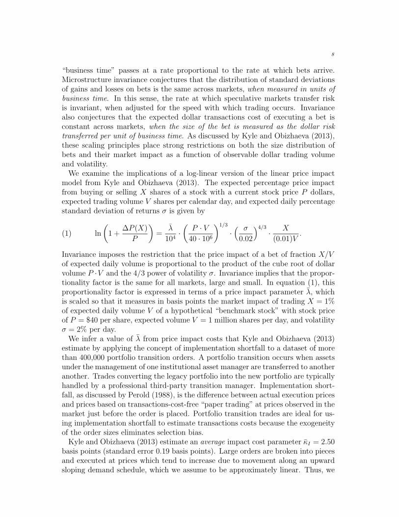
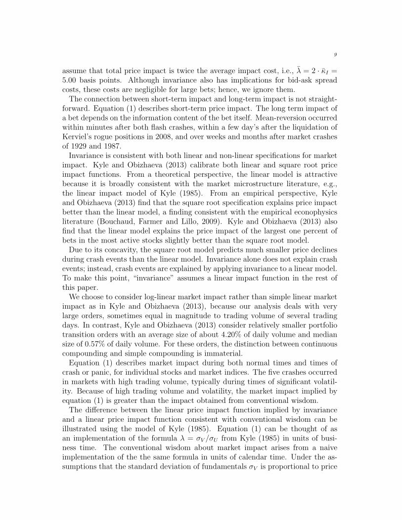
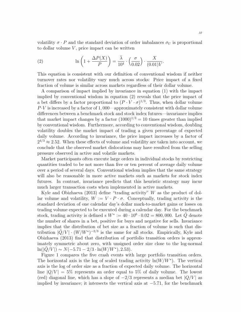
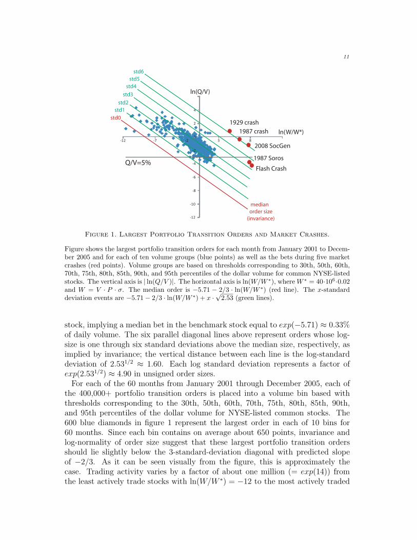
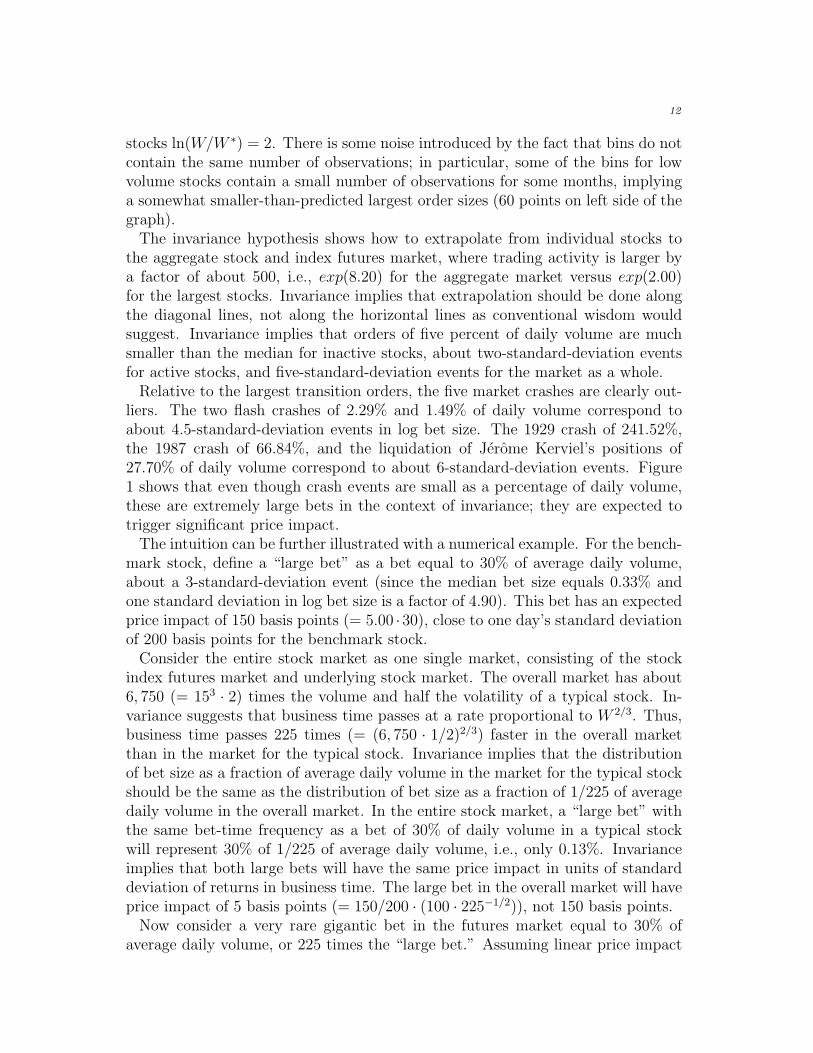
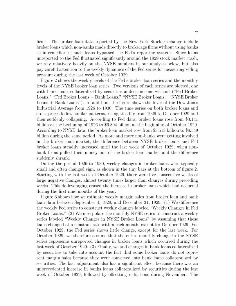
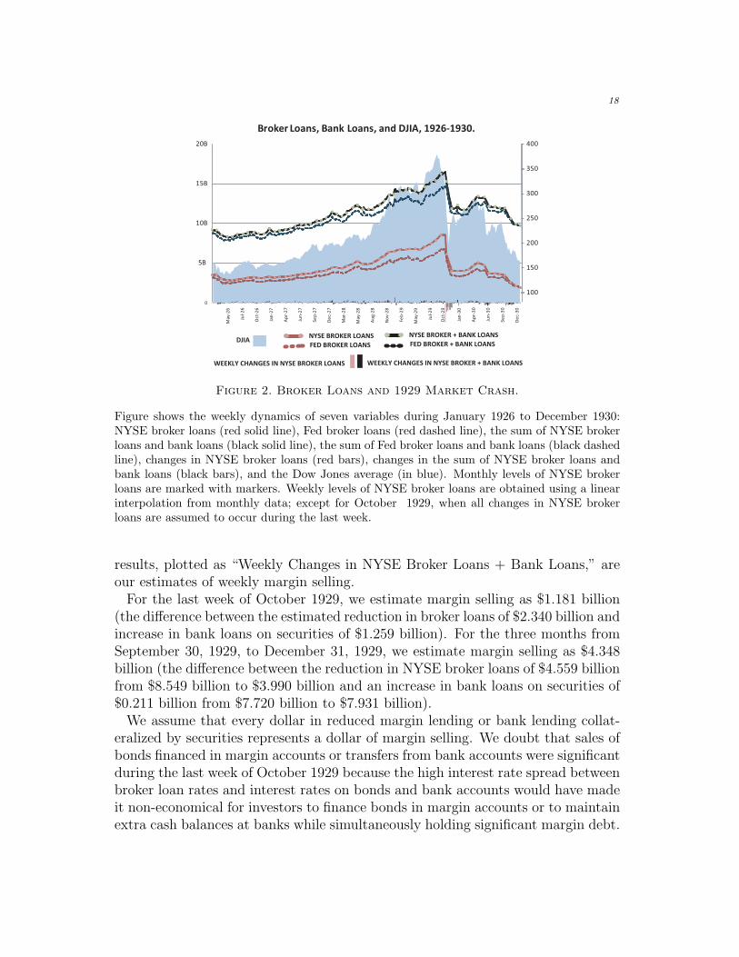
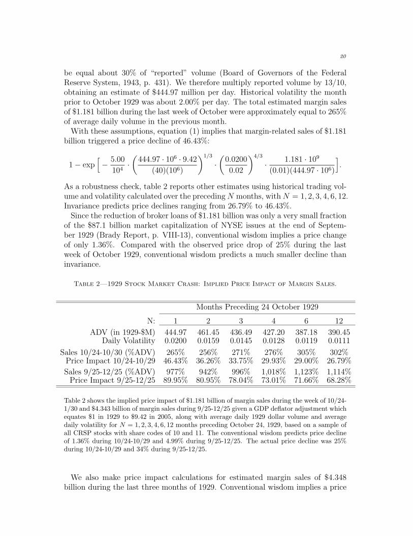
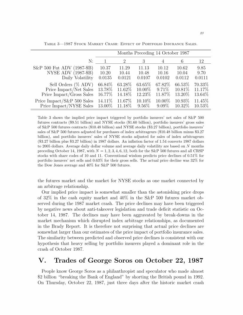
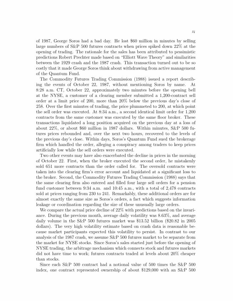
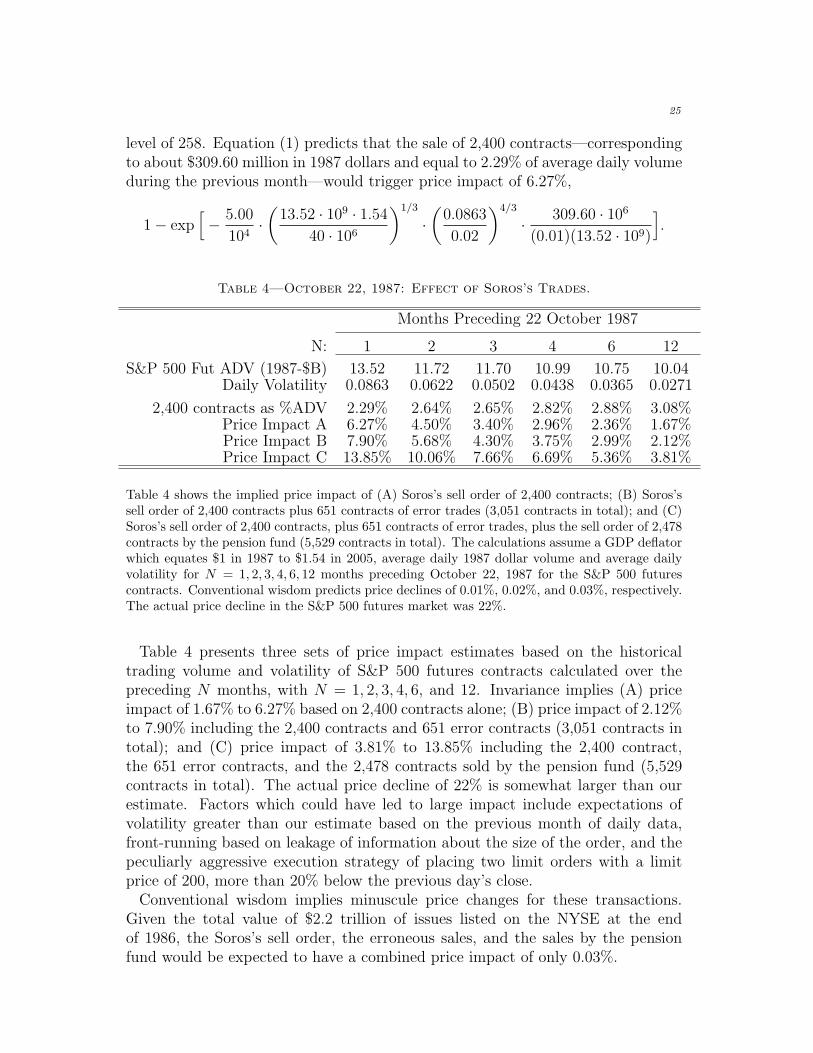
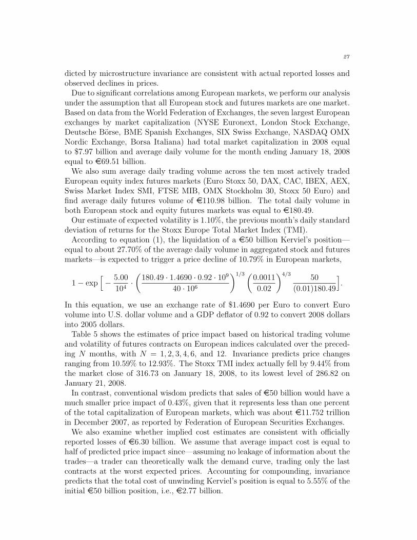
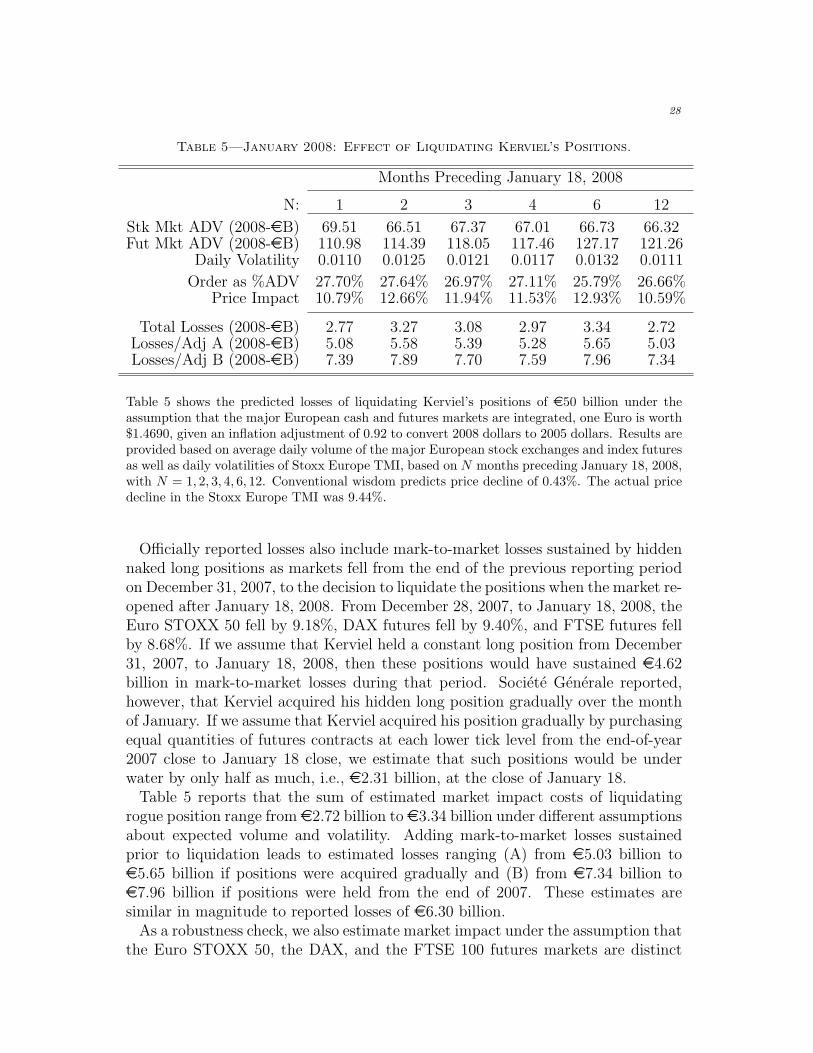
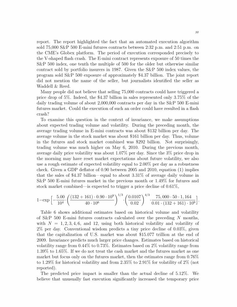


![Market Efficiency, Crashes, and Securities Litigationpeople.hss.caltech.edu/~bcornell/PUBLICATIONS/Market Efficiency... · 2006] MARKET EFFICIENCY 445 Although the Court confined](https://static.documents.pub/doc/80x56/5aed6bbb7f8b9a45568f9982/market-efficiency-crashes-and-securities-bcornellpublicationsmarket-efficiency2006.jpg)


