LDPC Codes Based on Latin Squares: Cycle Structure,

Stopping, and Trapping Set Analysis

Stefan Laendner and Olgica Milenkovic

Electrical and Computer Engineering Department

University of Colorado, Boulder, USA

Stefan.Laendner@colorado.edu and Olgica.Milenkovic@colorado.edu

Abstract

It is well known that certain combinatorial structures in the Tanner graph of a low-density

parity-check code exhibit a strong influence on its performance under iterative decoding. These

structures include cycles, stopping/trapping sets and parameters such as the diameter of the code.

In general, it is very hard to find a complete characterization of such configurations in an arbitrary

code, and even harder to understand the intricate relationships that exist between these entities. It

is therefore of interest to identify a simple setting in which all the described combinatorial structures

can be enumerated and studied within a joint framework. One such setting is developed in this

paper, for the purpose of analyzing the distribution of short cycles and the structure of stopping and

trapping sets in Tanner graphs of LDPC codes based on idempotent and symmetric Latin squares.

The parity-check matrices of LDPC codes based on Latin squares have a special form that allows

for connecting combinatorial parameters of the codes with the number of certain sub-rectangles

in the Latin squares. Sub-rectangles of interest can be easily identified, and in certain instances,

completely enumerated. The presented study can be extended in several different directions, one

of which is concerned with modifying the code design process in order to eliminate or reduce the

number of configurations bearing a negative influence on the performance of the code. Another

application of the results includes determining to which extent a configuration governs the behavior

of the bit error rate (BER) curve in the waterfall and error-floor regions.

1The results in this paper were presented in part at the IEEE International Conference on Communications, ICC’2004,Paris, France [14]. The work was supported in part by the NSF Grant CCF-0514921 and a fellowship by the Institute ofInformation Transmission (LIT) at the University of Erlangen-Nuremberg, Germany, awarded to Stefan Laendner.

1

Keywords: Cayley Latin Squares, Design Theory, LDPC Codes, Stopping Sets, and Trapping

Sets

1 Introduction

By now, it is well known that long random-like low-density parity-check (LDPC) codes used for sig-

nalling over discrete input memoryless channels have capacity-approaching performance under iterative

decoding [12]. Nevertheless, there still exist many open questions regarding the exact degree of influence

that specific parameters of a code exhibit on its overall performance when used for finite length data

transmission [20]. The best studied class of code parameters include the girth of a code [3], [4], [6], [7],

[9], [18] and the size of the smallest stopping set in the code graph [2], [15], but very few results are

available regarding trapping sets [13],[16] and pseudo-codewords [8]. Each of these entities can be used

individually in order to explain some phenomena underlying the behavior of the bit error rate (BER)

curve of a code under a given decoding strategy. For certain channels, like the binary erasure channel,

exact analytic characterizations of BER curves are possible in terms of the distribution of stopping set

sizes [2], [15]. What remains unknown is the exact nature of the relationship that exists between all the

aforementioned parameters and a study of their joint influence on the performance of LDPC codes in

channels like the additive white Gaussian noise (AWGN) channel.

The goal of this paper is to provide a comprehensive analysis of three different combinatorial param-

eters of a new class of LDPC codes based on idempotent and symmetric Latin squares. Such an analysis

is of importance in two different settings: in the first case, it allows for constructing large families of

high-rate codes with good performance under iterative decoding. In the second case, it can be used

as a starting point for investigating the influence of different classes of code parameters on the overall

performance of an LDPC code. The features analyzed include the structure and number of short cycles

in the Tanner graph and the size of the smallest stopping and trapping sets in the code graph. Although

stopping sets are primarily used for estimating the performance of LDPC codes over the binary erasure

channel, they are closely related to pseudo-codewords of many other channels [8] and are therefore of

interest when analyzing the performance of LDPC codes over the AWGN channel.

The codes described in this work are closely related to several other classes of LDPC codes based

on combinatorial designs. For a comprehensive treatment of the subject of LDPC code construction

2

based on design theory, the interested reader is referred to [6], [17], [18], [19], and the references therein.

The parity-check matrices of LDPC codes based on constrained Latin squares have a block structure

consisting of all-zero matrices and permutation matrices that are placed according to the entries in the

Latin square. If the squares are properly chosen, the resulting Tanner graphs of the codes have both

girth and minimum distance equal to six. The number of six-cycles and other short cycles in their

Tanner graph, as well as their stopping number and trapping set structures, can be determined in a

straightforward manner. This is due to the fact that the existence of stopping sets and trapping sets of

a prescribed size can be linked to the existence of sub-rectangles in the underlying Latin square. The

study of cycles, stopping and trapping sets reveals that most of these entities are related: for example,

the vertices corresponding to small stopping and trapping sets usually also belong to one or more short

cycles.

The outline of the paper is as follows. In Section 2 we introduce Latin squares, combinatorial

designs, and one-configurations [11]. We also describe several choices for Latin squares that result in

LDPC codes with good performance under iterative decoding. Section 3 is devoted to establishing a

relationship between stopping sets in LDPC codes and partial sub-rectangles of their corresponding

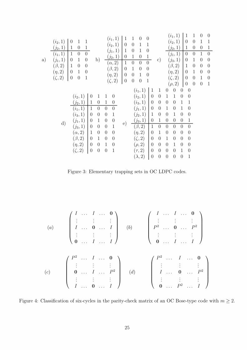
Latin squares. Section 4 contains a partial classification of elementary trapping sets in LDPC codes

based on symmetric, idempotent Latin squares, while Section 5 provides a count of the number of six-

cycles in the codes. Section 6 describes how some of the results in Section 5 can be used to improve

the performance of the codes in terms of a structured shortening procedure that reduces the number of

six-cycles in the code graph. Simulation results are given in Section 7.

2 Latin squares, designs and one-configurations

LDPC codes based on Latin squares were first described in [18], where Latin squares were first used

to construct Steiner triple systems and one-configurations. Such systems were subsequently used for

characterizing the parity-check matrix of LDPC codes. We start this section by providing the necessary

background needed for extending and generalizing this technique.

Definition 2.1. A Steiner 2-design is an ordered pair (V, B), where V is a set with v elements and B is

a collection of b subsets of size t over V , called blocks. Every element of V is contained in exactly t · b/v

blocks and every 2-subset of V is contained in exactly one block. A Steiner 2-design for which t = 3

3

is referred to as a Steiner triple system (STS). If the constraint of a 2-design is relaxed so that each

pair of elements in V is required to belong to at most one block, the resulting combinatorial structure is

called a one-configuration (OC).

An STS or OC can be used to define the parity-check matrix H of a LDPC code in a standard way:

the variables of the code correspond to blocks, while the parity-checks correspond to the points of the

system. In this case H represents the point-block incidence matrix of the given combinatorial objects

[18].

We will find the following definitions useful in the sequel of the paper.

Definition 2.2. A Latin square of order M is an M×M array such that each row and column contains

every symbol in 1, . . . , M exactly once. More generally, a Latin rectangle is an K × M, K ≤ M ,

matrix of entries with no symbol appearing more than once in each row and column. A Latin square is

idempotent if the cell indexed by (i, i), 1 ≤ i ≤ M , contains the symbol i, and symmetric if cells (i, j)

and (j, i), 1 ≤ i < j ≤ M , contain the same symbol.

Definition 2.3. If in a Latin square of order M , there exist r2 cells with r rows and r columns that form

a Latin square of order r and over an alphabet of size r, then these cells are said to form a sub-square

of order r. Similarly, a sub-rectangle of the Latin square is a sub-array of the square which is itself a

Latin rectangle. A Latin square of size M ×M is an N2 (N∞

) square if it does not contain sub-squares

of order two (of any order r > 1).

Of special interest for the derivations to follow are Cayley Latin squares, for which the entries are

determined by the Cayley table of the cyclic group of order m over the alphabet 1, . . . , M. More

specifically, the entry at position (i, j) in such a square is given by i + j − 1 mod M1. Equivalent to a

Cayley Latin square of odd order M under rearrangement of the rows, rearrangement of the columns,

or renaming of the symbols (i.e. isotopic to it) is a Latin square defined by the equation (i + j)/2

mod M . Cayley Latin squares of prime order q and Latin squares isotopic to them are examples of N∞

squares [1]. Throughout the rest of the paper we focus our attention on Latin squares with odd order

M = 2m + 1.

Definition 2.4. Let SQ be an idempotent and symmetric Latin square of order 2m + 1, let J =

1, 2, . . . , 2m + 1 and P = J × 1, 2, 3. Define a collection of blocks B that contains:1Here and throughout the rest of paper, we use the somewhat non-standard modulo function which assumes that the

symbol 0 is replaced by the symbol M .

4

a) all triples of the form (i, 1), (i, 2), (i, 3), where 1 ≤ i ≤ 2m + 1 (type 1 triplet);

b) all triples of the form (i, a), (j, a), (i j, b), a = 1, 2, 3, b = a + 1 mod 3, where 1 ≤ i < j ≤

2m + 1, and i j denotes the entry of the Latin square SQ in row i and column j (type 2 triplet).

It is straightforward to see that (P,B) is an STS with 6m + 3 points [11]. We will refer to such

an object as a Bose system. Observe that the symmetry of the underlying Latin squares leads to the

property that no two elements in row j and column j of that Latin square are the same, provided that

the positions are restricted to the “upper right triangle” of the square. Assume to the contrary that

i (i + 1) = (i + 1) (i + 2) = ℓ, i < m. Then there would exist two blocks in the Bose system of

the form (i, 1), (i + 1, 1), (ℓ, 2) and (i + 1, 1), (i + 2, 1), (ℓ, 2), containing the same pair of points and

hence violating the defining properties of an STS. If the square is symmetric, then i (i + 1) = ℓ, and

(i + 1) i = ℓ, so that (i + 1) (i + 2) 6= ℓ.

Claim 2.1. Let SQ be a symmetric and idempotent Latin square of order 2m+1 not divisible by seven,

with an entry in row i and column j chosen according to ij = (i+j)/2 mod (2m+1). The STS arising

from SQ does not contain a set of four blocks with six different points, i.e., a Pasch configuration.

LDPC codes derived from STSs free of Pasch configurations have minimum distance at least six [18].

Proof. In order to prove the claim, consider the following two properties of the square SQ: there are no

Latin sub-squares of order two contained within SQ (property P1) and there do not exist two different

integers x, y such that x (x (x y)) = y (property P2). The presence of a sub-square of order two

implies the existence of integers i 6= l and j 6= k such that i k = l j and i j = l k. Since the

order of the square is odd, this is impossible for the given construction since it leads to i = l and

k = j. The second property can be easily shown to be true by observing that for the given construction,

x (x (xy)) = y is equivalent to (7/8) x+(1/8) y = y, i.e. to 7 | 2m+1, which contradicts the starting

assumptions regarding the order of the Latin square.

We classify next the possible ways in which Pasch configurations resulting from type 1 and type 2

triplets may arise and show that a necessary condition for their existence is that either property P1 or

property P2 holds. Since neither of the two properties is satisfied for the described Latin squares, it

will follow that the STS based on SQ is Pasch-free.

1. A Pasch configuration cannot consist of more than one type 1 triplet; if there were at least

two type 1 triplets, say (x, 1), (x, 2), (x, 3), (y, 1), (y, 2), (y, 3), x 6= y, then these two triplets would

5

contain six different points, and it would be impossible to add one more triplet.

2. A Pasch configuration formed from type 2 triplets only may have blocks of the form:

(i, 1), (j, 1), (i j, 2), (i, 1), (k, 1), (i k, 2), (l, 1), (j, 1), (l j, 2), (l, 1), (k, 1), (l k, 2),

with i 6= l, j 6= k, i j = l k, and i k = l j; this is equivalent to property P1.

3. A Pasch configuration formed from type 1 and type 2 triplets has to be of the form:

(x, 1), (x, 2), (x, 3), (x, 1), (y, 1), (a, 2), (x, 2), (a, 2), (b, 3), (x, 3), (b, 3), (y, 1).

This implies that x y = a, x a = b, x b = y, i.e. x (x (x y)) = y, and is equivalent to property

P2.

Codes based on the described STS and codes based on an OC consisting of type 2 triplets only will be

referred to as STS LDPC and OC LDPC codes, respectively. For a Latin square of order 2m+1, the num-

ber of parity-checks for both STS and OC codes is v = 6m+3, while the number of variables in the first

case is (3m+1)(2m+1) = v(v−1)/6, and in the second case 3m(2m+1) = v(v−3)/6. The girth of the

code-graph is guaranteed to be six, since by the very definition of an STS (an OC system) every pair of

points belongs to exactly (at most) one block. Since the STS and OC systems described above are Pasch-

free, it follows that the resulting codes have minimum distance at least six. An STS code has minimum

distance exactly equal to six. This can be seen by considering the following set of six blocks from the STS,

three of which are of type 1 and three of which are of type 2: (x, 1), (x, 2), (x, 3),(y, 1), (y, 2), (y, 3),

(z, 1), (z, 2), (z, 3), (x, 1), (y, 1), (z, 2), (x, 2), (y, 2), (z, 3), (x, 3), (y, 3), (z, 1), where x, y, and z

are pairwise distinct and such that z = x y. These six blocks correspond to six variables, and the

points (l, k), l ∈ x, y, z and k = 1, 2, 3, correspond to nine different checks repeated exactly two times.

2.1 Parity-check matrices of codes based on Cayley Latin squares

Since for every type 2 triplet (i, a), (j, a), (i j, a + 1) in an STS or OC based on Latin squares there

also exist two “shifted” blocks (i, a + 1), (j, a + 1), (i j, a + 2) and (i, a + 2), (j, a + 2), (i j, a + 3)

with the values a, a+1, a+2, a+3 taken modulo 3, the parity-check matrix of the corresponding LDPC

codes can be decomposed into highly structured blocks of size three. This can be rigorously demonstrated

as follows. Let us label the points (i, a), 1 ≤ i ≤ 2m + 1, a ∈ 1, 2, 3 of the Bose STS and OC by

6

the integers 3 · (i − 1) + a. Additionally, let us index the blocks in such a way that type 1 triplets are

numbered according to the value i of the first coordinate of their points, and index the type 2 triplets

lexicographically but with all their shifts in consecutive order. In this setting, type 1 triplets introduce

2m+1 columns H(1) in the parity-check matrix H . These columns contain three consecutive ones in the

vertical direction as shown in Figure 1 a) for m = 2. Similarly, the sub-matrix H (2) of the parity-check

matrix H corresponding to type 2 triplets has a regular structure with 2m + 1 blocks of size three per

column and m(2m + 1) blocks of size three per row. By using the standard notation for the all-zero

matrix 0, identity matrix I and the basic circular permutation matrix P , the section H (2) of H for

m = 2 takes the form shown in Figure 1 b).

Let a column of blocks (matrices of size three) in H be called a block-column, and name the same

structure corresponding to rows a block-row. For example, in Figure 1 b), the stacked collection of blocks

(I I 0 P 2 0) represents a block-column. It is straightforward to see that H (2) can be partitioned into 2m

sub-matrices M1 M2 . . . M2m , where sub-matrix Mi, 1 ≤ i ≤ 2m, contains exactly 2m+1−i block-

columns. The structure of a sub-matrix can be described as follows: the i-th block-row of Mi consists

entirely of I matrices. Additionally, I matrices within Mi appear along the block-diagonal (i + l, l),

l ≥ 1. The positions of the permutation matrices P 2 can be determined from the description of the

Cayley Latin square: in block-column l of the sub-matrix Mi, P 2 is in block-row [(2i+l)/2] mod (2m+1)

if l is even, and in block-row [(2i+l+2m+1)/2] mod (2m+1) if l is odd. It suffices to construct only M1:

M2 can be obtained from M1 by retaining only the first 2m − 1 block-columns, and cyclically shifting

the block-rows. Similarly, Mi can be obtained from M1 by taking the first 2m + 1 − i block-columns

of M1 and shifting the block-rows cyclically by i − 1 positions. The matrix H (2) is regular in the sense

that there are exactly two I matrices and one P 2 matrix per block-column. Furthermore, the number

of P 2 and I matrices in H(2) per block-row is m and 2m, respectively.

Throughout the rest of the paper we focus our attention on analyzing OC LDPC codes and their

corresponding parity-check matrices. A similar study can be conducted for STS LDPC codes, and for

generalizations of OC codes resulting in LDPC codes of column weight four. These results will be

presented elsewhere.

7

3 Latin squares free of sub-squares and stopping sets in LDPC

codes

Based on the constructions outlined in the previous sections, it is straightforward to see that the presence

or absence of certain sub-configurations in the Latin square influences the characteristics of the Tanner

graph of the resulting code. For example, Pasch-free OCs based on Cayley Latin squares produce codes

of column-weight three with minimum distance at least six. Pasch configurations represent a special case

of a stopping set [2], [15]. A stopping set Σ of a code is a set of variables such that all checks connected to

Σ are connected to at least two different nodes in that set. The size of the smallest non-empty stopping

set of a parity-check matrix H is called the stopping number of H and it represents a lower bound for

the minimum distance of the code. The next results show that for OC LDPC codes there exists a more

general relationship between stopping sets and configurations in the underlying Latin squares.

Definition 3.1. A partial sub-rectangle of a Latin square is a partially or completely filled r × s sub-

array of not necessarily adjacent entries where each column and row contain at least two elements and

each entry appears at least twice in the array. The number of filled positions in a partial sub-rectangle

is called the size of the partial sub-rectangle and denoted by π. Clearly, π ≤ r · s. For completely filled

sub-squares and sub-rectangles one has π = r · s, and r, s ≥ 2.

It is straightforward to see that a partial sub-rectangle gives rise to a stopping set of size π in an

OC code. Furthermore, every stopping set corresponds to a partial sub-rectangle.

Lemma 3.1. An OC LDPC code constructed from a Latin square L of order 2m + 1 has no stopping

sets of size four if L ∈ N2, where N2 is defined as in Def. 2.3.

Lemma 3.2. If the Latin square contains a partial sub-rectangle of order r × 2, where r ≥ 2, then the

resulting OC LDPC code contains at least three stopping sets of size 2r.

Proof. A sub-rectangle of size r × 2 leads to a set of blocks of cardinality 2r, with each point contained

in the blocks appearing at least twice.

Theorem 3.3. If a Latin square of order 2m+1, used to construct an OC LDPC code according to the

Bose method, does not contain partial sub-rectangles of size π, then the stopping number of the code’s

(incidence) parity-check matrix H is at least π + 1.

8

Proof. The proof is a straightforward consequence of the previously described results.

It is known that Cayley Latin squares of odd prime order and squares isotopic to them have no

proper Latin sub-rectangles [21]. Therefore, π > 5 since there do not exist partial rectangles with

π = 5.

Theorem 3.4. Cayley Latin squares of prime order q ≥ 5 and squares defined by (i + j)/2 mod q

(which are isotopic to Cayley Latin squares) have point-block parity-check matrices with stopping number

σOC = 6.

Proof. First, recall that Cayley Latin squares are N∞

squares, so they do not contain proper Latin

sub-squares or sub-rectangles. Therefore, for π = 6 assume without loss of generality that the partial

sub-rectangle of interest is in one of the two staggered forms (S1) or (S2), with entries (α, β) or (α, β, η)

as shown below.

(S1)

j1 j2 j3

i1 ⋆ β α

i2 β α ⋆

i3 α ⋆ β

(S2)

j1 j2 j3

i1 ⋆ α β

i2 α ⋆ η

i3 β η ⋆

(1)

The defining equations for (α, β) in the (S1) structure read as

i1 + j3 − 1 = α,

i1 + j2 − 1 = β,

i2 + j2 − 1 = α,

i2 + j1 − 1 = β,

i3 + j1 − 1 = α mod q,

i3 + j3 − 1 = β mod q,(2)

where α 6= β, the values i1, i2, and i3 are pairwise distinct, and the same is true of j1, j2, and j3. A

suitable addition and subtraction of the six equations in (2) shows that the values of the parameters

α and β have to satisfy α = β mod q. But this is impossible, since both α and β are bounded from

above by q and by assumption α 6= β. It is straightforward to see that every Cayley Latin rectangle

9

must contain a partial sub-rectangle of the form (S2). An example for q = 7 is shown below.

1 2 3 4 5 6 7

2 3 4 5 6 7 1

3 4 5 6 7 1 2

4 5 6 7 1 2 3

5 6 7 1 2 3 4

6 7 1 2 3 4 5

7 1 2 3 4 5 6

(3)

Codes based on Cayley Latin squares also contain stopping sets of size seven. This can be seen based

on the two possible structures 2 for partial rectangles of the forms (D1), (D2) shown below:

(D1)

j1 j2 j3

i1 η β α

i2 β α ⋆

i3 ⋆ η β

(D2)

j1 j2 j3

i1 ⋆ β α

i2 β α η

i3 α η ⋆

It is straightforward to see that type (D1) partial rectangles exist in Cayley Latin squares. Type (D2)

partial rectangles with j3 = j2 +1 = j1 +2, i3 = i2 +1 = i1 +2 are also present in Cayley Latin squares,

which is a simple consequence of the defining equation for these Latin squares.

The structures of the stopping sets corresponding to sub-rectangles of the form (S2), (D1) and (D2) are

shown in Figure 2. The stopping sets induced by (S2) sub-rectangles define a codeword, while those

induced by (D1) and (D2) do not correspond to codewords. Furthermore, each of the stopping sets

shown in Figure 2 contain short cycles: the (S2) structure contains both an eight- and a twelve-cycle,

while both (D1) and (D2) contain exactly six six-cycles.

2or a transpose/symbol permutation/symbol reassignment thereof

10

4 Sub-squares of Latin squares and trapping sets in OC LDPC

codes

We discuss next the relationship between the structure of trapping sets [13], [16] in the code graph

of an OC LDPC code and partial sub-rectangles in the corresponding Latin square. We restrict our

interest to elementary trapping sets which are defined as subsets of variable nodes of the code graph

with the property that their induced subgraph contains check nodes of degree one and two only [10].

If an elementary trapping set contains Ω variables and Θ check nodes of degree one, then it is said to

have parameters (Ω, Θ). Certain classes of elementary trapping sets are known to contribute to the

emergence of high error floors in BER curves of codes used over the AWGN channel [13], [16].

For OC LDPC codes, the constraint on the structure of an elementary trapping set translates to the

requirement that in a sub-rectangle of the underlying Latin square each symbol appears at most twice

and that each row in the partial rectangle contains at most two entries. Equivalently, any collection

of type 2 triplets containing the same point at most twice corresponds to an elementary trapping set.

It is straightforward to see that OC LDPC codes contain (2, 5) and (2, 6) trapping sets. We focus on

trapping sets for which Ω ≥ 3. There exist many possible structures for partial rectangles satisfying the

previously described constraints, five of which are shown below.

(T1)

j1 j2

i1 ⋆ β

i2 η ζ

(T2)

j1 j2

i1 α β

i2 η ζ

(T3)

j1 j2 j3

i1 ⋆ β η

i2 ζ ρ ⋆

(T4)

j1 j2 j3

i1 ⋆ α ⋆

i2 β η ⋆

i3 ⋆ ⋆ ζ

(T5)

j1 j2 j3

i1 ⋆ β η

i2 ζ ρ ⋆

i3 τ ⋆ λ

The sub-rectangles (T1), (T2), (T3), (T4) and (T5) involve a small number of variables and hence corre-

spond to trapping sets with small values of Ω. The parameter Θ of the trapping sets depends on the

relationship between the values of the elements in α, β, . . . , ζ.

Sub-squares of the form (T1) induce the following set of three blocks in the corresponding OC:

(i1, 1), (j2, 1), (β, 2), (i2, 1), (j1, 1), (η, 2), (i2, 1), (j2, 1), (ζ, 2).

11

For β 6= η the resulting configuration represents a (3, 5) trapping set, shown in Figure 3 a). Other-

wise, it represents a (3, 3) trapping set, since in this case two rows of weight one in a (3, 5) trapping set

have to be merged into a row of weight two. Observe also that since it must hold that η 6= ζ and β 6= ζ ,

no (3, 2) elementary trapping sets can arise from a sub-rectangle of type (T1). This is due to the fact

that the three points (i1, 1), (j1, 1) and (ζ, 2) all appear exactly once in the blocks (4).

Partial sub-squares of the form (T2) result in the following set of three blocks:

(i1, 1), (j1, 1), (α, 2), (i1, 1), (j2, 1), (β, 2), (i2, 1), (j1, 1), (η, 2), (i2, 1), (j2, 1), (ζ, 2).

This set of blocks represents a (4, 4) elementary trapping set shown in Figure 3 b), provided that

α 6= ζ and β 6= η. If either α = ζ or β = η, but not both equalities are simultaneously true, the

resulting configuration is a (4, 2) elementary trapping set. It is straightforward to see that type (T2)

sub-rectangles with both set of parameters described above exist in a Cayley Latin square. On the other

hand, sub-rectangles with α = ζ and β = η do not exist in Cayley Latin squares. Consequently, OC

LDPC codes based on Cayley Latin squares contain (4, 2) and (4, 4) elementary trapping sets, but they

do not contain (4, 0) trapping sets - i.e. they do not contain codewords of weight four.

Partial sub-rectangles of type (T3) produce the following four blocks:

(i1, 1), (j2, 1), (β, 2), (i1, 1), (j3, 1), (η, 2), (i2, 1), (j1, 1), (ζ, 2), (i2, 1), (j2, 1), (ρ, 2)

Provided that β 6= ζ , η 6= ζ , and η 6= ρ, the resulting configuration is a (4, 6) elementary trapping

set shown in Figure 3 c). If β = ζ or η = ρ, but not both equalities are simultaneously true, the

sub-rectangle induces a (4, 4) trapping set. Finally, if β = ζ and η = ρ the OC LDPC code contains

(4, 2) trapping sets.

Partial sub-rectangles of type (T4) produce the following four blocks:

(i1, 1), (j2, 1), (α, 2), (i2, 1), (j1, 1), (β, 2), (i2, 1), (j2, 1), (η, 2), (i3, 1), (j3, 1), (ζ, 2)

Provided that the parameters α, β, η and ζ take distinct values, the resulting configuration reduces to

a (4, 8) elementary trapping set shown in Figure 3 d). If ζ = η and α 6= β, the resulting configuration

corresponds to a (4, 6) elementary trapping set. For ζ = η and α = β, a (4, 4) trapping set is introduced

into the code graph.

12

Partial sub-rectangles of the form (T5) induce the following set of four blocks

(i1, 1), (j2, 1), (β, 2), (i1, 1), (j3, 1), (η, 2), (i2, 1), (j1, 1), (ζ, 2),

(i2, 1), (j2, 1), (ρ, 2), (i3, 1), (j1, 1), (τ, 2), (i3, 1), (j3, 1), (λ, 2).

Provided that β 6= ζ , ζ 6= η, ζ 6= λ, τ 6= β, τ 6= η, and τ 6= ρ, the configuration of blocks described

above produces a (6, 6) elementary trapping set shown in Figure 3 e). If exactly one of the equalities

β = ζ, ζ = η, ζ = λ, τ = β, τ = η, and τ = ρ

is satisfied, the configuration (T4) induces a (6, 4) elementary trapping set. If η = ρ = τ , then one parity-

check in the induced graph has degree three, and consequently the configuration does not correspond

to an elementary trapping set. If β = ζ and in addition, one of the equalities η = ρ, η = τ , or ρ = τ is

true, then the resulting configuration corresponds to a (6, 2) trapping set. By setting β = ζ , η = τ , and

λ = ρ one obtains a stopping set corresponding to a codeword of weight six.

Similarly to stopping sets, the trapping sets described above also contain embedded cycles. For

example, a type (T2) set with α 6= ζ, β 6= η contains an eight cycle involving all checks of degree two,

as can be seen from Figure 3 b). For the case that β = η or α = ζ , but not both are simultaneously

true, the resulting trapping set contains a six-cycle. Similarly, for type (T5) sets, either a six-cycle,

eight-cycle or 12-cycle are present in the code graph, depending on the relationship between the entries

in the corresponding sub-rectangle of the Latin square.

5 Classification of Six-Cycles

We conduct next a classification of six-cycles in OC LDPC codes. It suffices to first identify all block-

cycles, representing special closed paths formed by the size three I and P 2 matrices. To make the notion

of a block-cycle more rigorous, we need the following lemma from [4].

Definition 5.1. Let an LDPC code be defined by a parity-check matrix consisting of glued permutation

blocks P ij of order D, for some set ij of non-negative integers. The Fan sum is defined as i1 − i2 +

i3 − i4 + · · · + i2l−1 − i2l mod D, where ij, j = 1, . . . , 2l denote the cyclic offsets of the permutation

matrices encountered in a closed path of length 2l within the parity-check matrix.

13

Lemma 5.1. The parity-check matrix of an LDPC code consisting of glued permutation blocks P ij of

order D, for some set ij of non-negative integers contains cycles of length 2l provided that there exist

non-negative integers i1, . . . , i2l such that their Fan sum is identically equal to zero.

A block-cycle can now be defined as a closed path involving non-zero blocks in the parity-check

matrix for which the corresponding Fan sum equals zero. A block-cycle with exactly six blocks will be

denoted by C6.

Consider an OC LDPC code involving type 2 triplets only. In this case, a C6 cycle can occur for

the following patterns of I and P 2 matrices listed below. Note that whenever allowed by the structure,

block-rows and block-columns can be arbitrarily permuted.

Class (a): Only I matrices participate in the formation of a block-cycle (Figure 4 a)). In order

to construct a six-cycle including only I matrices, one needs two pairs of I matrices from two different

block-columns of one sub-matrix Mi, and one block-column from a sub-matrix Mj, j 6= i. Since the

block-column from Mj is uniquely determined by the choice of the first two block-columns, one has

exactly(

2m+1−i2

)

possible C6 cycles for a pair of columns chosen from the matrix Mi. The total number

na of block-cycles of this type is equal to

na =2m−1∑

i=1

(

2m + 1 − i

2

)

=m

3(4m2 − 1).

Observe that the largest number of block-cycles of this form is contained in M1.

Class (b): Two P 2 matrices within the same block-row participate in the formation of a six-cycle

(Figure 4 b)). For each pair of P 2 matrices in one block-row, there are exactly four possible C6 cycles,

since for every P 2 there are two choices for the I matrix in the same block-column. Hence, since there

are m matrices P 2 per row, one has(

m2

)

pairs of I matrices to choose from. This results in

nb = 4 ·

(

m

2

)

· (2m + 1) = 2 · (2m + 1) · m(m − 1)

C6 cycles of the above described form.

Class (c): Two P 2 matrices in two different block-rows, connected through a pair of I matrices,

are part of this type of C6 cycle (see Figure 4 c)). Note that in order to close the cycle, one must also

include two I matrices. A C6 cycle consisting of two P 2 matrices connected by a pair of I matrices

14

can be formed by starting from any P 2 matrix, and then choosing one out of exactly two I matrices

within the same block-column. After that, there are 2m − 1 choices for another I matrix within the

same block-row. The P 2-matrix in the corresponding column is unique, as well as the “closing path” of

the C6 cycle by a pair of I matrices (having the same row indices as the two P 2 matrices). In this way

each C6 cycle is counted exactly twice. Therefore,

nc = 2 · (2m − 1) · m(2m + 1)/2 = m(4m2 − 1).

Class (d): Exactly one P 2 matrix per block-row and per block-column participates in the cycle (see

Figure 4 d)). For each P 2 matrix one can form a C6 cycle of this type from three I and three P 2 matrices.

Starting from any P 2 matrix, one can choose one out of two I matrices in the same block-column for

the second point in the block-cycle. Afterwards, one can choose freely any of the m P 2-matrices in the

corresponding block-row. Finally, there is at least one and at most two choices for the next I matrix.

This is due to the following fact. The two I matrices and the unique P 2 matrix in block Mi and within

block-column j are in block-rows i, i + j and (2i + j)/2 mod (2m + 1), respectively. Once three of

the matrices are fixed as described above, there is a unique choice for a pair of block-columns with the

specified coordinates. But the second chosen I matrix may belong to the same block-row as the initially

chosen P 2 matrix, in which case no C6 cycle can be completed. If a cycle can be completed, the last

matrix in the block-cycle is uniquely determined by the previous choices. Due to the regularity of the

construction, the number of C6 cycles of this type is the same for all choices of P 2 matrices. Hence,

nd ≥ m(2m + 1) · 2m/3 = 2 · m2(2m + 1)/3, and nd ≤ 4 · m2(2m + 1)/3,

since it is not possible to determine exactly if one or two choices for the second I matrix are possible.

The count above shows that the number of C6 cycles of an OC LDPC code is at least

m

3

(

32m2 − 4m − 10)

i.e. O(m3). The actual number of cycles in the bipartite graph can be obtained by multiplying the total

number of C6 cycles by three.

15

6 Applications of cycle-enumeration techniques

The results of the analysis presented in Section 3, 4, and 5 can be used to modify the OC LDPC

code design process in order to eliminate some undesired cycles, stopping or trapping sets. Due to

space limitations, we will focus only on methods aimed at decreasing the number of six-cycles. Two

such methods are described in Section 6.1 and Section 6.2, were the parity-check matrix of an OC

code is restructured in terms of increasing the size of its permutation blocks or deleting some of its

block-columns.

6.1 Modifications of the parity-check matrix of OC LDPC codes

Based on the classification of cycles described in Section 5, we show next how to eliminate the class (d)

C6 cycles by simply increasing the dimension of the permutation blocks and all-zero matrices. Increasing

the dimension will result in the same number of block-cycles but more cycles of class (a), (b) and (c)

will emerge. The increase in the number of class (a), (b) and (c) cycles will be compensated by the

decrease in type (d) cycles.

Lemma 6.1. Assume that the parity-check matrix of an OC LDPC code is modified by changing the

order of all its sub-matrices from three to five. Then the OC LDPC code contains no C6 block-cycles

of type d), and no additional C6 block-cycles nor block-cycles of length four are introduced into the code

graph.

Proof. For the case of class (a), (b) and (c) C6 cycles, the Fan sum is identically equal to zero, since all

positive terms in the sum are cancelled out. Only for the class (d) block-cycles does the Fan sum equal

to −6 = 0 mod 3. If one increases the size of the blocks in the parity-check matrix of such codes to

D = 5, the Fan sum cannot take the values −5 or 5, since all its summands are even. Hence, the sum

must have absolute value equal to 10. This implies that at least five P 2 matrices are encountered on

such a path, which is impossible based on the fact that every block-column of the parity-check matrix

contains at most one P 2 matrix. Furthermore, the increase of the block-size to D = 5 does not introduce

a block-cycle of length four, since the maximum Fan sum for a block-cycle of length four has to have

absolute value 8. This completes the proof.

We will refer to the technique described in lemma 6.1 as the order modification method. It can be easily

shown that an OC LDPC code constructed according to the order modification method, for sufficiently

16

large m, has a twelve times smaller number of cycles of length six then a code of the same length

constructed according to the standard Bose method.

6.2 Structured removal of six-cycles

We show next how to shorten OC LDPC codes so as to decrease the total number of six-cycles in their

Tanner graphs. An analysis similar to the one described below can also be performed for other cycle

lengths.

It is straightforward to see that removing the first block-column in block M1 of the parity-check

matrix eliminates at least

• 2m − 1 class (a) block-cycles of length six that contain the first block-column;

• 4 · (m − 1) block-cycles of length six formed by the P 2 matrix in the removed block-column and

another P 2 matrix within the same block-row;

• 2 · (2m− 1) block-cycles of length six formed by the P 2 matrix in the removed block-column and

an additional P 2 matrix, connected through a pair of I matrices;

• 4 · m block-cycles of length six formed by the P 2 matrix within the removed block-column and

two other P 2 matrices within two different block-columns.

Let us assume that we removed j − 1 block-columns from Mi, starting from the leftmost position.

Removing the j-th leftmost block-column results in breaking up 2m− i− j +1 block-cycles of class (a).

The number of block-cycles of class (b), (c), (d) that are broken by removing the j-th column depends

on how many and which columns are removed from other blocks. One can observe that the number

of class (a) cycles eliminated by the procedure described above depends only on the sum of the block

index i and the index j of the block-column within its corresponding Mi sub-matrix. This, of course,

is true only if the first j − 1 block-columns in Mi were already removed. Consequently, the removal

of the jth block-column in Mi breaks as many class (a) block-cycles as the removal of the (j − 1)th

block-column from the sub-matrix Mi+1. One way to perform structured removal of block-columns is

to delete the first s block-columns from block M1, the first s − 1 block-columns from block M2,..., and

one block-column from Ms, for some fixed value s. This process results in the most simple parity-check

matrix structure, and it leads to shortened codes with very good performance. The integer value s can

be chosen in such a way as to achieve a desired rate for the code.

17

Theorem 6.2. Let s = m − 1 be an even integer. Then the number of class (a) and (b) block-cycles

after the removal of the first s block-columns from M1, the first s − 1 block-columns from M2,..., the

first block-column from Ms−1, equals

2(2m + 1)

3

(

m + 1

2

)

, and 16

(

m

2

)

+ 16

(

(3m − 5)/2

2

)

+ 12

(

(m + 1)/2

2

)

,

respectively.

Proof. In order to find the number of block-cycles of a given class after block-column removal, one has

to first count how many I and how many P 2 matrices are erased from each of the block-rows. It is

straightforward to see that s identity matrices I are removed from each block-row indexed by t, where

1 ≤ t ≤ s + 1. Since the position of a P 2 matrix within the jth block-column is uniquely determined,

one can obtain the following distribution for deleted P 2 blocks, which holds for s ≤ m−1. The notation

BR is reserved for the index of the block-row, and N for the number of deleted P 2 matrices.

BR 2 3 . . . s/2 + 1 s/2 + 2 s/2 + 3 . . . s

N 1 2 . . . s/2 s/2 − 1 s/2 − 2 . . . 1

m + 2 m + 3 . . . m + s/2 m + s/2 + 1

1 2 . . . s/2 − 1 s/2

BR m + s/2 + 2 m + s/2 + 3 m + s/2 + 4 . . . m + s m + s + 1

N s/2 s/2 − 1 s/2 − 2 . . . 2 1

For block-row indices BR not listed above, the number of deleted P 2 matrices is zero. This shows that

the number of class (a) block-cycles after block-column removal equals

(s + 1)

(

2m − s

2

)

+2m−1∑

i=s+1

(

2m − i + 1

2

)

= (s + 1)

(

2m − s

2

)

+

(

2m − s + 1

3

)

.

By replacing s = m − 1, the above expression reduces to the result claimed in the statement of the

theorem. One can also show that the number of class (b) block-cycles after block-column removal equals

4

4

s/2−1∑

i=1

(

m − i

2

)

+ 3

(

m − s/2

2

)

+ 2

(

m

2

)

(m − s + 1)

.

18

The last expression is a consequence of the fact that in exactly four block-rows we erased p permutation

matrices P 2, for p = 1, . . . , s/2−1, and in exactly three block-rows we erased s/2 permutation matrices

P 2. No P 2 matrices are erased in the remaining 2(m− s + 1) block-rows. Substituting s = m− 1 gives

the desired result.

Remark 6.3. Note that there does not seem to be a simple method for counting the number of class (c)

and (d) block-cycles after structured column removal of the form described in theorem 6.2.

7 Simulation Results

The performance of several high-rate STS and OC LDPC codes based on Cayley Latin squares used

over the AWGN channel is shown in Figures 5, 6, and 7. Observe that the rate of a code is denoted

by R, and that the parameters of the code are given in terms of (n, k), where n denotes the length,

and k the dimension of the code. The performance of codes obtained by structured shortening and

codes derived from the order modification method are evaluated as well. The plots are obtained by

Monte Carlo simulations with 50 iterations of the message passing algorithm and with 10000 − 100000

codeword blocks. All the bit-error-rate (BER) curves are compensated for their respective rate loss,

i.e. the signal-to-noise ratio is computed according to SNR = 10 log10(Eb/N0) = 10 log10(1/(2Rσ2N))

from the rate and the noise standard deviation of the AWGN channel. As can be seen from Figures

5 and 6, Cayley Latin square codes have performance almost identical to that of random-like codes of

comparable length and rate, constructed by MacKay, (see www.inference.phy.cam.ac.uk/mackay/).

The OC LDPC codes in Figures 5 and 6 are generated based on the Bose construction method with

parameter m as described in Section 2.1, and using only type 2 triplets. The resulting code parameters

are equal to n = 3m(2m+1) and k = 3m(2m+1)−6m−3. Structured shortening is performed for the

codes by removing block-columns from their parity-check matrices according to the strategy described in

Section 6.2: the first s block-columns are removed from block M1, the first s−1 block-columns from M2,

etc., and the first block-column is removed from block Ms. Overall, the code is shortened by 3s(s+1)/2

columns and has length n = 3m(2m + 1)− 3s(s + 1)/2 and dimension k = 6m2 − 3m− 3− 3s(s + 1)/2.

Figure 5 shows the performance of codes of length approximately 1000. The first curve corresponds

to the (1053, 972) OC LDPC code, constructed from a Cayley Latin square with m = 13, rate R = 0.923

and with no columns removed (s = 0). The (1026, 897) code with rate R = 0.874 is constructed from

19

a Cayley Latin square with m = 21 and s = 33, by removing exactly 1683 columns. Compared to

MacKay’s (999, 888) random code of rate R = 0.889, the (1026, 897) code shows almost no performance

loss.

Figure 6 shows a comparison of several codes of length around 4400. The code with parameters

(4455, 4290) of rate R = 0.963 is generated from a Cayley Latin square with m = 27, for which one has

s = 0. The (4350, 4137) code of rate R = 0.951 is generated from a Cayley Latin square with m = 35

and s = 45, so that 3105 columns are removed from the original code. The third code with dimensions

(4455, 4032), generated from a Cayley Latin square with m = 70 and s = 129, results in a rate R = 0.905

code. These codes are compared to MacKay’s (4376, 4095) random code of rate R = 0.936. As can be

seen, the shortened codes show a competitive performance up to a bit error rate of 10−5.

Figure 7 shows the effect of modifications of the parity-check matrix of OC LDPC codes, namely the

order modification method , described in Section 6.1. The figure shows Bose LDPC codes generated by

Steiner triple systems having sub-matrices of order three, denoted by “dim3”, as well as their counterpart

OC LDPC codes of increased block-size D = 5, denoted by “dim5”. The increase in dimension is

achieved by replacing all order three I and P 2 matrices in the parity-check matrices of the Bose LDPC

codes (with the structure shown in Figure 1 b)) by corresponding I and P 2 matrices of order five. No

shortening of the original parity-check matrix was performed for these test-codes.

The (4134, 3975) dim3 code and the (6890, 6500) dim5 code, both of rate R = 0.962, are constructed

from a Cayley Latin square with parameter m = 26, the (2709, 2580) dim3 and the (4515, 4200) dim5

code of rate R = 0.952 are generated from a Cayley Latin square with m = 21. Furthermore, the

(759, 690) dim3 code and the (1265, 1100) dim5 code have rate R = 0.909 and are generated from

a Cayley Latin square with parameter m = 11. The plot shows the effect of the increased order of

the submatrix reducing the number of block cycles of type (d) (see Section 6.1) without introducing

shorter-length cycles. For Eb/N0=5.5dB, it can be seen that the dim5 codes clearly outperform their

dim3 counterparts.

Additionally, Monte Carlo simulations performed on the (1053, 972) OC LDPC code with parameter

m = 13 revealed that for high SNR values, most error patterns not corrected after 200 iterations

of belief propagation correspond to elementary trapping sets. An analysis of error-frames at 6.5 dB

for the decoder implementation A2 described in [10] showed that sets of variables corresponding to

(3, 5) trappings sets of type (T1) were frequently in error. The channel outputs for the three variables

20

in the trapping sets were strongly biased towards the wrong decision and an interesting “oscillation

phenomena” was detected. At every even iteration, the set of variable nodes in error corresponded to

a (3, 5) trapping set, while the set of variables in error at odd iterations usually included more than

200 variable nodes. Other types of elementary trapping sets detected during decoding include the (T5)

configuration corresponding to a (4, 8) trapping set.

Acknowledgment: The authors are grateful to the anonymous reviewers for very helpful and

insightful comments that largely improved the presentation of the results in the paper and the quality

of the exposition.

References

[1] J. Denes and A. Keedwell, Latin squares: New developments in the theory and applications, Chapter

4 by K. Heinrich, Annals of Discrete Mathematics, vol. 46, North Holland Publishing Company,

1991.

[2] C. Di, D. Proietti, I. E. Telatar, T. Richardson, and R. Urbanke, “Finite-length analysis of low-

density parity-check codes on the binary erasure channel,”IEEE Trans. on Inform. Theory, vol. 48,

no. 6, pp. 1570-1579, June 2002.

[3] I. Djurdjevic, J. Xu, K. Abdel-Ghaffar, and S. Lin, “A class of low-density parity-check codes

constructed based on Reed-Solomon codes with two information symbols,” IEEE Comm. Letters,

vol. 7, pp. 317-319, July 2003.

[4] J. L. Fan, “Array codes as LDPC codes,” in Proc. 2nd Int. Symp. Turbo Codes and Related Topics,

pp. 553-556, Brest, France, September 4–7, 2000.

[5] F. Lazebnik and V. Ustimenko, “Explicit construction of graphs with arbitrary large girth and of

large size,” Discrete Applied Mathematics, vol. 60, pp. 275-284, 1997.

[6] S. J. Johnson and S. R. Weller, “Regular low-density parity-check codes from combinatorial de-

signs,” Proceedings of the 2001 IEEE Information Theory Workshop, pp. 90-92, Australia, 2001.

21

[7] J. L. Kim, U. Peled, I. Perepelitsa, V. Pless, and S. Friedland, “Explicit construction of families of

LDPC codes with no 4-cycles,”IEEE Trans. on Info. Theory, vol. 50, no. 10, pp. 2378 - 2388, Oct.

2004.

[8] R. Koetter and P. O. Vontobel, “Graph covers and iterative decoding of finite-length codes,”

Proc. 3rd International Symposium on Turbo Codes and Related Topics, Brest, France, pp. 75-82,

September 2003.

[9] Y. Kou, S. Lin, and M. Fossorier, “Low-density parity-check codes based on finite geometries: a

rediscovery and new results,” IEEE Trans. Inform. Theory, vol. 47, pp. 2711-2736, November 2001.

[10] S. Laendner and O. Milenkovic, “Algorithmic and combinatorial analysis of trapping sets in struc-

tured LDPC codes,” Proceedings of WirelessCom 2005, Hawaii, June 2005.

[11] C.C. Lindner and C.A. Rodger, Design theory, CRC Press 1997.

[12] http://www.inference.phy.cam.ac.uk/mackay/CodeFiles.html

[13] D. MacKay, and M. Postol, “Weaknesses of Margulis and Ramanujan-Margulis low-density

parity-check codes,” Electronic Notes in Theoretical Computer Science, vol. 74, 2003, URL:

http://www.elsevier.nl/locate/entcs/volume74.html.

[14] O. Milenkovic and S. Laendner, “Analysis of the cycle structure of LDPC codes based on Latin

squares,” IEEE International Conference on Communications, ICC’2004, vol. 2, pp. 777-781, Paris,

June 2004.

[15] A. Orlitsky, R. Urbanke, K. Viswanathan, and J. Zhang, “Stopping sets and the girth of Tanner

graphs,” Proceedings of the ISIT’2002, Lausanne, Switzerland, p. 2, June/July 2002.

[16] T. Richardson, “Error-floors of LDPC codes,” Proceedings of the 41st Annual Allerton Conference

on Communication, Control and Computing, pp. 1426–1435, September 2003.

[17] B. Vasic, E. Kurtas, A. Kuznetsov, and O. Milenkovic, Structured low-density parity-check codes,

in Coding and Signal Processing for Magnetic Recording Systems, Editors B. Vasic and E. Kurtas,

CRC Press, 2005.

22

[18] B. Vasic and O. Milenkovic, “Combinatorial constructions of low-density parity-check codes for

iterative decoding,” IEEE Trans. on Inform. Theory, vol. 50, no. 6, pp. 1156-1177, June 2004.

[19] B. Vasic, E. Kurtas, and A. Kuznetsov,“LDPC codes based on mutually orthogonal Latin rectangles

and their applications in perpendicular magnetic recording,” IEEE Trans. on Magnetics, vol. 38,

no. 5, Part I, pp. 2346-2348, September 2002.

[20] P. O. Vontobel and R. Koetter, “On the Relationship between linear programming decoding and

min-sum algorithm decoding,” Proc. ISITA 2004, Parma, Italy, p. 991-996, October 2004.

[21] I.M. Wanless, “Perfect factorizations of bipartite graphs and Latin squares without proper subrect-

angles,” Electron. J. Combin., vol. 6, R9, 16 pp., 1999.

23

a) H(1) =

0 0 0 0 0 0 0 0 0 0 0 0 1 1 10 0 0 0 0 0 0 0 0 1 1 1 0 0 00 0 0 0 0 0 1 1 1 0 0 0 0 0 00 0 0 1 1 1 0 0 0 0 0 0 0 0 01 1 1 0 0 0 0 0 0 0 0 0 0 0 0

T

b) H(2) =

I I I I 0 0 P 2 P 2 0 0I P 2 0 0 I I I 0 0 P 2

0 I 0 P 2 I P 2 0 I I 0P 2 0 I 0 0 I 0 I P 2 I0 0 P 2 I P 2 0 I 0 I I

Figure 1: Structure of the parity-check matrix of an OC Bose-type code with m = 2.

(S2):

(i1, 1) 1 1 0 0 0 0(i2, 1) 0 0 1 1 0 0(i3, 1) 0 0 0 0 1 1(j1, 1) 0 0 1 0 1 0(j2, 1) 1 0 0 0 0 1(j3, 1) 0 1 0 1 0 0(α, 2) 1 0 1 0 0 0(β, 2) 0 1 0 0 1 0(η, 2) 0 0 0 1 0 1

(D1):

(i1, 1) 1 1 1 0 0 0 0(i2, 1) 0 0 0 1 1 0 0(i3, 1) 0 0 0 0 0 1 1(j1, 1) 1 0 0 1 0 0 0(j2, 1) 0 1 0 0 1 1 0(j3, 1) 0 0 1 0 0 0 1(α, 2) 0 0 1 0 1 0 0(β, 2) 0 1 0 1 0 0 1(η, 2) 1 0 0 0 0 1 0

(D2):

(i1, 1) 1 1 0 0 0 0 0(i2, 1) 0 0 1 1 1 0 0(i3, 1) 0 0 0 0 0 1 1(j1, 1) 0 0 1 0 0 1 0(j2, 1) 1 0 0 1 0 0 1(j3, 1) 0 1 0 0 1 0 0(α, 2) 0 1 0 1 0 1 0(β, 2) 1 0 1 0 0 0 0(η, 2) 0 0 0 0 1 0 1

Figure 2: Three types of stopping sets in OC-LDPC codes.

24

a)

(i2, 1) 0 1 1(j2, 1) 1 0 1(i1, 1) 1 0 0(j1, 1) 0 1 0(β, 2) 1 0 0(η, 2) 0 1 0(ζ, 2) 0 0 1

b)

(i1, 1) 1 1 0 0(i2, 1) 0 0 1 1(j1, 1) 1 0 1 0(j2, 1) 0 1 0 1(α, 2) 1 0 0 0(β, 2) 0 1 0 0(η, 2) 0 0 1 0(ζ, 2) 0 0 0 1

c)

(i1, 1) 1 1 0 0(i2, 1) 0 0 1 1(j2, 1) 1 0 0 1(j1, 1) 0 0 1 0(j3, 1) 0 1 0 0(β, 2) 1 0 0 0(η, 2) 0 1 0 0(ζ, 2) 0 0 1 0(ρ, 2) 0 0 0 1

d)

(i2, 1) 0 1 1 0(j2, 1) 1 0 1 0(i1, 1) 1 0 0 0(i3, 1) 0 0 0 1(j1, 1) 0 1 0 0(j3, 1) 0 0 0 1(α, 2) 1 0 0 0(β, 2) 0 1 0 0(η, 2) 0 0 1 0(ζ, 2) 0 0 0 1

e)

(i1, 1) 1 1 0 0 0 0(i2, 1) 0 0 1 1 0 0(i3, 1) 0 0 0 0 1 1(j1, 1) 0 0 1 0 1 0(j2, 1) 1 0 0 1 0 0(j3, 1) 0 1 0 0 0 1(β, 2) 1 0 0 0 0 0(η, 2) 0 1 0 0 0 0(ζ, 2) 0 0 1 0 0 0(ρ, 2) 0 0 0 1 0 0(τ, 2) 0 0 0 0 1 0(λ, 2) 0 0 0 0 0 1

Figure 3: Elementary trapping sets in OC LDPC codes.

(a)

I . . . I . . . 0...

......

I . . . 0 . . . I...

......

0 . . . I . . . I

(b)

I . . . I . . . 0...

......

P 2 . . . 0 . . . P 2

......

...0 . . . I . . . I

(c)

P 2 . . . I . . . 0...

......

0 . . . I . . . P 2

......

...I . . . 0 . . . I

(d)

P 2 . . . I . . . 0...

......

I . . . 0 . . . P 2

......

...0 . . . P 2 . . . I

Figure 4: Classification of six-cycles in the parity-check matrix of an OC Bose-type code with m ≥ 2.

25

2 2.5 3 3.5 4 4.5 5 5.510

−7

10−6

10−5

10−4

10−3

10−2

10−1

Eb/N

0[dB]

Bit

Err

or R

ate

Bose (1053, 972, R=0.923), no columns removedBose (1026, 897, R=0.874), columns removedMacKay (999, 888, R=0.889), random

Figure 5: BER versus Eb/N0 (dB) for different choices of code length approximately 1000 with andwithout column removal.

2 2.5 3 3.5 4 4.5 5 5.510

−6

10−5

10−4

10−3

10−2

10−1

Eb/N

0[dB]

Bit

Err

or R

ate

Bose (4446, 4281, R=0.963), no columns removedBose (4350, 4137, R=0.951), columns removedBose (4455, 4032, R=0.905), columns removedMackay (4376, 4095, R=0.936), random

Figure 6: BER versus Eb/N0 (dB) for different choices of the code length approximately 4400 with andwithout column removal.

26

2 2.5 3 3.5 4 4.5 5 5.510

−7

10−6

10−5

10−4

10−3

10−2

10−1

Eb/N

0[dB]

Bit

Err

or R

ate

Bose, dim3 (4134, 3975, R=0.962)Bose, dim5 (6890, 6500, R=0.962)Bose, dim3 (2709, 2580, R=0.952)Bose, dim5 (4515, 4200, R=0.952)Bose, dim3 (759, 690, R=0.909)Bose, dim5 (1265, 1100, R=0.909)

Figure 7: BER versus Eb/N0 (dB) for OC Bose-type codes (dim3) and order-modified codes (dim5).

27