The theory of learning in games explores how, which, and what
kind of equilibria might arise as a consequence of a long-run non-
equilibrium process of learning, adaptation, and/or imitation. If
agents’ strategies are completely observed at the end of each round
(and agents are randomly matched with a series of anonymous
opponents), fairly simple rules perform well in terms of the agent’s
worst-case payoffs, and also guarantee that any steady state of the
system must correspond to an equilibrium. If players do not ob-
serve the strategies chosen by their opponents (as in extensive-form
games), then learning is consistent with steady states that are not
Nash equilibria because players can maintain incorrect beliefs
about off-path play. Beliefs can also be incorrect because of cogni-
tive limitations and systematic inferential errors.
385
Ann
u. R
ev. E
con.
200
9.1:
385-
420.
Dow
nloa
ded
from
arj
ourn
als.
annu
alre
view
s.or
gby
140
.247
.212
.190
on
09/0
4/09
. For
per
sona
l use
onl
y.
1. INTRODUCTION
This article reviews the literature on nonequilibrium learning in games, focusing on work
too recent to have been included in our book The Theory of Learning in Games (Fuden-
berg & Levine 1998). Owing to space constraints, the article is more limited in scope, with
a focus on models describing how individual agents learn, and less discussion of evolu-
tionary models.
Much of the modern economics literature is based on the analysis of the equilibria of
various games, with the term equilibria referring to either the entire set of Nash equilibria
or a subset that satisfies various additional conditions. Thus the issue of when and why we
expect observed play to resemble a Nash equilibrium is of primary importance. In a Nash
equilibrium, each player’s strategy is optimal given the strategy of every other player; in
games with multiple Nash equilibria, Nash equilibrium implicitly requires that all players
expect the same equilibrium to be played. For this reason, rationality (e.g., as defined by
Savage 1954) does not imply that the outcome of a game must be a Nash equilibrium, and
neither does common knowledge that players are rational, as such rationality does not
guarantee that players coordinate their expectations. Nevertheless, game-theory experi-
ments show that the outcome after multiple rounds of play is often much closer to
equilibrium predictions than play in the initial round, which supports the idea that equi-
librium arises as a result of players learning from experience. The theory of learning in
games formalizes this idea, and examines how, which, and what kind of equilibrium might
arise as a consequence of a long-run nonequilibrium process of learning, adaptation, and/
or imitation. Our preferred interpretation, and motivation, for this work is not that the
agents are trying to reach Nash equilibrium, but rather that they are trying to maximize
their own payoff while simultaneously learning about the play of other agents. The
question is then, when will self-interested learning and adaptation result in some sort of
equilibrium behavior?
It is not satisfactory to explain convergence to equilibrium in a given game by assuming
an equilibrium of some larger dynamic game in which players choose adjustment or
learning rules knowing the rules of the other agents. For this reason, in the models we
survey, there are typically some players whose adjustment rule is not a best response to the
adjustment rules of the others, so it is not a relevant criticism to say that some player’s
adjustment rule is suboptimal. Instead, the literature has developed other criteria for the
plausibility of learning rules, such as the lack of relatively obvious and simple superior
alternatives. The simplest setting in which to study learning is one in which agents’
strategies are completely observed at the end of each round, and agents are randomly
matched with a series of anonymous opponents, so that the agents have no impact on
what they observe. We discuss these sorts of models in Section 2.
Section 3 discusses learning in extensive-form games, in which it is natural to assume
that players do not observe the strategies chosen by their opponents, other than (at most)
the sequence of actions that were played. That section also discusses models of some
frictions that may interfere with learning, such as computational limits or other causes of
systematic inferential errors. Section 4 concludes with some speculations on promising
directions for future research.
Although we think it is important that learning models be reasonable approximations of
real-world play, we say little about the literature that tries to identify and estimate the
learning rules used by subjects in game-theory experiments (e.g., Cheung & Friedman
Nash equilibrium:
strategy profile in
which each player’s
strategy is a bestresponse to their
beliefs about
opponents’ play, and
each player’s beliefsare correct
386 Fudenberg � Levine
Ann
u. R
ev. E
con.
200
9.1:
385-
420.
Dow
nloa
ded
from
arj
ourn
als.
annu
alre
view
s.or
gby
140
.247
.212
.190
on
09/0
4/09
. For
per
sona
l use
onl
y.
1997, Erev & Roth 1998, Camerer & Ho 1999). This is mostly because of space con-
straints but also because of Salmon’s (2001) finding that experimental data have little
power in discriminating between alternative learning models and Wilcox’s (2006) finding
that the assumption of a representative agent can drive some of the conclusions of this
literature.
2. LEARNING IN STRATEGIC-FORM GAMES
In this section we consider settings in which players do not need to experiment to
learn. Throughout this section we assume that players see the action employed by
their opponent in each period of a simultaneous move game. The models in Sections
2.1 and 2.2 describe situations in which players know their own payoff functions; in
Section 2.3 we consider models in which players act as if they do not know the payoff
matrix and do not observe (or do not respond to) opponent’s actions, as in models of
imitation and models of simple reinforcement learning. We discuss the case in which
players have explicit beliefs about their payoff functions, as in a Bayesian game, in
Section 3.
As we note above, the experimental data on how agents learn in games are noisy.
Consequently, the theoretical literature has relied on the idea that people are likely to use
rules that perform well in situations of interest, and also on the idea that rules should
strike a balance between performance and complexity. In particular, simple rules perform
well in simple environments, whereas a rule needs more complexity to do well when larger
and more complex environments are considered.1
Section 2.1 discusses work on fictitious play (FP) and stochastic fictitious play (SFP).
These models are relatively simple and can be interpreted as the play of a Bayesian agent
who believes he is facing a stationary environment. These models also perform well when
the environment (in this case, the sequence of opponent’s plays) is indeed stationary or at
least approximately so. The simplicity of this model gives it some descriptive appeal and
also makes it relatively easy to analyze using the techniques of stochastic approximation.
However, with these learning rules, play only converges to Nash equilibrium in some
classes of games, and when play does not converge, the environment is not stationary and
the players’ rules may perform poorly.
Section 2.2 discusses various notions of good asymptotic performance, starting from
Hannan consistency, which means doing well in stationary environments, and moving
on to stronger conditions that ensure good performance in more general settings. Under
calibration (which is the strongest of these concepts), play converges globally to the set
of correlated equilibria. This leads to the discussion of the related question of whether
these more sophisticated learning rules imply that play always converges to Nash equi-
librium. Section 2.3 discusses models in which players act as if they do not know the
payoff matrix, including reinforcement learning models adapted from the psychology
literature and models of imitation. It also discusses the interpretation of SFP as rein-
forcement learning.
1There are two costs of using a complex rule, namely the additional cost of implementation and the inaccuracy that
comes from overfitting the available data. This latter cost may make it desirable to use simple rules even in complex
environments when few data are available.
Fictitious play (FP):
process of myopic
learning in which
beliefs about
opponents’ playroughly correspond to
the historical
empirical frequencies
SFP: stochastic
fictitious play
Stochastic approxima-
tion: mathematicaltechnique that relates
discrete-time
stochastic proceduressuch as fictitious play
to deterministic
differential equations
www.annualreviews.org � Learning and Equilibrium 387
Ann
u. R
ev. E
con.
200
9.1:
385-
420.
Dow
nloa
ded
from
arj
ourn
als.
annu
alre
view
s.or
gby
140
.247
.212
.190
on
09/0
4/09
. For
per
sona
l use
onl
y.
2.1. Fictitious Play and Stochastic Fictitious Play
FP and SFP are simple stylized models of learning. They apply to settings in which the
agents repeatedly play a fixed strategic-form game. The agent knows the strategy spaces
and her own payoff function, and observes the strategy played by her opponent in each
round. The agent acts as if she is facing a stationary but unknown (exchangeable) distri-
bution of opponents’ strategies, so she takes the distribution of opponents’ play as exoge-
nous. To explain this strategic myopia, Fudenberg & Kreps (1993) appealed to a large
population model with many agents in each player role. Perhaps the best example of this is
the model of anonymous random matching: Each period, all agents are matched to play
the game and are told only to play in their own match. Agents are unlikely to play their
current opponent again for a long time, even unlikely to play anyone who played anyone
who played her. So, if the population size is large enough compared to the discount factor,
it is not worth sacrificing current payoff to influence an opponent’s future play.
2.1.1. Fictitious play. In FP, players act as if they are Bayesians; they believe that the
opponents’ play corresponds to draws from some fixed but unknown mixed strategy,2
and belief updating has a special simple form: Player i has an exogenous initial weight
function ki0 : S�i ! Rþ, where S�i is the space of opponents’ strategies.3 This weight is
updated by adding 1 to the weight of each opponent strategy each time it is played, so that
kitðs�iÞ ¼ kit�1ðs�iÞ þ 1 if s�it�1 ¼ s�i
0 if s�it�1 6¼ s�i :
�
The probability that player i assigns to player �i playing s�i at date t is given by
gitðs�iÞ ¼ kitðs�iÞX~s�i2S�i
kitð~s�iÞ :
FP is any behavior rule that assigns actions to histories by first computing git and then
picking any action in BRiðgitÞ. As noted by Fudenberg & Kreps (1993), this update rule
corresponds to Bayesian inference when player i believes that the distribution of oppo-
nents’ strategies corresponds to a sequence of independent and identically distributed (i.i.
d.) multinomial random variables with a fixed but unknown distribution, and player i’s
prior beliefs over that unknown distribution take the form of a Dirichlet distribution.
Although this form of the prior simplifies the formula for updating beliefs, it is not
important for the qualitative results; what is important is the implicit assumption that the
player treats the environment as stationary. This ensures that the assessments converge to
the marginal empirical distributions.
If all agents use FP, then the actual environment is not stationary unless they start at
steady state, so agents have the wrong model of the world. But stationarity is a reasonable
first hypothesis in many situations. This is not to say, however, that we expect it to be
maintained by agents when it obviously fails, as, for example, when FP generates
2With the large population interpretation, this belief does not require that any agent actually randomizes her play.
The belief that opponents play (2/3 L, 1/3 R), for example, is consistent with a state in which two-thirds of the
opponents always play L and one-third always play R.
3For expositional simplicity, we focus on two-player games here. Fudenberg & Kreps (1993) discussed the concep-
tual issues in extending FP to games with three or more players.
388 Fudenberg � Levine
Ann
u. R
ev. E
con.
200
9.1:
385-
420.
Dow
nloa
ded
from
arj
ourn
als.
annu
alre
view
s.or
gby
140
.247
.212
.190
on
09/0
4/09
. For
per
sona
l use
onl
y.
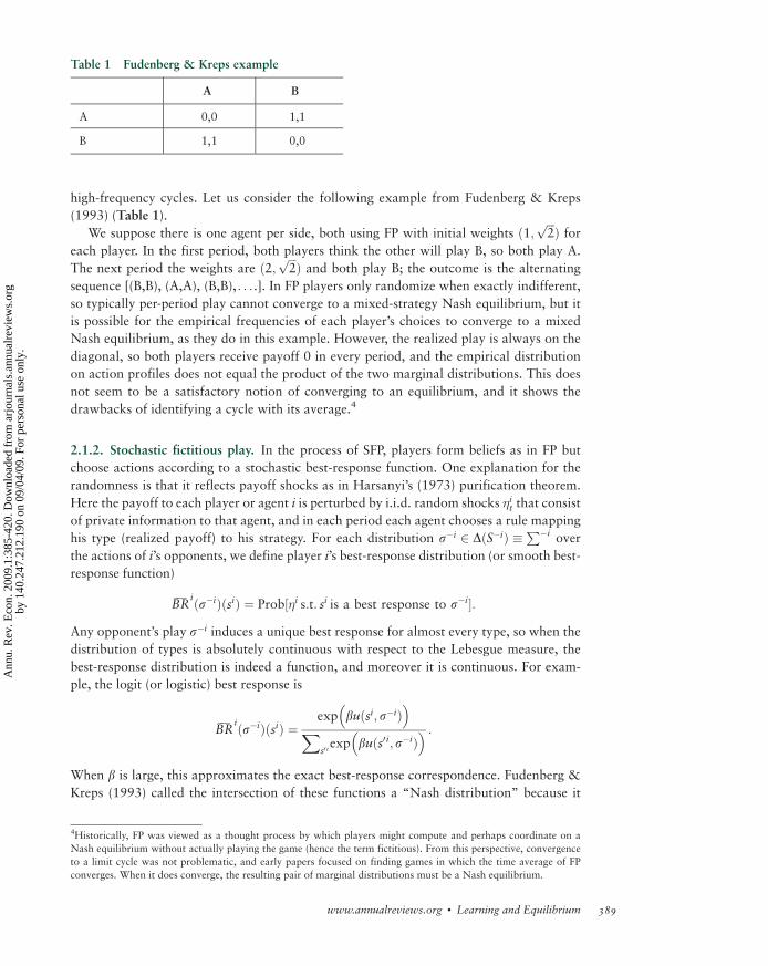
high-frequency cycles. Let us consider the following example from Fudenberg & Kreps
(1993) (Table 1).
We suppose there is one agent per side, both using FP with initial weights ð1; ffiffiffi2
p Þ foreach player. In the first period, both players think the other will play B, so both play A.
The next period the weights are ð2; ffiffiffi2
p Þ and both play B; the outcome is the alternating
sequence [(B,B), (A,A), (B,B), . . ..]. In FP players only randomize when exactly indifferent,
so typically per-period play cannot converge to a mixed-strategy Nash equilibrium, but it
is possible for the empirical frequencies of each player’s choices to converge to a mixed
Nash equilibrium, as they do in this example. However, the realized play is always on the
diagonal, so both players receive payoff 0 in every period, and the empirical distribution
on action profiles does not equal the product of the two marginal distributions. This does
not seem to be a satisfactory notion of converging to an equilibrium, and it shows the
drawbacks of identifying a cycle with its average.4
2.1.2. Stochastic fictitious play. In the process of SFP, players form beliefs as in FP but
choose actions according to a stochastic best-response function. One explanation for the
randomness is that it reflects payoff shocks as in Harsanyi’s (1973) purification theorem.
Here the payoff to each player or agent i is perturbed by i.i.d. random shocks �it that consist
of private information to that agent, and in each period each agent chooses a rule mapping
his type (realized payoff) to his strategy. For each distribution s�i 2 DðS�iÞ � P�i over
the actions of i’s opponents, we define player i’s best-response distribution (or smooth best-
response function)
���BR
iðs�iÞðsiÞ ¼ Prob½�i s:t: si is a best response to s�i�:Any opponent’s play s�i induces a unique best response for almost every type, so when the
distribution of types is absolutely continuous with respect to the Lebesgue measure, the
best-response distribution is indeed a function, and moreover it is continuous. For exam-
ple, the logit (or logistic) best response is
���BR
iðs�iÞðsiÞ ¼exp
�buðsi; s�iÞ
�X
s0 iexp
�buðs0i; s�iÞ
� :
When b is large, this approximates the exact best-response correspondence. Fudenberg &
Kreps (1993) called the intersection of these functions a “Nash distribution” because it
Table 1 Fudenberg & Kreps example
A B
A 0,0 1,1
B 1,1 0,0
4Historically, FP was viewed as a thought process by which players might compute and perhaps coordinate on a
Nash equilibrium without actually playing the game (hence the term fictitious). From this perspective, convergence
to a limit cycle was not problematic, and early papers focused on finding games in which the time average of FP
converges. When it does converge, the resulting pair of marginal distributions must be a Nash equilibrium.
www.annualreviews.org � Learning and Equilibrium 389
Ann
u. R
ev. E
con.
200
9.1:
385-
420.
Dow
nloa
ded
from
arj
ourn
als.
annu
alre
view
s.or
gby
140
.247
.212
.190
on
09/0
4/09
. For
per
sona
l use
onl
y.
corresponds to the Nash equilibrium of the static Bayesian game corresponding to the
payoff shocks; as b goes to infinity, the Nash distributions converge to the Nash equilibri-
um of the complete-information game.5
As compared with FP, SFP has several advantages: It allows a more satisfactory expla-
nation for convergence to mixed-strategy equilibria in FP-like models. For example, in the
matching-pennies game, the per-period play can actually converge to the mixed-strategy
equilibrium. In addition, SFP avoids the discontinuity inherent to standard FP, in which a
small change in the data can lead to an abrupt change in behavior. With SFP, if beliefs
converge, play does too. Finally, as we discuss in the next section, there is a (non-Bayesian)
sense in which stochastic rules perform better than deterministic ones: SFP is universally
consistent (or Hannan consistent) in the sense that its time-average payoff is at least as
good as maximizing against the time average of opponents’ play, which is not true for
exact FP.
For the analysis below, the source of the smooth best-response function is unimpor-
tant. It is convenient to think of it as having been derived from the maximization of a
perturbed deterministic payoff function that penalizes pure actions (as opposed to the
stochastic perturbations in the Harsanyi approach). Specifically, if vi is a smooth,
strictly differentiable, concave function on the interior of Si whose gradient becomes
infinite at the boundary, then arg maxsi uiðsi; s�iÞ þ b�1viðsiÞ is a smooth best-response
function that assigns positive probability to each of i’s pure strategies; the logit best
response corresponds to viðsiÞ ¼ Psi � siðsiÞlog siðsiÞ. It has been known for some
time that the logit model also arises from a random-payoff model in which payoffs
have the extreme-value distribution. Hofbauer & Sandholm (2002) extended this,
showing that if the smooth best responses are continuously differentiable and are
derived from a simplified Harsanyi model in which the random types have strictly
positive density everywhere, then they can be generated from an admissible determin-
istic perturbation.6
Now we consider systems of agents, all of whom use SFP. The technical insight here
is that the methods of stochastic approximation apply, so that the asymptotic properties
of these stochastic, discrete-time systems can be understood by reference to a limiting
continuous-time deterministic dynamical system. There are many versions of the stochas-
tic-approximation result in the literature. The following version from Benaım (1999)
is general enough for the current literature on SFP: We consider the discrete time process
on a nonempty convex subset X of Rm defined by the recursion xnþ1 � xn ¼½1=ðnþ 1Þ�½FðxnÞ þUn þ bn� and the corresponding continuous-time semiflow F induced
by the system of ordinary differential equations dxðtÞ=dt ¼ F½xðtÞ�, where the Un are
mean-zero, bounded-variance error terms, and bn ! 0. Under additional technical condi-
5Not all Nash equilibria can be approached in this way, as is the case with Nash equilibria in weakly dominated
strategies. Following McKelvey & Palfrey (1995), Nash distributions have become known in the experimental
literature as a quantal response equilibrium, and the logistic smoothed best response as the quantal best response.
6A key step is the observation that the derivative of the smooth best response is symmetric, and the off-diagonal
terms are negative: A higher payoff shock on i’s first pure strategy lowers the probability of every other pure
strategy. This means the smooth best-response function has a convex potential function: a function W (representing
maximized expected utility) such that the vector of choice probabilities is the gradient of the potential, analogous to
the indirect utility function in demand analysis. Hofbauer & Sandholm (2002) then show how to use the Legendre
transform of the potential function to back out the disturbance function. We note that the converse of the theorem is
not true: Some functions obtained by maximizing a deterministic perturbed payoff function cannot be obtained with
privately observed payoff shocks, and indeed Harsanyi had a counterexample.
390 Fudenberg � Levine
Ann
u. R
ev. E
con.
200
9.1:
385-
420.
Dow
nloa
ded
from
arj
ourn
als.
annu
alre
view
s.or
gby
140
.247
.212
.190
on
09/0
4/09
. For
per
sona
l use
onl
y.
tions,7 there is probability 1 that every o-limit8 of the discrete-time stochastic process lies
in a set that is internally chain-transitive for F.9 (It is important to note that the stochastic
terms do not need to be independent or even exchangeable.)
Benaım & Hirsch (1999) applied stochastic approximation to the analysis of SFP in
two-player games, with a single agent in the role of player 1 and a second single agent in
the role of player 2. The discrete-time system is then
where yi;n is player j’s beliefs about the play of player i, the Ui;n are the mean-zero error
terms, and the bi;n are asymptotically vanishing error terms that account for the difference
between player j’s beliefs and the empirical distribution of i’s play.10
They then used stochastic approximation to relate the asymptotic behavior of the
system to that of the deterministic continuous-time system
_y1 ¼ BR1ðy2Þ � y1; _y2 ¼ BR2ðy1Þ � y2 ðUnitaryÞ;where we call this system unitary to highlight the fact that there is a single agent in each
player role. Benaım & Hirsch also provided a similar result for games with more than two
players, still with one agent in each population. The rest points of this system are exactly
the equilibrium distributions. Thus stochastic approximation says roughly that SFP cannot
converge to a linearly unstable Nash distribution and that it has to converge to one of the
system’s internally chain-transitive sets.
Of course, this leaves open the issue of determining the chain-transitive sets for various
classes of games. Fudenberg & Kreps (1993) established global convergence to a Nash
distribution in 2 � 2 games with a unique mixed-strategy equilibrium. Benaım & Hirsch
(1999) provided a simpler proof of this, and established that SFP converges to a stable,
approximately pure Nash distribution in 2 � 2 games with two pure strategy equilibria;
they also showed that SFP does not converge in Jordan’s (1993) three-player matching-
pennies game. Hofbauer & Sandholm (2002) used the relationship between smooth best
responses and deterministic payoff perturbations to construct a Lyapunov function for SFP
in zero-sum games and potential games (Monderer & Shapley 1996) and hence proved
(under mild additional conditions) that SFP converges to a steady state of the continuous-
time system. Hofbauer & Sandholm derived similar results for a one-population version of
SFP, in which two agents per period are drawn to play a symmetric game, and the outcome
of their play is observed by all agents; this system has the advantage of providing an
explanation for the strategic myopia assumed in SFP.
Ellison & Fudenberg (2000) studied the unitary system described above in 3�3
games, in cases in which smoothing arises from a sequence of Harsanyi-like stochastic
perturbations, with the size of the perturbation going to zero. They found that there
7These technical conditions are the measurability of the stochastic terms, integrability of the semiflow, and pre-
compactness of the xn.
8The o-limit set of a sample path fyng is the set of long-run outcomes: y is in the o-limit set if there is an increasing
sequence of periods fnkg such that ynk ! y as nk ! 1.
9These are sets that are compact, invariant, and do not contain a proper attractor.
10Benaım and Hirsch (1999) simplified their analysis by ignoring the prior weights so that beliefs are identified with
the empirical distributions.
www.annualreviews.org � Learning and Equilibrium 391
Ann
u. R
ev. E
con.
200
9.1:
385-
420.
Dow
nloa
ded
from
arj
ourn
als.
annu
alre
view
s.or
gby
140
.247
.212
.190
on
09/0
4/09
. For
per
sona
l use
onl
y.
are many games in which the local stability of a purified version of the totally mixed
equilibrium depends on the specific distribution of the payoff perturbations, and there are
some games for which no purifying sequence is stable. Sandholm (2007) re-examined the
local stability of purified equilibria in this unitary system and gave general conditions for
the (local) stability and instability of equilibrium, demonstrating that there is always
at least one stable purification of any Nash equilibrium when a larger collection of purify-
ing sequences is allowed. Hofbauer & Hopkins (2005) proved the convergence of the
unitary system in all two-player games that can be rescaled to be zero sum and in two-
player games that can be rescaled to be partnerships. They also showed that isolated
interior equilibria of all generic symmetric games are linearly unstable for all small sym-
metric perturbations of the best-response correspondence, in which the term sym-
metric perturbation means that the two players have the same smoothed best-response
functions. This instability result applies in particular to symmetric versions of Shap-
ley’s (1964) famous example and to non-constant-sum variations of the game rock-
scissors-paper.11 The overall conclusion seems to be fairly optimistic about convergence
in some classes of games, whereas it is pessimistic in others. For the most part, the above
papers motivated the unitary system described above as a description of the long-
run outcome of SFP, but Ely & Sandholm (2005) showed that the unitary system also
described the evolution of the population aggregates in their model of Bayesian popula-
tion games.
Fudenberg & Takahashi (2009) studied heterogeneous versions of SFP, with many
agents in each player role, and each agent only observing the outcome of their own match.
The bulk of their analysis assumes that all agents in a given population have the same
smooth best-response function.12 In the case in which there are separate populations of
player 1’s and player 2’s, and all agents play every period, the standard results extend
without additional conditions. Intuitively, because all agents in population 1 are observing
draws at the same frequency from a common (possibly time-varying) distribution, they
will eventually have the same beliefs. Consequently, it seems natural that the set of
asymptotic outcomes should be the same as in a system with one agent per population.
Similar results were obtained in a model with personal clocks, in which a single pair of
agents is selected to play each day, with each pair having a possibly different probability of
being selected, provided that (a) the population is sufficiently large compared to the
Lipschitz constant of the best-response functions, and (b) the matching probabilities of
various agents are not too different. Under these conditions, although different agents
observe slightly different distributions, their play is sufficiently similar that their beliefs
are the same in the long run. Although this provides some support for results derived from
the unitary system above, the condition on the matching probabilities is fairly strong and
rules out some natural cases, such as interacting only with neighbors; the asymptotics of
SFP in these cases is an open question.
Benaım et al. (2007) extended stochastic-approximation analysis from SFP to weight-
ed stochastic FP, in which agents give geometrically less weight to older observations.
Roughly speaking, weighted smooth FP with weights converging to 1 gives the
11The constant-sum case is one of the nongeneric games in which the equilibrium is stable.
12The perturbations used to generate smoothed best responses may also be heterogeneous. Once this is allowed, the
beliefs of the different agents can remain slightly different, even in the limit, but a continuity argument shows that
this has little impact when the perturbations are small.
Local stability:
property of
converging to or
remaining near a set of
points when thesystem starts out
sufficiently close to
them
392 Fudenberg � Levine
Ann
u. R
ev. E
con.
200
9.1:
385-
420.
Dow
nloa
ded
from
arj
ourn
als.
annu
alre
view
s.or
gby
140
.247
.212
.190
on
09/0
4/09
. For
per
sona
l use
onl
y.
same trajectories and limit sets as SFP; the difference is in the speed of motion and,
hence, in whether the empirical distribution converges. They considered two related
models, both with a single population playing a symmetric game, unitary beliefs, and a
common smooth best-response function. In one model, there is a continuum population,
all agents are matched each period, and the aggregate outcome Xt is announced at
the end of period t. The aggregate common belief then evolves according to
xtþ1 ¼ ð1� gtÞxt þ gtXt, where gt is the step size. Because of the continuum of agents,
this is a deterministic system. In the second model, one pair of agents is drawn to play
each period, and a single player’s realized action is publicly announced. All players
update according to xtþ1 ¼ ð1� gtÞxt þ gtXt, where Xt is the action announced at peri-
od t. [Standard SFP has step size gt ¼ 1=ðt þ 1Þ; this is what makes the system slow
down and leads to stochastic-approximation results. It is also why play can cycle too
slowly for time averages to exist.]
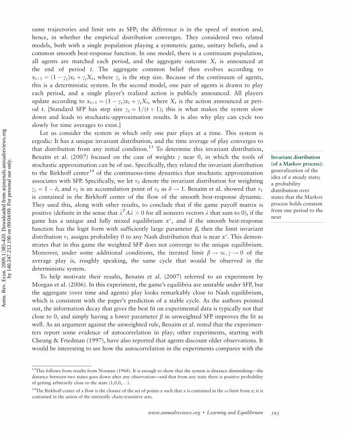
Let us consider the system in which only one pair plays at a time. This system is
ergodic: It has a unique invariant distribution, and the time average of play converges to
that distribution from any initial condition.13 To determine this invariant distribution,
Benaım et al. (2007) focused on the case of weights g near 0, in which the tools of
stochastic approximation can be of use. Specifically, they related the invariant distribution
to the Birkhoff center14 of the continuous-time dynamics that stochastic approximation
associates with SFP. Specifically, we let nd denote the invariant distribution for weighting
gt ¼ 1� d, and n1 is an accumulation point of nd as d ! 1. Benaım et al. showed that n1is contained in the Birkhoff center of the flow of the smooth best-response dynamic.
They used this, along with other results, to conclude that if the game payoff matrix is
positive (definite in the sense that lTAl > 0 for all nonzero vectors l that sum to 0), if the
game has a unique and fully mixed equilibrium x�, and if the smooth best-response
function has the logit form with sufficiently large parameter b, then the limit invariant
distribution n1 assigns probability 0 to any Nash distribution that is near x�. This demon-
strates that in this game the weighted SFP does not converge to the unique equilibrium.
Moreover, under some additional conditions, the iterated limit b ! 1; g ! 0 of the
average play is, roughly speaking, the same cycle that would be observed in the
deterministic system.
To help motivate their results, Benaım et al. (2007) referred to an experiment by
Morgan et al. (2006). In this experiment, the game’s equilibria are unstable under SFP, but
the aggregate (over time and agents) play looks remarkably close to Nash equilibrium,
which is consistent with the paper’s prediction of a stable cycle. As the authors pointed
out, the information decay that gives the best fit on experimental data is typically not that
close to 0, and simply having a lower parameter b in unweighted SFP improves the fit as
well. As an argument against the unweighted rule, Benaım et al. noted that the experimen-
ters report some evidence of autocorrelation in play; other experiments, starting with
Cheung & Friedman (1997), have also reported that agents discount older observations. It
would be interesting to see how the autocorrelation in the experiments compares with the
13This follows from results from Norman (1968). It is enough to show that the system is distance diminishing—the
distance between two states goes down after any observation—and that from any state there is positive probability
of getting arbitrarily close to the state (1,0,0,. . .).
14The Birkhoff center of a flow is the closure of the set of points x such that x is contained in the o-limit from x; it is
contained in the union of the internally chain-transitive sets.
Invariant distribution
(of a Markov process):
generalization of the
idea of a steady state;
a probabilitydistribution over
states that the Markov
process holds constant
from one period to thenext
www.annualreviews.org � Learning and Equilibrium 393
Ann
u. R
ev. E
con.
200
9.1:
385-
420.
Dow
nloa
ded
from
arj
ourn
als.
annu
alre
view
s.or
gby
140
.247
.212
.190
on
09/0
4/09
. For
per
sona
l use
onl
y.
autocorrelation predicted by weighed SFP, and whether the subjects were aware of these
cycles.
2.2. Asymptotic Performance and Global Convergence
SFP treats observations in all periods identically, so it implicitly assumes that the players
view the data as exchangeable. It turns out that SFP guarantees that players do at least as
well as maximizing against the time average of play, so when the environment is indeed
exchangeable, the learning rule performs well. However, SFP does not require that players
identify trends or cycles, which motivates the consideration of more sophisticated learning
rules that perform well in a wider range of settings. This in turn leads to the question of
how to assess the performance of various learning rules.
From the viewpoint of economic theory, it is tempting to focus on Bayesian learning
procedures, but these procedures do not have good properties against possibilities that
have zero prior probability (Freedman 1965). Unfortunately, any prior over infinite his-
tories must assign probability zero to very large collections of possibilities.15 Worse, in
interacting with equally sophisticated (or more sophisticated) players, the interaction
between the players may force the play of opponents to have characteristics that were a
priori thought to be impossible,16 which leads us to consider non-Bayesian optimality
conditions of various sorts.
Because FP and SFP only track frequencies (and not information relevant to identifying
cycles or other temporal patterns), there is no reason to expect them to do well, except
with respect to frequencies, so one relevant non-Bayesian criterion is to get (nearly) as
much utility as if the frequencies are known in advance, uniformly over all possible
probability laws over observations. If the time average of utility generated by the learning
rules attains this goal asymptotically, we say that it is universally consistent or Hannan
consistent. The existence of universally consistent learning rules was first proved by
Hannan (1957) and Blackwell (1956a). A variant of this result was rediscovered in the
computer science literature by Banos (1968) and Megiddo (1980), who showed that there
are rules that guarantee a long-run average payoff of at least the min-max. The existence
of universally consistent rules follows also from Foster & Vohra’s (1998) result on the
existence of universally calibrated rules, which we discuss below.
Universal consistency implicitly says that in the matching-pennies game, if the other
player plays heads in odd periods and tails in even periods, a good performance is winning
half the time, even though it would be possible to always win. This is reasonable, as it
would only make sense to adopt “always win” as the benchmark for learning rules that
have the ability to identify cycles.
To prove the existence of universally consistent rules, Blackwell (1956b) (discussed in
Luce & Raiffa 1957) used his concept of approachability (introduced in Blackwell 1956a).
15If each period has only two possible outcomes, the set of histories is the same as the set of binary numbers between
0 and 1. Let us consider on the unit interval the set consisting of a ball around each rational point, in which the
radius of the k-th ball is r=k2. This is big in the sense that it is open and dense, but when r is small, the set has a small
Lebesgue measure (see Stinchcombe 2005 for an analysis using more sophisticated topological definitions of what it
means for a set to be small).
16Kalai & Lehrer (1993) rule this out by an assumption that requires a fixed-point-like consistency in the players’
prior beliefs. Nachbar (1997) demonstrated that “a priori impossible” play is unavoidable when the priors are
required to be independent of the payoff functions in the game.
Universally consistent
rule: learning
procedure that obtainsthe same long-run
payoff as could be
obtained if thefrequency of
opponents’ choices
were known in
advance
394 Fudenberg � Levine
Ann
u. R
ev. E
con.
200
9.1:
385-
420.
Dow
nloa
ded
from
arj
ourn
als.
annu
alre
view
s.or
gby
140
.247
.212
.190
on
09/0
4/09
. For
per
sona
l use
onl
y.
Subsequently, Hart & Mas-Colell (2001) used approachability in a different way to
construct a family of universally consistent rules. Benaım et al. (2006) further refined this
approach, using stochastic-approximation results for differential inclusions. For SFP,
Fudenberg & Levine (1995) used a stochastic-approximation argument applied to the
difference between the realized payoff and the consistency benchmark, similar in spirit to
the original proof by Hannan; subsequently they used a calculation based on the assump-
tion that the smooth best-response functions are derived from maximizing a perturbed
deterministic payoff function and thus have symmetric cross partials (Fudenberg & Levine
1999).17
The Fudenberg & Kreps (1993) example shows that FP is not universally consistent.
However, Fudenberg & Levine (1995) and Monderer et al. (1997) demonstrated that
when FP fails to be consistent, it must result in the player employing the rule of frequently
switching back and forth between his strategies. In other words, the rule only fails to
perform well if the opponent plays so as to keep the player near indifferent. Moreover, it
is easy to show that no deterministic learning rule can be universally consistent, in the
sense of being consistent in all games against all possible opponents’ rules: For example, in
the matching-pennies game, given any deterministic rule, it is easy to construct an oppos-
ing rule that beats it in every period. This suggests that a possible fix would be to
randomize when nearly indifferent, and indeed Fudenberg & Levine (1995) showed that
SFP is universally consistent.
This universality property (called the worst-case analysis in computer science) has
proven important in the theory of learning, perhaps because it is fairly easy to achieve.
However, getting the frequencies asymptotically right is a weak criterion, as it allows a
player to ignore the existence of simple cycles, for example. Aoyagi (1996) studied an
extension of FP in which agents test the history for patterns, which are sequences of
outcomes. Agents first check for the pattern of length 1 corresponding to yesterday’s
outcome and count how often this outcome has occurred in the past. Then they look at
the pattern corresponding to the two previous outcomes and see how often it has oc-
curred, and so on. Player i recognizes a pattern p at history h if the number of its
occurrences exceeds an exogenous threshold that is assumed to depend only on the length
of p. If no pattern is recognized, beliefs are the empirical distribution. If one or more
patterns are detected, one picks one pattern (the rule for picking which one can be
arbitrary) and lets beliefs be a convex combination of the empirical distribution and the
empirical conditional distribution in periods following this pattern. Aoyagi shows that this
form of pattern detection has no impact on the long-run outcome of the system under
some strong conditions on the game being played.
Lambson & Probst (2004) considered learning rules that are a special case of those
presented by Aoyagi and derive a result for general games: If the two players use equal
pattern lengths and exact FP converges, then the empirical distribution of play converges
to the convex hull of the set of Nash equilibria. We expect that detecting longer patterns is
an advantage. Lambson & Probst do not have general theorems about this, but they have
an interesting example. In the matching-pennies game, there is a pair of rules in which one
player (e.g., player 1) has pattern length 0, the other (player 2) has pattern length 1, and
player 2 always plays a static best response to player 1’s anticipated action. We note that
17The Hofbauer & Sandholm (2002) result mentioned above showed that this same symmetry condition applies to
smooth best responses generated by stochastic payoff shocks.
www.annualreviews.org � Learning and Equilibrium 395
Ann
u. R
ev. E
con.
200
9.1:
385-
420.
Dow
nloa
ded
from
arj
ourn
als.
annu
alre
view
s.or
gby
140
.247
.212
.190
on
09/0
4/09
. For
per
sona
l use
onl
y.
this claim lets us choose the two rules together. We specify that player 2’s prior is that
player 1 will play T following the first time (H, T) occurs and H following the first time
(T, H) occurs. Let us suppose also that if players are indifferent, they play H, and that they
start out expecting their opponent to play H. Then the first period outcome is (H,T), the
next period is (T,H), the third period is (H,T) (because player 1 plays H when indifferent),
and so on.18
In addition, the basic model of universal consistency can be extended to account for
some conditional probabilities by directly estimating conditional probabilities using a sieve
as in Fudenberg & Levine (1999) or by the method of experts used in computer science.
This method, roughly speaking, takes a finite collection of different experts corresponding
to different dynamic models of how the data are generated, and shows that asymptotically
it is possible in the worst case to do as well as the best expert.19 That is, within the class of
dynamic models considered, there is no reason to do less well than the best.
2.2.1. Calibration. Although universal consistency seems to be an attractive property for
a learning rule, it is fairly weak. Foster & Vohra (1997) introduced learning rules derived
from calibrated forecasts. Calibrated forecasts can be explained in the setting of weather
forecasts: Let us suppose that a weather forecaster sometimes says there is a 25% chance
of rain, sometimes a 50% chance, and sometimes a 75% chance. Then looking over all her
past forecasts, if it actually rained 25% of the time on all the days she said 25% chance of
rain, it rained 50% of the time when she said 50%, and it rained 75% of the time when he
said 75%, we would say that she was well calibrated. As Dawid (1982) pointed out, no
rule whose forecasts are a deterministic function of the state can be calibrated in all
environments, for much the same reason that no deterministic behavior rule is universally
consistent in the matching-pennies game. For any deterministic forecast rule, we can find
at least one environment that beats it. However, just as with universal consistency, calibra-
tion can be achieved with randomization, as shown by Foster & Vohra (1998).
Calibration seems a desirable property for a forecaster to have, and there is some
evidence that weather forecasters are reasonably well calibrated (Murphy & Winkler
1977). However, there is also evidence that experimental subjects are not well calibrated
about their answers to trivia questions (such as, what is the area of Nigeria?) although the
interpretation and relevance of these experiments are under dispute (e.g., see Gigerenzer
et al. 1991).
In a game or decision problem, the question corresponding to calibration is, on all the
occasions in which a player took a particular action, how good a response was it? In other
words, choosing action A is a prediction that it is a best response. If we take the frequency
of opponents’ play on all those periods in which that prediction was made, we can
ask, was A actually a best response in those periods? Or, as demonstrated by Hart &
Mas-Colell (2000), we can measure this by regret: How much loss has the player suffered
in those periods by playing A rather than the actual best response to the frequency over
those periods? If the player is asymptotically calibrated in the sense that the time-average
18If we specify that player 2 plays H whenever there are no data for the relevant pattern (e.g., that the prior for this
pattern is that player 1 plays T), then player 2 only wins two-thirds of the time.
19This work was initiated by Vovk (1990) and is summarized, along wtih subsequent developments, by Fudenberg
& Levine (1998). There are also a few papers in computer science that analyze other models of cycle detection
combined with exact, as opposed to smooth, fictitious play.
396 Fudenberg � Levine
Ann
u. R
ev. E
con.
200
9.1:
385-
420.
Dow
nloa
ded
from
arj
ourn
als.
annu
alre
view
s.or
gby
140
.247
.212
.190
on
09/0
4/09
. For
per
sona
l use
onl
y.
regret for each action goes to zero (regardless of the opponents’ play), we say that the
player is universally calibrated. Foster & Vohra (1998) showed that there are learning
procedures that have this property, and proved that if all players follow such rules, the
time average of the frequency of play must converge to the set of correlated equilibria of
the game (Foster & Vohra 1997).
Because the algorithm originally used by Foster & Vohra involved a complicated
procedure of finding stochastic matrices and their eigenvectors, one might ask whether it
is a good approximation to assume that players follow universally calibrated rules. The
universal aspect of universal calibration makes it impossible to empirically verify without
knowing the actual rules that players use, but it is conceptually easy to tell whether
learning rules are calibrated along the path of play: If they are, the time average of joint
play converges to the set of correlated equilibria. If, conversely, some player is not cali-
brated along the path of play, he might notice that the environment is negatively correlated
with his play, which should lead him to second-guess his planned actions. For example, if
it never rains when the agent carries an umbrella, he might think along the following lines:
“I was going to carry an umbrella, so that means it will be sunny and I should not carry an
umbrella after all.” Just as with failures of stationarity, some forms of noncalibration are
more subtle and difficult to detect, but, even so, universally calibrated learning rules need
not be exceptionally complex.
We do not focus on the algorithm of Foster & Vohra. Subsequent research has greatly
expanded the set of rules known to be universally calibrated and greatly simplified the
algorithms and methods of proof. In particular, universally consistent learning rules may
be used to construct universally calibrated learning rules by solving a fixed-point problem,
which roughly corresponds to solving the fixed-point problem of second-guessing whether
to carry an umbrella. This fixed-point problem is a linear problem that is solved by
inverting a matrix, as shown by Fudenberg & Levine (1998); the bootstrapping approach
was subsequently generalized by Hart & Mas-Colell (2000).
Although inverting a matrix is conceptually simple, one may still wonder whether it is
simple enough for people to do in practice. We consider the related problem of arbitrage
pricing, which also involves inverting a matrix. Obviously, people tried to arbitrage before
there were computers or simple matrix-inversion routines. Whatever method they used
seems to have worked reasonably well because an examination of price data does not
reveal large arbitrage opportunities (e.g., see Black & Scholes 1972, Moore & Juh 2006).
Large Wall Street arbitrage firms do not invert matrices by the seat of their pants but by
explicit calculations on a computer, which may demonstrate that actual matrix inversion
works better.20
We should also point out the subtle distinction between calibration and universal
calibration. For example, Hart & Mas-Colell (2001) examined simple algorithms that
lead to calibrated learning, even though they are not universally calibrated. Formally, the
fixed-point problem that needs to be solved for universal calibration has the form
Rq ¼ RTq, where q are the probabilities of choosing different strategies, and R is a matrix
in which each row is the probability over actions derived by applying a universally
consistent procedure to each conditional history of a player’s own play. Let us suppose, in
20That people can implement sophisticated learning algorithms, both on their own and by using modern computers,
shows the limitations of conclusions based only on studies of simple learning tasks, including functional magnetic-
resonance-imaging scans of subjects doing simple learning.
Calibrated learning
procedure: learning
procedure such that in
the long run eachaction is a best
response to the
frequency distribution
of opponents’ choicesin all periods in which
that action was played
www.annualreviews.org � Learning and Equilibrium 397
Ann
u. R
ev. E
con.
200
9.1:
385-
420.
Dow
nloa
ded
from
arj
ourn
als.
annu
alre
view
s.or
gby
140
.247
.212
.190
on
09/0
4/09
. For
per
sona
l use
onl
y.
fact, the player played action a last period. We let m be a large number, and consider then
defining current probabilities by
qðbÞ ¼ ð1=mÞRða; bÞ1�
Xc6¼a
qðcÞb 6¼ ab ¼ a
:
�����
Although this rule is not universally calibrated, Hart & Mas-Colell (2000) showed that it
is calibrated provided everyone else uses similar rules. Cahn (2001) demonstrated that the
rule is also calibrated provided that everyone else uses rules that change actions at a
similar rate. Intuitively, if other players do not change their play quickly, the procedure
above implicitly inverts the matrix needed to solve Rq ¼ RTq.
2.2.2. Testing. One interpretation of calibration is that the learner has passed a test for
learning, namely getting the frequencies right asymptotically, even though the learner started
by knowing nothing. This has led to a literature that asks when and whether a person
ignorant of the true law-generating signals could fool a tester. Sandroni (2003) proposed
two properties for a test: It should declare pass/fail after a finite number of periods, and it
should pass the truth with high probability. If there is an algorithm that can pass the test with
high probability without knowing the truth, Sandroni says that it ignorantly passes the test.
He showed that for any set of tests that gives an answer in finite time and passes the truth
with high probability, there is an algorithm that can ignorantly pass the test.
Subsequent work has shown some limitations of this result. Dekel & Feinberg (2006)
and Olszewski & Sandroni (2006) relaxed the condition that the test yield a definite result
in finite time. They demonstrated that such a test can screen out ignorant algorithms, but
only by using counterfactual information. Fortnow & Vohra (2008) showed that an
ignorant algorithm that passes certain tests must necessarily be computationally complex,
and Al-Najjar & Weinstein (2007) demonstrated that it is much easier to distinguish
which of two learners is informed than to evaluate one learner in isolation. Feinberg &
Stewart (2007) considered the possibility of comparing many different experts, some real
and some false, and showed that only the true experts are guaranteed to pass the test
regardless of the actions of the other experts.
2.2.3. Convergence to Nash Equilibrium. There are two reasons we are interested in
convergence to Nash equilibrium. First, Nash equilibrium is widely used in game theory,
so it is important to know when learning rules do and do not lead to it. Second, Nash
equilibrium (in a strategic-form game) can be viewed as characterizing situations in which
no further learning is possible; conversely, when learning rules do not converge to Nash
equilibrium, some agent could gain by using a more sophisticated rule.
This question has been investigated by examining a class of learning rules to determine
whether Nash equilibrium is reached when all players employ learning rules in the class.
For example, we have seen that if all players employ universally calibrated learning rules,
then play converges to the set of correlated equilibrium. However, this means that players
may be correlating their play through the use of time as a correlating device, and why
should players not learn this? In particular, are there classes of learning rules that lead to
global convergence to a Nash equilibrium when employed by all players?
Preliminary results in this direction were negative. Learning rules are referred to as
uncoupled if the equation of motion for each player does not depend on the payoff
398 Fudenberg � Levine
Ann
u. R
ev. E
con.
200
9.1:
385-
420.
Dow
nloa
ded
from
arj
ourn
als.
annu
alre
view
s.or
gby
140
.247
.212
.190
on
09/0
4/09
. For
per
sona
l use
onl
y.
function of the other players. (It can of course depend on their actual play.) Hart & Mas-
Colell (2003) showed that uncoupled and stationary deterministic continuous-time adjust-
ment systems cannot be guaranteed to converge to equilibrium in a game; this result has
the flavor of Saari & Simon’s (1978) result that price dynamics uncoupled across markets
cannot converge to Walrasian equilibrium. Hart & Mas-Colell (2006) proved that conver-
gence to equilibrium cannot be guaranteed in stochastic discrete-time adjustment proce-
dures in the one-recall case in which the state of the system is the most recent profile of
play. They also refined Foster & Young’s past convergence result by showing that conver-
gence can be guaranteed in stochastic discrete-time systems in which the state corresponds
to play in the preceding two periods.
Despite this negative result, there may be uncoupled stochastic rules that converge
probabilistically to Nash equilibrium, as shown by a pair of papers by Foster & Young
Their first paper on this topic (Foster & Young 2003) showed the possibility of conver-
gence with uncoupled rules. However, the behavior prescribed by the rules strikes us as
artificial and poorly motivated. Their second paper (Foster & Young 2006) obtained the
same result with rules that are more plausible. (Further results can be found in Young
2008.)
In Foster & Young’s stochastic learning model, the learning procedure uses a status-
quo action that it periodically reevaluates. These reevaluations take place at infrequent
random times. During the evaluation period, some other action (randomly chosen with
probability uniformly bounded away from zero) is employed instead of the status-
quo action. That the times of reevaluation are random demonstrates a fair comparison
between the payoffs of the two actions. If the status quo is satisfactory in the sense that the
alternate action does not do much better, it is continued on the same basis (being reeval-
uated again). If it fails, then the learner concludes that the status-quo action was probably
not a good action. However, rather than adopting the alternative action, the learner goes
back to the drawing board and picks a new status-quo action at random.
We have seen above that if we drop the requirement of convergence in all environ-
ments, sensible procedures such as FP converge in many interesting environments (e.g., in
potential games). A useful counterpoint is the Shapley counterexample discussed above, in
which SFP fails to converge but instead approaches a limit cycle. Along this cycle, players
act as if the environment is constant, failing to anticipate their opponent’s play changing.
This raises the possibility of a more sophisticated learning rule in which players attempt to
forecast each other’s future moves. This type of model was first studied by Levine (1999),
who showed that players who were not myopic, but somewhat patient, would move away
from Nash equilibrium as they recognized the commitment value of their actions. Dynam-
ics in the purely myopic setting of attempting to forecast the opponent’s next play is
studied by Shamma & Arslan (2005).
To motivate Shamma & Arslan’s model, we consider the environment of smooth FP
with exponential weighting of past observations,21 which has the convenient property of
being time homogeneous and limits attention to the case of two players. We let l be the
exponential weight and ziðtÞ be the vector over actions of player i that takes on the value 1
for the action taken in period t and 0 otherwise. Then the empirical weight frequency of
player i0s play is siðtÞ ¼ ð1� lÞziðt � 1Þ þ lsiðt � 1Þ. In SFP, at time t player i plays a
smoothed best response bi½s�iðt � 1Þ� to this empirical frequency. However, s�iðt � 1Þ
21They use a more complicated derivation from ordinary FP.
www.annualreviews.org � Learning and Equilibrium 399
Ann
u. R
ev. E
con.
200
9.1:
385-
420.
Dow
nloa
ded
from
arj
ourn
als.
annu
alre
view
s.or
gby
140
.247
.212
.190
on
09/0
4/09
. For
per
sona
l use
onl
y.
measures what �i did in the past, not what she is doing right now. It is natural to
think, then, of extrapolating �i’s past play to get a better estimate of her current play.
Shamma & Arslan, motivated by the use of proportional derivative control to obtain
control functions with better stability properties, introduced an auxiliary variable r�i with
which to do this extrapolation. This auxiliary variable tracks s�i, so changes in the
auxiliary variable can be used to forecast changes in s�i. Specifically, let us suppose that
r�iðtÞ ¼ r�iðt � 1Þ þ l½s�iðt � 1Þ � r�iðt � 1Þ�; that is, r�i adjusts to reduce the distance to
s�i. The extrapolation procedure is then to forecast player �i’s play as
s�iðt � 1Þ þ g½r�iðtÞ � r�iðt � 1Þ�, the case g ¼ 0 corresponding to the exponentially
weighted FP, whereas g > 0 corresponds to giving some weight to the estimate rðtÞ of thederivative. This estimate is essentially the most recent increment in s�i when l is very
large; smaller values of l correspond to smoothing by considering past increments as well.
Motivated by stochastic approximation (which requires the exponential weighting in
beliefs be close to 1), Shamma & Arslan then studied the continuous-time analog of this
system. For the evolution of the state variable, _si ¼ f½biðs�i þ g_r�iÞ � si�, which comes
from taking the expected value of the adjustment equation for the weighted average,
where f is the exponential weight.22 The equation of motion for the auxiliary variable is
just _r�i ¼ lðs�i � r�iÞ.From the auxiliary equation, €r�i ¼ lð _s�i � _r�iÞ so that _r�i will be a good estimate of _s�i
if €r�i is small. When €r�i is small, Shamma & Arslan demonstrated that the system globally
converges to a Nash-equilibrium distribution. However, good known conditions on funda-
mentals that guarantee this result do not exist. In some cases of practical interest, however,
such as the Shapley example, simulations show that the system does converge.
2.3. Reinforcement Learning, Aspirations, and Imitation
Now we consider the nonequilibrium dynamics of various forms of boundedly rational
learning, starting with models in which players act as if they do not know the payoff
matrix23 and do not observe (or do not respond to) opponent’s actions. We then move on
to models that assume players do respond to data such as the relative frequency and
payoffs of the strategies that are currently in use.
Reinforcement learning has a long history in the psychology literature. Perhaps the
simplest model of reinforcement learning is the cumulative proportional reinforcement
(CPR) model studied by Laslier et al. (2001). In this process, utilities are normalized to
be positive, and the agent starts out with initial weights CUkð1Þ to each action k. Thereaf-
ter, the process updates the score (also called a propensity) of the action that was played
by its realized payoff and does not update the scores of other actions. The probability
of action k at time t is then CUkðtÞ=P
jCUjðtÞ. We note that the step size of this process,
the amount that the score is updated, is stochastic and depends on the history to date,
22Shamma & Arslan (2005) chose the units of time so that f ¼ 1. In these time units, it takes one unit of time to
reach the best response, so that choosing g ¼ 1 means that the extrapolation attempts to guess what other players
will be doing at the time full adjustment to the best response takes place. Shamma & Arslan give a special
interpretation to this case, which they refer to as “system inversion.”
23This behavior might arise either because players do not have this information or because they ignore it owing to
cognitive limitations. However, there is evidence that providing information on opponents’ actions does change the
way players adapt their play (see Weber 2003). Borgers et al. (2004) characterized monotone learning rules for
settings in which players observe only their own payoff.
400 Fudenberg � Levine
Ann
u. R
ev. E
con.
200
9.1:
385-
420.
Dow
nloa
ded
from
arj
ourn
als.
annu
alre
view
s.or
gby
140
.247
.212
.190
on
09/0
4/09
. For
per
sona
l use
onl
y.
in contrast to the 1=t increment in beliefs for a Bayesian learner in a stationary
environment.24
With this rule, every action is played infinitely often: The cumulative score of action k
is at least its initial value, and the sum of the cumulative payoffs at time t is at most the
initial sum plus t times the maximum payoff. Thus the probability of action k at time t is
at least a=ðbþ ctÞ for some positive constants a, b, and c, so the probability of never
playing k after time t is bounded by the productQ1
t¼t½1� a=ðbþ ctÞ� ¼ 0.
To analyze the process further, Laslier et al. used results on urn models: The state space
is the number of balls of each type, and each period one ball is added, so that the step size
is 1=t. Here the balls correspond to the possible action profiles ða1; a2Þ, and the state space
has dimension # A1�# A2 equal to the number of distinct action profiles. The number of
occurrences of a given joint outcome can increase by at most rate 1=t, and the number of
times that each outcome has occurred is a sufficient statistic for the realized payoffs and
the associated cumulative utility. One can then use stochastic-approximation techniques to
derive the associated ordinary differential equation _x ¼ �xþ rðxÞ, where x is the fraction
of occurrences of each type, and r is the probability of each profile as a function of the
current state.
Laslier et al. showed that when player 2 is an exogenous fixed distribution played by
nature, the solution to this equation converges to the set of maximizing actions from any
interior point, and, moreover, that the stochastic discrete-time CPR model does the same
thing. Intuitively, the system cannot lock on to the wrong action because every action is
played infinitely often (so that players can learn the value of each action) and the step size
converges to 0. Laslier et al. also analyzed systems with two agents, each using CPR (and
therefore acting as if they were facing a sequence of randomly drawn opponents). Some of
their proofs were based on incorrect applications of results on stochastic approximation
due to problems on the boundary of the simplex; Beggs (2005) and Hopkins & Posch
(2005) provided the necessary additional arguments, showing that even in the case of
boundary rest points, reinforcement learning does not converge to equilibria that are
unstable under the replicator dynamic and, in particular, cannot converge to non-Nash
states. Beggs showed that the reinforcement model converges to equilibrium in constant-
sum 2 � 2 games with a unique equilibrium, and Hopkins & Posch demonstrated conver-
gence to a pure equilibrium in rescaled partnership games. Because generically every 2 � 2
game is either a rescaled partnership game or a rescaled constant-sum game, what these
results leave open is the question of convergence in games that are rescaled constant sum
but not constant sum without the rescaling; work in progress by Hofbauer establishes that
reinforcement learning does converge in all 2 � 2 games.
Hopkins (2002) studied several perturbed versions of CPR with slightly modified
updating rules. In one version, the update rule is the same as CPR except that each period,
the score of every action is updated by an additional small amount l. Using stochastic
approximation, he related the local stability properties of this process to that of a per-
turbed replicator dynamic. He showed (roughly speaking) that if a completely mixed
equilibrium is locally stable for all smooth best-response dynamics, it is locally stable for
the perturbed replicator, and if an equilibrium is unstable for all smooth best-response
24Erev & Roth (1998) studied a perturbed version of this model in which every action receives a small positive
reinforcement in every period; Hopkins (2002) investigated a normalized version of this process in which the step
size is deterministic and of order 1/t.
www.annualreviews.org � Learning and Equilibrium 401
Ann
u. R
ev. E
con.
200
9.1:
385-
420.
Dow
nloa
ded
from
arj
ourn
als.
annu
alre
view
s.or
gby
140
.247
.212
.190
on
09/0
4/09
. For
per
sona
l use
onl
y.
dynamics, it is unstable for the perturbed replicator.25 He also obtained a global conver-
gence result for a normalized version of perturbed CPR in which the step size per period is
1=t, independent of the history.
Borgers & Sarin (1997) analyzed a related (unperturbed) reinforcement model, in
which the amount of reinforcement does not slow down over time but is instead a fraction
g, so that, in a steady-state environment, the cumulative utility of every action that is
played infinitely often converges to its expected value. Because the system does not slow
down over time, the fact that each action is played infinitely often does not imply that the
agent learns the right choice in a stationary environment, and indeed the system has
positive probability of converging to a state in which the wrong choice is made in every
period. At a technical level, stochastic-approximation results for systems with decreasing
steps do not apply to systems with a constant step size. Instead, Borgers & Sarin looked at
the limit of the process as the adjustment speed g goes to 0, and show that over finite time
horizons, the trajectories of the process converge to that of its mean field, which is the
replicator dynamic. (The asymptotics, however, are different: For example, in the matching-
pennies game, the reinforcement model will eventually be absorbed at a pure strategy
profile, whereas the replicator dynamic will not.) Borgers & Sarin (2000) extended this
model to allow the amount of reinforcement to depend on the agent’s aspiration level. In
some cases, the system does better with an aspiration level than in the base Borgers &
Sarin (1997) model, but aspiration levels can also lead to suboptimal probability-matching
outcomes.26
It is worth mentioning that an inability to observe opponents’ actions does not make it
impossible to implement SFP, or related methods, such as universally calibrated algo-
rithms. In particular, in SFP the utility of different alternatives is what matters. For
it is not important that the player observes s�i; he merely needs to see uðsi; s�iÞ, and there
are a variety of ways to use historical data on the player’s own payoffs to infer this.27
Moreover, we conjecture that the asymptotic behavior of a system in which agents learn in
this way will be the same as with SFP, although the relative probabilities of the various
attractors may change, and the speed of convergence will be slower.
Reinforcement learning requires only that the agent observe his own realized payoffs.
Several papers argue that agents can access the actions and perhaps the payoffs of other
members of the population, and thus can imitate the actions of those they observe.
Bjornerstedt & Weibull (1996) studied a deterministic, continuum-population model, in
which agents receive noisy statistical information about the payoff of other strategies and
switch to the strategy that appears to be doing the best. Binmore & Samuelson (1997)
studied a model of imitation with fixed aspirations in a large finite population playing a
25As mentioned in Section 2.1, two small perturbations of the same best-response function can have differing
implications for local stability.
26At one time psychologists believed that probability matching was a good description of human behavior, but
subsequent research showed that behavior moves away from probability matching if agents are offered monetary
rewards or simply given enough repetitions of the choice (Lee 1971).
27See Fudenberg & Levine (1998) and Hart & Mas-Colell (2001).
402 Fudenberg � Levine
Ann
u. R
ev. E
con.
200
9.1:
385-
420.
Dow
nloa
ded
from
arj
ourn
als.
annu
alre
view
s.or
gby
140
.247
.212
.190
on
09/0
4/09
. For
per
sona
l use
onl
y.
2 � 2 game.28 In the unperturbed version of the model, in each period, one agent receives
a learn draw and compares the payoff of his current strategy to the sum of a fixed
aspiration level and an i.i.d. noise term. (The agent plays an infinite number of rounds
between each learn draw so that this payoff corresponds to the strategy’s current expected
value.) If the payoff is above the target level, the agent sticks with his current strategy;
otherwise he imitates a randomly chosen individual. In the perturbed process, the agent
mutates to the other strategy with some fixed small probability l. Binmore & Samuelson
characterized the iterated limit of the invariant distribution of the perturbed process as the
population size going to infinity first and then the mutation rate shrinking to 0. In a
coordination game, this limit will always select one of the two pure-strategy equilibria,
but the risk-dominant equilibrium need not be selected because the selection procedure
reflects not only the size of the basins of attraction of the two equilibria, but also the
strength of the learning flow.29
A similar finding arises in the study of the frequency-dependent Moran process
(Nowak et al. 2004), which represents a sort of imitation of successful strategies combined
with the imitation of popular ones: When an agent changes his strategy, he picks a new
one based on the product of the strategy’s current payoff and its share of the population,
so if all strategies have the same current payoff, the probabilities of adoption exactly equal
the population shares, whereas if one strategy has a much higher payoff, its probability of
being chosen can be close to one. In the absence of mutations or other perturbations,
Binmore & Samuelson’s (1997) and Nowak et al.’s (2004) models both have the property
that every homogeneous state in which all agents play the same strategy is absorbing,
whereas every state in which two or more strategies are played is transient. Fudenberg &
Imhof (2006) gave a general algorithm for computing the limit invariant distribution in
these sorts of models for a fixed population size as the perturbation goes to 0 and applied
it to 3 � 3 coordination games and to Nowak et al.’s model. Benaım & Weibull (2003)
provided mean field results for the large-population limit of a more general class of
systems, in which the state corresponds to a mixed-strategy profile, only one agent
changes play per period, and the period length goes to 0 as the population goes to infinity.
Karandikar et al. (1998), Posch & Sigmund (1999), and Cho & Matsui (2005) analyzed
endogenous aspirations and inertia in two-action games. In their models, a fixed pair of
agents play each other repeatedly; the agents tend to play the action they played in the
previous period unless their realized payoff is less than their aspiration level, where the
aspiration level is the average of the agent’s realized payoffs.30 In Posch & Sigmund’s model,
the behavior rule is simple: If the payoff is at least the aspiration level, then a player should
play the same action with probability 1� e and switch with probability e. Symmetrically, if
the realized payoff is less than the aspiration level, then a player should switch with
probability 1� e and play the same action with probability e. In Krandikar et al.’s model,
the agent never switches if his realized payoff is at least the aspiration level; as the payoff
drops below the aspiration level, the probability of switching rises continuously to an
28Fudenberg & Imhof (2008) generalized their assumptions and extended the analysis to games with an arbitrary
finite number of actions.
29See Fudenberg & Harris (1992) for a discussion of the relative importance of the size of the basin and the cost of
“swimming against the flow.”
30Posch & Sigmund (1999) also analyzed a variant in which the aspiration level is yesterday’s payoff, as opposed to
the long-run average. Karandikar et al. (1998) focused on an extension of the model in which aspirations are
updated with noise.
www.annualreviews.org � Learning and Equilibrium 403
Ann
u. R
ev. E
con.
200
9.1:
385-
420.
Dow
nloa
ded
from
arj
ourn
als.
annu
alre
view
s.or
gby
140
.247
.212
.190
on
09/0
4/09
. For
per
sona
l use
onl
y.
upper bound p. Cho & Matsui also considered a smooth increasing switching function; in
contrast to Krandikar et al., they assume that there is a strictly positive probability of
switching if the payoff is in the neighborhood of the current aspiration level.
The key aspect of these models is that the aspiration levels eventually move much more
slowly than behavior because they update at a rate of 1=t. This allows Cho & Matsui to
apply stochastic-approximation techniques and relate the asymptotic behavior of the
system to that of the system _a ¼ ua � a, where a is the vector of aspiration levels, and uais the vector of average payoffs induced by the current aspiration level. (This vector is
unique because each given aspiration level corresponds to an irreducible Markov matrix
on actions.31) Cho & Matsui concluded that their model leads to coordination on the
Pareto-efficient equilibrium in a symmetric coordination game, and that play can converge
to always cooperate in the prisoner’s dilemma, provided that the gain from cheating is
sufficiently small compared to the loss incurred when the other player cheats. Krandikar
et al. obtained a similar result, except that it holds regardless of the gain to cheating, the
difference being that in their model agents who are satisfied stick with their current action
with probability 1.
In these models, players do not explicitly take into account that they are in a repeated
interaction, but cooperation nonetheless occurs.32 It is at least as interesting to model
repeated interactions when players explicitly respond to their opponent’s play, but the
strategy space in a repeated game is large, so analyses of learning dynamics have typically
either restricted attention to a small subset of the possible repeated game strategies or
analyzed related games in which the strategy space is in fact small. The first approach has
a long tradition in evolutionary biology, dating back to the work of Axelrod & Hamilton
(1981). Nowak et al. (2004) and Imhof et al. (2005) adopted it in their applications of the
Moran process to the repeated prisoner’s dilemma: Nowak et al. (2004) consider only the
two strategies “always defect” and “tit for tat,” and show that tit for tat is selected,
essentially because its basin becomes vanishingly small when the game is played a large
number of rounds. Imhof et al. (2005) add the strategy “always C,” which is assumed to
have a small complexity-cost advantage over tit for tat, resulting in cycles that spend most
of the time near “all tit for tat” if the population and the number of rounds are large.33
Jehiel (1999) considered a different sort of simplification: He supposed that players only
care about payoffs for the next k periods, and their opponent’s play only depends on the
outcomes in the past m periods.
Instead of imposing restrictions on the strategy space or beliefs, one can consider an
overlapping-generations framework in which players play just once, as in the gift-giving
game, in which young people may give a gift to an old person. Payoffs are such that it is
preferable to give a gift when young and receive one when old than to neither give nor
receive a gift. This type of setting was originally studied without learning by Kandori
(1992) who allowed information systems to explicitly carry signals about past play and
proved a folk theorem for a more general class of overlapping-generations games. Johnson
31According to Posch & Sigmund (1999), behavior is not a continuous function of the state. They do use simula-
tions to support the use of a similar equation, however.
32It is often possible to do well by being less than fully rational. This is especially important in situations in which
precommitment is an issue: Here it is advantageous for a player’s opponents to think she is irrationally committed.
An interesting example of such a learning rule and a typical result can be found in Acemoglu & Yildiz (2001).
33The result requires that the number of rounds is large given the population size.
404 Fudenberg � Levine
Ann
u. R
ev. E
con.
200
9.1:
385-
420.
Dow
nloa
ded
from
arj
ourn
als.
annu
alre
view
s.or
gby
140
.247
.212
.190
on
09/0
4/09
. For
per
sona
l use
onl
y.
et al. (2001) showed that a simple red/green two-signal information system can be used to
sustain cooperation, and this emerges as the limit of the invariant distribution under the
myopic best-response dynamic with mutations. Nowak & Sigmund (1998a,b) offered an
interpretation of Kandori’s information systems as a public image and used simulations of
a discrete-time replicator process to argue that play converges to a cooperative outcome.
Levine & Pesendorfer (2007) studied equilibrium selection in a related game under the
relative best-reply dynamic, in which players select the best reply to the current state
among the strategies that are currently active. To make the process ergodic, they assumed
that there are small perturbations corresponding both to imitation (copy a randomly
chosen agent) and mutation, with imitation much more likely than mutation. Levine &
Pesendorfer then analyzed the limiting invariant distribution in games in which players
simultaneously receive signals of each other’s intentions, use strategies that simultaneously
indicate intention, and respond to signals about the other player’s intention. These games
always have trivial equilibria in which the signals are ignored. Depending on the strength
of the signal, there can be more cooperative equilibria. For example, if players receive a
perfect indication that their opponent is using the same strategy as they are, then the
strategy of maximizing joint utility when the opponent is the same (but min-maxing
the difference in utilities when the opponent is different) is an equilibrium. Moreover,
Levine & Pesendorfer demonstrated that this equilibrium is selected in the limit of small
perturbations.
3. LEARNING IN EXTENSIVE-FORM GAMES
3.1. Incorrect Beliefs About Off-Path Play
In extensive-form games, it seems natural to assume that players observe at most which
terminal nodes are reached, so that they do not observe how their opponents would have
played at information sets that were not reached. This can allow incorrect beliefs about
off-path play to persist unless, for some reason, players obtain enough observations of off-
path play. This subsection reviews work on the baseline case in which players do observe
which terminal node is reached each time the game is played. The next subsection dis-
cusses extensions to more general information structures.
The possibility that incorrect beliefs can persist raises three questions: (a) What sorts of
long-run outcomes can occur when off-path beliefs are wrong? (b) How much off-path
play must occur to ensure that any long-run outcome is a Nash equilibrium or sequential
equilibrium? (c) How much off-path play will in fact occur under various models of
learning?
The set of outcomes that can persist in the absence of information about off-path play
is characterized by the notion of self-confirming equilibrium (SCE), of which there are
several versions. The most straightforward to define is that of unitary SCE, where the term
unitary emphasizes that there is a single belief for each player role. Unitary SCE requires
that for each player role i in the game, there are beliefs mi over opponents’ play (ordinarily
the space of their behavior strategies) that satisfy two basic criteria. First, players should
optimize relative to their beliefs. Second, beliefs should be correct at those information sets
on the game tree that are reached with positive probability. In other words, the beliefs
must assign probability 1 to the set of opponent behavior strategies that are consistent
with actual play at those information sets. Even this version of SCE allows outcomes that
Self-confirming
equilibrium (SCE):
strategy profile inwhich each player’s
action is a best
response to their
beliefs aboutopponents’ play, and
each player’s beliefs
are correct along theequilibrium path
www.annualreviews.org � Learning and Equilibrium 405
Ann
u. R
ev. E
con.
200
9.1:
385-
420.
Dow
nloa
ded
from
arj
ourn
als.
annu
alre
view
s.or
gby
140
.247
.212
.190
on
09/0
4/09
. For
per
sona
l use
onl
y.
are not Nash equilibria, as shown by Fudenberg & Kreps (1995), but it is outcome-
equivalent to Nash equilibrium in two-player games (Battigalli 1997, Fudenberg & Kreps
1995).34 The related concept of heterogeneous SCE applies when there is a population of
agents in each player role, so that different agents in the same player role can have
different beliefs. Here the beliefs of each agent must be consistent with what the agent
observes given its own choice of pure strategy, and different agents in the same player role
can have different beliefs provided that their actions lead them to observe different parts of
the game tree. Every unitary SCE is a heterogeneous SCE, but heterogeneous SCE permits
still more departures from Nash equilibrium outcomes, and these additional departures
seem to occur in experimental play of extensive-form games (Fudenberg & Levine 1997).
Although even unitary SCE is less restrictive than Nash equilibrium, it is by no means
vacuous. For example, Fudenberg & Levine (2005) showed that SCE is enough for the no-
trade theorem. Basically, if players make a purely speculative trade, some of them have to
lose, and they will notice this.
We turn now to the question, when is there enough experimentation to lead to a
stronger notion of equilibrium than SCE? Fudenberg & Kreps (1994) demonstrated that
non-Nash outcomes cannot persist if every action is played infinitely often at every infor-
mation set on the path of play, and observed that refinements such as sequential equilibri-
um additionally require that every action is played infinitely often at other information
sets as well. If behavior rules satisfy their modified minimal experience-time condition,
then actions are indeed played infinitely often on the path of play, and, moreover, every
action is played infinitely often in games of perfect information. For this reason, the only
stable outcomes in such games are the backward-induction solutions. However, they point
out that the modified minimal experience time condition requires more experimentation
than may be plausible, as it is not clear that players at seldomly reached information sets
will choose to do that much experimentation. This is related to the fact that, if each player
experiments at rate 1/t in period t, then players on the path of play experiment infinitely
often (becauseP1
t¼11=t ¼ 1), whereas players who are only reached when others experi-
ment will experiment a finite number of times (becauseP1
t¼11=t2 6¼ 1). Fudenberg &
Levine (1993b) examined endogenous experimentation and derived experimentation rates
from the hypothesis of expected-utility maximization, showing that there is enough exper-
imentation to rule out non-Nash outcomes when the discount factor is close enough to 1,
but they did not address the question of whether there will be enough experimentation to
rule out outcomes that are not subgame perfect.
Noldeke & Samuelson (1993) considered a large-population model of learning in
which experiments occur when the players mutate and change their beliefs and thus their
actions. Each period, all agents are matched to play the game. At the end of the period,
most players do not update their beliefs at all, but with some fixed probability a player
receives a learn draw, observes the terminal nodes that were reached in all of the games
that were played this period, and changes her beliefs about play at all reached information
sets to match the frequencies in her observation. Thus a mutation in the beliefs and play of
one agent can eventually lead all of them to learn from the mutating agent’s experiment. In
34More generally, unitary SCE with independent beliefs is outcome-equivalent to Nash equilibria in games with
observed deviators. Kamada (2008) fixed an error in the original Fudenberg & Levine (1993a) proof of this, which
relied on the claim that consistent unitary, independent SCE is outcome-equivalent to Nash equilibria. The defini-
tion given of consistency was too weak for this to be true, and Kamada give the appropriate definition.
Experimentation: play
of an action that is nota best response to
current beliefs to see if
those beliefs are
inaccurate
406 Fudenberg � Levine
Ann
u. R
ev. E
con.
200
9.1:
385-
420.
Dow
nloa
ded
from
arj
ourn
als.
annu
alre
view
s.or
gby
140
.247
.212
.190
on
09/0
4/09
. For
per
sona
l use
onl
y.
games of perfect information, this leads to a refinement of SCE, and, in some special cases,
such as when each player moves at most once on any path of play, it leads to subgame
perfection.
Dubey & Haimanko (2004) studied a similar model of learning in a game of perfect
information, in which agents play best responses to their beliefs, and beliefs are updated to
be consistent with observed data; the model is quite flexible in its interpretation, as it
allows players to consider only the most recent observation or older data as well. The
system converges to a (unitary) SCE with independent beliefs; because this is a game with
identified deviators, the steady state is thus outcome equivalent to a Nash equilibrium.
The belief-based models mentioned above place no constraints on the players’ beliefs
other than consistency with observed data and, in particular, are agnostic about what
prior information any player might have about the payoff functions of the others. Rubin-
stein & Wolinksy (1994) and Dekel et al. (1999) added the restriction that players do
know the payoff functions of the others, leading to the concepts of rationalizable conjec-
tural equilibrium and rationalizable self-confirming equilibrium (RSCE). To see the differ-
ence that this makes, we consider Dekel et al.’s variation on the game Fudenberg & Kreps
(1995) used to show the nonequivalence of SCE and unitary SCE with independent beliefs
(Figure 1).
Here if x and y have the same sign, then player 3 has a conditionally dominant strategy,
so if players 1 and 2 assign high probability to a neighborhood of player 30s true payoffs,then they must have similar beliefs about his play. In this case, (A,a) is not the outcome of
any RSCE. However, if x and y have opposite signs, then even common knowledge
of player 30s payoff function does not imply common beliefs about his play, and RSCE
allows (A,a).35 Another variation on this theme is Esponda’s (2008) SCE-motivated
robustness notion. He allowed players to be uncertain about hierarchies of beliefs, but
these hierarchies of beliefs are required to be consistent with players’ knowledge of
equilibrium play. Rationalizability, Nash equilibrium, and SCE are special cases. Despite
1 2
3
A
D d
(1,1,1)
(3,0,0) (0,3,x) (3,0,0) (0,3,y)
L RL
R
a
R
Figure 1
Dekel et al.’s (1999) variation on the game Fudenberg & Kreps (1995) used to show the nonequiva-
lence of self-confirming equilibrium and unitary self-confirming equilibrium with independent beliefs.
35Dekel et al. (1999) only defined RSCE for the unitary case; the appropriate heterogeneous definition, and its
consequences, is still unresolved.
www.annualreviews.org � Learning and Equilibrium 407
Ann
u. R
ev. E
con.
200
9.1:
385-
420.
Dow
nloa
ded
from
arj
ourn
als.
annu
alre
view
s.or
gby
140
.247
.212
.190
on
09/0
4/09
. For
per
sona
l use
onl
y.
the broad range of possibilities allowed, the solution may be characterized by an iterative
elimination procedure.
3.2. More General Information Structures
SCE is based on the idea that players should have correct beliefs about probability dis-
tributions that they observe sufficiently often, so that the specification of the observation
technology is essential. The original definition of SCE assumes that players observe the
terminal node that is reached, but in some settings it is natural to assume that they observe
less than this. For example, in a sealed-bid auction, players might only observe the
winning bid and the identity of the winning bidder, but observe neither the losing bids
nor the types of the other players. In the setting of a static Bayesian game, Dekel et al.
(2004) extended the definition of SCE to allow for these sorts of coarser maps from
outcomes of the game to observations. If players do observe the outcome of each round
of play (i.e., both the actions taken and the realization of nature’s move), the set of SCE is
the same as the set of Nash equilibria with a common prior. Dekel et al. pointed out that
the same conclusion applies if players observe the actions played and there are private
values, so that each player’s private information relates only to their own payoff. When
players do not observe the actions played, or there are not private values, the set of SCE
can include non-Nash outcomes. The authors argued that Nash equilibrium without a
common prior is difficult to justify as the long-run result of a learning process because it
takes special assumptions for the set of such equilibria to coincide with the set of steady
states that could arise from learning. Intuitively, Nash equilibrium requires that players
have correct beliefs about the strategies their opponents use to map their types to their
actions, and for repeated observations to lead players to learn the distribution of oppo-
nents’ strategies, the signals observed at the end of each round of play must be sufficiently
informative. Such information will tend to lead players to also have correct and hence
identical beliefs about the distribution of nature’s moves.
Although SCE assumes that the players’ inferences are consistent with their observa-
tions, a related strand of this literature assumes that players make systematic mistakes in
inference. The leading example here is Jehiel’s (2005) notion of analogy-based expectation
equilibrium (ABEE), in which players group the opponents’ decision nodes into analogy
classes, with the player believing that play at each node in a given class is identical. Given
this, the player’s beliefs must then correspond to the actual average of play across the
nodes in the analogy class.
For example, let us consider a game of perfect information, in which nature moves
first, choosing state A with two-thirds probability or state B with one-third probability,
player 1 moves second, choosing either action A1 or action B1, with player 2 moving
last, again choosing either action A2 or action B2. We suppose, for illustrative purposes,
that player 2 is a dummy receiving a zero payoff no matter what, and that player
2 chooses A in state A and B in state B regardless of player 1’s actions. Player 1 gets
one if his action matches that of player 2, and zero if not. Then in state A, player 1
should play A1, and in state B player 1 should play B1. However, if player 1 views all
nodes of player 2 following a given move as belonging to an analogy class, then he
believes that player 2 will play A2 two-thirds of the time, regardless of the state, so
player 1 plays A1 regardless of the state. If player 1 observes and remembers the
outcome of each game, then as he learns that player 2 plays A2 two-thirds of the time,
ABEE: analogy-based
expectationequilibrium
408 Fudenberg � Levine
Ann
u. R
ev. E
con.
200
9.1:
385-
420.
Dow
nloa
ded
from
arj
ourn
als.
annu
alre
view
s.or
gby
140
.247
.212
.190
on
09/0
4/09
. For
per
sona
l use
onl
y.
he also gets evidence that player 2’s play is correlated with the state. Thus if he is a
rational Bayesian and assigns positive probability to player 2 observing the state, he
should eventually learn that this is the case. Conversely, even a rational player 1 could
maintain the belief that player 2’s play is independent of the state provided that he has a
doctrinaire prior that assigns probability 1 to this independence. Such doctrinaire priors
may seem unreasonable, but they are an approximation of circumstances in which
player 1 has a very strong prior conviction that player 2’s play is independent of the
state. In this case it will take a very long time to learn that this is not true.36
An alternative explanation for analogy-based reasoning is that players are boundedly
rational, so they are unable to remember all that they have observed, perhaps because at
an earlier stage they chose not to expend the resources required for a better memory. In
our example, this would correspond to player 1 being able only to remember the fraction
of time that player 2 played A2 and not the correlation of this play with the state; this is
analogous to SCE when player 1’s end-of-stage observation is simply player 2’s action, and
includes neither nature’s move nor player 1’s realized payoff.37
Ettinger & Jehiel (2005) considered how a fully rational opponent might manipulate
the misperceptions of an opponent who reasons by faulty analogy. They referred to this as
deception, giving a number of applications, as well as relating the idea to the fundamental
attribution error of social psychology. Jehiel & Koessler (2008) provided additional
applications in the context of one-shot, two-player games of incomplete information and
studied the conditions for successful coordination in a variety of games, in particular.
They also studied information transmission, showing that with analogy-based reasoning,
the no-trade theorem may fail, in contrast to the positive result under SCE. These many
applications, although interesting, suggest that little is ruled out by ABEE, absent some
constraints on the allowed analogy classes. Developing a taxonomy of ABEE’s implica-
tions could be useful, but it seems more important to gain a sense of which sorts of false
analogies are relevant for which applications and ideally to endogenize the analogy
classes.
ABEE is closely related to Eyster & Rabin’s (2005) notion of cursed equilibrium, which
focuses specifically on Bayesian games and assumes analogy classes of the form that
opponents’ play is independent of their types. However, they introduce a cursedness pa-
rameter and assume that each player’s beliefs are a convex combination of the analogy-
based expectations and the correct expectations. When the cursedness parameter equals
zero, we have the usual Bayesian equilibrium; when it is one, we have in effect ABEE. Less
obviously, by changing the information structure, it is possible to represent cursed equili-
bria as ABEE for intermediate parameter values as well. Miettinen (2007) demonstrated
how to find the correct information partition and proved the equivalence. ABEE is also
related to Jehiel & Samet’s (2005) valuation equilibrium in which beliefs about continua-
tion values take the place of beliefs about moves by opponents and nature. The relation-
ship between the outcomes allowed by these two solution concepts has not yet been
determined.
36Ettinger & Jehiel (2005) explicitly recognized this issue, noting, “From the learning perspective. . .it is important
that a (player 1) does not play herself too often the game as the observation of past performance might trigger the
belief that there is something wrong with (player 1)’s theory.”
37Because player 1 does observe nature’s move in the course of play, this form of SCE incorporates a form of
imperfect recall.
Analogy-based
reasoning: method ofassigning beliefs about
the consequences of
actions based on theirsimilarity to other
actions
www.annualreviews.org � Learning and Equilibrium 409
Ann
u. R
ev. E
con.
200
9.1:
385-
420.
Dow
nloa
ded
from
arj
ourn
als.
annu
alre
view
s.or
gby
140
.247
.212
.190
on
09/0
4/09
. For
per
sona
l use
onl
y.
In a related but different direction is the work of Esponda (2008). He assumed that
there are two sorts of players: sophisticated players whose beliefs are self-confirming
and naıve players whose marginal beliefs about actions and payoff realizations are
consistent with the data but who can have incorrect beliefs about the joint distribution.
He then showed how in an adverse selection problem, the usual problem of self-
selection is exacerbated. Interestingly, whether a bias can arise in equilibrium in this
model is endogenous.
Acemoglu et al. (2007) focused on the case in which rational Bayesian agents can
maintain different beliefs even when faced with a common infinite data set. In their model,
players learn about a fixed unknown parameter and update their beliefs using different
likelihood functions. The agents’ observations do not identify the underlying parameter,
which is why the agents can maintain different beliefs about the parameter even though
they asymptotically agree about the distribution of signals. Of course this lack of identifi-
cation only matters if the unknown parameter is relevant to payoff; loosely speaking,
Acemolgu et al.’s assumptions correspond to Dekel et al.’s (2004) case in which agents
observe neither nature’s move nor their own payoffs.38
Lehrer & Solan’s (2007) partially specified equilibrium is a variant of SCE in which
players observe a partition of the terminal nodes. A leading example is the trivial
partition, which provides no information at all. Although this on its own would allow
a great multiplicity of beliefs (and only rule out the play of dominated strategies), the
solution concept pins down beliefs by the worst-case assumption that players maximize
their expected payoff against the confirmed belief that gives the lowest payoff. With this
trivial partition, the unique partially specified equilibrium in a symmetric coordination
game with two actions is for each player to randomize with equal probabilities, which
need not be an SCE, as for such a game SCE and Nash equilibrium are the same, and
the mixed-strategy Nash equilibrium depends on the payoff matrix. At the other ex-
treme, with the discrete partition on terminal nodes, the partially specified equilibrium
must be an SCE.
3.3. Learning Backward Induction
Now we turn to the question of when there will be enough experimentation to lead to
restrictions beyond Nash equilibrium. As we discuss above, the earlier literature gave
partial results in this direction. The more recent literature has focused on the special case
of games of perfect information and the question of when learning leads to the backward-
induction outcome.
In a game of perfect information with generic payoffs (so that there are no ties), we
should expect that many reasonable learning procedures will converge to subgame perfec-
tion provided that there is enough experimentation, and, in particular, if players experi-
ment with a fixed nonvanishing probability. In this case, since all the final decision nodes
are reached infinitely often, players will learn to optimize there; eventually players who
move at the immediately preceding nodes will learn to optimize against the final-node
play, and so forth. This backward induction result, not surprisingly, is quite robust to the
details of the process of learning. For example, Jehiel & Samet (2005) considered a setting
38Acemoglu et al. (2007) suggested that the assumptions are a good description of learning whether Iraq had
weapons of mass destruction.
410 Fudenberg � Levine
Ann
u. R
ev. E
con.
200
9.1:
385-
420.
Dow
nloa
ded
from
arj
ourn
als.
annu
alre
view
s.or
gby
140
.247
.212
.190
on
09/0
4/09
. For
per
sona
l use
onl
y.
where players use a valuation function to assess the relative merit of different actions at a
node. Valuations are determined according to historical averages the moves have earned,
so that without experimentation the model is equivalent to fictitious play on the agent-
normal form. When a small fixed amount of exogenous experimentation or “trembles” is
imposed on the players, every information set is reached infinitely often, so any steady
state must approximate a Nash equilibrium of the agent-normal form and thus subgame-
perfect. Moreover, Jehiel & Samet showed that play does indeed converge, providing
additional results about attaining individually rational payoffs in games more general than
games of perfect information. Indeed, this is true in general games, regardless of the play
of the other players.39
In a different direction, Laslier & Walliser (2002) considered the CPR learning rule.
Here a player chooses a move with a probability proportional to the cumulative payoff she
obtained in the past with that move. Again, when all players employ this learning rule, the
backward-induction equilibrium always results in the long run. Hart (2002) considered a
model of myopic adjustment with mutations in a large population. Players are generally
locked in to particular strategies but are occasionally allowed to make changes. When they
do make changes, they choose to best-respond to the current population of players with
very high probability and mutate to a randomly chosen strategy with low probability. One
key assumption is that the game is played in what Hart calls the “gene-normal form,”
which is closely related to the agent-normal form. In the gene-normal form, instead of a
separate player at each information set, there is a separate population of players at each
information set, so best responses and mutations are chosen independently across nodes.
Hart showed that the unique invariant distribution of the Markov evolutionary process
converges to placing all weight on the backward-induction equilibrium in the limit as the
mutation rate goes to zero and the population size goes to infinity, provided that the
expected number of mutations per period is bounded away from zero; Gorodeisky (2006)
demonstrated that this last condition is not necessary.
All the papers with positive results assume, in effect, exogenously given experimenta-
tion. However, the incentives to experiment depend on how useful the results will be: If an
opportunity to experiment arises infrequently, then there is little incentive to actually
carry out the experiment. This point is explored by Fudenberg & Levine (2006), who re-
examined their earlier steady-state model (Fudenberg & Levine 1993b) in the subclass of
games of perfect information in which each player moves only once on any path of play.
The key observation is that for some prior beliefs, experimentation takes place only on the
equilibrium path, so a relatively sharp characterization of the limit equilibrium path (the
limit of the steady-state paths as first the lifetimes go to infinity and then the discount
factor goes to one) is possible. A limit equilibrium path must be the path of a Nash
equilibrium but must also satisfy the property that one step off the equilibrium path play
follows an SCE. In other words, wrong or superstitious beliefs can persist, provided that
they are at least two steps off the equilibrium path, so that they follow deviations by two
players. The reason is that the second player has little incentive to experiment, because the
first deviator deviates infrequently, so information generated by the second experiment has
little value as the situation is not expected to recur for a long time.
39In the special case of a “win/lose” player who gets a payoff of either zero or one, and who has a strategy that gives
her one against any opponent strategy, Jehiel & Samet (2005) showed that there is a time after which the win/lose
player always wins, even if the valuation is simply given by last period’s payoff.
www.annualreviews.org � Learning and Equilibrium 411
Ann
u. R
ev. E
con.
200
9.1:
385-
420.
Dow
nloa
ded
from
arj
ourn
als.
annu
alre
view
s.or
gby
140
.247
.212
.190
on
09/0
4/09
. For
per
sona
l use
onl
y.
3.4. Nonequilibrium Learning in Macroeconomics
Learning, especially passive learning, has long played a role in macroeconomic theory.
Lucas’s (1976) original rationale for rational expectations theory was that it is implausible
to explain the business cycle by assuming that people repeatedly make the same mistakes.
The Lucas critique, that individual behavior under one policy regime cannot be reasonably
thought to remain unchanged when the regime changes, is closely connected to the idea of
SCE (Fudenberg & Levine 2009). Indeed, in recent years, SCE has had many applications
in macroeconomics, so much so that it is the central topic of Sargent’s (2008) AEA
Presidential Address. As this address is an excellent survey of the area, we limit ourselves
here to outlining the broad issues related to learning that have arisen in macroeconomics.
One of the important applications of learning theory in macroeconomics is to use
dynamic stability as a way to select between multiple rational expectations or SCE.
Several learning dynamics have been studied, most notably the robust learning methods
of Hansen & Sargent (2001). A good set of examples of equilibrium selection using
learning dynamics can be found in Evans & Honkapohja (2003). Much of the area was
pioneered by Marcet & Sargent (1989a,b), and recent contributions include Cho &
Sargent (2002) and Cho et al. (2002), who examined the dynamics of escaping from Nash
inflation.
The application of SCE to study the role of misperceptions in macroeconomics has also
been important. Historically, the government’s misperception of the natural rate hypothe-
sis played a key role in the formulation of economic policy (e.g., Sargent 1999, Cogley &
Sargent 2005, Primiceri 2006). The narrower problem of commodity money and the
melting of coins has also been studied using the tools of SCE by Sargent & Velde (2002).
Alesina & Angeletos (2005) utilized SCE to analyze the political economy of tax policy.
They observed that if wealth results from luck, optimal insurance implies that a confiscato-
ry tax is efficient. Conversely, if wealth results from effort, transfers should be low to
encourage future effort. But even if wealth results from effort and taxes are confiscatory,
effort does not generate wealth; only luck does, so beliefs that only luck matters become
self-confirming. They then used the resulting multiplicity of SCE to reconcile the cross-
country correlation of perceptions about wealth formation and tax policy. In a similar vein,
Giordanu & Ruta (2006) demonstrated how incorrect but self-confirming expectations
about the skills of immigrants can explain cross-country variation in immigration policy.
4. OPEN PROBLEMS AND FUTURE DIRECTIONS
As the study of learning in games continues to develop, there are many important issues
that need better understanding. We close with some thoughts about issues that we feel
deserve particular attention.
A key challenge is to make learning theories more empirically relevant. Although there
is some estimation and testing of learning models, work so far has focused on direct tests,
based on estimating the rules used by individual agents. Because the data are quite noisy,
progress has been slow. An alternative approach is to use theory to develop indirect tests
concerning the long-run aggregate predictions of the theories. For example, as suggested
by the work of Benaım et al. (2005), if a learning theory predicts that play should cycle in
a class of games, but play seems to converge, then the experiments reject the theory.
Another challenge is to formulate interesting general-formal rules for how agents might
412 Fudenberg � Levine
Ann
u. R
ev. E
con.
200
9.1:
385-
420.
Dow
nloa
ded
from
arj
ourn
als.
annu
alre
view
s.or
gby
140
.247
.212
.190
on
09/0
4/09
. For
per
sona
l use
onl
y.
extrapolate from one game to another. Such cross-game extrapolation is a key justification
for models with a large number of agents (Kreps 1990, Fudenberg & Kreps 1993), but
work so far has focused on examples (e.g., Stahl & Van Huyck 2002, Steiner & Stewart
2008). Related to cross-game extrapolation is the idea that people might learn from the
experience of others, as in the literature on nonequilibrium social learning about optimal
play in a decision problem (e.g., Ellison & Fudenberg 1993, 1995; Bjornerstedt & Weibull
1996). Steiner & Stewart also give an example of learning from other agents: In their
model, agents play the game with the neighbors at adjoining nodes on a fixed network, but
observe play more widely. Ellison & Fudenberg (1993, 1995) supposed that agents used
particular rules of thumb to evaluate reports from others; however, it would be better to
have some foundation to put structure on the implicit-bounded rationality of the agents.
Moving speculatively, it would be interesting to see a better synthesis of learning
models and behavioral economics, such as analogs of the work of Esponda (2008) and
Jehiel & Koessler (2008) (described in Section 3) that incorporate other sorts of behavioral
biases, along with better foundations for the assumed behavior. There are important
connections here: Jehiel & Koessler’s restrictions arise in part from thinking about cross-
game extrapolation. In a different direction, learning plays a key role in the fairness model
of Levine (1998) and Gul & Pesendorfer (2004), as players care about each others’ types;
it seems important to understand the implications of this learning for nonequilibrium
dynamics.
A more technical but important issue is to supplement results on the long-run outcome
of various learning processes with results on the speed of convergence. This is important in
making the theory useful for applications. For example, Cogley & Sargent (2005) demon-
strated the key role the speed of learning plays in explaining the conquest of inflation in
the United States. This is not atypical of applied problems. For example, in the economic
analysis of crises, learning may play an important role in explaining how and why adjust-
ment takes place the way it does. Similarly, when new institutions and markets are
introduced (as they have been in recent decades in China and Russia), it is likely that
learning plays a key role. The crucial issue here has to do with the speed of learning and
how rapidly it diffuses, issues to which the theoretical literature has not yet paid a great
deal of attention.
SUMMARY POINTS
1. Most applications of game theory suppose that observed play will resemble an
equilibrium. The theory of learning in games provides a foundation for equilibri-
um analysis by examining how, which, and what kind of equilibria can arise as a
consequence of a long-run nonequilibrium process of learning, adaptation, and/
or imitation.
2. The long-run implications of learning depend on what players observe. In partic-
ular, learning tends to be most effective in strategic-form games with known
payoffs and observed actions, as here the players’ observations are independent
of their own actions, and passive learning is enough to identify the distribution of
opponents’ strategies.
3. Fictitious play (FP) and stochastic fictitious play (SFP) are simple learning rules that
correspond to a belief that the environment is stationary. SFP performs well in a
worst-case sense. Moreover, in some classes of games SFP leads to convergence
www.annualreviews.org � Learning and Equilibrium 413
Ann
u. R
ev. E
con.
200
9.1:
385-
420.
Dow
nloa
ded
from
arj
ourn
als.
annu
alre
view
s.or
gby
140
.247
.212
.190
on
09/0
4/09
. For
per
sona
l use
onl
y.
to an approximate Nash equilibrium, so that the assumption of a stationary envi-
ronment is approximately correct. In other games, SFP leads to stable cycles.
4. Calibrated algorithms assure convergence at least to the set of correlated equilib-
rium. A variety of algorithms that extrapolate, look for patterns, or engage in
systematic experimentation can lead to Nash equilibrium.
5. Learning through imitation is important in practice and has consequences for
both the type of equilibrium that is eventually reached and the dynamic stability
of equilibria.
6. Reinforcement learning is closely related to imitative learning processes. Some
models of reinforcement are motivated by psychological considerations; others
are variants on procedures such as SFP that have desirable asymptotic properties.
7. When players are learning to play an extensive-form game, they may never
observe how an opponent would respond to actions that have not been played.
For this reason, in the absence of off-path experimentation, learning need not lead
to Nash equilibrium, but only to the less restrictive concept of self-confirming
equilibrium. Similarly, wrong beliefs can persist in a Bayesian game with simulta-
neous actions: When players observe their opponents’ actions, but not their types,
they cannot identify their opponents’ strategies.
8. If players are boundedly rational and cannot remember or process some of their
observations, then even greater departures from Nash equilibrium can occur.
This possibility is explored in a recent literature on bad analogies and coarse
reasoning.
DISCLOSURE STATEMENT
The authors are not aware of any affiliations, memberships, funding, or financial holdings
that might be perceived as affecting the objectivity of this review.
ACKNOWLEDGMENTS
We are grateful to Sergiu Hart, Josef Hofbauer, Bill Sandholm, Satoru Takahashi, Yuichi
Yamamoto, Peyton Young, and an editor for helpful comments, and to NSF grants SES-
03-14713 and SES- 06-646816 for financial support.
LITERATURE CITED
Acemoglu D, Chernochozhukov V, Yildiz M. 2007. Learning and disagreement in an uncertain world.
NBERWork. Pap. No. W12648, Natl. Bur. Econ. Res
Acemoglu D, Yildiz M. 2001. Evolution of perceptions and play. Unpublished manuscript, MIT
Alesina A, Angeletos G-M. 2005. Fairness and redistribution. Am. Econ. Rev. 95:960–80
Al-Najjar N, Weinstein J. 2007. Comparative testing of experts. Unpublished manuscript, Northwest-
ern Univ.
Aoyagi M. 1996. Evolution of beliefs and the Nash equilibrium of normal form games. J. Econ.
Theory 70:444–69
414 Fudenberg � Levine
Ann
u. R
ev. E
con.
200
9.1:
385-
420.
Dow
nloa
ded
from
arj
ourn
als.
annu
alre
view
s.or
gby
140
.247
.212
.190
on
09/0
4/09
. For
per
sona
l use
onl
y.
Axelrod A, Hamilton W. 1981. The evolution of cooperation. Science 211:1390–96
Banos A. 1968. On pseudo-games. Ann. Math. Stat. 39:1932–45
Battigalli P. 1997. Conjectural equilibria and rationalizability in a game with incomplete information.
In Decisions, Games and Markets, ed. P Battigalli, A Montesano, F Panunzi, pp. 57–96. New
York: Springer
Beggs AW. 2005. On the convergence of reinforcement learning. J. Econ. Theory 122:1–36
Benaım M. 1999. Dynamics of stochastic approximation algorithms. In Seminaire de Probabilites 33,