Lecture 14: Gravity Models (Theory) - Dave...

Stanford Econ 266: PhD International Trade— Lecture 14: Gravity Models (Theory) —

Stanford Econ 266 (Dave Donaldson)

Winter 2016 (Lecture 14)

Stanford Econ 266 (Dave Donaldson) Gravity Models (Theory) Winter 2016 (Lecture 14) 1 / 67

Today’s Plan

1 The Simplest Gravity Model: Armington

2 Gravity Models and the Gains from Trade: ACR (2012)

3 Beyond ACR’s (2012) Equivalence Result: CR (2013)

4 Beyond gravity: Adao, Costinot and Donaldson (2016)


Today’s Plan






The Armington Model

The Armington Model

14.581 (Week 9) Gravity Models (Theory) Fall 2013 4 / 43


The Armington Model: Equilibrium

Labor endowmentsLi for i = 1, ...n

CES utility ⇒ CES price index

P1−σj = ∑n

i=1(wiτij )

1−σ

Bilateral trade flows follow gravity equation:

Xij =(wiτij )

1−σ

∑nl=1 (wlτlj )

1−σwjLj

In what follows ε ≡ − d lnXij/Xjj

d ln τij= σ− 1 denotes the trade elasticity

Trade balance

∑i

Xji = wjLj


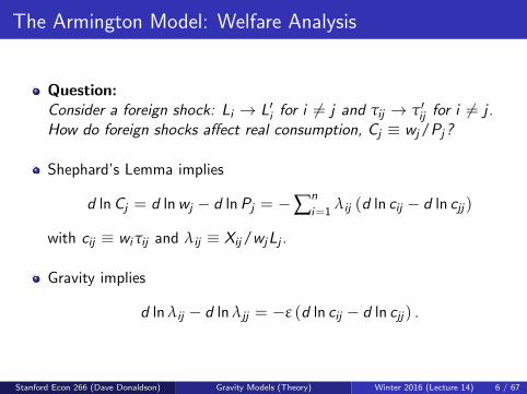
The Armington Model: Welfare Analysis

Question:Consider a foreign shock: Li → L′i for i 6= j and τij → τ′ij for i 6= j .How do foreign shocks affect real consumption, Cj ≡ wj/Pj?

Shephard’s Lemma implies

d lnCj = d lnwj − d lnPj = −∑n

i=1λij (d ln cij − d ln cjj )

with cij ≡ wiτij and λij ≡ Xij/wjLj .

Gravity implies

d ln λij − d ln λjj = −ε (d ln cij − d ln cjj ) .



Combining these two equations yields

d lnCj =∑n

i=1 λij (d ln λij − d ln λjj )

ε.

Noting that ∑i λij = 1 =⇒ ∑i λijd ln λij = 0 then

d lnCj = −d ln λjj

ε.

Integrating the previous expression yields (with x ≡ x ′/x)

Cj = λ−1/εjj .



In general, predicting λjj requires (computer) work

We can use “exact hat algebra” as in DEK (Lecture #3)Requires data on initial levels of data λij ,Yj, and εWhere to get ε? Gravity equation suggests natural (but not the only)way would be to estimate (via OLS):

lnXij = αi + αj − ε ln tij + νij

With αi as fixed-effects and tij some observable and exogenouscomponent of trade costs (that satisfies τij = tijνij ).

But predicting how bad it would be to shut down all trade is easy...

In autarky, λjj = 1. So

CAj /Cj = λ1/ε

jj

Thus gains from trade can be computed as

GTj ≡ 1− CAj /Cj = 1− λ1/ε

jj


The Armington Model: Gains from Trade

Suppose that we have estimated the trade elasticity using the gravityequation (as described above).

Central estimate in the literature is ε = 5; see Head and Mayer (2013)Handbook chapter.

Using World Input Output Database (2008) to get λjj , we can thenestimate gains from trade:

λjj % GT j

Canada 0.82 3.8

Denmark 0.74 5.8

France 0.86 3.0

Portugal 0.80 4.4

Slovakia 0.66 7.6

U.S. 0.91 1.8


Cheese, really?

The Armington Model

14.581 (Week 9) Gravity Models (Theory) Fall 2013 4 / 43


Today’s Plan






Motivation

New Trade Models

Micro-level data have lead to new questions in international trade:

How many firms export?How large are exporters?How many products do they export?

New models highlight new margins of adjustment:

From inter-industry to intra-industry to intra-firm reallocations

Old question:

How large are the gains from trade (GT)?

ACR (AER, 2012) question:

How do new trade models affect the magnitude of GT?


ACR’s Main Equivalence Result

ACR focus on gravity models

PC: Armington and Eaton & Kortum ’02MC: Krugman ’80 and many variations of Melitz ’03

Within that class, welfare changes are (x = x ′/x)

C = λ1/ε

Two sufficient statistics for welfare analysis are:

Share of domestic expenditure, λ;Trade elasticity, ε

Two views on ACR’s result:

Optimistic: welfare predictions of Armington model are more robustthan you might have thoughtPessimistic: within that class of models, micro-level data do not matter


Primitive AssumptionsPreferences and Endowments

CES utility

Consumer price index,

P1−σi =

∫ω∈Ω

pi (ω)1−σdω,

One factor of production: labor

Li ≡ labor endowment in country iwi ≡ wage in country i


Primitive AssumptionsTechnology

Linear cost function:

Cij (ω, t, q) = qwiτijαij (ω) t1

1−σ︸︷︷︸variable cost

+ w1−βi w

βj ξijφij (ω)mij (t)︸︷︷︸

fixed cost

,

q : quantity,τij : iceberg transportation cost,αij (ω) : good-specific heterogeneity in variable costs,ξij : fixed cost parameter,φij (ω) : good-specific heterogeneity in fixed costs.


Primitive AssumptionsTechnology

Linear cost function:

Cij (ω, t, q) = qwiτijαij (ω) t1

1−σ + w1−βi w

βj ξijφij (ω)mij (t)

mij (t) : cost for endogenous destination specific technology choice, t,

t ∈ [t, t] , m′ij > 0, m′′ij ≥ 0

Heterogeneity across goods

Gj (α1, ..., αn, φ1, ..., φn) ≡ ω ∈ Ω | αij (ω) ≤ αi , φij (ω) ≤ φi , ∀i


Primitive AssumptionsMarket Structure

Perfect competition

Firms can produce any good.No fixed exporting costs.

Monopolistic competition

Either firms in i can pay wiFi for monopoly power over a random good.Or exogenous measure of firms, N i < N, receive monopoly power.

Let Ni be the measure of goods that can be produced in i

Perfect competition: Ni = NMonopolistic competition: Ni < N


Macro-Level RestrictionsTrade is Balanced

Bilateral trade flows are

Xij =∫

ω∈Ωij⊂Ωxij (ω) dω

R1:For any country j ,

∑i 6=jXij = ∑i 6=j

Xji

Trivial if perfect competition or β = 0.Non trivial if β > 0.


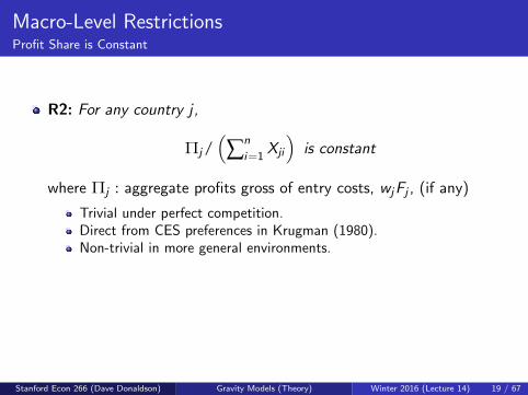
Macro-Level RestrictionsProfit Share is Constant

R2: For any country j ,

Πj/(∑n

i=1Xji

)is constant

where Πj : aggregate profits gross of entry costs, wjFj , (if any)

Trivial under perfect competition.Direct from CES preferences in Krugman (1980).Non-trivial in more general environments.


Macro-Level RestrictionsCES Import Demand System

Import demand system defined as:

(w, N, τ) → X

R3:

εii′

j ≡ ∂ ln (Xij/Xjj )/

∂ ln τi ′j =

ε < 0 i = i ′ 6= j

0 otherwise

Note: symmetry and separability.


Macro-Level RestrictionsComments on CES Import Demand System

The trade elasticity ε is an upper-level elasticity: it combines

xij (ω) (intensive margin)Ωij (extensive margin).

R3 =⇒ complete specialization.

R1-R3 are not necessarily independent

E.g., if β = 0 then R3 =⇒ R2.


Macro-Level RestrictionsStrong CES Import Demand System (AKA Gravity)

R3’: The IDS satisfies

Xij =χij ·Mi · (wiτij )

ε · Yj

∑ni ′=1 χi ′j ·Mi ′ · (wi ′τi ′j )

ε

where χij is independent of (w, M, τ).

Same restriction on εii′

j as R3 but, but additional structuralrelationships (R3’ ⇒ R3 but converse not true)


Welfare results

State of the world economy:

Z ≡ (L, τ, ξ)

Foreign shocks: a change from Z to Z′ with no domestic change.

Effects of a domestic change in Li would be different between PC andMC models (due to the home-market effect which is at work in the MCmodels but not in the PC models).


Equivalence (I)

Proposition 1: Suppose that R1-R3 hold. Then for any foreignshock it must be true that

Wj = λ1/εjj .

Implication: λjj acts as (along with elasticity ε) sufficient statistics forfully global, GE welfare analysis

Note that it is still true that for any of these models we couldestimate ε from OLS gravity regression:

lnXij = αi + αj − ε ln tij + νij

New margins affect structural interpretation of ε

...and composition of gains from trade (GT)...

... but size of GT is the same.


Gains from Trade Revisited

Proposition 1 is an ex-post result (based on seeing λjj).

A simple ex-ante result (for the case of going to autarky):

Corollary 1: Suppose that R1-R3 hold. Then

W Aj = λ−1/ε

jj .


Equivalence (II)

A stronger ex-ante result for variable trade costs (and things thatact like variable trade costs, like productivity shocks; but not for othertypes of foreign shocks) under R1-R3’:

Proposition 2: Suppose that R1-R3’ hold. Then

Wj = λ1/εjj

where

λjj =[∑n

i=1λij (wi τij )

ε]−1

,

and

wi = ∑n

j=1

λij wjYj (wi τij )ε

Yi ∑ni ′=1 λi ′j (wi ′ τi ′j )

ε .

So: ε and λij are sufficient to predict Wj (ex-ante) from τij , i 6= j .


Taking Stock

ACR consider models featuring:

(i) CES preferences;(ii) one factor of production;(iii) linear cost functions; and(iv) perfect or monopolistic competition;

with three macro-level restrictions:

(i) trade is balanced;(ii) aggregate profits are a constant share of aggregate revenues; and(iii) a CES import demand system.

Equivalence for ex-post welfare changes and GT

under R3’ equivalence carries to ex-ante welfare changesSo if R3’ is satisfied, then models in this ACR class agree on allimplications of changes in variable trade costs


A note on methodology

ACR set out to answer the question of whether different trade modelspredict different GT

In some of these cases, tempting to think that it is easy to rank GTacross these models.

E.g., following Melitz and Redding (AER, 2015), note that sinceKrugman is a strictly nested special case of Melitz for which the firmproductivity distribution is degenerate, the Melitz model is Krugmanplus an additional margin of adjustment.And since both models are efficient (i.e. correspond to planner’sproblem, so equilibrium is maximizing something), an additional marginof adjustment guarantees that the damage done by a negative shock(e.g. move to autarky) is less bad in Melitz than in Krugman.

But note that this is not the ACR thought experiment.ACR’s thought experiment is to ask about GT (or any othercounterfactual), conditional on the data λij ,Yj and elasticity ε wehave.


Today’s Plan






Departing from ACR’s (2012) Equivalence Result

Costinot and Rodriguez-Clare (Handbook of International Econ,2013) has nice discussion of general cases.

Other Gravity Models:

Multiple SectorsTradable Intermediate GoodsMultiple FactorsVariable Markups (ACDR 2012)


Multiple sectors, GT

Nested CES: Upper level EoS ρ and lower level EoS εs

Recall gains for Canada of 3.8%. Now gains can be much higher:ρ = 1 implies GT = 17.4%


Tradable intermediates, GT

Set ρ = 1, add tradable intermediates with Input-Output structure

Labor shares are 1− αj ,s and input shares are αj ,ks (∑k αj ,ks = αj ,s)


Tradable intermediates, GT

% GT j % GTMSj % GT IO

j

Canada 3.8 17.4 30.2

Denmark 5.8 30.2 41.4

France 3.0 9.4 17.2

Portugal 4.4 23.8 35.9

U.S. 1.8 4.4 8.3


Multiple sectors: a combination of micro and macrofeatures

In Krugman, free entry ⇒ scale effects associated with totalemployment

In Melitz, additional scale effects associated with sales in each market

In both models, trade may affect entry and fixed costs

All these effects do not play a role in the one sector model

With multiple sectors and traded intermediates, these effects comeback


Gains from Trade“MS” = multiple sectors; “IO” = tradable intermediates

...................................... Canada China Germany Romania US

Aggregate 3.8 0.8 4.5 4.5 1.8




Aggregate 3.8 0.8 4.5 4.5 1.8

MS, PC 17.4 4.0 12.7 17.7 4.4




Aggregate 3.8 0.8 4.5 4.5 1.8

MS, PC 17.4 4.0 12.7 17.7 4.4

MS, MC 15.3 4.0 17.6 12.7 3.8




Aggregate 3.8 0.8 4.5 4.5 1.8

MS, PC 17.4 4.0 12.7 17.7 4.4

MS, MC 15.3 4.0 17.6 12.7 3.8

MS, IO, PC 29.5 11.2 22.5 29.2 8.0




Aggregate 3.8 0.8 4.5 4.5 1.8

MS, PC 17.4 4.0 12.7 17.7 4.4

MS, MC 15.3 4.0 17.6 12.7 3.8

MS, IO, PC 29.5 11.2 22.5 29.2 8.0

MS, IO, MC (Krugman) 33.0 28.0 41.4 20.8 8.6




Aggregate 3.8 0.8 4.5 4.5 1.8

MS, PC 17.4 4.0 12.7 17.7 4.4

MS, MC 15.3 4.0 17.6 12.7 3.8

MS, IO, PC 29.5 11.2 22.5 29.2 8.0

MS, IO, MC (Krugman) 33.0 28.0 41.4 20.8 8.6

MS, IO, MC (Melitz) 39.8 77.9 52.9 20.7 10.3


Today’s Plan






Adao, Costinot and Donaldson (AER, 2016)

Without access to (much) quasi-experimental variation, traditionalapproach in the field has been to model everything: demand-side,supply-side, market structure, trade costs

E.g. #1: “Old CGE”: GTAP model [13,000 structural parameters]E.g. #2: “New CGE”: EK model [1 key parameter]

Question: Can we relax EK’s strong functional form assumptionswithout circling back to GTAP’s 13,000 parameters?


ACD (2016): 4 Steps

1 For many counterfactual questions, neoclassical models are exactlyequivalent to a reduced factor exchange economy

Reduced factor demand system sufficient for counterfactual analysis

2 Nonparametric generalization of standard gravity tools:

Dekle, Eaton and Kortum (2008): exact hat algebraArkolakis, Costinot, and Rodriguez-Clare (2012): welfare gainsHead and Ries (2001): trade costs

3 Reduced factor demand system is nonparametrically identified understandard assumptions about data/orthogonality

4 (Not today) Empirical application: What was the impact of China’sintegration into the world economy in the past two decades?

Departures from CES modeled in the spirit of BLP (1995)


Neoclassical Trade Model

i = 1, ..., I countries

k = 1, ...,K goods

n = 1, ...,N factors

Goods consumed in country i :

qi ≡ qkji

Factors used in country i to produce good k for country j :

l kij ≡ lnkij


Neoclassical Trade Model

Preferences: ui = ui (qi )

Representative consumer (driven by data from “country” i)

Technology: qkij = f kij (lkij )

Non-increasing returns to scale. No joint production.Extensions in paper to include (global/domestic) input-output linkagesand tariffs/taxes/subsidies.

Factor endowments: νni > 0

Defined as the (set of imperfectly substitutable) inputs to productionthat are in fixed supply.


Competitive Equilibrium

A q ≡ qi, l ≡ li, p ≡ pi, and w ≡ wi such that:

1 Consumers maximize their utility:

qi ∈ argmaxqiui (qi )

∑j ,k

pkji qkji ≤∑

n

wni νni for all i ;

2 Firms maximize their profits:

l kij ∈ argmaxl kijpkij f kij (l kij )−∑

n

wni l

nkij for all i , j , and k;

3 Goods markets clear:

qkij = f kij (lkij ) for all i , j , and k;

4 Factors markets clear:

∑j ,k

lnkij = νni for all i and n.


Reduced Exchange Model

Fictitious endowment economy in which consumers directly exchangefactor services

Taylor (1938), Rader (1972), Wilson (1980), Mas-Colell (1991)

Reduced preferences over primary factors of production:

Ui (Li ) ≡ maxqi ,li ui (qi )

qkji ≤ f kji (lkji ) for all j and k ,

∑k

lnkji ≤ Lnji for all j and n,

Easy to check that Ui (·) is strictly increasing and quasiconcave.

Not necessarily strictly quasiconcave, even if ui (·) is.Example: H-O model inside FPE set.


Reduced Equilibrium

Corresponds to L ≡ Li and w ≡ wi such that:

1 Consumers maximize their reduced utility:

Li ∈ argmaxLiUi (Li )

∑j ,n

wnj L

nji ≤∑

n

wni νni for all i ;

2 Factor markets clear:

∑j

Lnij = νni for all i and n.


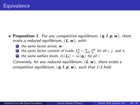
Equivalence

Proposition 1: For any competitive equilibrium, (q, l , p, w ), thereexists a reduced equilibrium, (L, w ), with:

1 the same factor prices, w ;2 the same factor content of trade, Lnji = ∑k l

nkji for all i , j , and n;

3 the same welfare levels, Ui (Li ) = ui (qi ) for all i .

Conversely, for any reduced equilibrium, (L, w ), there exists acompetitive equilibrium, (q, l , p, w ), such that 1-3 hold.


Equivalence

Comments:Proof is similar to First and Second Welfare Theorems. Key distinctionis that standard Welfare Theorems go from CE to global planner’sproblem, whereas RE remains a decentralized equilibrium (but one inwhich countries fictitiously trade factor services and budget is balancedcountry by country).

Key implication of Prop. 1: If one is interested in the factor content oftrade, factor prices and/or welfare, then one can always study a REinstead of a CE. One doesn’t need direct knowledge of primitives u andf but only of how these indirectly shape U.


Reduced Counterfactuals

Suppose that the reduced utility function over primary factors in thiseconomy can be parametrized as

Ui (Li ) ≡ Ui (Lnji/τnji ),

where τnji > 0 are exogenous preference shocks

Counterfactual question: What are the effects of a change from(τ, ν) to (τ′, ν′) on trade flows, factor prices, and welfare?


Reduced Factor Demand System

Start from factor demand = solution of reduced UMP:

Li (w , yi |τi )

Compute associated expenditure shares:

χi (w , yi |τi ) ≡ xnji |xnji = wnj L

nji/yi for some Li ∈ Li (w , yi |τi )

Rearrange in terms of effective factor prices, ωi ≡ wnj τn

ji :

χi (w , yi |τi ) ≡ χi (ωi , yi )


Reduced Equilibrium

In this notation, RE is:

xi ∈ χi (ωi , yi ), for all i ,

∑j

xnij yj = yni , for all i and n

Gravity model (i.e. ACR): Reduced factor demand system is CES

χji (ωi , yi ) =(ωji )ε

∑l (ωli )ε, for all j and i


Exact Hat Algebra

Start from the counterfactual equilibrium:

x ′i ∈ χi (ω

′i , y′i ) for all i ,

∑j

(xnij )′y ′j = (yni )

′, for all i and n.

Rearrange in terms of proportional changes:

xnji xnji ∈ χi (wnj τn

ji ωnji, ∑

n

wni νni y

ni ) for all i ,

∑j

xnij xnij (∑

n

wnj νnj y

nj ) = wn

i νni yni , for all i and n.


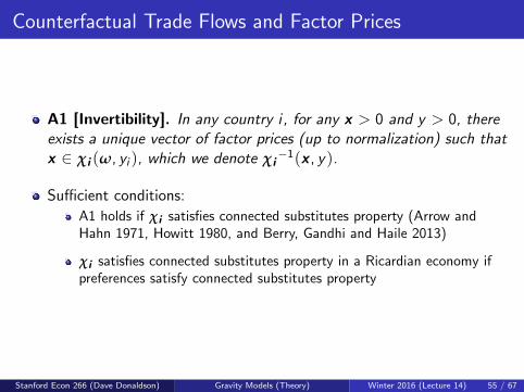
Counterfactual Trade Flows and Factor Prices

A1 [Invertibility]. In any country i , for any x > 0 and y > 0, thereexists a unique vector of factor prices (up to normalization) such thatx ∈ χi (ω, yi ), which we denote χi

−1(x , y).

Sufficient conditions:

A1 holds if χi satisfies connected substitutes property (Arrow andHahn 1971, Howitt 1980, and Berry, Gandhi and Haile 2013)

χi satisfies connected substitutes property in a Ricardian economy ifpreferences satisfy connected substitutes property



Proposition 2 Under A1, proportional changes in expenditure sharesand factor prices, x and w , caused by proportional changes inpreferences and endowments, τ and ν, solve


ji ωnji, ∑

n

wni νni y

ni ) ∀ i ,

∑j

xnij xnij (∑

n

wnj νnj y

nj ) = wn

i νni yni ∀ i and n.



Proposition 2 Under A1, proportional changes in expenditure sharesand factor prices, x and w , caused by proportional changes inpreferences and endowments, τ and ν, solve


ji (χnji )−1(xi , yi ), ∑

n

wni νni y

ni ) ∀ i ,

∑j

xnij xnij (∑

n

wnj νnj y

nj ) = wn

i νni yni ∀ i and n.


Welfare

Equivalent variation for country i associated with change from (τ, ν)to (τ′, ν′), expressed as fraction of initial income:

∆Wi = (ei (ωi ,U′i ))− yi )/yi ,

with U ′i = counterfactual utility and ei = expenditure function,

ei (ωi ,U′i ) ≡ minLi ∑ ωn

jiLnji

Ui (Li ) ≥ U ′i .


Integrating Below Factor Demand Curves

To go from χi to ∆Wi , solve system of ODEs

For any selection xnji (ω, y) ∈ χi (ω, y), Envelope Theorem:

d ln ei (ω,U ′i )

d ln ωnj

= xnji (ω, ei (ω,U ′i )) for all j and n.

Budget balance in the counterfactual equilibrium

ei (ω′i ,U

′i ) = y ′i .


Counterfactual Welfare Changes

Proposition 3 Under A1, equivalent variation associated with changefrom (τ, ν) to (τ′, ν′) is

∆Wi = (e((χnji )−1(xi , yi ),U ′i )− yi )/yi ,

where e(·,U ′i ) is the unique solution of (1) and (2).


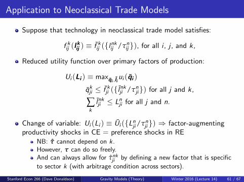
Application to Neoclassical Trade Models

Suppose that technology in neoclassical trade model satisfies:

f kij (lkij ) ≡ f kij (lnkij /τn

ij ), for all i , j , and k ,

Reduced utility function over primary factors of production:

Ui (Li ) ≡ maxqi ,li ui (qi )

qkji ≤ f kji (lnkji /τnji) for all j and k ,

∑k

lnkji ≤ Lnji for all j and n.

Change of variable: Ui (Li ) ≡ Ui (Lnji/τnji ) ⇒ factor-augmenting

productivity shocks in CE = preference shocks in RENB: τ cannot depend on k .However, τ can do so freely.And can always allow for τnk

ji by defining a new factor that is specific

to sector k (with arbitrage condition across sectors).


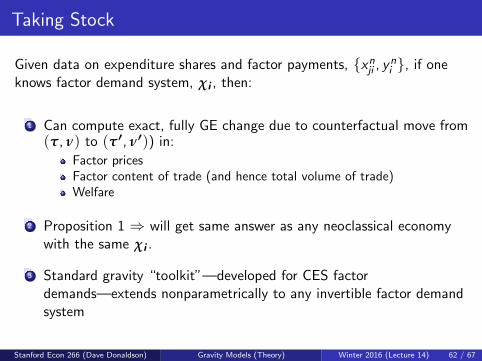
Taking Stock

Given data on expenditure shares and factor payments, xnji , yni , if oneknows factor demand system, χi , then:

1 Can compute exact, fully GE change due to counterfactual move from(τ, ν) to (τ′, ν′)) in:

Factor pricesFactor content of trade (and hence total volume of trade)Welfare

2 Proposition 1 ⇒ will get same answer as any neoclassical economywith the same χi .

3 Standard gravity “toolkit”—developed for CES factordemands—extends nonparametrically to any invertible factor demandsystem


Identification Assumptions: Shocks

Data generated by neoclassical trade model at different dates t

At each date, preferences and technology such that:

ui (qi ,t) = u(qkji ,t/θji), for all i ,

f kij ,t(lkij ,t) = f ki (lnkij ,t/τn

ij ,t), for all i , j , and k .

A2. [Price heterogeneity] In any country i and at any date t, thereexists ωi ,t ≡ wn

j ,tθjiτnji ,t, such that factor demand can be expressed

as χ(ωi ,t , yi ,t).


Identification Assumptions: Exogeneity

Observables:1 xnji ,t : factor expenditure shares (normal FCT data in principle; but

non-trivial aggregation bias issues in practice)2 yni ,t : factor payments3 znji ,t : factor price shifters (e.g. observable shifter of trade costs)

Effective factor prices, ωji ,t , unobservable, but related to znji ,t :

lnωnji ,t = ln znji ,t + ϕn

ji + ξnj ,t + εnji ,t , for all i , j , n, and t

A3. [Exogeneity] E [εi ,t | ln zi ,t , di ,t ] = 0, where di ,t is a vector ofimporter-exporter-factor dummies and exporter-factor-year dummieswith i = importer and t = year for all dummies.


Identification Assumptions: Completeness

Following Newey and Powell (2003), we conclude by imposing thefollowing completeness condition.

A4. [Completeness] For any g(xi ,t , yi ,t),E [g(xi ,t , yi ,t)| ln zi ,t , di ,t ] = 0 implies g(xi ,t , yi ,t) = 0.

A4 = rank condition in estimation of parametric models.


Identifying Factor Demand

A1 ⇒ωn

ji ,t = (χnji )−1(xi ,t , yi ,t).

Taking logs and using definition of εnji ,t :

εnji ,t = ln(χnji )−1(xi ,t , yi ,t)− ln znji ,t − ϕn

ji − ξnj ,t .

A2 ⇒εnji ,t = ln(χn

j )−1(xi ,t , yi ,t)− ln znji ,t − ϕn

ji − ξnj ,t .

Using A3, we obtain the following moment condition

E [ln(χnj )−1(xi ,t , yi ,t)− ln znji ,t − ϕn

ji − ξnj ,t | ln zi ,t , di ,t ] = 0.

A4 ⇒ unique solution (χnj )−1 to (3) (up to a normalization)


Identifying Factor Demand

Once the inverse factor demand is known, both factor demand andeffective factor prices are known as well, with prices being uniquelypinned down (up to a normalization).

Proposition 4 Suppose that A1-A4 hold. Then effective factor pricesωi ,t and the factor demand system χ are identified (up to anormalization).


Date post:	10-Jun-2018
Category:	Documents
Upload:	lehanh
View:	216 times
Download:	0 times

Lecture 14: Gravity Models (Theory) - Dave...

Documents