Lecture 2: The Mechanics of 4D-Var

Outline

• The conjugate gradient algorithm• Preconditioning• Covariance modeling• Background quality control

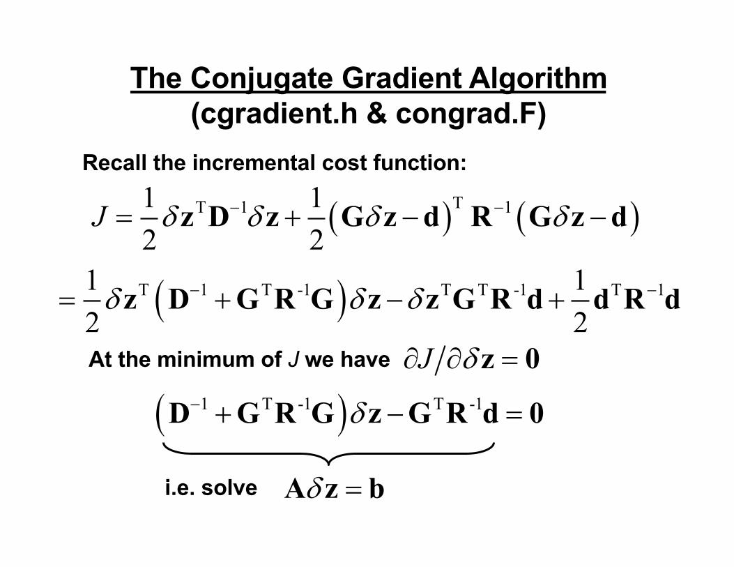
The Conjugate Gradient Algorithm(cgradient.h & congrad.F)

( ) ( )TT 1 11 12 2

J d d d d- -= + - -z D z G z d R G z d

Recall the incremental cost function:

( )T 1 T -1 T T -1 T 11 12 2d d d- -= + - +z D G R G z z G R d d R d

At the minimum of J we have J d¶ ¶ =z 0

( )1 T -1 T -1d- + - =D G R G z G R d 0

d =A z bi.e. solve

The Conjugate Gradient AlgorithmThe ECMWF “congrad” of Fisher (1997) for inner-loop k+1:

ˆ k k k kd d t= +z z h trial step

ˆ ˆk kJ d= ¶ ¶g z gradient @ trial step

( )T T ˆ/ ( )k k k k k k ka t= - -h g h g g optimum step

1k k k kd d a+ = +z z h new starting point

( )1 ˆ( / )k k k k k ka t+ = + -g g g g gradient @new point

T T1 1 1 /k k k k kb + + += g g g g

1 1 1k k k kb+ + += - +h g h new descent direction

TL & AD ROMS

CorneliusLanczos

(1893-1974)

The Lanczos Connection

The Lanczos Connection

1 1 2 1 1k k k k k k kg d g+ + + + += + +Aq q q qThe CG algorithm is equivalent to:

“Lanczos recursion relation”

1 2k+1 1 1 k 1; (1 ); k k k k k k k kd a b a g b a+ + += = + = -q g g

T1k k k k k kg += +AV V T q e

1 1

1 2 2

2 1 1

1

k

k k k

k k

d gg d g

g d gg d

- - -

-

æ öç ÷ç ÷ç ÷=ç ÷ç ÷ç ÷è ø

T ! ! ! !

! !

OrthonormalLanczos vectors

Ti j ijd=q q

Vk = qi( )

VkTVk = Ik

The Lanczos Connection

A ≈ VkTkVkT

A−1 ≈ VkTk−1Vk

T

Specifically:

The Lanczos Connection

Gain (primal form):1 T 1 1 T 1( )- - - -= +K D G R G G R

-1 T T 1k k k k

-=K V T V G R!

Practical gain matrix:

Useful for diagnostic applications (Lecture 5)(The Lanczos vectors are in ADJname)

Preconditioning

J J

preconditioning

µ µAs=µs

Preconditioning seeks to cluster the eigenvalues of Avia a transformation of variable

Preconditioning

At the minimum of J we have J d¶ ¶ =z 0

( )1 T -1 T -1d- + - =D G R G z G R d 0d =A z bi.e. solve

Introduce a new variable: 1 2d=v A z

T T12

J cd d d= - +z A z z bMinimize:

T T T 212

J c-= - +v v v A bT 2J -¶ ¶ = - =v v A b 0At the minimum:

Preconditioning

( ) ( )TT 1 11 12 2

J d d d d- -= + - -z D z G z d R G z d

Recall the incremental cost function:

Introduce a new variable: 1 2d-=v D z

( ) ( )TT 1 2 1 1 21 1( )2 2

J -= + - -v v v GD v d R GD v d

( )T 1 2 T -1 1 2 T 1 2 T -1 T 11 12 2

-= + - +v I D G R GD v v D G R d d R d

At the minimum of J we have J¶ ¶ =v 0

( )1 2 T -1 1 2 1 2 T -1+ - =I D G R GD v D G R d 0=Av b! !i.e. solve then 1 2d =z D v

=Av b! !

Preconditioning

( )1 2 T -1 1 2= +A I D G R GD!

Solve

Has eigenvaluesclustered around 1

( )J d z ( )J v

The Conjugate Gradient Algorithmcgradient.h in v-space to minimize

ˆ k k k kt= +v v h trial step

T 2ˆ ˆk kJ d= ¶ ¶g D z gradient @ trial step

( )T T ˆ/ ( )k k k k k ka t= - - kh g h g g optimum step

1k k k ka+ = +v v h new starting point

( )1 ˆ( / )k k k k k ka t+ = + -g g g g gradient @new point

T T1 1 1 /k k k k kb + + += g g g g

1 1 1k k k kb+ + += - +h g h new descent direction

( )J v

1 21 1k kd + +=z D v project into state-space

The Lanczos Connection

Gain (primal form):1 2 T 2 T 1 1 2 1 T 2 T 1( )- - -= +K D I D G R GD D G R

1 2 -1 T T 2 T 1k k k k

-=K D V T V D G R!

Practical gain matrix:

Useful for diagnostic applications (Lecture 5)(The Lanczos vectors are in ADJname)

Covariance Modeling

( ) ( )TT 1 11 12 2

J d d d d- -= + - -z D z G z d R G z d

Recall the incremental cost function:

At the minimum of J we have J d¶ ¶ =z 0

( )1 T 1J d d d- -¶ ¶ = + -z D z G R G z d

bJ oJ

where diag( , , , )= x b fD B B B Q

Covariance Modeling

Bx = initial condition prior (or background) errorcovariance matrix

Bf = surface forcing prior error covariance matrixBb = open boundary condition prior error covariance

matrixQ = prior model error covariance matrix

Each covariance matrix is factorized according to:T T= b bB K ΣCΣ K

C = univariate correlation matrixS = diagonal matrix of error standard deviationsKb = multivariate balance operator (for Bx and Q only)

Correlation Models

C is further factorized as:

1 2 1 2 -1 T 2 T 2 T= v h h vC ΛL L W L L Λ

W = diagonal matrix of grid box volumesLh = horizontal correlation function modelLv = vertical correlation function modelL = matrix of normalization coefficients

Lh and Lv are based on solutions of 2D and 1Dpseudo diffusion equations respectively:

2 0hth k h¶ ¶ - Ñ = 2 2 0vt zh k h¶ ¶ - ¶ ¶ =

iW

Correlation Models

C is further factorized as:

1 2 1 2 -1 T 2 T 2 T= v h h vC ΛL L W L L Λ

W = diagonal matrix of grid box volumesLh = horizontal correlation function modelLv = vertical correlation function modelL = matrix of normalization coefficients

Lh and Lv are based on solutions of 2D and 1Dpseudo diffusion equations respectively:

2 0hth k h¶ ¶ - Ñ = 2 2 0vt zh k h¶ ¶ - ¶ ¶ =

Correlation Models

t=0 t=T

2 2L Tk»Correlation length, L:

x Cx

Covariance Modeling

1 2 1 2 -1 T 2 T 2 T= v h h vC ΛL L W L L Λ

L ensures that the range of C is ±1.

( ) T=x uB ΣCΣ

Suppose that x is divided into a balanced and unbalancedcontribution: x=xb+xu

Examples of balance relations: geostrophy, hydrostatic

( ) T=x b x buB K B K

The Balance Operator(define BALANCE_OPERATOR)

dd

d ddd

é ùê úê úê ú=ê úê úê úë û

TS

x ζuv

Totalstate

vectorincrements

ˆ

dddddd

é ùê úê úê ú=ê úê úê úë û

u

u

u

u

TSζxuv

Unbalancedstate

vectorincrements

(except for dT)

ˆd d= bx K x( ) Tˆ ˆd d=x uB x x

( )

T

T T

T

ˆ ˆ

d d

d d

=

=

=

x

b b

b u bx

B x x

K x x K

K B K

Following Weaver et al (2005):

The Balance Operator

STd d d= + uS K T S

VrdV dr dV= + uK

upd d d= + uu K p u

vpd d d= + uv K p v

T Sr rdr d d= +K T K S

p pr Vd dr dV= +p K K

T-S relation

Level of no motion or elliptic eqn

Geostrophic balance

Geostrophic balance

Linear equation of state

Hydrostatic balance

ST

T S

uT uS u

vT vS v

V V

V

V

æ öç ÷ç ÷ç ÷=ç ÷ç ÷ç ÷è ø

b

I 0 0 0 0K I 0 0 0K K I 0 0KK K K I 0K K K 0 I

The Balance Operator

ˆd d= bx K x

The Balance Operator

STK from prior (background) T-S relationship

bS T

S zS Tz T

d g d¶ ¶=

¶ ¶

0 depending on mixed layer

1g

ü= ý

þ

ST

T S

uT uS u

vT vS v

V V

V

V

æ öç ÷ç ÷ç ÷=ç ÷ç ÷ç ÷è ø

b

I 0 0 0 0K I 0 0 0K K I 0 0KK K K I 0K K K 0 I

The Balance Operator

The Balance Operator

( )T T S STV Vr r r= +K K K K K

S SV Vr r=K K K( )0 T Sdr r ad bd= - +

0

0/r

bz

dzdV dr r= -ò (level of no motion zr)

0 0

0( ) / ' ...b h zh dz dzdV dr r

-Ñ Ñ = -Ñ +ò ò

Either:

(i)

(ii)

(define ZETA_ELLIPTIC)

ST

T S

uT uS u

vT vS v

V V

V

V

æ öç ÷ç ÷ç ÷=ç ÷ç ÷ç ÷è ø

b

I 0 0 0 0K I 0 0 0K K I 0 0KK K K I 0K K K 0 I

The Balance Operator

The Balance Operator

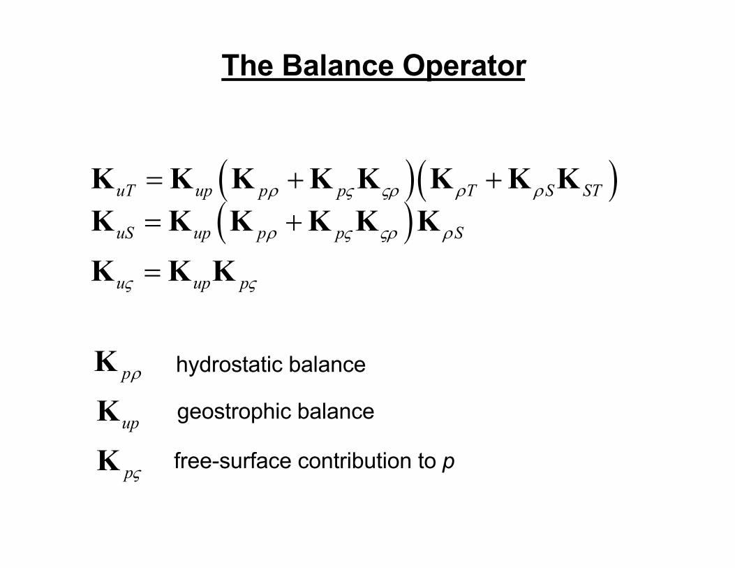
( )( )uT up p p T S STr V Vr r r= + +K K K K K K K K

prK

upKhydrostatic balance

geostrophic balance

( )uS up p p Sr V Vr r= +K K K K K K

u up pV V=K K K

pVK free-surface contribution to p

( ) T

T T T TTT ST T uT vT

T T TST SS S uS vS

T TT S u v

TuT uS u uu vu

vT vS v vu vv

V

V

V V VV V V

V

V

æ öç ÷ç ÷ç ÷= =ç ÷ç ÷ç ÷è ø

x b x bu

B B B B BB B B B B

B K B K B B B B BB B B B BB B B B B

The Balance Operator

IS4DVAR Balanced Operator Covariances: EAC

The cross-covariances are computed from a single sea surface height observation using multivariate physical balance relationships.

Free-surface(m)2

Temperature(Celsius)2

Salinity(nondimensional)2

U-velocity(m/s)2

V-velocity(m/s)2

Z = -300m Z = -300m Z = -300m Z = -300m

IS4DVAR Balanced Operator Covariances: EAC

Free-surface(m)2

Temperature(Celsius)2

Salinity(nondimensional)2

U-velocity(m/s)2

V-velocity(m/s)2

The cross-covariances are computed from a single temperatureobservation at the surface using multivariate physical balance relationships.

Z = 0m Z = -300m Z = -300m Z = -300m

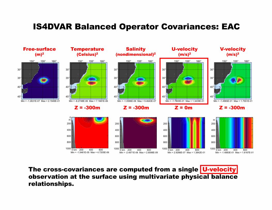
IS4DVAR Balanced Operator Covariances: EAC

Free-surface(m)2

Temperature(Celsius)2

Salinity(nondimensional)2

U-velocity(m/s)2

V-velocity(m/s)2

The cross-covariances are computed from a single U-velocityobservation at the surface using multivariate physical balance relationships.

Z = -300m Z = -300m Z = 0m Z = -300m

T T=x b x x x bB K Σ C Σ K

T=f f f fB Σ C Σ

T=b b b bB Σ C Σ

T T= b q q q bQ K Σ C Σ K

No balance

No balance

Initial condition prior:

Surface forcing prior:

Open boundary condition prior:

Model error prior:

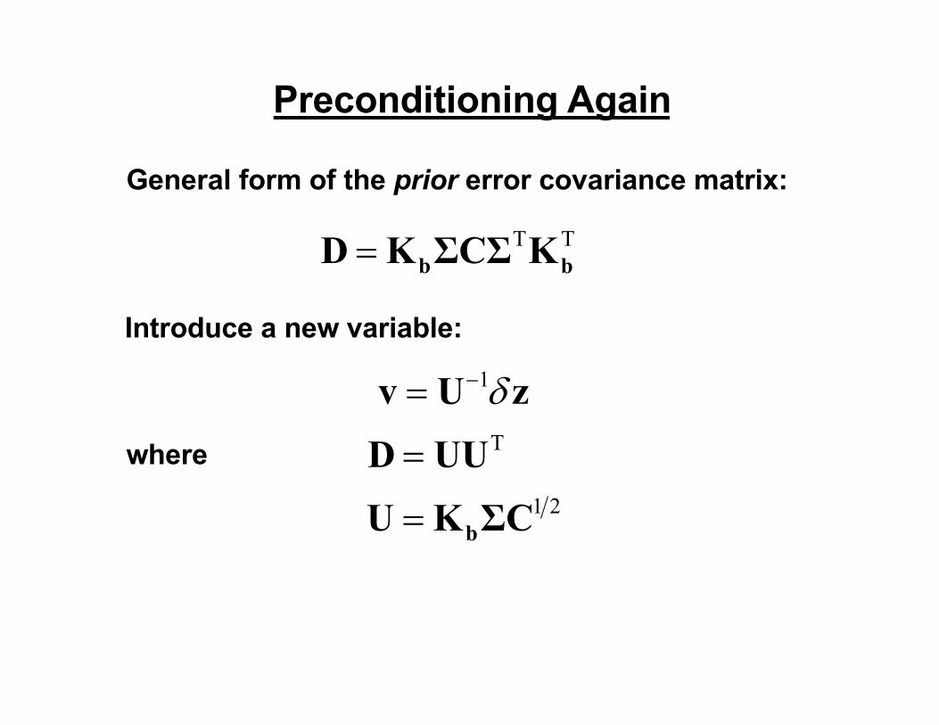
Preconditioning Again

Introduce a new variable:1d-=v U z

T T= b bD K ΣCΣ K

General form of the prior error covariance matrix:

where T=D UU1 2= bU K ΣC

The Conjugate Gradient Algorithmcgradient.h in v-space to minimize

ˆ k k k kt= +v v h trial step

T 2 T Tˆ ˆk kJ d= ¶ ¶bg C Σ K z gradient @ trial step

( )T T ˆ/ ( )k k k k k ka t= - - kh g h g g optimum step

1k k k ka+ = +v v h new starting point

( )1 ˆ( / )k k k k k ka t+ = + -g g g g gradient @new point

T T1 1 1 /k k k k kb + + += g g g g

1 1 1k k k kb+ + += - +h g h new descent direction

( )J v

1 21 1k kd + += bz K ΣC v project into state-space

The Lanczos Connection

Gain (primal form):1 2 T 2 T 1 1 2 T 2 T T T 1( )- - -= + 1

b bK K ΣC I D G R GD C Σ K G R

1 2 -1 T T 2 T T T 1k k k k

-= b bK K ΣC V T V C Σ K G R!

Practical gain matrix:

Useful for diagnostic applications (Lecture 5)(The Lanczos vectors are in ADJname)

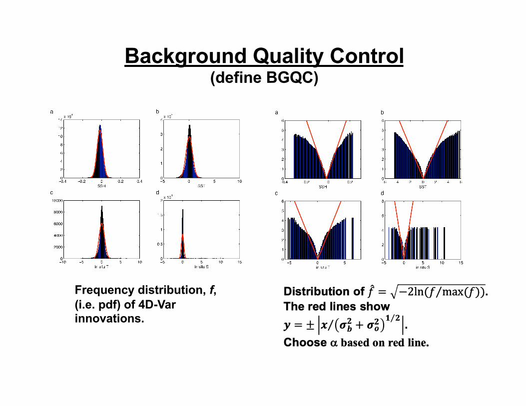
Background Quality Control(define BGQC)

• Some observations will be outliers for a variety of reasons (e.g. bad obs, bad model, or both, non-Gaussian behavior, etc)

• It is important to exclude these data from the data assimilation system since they can adversely affect the analysis.

• Observations are screened in ROMS according to the background error and observation error variances.

• The approach used in ROMS parallels that used in the ECMWF NWP system.

• An observation is rejected if the normalized innovation exceeds a specified multiple of the standard expected error.

• Specifically:

• a is a user-specified parameter.(see Andersson and Järvinen (1999, QJRMS, 125, 697-722).

yi − Hi xb( )( )2 >α 2 1+σ o2 σ b

2( )

Background Quality Control(define BGQC)

Frequency distribution, f, (i.e. pdf) of 4D-Var innovations.

Issues & Things to do

• Relax horizontal homogeneity and isotropy ofLx and Ly correlation lengths.

• Elliptic solver for free-surface balance:- cannot handle islands at the moment- add additional boundary condition option

• Cannot assimilate obs right at the open boundary.• Div and curl of dt are not constrained.• No restart option for 4D-Var.• Variational bias correction.• Variational QC.

Summary• Lanczos formulation of CG: cgradient.h• Lanczos vectors saved in ADJname• Covariance models using diffusion operators:

define VCONVOLUTIONdefine IMPLICIT_VCONV, etc

- tl_variability.F- ad_variability.F- tl_convolution.F- ad_convolution.F

• Multivariate balance operator:define BALANCE_OPERATOR

- tl_balance.F- ad_balance.F

• Background QC: define BGQC

bKTbK

ΣTΣ1 2CT 2C

References• Andersson, E. and H. Järvinen, 1999: Variational quality control. Q.

J. R. Meteorol. Soc., 125, 697-722.• Fisher, M., 1997: Minimization algorithms for variational data

assimilation. ECMWF Technical Reports, “Recent Advances in Numerical Atmospheric Modelling.”

• Tshimanga, J., S. Gratton, A.T. Weaver and A. Sartenaer, 2008: Limited-memory preconditioners with application to incremental variational data assimilation. Q. J. R. Meteorol. Soc., 134, 751-769.

• Weaver, A.T. and P. Courtier, 2001: Correlation modelling on the sphere using a generalized diffusion equation. Q. J. R. Meteorol. Soc., 127, 1815-1846.

• Weaver, A.T., C. Deltel, E. Machu, S. Ricci and N. Daget, 2005: A multivariate balance operator for variational ocean data assimilation. Q. J. R. Meteorol. Soc., 131, 3605-3625.