Lecture Notes in Biomathematics Managing Editor: S. Levin

A. Hastings (Ed.)

Community Ecology A Workshop held at Davis, CA, April 1986

S pringer-Verlag Berlin Heidelberg NewYbrk London Paris Tokyo

CHAPTER 6 Untangling 'An Entangled Bank':

Recent Facts and Theories About Community Food Webs

Joel E. Cohen Rockefeller University, 1230 York Avenue, New York, NY 10021-6399, U.S.A.

I. INTRODUCTION

This paper is an expository and nontechnical review of some recent discoveries about food webs. The discoveries are those I have been privileged to make jointly with two splendid collaborators: FrklCric Briand, formerly at the University of Ottawa and now at the International Union for the Conservation of Nature, Gland, Switzerland; and Chiules M. Newman, at the University of Arizona, Tucson. These discoveries depend on data collected by scores of field ecologists, so the circle of contributors is much wider.

I do not attempt here a panoramic review of community ecology (for which, see e.g. Diamond and Case, 1986; Kikkawa and Anderson, 1986), or even of food webs (see Pimm, 1982, and this volume; DeAngelis et al., 1983). I attempt rather to describe in a simple way some new facts that, in their original presentations, may appear forbiddingly technical. I hope that, in the future, a thorough theoretical understanding of these facts, and of models that can provide quantitative explanations of them, will lead eventually to quantitative understanding of many other empirically justified approaches to food webs (e.g. Cohen, 1978; Pimm, Chapter 7, this volume; Sugihara, 1984).

Food webs describe which species of organisms in a community eat which other species, if any. Food webs figure in one of the most famous paragraphs in biology, the last paragraph of Charles Darwin's book, "On the Origin of Species." That paragraph begins: "It is

interesting to contemplate an entangled bank, clothed with many plants of many kinds, with birds singing on the bushes, with various insects flitting about, and with worms crawling through the damp earth, and to reflect that these elaborately constructed forms, so different from each other, and dependent on each other in so complex a manner, have all been produced by laws acting around us." Darwin summarizes his theory of evolution and resumes: "Thus, from the war of nature, from famine and death, the most exalted object which we [Darwin speaks anthropocentrically here] are capable of conceiving, namely, the production of the higher animals, directly follows." The study of food webs is the study of that war of nature, and of the laws acting around us which govern it.

So far as I know, food webs were first described in scientific detail at the beginning of this century. Now, more than a century and a quarter after Darwin published his theory of evolution, enough examples of the war of nature have been patiently observed and recorded to make it possible to understand how the lines of battle are drawn. I will illustrate what a food

web is and how a food web is described. Even relatively simple webs may seem very complex, too complex to understand

whole.. Until recent decades,ecological theorists studied small components of webs, such as , . ._,. . , - . . .... . ' . , .i ;. ,. . >. - ' '.' '. ' .:. . -. . . ., . . .. .. . . ." . . . . - ',

interactions between a.pr&dator species.and a piey species: 1, have, tirued in th.&opiosite "' . ' '

direction, in the hope that ensembles or collections of food webs might display simple general properties that are not evident from any single web. This hope, after the long labors of gathering and analyzing data on many webs, has been fulfilled. I will present some quantitative empirical generalizations that we have recently discovered about food webs.

Then I will present two models. One of the models unifies the quantitative generalizations. This successful model is ridiculously simple. Any self-respecting field ecologist would sneer at it. (Rightly so: Where are its dynamics, its spatial structure, its representation of behavior and genetics and physiology and energy flow and environmental fluctuations?) I present it only because no other model at present connects and explains quantitatively what is observed. We call the successful model the cascade model. After showing that the cascade model describes what we know already, I then show that it makes novel predictions about things we did not know already: These predictions can be tested.

Finally, I will outline some potential uses of facts and t,heixies about food webs.

11. TERMS Let me introduce some terms and illustrate them with an example. A food web is a

collection of trophic species, together with their feeding relations. A trophic species is a collection of organisms that have the same diets and the same predators. A biological species, in the usual use of the term, refers to a collection of organisms with shared genetics. A trophic species will sometimes be a biological species, but not always. A trophic species may be a biological species of plait or animal, or several species, or a stage in the life cycle of one biological species. Hereafter, the word "species" means "trophic species."

Each arrow in a food web goes from food to eater, or from prey to predator. I call each arrow a "link", short for "trophic link."

Fig. 1 is a picture of the food web on an island in the Pacific Ocean. Some species are top, meaning that no other species in the web eats them, e.g., reef heron, starlings. Notice that the web omits decomposers. Some species are intermediate, meaning that at least one species eats them, and they eat at least one species, e.g., insects, skinks, fish. Some species are basal, meaning that they eat no other species, e.g., algae, phytoplankton. To quantify the structure of webs, we count the numbers of species that are top, intermediate and basal.

These three kinds of species specify four kinds of links: basal-intermediate links, e.g., phytoplankton to zooplankton; basal-top links, e.g., coconut to man; intermediate-intermediate links, e.g., zooplankton to fish; and intermediate-top links, e.g., fish to frigate birds. We also count the numbers of links of each of these four kinds.

Fig.1 Food web in the Kapingamarangi Atoll. From p. 157 of Niering, 1963.

.<':+. :'. -,.r, . - ..*' . .,. . .- 4:.. , , *> .... , . . ,. . ..,., . .- ..- . ' ..' ! . , t' ,. - . . . * '

A chain is a path of links from a basal species to a top species, e.g., phytoplankton to fish to terns. The length of a chain is the number of links in it. In Fig. 1, the longest chain has only four lit$?, and there, is pnly ,cne. chak.of 1ength.four. Short chaing,?e typi~al,,of

, -,: ". r.; ., '..,. . . :' .-.: .- ., '. ..-.. < . ,..,.. ..... ,. :.., :.; ;. ..,.* ;'> . *;.., ? > ... ':. .,., ?::> - r -'.;. . :,.. , .. .,,:*,,:*,..? .;:ki:f I ' .>.. . _. . , . ..: . . . I . .

,webs. ' . . , . . .. . A cycle is a directed sequence of one or more links starting from, and ending at, the

same species. A cycle of length 1 describes cannibalism, in which a species eats itself. Cannibalism is common in nature. But ecologists report cannibalism so unreliably that we have simply suppressed it from all the data even where it is reported. A cycle of length 2 means that A eats B and B eats A. In this example, as in most webs, there are no cycles of length 2 or more.

In summary, the terms just defined are trophic species, including top, intermediate and basal; links, including basal-intermediate, basal-top, intermediate-intermediate and intermediate-top; and chains, length (the number of links) and cycles.

111. LAWS Here are five'laws or empirical generalizations about food webs. .' First, excluding cannibalism, cycles are rare. This generalization, without detailed

supporting data, was offered as long ago as 1972 (Gallopin, 1972). Of 113 webs, three webs each contained a single cycle of length 2, and there were no other cycles (Cohen and Newman, 1985, p. 426; Cohen, Briand and Newman, 1986, p. 333).

Second, chains are short (Hutchinson, 1959). If one finds the maximum chain length within each web, then the median of this maximum in the 113 webs in the collection studied by Cohen, Briand, and Newman (1986) is four links and the upper quartile of the maximum chain length is five links. The longest chains in all 113 webs had ten links, and only one web had chains that long.

The last three laws deal with scale invariance (Cohen, 1977; Briand and Cohen, 1984; Cohen and Briand, 1984). We have compared the form of webs of different sizes. Such a comparison might be called the allometry of food webs. To appreciate the significance of what we found, consider a baby's face. The location of the eyes with respect to the top and the bottom of the head differs from the location of the eyes in an adult's face. That means that as the size of the face increases, the proportions change. I'm going to describe three laws which report that food webs, unlike a baby's face, have the same shape at different sizes.

Scale invariance means that food webs of different size have constant proportions. Our third law is scale invariance in three ratios: numbers of top species in proportion

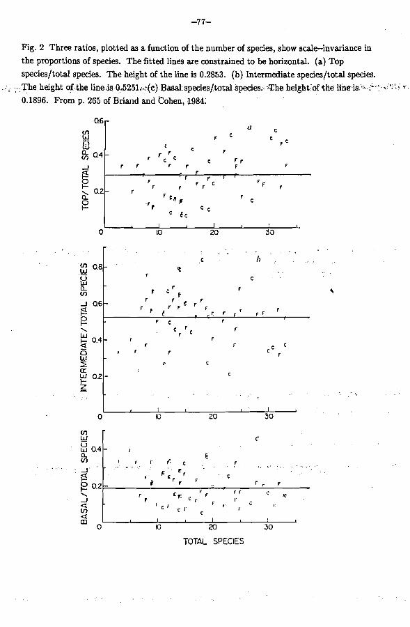
to numbers of all species; numbers of intermediate species in proportion to numbers of all species; and numbers of basal species in proportion to numbers of all species. Fig. Yshows iw

the proportions of all species that are top species, intermediate species and basal species. There's evidently no increasing or decreasing trend as the number of species increases (Briand and Cohen, 1984). The variability of proportions with respect to the

average could be explained by chance alone. One can summarize crudely by saying that about a quarter (29 percent) of all species are top, about half (53 percent) are intermediate and ...; . . - . about a quarter (19 percent) df the s&cies';ne basal.. ere, scale invariance desciibes the observation that as the number of species ill62 webs varies from 0 to 33, the proportions of top, intermediate and basal species apparently remain invariant.

Our fourth law is scale invariance in the proportions of the different kinds of links. In Fig. 3a (Cohen and Briand, 1984), for example, the abscissa is the number of species 4 and the

ordinate is the proportion of basal-intermediate links among all links. There is no clear evidence of an increasing or decreasing trend. The proportions of different kinds of links, like the proportions of species, are approximately scale-invariant. Here the scatter about a horizontal line is too big to be explained by random sampling.

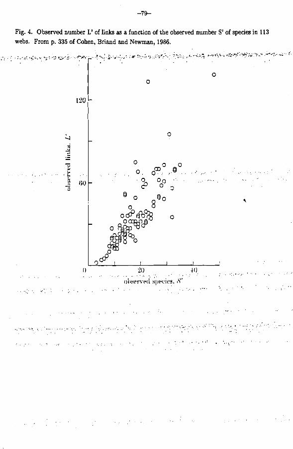
The fifth law is that the ratio of links to species is scale-invariant. This turns out to be fundamental. Fig. 4 plots the observed number of links in each food web against the observed number of species, for 113 webs (Cohen, Briand and Newman, 1986). We find a straight line with slope about 2. That means that a web of 25 species has on average about 50 links. We first came across this generalization with 62 webs (Cohen and Briand, 1984). Then Briand collected an additional 51 webs, and we found (Cohen, Briand and Newman, 1986) that the new data superimpose beautifully on the old data. This scaleinvariant ratio of links to species is a consistent feature of nature, not something we have invented.

In summary, I have reviewed evidence for five "laws" of food webs. Qualitatively, these laws state that cycles are rare, chains are short, and there is scaleinvariance in the proportions of different kinds of species, in the proportions of different kinds of links, and in the ratio of links to species. We have quantified each of these laws. 4. Models L

Let me turn now from empirical regularities to models. Here some mathematics is inevitable. This reminds me of a story.

A mathematician and an ecologist were sharing a cell the night before their execution (for crimes unimaginable). The executioner came in to ask their last wishes.

The mathematician looked over at the ecologist and said, "I've been doing some work in mathematical ecology. I have some interesting results. Before I die, I would like to give a seminar on my work to an ecologist .I1

"Certainly", said the executioner, "we'll arrange it tomorrow morning." He then

turned to the ecologist. "And what would you like?" The ecologist said, "I would like to be executed before the seminar."

Let S denote the number of trophic species and L the number of links. We enumerate all the species along both the rows and columns of a Itpredation matrix," a square table of numbers with S rows and S columns. Name the matrix A. We put a 1 in the intersection of row i and column j if the species labeled j eats the species labeled i, and a 0 otherwise. Since I am excluding cannibalism, all the diagonal elements (where i = j) are 0.

Fig. 2 Three ratios, plotted as a function of the number of species, show scaleinvariance in the proportions of species. The fitted lines are constrained to be horizontal. (a) Top species/total species. The height of the line is 0.2853. (b) Intermediate species/total species.

..:; .,:.,The. height of.the linecis 05251;..:.(c).Basal.species/total .&pedes.. :The height;of thk- line,is?:, . :-...: - .:'';I:' r '

0.1896. From p. 265 of Briand and Gohen, ,1984:

TOTAL SPECIES

Fig. 3. Four ratios, plotted as a function of the number of species, show scaleinvariance in the proportions of links. The fitted lines are constrained to be horizontal. (a) Basal-intermediate links/total links. The height of the line is 0.274. (b) Basal-top links/total links. The height of the line is 0.077. (c) Intermediateintermediate links/total links. The height of the line is 0.301. (d) Intermediatetop links/total links. The height of the line is 0.348. The points in the upper left corner of (a) are based on very few links. From p. 4107 of Cohen and Briand, 1984.

Fig. 4. Observed number L' of links as a function of the observed number S' of species in 113 webs. From p. 335 of Cohen, Briand and Newman, 1986.

+.'-

In terms of this predation matrix, the total number of links is the sum of the elements of A. The sum picks up a 1 if there is a link from prey to predator and a 0 if there is no link.

The predation matrix also tells whether a species is top. If a species is top, then nobody eats it. That means that the row of that species should be all 0's. So a 0-row i corresponds to a top species. Similarly, a O-column corresponds to a basal species because the species is not eating anything. A species that has neither a Grow nor a O-colurnn is intermediate.

I am going to present first a model that does not work. The calculation in this model is simple and gives the flavor of a more complicated model that does work. For the model that does work, I will just describe the results without going through the calculations.

Here is the simplest model I could think of: the anarchy model. I hope you will agree that it has some beautiful features. The anarchy model assumes that the probability that any species j eats any other species i is just CIS, independently of whatever else is going on in the food web. That is a simple model. (The brazen unreality of the assumption that all

. species act by identical and independent random mechanisms is just what lends verisimilitude . to the story about the jailed mathematician and ecologist. But wait and see what emerges from this tissue of fiction!) It follows that the probability that species j

does not eat species i is 1 - CIS. On the average each species eats c species chosen from, among the S possible species, randomly and independently of all other species.

How do the anarchy model's predictions compare with our five laws? The expected number of links is the expectation of the sum of the predation matrix elements. As is conventional, I will use E to denote average or expected number, so E(L) denotes the

2 expected number of links. There are S elements in the predation matrix A and the probability is c/S that an element a.. equals 1. The expected sum of the elements is s2 x

IJ

c/S = cS = E(L). We have to extract the constant of proportionality, i.e., the slope in Figure 4, from the data. We take c = 2. That is the only curve-fitting in this model. Everything else is derived. Thus, the anarchy model predicts that the expected number of links should be proportional to the number of species, as observed. The links-species scaling law fits quantitatively because we made it fit by taking c = 2.

Now I show that the anarchy model predicts qualitatively the scaleinvariance in the proportion of top species, but gets the proportion wrong quantitatively. Since there are S species, the expected number of top species is S times the probability that any one species is a top species. The probability that one species is a top species is the probability that the sum of elements in some row is 0. The row sum is 0 if and only if every elements is 0. So E(T) is S times the probability, raised to the S power, that each row element is zero. The

S probability that a single element is 0 is 1 - CIS. As S gets big, (1 - CIS) approaches e*. So E(T)/S, the expected fraction of top species, is asymptotically (for large S) e*. Qualitatively, this is good. It means that as the number of species increases the fraction of

top species does not change (more accurately, the fraction approache3 a limit). This simple model predicts scale-invariance of species proportions.

However, if c = 2 in this formula, e* N 14 percent. The species scaling law is

qualitatively good but quantitatively poor, beguse 14 percent, is too.,pn$l-it.,is not~.nftar the . . . .,.:. .:,.. .. . + . _ . A , . . . . . . . . . . . . ,

one-quarter (iet aldne 29 percedt ) shown in Figure 2. What else does this model predict? The probability that a web has at least one

2 2 y c l e as S goes to infinity is 1 - e* 12. If c = 2, the model predicts that 86 percent of webs should have one or more 2-qcles. That is not good because we found 2-cycles in only 3 of 113 webs.

The principal problems with the anarchy model are that it predicts too many cycles

and that it fails to predict the proportion of top species. Let's fix one problem at a time and see whether that solves any other problems as well. We get rid of the problem with cycles by fiat in the next model, the cascade model.

I am now going to describe the cascade model, but not the calculations required to squeeze results out of it. Assume S species. Somehow nature numbers them from 1 to S (without showing us the numbering). Any species . j in this hierarchy or cascade can feed on . .. . & species i with a lower number i < j (which does not mean that. j &.feed on i, only that j can feed on i). However, species j cannot feed on any'species with a number k at

least as large, k 2 j. The cascade model assumes that each species actually eats any,species below it with some probability d/S, independently of whatever else is going on in the web.

(I have changed notation for the probability parameter from c to d so as not to mix up the. anarchy and cascade models.)

In the predation matrix A, a.. is 0 always if i 2 j. The predation matrix with this 1J

labelling is strictly upper triangular. An element above the diagonal (i < j) is 1 with probability d/S and is 0 with probability 1- d/S, and all elements are independent.

To derive predictions from the cascade model, we must take one number from nature. To simplify slightly, we estimate d approximately as twice the observed number of links ' divided by the observed number of species; .we multiply the number of links by two here because roughly half of the matrix is empty. As the number of species becomes large, the cascade model predicts 26 percent top species, 48 percent intermediate species and 26 percent

basal species. We observed 29 percent top species, 53 percent intermediate and 19 percent basal. We predict the following percentages of basal-intermediate, basal-top, . . . intermediate-intermediate and intermediate-top links: 27, 13, 33 and 27. We observed,

correspondingly, 27, 8, 30 and 35. I think it is nice that the cascade model reproduces all the laws of scale-invariance

qualitatively, but far more striking that the cascade model gives a remarkable quantitative agreement between observed and predicted proportions. We put one number d into the cascade model and get out five independent numbers (because the three species proportions

have to add up to 1 and the four link proportions have tc:~ add up to 1). I would like to emphasize that these predictions use only the observed ratio of links to species.

For a finite number of species, we calculated from the cascade model the expected fraction of top species and the predicted variance. Figure 5 shows that the cascade model predicts not only the means but also the variability in the proportion of top species. We do not know whether the cascade model can predict the variability in proportions of links because we do not know how to calculate analytically what variability the cascade model predicts.

The cascade model was built to, and does, explain qualitatively and quantitatively the mean proportions of different kinds of species and links. Can the cascade model describe the number of chains of each length counting all the possible routes from a basal species to a top species?

Let me illustrate with an artificial example (Figure 6) how to get a frequency histogram of chain length from a food web. The link from 1 to 2 is a chain of length 1. The path 1, 3, 4 is a chain of length 2, and the path 1, 3, 5 is another chain of length 2. A numerical summary of the chain length distribution of the web in Figure 6 is that it has40ne chain of length 1, two chains of length 2 and no longer chains.

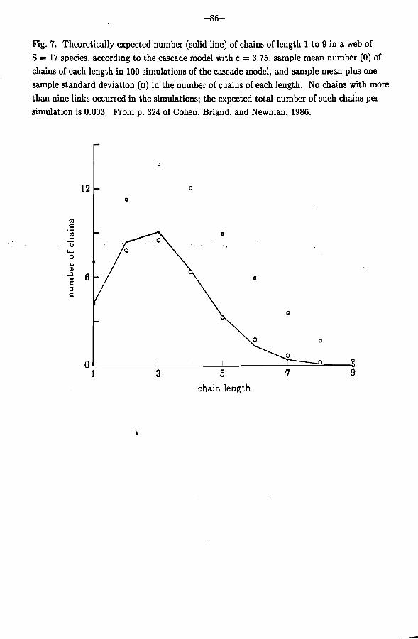
Figure 7 shows the expected number of chains of each length, according to the cascade model, using parameters of a typical web, namely 17 species and d close to 4. Figure 7 also shows the results of one hundred computer simulations of the model using the same parameters. The sample mean numbers of chains of each length agree well with theoretically expected number calculated from the model. That agreement increases the probability that both the calculations and the simulations are right.

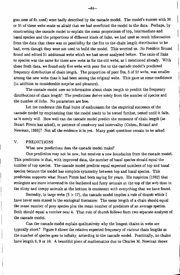
To see how well the cascade model predicts the observed distribution of chain length of a given real web, we generated random webs according to the cascade model with the parameters of the observed web. We measured how often the chain length distribution of a random web was further from the chain length distribution predicted by the cascade model than the real observed chain length distribution was from the predicted distribution. We used two measures of goodness of fit: the sum of squares of differences and a measure like Pearson's chi-squared. If the discrepancy between the observed and the expected frequency distributions was smaller than most of the discrepancies between webs randomly generated

according to the cascade model and the mean frequency distribution expected from the model, we said the fit was good. If the discrepancy between observed and

simulation is 0.003. From p. 324 of Cohen, Briand, and Newman, 1986. predicted chain length distributions was bigger than most simulated discrepancies, we said the fit was bad.

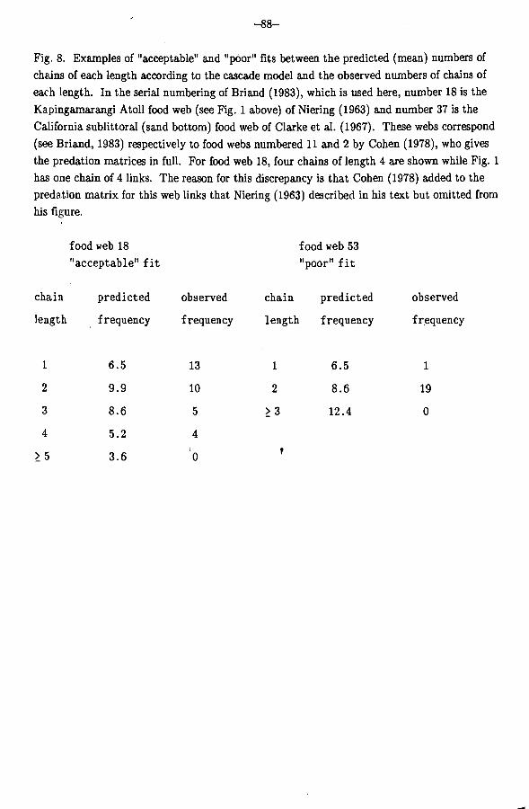
Have no illusions about what a good fit means. Food web 18 in Figure 8 illustrates a good fit. Food web 53 illustrates a poor fit.

Of 62 webs in Briand's original collection, 11 or 12 (depending on the measure of

Fig. 5. The predicted mean pr~pclrtion of top species (middle line) and a confidence interval + of -2 standard deviations (upper and lower lines) as a function of total species S, according to the cascade model. X is constant environment, o is fluctuating environment. The

:symbols. . , X,, and ?: o . . : ... have : ...... .a%:,,, . been,pert.urbed . . . . from their ... exact ...... locations . . . by a small random amo.unt .... .... . . .... ..,-- b . > , :: ..* * a * L... .-:-< <. ; :.:.,, ..-;,: * - .-.-:.. ,:.!' "' . . to indicate when se;eral food'kebs.have exactly the s h e coordinate. ' The data &i replotted from Briand and Cohen, 1984. From p. 436 of Cohen and Newrnan, 1985.

goo(-ness of fit used) were badly described by the cascade model. The model's success with 50 or 51 of these webs made us afraid that we had overfitted the model to the data. Perhaps, by constructing the cascade model to explain the mean proportions of top, intermediate and basal species and the proportions of different kinds of links, we had used so much information from the data that there was no possibility for the fits to the chain length distribution to be bad, even though they were not used to build the model. This worried us. So FrCdCric Briand found and edited 51 additional webs which we had never analyzed before. The ratio of links to species was the same for these new webs as for the old webs, as I mentioned already, With these fresh data, we found only five webs with poor fits to the cascade model's predicted frequency distribution of chain length. The proportion of poor fits, 5 of 51 webs, was smaller among the new webs than it had been among the original webs. This gave us some confidence (in addition to considerable surprise and pleasure).

The cascade model uses no information about chain length to predict the frequency distributions of chain length! The predictions derive solely from the number of species and the number of links. No parameters are free.

Let me moderate this final burst of enthusiasm for the empirical successes of the cascade model by emphasizing that the model needs to be tested further, tested until it fails, as it surely will. How well can the cascade model predict the moments of chain length (as Stuart Pimrn has asked), or patterns of omnlvory and internality (Cohen, Briand and Newman, 1986)? Not all the evidence is in yet. Many good questions remain to be asked.

V. PREDICTIONS What new predictions does the cascade model make?

One prediction may not be new, but receives a new foundation from the cascade model. This prediction is that, with improved data, the number of basal species should equal the number of top species. The cascade model predicts equal expected numbers of top and basal species because the model has complete symmetry between top and basal species. This prediction supports what Stuart Pimm had been saying for years. His suspicion (1982) that ecologists are more interested in the feathered and furry animals at the top of the web than in the slimy and creepy animals at the bottom is consistent with everything that we have found.

Secondly, in large webs (S > 17), the cascade model implies a rule of thumb which I have never seen stated in the ecological literature: The mean length of a chain should equal the mean number of prey species plus the mean number of predators of an average species. Both should equal a number near 4. That rule of thumb follows from two separate analyses of the cascade model.

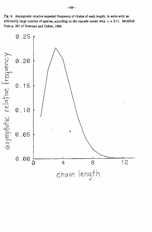
Can the cascade model explain qualitatively why the longest chains in webs are typically short? Figure 9 shows the relative expected frequency of various chain lengths as the number of species goes to infinity, according to the cascade model. Practically, no chains have length 8, 9 or 10. A beautiful piece of mathematics due to Charles M. Newman shows

Fig. 6 I'lypothetical food web to illustrate how the frequency distribution of chain lengths is counted. There is one chain of length 1 (from species 1 to species 2) and there are two chains of length 2 (from species 1 to species 4 and from species 1 to species 5).

. .

Fig. 7. Theoretically expected number (solid line) of chains of length 1 to 9 in a web of S = 17 species, according to the cascade model with c = 3.75, sample mean number (0) of chains of each length in 100 simulations of the cascade model, and sample mean plus one sample standard deviation (o) in the number of chains of each length. No chains with more than nine links occurred in the simulations; the expected totail number of such chains per simulation is 0.003. From p. 324 of Cohen, Briand, and Newman, 1986.

chain length

that, in very large webs, the longest chain grows like log S/log log S. That is very slow growth. In a web with 1018 species, which is probably an upper bound for the world, the cascade model predicts that the longest chain will almost never have more than 20 links.

VI. APPLICATIONS What good is all this for the real world of practical affairs? Let me speculate about

four ways this work may contribute to human well-being. First, environmental toxins cumulate along food chains. An understanding of the

distribution of the length of food chains is essential, though not sufficient, for understanding how toxins are concentrated by living organisms.

Second, an understanding of the invariant properties of food webs is essential for anticipating the consequences of species' removals and introductions. Such perturbations of natural ecosystems are being practiced with increasing frequency in programs of biological control. So far, people have not been very successful at anticipating all the consequences of introducing or eliminating species. An understanding of food webs should help anticipate the consequences.

Third, an understanding of food webs will help in the design of nature reserves and of those future, mobile nature reserves that will be required for long-term manned spaceflight. A nature reserve with all top species would be expected to have trouble, according to the cascade model. For humans to survive and to be fed in space, we need to know more about the care and feeding of food webs.

Fourth, and finally, since food webs include man, perhaps an understanding of such t webs will give us a better understanding of man s place in nature, here on earth. It is a

remarkable fact that we have not detected any consistent pattern of difference between those webs in which man is a species and those webs in which man is not a species.

Of course, as a graduate student pointed out to me when I said this, we have not looked yet at agricultural ecosystems strongly influenced by man. When we look at a new class of food webs, we might see new patterns. God created graduate students to keep us all honest.

Fig. 8. Examples of "acceptable" and "poor" fits between the predicted (mean) numbers of chains of each length according to the cascade model and the observed numbers of chains of each length. In the serial numbering of Briand (1983), which is used here, number 18 is the

Kapingamarangi Atoll food web (see Fig. 1 above) of Niering (1963) and number 37 is the California sublittoral (sand bottom) food web of Clarke et al. (1967). These webs correspond (see Briand, 1983) respectively to food webs numbered 11 and 2 by Cohen (1978), who gives the predation matrices in full. For food web 18, four chains of length 4 are shown while Fig. 1 has one chain of 4 links. The reason for this discrepancy is that Cohen (1978) added to the predation matrix for this web links that Niering (1963) described in his text but omitted from his figure.

food web 18 "acceptablett f i t

food web 53 llpoor" f i t

chain predicted observed chain predicted observed

length frequency frequency length frequency frequency

Fig. 9. Asymptotic relative expected frequency of chains of each length, in webs with an arbitrarily large number of species, according to the cascade model with c = 3.71. Modified from p. 361 of Newrnan and Cohen, 1986.

Acknowledgements

This work was supported in part by U.S. National Science Foundation grant BSR 4-07461, a Fellowship to J.E.C. from the John D. and Catherine T. MacArthur Foundation, and the hospitality of Mr. and Mrs. William T. Golden. Charles M. Newman and Stuart Pimm made numerous corrections and improvements to a previous draft.

REFERENCES

Briand, F. 1983 Environmental control of food web structure. Ecology 64, 253-263. Briand, F. and Cohen, J. E. 1984 Community food webs have scale-invariant structure,

Nature 307, 264-266. '-

Clarke, T.A., Flechsig, A.O., and Grigg, R.W. 1967 Ecological studies during Project Sea Lab 11. Science 157, 1381-1389.

Cohen, J . E. 1977 Ratio of prey to predators in community food webs. Nature 270, 165-167.

Cohen, J. E. 1978 Food Webs and Niche S~ace. Princeton: Princeton University Press, 189 pp.

Cohen, J. E. and Briand, F. 1984 Trophic links of community food webs. Proc. Nat. Acad. Sci. U.S.A. 81, 41054109.

Cohen, J. E., Briand, F., and Newman, C. M. 1986 A stochastic theory of community food webs. 111. Predicted and observed lengths of food chains. Proc. Rov. Soc. (London) B 228, 317-353. m

Cohen, J. E., and Newman, C. M. 1985 A stochastic theory of community food webs. I. Models and aggregated data. P r o c . 1 B 224,421-448.

Cohen, J. E., Newman, C. M. and Briand, F. 1985 A stochastic theory of community food webs. I. Models and aggregated data. Proc. Rov. Soc. (London1 B 224,421-448.

Cohen, J. E., Newman, C. M. and Briand, F. 1985 A stochastic theory of community food webs. 11. Individual webs. Proc. Roy. Soc. (London) B 224, 449461.

DeAngelis, D. L., Post, W. M. and Sugihara, G. (4s .) 1983 Current Trends in Food Web Theory. ORNL-5983. Oak Ridge, Tennessee: Oak Ridge National Laboratory.

Diamond, J. M. and Case, T. J. (4s .) 1985 Communitv Ecolo~v. Cambridge: Harper and Row. 665 pp.

Hutchinson, G. E. 1959 Homage to Santa Rosalia or why are there so many kinds of animals? American Naturalist 93, 145-159.

Kikkawa, J. and Anderson, D.J. (eds.) 1986 Communitv Ecolo~v: Pattern and Process. Melbourne and Oxford: Blackwell Scientific. 432 pp.

Newman, C. M. and Cohen, J. E. 1986 A stochastic theory of community food webs. IV.

Theory of food chain lengths in large webs. Proc. Rov. Soc. (London) B 228,355-377. Niering, W. A. 1963 Terrestrial ecology of Kapingamarangi Atoll, Caroline Islands.

Ecological Mono~ra~hg 33, 131-160. Pimm, S. 1982 Food Webs. London: Chapman and Hall. 219 pp. Pimm, S.L. In press, The geometry of niches. This volume, Chapter 7.

Sugihara, G. 1984 Graph theory, homology, ~d food webs. Proc. Svmv. Av~lied Math.

30, 83-101. Providence, RI: American Mathematical Society.