Linking CGE and Microsimulation Models: A Comparison of ... · Linking CGE and Microsimulation...

INTERNATIONAL JOURNAL OF MICROSIMULATION (2010) 3(1) 72-91

Linking CGE and Microsimulation Models: A Comparison of

Different Approaches Giulia Colombo Department of Economic and Social Science - Catholic University of Milan and SiNSYS NV/SA; e-mail: [email protected]

ABSTRACT: In the literature that studies income inequality and poverty, a recent development has been the development of models that link together a macroeconomic model (usually a Computable General Equilibrium (CGE) model) and a microsimulation model. Linking the two types of model allows the modeller to take into account full agents‟ heterogeneity, whilst at the same time considering the general equilibrium effects of a proposed policy reform. In this paper, I first review in detail three approaches to building linked CGE-microsimulation models: one in accordance with the fully integrated approach, and two following the layered approach (the so-called Top-Down and Top-Down/Bottom-Up approaches). The

principal goal of the paper is to present a considered evaluation of the merits and demerits of these alternative methods currently used to link CGE and microsimulation models. To do so I use all three approaches to model the macro- and micro-economic impacts of a policy shock to an archetypical economy (constructed using fictitious data), and compare the results. This analysis highlights the importance of (i) consistency between the underlying macro- and micro-data; and (ii) the precise

mechanisms by which feedback effects are passed between the macro and micro models. I develop this

latter point further by detailed analysis of the TD/BU approach outlined by Savard (2003), leading to a proposed refinement in the way that feedback effects from the micro level of analysis are incorporated back into the CGE model. 1. INTRODUCTION

The study of poverty and inequality in developing countries usually requires two main focuses: on one side a microeconomic focus is required to have a detailed and precise picture of incomes and/or expenditures at the individual and household level, and to model individual and household behavioural responses to some

reforms/shocks, with a special concern for those whose income is around the poverty line; on the other side, a macroeconomic focus is often

needed, as most of the economic policies (structural adjustment programs or trade liberalizations, for example) and of the exogenous

shocks commonly analyzed for developing countries (such as fluctuations in the world price of raw materials and agricultural exports) are often macroeconomic phenomena (or may have, at least, some structural effects on the economy). Since the pioneering work by Adelman and

Robinson (1978) for South Korea and Lysy and Taylor (1980) for Brazil, many Computable General Equilibrium (CGE) models for developing countries combine a highly disaggregated representation of the economy within a consistent macroeconomic framework and a description of the distribution of income through a small number

of representative households (RHs). In order to account for heterogeneity among the main sources of the changes in household income, several “representative households” are necessary. Despite this need for variety, the number of RHs is generally small in these models

(usually less than 10). The CGE/RH framework sometimes explicitly considers that households within a RH group are heterogeneous in a “constant” way. That is, in order to capture within-group inequality, it is assumed that the distribution of relative income

within each RH follows an exogenous statistical law1. But the assumption that relative incomes are

constant within household groups is not reflected in reality. Indeed, empirical analyses conducted on household surveys show that the within-group component of observed changes in income distribution is generally at least as important as the between-group component of these changes2. Thus, the RH approach based on this assumption

may be misleading in several circumstances, and this is especially true when studying poverty. This argument may be better understood by presenting

an example: consider a shock on the world market of a certain good, which leads to a decrease in the exports and to a domestic contraction of this

sector in the specific exporting country under study. After the simulation of the shock with a CGE/RH model, suppose that I find a little change in the mean income of a particular RH group, say workers in the agricultural sector. In this case, poverty might be increasing by much more than suggested by this drop in income: indeed, in some

households there may be individuals that lose their job after the shock, or that encounter more difficulties in diversifying their activity or consumption than others. For these individuals or families, the relative fall in income is necessarily larger than for the whole group, and this fall in their income is not represented by the slight fall in

the mean income of the whole group. Suppose, moreover, that the initial income of these individual was low. Then poverty may be increasing by much more than what predicted by a simple RH model, which is based on the assumption of distribution neutral shocks. So, the

RH approach does not capture the effects that a shock or a policy change may have on single individuals or households within a RH group. In contrast, microsimulation models can be very precise and detailed in their representation of microeconomic individual behaviour, but

COLOMBO Linking CGE and microsimulation models: a comparison of different approaches 73

necessarily miss an important part of the story

since they involve only a partial equilibrium analysis. In short, they miss a very important

aspect represented by general equilibrium models which is the structural effects of the reform/shock under study.

In order to overcome these problems, the recent literature has tried to develop new modelling tools which should be able at the same time to account for heterogeneity and for the possible general equilibrium effects of the policy reform (or the exogenous shock) under study. In view of the fact that most of the available economic models have

either a microeconomic or a macroeconomic focus, and hence do not address the question adequately, the recent literature has focused on the possibility of combining two different types of models. In particular, some authors have tried to link microsimulation models to CGE models, in

order to account simultaneously for structural

changes, for general equilibrium effects of the economic policies, and for their impacts on households‟ welfare, income distribution and poverty. (More generally, this current of the literature develops the use of micro-data drawn from household surveys in the context of a

general equilibrium setting, which is usually but not necessarily a CGE model.) The literature that follows this approach has flourished in recent years: there are, among others, the important contributions by Decaluwé et al. (1999a) and (1999b), Cogneau and Robilliard (2001, 2004 and 2006), Cockburn (2001), Cogneau (2001),

Bourguignon et al. (2003b), Boccanfuso et al. (2003), Savard (2003) and Davies (2009). In this paper I have two main aims. First, to

summarise recent developments in this field by detailing the three main methods developed to link the micro-data from a survey into a CGE

model: the full integration of survey data into a CGE framework, as is done for instance in Cockburn (2001); the linking of a behavioural microsimulation model to a CGE through a set of specific equations as developed in Bourguignon et al. (2003b) – the so called Top-Down method; and

the iterative coupling of CGE and microsimulation outputs as developed by Savard (2003) – the Top-Down/Bottom-Up model. Second, to present an assessment of the relative strengths and weaknesses of each of these three approaches. To fulfil these aims, in this paper I first outline

each approach to linking CGE and microsimulation

models in detail (Sections 2 to 4). I then use all three approaches to simulate the impact of an identical policy reform, using as inputs for each the same data from a fictitious economy. The use of fictitious data describing a simple economy permits better understanding of the differences

that are observed in the results of the models, and of the causes that generate them. Having constructed and run the models, in Section 5 I compare and contrast the macro- and micro-economic outcomes derived from each type of model linking, drawing lessons regarding the

importance of data consistency and feedback

mechanism. This leads on to a more detailed analysis of the TD/BU approach as developed by

Savard (2003), and the proposal of an alternative way of taking into account feedback effects from the micro level of analysis into the CGE model.

2. THE INTEGRATED APPROACH The first approach to linking CGE and microsimulation models that I will consider is the „integrated‟ approach. The main intuition behind this approach is to substitute the Representative

Household Groups inside a standard CGE model with the real households that are found in the survey. The first attempt in this direction was made by Decaluwé et al. (1999b). Among the models following this approach there are the works by Cockburn (2001) for Nepal, by

Boccanfuso et al. (2003) for Senegal, and by

Cororaton and Cockburn (2005), who studied the case of the Philippine economy. In practice, under this approach, one passes from a model with, for instance, ten representative agents to a model with thousands of agents, thus

increasing the computational effort, but leaving substantially unchanged the modelling hypothesis of a standard CGE model. Basically this approach does not include a true microsimulation module in the modelling framework, but tries to incorporate the data from the household survey into the CGE model.

The first step in building such a model is to pass from the representative households‟ data to population values; to do this, one should weight

each variable at the household level with the weights given in the survey, thus obtaining population values for each variable. After this, a

procedure is required to reconcile these population data coming from the survey (incomes and expenditures) with the accounts contained in the social accounting matrix (SAM). (For a fuller account of the SAM, see Section 3.2.) The literature on data reconciliation offers different

alternatives. One may choose to keep fixed the structure of the SAM and adjust the household survey, or to adjust the SAM in order to meet the totals of the household survey. Intermediate approaches are also possible. Whatever the method used, however, one necessarily loses the structure of the original data, which is one of the

main drawbacks of the integrated approach. For

this paper I have chosen the first alternative, and kept the original composition of households‟ incomes and expenditures unchanged. After these changes in the SAM, one encounters the problem of re-balancing it (row totals must be

equal to column totals). To do this, I used an appropriate program that minimizes least squares3. The CGE model I use for application of the integrated approach is the one described in


Section 3.2, except for the addition of an index

which refers to households. This way, for instance, the consumption demand function in Table 8

becomes:

mmqmqq CBUDHCP ,

where m is now the index for households. One thing should be noted at this point: certain types of equations that are commonly included in

a behavioural model, such as occupational choice equations, are not easily modelled within standard CGE modelling software (see Savard, 2003), so that CGE-MS models that follow the fully integrated approach are not always able to capture the behavioural responses of the agents to the policy reforms that are implemented.

Instead, micro-econometric behavioural modelling provides much more flexibility in terms of the

modelling structure used, and is more suitable to describe the complexity of household and individual behaviour, and the way this may be affected by the changes in the macroeconomic framework that are subsequent to a policy reform

or an external shock. The main point here is that with a CGE model like the one used for the integrated approach I am not able to predict which particular individual will enjoy the reduction (or will suffer from the rise) in

the employment level on the basis of some characteristics of the individual or of the household that can be observed; this instead can be done through a behavioural microsimulation model. Indeed, the main feature that differentiates a

microsimulation model from a standard CGE framework (not only one with representative agents, but even one with thousands of households from a survey, as we have seen) is that it works at the individual level, selecting those individuals, on the basis of their personal or family characteristics, that show the highest

probability of changing their labour market status. This fact could bring about significant differences in the results between the two types of models,

even after the same policy simulation, as we will

see below.

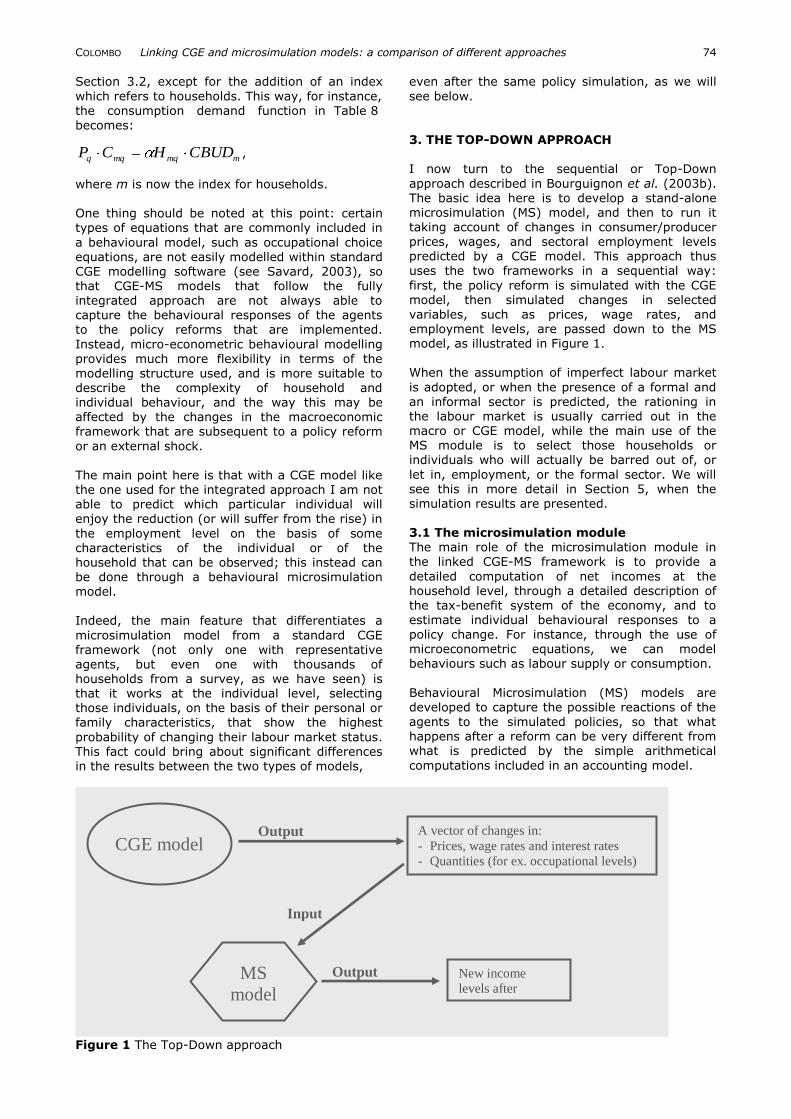
3. THE TOP-DOWN APPROACH I now turn to the sequential or Top-Down

approach described in Bourguignon et al. (2003b). The basic idea here is to develop a stand-alone microsimulation (MS) model, and then to run it taking account of changes in consumer/producer prices, wages, and sectoral employment levels predicted by a CGE model. This approach thus uses the two frameworks in a sequential way:

first, the policy reform is simulated with the CGE model, then simulated changes in selected variables, such as prices, wage rates, and employment levels, are passed down to the MS model, as illustrated in Figure 1.

When the assumption of imperfect labour market

is adopted, or when the presence of a formal and an informal sector is predicted, the rationing in the labour market is usually carried out in the macro or CGE model, while the main use of the MS module is to select those households or individuals who will actually be barred out of, or

let in, employment, or the formal sector. We will see this in more detail in Section 5, when the simulation results are presented. 3.1 The microsimulation module The main role of the microsimulation module in the linked CGE-MS framework is to provide a

detailed computation of net incomes at the household level, through a detailed description of the tax-benefit system of the economy, and to estimate individual behavioural responses to a

policy change. For instance, through the use of microeconometric equations, we can model behaviours such as labour supply or consumption.

Behavioural Microsimulation (MS) models are developed to capture the possible reactions of the agents to the simulated policies, so that what happens after a reform can be very different from what is predicted by the simple arithmetical

computations included in an accounting model.

Figure 1 The Top-Down approach

CGE model

Input

A vector of changes in:

- Prices, wage rates and interest rates

- Quantities (for ex. occupational levels)

MS

model

New income

levels after

simulation

Output

Output


In this section I will describe in detail a simple

behavioural model, following quite closely the discrete labour supply choice model used in

Bourguignon et al. (2003b). Another description of a similar MS model for labour supply can be found in Bussolo and Lay (2003) with their model for Colombia, and in Hérault (2005), who built a

model for the South African economy. For the building of the model I will use fictitious data describing a very simple economy. In the household survey I have information about some individual characteristics, such as age, sex, level of qualification, education, labour and capital

income, the eventual receipt of public transfers, and the activity status. For the sake of simplicity, I have stated that each individual at working age (16-64) can choose between only two alternatives: being a full-time wage worker, or being unoccupied. There are other variables in the

survey that refer to households rather than to

individuals, for example the area of residence, the number of adults (over 18 years old) and children (under 18), and so on. Also for the sake of simplification, I have grouped all consumption goods within the economy into two main categories.

The focus of my distribution and poverty analysis will be on disposable income, even if in principle an inequality and poverty analysis could also be conducted on expenditure rather than on income levels.

I derive income variables referring to households from initial individual data by summing up individual values for each household member; this way, I obtain households‟ labour and capital

incomes, households‟ public transfers and households‟ total income, respectively:

mNC

imim YLYL

1

mNC

imim YKYK

1

mNC

imim TFTF

1

mmmm TFYKYLY ,

where YLmi is labour income of individual i

member of household m, YKmi his/her capital income, and TFmi are the public transfers he/she receives from government. All these quantities are summed up for each family over all the individuals

belonging to the family (NCm is the number of components of household m); then, household m‟s total income, Ym, is the sum of all incomes received by the family: labour income, capital income, and public transfers. For the benchmark situation, I assume all initial

prices normalized at one.

3.1.1 The model

The core of the behavioural model is represented by the following two equations:

mimimimi vcXbaYLLog )( (1)

]0[ mimimimi RWZIndW (2)

The first equation is a regression model for log-wage earnings, while the second one represents individuals‟ “choice” for labour market status (see below for further explanations). The rest of the MS module comprises simple

arithmetical computations of price indices, incomes, savings and consumption levels. As the parameters entering the following equations (marginal propensity to save mpsm, income tax rates γ, and budget shares ηmq) are constant, this

part of the model may be regarded as purely accounting, as it does not contain any possible

behavioural response to policy simulations. Household m‟s income generation model:

mm

NC

imimim TFYKWYLY

m

1

(3)

Household disposable (after tax) income:

mm YYD )1( (4)

Household specific consumer price index:

2

1qqmqm PCPI (5)

Real disposable income:

mmm CPIYDYDR / (6)

Savings:

mmm YDmpsS

(7)

Household consumption budget:

mmm SYDCEBUD

(8)

Consumption expenditure for commodity q:

mmqmq CEBUDCE (9)

Consumption level of commodity q:

q

mqmq

P

CEC (10)

Household m‟s capital income:

mm KSPKYK (11)

See Table 1 for a description of the subscripts.


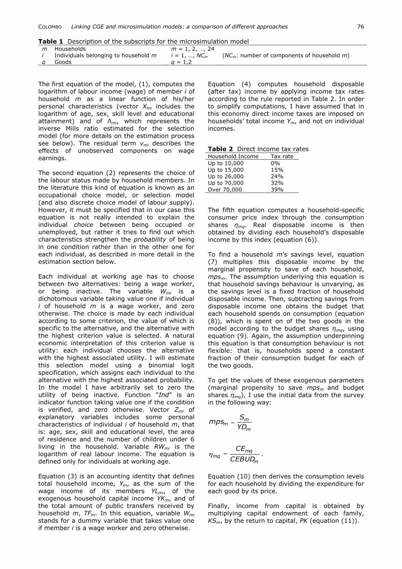
Table 1 Description of the subscripts for the microsimulation model m Households m = 1, 2, …, 24 i Individuals belonging to household m i = 1, …, NCm (NCm: number of components of household m) q Goods q = 1,2

The first equation of the model, (1), computes the logarithm of labour income (wage) of member i of

household m as a linear function of his/her personal characteristics (vector Xmi

includes the

logarithm of age, sex, skill level and educational attainment) and of Λmi, which represents the inverse Mills ratio estimated for the selection model (for more details on the estimation process

see below). The residual term vmi describes the effects of unobserved components on wage earnings. The second equation (2) represents the choice of the labour status made by household members. In the literature this kind of equation is known as an

occupational choice model, or selection model (and also discrete choice model of labour supply). However, it must be specified that in our case this equation is not really intended to explain the individual choice between being occupied or unemployed, but rather it tries to find out which characteristics strengthen the probability of being

in one condition rather than in the other one for each individual, as described in more detail in the estimation section below. Each individual at working age has to choose between two alternatives: being a wage worker,

or being inactive. The variable Wmi is a dichotomous variable taking value one if individual i of household m is a wage worker, and zero otherwise. The choice is made by each individual

according to some criterion, the value of which is specific to the alternative, and the alternative with the highest criterion value is selected. A natural

economic interpretation of this criterion value is utility: each individual chooses the alternative with the highest associated utility. I will estimate this selection model using a binomial logit specification, which assigns each individual to the alternative with the highest associated probability. In the model I have arbitrarily set to zero the

utility of being inactive. Function “Ind” is an indicator function taking value one if the condition is verified, and zero otherwise. Vector Zmi of explanatory variables includes some personal characteristics of individual i of household m, that is: age, sex, skill and educational level, the area

of residence and the number of children under 6

living in the household. Variable RWmi is the logarithm of real labour income. The equation is defined only for individuals at working age. Equation (3) is an accounting identity that defines total household income, Ym, as the sum of the

wage income of its members YLmi, of the exogenous household capital income YKm, and of the total amount of public transfers received by household m, TFm. In this equation, variable Wmi stands for a dummy variable that takes value one if member i is a wage worker and zero otherwise.

Equation (4) computes household disposable (after tax) income by applying income tax rates

according to the rule reported in Table 2. In order to simplify computations, I have assumed that in this economy direct income taxes are imposed on households‟ total income Ym, and not on individual incomes.

Table 2 Direct income tax rates Household Income Tax rate

Up to 10,000 0% Up to 15,000 15% Up to 26,000 24% Up to 70,000 32% Over 70,000 39%

The fifth equation computes a household-specific consumer price index through the consumption

shares ηmq. Real disposable income is then obtained by dividing each household‟s disposable income by this index (equation (6)). To find a household m‟s savings level, equation (7) multiplies this disposable income by the marginal propensity to save of each household,

mpsm. The assumption underlying this equation is that household savings behaviour is unvarying, as the savings level is a fixed fraction of household disposable income. Then, subtracting savings from disposable income one obtains the budget that each household spends on consumption (equation

(8)), which is spent on of the two goods in the model according to the budget shares ηmq, using

equation (9). Again, the assumption underpinning this equation is that consumption behaviour is not flexible: that is, households spend a constant fraction of their consumption budget for each of the two goods.

To get the values of these exogenous parameters (marginal propensity to save mpsm and budget shares ηmq), I use the initial data from the survey in the following way:

m

mm

YD

Smps

m

mqmq

CEBUD

CE.

Equation (10) then derives the consumption levels for each household by dividing the expenditure for each good by its price. Finally, income from capital is obtained by multiplying capital endowment of each family, KSm, by the return to capital, PK (equation (11)).


The initial values of the variables Cmq and KSm

(consumption levels and capital endowments, respectively) are derived from the survey data

making use of the assumption that in the benchmark situation all prices and returns are equal to one:

mqmq CEC (12)

mm YKKS (13)

Moreover, I assume that public transfers paid to households and household capital endowments

are exogenously given. They are fixed at the level reported in the survey, for public transfers, and at the level as computed in equation (13), for capital endowment, respectively. 3.1.2 Estimation of the model

The only two equations in the MS module that need to be estimated are equations (1) and (2). The former, which expresses the logarithm of wage earnings as a linear function of some individual characteristics and of Λmi, the inverse Mills ratio, was estimated using a Heckman two-step model (see Heckman (1976) and (1979)). I

followed this approach to correct for the selection bias which is implicit in a wage regression, that is, the fact that I observe a positive wage only for those individuals that are actually employed at the moment of the survey. The results of the estimation are reported in Table

3. The estimation was conducted on the sub-

sample of individuals at working age (16-64). The aim of the wage equation in the model is to assign

an estimated wage to the individuals that are inactive in the survey, and change their labour market status after the simulation run.

Parameters of equation (2) were obtained through the Maximum Likelihood estimation using a binomial logit model and assuming that the residual terms εi are distributed according to the Extreme Value Distribution – Type I4. The estimation was conducted on the sub-sample of individuals at working age (16-64). Explanatory

variables include individual characteristics such as the logarithm of predicted real wage, sex, skill and education level, as well as the region of residence and a variable accounting for the presence or not of children under 6 years old in the household. Results are presented in Table 4.

With the estimated coefficients I cannot perfectly predict the true labour market statuses that are actually observed in the survey. Thus, following the procedure described in Duncan and Weeks (1998), I drew a set of error terms εi for each individual from the extreme value distribution, in

order to obtain an estimate that is consistent with the observed activity or inactivity choices. From these drawn values, I select 100 error terms for each individual, in such a way that, when adding it to the deterministic part of the model, it perfectly predicts the activity status that is observed in the survey. In other words, the residual term for an

Table 3 Heckman selection model, two-step estimates Coefficient Std. Error z P>|z|

constant 7.0321 0.3145 22.36 0.000 ln(age) 0.6978 0.0833 8.38 0.000 sex -0.4662 0.1018 -4.58 0.000 qualification 0.3966 0.0772 5.14 0.000 education 0.5250 0.0872 6.02 0.000

Mills ratio 0.2160 0.1473 1.47 0.143 Selection ln(age) 0.3386 0.0807 4.19 0.000 sex -1.5492 0.2803 -5.53 0.000 qualification 1.0204 0.2729 3.74 0.000 children under 6 0.1682 0.2368 0.71 0.478 region -0.7515 0.2980 -2.52 0.012

rho 0.7628 sigma 0.2832

Dependent variable: logarithm of wage

Table 4 Binary logit model of labour status choice Coefficient Std. Error z P>|z|

ln(real wage) 0.1972 0.0465 4.25 0.000 sex -1.8948 0.4078 -4.65 0.000 qualification 1.4408 0.4257 3.38 0.001 region -0.7185 0.3295 -2.18 0.029 children under 6 0.2691 0.2973 0.91 0.365 education -0.7633 0.6717 -1.14 0.256 Mean dependent var 0.6647 S.D. dependent var 0.4735 S.E. of regression 0.3767 Akaike info criterion 0.9015 Sum squared resid 23.2688 Schwarz criterion 1.0122 Log likelihood -70.6305 Hannan-Quinn criter. 0.9464 Avg. log likelihood -0.4155

Dependent Variable: Activity Status


individual that is observed to be a wage earner in

the survey should be such that:

,0ˆ6ˆˆ

ˆˆ)(ˆˆ

654

321

mimimim

mimimi

SCHCHAREA

QSEXRWLog

while, for an individual that is observed to be inactive in the survey, the same inequality should be of opposite sign (≤).

After a policy change, only the deterministic part of the model is recomputed. Then, by adding the random error terms previously drawn to the recomputed deterministic component, a probability distribution over the two alternatives (being a wage worker or being inactive) is

generated for each individual. This implies that the model does not assign every individual from

the sample to one particular choice, but it gives the individual probabilities of being in one condition rather than in the other. This way, the model does not identify a particular choice for each individual after the policy change, but

generates a probability distribution over the different alternatives. This procedure is also described in Creedy and Kalb (2005); see also Creedy et al. (2002b). 3.2. The CGE model

CGE models are a class of economic models that use economic data to estimate how an economy might react to changes in policy, technology or other external factors. A CGE model consists of a system of equations describing model variables and a database consistent with the model equations. General Equilibrium models are used to

estimate what is the effect of a change in one part of the economy upon the rest. CGE models have been used widely to analyse trade policy. More recently, CGE has become a popular way to estimate the economic effects of measures to reduce greenhouse gas emissions.

CGE models always contain more variables than equations, so that some variables must be set outside the model. These variables are usually called exogenous variables. The choice of which variables are to be exogenous is called the model closure. Variables defining technology, consumer

tastes, and government instruments (such as tax rates) are usually exogenous. For a more detailed introduction to a basic CGE model, please refer to the standard model described in Löfgren et al.

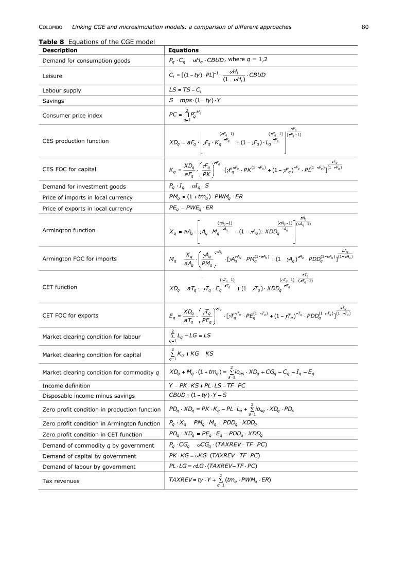
(2002). The CGE model for our economy (all equations are

presented in Table 8) is characterized by a representative household who maximizes a Cobb-Douglas utility function with three arguments: leisure and two consumption goods. These commodities are also used as inputs, together with capital and labour, in the production process, which is operated by two firms following a Leontief

technology in the aggregation of value added and

the intermediate composite good, a Constant

Elasticity of Substitution (CES) function for assembling capital and labour into value added,

and a Leontief function in the aggregation of intermediate goods. Both factors of production, capital and labour, are mobile among sectors. The capital endowment is exogenously fixed, while

labour supply is endogenously determined through household utility maximization (subject to fixed time endowment). The wage elasticity of labour supply is estimated from the household survey, in order to have consistency in labour supply behaviour between the two models. Investments are savings-driven, while government maximizes

a Cobb-Douglas utility function to buy consumption goods and uses labour and capital. The public sector also raises taxes on household income, places tariffs on imported goodsand pays transfers to households. For the foreign sector I have adopted the Armington assumption

(Armington, 1969) of constant elasticity of

substitution for the formation of the composite good (domestic production delivered to domestic market plus imports) which is sold on the domestic market. Domestic production is partially delivered to the domestic market and partially exported, according to a Constant Elasticity of

Transformation (CET) function. The small country hypothesis is assumed (the economy is price taker in the world market). In total the model comprises 49 variables and 41 equations, which, with the 8 exogenous variables (capital endowment, KS, time endowment, TS,

public transfers, TF, the four world prices PWEq and PWMq, and the numeraire, PC), fully determine the model and allow for satisfaction of Walras‟ law (we have a redundant equation).

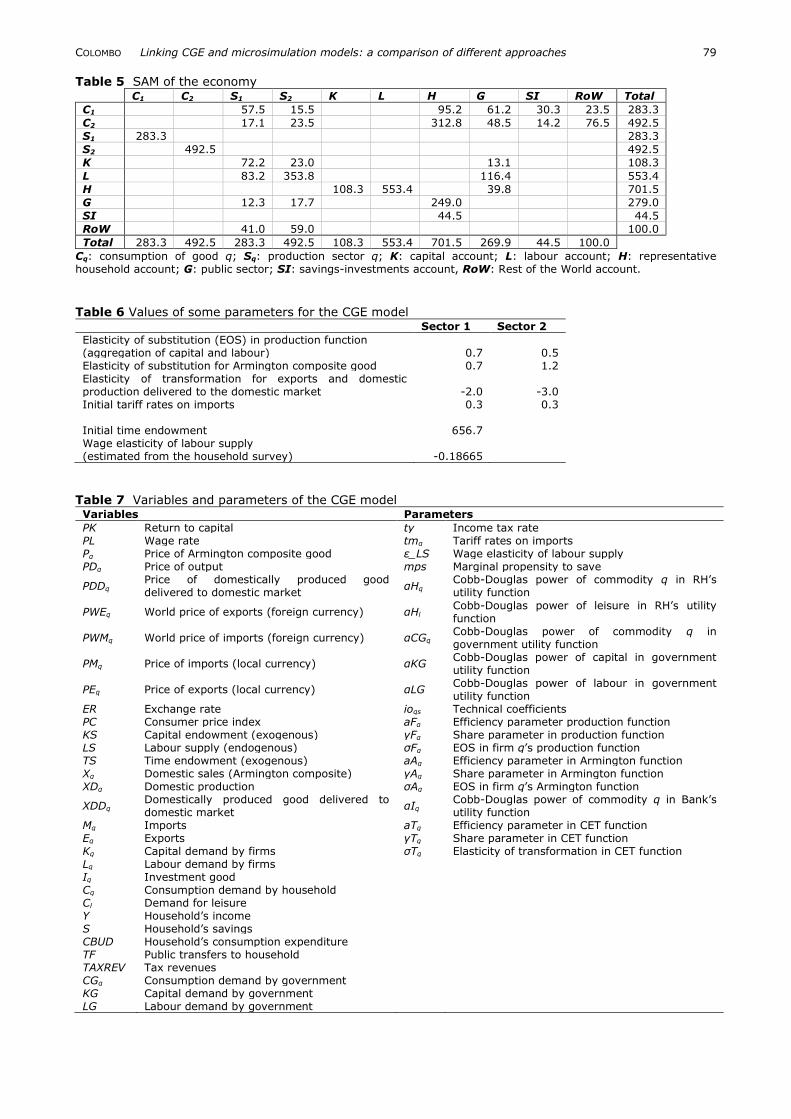
The calibration of the parameters of the CGE model is done on the basis of a Social Accounting

Matrix (SAM) for the economy. A SAM represents the flows of all economic transactions that take place within an economy. SAMs usually refer to a single year, thus providing a static picture of the economy. The columns of a SAM represent buyers (expenditures) and the rows represent sellers

(receipts). Columns and rows are added up to ensure accounting consistency, and each column is added up to equal each corresponding row. The SAM for the economy under study and the initial values of some other variables are consistent with the benchmark situation of the

micro-data (for instance, in the benchmark of the

two models I have the same average income tax rate, the same average marginal propensity to save, the same budget shares for consumption of the two goods, and so on). The SAM is reported in Table 5. Values of other initial parameters for the CGE module are shown in Table 6, while the

variables and equations used in the model can be found in Tables 7 and 8 below. The data in the SAM are in millions of the monetary unit used in the survey.


Table 5 SAM of the economy C1 C2 S1 S2 K L H G SI RoW Total

C1 57.5 15.5 95.2 61.2 30.3 23.5 283.3

C2 17.1 23.5 312.8 48.5 14.2 76.5 492.5

S1 283.3 283.3

S2 492.5 492.5

K 72.2 23.0 13.1 108.3

L 83.2 353.8 116.4 553.4

H 108.3 553.4 39.8 701.5

G 12.3 17.7 249.0 279.0

SI 44.5 44.5

RoW 41.0 59.0 100.0

Total 283.3 492.5 283.3 492.5 108.3 553.4 701.5 269.9 44.5 100.0

Cq: consumption of good q; Sq: production sector q; K: capital account; L: labour account; H: representative household account; G: public sector; SI: savings-investments account, RoW: Rest of the World account.

Table 6 Values of some parameters for the CGE model Sector 1 Sector 2

Elasticity of substitution (EOS) in production function (aggregation of capital and labour) 0.7 0.5 Elasticity of substitution for Armington composite good 0.7 1.2 Elasticity of transformation for exports and domestic production delivered to the domestic market -2.0 -3.0 Initial tariff rates on imports 0.3 0.3

Initial time endowment 656.7 Wage elasticity of labour supply (estimated from the household survey) -0.18665

Table 7 Variables and parameters of the CGE model Variables Parameters

PK Return to capital ty Income tax rate PL Wage rate tmq Tariff rates on imports Pq Price of Armington composite good ε_LS Wage elasticity of labour supply PDq Price of output mps Marginal propensity to save

PDDq Price of domestically produced good delivered to domestic market

αHq Cobb-Douglas power of commodity q in RH‟s utility function

PWEq World price of exports (foreign currency) αHl Cobb-Douglas power of leisure in RH‟s utility function

PWMq World price of imports (foreign currency) αCGq Cobb-Douglas power of commodity q in government utility function

PMq Price of imports (local currency) αKG Cobb-Douglas power of capital in government utility function

PEq Price of exports (local currency) αLG Cobb-Douglas power of labour in government utility function

ER Exchange rate ioqs Technical coefficients PC Consumer price index aFq Efficiency parameter production function KS Capital endowment (exogenous) γFq Share parameter in production function LS Labour supply (endogenous) σFq EOS in firm q‟s production function TS Time endowment (exogenous) aAq Efficiency parameter in Armington function Xq Domestic sales (Armington composite) γAq Share parameter in Armington function XDq Domestic production σAq EOS in firm q‟s Armington function

XDDq Domestically produced good delivered to domestic market

αIq Cobb-Douglas power of commodity q in Bank‟s utility function

Mq Imports aTq Efficiency parameter in CET function Eq Exports γTq Share parameter in CET function Kq Capital demand by firms σTq Elasticity of transformation in CET function Lq Labour demand by firms Iq Investment good Cq Consumption demand by household Cl Demand for leisure Y Household‟s income S Household‟s savings CBUD Household‟s consumption expenditure TF Public transfers to household TAXREV Tax revenues CGq Consumption demand by government KG Capital demand by government LG Labour demand by government


Table 8 Equations of the CGE model

Description Equations

Demand for consumption goods CBUDHCP qqq, where q = 1,2

Leisure CBUDH

HPLtyC

l

ll

)1(])1[( 1

Labour supply lCTSLS

Savings YtympsS )1(

Consumer price index 2

1q

Hq

qPPC

CES production function

)1()1()1(

)1(

q

q

q

q

q

q F

F

F

F

qqF

F

qqqq LFKFaFXD

CES FOC for capital )1()1()1(])1([ q

q

qqqq

q

F

F

FFq

FFq

F

q

q

qq PLFPKF

PK

F

aF

XDK

Demand for investment goods SIIP qqq

Price of imports in local currency ERPWMtmPM qqq )1(

Price of exports in local currency ERPWEPE qq

Armington function

)1()1()1(

)1(

q

q

q

q

q

q A

A

A

A

qqA

A

qqqq XDDAMAaAX

Armington FOC for imports )1()1()1(

])1([ q

q

qqqq

q

A

A

Aq

Aq

Aq

Aq

A

q

q

q

qq PDDAPMA

PM

A

aA

XM

CET function

)1()1()1(

)1(

q

q

q

q

q

q T

T

T

T

qqT

T

qqqq XDDTETaTXD

CET FOC for exports )1()1()1(

])1([ q

q

qqqq

q

T

T

Tq

Tq

Tq

Tq

T

q

q

q

qq PDDTPET

PE

T

aT

XDE

Market clearing condition for labour LSLGLq

q

2

1

Market clearing condition for capital KSKGKq

q

2

1

Market clearing condition for commodity q qqqqs

qqsqqq EICCGXDiotmMXD2

1

)1(

Income definition PCTFLSPLKSPKY

Disposable income minus savings SYtyCBUD )1(

Zero profit condition in production function 2

1ssqsqqqqq PDXDioLPLKPKXDPD

Zero profit condition in Armington function qqqqqq XDDPDDMPMXP

Zero profit condition in CET function qqqqqq XDDPDDEPEXDPD

Demand of commodity q by government )( PCTFTAXREVCGCGP qqq

Demand of capital by government )( PCTFTAXREVKGKGPK

Demand of labour by government )( PCTFTAXREVLGLGPL

Tax revenues 2

1

)(q

qq ERPWMtmYtyTAXREV


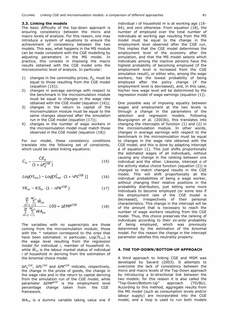
3.3. Linking the models

The basic difficulty of the top-down approach is ensuring consistency between the micro and

macro levels of analysis. For this reason, one may introduce a system of equations to ensure the achievement of consistency between the two models. This way, what happens in the MS module

can be made consistent with the CGE modelling by adjusting parameters in the MS model. In practice, this consists in imposing the macro results obtained with the CGE model onto the microeconomic level of analysis. In particular: 1) changes in the commodity prices, Pq, must be

equal to those resulting from the CGE model (equation (15));

2) changes in average earnings with respect to the benchmark in the microsimulation module must be equal to changes in the wage rate obtained with the CGE model (equation (16));

3) changes in the return to capital of the

microsimulation module must be equal to the same changes observed after the simulation run in the CGE model (equation (17));

4) changes in the number of wage workers in the microsimulation model must match those observed in the CGE model (equation (18))

For our model, these consistency conditions translate into the following set of constraints, which could be called linking equations:

)1( CGEq

qq

P

CEC (15)

)]1(ˆ[)( CGEmimi PLLYLogYLLog

(16)

)1( CGEmm PKKSYK (17)

CGE

m

NC

imi

m

NC

imi

EMP

WA

W

m

m

100

ˆ

24

1 1

24

1 1 (18)

The variables with no superscripts are those coming from the microsimulation module; those with the ^ notation correspond to the ones that

have been estimated: in particular, Log(ŶLmi) is the wage level resulting from the regression model for individual i, member of household m, while Ŵmi is the labour market status of individual

i of household m deriving from the estimation of the binomial choice model.

ΔPqCGE, ΔPLCGE and ΔPKCGE indicate, respectively,

the change in the prices of goods, the change in the wage rate and in the return to capital deriving from the simulation run of the CGE model, while parameter ΔEMPCGE

is the employment level percentage change taken from the CGE

framework. WAmi is a dummy variable taking value one if

individual i of household m is at working age (16-

64), and zero otherwise. From equation (18), the number of employed over the total number of

individuals at working age resulting from the MS model must be equal to the change in the employment level observed after the CGE run. This implies that the CGE model determines the

employment level of the economy after the simulation, and that the MS model selects which individuals among the inactive persons have the highest probability of becoming employed (if the employment level is increased from the CGE simulation result), or either who, among the wage workers, has the lowest probability of being

employed after the policy change (if the employment level is decreased), and, in this case, his/her new wage level will be determined by the regression model of wage earnings (equation (1)). One possible way of imposing equality between

wages and employment at the two levels is

through a change in the parameters of the selection and regression models. Following Bourguignon et al. (2003b), this translates into changing the intercepts of function (1) and (2) in the microsimulation module. In other words, changes in average earnings with respect to the

benchmark in the microsimulation must be equal to changes in the wage rate obtained with the CGE model, and this is done by adapting intercept a of equation (1). This just shifts proportionally the estimated wages of all individuals, without causing any change in the ranking between one individual and the other. Likewise, intercept α of

the activity status choice function (equation (2)) is changed to match changed results in the CGE model. This will shift proportionally all the individual probabilities of being a wage worker,

without changing their relative positions in the probability distribution, just letting some more individuals to become employed (or some less if

the employment rate of the CGE model is decreased), irrespectively of their personal characteristics. This change in the intercept will be of the amount that is necessary to reach the number of wage workers resulting from the CGE model. Thus, this choice preserves the ranking of

individuals according to their ex-ante probability of being employed, which was previously determined by the estimation of the binomial model. For this reason the change in the intercept parameter satisfies this neutrality property.

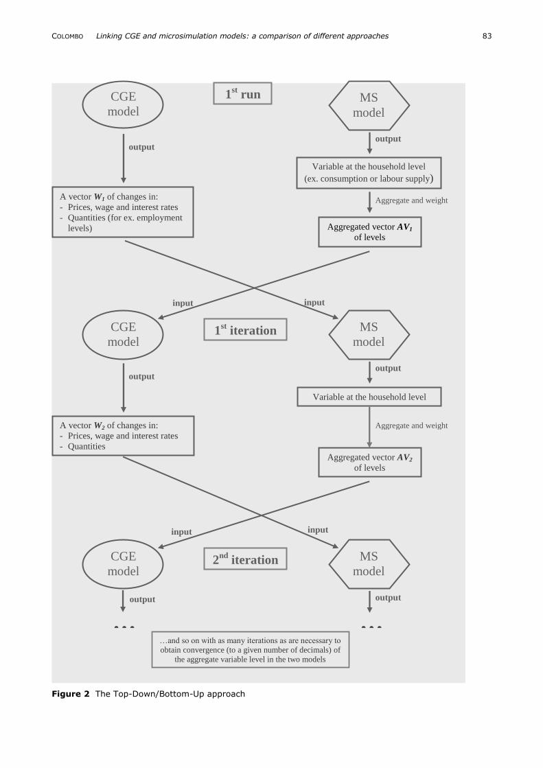
4. THE TOP-DOWN/BOTTOM-UP APPROACH

A third approach to linking CGE and MSM was developed by Savard (2003). It attempts to overcome the lack of consistency between the micro and macro levels of the Top-Down approach by introducing a bi-directional link between the

two models: for this reason it is also called the “Top-Down/Bottom-Up” approach (TD/BU). According to this method, aggregate results from the MS model (such as consumption levels and/or labour supply) are incorporated into the CGE model, and a loop is used to run both models


iteratively until the two produce convergent

results.

The value added of this approach is that it takes into account the feedback effects that come from the micro level of analysis, which are completely disregarded by the Top-Down model. The basic

assumption behind the TD/BU approach is that the microeconomic effects provided by the MS model run do not correspond to the aggregate behaviours of the representative households used in the CGE model, and that it is thus necessary to take these effects back into the CGE model to fully account for the effects of a simulated policy. A

stylized scheme of the way in which this approach works can be observed in Figure 2. The bilateral communication between the two levels of analysis is achieved through a set of vectors of changes, as in the Top-Down approach:

from the macro to the micro level of analysis

communication is guaranteed by the changes in the price, wage and return vector and in the employment levels, as before, while for communication from the micro to the macro level I consider in this paper two different strategies: in one, I use as input for the CGE model a vector of

changes in the aggregate consumption and in the labour supply levels from the MS model; in the other, only the change in the labour supply level which results from the MS model will be used as input for the CGE model. In either case the process is iterated as many times as is necessary to come to a convergent point, that is, when

convergence (at a certain number of decimals) is obtained in the aggregate variable levels of the two models.

The choice for consumption and labour supply as communicating variables is made following Savard (2003). However, as both consumption and labour

supply are not exogenous in the CGE model, some of the initial hypotheses of the model must be changed. First, I remove the equations determining consumption demand by the representative household (the first equation in Table 8), substituting them with the following

single equation:

2

1iii CPCBUD .

In the initial hypothesis (endogenous

consumption) I had two endogenous variables (Ci) and two equations. Now I have two exogenous

variables and one equation. As I need to insure the balancing of the household‟s budget constraint, a variable needs now to be endogenized in the following equation:

).(

)1()1(

TFLSPLKSPK

tympsCBUD

Following Savard, I choose to endogenize the marginal propensity to save, mps, which is now a

variable that changes in order to satisfy the budget constraint. In addition, I introduce an

exogenous level of labour supply into the CGE

model, and just leave out the equation that determines the demand for leisure (the second

equation in Table 8). This way, the third equation will now yield the demand for leisure as the time remaining after having supplied an exogenous level of labour. In the second variant of the TDBU

model, I introduce an exogenous level of labour supply into the CGE model, but omit the equation that determines the demand for leisure (the second equation in Table 8). 5. SIMULATION

Having outlined three alternative approaches to integrating CGE with microsimulation models, in this section I compare the results from each when used to simulate the same „policy‟. The simulation will be of an exogenous shock to the world price

level of the good exported by sector 2, which is

the labour intensive sector in our stylized economy. In this shock the world price of good 2 is reduced by 64% from its initial value. The simulation results for the most relevant macroeconomic variables are reported in

percentage changes in Tables 9 and 10. The macroeconomic results for the Top-Down model (shown in the second columns of the tables) represent the results that would emerge from a “stand-alone” CGE model, since they come from a simple run of the CGE model. These macroeconomic changes are then imposed onto

the microsimulation model, as explained in section 3.3, in order to obtain results at the micro level, which are shown in Tables 11 and 12.

In all tables, the two different strategies adopted for the TD/BU approach are also taken into account, allowing comparison of the results arising

from two different ways of taking into account the feedback effects from the micro level of analysis. This is done by introducing into the CGE model, as inputs derived from the microsimulation module, the consumption level and labour supply (C&LS), or the labour supply only (LS).

In general, for most of the macro variables, similar results are produced by all four simulations. The shock has negative effects on the economy. Indeed, as I can observe in Table 10, the fall in the price of the exported good for sector 2 causes a reduction of the production level for

this sector, which reduces its demand for both

factors of production. However, due to the depreciation of local currency, the reduction in the level of exports is lower than the 64% world price reduction. For the same reason, exports for the other production sector become more convenient, so that for this sector I observe an increase in the

level of the exported good, an increase in the production level, and in the demand for capital and labour. The depreciation of local currency also has a negative effect on the level of imports, which contributes to a decrease in the amount of goods sold on the domestic market.


Figure 2 The Top-Down/Bottom-Up approach

CGE

model

input input

output

A vector W1 of changes in:

- Prices, wage and interest rates

- Quantities (for ex. employment

levels)

Variable at the household level

(ex. consumption or labour supply)

Aggregated vector AV1

of levels

Aggregate and weight

output

CGE

model MS

model

1st run

output

input input

MS

model 1

st iteration

output

Aggregate and weight A vector W2 of changes in:

- Prices, wage and interest rates

- Quantities

Variable at the household level

Aggregated vector AV2

of levels

CGE

model

…and so on with as many iterations as are necessary to

obtain convergence (to a given number of decimals) of

the aggregate variable level in the two models

output

MS

model 2

nd iteration

…

output

…


Table 9 Simulation results: percentage changes (CGE model)

Integrated Approach

Top-Down Approach

TD/BU Approach (C&LS)

TD/BU Approach (LS)

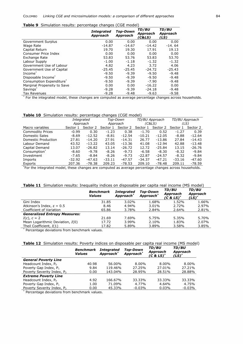
Government Surplus 0.00 0.00 0.00 0.00 Wage Rate -14.87 -14.67 -14.42 -14. 64 Capital Return 19.70 19.30 17.91 19.13 Consumer Price Index 0.00 0.00 0.00 0.00 Exchange Rate 53.83 53.76 53.83 53.70 Labour Supply -1.00 -1.18 -1.32 -1.32 Government Use of Labour 4.82 4.23 3.72 4.06 Government Use of Capital -25.45 -25.45 -24.72 -25.43 Income* -9.50 -9.39 -9.50 -9.48 Disposable Income* -9.50 -9.39 -9.50 -9.48 Consumption Expenditure* -9.50 -9.39 -7.90 -9.48 Marginal Propensity to Save 0.00 0.00 -16.22 0.00 Savings* -9.28 -9.39 -24.18 -9.48 Tax Revenues -9.28 -9.48 -9.63 -9.58 * For the integrated model, these changes are computed as average percentage changes across households.

Table 10 Simulation results: percentage changes (CGE model)

Integrated Approach

Top-Down Approach

TD/BU Approach (C&LS)

TD/BU Approach (LS)

Macro variables Sector 1 Sector 2 Sector 1 Sector 2 Sector 1 Sector 2 Sector 1 Sector 2

Commodity Prices -0.99 0.30 -1.23 0.38 -1.70 0.52 -1.27 0.39 Domestic Sales -8.69 -12.52 -8.81 -12.54 -10.21 -12.05 -8.88 -12.64 Domestic Production 27.81 -14.20 27.91 -14.31 26.77 -13.86 27.84 -14.43 Labour Demand 43.52 -13.22 43.05 -13.36 41.08 -12.94 42.88 -13.48 Capital Demand 13.07 -26.82 13.14 -26.72 12.72 -25.84 13.15 -26.76 Consumption* -8.60 -9.78 -8.26 -9.73 -6.58 -8.30 -8.32 -9.84 Investment -7.65 -8.84 -8.26 -9.73 -22.87 -24.57 -8.32 -9.84 Imports -32.92 -47.63 -33.11 -47.57 -34.37 -47.21 -33.16 -47.60 Exports 207.36 -78.38 209.23 -78.53 209.10 -78.48 209.11 -78.59 *For the integrated model, these changes are computed as average percentage changes across households.

Table 11 Simulation results: Inequality indices on disposable per capita real income (MS model)

Benchmark Values

Integrated Approach*

Top-Down Approach*

TD/BU Approach (C & LS)*

TD/BU Approach (LS)*

Gini Index 31.85 3.02% 1.68% 1.52% 1.66% Atkinson‟s Index, ε = 0.5 8.46 4.94% 3.01% 2.72% 2.97% Coefficient of Variation 65.86 3.78% 2.84% 2.64% 2.81%

Generalized Entropy Measures: I(c), c = 2 21.69 7.69% 5.75% 5.35% 5.70% Mean Logarithmic Deviation, I(0) 17.72 3.99% 2.10% 1.83% 2.07% Theil Coefficient, I(1) 17.82 5.89% 3.89% 3.58% 3.85% * Percentage deviations from benchmark values.

Table 12 Simulation results: Poverty indices on disposable per capita real income (MS model)

Benchmark Values

Integrated Approach*

Top-Down Approach*

TD/BU Approach (C & LS)*

TD/BU Approach (LS)*

General Poverty Line Headcount Index, P0 40.98 56.00% 8.00% 8.00% 8.00% Poverty Gap Index, P1 9.84 119.46% 27.25% 27.01% 27.21% Poverty Severity Index, P2 0.00 143.04% 28.95% 28.51% 28.88%

Extreme Poverty Line Headcount Index, P0 4.92 166.67% 33.33% 33.33% 33.33% Poverty Gap Index, P1 1.00 71.09% 4.77% 4.64% 4.75% Poverty Severity Index, P2 0.00 45.33% -0.03% 0.03% -0.03% * Percentage deviations from benchmark values.


The second sector is labour-intensive, as can be

observed in the SAM (Table 5). Therefore the level of labour demand as a whole falls, generating a

reduction in the wage rate, which causes a decrease in labour supply. The opposite is observed for capital, as the first sector is more capital-intensive. As a consequence of the change

in the price of the factors, government increases its demand for labour input and decreases the demand for capital, as the latter has become relatively more expensive. As the income of the representative household is based chiefly on the supply of labour, we observe

a reduction in nominal income and, as a consequence, of savings and consumption expenditure. The amount of consumption goods always decrease, but the percentage change varies according to the change in their relative price: the commodity produced by the second

sector has become relatively more expensive, due

to the negative shock that hit the sector. As investments are savings-driven, we also observe a reduction in the demand for investment goods (again, the investment good produced by the second sector is now relatively more

expensive, so I observe a higher reduction for the demand of this good). However, one particular result needs further explanation: savings and investments in the TD/BU-C&LS model decrease much more than in the other three models. The reason for this lies in

the fact that, in order to be able to introduce exogenous consumption levels into the CGE model, I had to endogenize one variable in the households‟ budget constraint to keep the

equilibrium in this constraint. Savard‟s choice is for the marginal propensity to save, and I have followed his approach. But the consequence of this

will be a change in household behaviour with respect to the initial assumptions made for the benchmark. Indeed, as Table 9 shows, the marginal propensity to save of the household decreased markedly; hence the greater decline in households‟ savings. As in our model investments

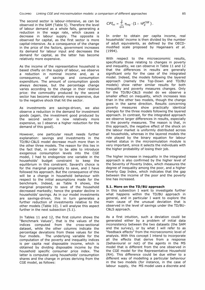
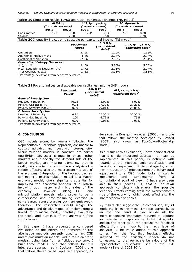
are savings-driven, this in turn generates a further reduction of investments relative to the other models (Table 10). I will analyse this aspect further in the next subsection (5.1). In Tables 11 and 12, the first column shows the “Benchmark Values”, that is the values of the

indices computed from the cross-sectional

dataset, while the other columns indicate the percentage deviations from these values for the four models. The underlying variable for the computation of the poverty and inequality indices is per capita real disposable income, which is obtained by dividing disposable income by the

household specific consumer price index. The latter is computed using households‟ consumption shares and the change in prices deriving from the CGE model, as follows:

2

1

)1(q

CGEqmqm PCPI .

In order to obtain per capita income, real households‟ income is then divided by the number of adult equivalents, as defined by the OECD-modified scale proposed by Hagenaars et al. (1994).

With respect to the microeconomic results, specifically those relating to changes in poverty and inequality, we can observe in Table 11 and 12 that the differences in results are generally significant only for the case of the integrated model. Indeed, the models following the layered

approach (namely the Top-Down and TD/BU models) show rather similar results for both inequality and poverty measures changes. Only for the TD/BU-C&LS model do we observe a

smaller effect on inequality, which increases less than in the other two models, though the change goes in the same direction. Results concerning

poverty measures show practically identical changes for the three models following the layered approach. In contrast, for the integrated approach we observe larger differences in results, especially in the poverty measures. The reason is that, in this approach, the negative effect of the shock on the labour market is uniformly distributed across

all households, whereas in the layered models the role played by the binary equation for labour market status in the microsimulation module is very important, since it selects the individuals with the higher probability of losing their job.

The higher increase in inequality in the integrated approach is also confirmed by the higher level of

the Severity of Poverty Index, which measures the degree of inequality among the poor, and a higher Poverty Gap Index, which indicates that the gap between the income of the poor and the poverty line has increased.

5.1. More on the TD/BU approach In this subsection I want to investigate further what happens within the TD/BU approach in general, and in particular I want to explore the main cause of the unusual deviation that is observed in the level of savings under the TD/BU-

C&LS approach. As a first intuition, such a deviation could be generated either by a problem of initial data inconsistency between the two datasets (the SAM

and the survey), or by what I will refer to as

“feedback effects” from the microeconomic level of analysis. With this concept I intend to incorporate all the effects that derive from a response (behavioural or not) of the agents in the MS model that is different from the one observed in the CGE model for the Representative Household (RH). This difference could be due either to a

different way of modelling a particular behaviour in the two models (for instance, in the case of labour supply, the MS model uses a discrete and


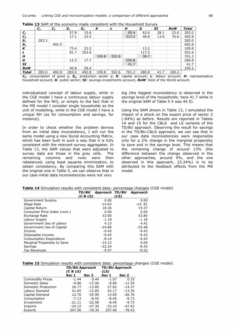
Table 13 SAM of the economy made consistent with the Household Survey C1 C2 S1 S2 K L H G SI RoW Total

C1 57.8 15.6 95.4 62.6 28.1 23.6 283.0

C2 17.1 23.5 313.2 48.8 13.6 76.6 492.8

S1 283.3 283.0

S2 492.5 492.8

K 73.4 23.2 13.2 109.8

L 81.7 353.8 117.5 552.6

H 109.8 552.6 38.7 701.2

G 12.3 17.7 250.8 280.8

SI 41.7 41.7

RoW 40.8 59.4 100.2

Total 283.0 492.8 283.0 492.8 109.8 552.6 701.2 280.8 41.7 100.2

Cq: consumption of good q; Sq: production sector q; K: capital account; L: labour account; H: representative household account; G: public sector; SI: savings-investments account, RoW: Rest of the World account.

individualized concept of labour supply, while in the CGE model I have a continuous labour supply defined for the RH), or simply to the fact that in the MS model I consider single households as the unit of modelling, while in the CGE model I have a

unique RH (as for consumption and savings, for

instance). In order to check whether the problem derives from an initial data inconsistency, I will run the same model using a new Social Accounting Matrix, which has been built in such a way that it is fully consistent with the relevant survey aggregates. In

Table 13, the SAM values that were adjusted to survey data are those in the grey cells. The remaining columns and rows were then rebalanced, using least squares minimization, to obtain consistency. By comparing this SAM with the original one in Table 5, we can observe that in

our case initial data inconsistencies were not very

big (the biggest inconsistency is observed in the savings level of the households: here 41.7 while in the original SAM of Table 5 it was 44.5). Using the SAM shown in Table 13, I simulated the

impact of a shock on the export price of sector 2

(-64%) as before. Results are reported in Tables 14 and 15 for the C&LS and LS variants of the TD/BU approach. Observing the result for savings in the TD/BU-C&LS approach, we can see that in our case data inconsistencies were responsible only for a 2% change in the marginal propensity to save and in the savings level. This means that

the remaining change of around 13% (the difference between the change observed in the other approaches, around 9%, and the one observed in this approach, 22.24%) is to be attributed to the feedback effects from the MS model.

Table 14 Simulation results with consistent data: percentage changes (CGE model)

TD/BU Approach (C & LS)

TD/BU Approach (LS)

Government Surplus 0.00 0.00 Wage Rate -14.63 -14. 81 Capital Return 18.36 19.37 Consumer Price Index (num.) 0.00 0.00 Exchange Rate 53.90 53.80 Labour Supply -1.18 -1.18 Government Use of Labour 4.13 4.42 Government Use of Capital -24.89 -25.48 Income -9.45 -9.43 Disposable Income -9.45 -9.43 Consumption Expenditure -8.14 -9.43 Marginal Propensity to Save -14.13 0.00 Savings -22.24 -9.43 Tax Revenues -9.57 -9.52

Table 15 Simulation results with consistent data: percentage changes (CGE model)

TD/BU Approach (C & LS)

TD/BU Approach (LS)

Sec 1 Sec 2 Sec 1 Sec 2

Commodity Prices -1.44 0.44 -1.07 0.33 Domestic Sales -9.86 -12.06 -8.89 -12.55 Domestic Production 26.77 -13.80 27.65 -14.27 Labour Demand 41.65 -12.85 43.17 -13.30 Capital Demand 12.70 -25.99 13.05 -26.76 Consumption -7.13 -8.45 -8.45 -9.73 Investment -21.11 -22.58 -8.45 -9.73 Imports -34.12 -47.30 -33.10 -47.63 Exports 207.50 -78.34 207.46 -78.43


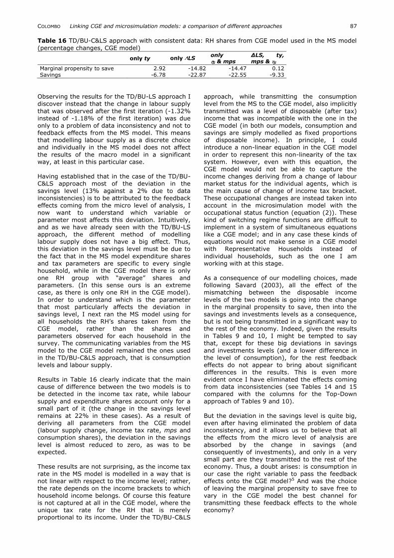
Table 16 TD/BU-C&LS approach with consistent data: RH shares from CGE model used in the MS model

(percentage changes, CGE model)

only ty only LS

only

i & mps ΔLS, ty, mps & i

Marginal propensity to save 2.92 -14.82 -14.47 0.12 Savings -6.78 -22.87 -22.55 -9.33

Observing the results for the TD/BU-LS approach I discover instead that the change in labour supply

that was observed after the first iteration (-1.32% instead of -1.18% of the first iteration) was due only to a problem of data inconsistency and not to feedback effects from the MS model. This means that modelling labour supply as a discrete choice and individually in the MS model does not affect

the results of the macro model in a significant way, at least in this particular case. Having established that in the case of the TD/BU-C&LS approach most of the deviation in the

savings level (13% against a 2% due to data inconsistencies) is to be attributed to the feedback

effects coming from the micro level of analysis, I now want to understand which variable or parameter most affects this deviation. Intuitively, and as we have already seen with the TD/BU-LS approach, the different method of modelling labour supply does not have a big effect. Thus, this deviation in the savings level must be due to

the fact that in the MS model expenditure shares and tax parameters are specific to every single household, while in the CGE model there is only one RH group with “average” shares and parameters. (In this sense ours is an extreme case, as there is only one RH in the CGE model).

In order to understand which is the parameter that most particularly affects the deviation in

savings level, I next ran the MS model using for all households the RH‟s shares taken from the CGE model, rather than the shares and parameters observed for each household in the survey. The communicating variables from the MS

model to the CGE model remained the ones used in the TD/BU-C&LS approach, that is consumption levels and labour supply. Results in Table 16 clearly indicate that the main cause of difference between the two models is to be detected in the income tax rate, while labour

supply and expenditure shares account only for a small part of it (the change in the savings level remains at 22% in these cases). As a result of deriving all parameters from the CGE model (labour supply change, income tax rate, mps and

consumption shares), the deviation in the savings

level is almost reduced to zero, as was to be expected. These results are not surprising, as the income tax rate in the MS model is modelled in a way that is not linear with respect to the income level; rather, the rate depends on the income brackets to which

household income belongs. Of course this feature is not captured at all in the CGE model, where the unique tax rate for the RH that is merely proportional to its income. Under the TD/BU-C&LS

approach, while transmitting the consumption level from the MS to the CGE model, also implicitly

transmitted was a level of disposable (after tax) income that was incompatible with the one in the CGE model (in both our models, consumption and savings are simply modelled as fixed proportions of disposable income). In principle, I could introduce a non-linear equation in the CGE model

in order to represent this non-linearity of the tax system. However, even with this equation, the CGE model would not be able to capture the income changes deriving from a change of labour market status for the individual agents, which is

the main cause of change of income tax bracket. These occupational changes are instead taken into

account in the microsimulation model with the occupational status function (equation (2)). These kind of switching regime functions are difficult to implement in a system of simultaneous equations like a CGE model; and in any case these kinds of equations would not make sense in a CGE model with Representative Households instead of

individual households, such as the one I am working with at this stage. As a consequence of our modelling choices, made following Savard (2003), all the effect of the mismatching between the disposable income

levels of the two models is going into the change in the marginal propensity to save, then into the

savings and investments levels as a consequence, but is not being transmitted in a significant way to the rest of the economy. Indeed, given the results in Tables 9 and 10, I might be tempted to say that, except for these big deviations in savings

and investments levels (and a lower difference in the level of consumption), for the rest feedback effects do not appear to bring about significant differences in the results. This is even more evident once I have eliminated the effects coming from data inconsistencies (see Tables 14 and 15 compared with the columns for the Top-Down

approach of Tables 9 and 10). But the deviation in the savings level is quite big, even after having eliminated the problem of data inconsistency, and it allows us to believe that all

the effects from the micro level of analysis are

absorbed by the change in savings (and consequently of investments), and only in a very small part are they transmitted to the rest of the economy. Thus, a doubt arises: is consumption in our case the right variable to pass the feedback effects onto the CGE model?5 And was the choice of leaving the marginal propensity to save free to

vary in the CGE model the best channel for transmitting these feedback effects to the whole economy?


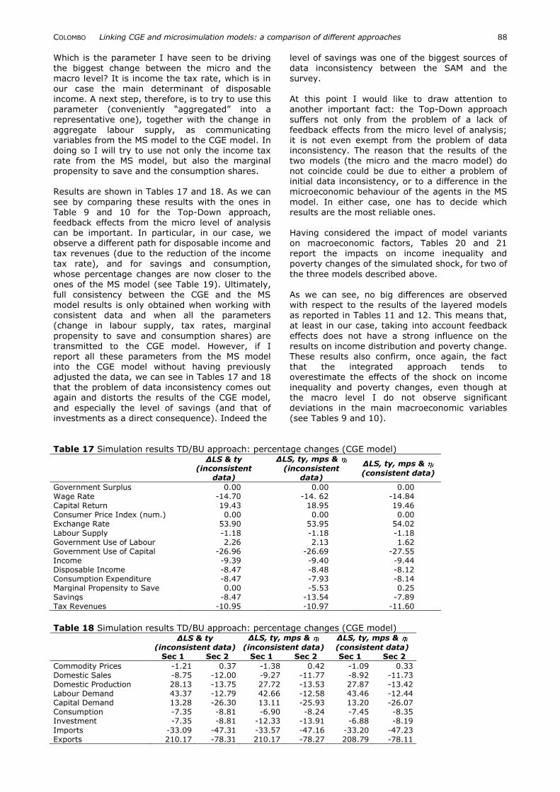
Which is the parameter I have seen to be driving

the biggest change between the micro and the macro level? It is income the tax rate, which is in

our case the main determinant of disposable income. A next step, therefore, is to try to use this parameter (conveniently “aggregated” into a representative one), together with the change in

aggregate labour supply, as communicating variables from the MS model to the CGE model. In doing so I will try to use not only the income tax rate from the MS model, but also the marginal propensity to save and the consumption shares. Results are shown in Tables 17 and 18. As we can

see by comparing these results with the ones in Table 9 and 10 for the Top-Down approach, feedback effects from the micro level of analysis can be important. In particular, in our case, we observe a different path for disposable income and tax revenues (due to the reduction of the income

tax rate), and for savings and consumption,

whose percentage changes are now closer to the ones of the MS model (see Table 19). Ultimately, full consistency between the CGE and the MS model results is only obtained when working with consistent data and when all the parameters (change in labour supply, tax rates, marginal

propensity to save and consumption shares) are transmitted to the CGE model. However, if I report all these parameters from the MS model into the CGE model without having previously adjusted the data, we can see in Tables 17 and 18 that the problem of data inconsistency comes out again and distorts the results of the CGE model,

and especially the level of savings (and that of investments as a direct consequence). Indeed the

level of savings was one of the biggest sources of

data inconsistency between the SAM and the survey.

At this point I would like to draw attention to another important fact: the Top-Down approach suffers not only from the problem of a lack of

feedback effects from the micro level of analysis; it is not even exempt from the problem of data inconsistency. The reason that the results of the two models (the micro and the macro model) do not coincide could be due to either a problem of initial data inconsistency, or to a difference in the microeconomic behaviour of the agents in the MS

model. In either case, one has to decide which results are the most reliable ones. Having considered the impact of model variants on macroeconomic factors, Tables 20 and 21 report the impacts on income inequality and

poverty changes of the simulated shock, for two of

the three models described above. As we can see, no big differences are observed with respect to the results of the layered models as reported in Tables 11 and 12. This means that, at least in our case, taking into account feedback

effects does not have a strong influence on the results on income distribution and poverty change. These results also confirm, once again, the fact that the integrated approach tends to overestimate the effects of the shock on income inequality and poverty changes, even though at the macro level I do not observe significant

deviations in the main macroeconomic variables (see Tables 9 and 10).

Table 17 Simulation results TD/BU approach: percentage changes (CGE model)

ΔLS & ty (inconsistent

data)

ΔLS, ty, mps & i

(inconsistent data)

ΔLS, ty, mps & i

(consistent data)

Government Surplus 0.00 0.00 0.00 Wage Rate -14.70 -14. 62 -14.84 Capital Return 19.43 18.95 19.46 Consumer Price Index (num.) 0.00 0.00 0.00 Exchange Rate 53.90 53.95 54.02

Labour Supply -1.18 -1.18 -1.18 Government Use of Labour 2.26 2.13 1.62 Government Use of Capital -26.96 -26.69 -27.55 Income -9.39 -9.40 -9.44 Disposable Income -8.47 -8.48 -8.12 Consumption Expenditure -8.47 -7.93 -8.14 Marginal Propensity to Save 0.00 -5.53 0.25 Savings -8.47 -13.54 -7.89 Tax Revenues -10.95 -10.97 -11.60

Table 18 Simulation results TD/BU approach: percentage changes (CGE model)

ΔLS & ty

(inconsistent data)

ΔLS, ty, mps & i

(inconsistent data)

ΔLS, ty, mps & i

(consistent data) Sec 1 Sec 2 Sec 1 Sec 2 Sec 1 Sec 2

Commodity Prices -1.21 0.37 -1.38 0.42 -1.09 0.33 Domestic Sales -8.75 -12.00 -9.27 -11.77 -8.92 -11.73 Domestic Production 28.13 -13.75 27.72 -13.53 27.87 -13.42 Labour Demand 43.37 -12.79 42.66 -12.58 43.46 -12.44 Capital Demand 13.28 -26.30 13.11 -25.93 13.20 -26.07 Consumption -7.35 -8.81 -6.90 -8.24 -7.45 -8.35 Investment -7.35 -8.81 -12.33 -13.91 -6.88 -8.19

Imports -33.09 -47.31 -33.57 -47.16 -33.20 -47.23 Exports 210.17 -78.31 210.17 -78.27 208.79 -78.11


Table 19 Simulation results TD/BU approach: percentage changes (MS model)

ΔLS & ty

(inconsistent data)

ΔLS, ty, mps & i

(consistent data) TD Approach

(inconsistent data)

Sec 1 Sec 2 Sec 1 Sec 2 Sec 1 Sec 2

Consumption -7.23 -8.28 -7.45 -8.35 -7.21 -8.28 Savings -7.78 -7.88 -7.78

Table 20 Inequality indices on disposable per capita real income (MS model)

Benchmark Values


data)*

ΔLS, ty, mps & i

(consistent data)*

Gini Index 31.85 1.70% 1.66% Atkinson‟s Index, ε = 0.5 8.46 3.04% 2.97%

Coefficient of Variation 65.86 2.86% 2.81%

Generalized Entropy Measures: I(c), c = 2 21.69 5.80% 5.70% Mean Logarithmic Deviation, I(0) 17.72 2.13% 2.07% Theil Coefficient, I(1) 17.82 3.93% 3.85% * Percentage deviations from benchmark values Table 21 Poverty indices on disposable per capita real income (MS model)

Benchmark Values


data)*

ΔLS, ty, mps & i

(consistent data)*

General Poverty Line Headcount Index, P0 40.98 8.00% 8.00% Poverty Gap Index, P1 9.84 27.30% 27.21% Poverty Severity Index, P2 0.00 29.01% 28.88%

Extreme Poverty Line Headcount Index, P0 4.92 33.33% 33.33% Poverty Gap Index, P1 1.00 4.79% 4.75% Poverty Severity Index, P2 0.00 -0.03% -0.03% * Percentage deviations from benchmark values

6. CONCLUSION CGE models alone, by normally following the Representative Household approach, are unable to capture individual and household heterogeneity.

Microsimulation models, in contrast, are partial

equilibrium analyses: change in prices, other markets and especially the demand side of the labour market are missing elements, that in reality are crucial for a complete analysis of a reform affecting also the macroeconomic side of the economy. Integration of the two approaches, connecting a microsimulation model to a macro-

economic model, offers significant potential for improving the economic analysis of a reform involving both macro and micro sides of the economy. However, linking CGE and microsimulation models might prove to be a cumbersome and time-consuming exercise in

some cases. Before starting such an endeavour, therefore, the researcher should weigh the advantages and disadvantages of implementing a

linked micro-macro model, carefully evaluating the scope and purposes of the analysis he/she wants to run.

In this paper I have presented a considered evaluation of the merits and demerits of the alternative methods currently used to link CGE and microsimulation models, with a focus on static models. Using data from a fictitious economy, I built three models: one that follows the full integrated approach, as in Cockburn (2001); one

that follows the so called Top-Down approach, as

developed in Bourguignon et al. (2003b), and one that follows the method developed by Savard (2003), also known as Top-Down/Bottom-Up model.

As a result of this evaluation, I have demonstrated

that a simple integrated approach, at least as implemented in this paper, is deficient with regards to the microeconomic specification and behavioural responses of individual agents, whilst the introduction of microeconometric behavioural equations into a CGE model looks difficult to implement and cumbersome from a

computational point of view. I have also been able to show (section 5.1) that a Top-Down approach completely disregards the possible feedback effects coming from the microeconomic side of the economy, which could affect also the macroeconomic variables.

My results also suggest the, in comparison, TD/BU modelling looks the most complete approach, as

on the one hand it can include all the microeconometric estimates required to account for behavioural responses by individual agents, and on the other take into account the feedback

effects from the micro to the macro level of analysis: “…The value added of this approach comes from the fact that feedback effects, provided by the household model, do not correspond to the aggregate behaviours of the representative households used in the CGE model» (Savard, 2003:20)”.


However, as my comparative evaluation has

shown, two main problems arise when using the TD/BU approach. First of all, the way in which

feedback effects are reported to the CGE model can affect results in a fundamental way. The use of shares or parameters, instead of absolute levels6, when possible, seems to lead to more

consistent results, in particular because when transmitting absolute levels from the MS model one has to change the initial hypothesis of the CGE model (see section 4). Secondly, eventual data inconsistencies between the micro and the macro datasets can also affect results seriously. This can only be overcome by adjusting one or

other dataset, thus going back to the problem of data reconciliation encountered with the integrated model (see section 2). However, whereas with an integrated model this problem is inevitably encountered when building the model, in a TD/BU model it is possible to run the model

without previously adjusting the data. In this

latter case, however, one is left unable to distinguish which is the part of the resulting change that is due to feedback effects and which is the part due to data inconsistencies. Acknowledgements

I would like to thank Stefan Boeters for his comments and suggestions. Notes 1 For early applications of this type of models,

see Adelman and Robinson (1978) and Dervis

et al. (1982), who specified lognormal within-group distributions with exogenous variances. More recent examples of this kind of models can be found in Decaluwé et al. (1999a),

Colatei and Round (2000) and Agénor et al. (2001).

2 After Mookherjee and Shorrocks‟ (1982) study

of UK, there are now other examples of “within/between” decomposition analysis of changes in inequality that indicate that changes in overall inequality are usually due at least as much to changes in within-group inequality as to changes in the between-group

component. Among the applications to developing countries, see Ahuja et al. (1997), who applied this decomposition analysis to the case of Thailand, and Ferreira and Litchfield (2001) for Brazil.

3 There exist different principles on which SAM-balancing programs can be based, such as the

“Row and Sum” or RAS method (see

Bacharach, 1971), least squares minimization principles, known also as Stone-Byron methods (see Stone (1977) and Byron (1978)), or the more recent cross-entropy approach proposed by Robinson et al. (2001) and Robilliard and Robinson (2003).

4 The Extreme Value distribution (Type I) is also known as Gumbel (from the name of the statistician who first studied it) or double exponential distribution, and it is a special case of the Fisher-Tippett distribution. It can take two forms: one is based on the smallest

extreme and the other on the largest. I will

focus on the latter, which is the one of interest for us. The standard Gumbel distribution

function (maximum) has the following probability and cumulative density functions, respectively:

pdf: )exp()( xexxf

CDF: )exp()( xexF . 5 Remember that in our case consumption is not

modelled in a significantly different way in the two models. However, there could be other cases where the level of consumption can be an important carrier of feedback effects from the micro level of analysis.

6 c.f. Savard (2003), in which consumption

levels are used. REFERENCES

Adelman I and Robinson S (1978) Income Distribution Policy in Developing Countries: A Case Study of Korea, Oxford: Oxford University

Press. Agénor P R, Izquierdo A and Fofack H (2001)

IMMPA: A Quantitative Macroeconomic Framework for the Analysis of Poverty Reduction Strategies, Washington: The World Bank.

Ahuja V, Bidani B, Ferreira F and Walton M (1997) Everyone’s miracle? Revisiting poverty and inequality in East Asia. Directions in Development, Washington: The World Bank.

Armington P S (1969) 'A Theory of Demand for Products Distinguished by Place of Production', IMF Staff Paper 16, 159-176.

Atkinson A B (1970) 'On the measurement of inequality', Journal of Economic Theory, 2,

244-263. Bacharach M (1971) Bi-proportional Matrices and

Input-Output Change, Cambridge: Cambridge University Press.

Boccanfuso D, Cissé F, Diagne A and Savard L

(2003) 'Un modèle CGE-Multi-Ménages Intégrés Appliqué à l‟économie Sénégalaise', miméo, CREA, Dakar, Codesria.

Bourguignon F, Robilliard A S and Robinson S (2003b) 'Representative versus real households in the macro-economic modelling of

inequality', DT/2003/10, DIAL/Unité de recherche CIPRE.

Bussolo M and Lay J (2003) 'Globalisation and Poverty Changes: A Case Study on Colombia', Working Paper No. 226, OECD Development Centre, Paris.

Byron R P (1978) 'The Estimation of Large Social

Accounting Matrices', Journal of the Royal Statistical Society, Series A, 141 (3).

Cockburn J (2001) 'Trade Liberalization and Poverty in Nepal: A Computable General Equilibrium Micro-simulation Approach', Working Paper 01-18, CRÉFA, Université Laval.

Cogneau D (2001) 'Formation du revenue,

segmentation et discrimination sur le marché du travail d‟une ville en développement: Antananarivo fine de siècle', DIAL DT/2001-18.

Cogneau D and Robilliard A-S (2001) 'Growth,


distribution and poverty in Madagascar:

Learning from a Microsimulation Model in a General Equilibrium Framework', IFPRI TMD

Discussion Paper No. 61 and DIAL DT/2001-19. Cogneau D and Robilliard A-S (2004) 'Poverty

Alleviation Policies in Madagascar: A Micro-Macro Simulation Model', DT/2004/11,

DIAL/Unité de Recherche CIPRÉ. Cogneau D and Robilliard A-S (2006) 'Simulating

targeted policies with macro impacts: Poverty Alleviation Policies in Madagascar', IRD, DIAL, Paris.

Colatei D and Round J (2000) 'Poverty and Policy: Some Experiments with a SAM-Based CGE

Model for Ghana', mimeo, Warwick University. Cororaton C B and Cockburn J (2005) 'Trade

Reform and Poverty in the Philippines: a Computable General Equilibrium Microsimulation Analysis', CIRPÉE, Working Paper 05-13.

Creedy J and Kalb G (2005) 'Discrete hours labour

supply modelling: specification, estimation and simulation', Journal of Economic Surveys, 19, 697-734.

Creedy J, Duncan A, Harris M and Scutella R (2002b) Microsimulation Modelling of Taxation and The Labour Market: The Melbourne

Institute Tax Transfer Simulator, Cheltenham: Edward Elgar.

Davies J B (2009) 'Combining microsimulation with CGE and macro modelling for distributional analysis in developing and transition countries', International Journal Of Microsimulation, 2(1), 49-65.

Decaluwé B, Patry A, Savard L and Thorbecke E (1999a) 'Poverty Analysis within a General Equilibrium Framework', Working Paper No. 99-09, African Economic Research Consortium.

Decaluwé B, Dumont J C and Savard L (1999b) 'Measuring Poverty and Inequality in a Computable General Equilibrium Framework',

Cahier de recherche du CRÉFA No. 99-20. Dervis K, de Melo J and Robinson S (1982)

General Equilibrium Models for Development Policy, New York: Cambridge University Press.

Duncan A and Weeks M (1998) 'Simulating transitions using discrete choice models',

Papers and Proceedings of the American Statistical Association, 106, 151-156.

Ferreira F H G and Litchfield J A (2001) 'Education or Inflation? The Micro and Macroeconomics of the Brazilian Income Distribution During 1981-1995', Cuadernos de Economia, 38, 209-238.

Hagenaars A, de Vos K and Zaidi M A (1994),

Poverty Statistics in the Late 1980s: Research Based on Micro-data, Luxembourg: Office for

Official Publications of the European Communities.

Heckman J J (1976) 'The common structure of statistical models of truncation, sample

selection and limited dependent variables and a simple estimator for such models', Annals of Economic and Social Measurement, 5(4), 475-492.

Heckman J J (1979) 'Sample Selection Bias as a Specification Error', Econometrica, 47(1), 153-162.

Hérault N (2005) 'A Micro-Macro Model for South Africa: Building and Linking a Microsimulation Model to a CGE Model', Melbourne Institute Working Paper Series, WP No. 16/05.

Löfgren H, Lee Harris R, Robinson S (2002) A standard Computable General Equilibrium

(CGE) model in GAMS, Microcomputers in

Policy Research, Vol. 5, Washington D.C.: International Food Policy Research Institute (IFPRI).

Lysy F J and Taylor L (1980) 'The General Equilibrium Income Distribution Model', in Taylor L, Bacha E, Cardoso E, Lysy F J (eds.),

Models of Growth and Distribution for Brazil, Oxford: Oxford University Press, Chapter 6.

Mookherjee D and Shorrocks A (1982) 'A Decomposition Analysis of the Trend in UK Income Inequality', Economic Journal, 92(368), 886-902.

Robilliard A-S and Robinson S (2003) 'Reconciling

Household Surveys and National Accounts Data Using a Cross Entropy Estimation Method', Review of Income and Wealth, 49(3), 395-406.

Robinson S, Cattaneo A and El Said M (2001)

'Updating and Estimating a Social Accounting Matrix Using Cross Entropy Methods', Economic Systems Research, 13 (1), 49-64.

Savard L (2003) 'Poverty and Income Distribution in A CGE-Household Micro-Simulation Model: Top-Down/Bottom-Up Approach', CIRPÉE Working Paper 03-43.

Stone R (1977) 'Forward' to G. Pyatt, A. Roe et al. (eds.), Social Accounting for Development

Planning with Special Reference to Sri Lanka, London: Cambridge University Press.

Date post:	06-Sep-2018
Category:	Documents
Upload:	doannga
View:	242 times
Download:	0 times

Linking CGE and Microsimulation Models: A Comparison of ... · Linking CGE and Microsimulation...

Documents