A new element of risk, liquidity risk, have flourished along this time taking importance and playing a key role in risk management tools. This has attracted the attention of the scientific community and economic and financial experts.
This thesis provides a theoretical introduction and a state of the art survey of the key elements needed to understand the complexity of the dealt issue. So it provides an study over liquidy risk and its application in market risk being included in market risk measures such as value at risk. Also an study over the behaviour of time series and it explores a relatively new alternative approach to model the liquidity risk using artificial neural networks, mainly approached in focused delay and recurrent neural networks due to their capability to work with time series .
In addition in this work have been designed and developed a methodology for the purpose of improving the way to treat time series and as resulting a simple graphical user interface with the intention of make easy the prediction.
This work has been developed on the framework Matlab Student Version version R2010a
including Neural Network Toolbox 6.0.4. over a laptop with Windows Vista 32 bits, CPU: Intel(R) Core(TM)2
Duo CPU 2.20GHz and RAM: 2038 MB.
4
ACKNOWLEDGEMENTS
I would like to thank my supervisors Dr. Salvador Torra Porras, Dr. Lluis Belanche and Dr. Maite López-Sánchez, for their support and dedication for reviewing my master thesis. Their unvaluable advices have meant a lot to me. Particularly to Dr.Salvador for introducing to me the world of risk analysis and to Dr. Lluis Belanche for showing to me excellent ideas.
In addition, I would like to thank to Guillerm Alfaro managing partner of www.solventis.es who provide me with dataset of equity market to be studied.
I would also like to thank my family, girlfriend and close friends for their support and
Related work ................................................................................................................................................ 13
Organization of this thesis ........................................................................................................................... 15
State of the Art ................................................................................................................................... 16
VaR: Value at Risk ........................................................................................................................................ 16
Time Series .................................................................................................................................................. 20
Basics of Time Series................................................................................................................................ 21
Exploring data .......................................................................................................................................... 34
Design of the GUI ......................................................................................................................................... 52
Code used .................................................................................................................................................... 54
List of Acronyms ...................................................................................................................................... 69
Usually, the discussion about liquidity risk flourishes afterward stock market crash but it’s a continuous problem of financial institution. Consequently asset liquidity risk is perhaps one of the prevalent treats facing today’s capital markets and has played a key role in major crises during the last two decades.
Taking into account that market liquidity is an asset's ability to be sold without causing a
significant movement in the price and with minimum loss of value1, sometimes, in rare liquidity conditions, there are asset positions can often not be traded close to fair prices and many risk management systems can’t predict it because they don’t include market liquidity risk metrics yet.
Furthermore in today’s days we are living a strangled period, the global financial crisis
which began in mid-2007, where many banks are struggled to maintain adequate liquidity. Unprecedented levels of liquidity support were required from central banks in order to sustain the financial system and even with such extensive support a number of banks failed, were forced into mergers or required resolution. Thus, due to the magnitude and nature of financial risk, the Basel Committee on Banking Supervision2 issued a package, called Principles for Sound Liquidity Risk Management and Supervision3 in September 2008 belonging to the Basel II Capital Accord, of proposals to liquidity regulations with the goal of promoting a more resilient banking sector. These sound principles provide key elements of a robust framework for liquidity risk management at banking organisation and among them there is the use of liquidity risk management tools such as comprehensive cash flow forecasting, limits and liquidity scenario stress testing. So, it opens the need of develop new tools that manage the liquidity risk. But attempting to summarize and approaching it at the current work, one of key advancement of the Basel II Capital Accord is the introduction of Value at Risk (VaR, risk measure of the risk of loss on a specific portfolio of financial assets4) as an internal risk measure to consolidate an institution’s market risk.
Looking into recent researches, I have found out that the conventional VaR approach to
computing market risk of a portfolio does not explicitly consider liquidity risk, but it only assess the worst change in mark-to-market portfolio value over a given time horizon. Therefore this technique does not differentiate between market and liquidity risk and is well-know that to ignore the liquidity risk can result in significant underestimation of the VaR estimate5.
The liquidity risk is assessed in concept of Bid-Ask spread or by adding an off-the-cuff
liquidity risk multiplier to the overall market risk exposure. Thus in order to improve the VaR models including well estimate liquidity risk I’ve focused my work on trying to forecast the bid-ask spread (the cost to unwind the trading positions) under the assumption that it works as a time series. 1 Website http://en.wikipedia.org/wiki/Market_liquidity
On the other hand I have considered use artificial neural networks (ANN) to modeling the
liquidity risk predicting the Bid-Ask spread so that the ANN are strongly used and many research papers justify that they are suitable in financial and economic time series ailments.
An Artificial Neural Network is an information processing paradigm which is inspired by the way biological nervous systems, such as the brain process information.
Figure 1: Biological Model
6
Figure 2: Mathematical Model
7
The first attempts are concerned to McCulloch and Pitts (1943) works. They developed
models of neural networks based on their understanding of neurology and they did simple models on logic functions, but were Rosenblatt (1958) who designed and developed the Perceptron. This system could learn to connect or associate a given input to a random output unit. Afterwards that increased up the number of research appearing enhancements models of networks and techniques like ADALINE (ADAptive LINear Element) which was developed by Widrow and Hoff (1960), Paul Werbos (1974) developed and used the back-propagation learning method, ART (Adaptive Resonance Theory) by Grossberg (1988), Self Organising Maps by Teuvo Kohonen (1989)...
As we can see the ANNs have an age of more 70 years old approximately and they have been rooted in many disciplines: neurosciences, mathematics, statistics, physics, computer science and engineering. Neural networks find applications in such diverse fields as modeling, time series analysis, pattern recognition, signal processing. This is consequently to the ANN capabilities provides like to learn and to generalize. Thus, the use of ANN offers useful properties: nonlinearity, Input-Output mapping, adaptivity and evidential response, very large scale integrated implementability (VLSI), uniformity of analysis and design, and neurobiological analogy. 6 Biological Model, website http://www.learnartificialneuralnetworks.com/images/bneuron.jpg
Furthermore according to the focus of this work the Artificial Neural Networks offer qualitative methods for business and economic systems that traditional quantitative tools in statistics and econometrics cannot quantify due to the complexity in translating the systems into precise mathematical functions8. Below I show the financial analysis task of which prototype neural network-based decision aids have been built9:
Credit authorization screening
Mortgage risk assessment
Project management and bidding strategy
Financial and economic forecasting
Risk rating of exchange-traded, fixed income investments
Detection of regularities in security price movements
Prediction of default and bankruptcy
Although the conventional models are certainly suitable to some tasks involving financial forecasting which works in well-identified models, the ANNs are best applied to problem environments that are highly unstructured. As I said above the ANN are useful in time series forecasting, thus considering that the current trouble is approached to time series models, it reinforces my proposal of solving it using artificial neural networks.
In first place, I’m going to define a little bit the term time series as a collection of observations made sequentially through time10 or as the evolution of a variable, phenomenon, over time and they can be economic, physical or social. An example is plotted below.
Figure 3: An example of time series: The GDP/PIB of Spain during 1980 until 2012
11
The scope of its studies is the knowledge of its pattern’s behaviour such that it let us make accurate predictions. Thus we could say that the main objectives of time-series analysis are to get a description of data usually using summary statistics and graphical models, to model it finding a suitable model which describes the data generating process (regards to ANNs techniques it is a big 8 According to Zahedi (1993)
9 Corresponding to Medsker (1996) list
10 Time Series Forecasting. Chris Chatfield (2001). pp. 1
11 The figure ilustrate the evolutio of the Spain GDP during the period of 1980-2010 more the prediction to 2012. The
data has been found in econstat.com. (last visit on 3 October 2010).
10
disadvantage because they are considerate like black-boxes), do forecasting to estimate the future values of the series and take control which means to take actions of control from good forecasts. Of course, though the future value of a time series cannot be predicted with absolute accuracy, the result cannot be fully random such that the study takes profit.
Thereby must have some regularity in its pattern’s behaviour which can be represented in
models. If in the case that we could predict without any error we’d are talking of deterministic phenomenon but normally the time series have associated random events which are named stochastic phenomenon.
Nowadays there are huge amounts of literatures references to time series analysis and
many researchers have come up with useful techniques based on classical model like ARIMA (autoregressive integrated moving average) or Box-Jenkins, ARMA (autoregressive moving average), GARCH (generalized autoregressive conditionally heteroscedastic model)... to forecast them but, however also there are alternative literature like Weigned and Gershenfeld (1994)12, Stern(1996)13, Warner and Misra(1996)14 and Faraway and Chatfield (1998)15 whose publications introduces ANNs in time series analysis and proof that it provides new features which are well-fitted to no-lineal and unstructured models.
12
Time Series Prediction. Weigned and Gershenfeld (1994). 13
Neural Networks in applied statistics. Stern(1996). 14
Understanding neural networks as statistical tools. Warner and Misra (1996). 15
Time Series Forecasting with neural networks: A comparative study using the airline data. Faraway and Chatfield (1998).
11
Motivation As I commented in the introduction, the banking organizations, afford to new regulations
introduced by Basel II Capital Accord, have the need of using liquidity risk management tools in order to improve their analysis of the risk. So, one way is to add the liquidity risk into VaR measures so that they do not explicitly consider liquidity risk. Hence I have focused my work on attempting to forecast the Bid-Ask Spread which is considered a measure of liquidity risk.
In addition, I have used Artificial Neural Networks so that their use is strongly arising in
financial and economic fields (and other approaches which are not of interesting in this work) even though they have to fight with classical statistical and econometrics models yet. Therefore, the main motivation of this work is to get optimal configuration of neuronal networks in order to proof its useful and helpful properties as forecaster (time series analysis) and consolidate them like suitable technique to solve real financial problems and underline their adaptable capabilities. For that, I’ve chosen a real and new ailment being this works one the first in apply NN in the liquidity risk problem.
On the other hand, is well-known that to configure the neural networks in order to reach
an optimal model is bored, large and complex process. Hence I would like to attempt to introduce a simple methodology and a tool in order to satisfy the needs of time series modelling. Thus, in order to summarize and to put into context, the following figure illustrates where I come from and where I go.
From current economic environment (crisis) crop up the need of including a new element of risk such as liquidity risk into already value-at-risk measures in order to minimize portfolio’s risk. Therefore, it forces to study this new component, its behaviour and to develop new techniques which let us to model and to forecast it with the purpose of minimizing its impact. So, one technique which is proposed by the market is the artificial neural networks.
12
Objectives
The neural networks have successfully been applied in different financial and economic fields and one of these have been to predict the behaviour of time series such as G. Peter Zhang and Douglas M. Kline(2007)16
, or Chan Man-Chung, Wong Chi-Cheong, Lam Chi-Chung17 show. Thus, I propose to model liquidity risk using artificial neural networks such as focused delay and recurrent neural networks. Therefore the main goal will consist of predicting the variable Bid-Ask Spread at t+1 (prediction for tomorrow) of a set of assets (35 assets provided by www.solventis.es) of the Spanish equity market.
To reach it, the work has been split in two main parts: 1. From a raw dataset and a model provided by financial experts, to indentify what
elements, features are important/significant to predict the bid-ask spread and what new elements can be introduced to improve its prediction.
2. To get an optimal model for each asset through a methodology developed by myself with automatizes the large steps to do in modeling time series.
As I have just commented, it also aims to make a contribution regards to time series
modeling using neural networks. For that it will be developed a methodology able to adapat inputs in order to allow us to get the optimal model over any time series, of course mainly the bid-ask spread time series will be the object of this work. Therefore, it will be composed by different methods which will afford to reach relevant properties of time series such as trend and number of delays (autocorrealtion). Also, in order to improve the parameter’s configuration of a network, it will be implementend few already proposed and well-known methods such as:
golden section search in order to find optimal number of neuron for a single layer
and a pruning algorithm to find what features improve the model.
In addition one purpose of this work is accomplish providing with a graphical user interface which allows someone to get prediction for new time series of some asset treated in this work. It will show prediction for t+h steps ahead where h will be fill in by the user.
16
Quarterly time-series forecasting with neural networks. G. Peter Zhang and Douglas M. Kline(2007). Working paper. 17
Financial time series forecasting by neural network using conjugate gradient learning algorithm and multiple linear regression weight initialization. Chan Man-Chung, Wong Chi-Cheong, Lam Chi-Chung. Working paper.
13
Related work First of all I would like denote that this work have cropped up due to the need of the
current economic and financial environment. Therefore it is not strange that I have not explicitly found any works related to the modeling of liquidity risk with neural networks. Otherwise, I have found few works talking about the need of include of liquidity risk in market risk measures (Value at Risk) and in other way some paper which apply neural networks to predict stock returns, volatility, volume traded.. which are strongly linked to liquidity risk and as the time series are treated to be used in neural networks.
Regarding to works of liquidity Risk, I have focused my efforts particulary in two recently
jobs. The first has been was written by Cornelia Ernst, Sebasting Strange and Christoph Kaserer on February 3, 200918 which are assessed different liquidity risk measure. They implemented Bangia et al. (1999)19, Giot and Gramming (2005)20, Stange and Kaserer (2008) 21and Ernst et al. (2008)22 in a large sample of dily sotck data over 5.5 years and they used a standar Kupiec (1995)23-statisitic to determine if model provide precise risk forecasts on a statistically significant basis. The provided results show that available data is the main driver of the preciseness of risk forecast, so the models get accurate performance depending of the data.
Specially this work is interesting because it provides a valuable information of what,
economic elements are related to liquidity risk. For instances Berkowitz (2000)24 and Cosandey(2001)25 developed related directly the volume or transaction with the liquitidy risk, or otherwise Francois-Heude and van Wynendaele (2001)26 linked it with the order size by using limit order book data27 or also find models in base of bid-ask spread as proposed by Bangia et al. (1999)28 and Ernst et al (2008)29.
The other one has been developed by Al Janabi, Mazin A. M on May 20, 2009 and they
present a generalized theoretical modeling approach for trading and fund management portfolios in base of liquidity risk model. This reflect the importance of liquidity risk given the rising need for measuring, managing and controlling of financial risk, trading risk prediction under liquid and illiquid market condition and also as it can be included to value-at-risk measures. It provides a 18
Measuring Market Liquidity Risk –Which model works best? Cornelia Ernst, Sebasting Strange and Christoph Kaserer(2009). 19
Liquidity on the Outside. Risk. Bangia, A., F. X. Diebold, T. Suchermann and J.D Stroughair (1999), pp. 68 – 73. 20
How large is liquidity risk in an automated auction market? Empirical economics. Giot, P. and J Gramming (2005), pp. 867 – 887. 21
Why and how to integrate liquidity risk into VaR-framewok. Stange, S. and C. Kaserer (2008). 22
Accounting for non-normality in liquidity risk. Ernst, C., S. Stange and C. Kaserer (2008). 23
Techniques for verifying the accuracy of risk management models. Kupiec, P. (1995), pp. 73 – 84. 24
Incorporating liquidity risk into value-at-risk models. Berkowitz (2000). 25
Adjusting value at risk for market liquidity. Risk. Cosandey, D (2001), pp. 115 – 118. 26
Integrating liquidity risk in a parametric intraday VaR framework. Francois-Heude, A. and P. Van Wynendaele (2001) 27
They use the liquidity cost measure ‘weighted spread’, which calculates the liquidity costs compared with the fair price when liquidating a position quantity q against the limit order book. 28
Liquidity on the outside. Riks. Bangia, A., F. X. Diebold, T. Schuermann and J.D. Stroughair (1999) pp 68 - 73 . 29
Accounting for non-normality in liquidity risk. Ernst, C., S. Stange and C. Kaserer (2008).
14
methodology for evaluating trading risk whe the impact of illiquidity of specified financial products is significant. Regarding to papers/works about neural networks used as preditor I have found many related works but however I have focused in which are strongly related with liquidity risk depedence. For instance, Mary Malliaris, Linda Salchenberger (1993)30 show that the neural networks are more able than the classical techniques to forecast the S&P 100 using implied volatily. To choose the best set of features they is begin with a small number of variables and add new variables which improve network performance. Summarizing they included 1331 variables where the remarkable thing is that delays were used only for volatility and neither detrend nor deseasonality the target. Their results were encouraging so that as they defend she neural network model, on the other hand, employs both short-term historical data and contemporaneous variables to forecast future implied volatility. Paul R. Lajbcygier and Jerome t. Connor (1997)32 concluded that somewhere between the hybrid neural network and the bootstrap predictor is best for this option pricing problem. Bootstrap methods for bias reduction was shown to give good results at the edge of input space where good extrapolation is critical. On the other hand Cottrell, M. (1995)33 while developing their methodology in base of combining statistical techniques of linear and nonlinear time series with the connectionist approach in order to simplify the architechture they concluded it was absolutely clear that such a multilayer perceptron cannot model a time series containing a trend. An other interesting paper which have substantained as treat of laggs of time series has been proposed by Huang Wei (2004) who provides a new methodology to seek optimal lag periods, which are more predictive and less correlated. All of theses papers/works provide some relevants characteristics which have been consisdered along of this work.
30
Using neural networks to forecast the S &P 100 implied volatility. Mary Malliaris, Linda Salchenberger (1996). 31
Neurocomputing 10 (1996) . M. Malliaris, L. Salchenberger, pp 190. 32
Improved option pricing using artificial neural networks and bootstrap methods. Paul R. Lajbcygier, Jerome t. Connor (1997). 33
Cottrell, M., Girard, B., Girard,Y., Mangeas, M., Muller, C., 1995. Neural modeling for time series: a statistical stepwise method for weight elimination. IEEE Transactions on Neural Networks 6 (6), pp. 1355–1364.
15
Organization of this thesis In this section I pretend to define the different sections of this work and as they are
organized. First of all, it has the introduction where I explain and put to the reader into the context of the work and immediately come the motivation and objectives points so that it help to reach and to clear the main aims of this work.
Secondly, once detailed what about my pretensions I introduce to the reader the keys topics for reinforcing the understanding, so giving an overview of value at risk, liquidity risk, time series and artificial neural networks and as they are linked under the State of Art section. The Value at risk topic/subsection is introduced in an easy way and finalized with dump example in order to make simple the concept. I have not got into more detail because it is not the main of the work and is enough to know its principle concept and not extensions.
According with Liquidity risk subsection, is explained how it has got importance over time
and I introduce two models where the liquidity risk is defined like the bid-ask spread and combined with VaR models to provide a more accurate evaluation of risk. Afterwards are defined the Time series and Artificial neural networks subsections. Again, as the value to predict is a time series, the Time series subsection pretends to introduce to the reader with an overview as they are treated and what important elements are contained in. In the last, and closing the key points is treated the Artificial neural networks topic where I have to denote that in this section have been emphasized the networks used or with pretension to use in this work and others have been left in second side.
In Platform develop section I explain in detail all the process that I followed to achieve the results detailed at the end of this work. It is divided by a main Description subsection where inform about the original dataset and as it composed. Afterward the Pre-process subsection comes Exploring data subsection which attempt to analyse the raw dataset looking for missing and outlier values, standardizing data and treat the trend and seasonality of time series. Feature selection subsection treat to find a common pattern in order to reduce or add some attributes.
One time is reached the goal of this section getting an efficient dataset the section
proceed with the definition of the Modeling subsection, where the reader can find a global diagram of the methodology used in order to choose the optimal network and also the detail of its components. Afterward the results are studied in Evaluating section.
As this work does not only pretend to be an study of forecasting the liquidity risk but also make a real application, hence in Practical application section have been designed a prototype of a graphical user interface which try to be an easy interface and to remove all complexity so that anyone will be able use it. To finalize, this work ends with Conclusion & Future works section providing what about of the thesis and possible new lines of research over this theme.
16
State of the Art
VaR: Value at Risk The value-at-risk (VaR) measures did not enter to financial field until early 20th century,
starting with an informal capital test the New York Stock Exchange (NYSE). It developed a set of requirements that the firms ought to hold (5% of customer debits, 10% (min.) on proprietary holdings in government bonds, 30% on proprietary holdings in other liquid securities and 100% on proprietary holdings in all other securities) for setting capital requirements.
In 1975, the US Securities and Exchange Commission (SEC) established a Uniform Net Capital Rule (UNCR)34 for US broker-dealers trading non-exempt securities. Thus, financial assets were split into 12 categories such as government debt, corporate debt, convertible securities, and preferred stock and additional haircuts were applied like any concentred position in a single asset. Although crude, the SEC’s system of haircuts was a VaR measure. Later, additional regulatory VaR measures were implemented for banks or securities firms.
Also VaR measures were influenced by portfolio theory, Markowitz (1952) and others independently published VaR measures to support portfolio optimization. For instances Lietaer (1971) describes a practical VaR measure for foreign exchange risk. So, over time VaR measures were increased quickly.
In 1990 appeared a new term risk management as the use of derivatives to hedge or customize market-risk exposures. The new risk management tends to view derivatives as a problem as much as a solution. It focuses on reporting, oversight, and segregation of duties within organizations. In July 1993 was published a report, named Group of thirty 30 report, which describes then derivatives use by dealers and end-users. The heart of the study is a set of 20 recommendations, a formal model (appear the concept of Value at Risk) for the evaluation of the such market risks for portfolios and trading desks over short periods of several trading days, to help dealers and end-users manage their derivatives activities, but though the report was focused on derivatives, most of its recommendations are applicable to the risks associated with other traded instruments.
The concept of VaR was taken up by financial regulator in the 1996 Basel Accord supplement and subsequently was extended to measuring credit risks over much longer horizons. It has gone arising until to become a major player in the enterprise-wide risk management solutions appropriate to the world’s financial institutions at all levels. Business activities entail a variety of risks which are distinguished between different categories of risks: market risk, credit risk, liquidity risk... although they have a strong correlation.
34
Annual report of the SEC for the fiscal year ended June 30, 1975, pp 17.
17
As market risk is defined as exposure to the uncertain market value of a portfolio35, such as we know the market value today but were are uncertain as to its market value a time ahead from today. Daily profits and losses on the contract reflect market risk.
Credit risk is defined as an investor's risk of loss arising from a borrower who does not make payments as promised36.
Liquidity risk as the risk of being unable to transact a desired volume of contracts at the current market price37.
Value-at-Risk is a category of market risk measures which let assess the potential loss of a trading or investment portfolio over some period of time. So summarizing, the notion is that losses greater than the value-at-risk are suffered only with a specified small probability. In particular, associated with each VaR measure are a probability α, or a confidence level 1-α, and a holding period, or time horizon, h. The 1-α confidence value-at-risk is simply the loss that will be exceeded with a probability of only α percent over a holding period of length h, equivalently, the loss will be less than the VaR with probability 1-α. For instances, if h is one day, the confidence level is 95% so that α=0.05 or 5% and the value-at-risk is one million euro, then over a one day holding period the loss on the portfolio will exceed one million euro with a probability of only 5%.
Thus, value-at-risk is a particular way of summarizing and describing the magnitude of the
likely losses on a portfolio. This makes it useful for measuring and comparing the market risks of different portfolios, for comparing the risk of the same portfolio at different times... But VaR’s simple, summary nature is also its most important limitation. Clearly information is lost when an entire portfolio is boiled down to a single number, its value-at-risk. This limitation has led to the development of methodologies for decomposing value-at-risk to determine the contributions of the various asset classes, portfolios, and securities to the value-at-risk. In addition it helps to overcome the problems in measuring and communicating risk information. Hence, due to its usefulness and applicability, there are many variations of VaR measures. The standard value-at-risk measure would be: VaR= (payoff in portfolio value) – k·(volatility’s portfolio), where k is set depending of confidence level.
1-α=84% k=1 1-α=95% k=1.645 1-α=97.5% k=2
Figure 4: Normal distribution with VaR value in base of its return
An easy example would be: X€ has been invested in an asset whose expected return is 15%
with a volatility of 10%. VaR with confidence-level of 95%:
VaR = 15%-1.645·10 = -1.45.
Its interpretation is with a 95 % of confidence level the potential loss is 1.45%, in other words with a probability of 95%, the investor will not lose more than 1.45%. But if we would have an upper expected return like E=20%, the investor wouldn’t have negative return, so the VaR would be 0.
VaR = 20%-1.645·10 = +3.45 => VaR=0.
Liquidity risk
Indeed the traditional VaR models is based in that the portfolio is stationary over the liquidation horizon and that the market is enoughly liquid to the market price is attainable by transactions prices. This marking-to-market approach is adequate to quantify and control sirk for an ongoing trading portfolio but may be more questionable if VaR is supposed to represent the worst loss over the unwinding period.
As I’ve explained above, in the introduction, market liquidity refers to the ability to undertake financial securities transactions in such a way as to adjust trading portfolio and risk exposure profiles without significantly disturbing prevailing market condition and underlying prices. In other words, is the risk that the liquidation value of trading assets may differ significantly form their current mark-to-market values and hence it is a function of the size of the trading positions, i.e. adverse price impac risk, and the price impact of trades, i.e. transactions cost liquidity risk38. Where the firs component, price impact , arises when the trader will sell out immediately by giving discount that brings the price down (the trader sells immediately at an unusually low price or buys at high price in case he had short sold assets) or however when the trader is unable to quickly sell a security at a fair price due to few people trade the given security, the second component, transactions cost liquidity risk, will be influenced.
Thus, it depends on the existence of enough number of counterparties and their readiness
to trade. Therefore, it sort of risk is strongly correlated with market risk, commented in VaR:Value at Risk section, which is increased under critical economical conditions due to its major variation (may mesured like volatility). But also we have to realize that there are markets illiquidity by themselves like can be corporative bonds.
Thereby, an unprivileged liquidity conditions indicates a relatively small number and size of
daily transactions and gives an indication of the size of a portfolio trading position than the market 38
Asset Market Liquidity Risk Management: A Generalized Theretical Modeling Approach for Trading and Fund Management Portfolios. Al Janabi, Mazin A.M (2009). pp12.
19
can absorb a given level. To get efficient models of liquidity risk is convenient and useful in order to optimization’ portfolio. Nowadays there are many models of liquidity risk which can be divided in two broad categories: traceable and theoretical.
A large literature has developed theoretical modeling approaches, these include more
recently to Subramanian and Jarrow (2001)39, Almegren (2003)40, Dubil (2003)41 and Engle and Ferstenberg (2007)
42. These models generally use optimal trading strategies to minimize the
Value-at-Risk of a position including liquidity. However, empirical estimation techniques for the large range of parameters of these models still need to be developed43.
Regarding to empirically traceable works we find to Bangia et aL (1999)44, Cosandey
(2001)45, Stange and Kaserer and Ernst et aL (2008)46. All proposed models can be grouped by the kind of required data for their estimation: bid-ask-spread models, transaction or volume data models, and models requiring limit order book data.
As the main goal of this work is the forecast of the liquidity risk in base of the bid ask
spread, I’m going to explain some models focused in bid-ask spread in order to understand how ithe liquidity risk is combined with VaR, also defined as L-VaR measure (value at risk of asset i under illiquid market conditions). But previously I should define Bid and Ask: Bid price is the price that somebody will pay for a stock at a given moment, while Ask price is the price at which someone is willing to sell a stock. Hence, the impact will be higher as the spread is higher and viceversa. For instances, if a trader trade 125 time along a year and the mid bid-ask spread is 1/8 (normal conditions), hence his cost of trade will add up to 125·1/8 = 15,625 and supposing that he trades with a capital of 50 per year. It means that the cost of winding will be 15,625/50 = 31,250% over his capital each year. In other words, If the trader want to make a profit, he will make it only after overcoming this 31.25% handicap. So that bid-ask spread has to be considered as you are trading.
Bangia, Diebold, Schuermann and Stroughair (1999)47 developed a simple liquidity
adjustment of a VaR-measure based on bid-ask-spread.
L-Var = 1 – exp(z𝜕𝑟)+(µs+𝑧𝑠 𝜎𝑠)
where 𝜕𝑟 is the variance of the continuous mid-price return over the appropriate horizon and µ𝑠 and 𝜎𝑠 are the mean and variance of the bid-ask spread, z is the percentile of the normal 39
The liquidity Discount, Mathematical Finance. pp: 447-474. 40
Optimal execution with nonlinear impact functions and trading-enhanced risk. Applied Mathematical finance, pp 11. 41
How to include liquidity in a Market VaR Statistic. Journal of Applied Finance, pp 19-28. 42
Execution Risk: It’s the Sme as Investment Risk. Journal of Portfolio Management, pp 34-44. 43
Cornelia Ernest, Sebastian Stange, Christoph Kaserer. Measuring Market Liquidity Risk. Which model Works best?, pp 2. 44 Liquidity on the outside. Risk, pp 68-73. 45 Adjusting Value at Risk for Market Liquidity. Risk, pp,115-118. 46 Accounting for Non-normality in Liquidity Risk. CEFS working paper 2008 No 14. Available at http://ssrn.com/abstract=1316769 47
Measuring market liquidity Risk: Which model works best?. pp 3.
distribution for the given confidence and 𝑧𝑠 is the empirical percentile of the spread distribution in order to account for non-normality in spreads.
Another model is proposed by Ernst, Stange and Kaserer48 who suggest a different way to
account for future time variation of prices and spreads. As it is more complex model and it is not the aim of this work, I am not going in depth.
Time Series As I have commented above, the variation of a variable over time is called time series (a
collection of random variables indexed according to the order they are obtained in time49). If we know its past behaviour (historical data) we could predict its possible future behaviours. Time series forecasting is a form of extrapolation in that it involves fitting a model to a set of data and them using that model outside the range of data to which it has been fitted50 . But, it’s not obviously as easy as seems such that we have to consider different assumptions like the dangers of extrapolation.
Therefore, we consider a time series such as x1, x2, ..., xn and the forecast future value such as xn+h where h is called the forecasting horizon or lead time. For instance, if h=1, the forecast future value will be n+h=n+1 where n is the current instant. So it means we’re forecasting for tomorrow. In general, a collection of random variables {xt}, indexed by t is referred as a stochastic process. Thus, a time series is a realization or sample function from a certain stochastic process.
Notice that we are talking about forecasting, hence, we have to reference to forecasting methods which are broadly classified into three types:
Judgemental methods regards to subjective intuition.
Univariate methods regards to single series. The prediction is based on one time series.
Multivariate methods regards to a predictable time series dependency. There’re one or more time series variables called predictor or explanatory variables which give relevant information about the predictable variable.
Usually forecasting methods combine more than one, for instance, when univariate or
multivariate methods are adjusted subjectively to take account of external information. In many cases is normally really difficult to distinct both approach and their combination get models better. For example, in particular, many macroeconomics forecasts are obtained by making adjustments to model-based forecasts, but, however it’s not always clear how such adjustments are made. So the combination of judgemental and statistical approach can improve the accuracy. 48
Accounting for Non-normality in Liquidity Risk. Ernst, C., S. Stange and C. Kaserer (2008), working paper. 49
Time Series Analysis and its Applications. Robert H.Sumway & David S.Stoffer. pp. 9. 50
Time Series Forecasting. Chris Chatfield (2001). pp. 7.
21
Coming back to the danger of extrapolation issue, we have to realize that forecasts are generally conditional statements of the form such “if this behaviour continues in the future, then...” which means that additional information in the future can produce a range of different forecasts. Even though there’re lot of examples which provide forecasts of years, we never can neglect that all forecasts are led by presumptions and a sudden change in the data can produce unexpected future values, so they cannot be predicted exactly but they do contain structure which can be exploited to make better forecasts.
Basics of Time Series
A common assumption in many time series techniques is that the data are stationary. A stationary process has the property that the mean, variance and autocorrelation structure do not change over time. Stationarity can be defined in precise mathematical terms, but for our purpose we mean a flat looking series, without trend, constant variance over time, a constant autocorrelation structure over time and no periodic fluctuations. Usually, in the classical methods there are two methodologies to study the behaviour of time series: modeling by components or Box-Jenkins approaches.
Modeling by component consist in attempt to identify four components, they are time
functions, which are not necessary exists together:
(T)Trend, defined as the long-term change in the underlying mean level per unit time. Usually it is expressed as time function of polynomial or logarithmic type: T=α0+ α1t+α2t2+…
If the data contain a trend, we can fit some type of curve to the data and then
model the residuals from that fit. Since the purpose of the fit is to simply remove long term trend, a simple fit, such as a straight line, is typically used.
For non-constant variance, taking the logarithm or square root of the series may
stabilize the variance. For negative data, you can add a suitable constant to make all the data positive before applying the transformation. This constant can then be subtracted from the model to obtain predicted (i.e., the fitted) values and forecasts for future points.
(S)Seasonal variation is defined as the oscillation which are given or repeated in short time periods. They can be associated to dynamic factors like hotel occupancy, the sale of clothings…
It is an important problem for forecasters. There are numerous models and many
different ways to analyze and forecast seasonal time series: a easy ways would be to use for instances, the run sequence plot which is a recommended first step for analyzing any
22
time series. Also, although seasonality can sometimes be indicated with this plot, seasonality is shown more clearly by the seasonal subseries plot or the box plot. The seasonal subseries plot does an excellent job of showing both the seasonal differences (between group patterns) and also the within-group patterns. The box plot shows the seasonal difference (between group patterns) quite well, but it does not show within group patterns. However, for large data sets, the box plot is usually easier to read than the seasonal subseries plot. Both the seasonal subseries plot and the box plot assume that the seasonal periods are known. In most cases, the analyst will in fact know this. For example, for monthly data, the period is 12 since there are 12 months in a year. However, if the period is not known, the autocorrelation plot can help.
But all of this models are well-suitable for specifics times series such as many
literature apoint that, but unfortunately no single model or modeling approach is best for all seasonal time series under different conditions as suggested by a large number of theoretical and empirical studies.
(C)Cyclic variation is given in long time periods and normally does references to economic states. As a rule they tend to be more difficult to indentify so its period is longer becau may there are enough recollected data to identify it.
(R)Irregular fluctuation, residue, is the random component belonging to noise.
The follow figure illustres all of this components:
Figure 5: Performing the seasonal decomposition for monthly beer 51
Thus, to assess the different components are used some statistical techniques such as moving average which are the most popular of them. Consequently, once identified all 51
The components have been obtained with the command stl of cran-R using the datafile http://134.76.173.220/beer.zip
components and assuming that the irregular fluctuation is additive we have two possible models called additive and multiplicative:
Additive Model: Y= T + S + C + R
Multiplicative Model: Y=T x S x C + R
Summarizing this model we can consider if seasonal pattern is constat along time it will be an additive model, but if this going amplifying while time, it will be a multiplicative model. In addition this classification is quite restrictive so that we can find mixed models.
Regarding to Box-Jenkins approaches, is based on determining what is the probability model governing thephenomenon’ behavior along the time. In other words, assuming that not ever we will be able to indentify the different components of serie, it study the randomly component (residue).
The statistical methodology used on this study is divided in 3 steps: 1)model identification, 2)parameter estimation and 3) diagnosis model. To achieve it we have several models like moving average (MA), autoregressive(AR), integrated(I) and their combinations (ARMA y ARIMA)52.
So far we have seen how to deal univariate time series analysis which only takes in account on past values of the same variable but perhaps theses past values depend also of other variables. Nowadays we find many examples where often the value of one variable is not only related to its predecessors in time but, in addition, it depends on past values of other variables. For instance, dealing with economic variables, household consumption expenditure may depend on variables such as income, interest rates, and investment expenditures. So if all these variables are related to the consumption expenditures it makes sense to use their possible additional information content in forecasting consumption expenditures. A general form could be:
y1,t+h=f(y1,t,y2,t,...,yk,t,y1,t-1,y2,t-1,…,yk,t-1,y1,t-2,…) where t is discrete time and h is the forecasting horizon.
This gives rise to a new set of techniques named vector time series models where we find the previous model adapted to multivariate factors: vector AR models, vector MA models, vector ARMA models, etc…
But I just wanted to put into context the reader as is treated time series from the classic prism, hence I will not go into depth in this theme because neither is the purpose of this work. Before to finalize this section, I would like to do the definition of autocorrelation that I commented above as a technique to now the period of seasonality.
52
For detailed treatment of ARMA and ARIMA see Time Series Analysis and its applications. Robert H Shumway and David S. Stoffer(2001). pp 89.
24
The autocorrelation plots are a commonly-used tool for checking randomness in a data set. This randomness is ascertained by computing autocorrelations for data values at varying time lags. If random, such autocorrelations should be near zero for any and all time-lag separations. If non-random, then one or more of the autocorrelations will be significantly non-zero. In addition, autocorrelation plots are used in the model identification stage for Box-Jenkins autoregressive, moving average time series models53.
Artificial Neural Networks The class of adaptive systems known as Artificial Neural Networks (ANN) were motivated
by the amazing parallel processing capabilities of biological brains (especially the human brain). The main motivation, at least initially, was to re-create these abilities by constructing artificial models of the biological neuron. The actual artificial neurons --as used in the ANN paradigm-- have little in common with their biological counterpart. Rather, they are primarily used as computational devices, clearly intended to problem solving: optimization, approximation of functions, identification of systems, classification, time-series prediction, and others.
The power of biological neural structures stems from the enormous number of highly
interconnected simple units. The simplicity comes from the fact that, once the complex electro-chemical processes are abstracted, the resulting computation turns out to be conceptually very simple. Artificial neurons are modeled to take profit of this by proposing simple computing devices that resemble the abstracted original function. However, in the ANN paradigm only very few elements are connected in most practical situations (on the order of hundreds, to say the most) and their connectivity is low. Therefore, it seems reasonable, once the ``biological origin'' is so departed, to think in compensating these low numbers by increasing the power of single units, while retaining the conceptual simplicity of seeing a neuron (a computational unit) as a em pattern recognizer: a device that integrates its incoming sources with its own local information available and outputs a single value expressing how much do they match.
Another aspect of the artificial neural networks is that there are different architectures,
which consequently requires different types of algorithms, but despite to be an apparently complex system, a neural network is relatively simple. The architectures used in this work are feed-forward. A mathematical model which represents you can find in Fig.2 page 8. From the illustrated model the interval activity of the
neuron can be shown to be 𝑣𝑘 = 𝑤𝑘𝑗 𝑥𝑗𝑝𝑗=1 .
In addition, the activation function acts as a squashing function, such that the output of a neuron in a neural network is between certain values (usually 0 and 1, or -1 and 1). In general, there are three types of activation functions, denoted by Φ(·) .
53 Engineering statistics handbook: Introduction to time series analysis. Available at http://www.itl.nist.gov/div898/handbook/eda/section3/autocopl.htm
First, there is the Threshold Function which takes on a value of 0 if the summed input is less than a certain threshold value (v), and the value 1 if the summed input is greater than or equal to the threshold value.
Secondly, there is the Piecewise-Linear function. This function again can take on the values of 0 or 1, but can also take on values between that depending on the amplification factor in a certain region of linear operation.
Thirdly, there is the sigmoid function. This function can range between 0 and 1, but it is also sometimes useful to use the -1 to 1 range. An example of the sigmoid function is the hyperbolic tangent function.
Learning algorithm
The property that is of primary significance for a neural network is the ability of this
network to learn from its environment, and to improve its performance through learning. The improvement in performance takes place over time in accordance with some prescribed measure. A neural network learns about its environment through an interactive process of adjustments applied to its synaptic weights and bias levels. Ideally, the network becomes more knowledgeable about its environment after each iteration of the learning process. A prescribed set of well-defined rules for the solution of a learning problem is called a learning algorithm. As one would expect, there is no unique learning algorithm for the design of neural network. Rather, we have a “kit of tools” represented by a diverse variety of learning algorithms, each of which offers advantages of its own. Basically, learning algorithms differ from each other in the way in which the adjustment to a synaptic weight of a neuron is formulated. Another factor to be considered is the manner in which a neural network made up of a set of interconnected neurons, relates to its environment.
There’re two kinds of learning: supervised and unsupervised. The current work only is focused on supervised learning. Thus, the supervised learning basically can be considered as learning with a teacher. In conceptual terms, we may think of the teacher as having knowledge of the environment, with that knowledge being represented by a set of input-output examples. Supposing that the teacher and the neural network are both exposed to a training vector, the teacher is able to provide the neural network with a desired response for that training vector. Indeed, the desired response represents the optimum action to be performed by the neural network. The network parameters are adjusted under the combined influence of the training vector and the error signal, taking account that the error signal is defined as the difference between the desired response and the actual response of the network.
One of the most well-known learning rules are the delta rule and its extension: back propagation algorithm. The delta rule, also called the Least Mean Square (LMS), was developed by Widrow and Hoff, method is one of the most commonly used learning rules. For a given input vector, the output vector is compared to the correct answer (for linear activation functions).
On the other hand for using nonlinear activation functions (tnh, log, sinh) the delta rule
26
have to be generalized: equations 𝛿𝑜𝑝 = (𝑑𝑜
𝑝 – 𝑦𝑜𝑝)Fo’(𝑠𝑜
𝑝) and 𝛿ℎ𝑝 = F’(𝑠ℎ
𝑝) 𝛿𝑜𝑝𝑤ℎ𝑜
𝑁𝑜
𝑜=1
give a recursive procedure for computing the δ's for all units in the network, which are then used to compute the weight changes according to equation. This procedure constitutes the generalised delta rule for a feed-forward network of non-linear units. So, we know from the delta rule that, in
order to reduce an error, we have to adapt its incoming weights according to △ 𝑤ℎ𝑜 =
𝑑𝑜 – 𝑦𝑜 𝑦ℎ .
But it delta rule manly is used for perceptron networks or only is able for a network with one layer. For treating with more layers was developed an extension which is called, back-propagation algorithm. So, in order to adapt the weights from input to hidden units, we again want to apply the delta rule. In this case, however, we do not have a value for δ for the hidden units. This is solved by the chain rule which does the following: distribute the error of an output unit o to all the hidden units that is it connected to, weighted by this connection. Differently put, a hidden unit h receives a delta from each output unit o equal to the delta of that output unit weighted with (= multiplied by) the weight of the connection between those units.
The application of the generalized delta rule thus involves two phases: During the first
phase the input x is presented and propagated forward through the network to compute the output values yp o for each output unit. This output is compared with its desired value do, resulting in an error signal δp for each output unit. The second phase involves a backward pass through the network during which the error signal is passed to each unit in the network and appropriate weight changes are calculated.
But as I said before, nowadays there are many learning algorithms. So in this study I have chosen the Bayesian regulation back-propagation54 which is provided by Matlab framework. It is based on updating the weight and bias values according to Levenberg-Marquardt optimization and minimizing a combination of squared errors and weights, and then determines the correct combination so as to produce a network that generalizes well.
54
MacKay (Neural Computation, Vol. 4, No. 3, 1992, pp. 415 to 447) and Foresee and Hagan (Proceedings of the International Joint Conference on Neural Networks, June, 1997) .
27
Types of neural networks
A brief overview about sort of neural networks we find that there are different ones but we could make a broadly classification grouping them in 2 categories: statics and dynamics networks. Static (feed-forward) networks have no feedback elements and contain no delays; the output is calculated directly from the input through feed-forward connections. However in dynamic networks, the output depends not only on the current input to the network, but also on the current or previous inputs, outputs, or states of the network.
Add delay make flourish the apparition of the term of time in neural networks which is considered as an essential dimension of learning. It has been incorporated into the design of a neural network implicitly or explicitly. For instances, a straightforward method of implicit representation of time is to add a short-term memory structure in the input layer of a static neural network (e.g., multilayer perceptron). The resulting configuration is sometimes called a focused time-lagged feed-forward network (TLFN) or focused time delay network (FTDN). So we can obtain the short-term memory structure may be implemented as Tapped-Delay-Line (TDL), even though exists other ways like Gamma Memory55 but they are not described here because they are not the focuses of this study.
Hence, the TDL is the most commonly used form of short-term memory. It consists of p
unit delays with p + 1 terminals, as shown in Fig. 6, which may be viewed as a single input–multiple output network. The unit-delay is denoted by z-1. The memory depth of a TDL memory is fixed at p, and its memory resolution is fixed at unity, giving a depth resolution constant of p.
Figure 6: ordinary tapped delay line memory of order p 56
Thus, summarizing this work is approached to use dynamic networks especially in already defined focused time-delay neural network (FTDNN) which consists in a feed-forward network with a tapped delay line at the input. The follow figure illustrates the typical network used in examples (overall in Matlab). 55
For detailed treatment of gamma memory see: An Analysis of the Gamma Memory in Dynamic Neural Networks. Jose C. Principe and Jyh-Ming Kuo, and Same1 Celebi (1994). 56 Feedforward Neural Networks: An introduction. Simo Hayken. pp. 12.
28
Figure 7: two-layer FTDNN 57
On the other hand, other sort of neural network which is useful to model nonlinearity of time series is the recurrent networks. They are neural networks with one or more feedback loops. The feedback exist whenever the output of an element in the system influences in part the input applied to that particular element, thereby giving rise to one or more closed paths for the transmission of signals around the system. The next figure is an example of a recurrent network which consist of a single layer of neurons with each neuron fiding its ouput signal back to the inputs of the other neurons.
Figure 8: Single layer of neurons with each neuron fiding its ouput signal back to the inputs of the other neurons
Thus, unlike the feed-forward networks, recurrent networks offers at least one feedback loop. The presence of feedback loops has a profound impact on the learning capability of the network and on its performance. Moreover, the feedback loops involve the use of particular branches composed of unit-delay elements which result in a nonlinear dynamical behaviour, assuming that the neural network contains nonlinear units.
There are many sort of recurrent networks, but as this study is developed under Matlab framework, among the recurrent networks provided the most recommended to model time series is a nonlinear autoregressive with exogenous inputs (NARX) model, hence I’m going to explain more in detail it. A generic recurrent network that follows naturally from a multilayer perceptron would be:
57 Two layer FTDNN, website http://www.mathworks.com/help/toolbox/nnet/dynamic3.html#34428
Figure 9: input that is applied to a tapped-delay-line memory of q units.
The model has a single input that is applied to a tapped-delay-line memory of q units. It has
a single output that is fed back to the input via another tapped-delay-line memory also of q units. The contents of these two tapped-delay-line memories are used to feed the input layer of the multilayer perceptron. The present value of the model input is denoted by u(n), and the corresponding value of the model output is denoted by y(n+1). That is, the output is ahead of the input by one time unit. Thus, the signal vector applied to the input layer of the multilayer perceptron consists of a data window made up as follows:
Present and past values of the input, namely u(n), u(n-1),...,u(n-q+1), which represent exogenous inputs originating from outside the network.
Delayed values of the output, namely y(n),y(n-1),...,y(n-q+1), on which the model output y(n+1) is regressed.
Thus, this recurrent network is referred to as a nonlinear autoregressive with exogenous
inputs (NARX) model. In Matlab is represented like:
Notice this type of neural network works with two kinds of delays, the first coming from
input values and the second from the output value.
Cross-Validation
Cross-validation is a method for estimating generalization error based on "resampling". The
resulting estimates of generalization error are often used for choosing among various models, such as different network architectures. In k-fold cross-validation, you divide the data into k subsets of (approximately) equal size. You train the net k times, each time leaving out one of the subsets from training, but using only the omitted subset to compute whatever error criterion interests you. If k equals the sample size, this is called "leave-one-out" cross-validation. "Leave-v-out" is a more elaborate and expensive version of cross-validation that involves leaving out all possible subsets of v cases. In this study has been developed a cross validation algorithm due to the lack in Matlab framework.
Feature selection
When we make some work, we have to recollect information; take measures of different
attributes linked to this problem and usually this process spend a lot of time and money. Every time we ask ourselves which features we could omit finding out which attributes are irrelevant or redundant in order to reduce the cost. In the literature we can find several definitions about feature selection. Some of them are:
Choosing a subset of the original features which will often lead to better performance.
Attribute selection is a pre-process step needed in unsupervised knowledge discovery in
order to reduce the number of irrelevant attributes that obfuscate the data.
Also known as variable selection, feature reduction, attribute selection, variable subset
selection, or dimension reduction is the technique, commonly used in machine learning, of
selecting a subset of relevant features for building robust learning models.
Pre-processing the data to obtain a smaller set of representative features, retaining the optimal salient characteristics of the data, not only decreases the processing time but also leads to more compactness of the models learned and better generalization. Others reasons for applying dimension reduction are:
Improve learning efficiency
Reduce the cost of measurements
31
Enable better understanding of the underlying process
Eliminate noise
Improve the prediction performance
Visualization
32
Platform Development
Description The raw dataset is composed by 78048x9 which provides 35 assets and the values of each
asset go from 03/01/2000 until 30/06/2010.
Name ISIN 1 ABENGOA SA ES0105200416
2 ABERTIS INFRAESTRUCTURAS SA ES0111845014
3 EBRO FOODS SA ES0112501012
4 BANCO BILBAO VIZCAYA ARGENTA ES0113211835
5 BANCO ESP CREDITO (BANESTO) ES0113440038
6 BANKINTER SA ES0113679I37
7 BANCO POPULAR ESPANOL ES0113790531
8 BANCO DE SABADELL SA ES0113860A34
9 BANCO SANTANDER SA ES0113900J37
10 BOLSAS Y MERCADOS ESPANOLES ES0115056139
11 GAS NATURAL SDG SA ES0116870314
12 INDRA SISTEMAS SA ES0118594417
13 FERROVIAL SA ES0118900010
14 FOMENTO DE CONSTRUC Y CONTRA ES0122060314
15 MAPFRE SA ES0124244E34
16 ACCIONA SA ES0125220311
17 ENDESA SA ES0130670112
18 ENAGAS ES0130960018
19 ACERINOX SA ES0132105018
20 CRITERIA CAIXACORP SA ES0140609019
21 OBRASCON HUARTE LAIN S.A. ES0142090317
22 GAMESA CORP TECNOLOGICA SA ES0143416115
23 IBERDROLA SA ES0144580Y14
24 IBERIA LINEAS AER DE ESPANA ES0147200036
25 IBERDROLA RENOVABLES SA ES0147645016
26 INDITEX ES0148396015
27 GESTEVISION TELECINCO SA ES0152503035
28 ACS ACTIVIDADES CONS Y SERV ES0167050915
29 GRIFOLS SA ES0171996012
30 RED ELECTRICA CORPORACION SA ES0173093115
31 REPSOL YPF SA ES0173516115
32 TECNICAS REUNIDAS SA ES0178165017
33 TELEFONICA SA ES0178430E18
34 SACYR VALLEHERMOSO SA ES0182870214
35 ARCELORMITTAL LU0323134006
Table 1: 35 assets of dataset
33
TAG Description Type
ISIN Asset’ ID numeric
DATE The date of trading session numeric
P_CLOSE The value of price of an asset in a trading session numeric
BID Bid price is the price that somebody will pay for a stock at a given moment.
numeric
ASK Ask price is the price at which someone is willing to sell a stock.
numeric
VOLUME Number of shares traded for one asset during the trading session, excluding applications and blocks
numeric
TURN_OVER Number of total shares traded for one asset during the trading session.
numeric
NUM_OP Number of operations done in a trading session numeric
CAPITAL The capital accumulated for one asset in one trading session numeric
Table 2: Raw dataset
This serie of features have been provided by experts, but it is easy to see as they are correlated with liquidity risk. According to the page 18, Liquidity risk section, the liquidity risk can be estimated in base of bid-ask-spread, transaction or volume data models. Then we have linked the bid, ask and volume features, but obviously the close price implicitly also is corresponded so that it will be the fair market price. Regarding the rest, some authors incorporate variation focusing on the use of high frequency transaction level data of stocks (see turn_over and num_op) according to their average transaction prices and capitalization. Even though the model proposed by the experts is:
TAG Description Type
VOLUME Number of shares traded for one asset during the trading session, excluding applications and blocks
numeric
TURN_OVER Number of total shares traded for one asset during the trading session.
numeric
NUM_OP Number of operations done in a trading session numeric
CAPITAL The capital accumulated for one asset in one trading session numeric
VOLATILITY Standard deviation of the profitability since 90 days ago Numeric
SPREAD The difference between BID and ASK Numeric
Table 3: Liquidity risk model provided by economic and financial experts
Where volatility and spread will be handled in Feature selection subsection. The ISIN and date are only informative attributes which are not used to get the model.
34
Pre-process
In pre-process I’ve noticed different tests to do in order to discard or choose an optimal characteristic/specific dataset instead of other. For instances, we can apply different methodologies to treat missing values, to normalize them or in the other hand remove tendency following the behaviour of classical models.
Exploring data
But first of all, it would be necessary get target value which is the difference between Bid and Ask. Thus, firstly I split the subset by ISIN such that each one represents a time series. So I have 35 subsets following this form:
TAG Description Type
P_CLOSE The value of price of an asset in a trading session numeric
BID Bid price is the price that somebody will pay for a stock at a given moment.
numeric
ASK Ask price is the price at which someone is willing to sell a stock. numeric
VOLUME Number of shares traded for one asset during the trading session, excluding applications and blocks
numeric
TURN_OVER Number of total shares traded for one asset during the trading session.
numeric
NUM_OP Number of operations done in a trading session numeric
CAPITAL the capital accumulated for one asset in one trading session numeric
Table 4: Form of subsets
Before to get the spread, I checked the missing values for each subset so the next subsection treat it in deep. Missing values
The missing values must be treated so that keeping them can be an inconvenient to apply afterward a policy optimization like standardizes inputs. Some ways to do it are:
To remove the observation which contain it: as we are working with time series it is not good idea so that we lose information and give up the sequence of time series.
To replace missing values by the mean what is not enough efficient so that in large period can have big variance and we can introduce noise.
To replace missing values searching the k neighbours is the most sophisticated and efficient way to treat it so that we’re searching for the nearest values of them.
35
I summarize how many missing values are distributed along of the raw dataset.
TOTAL
Size:78048
Attribute Number of missing %
P_CLOSE 2 0.0026
BID 56 0.0718
ASK 50 0.0641
VOLUME 57 0.0730
TURN_OVER 11591 14.8511
CAPITAL 1868 2.3934
NUM_OP 41539 53.2224
Table 5: Total percentages by each explicatory feature
For each missing values detail subset you can see the appendix in Missing detail section.
In order to get the spread I have decided to replace the missing values over BID and ASK features applying the mean between the 2 nearest values in basis of Standardized Euclidean distance over the premise that they are time series with low variance in a short period. Afterwards I obtain the spreads.
From the totals, the reader can see what features have most number of missing, they are bolded. So it is alarming the number of missing values in the feature num_op which is greater than 50 % of the total, thus it means that ½ of assets don’t have this value. So although I replace it using whichever optimal technique to I would probably provide a big error. Thus I could reformulate the initial model deleting it but previously I’m interested in knowing its weight in the model .
I have found three subsets which have no missing values in num_op field: ES0147645016, ES0187165017 and LU0323134006. Therefore in order to test their importance I have got correlation coefficients and their p-values so that it let me to know how much they are linearly correlated to the target.
ISIN Corr. p-value
ES0147645016 0.1551 7,8025e-05
ES0187165017 0.0507 0,1049
LU0323134006 0.1610 3,2439e-07
Table 6: coef. Correlation and p-values obtained of Spread versus num_op features
As above results show, all of them are insignificant producing a correlation coefficients very lowers (justified by their p-values except for ES0187165017). Therefore, we could say that there is not lineal correlation between bid-ask spread and num_op. Furthermore, I’ve done another experiment to contrast the relevance of num_op.
For each of the 3 subsets described above, I’ve trained a feed-forward time delay network with and without the attribute num_op and fixing the parameters:
36
Type Train.
Alg.
# Neurons TDelay Stand. CV Error
FFTD Trainrb 30 2 Mean=0 Std=1
10 MSE NRMSE
Table 7: parameters of neural network
ISIN Num_op NRMSE
ES0147645016 With 1.4113
Without 1.3545
ES0187165017 With 6.7169
Without 6.2927
LU0323134006 With 1.8453
Without 1.8345
Table 8: results of with and without num_op attribute
Checking the results above, we can notice that in base of the error in all cases we obtain lower error without the feature num_op. So, further we can add that practically don’t exist lineal correlation, thus we can infer that num_op is irrelevant or does not provide useful information, hence I have chosen do the experiments without it.
In addition, we saw that capital and turn_over features have a large percentage overall in
some specifics subsets. Thus, I have taken subsets with the treated features completely full and following the methodology used in previous case, I have performanced the experiments to attempts to find out the lineal and non-lineal correlation between these features and the target.
ISIN Corr. p-value
ES0113900J37 -0.0565 0.0036
ES0115056139 0.0437 0.1657
ES0171996012 0.0481 0.1195
ES0173093115 -0.0458 0.0008
ES0187165017 -0.0460 0.1419
ES0178430E18 -0.0678 0.0005
Table 9: coef. correlation and p-values obtained of Spread versus capital features
ISIN Capital NRMSE
ES0113900J37 With 2.3222
Without 1.8837
ES0115056139 With 1.2489
Without 1.2542
ES0171996012 With 2.0212
Without 1.7427
ES0173093115 With 2.1305
Without 1.425
ES0187165017 With 1.6938
Without 1.1433
ES0178430E18 With 1.0711
Without 1.0697
Table 10: results of with and without capital attribute
If we check both cases, we find out that there are cases with particular behaviour. Focusing
in first set, where were analyzed 6 subsets with capital feature, we find that all of them have a low lineal correlation but only three of them (ES0113900J37, ES0173093115, ES0178430E18) the results are significative (p-value higher than 0.05). In other hand, looking for a non-lineal correlation, the same subsets were analyzed in base of the results from ANN. In that way, we find that 5 subsets
37
have not significance information to predict the spread: ES0113900J37, ES0171996012,
ES0173093115, ES0187165017, ES0178430E18. Otherwise the remainder subset, ES0115056139, shows a very little improvement 1.2489 versus 1.2542 which may be due to noise component. Thus, summarizing we may infer that the capital feature can be remove from the original dataset.
ISIN Corr. p-value
ES0113860A34 -0.0091 0.6606
ES0113211835 -0.0781 0.0001
ES0113679137 0.0560 0.0040
ES0124244E34 0.0431 0.0267
ES0113790531 -0.0092 0.6359
ES0115056139 0.0833 0.0082
ES0118594417 -0.0677 0.0005
ES0118900010 -0.0033 0.8991
ES0122060314 -0.0147 0.4507
ES0171996012 0.0374 0.2263
Table 11: coef. correlation and p-values obtained of Spread versus turn_over features
ISIN Turn_over NRMSE
ES0113860A34 With 1.0457
Without 1.0408
ES0113211835 With 1.2337
Without 1.2309
ES0113679137 With 4.8211
Without 2.2451
ES0124244E34 With 1.0742
Without 1.0755
ES0113790531 With 2.9945
Without 1.3809
ES0115056139 With 1.2181
Without 1.0879
ES0118594417 With 1.117
Without 1.1724
ES0118900010 With 1.0099
Without 1.0135
ES0122060314 With 1.0919
Without 1.1735
ES0171996012 With 1.2655
Without 1.1966
Table 12: results of with and without turn_over attribute
Regarding to the second set, it is composed by 10 assets which have been analyzed with and without turn_over feature. From the results, table 11 we find out that again all of them show a low correlation even though only five (ES0113211835, ES0113679137, ES0124244E34, ES0115056139, ES0118594417) are significant. According to table 12 we find that 7 of them (ES0113860A34, ES0113211835, ES0113679137, ES0124244E34, ES0113790531, ES0115056139, ES0171996012) achieve a lower error. In other words, the turn_over feature don’t provide useful inforfmation to the neural network . So due to almost of subsets have missing values and that the results show a better perfomance without the feature I have also decided to remove it from the original dataset. Summarizing, from of three features to be study I have removed so that they have a high number of missing values and keep them in input set didn’t enhance perfomance such as show a their really lower correlation with the feature to be predicted.
38
Outliers Outliers are data values that are dramatically different from patterns in the rest of the
data. They may be due to measurement error, or they may represent significant features in the data. Identifying outliers, and deciding what to do with them, depends on an understanding of the data and its source.
Thus, from the dataset without missing values are identified the possible outliers where an outlier is defined as a value that is more than three standard deviations away from the mean. In total terms, the proportion of outliers looks no relevant but it is important how they are distributed.
Tabla 10: Outliers of raw dataset showed in number of elements and %
In mode of guide, I have commented in deep the asset ES0113860A34.
P_CLOSE BID ASK VOLUME TURN_OVER CAPITAL NUM_OP
Outliers 0 0 0 25 27 0 49
% 0 0 0 0.0108 0.0116 0 0.0211
Table 11: Outliers of the subset ES0113860A34
Figure 11: P_CLOSE outliers
Figure 12: BID outliers
Figure 13: ASK outliers
Figure 14: VOLUME outliers
Figure 15: TURN_OVER outliers
Figure 16: CAPITAL outliers
2 3 4 5 6 7 8 9 100
100
200
300
400
500
600
Data
Mean
Stds
2 3 4 5 6 7 8 9 100
100
200
300
400
500
600
Data
Mean
Stds
2 3 4 5 6 7 8 9 100
100
200
300
400
500
600
Data
Mean
Stds
0 0.5 1 1.5 2 2.5 3 3.5 4 4.5
x 107
0
200
400
600
800
1000
1200
1400
1600
1800
2000
Data
Mean
Stds
0 1 2 3 4 5 6 7 8 9
x 108
0
500
1000
1500
2000
2500
Data
Mean
Stds
2000 4000 6000 8000 10000 12000 140000
50
100
150
200
250
300
350
400
450
500
Data
Mean
Stds
39
How is showed in above table and the followed figures, particularity in this case, the number of outliers in subset almost is not relevant being lower of 1% the amount of each one for each feature. So in this case, the outliers could be considerate like extreme value but not incorrect. In general cases the highest is over 2.0770% of deviation, equally it is a low percentage so the bias that can produce is minimum. If the reader want to check the rest of outliers, he can find in Appendix, Outliers Details section. Standardize data
Following the theory it usually advises standardize the values in order to optimize algorithms for weight determination in neural networks avoiding saturate them and as consequence they lose capacity to learn. So in order to define it we can say that normalizing, in the NN literature, mostly it refers to rescaling by the minimum and range of the vector, to make all the elements lie between 0 and 1.
In the literature we can find different cases, for example: If the input variables are combined via a distance function (such as Euclidean distance) in an RBF network, standardizing inputs can be crucial, but if the input variables are combined linearly, as in an MLP, then it is rarely strictly necessary to standardize the inputs, at least in theory. The reason is that any rescaling of an input vector can be effectively undone by changing the corresponding weights and biases, leaving you with the exact same outputs as you had before. However, there are a variety of practical reasons why standardizing the inputs can make training faster and reduce the chances of getting stuck in local optima. The main emphasis in the literature on initial values has been on the avoidance of saturation, hence the desire to use small random values. How small these random values should be depends on the scale of the inputs as well as the number of inputs and their correlations. Standardizing inputs removes the problem of scale dependence of the initial weights.
I show a little proof attempting to demonstrate it. Consider an MLP with two inputs (X and Y) and 100 hidden units and comparing the inputs over the interval [-10, 10] and the interval [-1, 1].
Figure 17: NUM_OP outliers
0 1000 2000 3000 4000 5000 6000 70000
200
400
600
800
1000
1200
Data
Mean
Stds
40
Figure 19: Hiperplanes over range [-1,1]
We can observe that in first figure where the range is over [-10, 10] the most of hyperplanes are concentrated in the centre missing the corners, so if the networks needs to learn such a hyperplane may take many random initializations before training finds a local optimum with such a hyperplane. On the other hand, if we rescale the range of input values, we find a totally different picture where we check that the hyperplane are more successfully distributed along the range easing the learning.
So normalization data is an important factor to consider, and in addition in the literature is found a close relation with transfer function in order to match the range of the outputs where logistic or hyperbolic tangent function has a typical range of [0,1] and [-1,1] respectively.
Thus, I’ve done a few proofs in order to evaluate which range is more efficient in the present case.I have taken the first results of num_op from outlier section (page 25) which are done using mean 0 and standard deviation 1 versus a range -1,+1.
Type Train.Alg. # Neurons TDelay CV Error
FFTD Trainrb 30 2 10 MSE NRMSE
Table 13:parameters of neural network
Stand. ISIN MSE NRMSE
m=0, std=1 ES0147645016 0.00029001 1.3545
m=0, std=1 ES0187165017 0.29644 6.2927
m=0, std=1 LU0323134006 0.059013 1.8345
-1 , +1 ES0147645016 0.00015031 1.1868
-1 , +1 ES0187165017 0.033037 1.1174
-1 , +1 LU0323134006 0.047977 1.2322
Table 14: results of whit and without num_op attribute
The above results show working with range -1, +1 the NN obtain better results than standardizing to mean=0 and deviation 1.
Figure 18: Hiperplanes over range [-10,10]
41
Trend
The trend effect play a relevant role at the moment of modeling a time series due to its presences can produce a bad learning of the neural network, thus it should be treated. Several researches denoting that for a forecasting problem which involves continuous target values, it is reasonable to use a linear activation function for output nodes. Even so, the ANNs with linear output have the limitation that they cannot model a time series containing a trend (Cottrell, M., Girard, B., Girard,Y., Mangeas, M., Muller, C., 1995)59. Therefore I have done a brief study about how the trend can effects in the TS in base of 5 randomly assets. Firstly I have indentified the trend the spread feature in ES0113860A34, ES0113900J37, ES0124244E34, ES0144580Y14, ES0105200416 subsets. The following figure, referencing to ES0113860A34 asset:
ISIN ES0113860A34
Figure 20: Analysis of trend of spread for the asset ES0113860A34 along all period
Now it is zoomed to the last year period, understanding it has 261 days (without
weekends), so that being more interpretable: 59
Cottrell, M., Girard, B., Girard,Y., Mangeas, M., Muller, C., 1995. Neural modeling for time series: a statistical stepwise method for weight elimination. IEEE Transactions on Neural Networks 6 (6), pp. 1355–1364.
0 500 1000 1500 2000 2500-0.02
0
0.02
0.04
0.06
0.08
0.1
Time (days)
Diffe
rence
ES0113860A34(Spread)
Trend
Detren
mean(Detrended)
42
ISIN ES0113860A34
Figure 21: Analysis of trend of spread for the asset ES0113860A34 along 261 days
Now you can notice that a clear little downward trend is present. However as the spread feature derive of the difference of Bid and Ask variables, it take values near to 0 which makes almost imperceptible trend. So also it has been studied the Bid and Ask components with the purpose of getting more clear how affect the trend over them.
ISINES0113860A34 (BID) ISINES0113860A34 (ASK)
Figure 22: Analysis of trend of BID for the asset ES0113860A34
Figure 23: Analysis of trend of ASK for the asset ES0113860A34
As you can see, in both cases the trend is well denoted thus maybe I have to considerate remove it from the input. For the rest of the trends analysis you can check Trends Detail section of the Appendix.
0 50 100 150 200 250 300-0.005
0
0.005
0.01
0.015
0.02
0.025
0.03
Time (days)
Diffe
rence
Original Data
Trend
Detren
mean(Detrended)
0 500 1000 1500 2000 2500-4
-2
0
2
4
6
8
10
Time (days)
Diffe
rence
ES0113860A34(BID)
Trend
Detren
mean(Detrended)
0 500 1000 1500 2000 2500-4
-2
0
2
4
6
8
10
Time (days)
Diffe
rence
ES0113860A34(ASK)
Trend
Detren
mean(Detrended)
43
Seasonality
As I have commented above, in Basic of time series subsection (Time Series section), the treatment of seasonality is a complex issue which doesn’t has a unique solution so that it heavily depends of the nature of time series to be treated. But introducing to NNs, have been supossed that being nonlinear and data-driven in nature, may be well suited to model seasonality interacting with other components, and may relieve the practical burden of a priori model selection.
A large body of literature exist in seasonal time-series analysis and forecasting. Many recent studies fight about the importance of deseasonality the series before to be predicted. For instance we find Sharda and Patil(1992)60 who conclude that the NNs are able to incorporate seasonality automatically, however Zhan and Qui (2001)61find that not only preadjustment of seasonality is important, but a combined approach of detrending and deseasonality is most effective in forecasting performance.
As there is no clear and I don’t have enough experience and knowledge about it, I have decided to trust in the capability of NNss to incorporate seasonality so I have not treated it in target serie.
Feature Extraction
As I have commented above, the target value has to be calculated so it can be considerate
like a derivate feature. Another one, recommended by the financial experts, is the volatility which is the standard deviation of the profitability. In the present case, it has been calculated for 90 days ago and the profitability has been computed over the close price, p_close, vector doing the difference between the pricet-1 and pricet divided by pricet-1. Thus, summarizing we have 2 news features:
TAG Description Type SPREAD The difference between BID and ASK Numeric
VOLATILITY Standard deviation of the profitability since 90 days ago Numeric
Table 15: new features
60
R. Sharda and R. B. Patil, “Connectionist approach to time series prediction: An empirical test,” J. Intell. Manuf., vol.
3, pp. 317–323, 1992. 61
M. Qi and G. P. Zhang, “An investigation of model selection criteria for neural network time series forecasting,” Eur. J. Operat. Res., vol. 132, no. 3, pp. 188–102, 2001
44
Modeling Summarinzing the previous section, I have got the final model, from economic model,
ready to be input’s networks.
TAG Description Type
VOLUME Number of shares traded for one asset during the trading session, excluding applications and blocks
numeric
VOLATILITY Standard deviation of the profitability since 90 days ago Numeric
SPREAD The difference between BID and ASK Numeric
Table 16: Liquidity risk model provided by economic and financial experts without num_op, capital and turn_over features
AS I removed three important features following the economic model I propose add the bid, ask and p_close as input values attempting to provide more information. May they can be considered redundant or insignificant information (noise) so that the target, spread, is a lineal combination of bid and ask and p_close could be considered like a mean of both. Even so as I use a pruning algorithm (it is explained later), in the case that they provide insignificant information they should be removed. So, finalizing the input model would be:
TAG Description Type
P_CLOSE The value of price of an asset in a trading session numeric
BID Bid price is the price that somebody will pay for a stock at a given moment.
numeric
ASK Ask price is the price at which someone is willing to sell a stock. numeric
VOLUME Number of shares traded for one asset during the trading session, excluding applications and blocks
numeric
VOLATILITY Standard deviation of the profitability since 90 days ago Numeric
SPREAD The difference between BID and ASK Numeric
Table 17: final dataset after pre-processing and take into account some considerations.
On the other hand, to enhnance performance one approach would be to include all the variables in the network and perform an analysis of the connection weights or a sensitivity analysis to determine which may be eliminated without reducing predictive accuracy. An alternative is to begin with a all number of variables and remove variable by variable keeping which improve network performance. In this research, the latest approach have been used and was called pruning algorithm:
1 2 3 4 5 1 2 3 4 5
NN NN
A B upper
?
remove 5th feature
select other feature
45
This example shows how it works for a one feature. The 5th feature is temporally removed from the original dataset. Afterward to have both performance, they are comparated and if the error performance of all dataset is upper than the other it means that to include the 5th feature provide more noise than significant information therefore it will be removed. So, once evaluated one feature, the algorithm choose the next one until it has evaluated all of them. The final set resulting would be the optimal composition (it will have the lowest error performance).
Once defined the input set and how it will be treated, I would like to comment that firstly,
each subset has been split in 2 subsets: for training 2/3 and 1/3 for testing. Over the first will be applied Cross Validation of k-folds to know if the final model has learned well and do good generalization. In order to get the best model I design a model of neural networks ensemble. Among different kind of neural networks, I have chosen use Feed-Forward-Time-Delay Neural Network (FFTD) and Recurrent Dynamic Neural Networks (NARX - nonlinear autoregressive network with exogenous inputs), so that are well-known their capability to capture the complex underlying structure of the time series. The use of recurrent networks for prediction can be found in Gent and Sheppard (1992)62, Connor et al.(1994)63, Kuan and Liu (1995)64. Thus, the subsets are applied to 2 kinds of networks: FDNN and RNN and their combination of parameters getting the best fitted model for each one and therefore a set of 35 (=number of assets to model) models. The best fitted model will be which have the lowest validation error).
In addition, is well-known that the autocorrelation of a time series is used to determine how many steps ago are significant which means how many steps ahead can be predicts. Following this idea for all subset I have calculated, in base of the Anderson65 studies who determine the range of no signification coefficient of correlation with a risk of 5% supposing that
the time series follow N(0;V(𝑟𝑘)) , the autocorrelation function (ACF), 𝑟𝑘 = 𝑦𝑘
𝑦𝑜 where
𝑦𝑘 = (𝑦𝑖−𝑦 (𝑦𝑖+𝑘−𝑦 𝑁−𝑘
𝑖=0
𝑁 (autocovariance) and 𝑦𝑜 =
(𝑦𝑖−𝑦 2𝑁𝑖=0
𝑁 (variance). Logically it will
be done only over the target. Thus once I have the correlogram, the range ±2𝑆(𝑟𝑘), established by Anderson, will show
the set of values that can take 𝑟𝑘 for that, with a risk of 5%, it can be accepted the missing correlation between the serie’ values. Therefore, it will be useful if we consider only as coefficients of autocorrelation no nulls whose estimation is out of that range. For instances the next figure shows the correlogram of one asset with the range, where we can notice that aprox. 190 values will have non-zero correlation.
62 Gent, C.R., Sheppard, C.P., 1992. Predicting time series by a fully connected neural network trained by back propagation. Computing and control Engineering Journal 3 (3), May, pp.109–112 63 Connor, J.T., Martin, R.D., Atlas, L.E., 1994. Recurrent neural networks and robust time series prediction. IEEE Transaction on Neural Networks 51 (2), pp. 240–254. 64 Kuan, C.-M., Liu, T., 1995. Forecasting exchange rates using feedforward and recurrent neural networks. Journal of Applied Econometrics 10, pp.347–364. 65 Time Series Analysis and Forecasting, O.D. Anderson, ed. Butterworths, 1997
46
Figure 24: range ±𝟐𝐒(𝐫𝐤), on the correlogram of an asset
The mean over the results is 91 which mean that using the current database is admissible to do predictions to 1 steps ahead until 91 but it always will change according to the nature of time series. Certainly the results are high values a maybe it is caused a misleading selection due to the presence of distinct seasonal variations66. It is known that seasonal variation in the time series increases the autocorrelation of the data and produces a link that does not correspond to a dynamic connection in the data. For the rest of autocorrelations results you can check Autocorrelations Detail section of the Appendix. Otherwise, I would be naive if I don’t explain that in real experiments the size of delays have been lower so that they are calculated from a 2/3 (training set) of each subsets.
An important assumption in time series forecasting is that past values in the series can be used to predict future values. Given this assumption, an important question is how many delays periods should be included in predicting the future. But, if the lag is chosen too small, there is little information contained in each subsequent datum. In contrast, if the lag is too large it will adversely affect the training time of the network, and the algorithm will likely be trapped in local optimal solutions. So the number of lags must be large enough to content relevant information and small enough to avoid the curse of dimensionality.
Some authors designed experiments to help select the number of delays while like Schwarz Information Criterion (SIC), the Akaike Information Criterion (AIC), the Hannan-Quinn Criterion (HQC), Bayesian Information Criterion (BIC), etc and others adopted some intuitive of empirical ideas.
In ANNs input variables need to be predictive, but should not be correlated. Correlated input variables are those that have essentially the same information in a slightly different form. They degrade ANN performance by interacting with each other as well as other elements to produce a biased effect. Therefore, the network gets confused and don’t achieve a good generalization. Thus, in general, we could say that the continuous lag periods have higher degree of correlation. 66
Porporato A. and Ridolfi L. (1997). Nonlinear analysis of river flow time sequences. Water Resources Research 33 (6), pp.1353-1367
-1
-0,5
0
0,5
1
1,5
1
22
43
64
85
10
6
12
7
14
8
16
9
19
0
21
1
23
2
25
3
27
4
29
5
31
6
33
7
35
8
37
9
40
0
42
1
44
2
46
3
48
4
50
5
52
6
54
7
56
8
58
9
61
0
63
1
r_k
2s(r_k)
2s(r_k)
47
Therefore, in base of this assumption I have calculated the lagged values belonging to each asset following the Autocorrelation Criterion (AC)67, so that its implementation and understanding is easy and simple. It is based in seek periods of lag which have a high degree of correlation with yt as possible while as low degree of correlation to the previous lag periods as possible, where yt is the initial period.
Supposing that we have determined of lags periods a(1 ,a(2 ,…,a(m If we want to add a
new lag period a(m + 1), we wish yt-a(m+1) has as high degree of correlation to yt as possible while as low degree of correlation to yt-a(1), yt-a(2 ,…, yt-a(m) as possible. Hence we would have:
Step 1. Set upper limit of lag period N. Let a(1) = 1 and m = 1.
Step 3. Let m = m+ 1. If a(m) is less than N, go to Step 2. Otherwise, exit. Another important point in getting the model is how many number of neurons and layers
must be employed and there are several literature providing different models to approximate it but they have large dispersion, I mean if you make an exhaustive study about the proposed models quickly will notice that they accomplish opposite or sparse results so I suppose that each one must works under bias. For example, Lippmann (1987)68 and Hecht-Nielsen (1990)69 proposed 2n+1, Wong (1991)70 2n, Tang and Fishwick (1993)71 n and Kang (1991)72 n/2, where n is the number of input nodes. Thus avoiding to choose one of them and knowing that, generally speaking, too many nodes in a hidden layer (too many connections) produce a network that memorizes the input data and lacks the ability to generalize I have developed an algorithm in order to avoid it, where I have tested all subsets applying an increasing logarithm function (where if n is the number of neurons and each step it will be set to n=n*2 initializing it to n=2) until find an error higher than the previous.
Afterwards having a range, I have performed a search based on golden section search which will achieve the best approximation to the local minimums error. Under the assumption that the error got from validation set go down while is increased the number of neurons till arrive a number which produce more error due to input was too memorized. The next figure illustrates the followed steps: 67
A general approach based on autocorrelation to determine input variables of neural networks for time series forecasting. (Vol. 17 No. 3 Journal of Systems Science and Complexity Jul., 2004 ) 68
An introduction to computing with neural nets, Lippmann, R.P., (1987). IEEE ASSP Magazine, April, pp. 4–22. 69
Hecht-Nielsen, R., (1990). Neurocomputing. Addison-Wesley, Menlo Park, CA. 70Time series forecasting using backpropagation neural networks. Wong, F.S., (1991). Neurocomputing 2, pp. 147–159 71
Feedforward neural nets as models for time series forecasting. Tang, Z. and Fishwick, P.A., (1993) ORSA Journal on Computing 5 4, pp. 374–385 72
An Investigation of the Use of Feedforward Neural Networks for Forecasting. Kang, S., (1991). Ph.D. Thesis, Kent State University.
But, this assumption is theoretical so that since neural network training entails a nonlinear
optimization problem, and the global optimal solution is not guaranteed by any of the currently available algorithms, a particular training run can be quite sensitive to the initial conditions of the weights in a network, so that with different starting weights may be stuck with different local minima, each of which can have quite different forecasting performance. Therefore in bases of this the algorithm will apply cross validation in order to obtain an average of error and hence an stability which let us chose the optimal model.
Otherwise, talking about the number of layers I have decided use only single hidden layer in bases to several theoretical and experimental works which show that a single hidden layer is sufficient to approximate any complex nonlinear function with any desired accuracy73.
According to algorithm of training, the most popular is the back-propagation which is a first-order optimization method based on the steepest descent algorithm that requires a step size (or learning rate) to be specified. Because of the instability problem in the steepest descent algorithm, often a more robust training approach such as quasi-Newton, scaled conjugate gradient, Levenberg-Marquardt, and generalized reduced gradient is used. In this study, as I have commented in section learning algorithms (artificial neural networks), I have used the training algorithm, Bayesian regulation backpropagation74. 73
Cybenko, G., 1988. Continuous Valued Neural Networks with Two Hidden Layers are Sufficient. Technical Report, Tuft University. 74
MacKay (Neural Computation, Vol. 4, No. 3, 1992, pp. 415 to 447) and Foresee and Hagan (Proceedings of the International Joint Conference on Neural Networks, June, 1997) .
A B
A B
C D E
Seek min error
Stop as A<B
Since B, search the lowest error taking
middle point (first time with A) each time
until to reach the local minimums error,
hence the optimal number of neurons.
49
Thus, summarizing the methodology to follow is: It is divided by:
KNN: replace missing values in base of the 2 nearest neighbours.
Spread Bid-Ask: the target feature from the difference of bid and Ask attributes.
-TREND: remove the trend to the target attribute.
A.Criterion: obtain the optimal delay following autocorrelation criterion from target value.
Set Delay: having set of delays update the dataset adding them.
Set Step-Ahead: In the case of wanting to do prediction to more than 1 step ahead. The target would be updated.
FFTD/NARX: to choose between FFTD or NARX networks and fix the networks to use Bayesian regulation back-propagation and initialization function that initializes a layer's weights and biases according to the Nguyen-Widrow initialization algorithm.
CV: Cross-Validation split the training set in two subsets: 2/3 to training and 1/3 to validation and afterward of training the network, it will be validated over validation set, so repeatedly untill k-folds (by default 5).
GOLDEN S.: apply golden search to get optimal network. For each step it will do a cross validation of k folds, by default 10, to achieve stability in the results.
Pruning algorithm: this algorithm as its name say, it will go cutting the set feature by feature keeping what configuration give better performance.
KNN(2 neighbours)
BID-ASK SPREAD
-TREND
A.Criterion Set STEP AHEAD
Set DELAY
FFTD/NARX
GOLDEN S. CV
OPTIMAL MODEL
5K folds
External Pre-processing
Proposed methodology
Mo
del
ing
Inte
rnal
P
re P
roce
ssin
g
End Pruning?
Remove feature
yes no
50
This process has been iterated 35 times, one for each asset, so the result will be 35 different models which will be the optimal model for each time series.
PARAMETER VALUES DEFINITION TIME DELAY Autocorrelation
Criterion Autocorrelation is used to know how many times ago, k, the history is repeated. It means is significant to do predictions t+k ahead. It is sensible to the curse of dimensionality.
NUMBER OF NEURONS Golden Search Algorithm
TRANSFER FUNCTION OF iTH LAYER
TANSIG Hyperbolic tangent sigmoid transfer function.
WEIGHTS, BIASES INITNW INITNW is a layer initialization function that initializes a layer's weights and biases according to the Nguyen-Widrow initialization algorithm. This algorithm chooses values in order to distribute the active region of each neuron in the layer approximately evenly across the layer's input space. The values contain a degree of randomness, so they are not the same each time this function is called.
LEARNING RATE 0.001
GOAL 1e-5
NORMALIZE -1 to +1
CROSS-VALIDATION 5 K-Folds
ERROR VALIDATION NRMSE Normalized Root Mean Square Error
NRMSE =
1
𝑁 (𝑡𝑖−𝑦𝑖)
2𝑁𝑖=1
1
𝑁 (𝑡𝑖−𝑡𝑖 )2𝑁
𝑖=1
Table 18: configuration of initial parameters
Training stops when any of these conditions occur:
1. The maximum number of EPOCHS (repetitions) is reached. 2. Performance has been minimized to the GOAL. 3. The performance gradient falls below MINGRAD.
In other hand, to get future values of steps ahead can be modelled in different ways, the most simple is use the resulting network for multistep-ahead predictions by feeding the predictions back to the input of the network and continuing to iterate. But it has problems when you use multivariate models so that we should forecast all inputs in order to feed the next predictions. Thus, this intuitively and logically produces a large error along to iterations. Another possibility is to do a set of neural networks where each one predicts one value in a instant t, but it
51
has a high computational cost, so an alternative model is set the target value such that it provide the future values ahead to be predicts formatting it in a multi-output network.
52
Practical Application
Design of the GUI
Once I have got the optimal models, I have designed a graphical user interface in order that anybody (not necessarily an expert user) can use it. Before to carry on, I would like comment that it is only a prototype. It is due so that the provided models are not enough good even so they have been incorporated to the application to do it more realistic. It is composed by simple windows which let to user introduce an unique asset composed by a serie of features. The asset must be one of 35 previously detailed. Afterward the user only will be able to fill in, into application config section, what ISIN is introduced, what columns contains the bid and ask features to calculate the target (bid-ask spread), what column contain the close price, p_close, which is ned to calculate the volatility, the field of step-ahead saying how many steps-ahead want to know (by default one)
Figure 25: GUI in fill into mode
and endly to click over the run prediction button. From this state, the user will have not to do anything beyond to wait for results.
53
Figure 26: GUI in training-prediction mode
They will be represented in a matrix where each column will provide the prediction to t+h where t is the current time and h the time ahead to predict which will be corresponded to the number of column. So it means, the first column will be the prediction for t+1, the second column will be the prediction n+2 ... being h=number of column
Figure 27: GUI showing results
54
Code used As I have commented while the work, I have developed a series of methods in order to reach my goals. So the next table list each one supplying their descriptions with the purpose to be a little guide.
path File Description
/LRM/bd Set of subsets In this directory you can find all dataset used to handle this work.
/LRM/ files_config.txt List of dataset used.
/LRM/ acorr.m Autocorrelation method. Algorithm based in Bartlett (ro) and Anderson (+-2S(rk)) theories. In addition, it compute the optimal time-delay in bases of ACriterion (Vol. 17 No. 3 Journal of Systems Science and Complexity Jul., 2004).
/LRM/ goldSSN.m Golden Section Search. Algorithm based in Golden Section Search in order to achieve the optimal number of neurons for a single hidden layer. Number of neurons are increased in base of logarithm.
/LRM/ hTrend.m To handle Trend in Time Series. Let us remove or add the trend to a time series.
/LRM/ knn.m K nearest neighbors. Finds the nearest neighbor, near, in X(col) for each point in all X and replace it by the mean. If col=0, in all columns will be handled and replaced their missing values. Otherwise, only it will be hanled the specified column.
/LRM/ pruning.m Pruning algorithm combing focus delay and recurrent networks in order to select the optimal configuration. Exhaustive seek including golden section search to choose number of neurons. They will be trained with trainbr algorithm (Bayesian Regulation backpropagation), standaridzed to [-1,+1] range and removed fixed rows. In additions if there are NaN's values, they will be replaced by the mean, so I recommend previously treat them.
/LRM/ sAhead.m Set Step Ahead. In dynamic neural networks are useful for their capability to predict to more than one step ahead. This capability is given by adding steps ahead on target. So, given a dataset and array of delays, sAhead build a new dataset adding step ahead.
/LRM/ sDelay.m Set Time Delay. In dynamic neural networks are useful for their capability to memorize value on time. This capability is given by delays. So, given a dataset and array of delays, sDelay build a new dataset adding delays.
/LRM/ trainCV.m Cross-Validation Training. Train a network k times applying cross-validation. Return normalized root mean square.
55
/LRM/ volatility.m Volatility method which will be calculated from a vector of prices.
/LRM/ mlr_v1.fig mlr_v1.m
Code which supply the graphical user interfarce explained in this work.
/LRM/ nn.m Code which supply ANN set to the different models got in modelling process. It is used by mlr_v1.m (GUI).
/LRM/tests/ AAC.m Test: Autocorrelations. Perfom a serie of test in order to obtain the coeficient of correlation for each time series.
/LRM/tests/ ACapital.m Test for the analysis of capital feature over target in the subsets said in tesina. For each set will show two result. The first time will be with the capital feature and the second time without.
/LRM/tests/ ANumop.m Test for the analysis of num_op feature versus target in the subsets said in tesina. For each set will show two result. The first time will be with the num_op feature and the second time without.
/LRM/tests/ ATurnover.m Test for the analysis of turnover feature versus target in the subsets said in tesina. For each set will show two result. The first time will be with the turnover feature and the second time without.
/LRM/tests/ AVolatility.m Test for the analysis of volatility feature versus target in the subsets said in tesina. It provides correlation coefficients and their p-value for each subset.
/LRM/tests/ AVolume.m Test for the analysis of volume feature versus target in the subsets said in tesina. For each set will show two result. It provides correlation coefficients and their p-value for each subset.
/LRM/tests/ AMissing.m Test to analyze missing values for each dataset.
/LRM/tests/ AOutlier.m Test to analyze outliers values for each dataset. Previosly will be reemplaced the missing valued using knn.m.
/LRM/tests/ ATrend.m Test to analyze the trend of target for each dataset. Previosly will be reemplaced the missing valued using knn.m. It shows the target' trend for each subset. Also it has been done for BID and ASK features so that the target is composed by the spread bewteen them.
/LRM/tests/ testPruning.m Main test. This test let to get the optimal model for given the number of datasets. It has been removed turn_over,capital and num_op features. Replaced missing values and got volatility. It will be applied two kind of ANN: FFTD and NARX.
56
Evaluation
To evaluate the results I used normalized root mean square error measure:
NRMSE =
1
𝑁 (𝑡𝑖−𝑦𝑖)
2𝑁𝑖=1
1
𝑁 (𝑡𝑖−𝑡𝑖 )2𝑁
𝑖=1
It divides the mean square error by its variance. The result provided should be lower than 1. If it would be near or equal to 1 it would mean that the provided network is giving a mean constant value which is the same set to 𝑦𝑖 = 𝑡𝑖 . Hence, I’m willing that the results are lower.
The next tables show which features have been chosen, the errors performance and the number of neurons chosen:
The table 21 shows that the best model is composed by { P_CLOSE, BID, ASK,VOLUME, SPREAD} but only 5 models of 35 have used it. Thus, may we are interested how each feature works. The next table shows the proportion by each feature giving a significance order in the prediction of liquidity risk.
Feature Proportion %
P_CLOSE 26/35 74
SPREAD 24/35 68,57
BID 20/35 57,14
ASK 17/35 48,57
VOLATILITY 17/35 48,57
VOLUME 15/35 42,85
Table 22: Ranking by feature in base of its usability
Following the economic model the best features should be volume and volatiliy but, however as we notice, the most significance features are p_close and the target (spread) with 74% and 68,57% respectively. On the other hand, the worst features are volume, volatility and ask with 42,85%, 48,57% and 48,57%. Thus, this open again the discussion about liquidity risk modeling. In addition I supply the correlation coefficient between volatility-spread and volume-spread for each asset in order to evaluate their lineal correlation75.
The next table show the ranking of the number of neurons.
# Neuron Proportion %
2 16 45,71
3 7 20
4 5 14,28
8 3 8,57
32 2 5,71
16 1 2,85
18 1 2,85
TOTAL 35 99,97(~100)
Table 23: Ranking of number of neurons
75
The results show as for almost of asset do not exist lineal correlation neither between volatility-spread nor volume-spread. May it is due to the nature of bid-ask spread such as it is showed in Trend detail (Appendix).You can check correlation coefficient in Correlation Coefficient (Appendix).
59
Regarding to number of neurons, as the table 23 shows, the better number of neurons is 2 with a 45,71% got. However we can notice that the worst are 32, 16 and 18 which have not reached more than 5,71% and 2,85%.
As I commented above the performance error should be lower than 1 so that otherwise that would mean that the network give the same result as a mean value. Unfortunatelly, all of them are higher than 1, therefore none model forecast well. In order to understand this phenomen I have plotted the first 5 cross validation of the asset ISIN ES0113860A34. The next figures ilustrate them:
Surely, checking the figures we can notice the prediction almost have the same behaviour of mean value. Therefore from these results we can learn that the method employed is not enough to treat this kind of ailment. The table 17 only shows the final results, but how it works? So, the next table explains all process, step by step, taken on asset ES0113900J37. The labels of headers are understandable except n.feat which means number of feature and r.feat removed features.
ISIN
#N. Error Time(min)
n.feat. r.feat. delay #N. Error Time(min)
ES0113900J37
2 1,4181 6,5598
4 1,474 9,9087
3 1,424 11,3436
0 1 2 1,4181 27,8158
2 1,4054 5,3077
4 1,4181 11,3964
3 1,4174 11,166
6 6 1 2 1,4054 27,8743
2 1,4208 7,618
4 1,4249 11,4125
3 1,4227 10,9905
5 6 1 2 1,4208 30,0255
2 1,3878 7,227
4 1,4209 11,2693
0 50 100 150 200 250 300-0.015
-0.01
-0.005
0
0.005
0.01
0.015
0.02
0.025
0.03
62
3 1,4832 10,4825
4 6 4 1 2 1,3878 28,9834
2 1,4286 5,5404
4 1,3956 9,8741
8 1,4048 11,7984
6 1,4046 11,4814
5 1,4047 11,418
3 6 4 1 4 1,3956 50,1177
2 1,5069 6,6805
4 1,4589 10,6614
8 1,3906 11,8147
16 1,3904 13,5864
32 1,4391 21,1657
24 1,3903 15,9667
28 1,4016 17,6445
26 1,4032 16,8744
25 1,3947 16,3369
2 6 4 1 24 1,3903 130,7372
2 1,3882 10,768
4 1,395 11,1473
3 1,7538 10,1601
1 6 4 1 2 1,3882 32,0795
Table 24: All process for asset ES0113900737
As we can realize, after the first cross-validation (it was 5 kfold) the method show the mean result, which would be interpreted: for 2 neurons we get an error of 1,4181 and it has spent 6,5598 minutes. Now, the number of neuron is increment logarithmically, hence, 4 neurons will be tested getting 1,474 as error performance and 9,9087 minutes. Once we have two results, and following the assumption commented above, in Modeling section, the error are compared. If the last one, 4 neurons, is lower than the first the algorithm will carry on finding, otherwise it will start to find the optimal number of neurons between this range. In this case is evaluated 3 neurons getting 1,424 as error performance and 11,3436 minutes. Now, finalizing the search, the lowest value will be taken. In the current case it was 2 neurons with 1,4181 error performance and the total time to get this solution was 28 minutes approximately.
Regarding to the data showed in previous table, may the reader find rows like this, but to
understand it, you must see the 3rd row header which say what is each column. For instances, having:
0 1 2 1,4181 27,8158
Table 25: 3rd row from table 24
0 shows that has been used all dataset for test the network
1 as the number of delays used
Between the 1 and 2 there is an blank space. Here will be filled up with removed features.
63
2 as the number of neurons which has been selected considering them like the optimal configuration.
1.4181 like the error performance.
and 27,8158 as the total time spent in getting the optimal configuration. The reader can notice that if sum each individual time don’t give the same total time, but it’s due to the total time has been computed using a individual timer. However they should be very close.
So let’s go with the analysis. The next step will be remove the feature 6th and to evaluate
its error performance with the previous. If the new error performance is lower than the previous it will mean that the feature doesn’t have significant information so it will be removed permanently. Seeing the table we can notice that were got 2 neurons, 1,4054 as error performance and 27,87 as time, this error was lower than the previous with was 1,4181 therefore the feature 6 was removed.
Now all process go iterating, so I would like to go until 6th step where we find a sample of
as really works the golden search algorithm. The important range to analysis is as follows
16 1,3904 13,5864
32 1,4391 21,1657
24 1,3903 15,9667
28 1,4016 17,6445
26 1,4032 16,8744
25 1,3947 16,3369
Table 26: a piece of table 24
Having the range [16, 32] begin the golden section search. For that was taken the midpoint between them and evaluated its result and cutting the range until to find out the minimus between them. So the middle between 16 and 32 is 24 which gave 1,3903 error performance lower than 16. Hence the new range would be [24, 32]. The midpoint is 28 and its error performance was 1,4016 which is upper to 1,3903 from 24 thererfore, the new range was [24,28]. So to find the minimum error. Notice that the final result was 24 neurons for 1,3903 error performance. At the end, the NARX network has been omitted due to they spent many hours computing. The next table shows a some experiments reached:
ISIN #N. delay Error Time(min) CV
ES0113900J37 2 1 1,2141 935,094 1
ES0113900J37 4 1 1,1270 1770,188 1
.... ..... .... .... ....
ES0113860A34 2 1 1,0230 392,071404 1
ES0113860A34 4 1 1,0556 1268,28562 1
.... ..... .... .... ....
Table 27: some results from NARX networks
64
To work with recurrent neural networks has been imposible. As the tabla 21 shows, for the asset ES0113900J37, 2 neurons and only 1 iteration in cross-validation, the network spent almost of 15 hours to achieve the aim. Looking at asset ES0113860A34 we notice a same behaviour. Therefore, if I would have done the same test as FFTD I would need aprox. : 15hx5(kfolds)x4(mean of iterations)x6(number of features)=1800h, which is the same 75 days or probably more so that as is increased the number of neurons the time to spent is also increased.
65
Conclusions & Future work
This work has attempted to model the behaviour of liquidity risk in base of bid-ask spread. Firstly have been identified 35 subsets (separeted by ISIN) from a initial large dataset (provided by financial experts and composed by attributes following economic and financial theories). Afterwards I have perfomanced an exhaustive analysis of each one and haircut them in order to get better initial configurations (removing insignificant features and adding others). Once As I have had the subsets already to be used, I have developed a set of methods so that they would do more easy and dynamic the future work like: volatility algorithm, k-neighbours algorithm, autocorrelation algorithm, etc…
Finalizing the pre-processing and moving on the modelling I have decided to configure the
neural networks following some theories and using already algorithms implemented by the framework (Matlab) used like: initialitation weigths and bias, training algorithm, error of training… But, however I have performed few adaptions satisfying some needs which Maltab R2010a Student did not provide. For instances, the cross-validation algorithm has been done by myself choosing 5 or 10 k folds depending of the case (it has been explained in modelling section) returning a mean of NRMSE measure of k times. Another aspect to denote it has been used an dynamic algorithm, based in golden section search, with the purpose of providing the best number of hidden neurons. Well, afterward of being aware of all previous consideration, I have developed an pruning algorithm which allows me to test all subsets and to keep the features which got the lowest error in cross-validation.
Unfortunately, I could only use the FTDNN due to I had not enough resource to face up to
the challenge that the NARX network provided spending or wasting… many hours to get results. For illustrating it, the next table shows the timing of only 1 iteration of cross validation for an asset.
ISIN #N. delay Error Time(min)
ES0113900J37 2 1 1,2141 935,094
Regarding to FTDNN results they have not been satisfactories. Really I’m completely
clueless about what is failing. Some considerations to take into account would be:
liquidity risk modelling is a new issue and it has not a significative model yet, so the model provided in this work could be improved.
tunning a neural network is a hard work and it increases if it handle a time series so that there is to take into account the nature of time series (trend, seasonality, delays,...).
the dataset used supply many missing and outlier values in some features so it could make noise. Another consideration referencing at first point, the model proposed may not provide enough information to predict accurately.
66
Nevertheless this conclusion opens the door to future works. As is well-know the neural
networks are able to predict time series better than classical techniques but it is not well-defined as the input previously due to be treated. So, in this work I have omitted study the seasonality component which may be an important element in the prediction of bid-ask spread time series. Trying to save my position about this issue, I decided to avoid it because for each time serie should be carefully analyzed the seasonality and one of my pretension along this work it has been to develop algorithms which allow me obtain dynamic results like: autocorrelation criterium, detrend and volatility algorithm which don’t need an human advice. In other words, one of the aims of this work was to develop a graphical interface in order to get a useful tool. Hence the time series to be included would be different from the initials, then I was interested in methods capable of working without supervision of a human giving a dynamical configuration. However, all methods to analyze the seasonality are statics and depend of a subjective opinion. Another interesting thing to work would be use other kind of networks like support vector machines or recurrent networks which do not waste so time (may avoiding Matlab platform and going to C or Python). Also It would be interesting to apply bagging or boosting methods so that minimize the variance. Regarding the input, an alternative way do not explorated here, would be to do the prediction on bid and ask features, so that they show a smoothed behaviour, and afterward to get the spread. It could be done with a network with two outputs (Bid and ASk). On the other hand, the graphical user interface also could be improved. Now is designed for treating only one asset so in order to improve it, it could treat multi-input assets identifying each one by their ISIN. Other aspect would be also include an multi-output where each output would have associated a row .
Thus, summarizing even though I have got poor perfomance, from my point of view I’m glad to have chosen and developed this work so that it has improved my knowledge about a useful and suitable technique as are the neural networks and also it has introduced me to the wonderful world of risk. So in next studies I’ll try to reach the new goals flourished here.
67
References
1. A Practical Bayesian Framework for Backpropagation Networks. David J. C. MacKay. White paper.
2. Annual report of the SEC for the fiscal year ended June 30, 1975.
3. Asset Market Liquidity Risk Management: A Generalized Theoretical Modeling Approach for Trading and Fund Management Portfolios. Al Janabi, Mazin A.M. – UAE University (May 20, 2009). White paper.
4. Crisis de liquidez en los mercados financieros internacionales: impacto sobre la bolsa española. David Cano y David Fernández (2009).
5. FeedForward Neural Networks: An Introduction. Simon Haykin. White paper.
6. Forecasting with artificial neural networks: The state of the art. Guoqiang Zhang, B. Eddy Patuwo, Michael Y. Hu*.(31 July 1997). White paper.
7. Measuring Market Liquidity Risk – Which Model Works Best? Cornelia Ernst, Sebastian
Stange, Cristoph Kaserer (February 3, 2009). White paper.
8. Improved option pricing using artificial neural networks and bootstrap methods. Paul r. Lajbcygier, Jerome t. Connor. International Journal of Neural Systems, Vol. 8, No. 4 (August, 1997) 457-471.
9. International framework for liquidity risk measurement, standards and monitoring. Basel
Committee on Banking Supervision (December 2009).
10. Modeling Liquidity Risk with Implications for Traditional Market Risk Measurement and Management. University of Pennsylvania, Stern School, NYU and Oliver, Wyman & Company (1998).
11. Neural Networks: A comprehensive foundation. Simon Haykin (1999). ISBN: 0-13-908385-5.
12. Neural Networks in Finance and Investing. Robert R. Trippi and Efraim Turban (1996). ISBN:
1-55738-919-5.
13. Neural modeling for time series: a statistical stepwise method for weight elimination. Marie Cottrell, Bernard Girard, Yvonne Girard, Morgan Mangeas and Corinne Muller. IEEE transactions on neural networks, vol.6, n.6, (November 1995).
14. Risk budgeting: Portfolio Problem Solving with Value-at-Risk. Neil D. Pearson (2002). ISBN:0-471-40556-6.
68
15. Risk Management: value at risk and beyond. M.A.H Dempster, University of Cambridge
(2002). ISBN: 0-521-78180-9.
16. Recurrent Neural Networks and Robust Time Series Prediction. Jerome T. Connor, R. Douglas Martin, Member, IEEE, and L. E. Atlas, Member IEEE (MARCH 1994). White paper.
17. Time Series Forecasting. Chris Chatfield (2001). ISBN:1-58488-063-5.
18. Time Series Analysis and its Applications. Robert H.Sumway & David S.Stoffer (2000). ISBN: 0-387-98950-1.
19. Time Series Analysis: Univariate and Multivariate Methods. Wei, William W. S. (1990).ISBN: 0-201-15911-2.
20. Time Series. Sir Maurice Kendall (1976). ISBN: 0-85264-241-5.
21. Using neural networks to forecast the S &P 100 implied volatility. Mary Malliaris, Linda Salchenberger (1993). Neurocomputing 10 (1996), pp. 183-195.
22. Value-at-Risk: Theory and Practice. Glyn A. Holton (2004). ISBN:0-12-354010-0.
69
Appendix
List of Acronyms
AC – Autocorrelation Criterion ACF – AutoCorrelation Function ADALINE - ADAptive LINear Element AIC - Akaike Information Criterion ANN – Artificial Neural Network AR - Autoregressive ART – Adaptative Resonance Theory ARIMA – Autoregressive Integrated Moving Average ARMA - Autoregressive Moving Average BIC - Bayesian Information Criterion FFTD – Feed Forward Time Delay FDNN – Feed Forward Delay Neural Network FTDNN- Focused Time Delay Neural Network GARCH - Generalized AutoRegressive Conditionally Heteroscedastic GUI: Graphical User Interface HQC - Hannan-Quinn Criterion I - Integrated LMS - Least Mean Square MA – Moving Average MSE – Mean Square Error NARX - Nonlinear AutoRegressive Network with exogenous inputs NRMSE – Normalized Root Mean Square Error NYSE - New York Stock Exchange RMSE – Root Mean Square Error RNN – Recurrent Neural Network SEC - Securities and Exchange Commission. SIC - Schwarz Information STD – Standard Deviation S&P 100 – Standard and Poor’s Index. TLFN – Time Lagged FeedForward Network TRAINLM – Training function Levenberg-Marquardt algorithm TRAINRB – Training function Resilient Back-propagation algorithm TRAINBFG - Training function BFGS quasi-Newton method. TANSIG - Hyperbolic tangent sigmoid transfer function UNCR - Uniform Net Capital Rule
70
VaR – Value at Risk VLSI - very large scale integrated
Missing detail
ISIN: ES0113860A34
Size: 2324
Attribute Number of missing %
P_CLOSE 0 0
BID 1 0.0430
ASK 2 0.0861
VOLUME 0 0
TURN_OVER 0 0
CAPITAL 5 0.2151
NUM_OP 1533 65.9639
ISIN: ES0113900J37
Size: 2648
Attribute Number of missing %
P_CLOSE 0 0
BID 2 0.0755
ASK 2 0.0755
VOLUME 2 0.0755
TURN_OVER 1857 70.1284
CAPITAL 0 0
NUM_OP 108 4.0785
ISIN: ES0124244E34
Size=2648
Attribute Number of missing %
P_CLOSE 0 0
BID 3 0.1133
ASK 1 0.0378
VOLUME 2 0.0755
TURN_OVER 0 0
CAPITAL 108 4.0785
NUM_OP 1857 70.1284
ISIN: ES0144580Y14
Size: 2648
Attribute Number of missing %
P_CLOSE 0 0
BID 1 0.0378
ASK 1 0.0378
VOLUME 3 0.1133
TURN_OVER 1 0.0378
CAPITAL 109 4.1163
NUM_OP 1857 70.1284
71
ISIN: ES0105200416
Size: 2648
Attribute Number of missing %
P_CLOSE 1 0.0378
BID 1 0.0378
ASK 1 0.0378
VOLUME 2 0.0755
TURN_OVER 1 0.0378
CAPITAL 109 4.1163
NUM_OP 1857 70.1284
ISIN: ES0111845014
Size: 2648
Attribute Number of missing %
P_CLOSE 0 0
BID 1 0.0378
ASK 0 0
VOLUME 3 0.1133
TURN_OVER 2 0.0755
CAPITAL 106 4.0030
NUM_OP 1857 70.1284
ISIN: ES0112501012
Size: 2648
Attribute Number of missing %
P_CLOSE 1 0.0378
BID 2 0.0755
ASK 2 0.0755
VOLUME 2 0.0755
TURN_OVER 1 0.0378
CAPITAL 109 4.1163
NUM_OP 1857 70.1284
ISIN: ES0113211835
Size: 2648
Attribute Number of missing %
P_CLOSE 0 0
BID 2 0.0755
ASK 1 0.0378
VOLUME 2 0.0755
TURN_OVER 0 0
CAPITAL 105 3.9653
NUM_OP 1857 70.1284
ISIN: ES0113440038
Size: 2648
Attribute Number of missing %
P_CLOSE 0 0
BID 1 0.0378
ASK 2 0.0755
VOLUME 3 0.1133
TURN_OVER 1 0.0378
CAPITAL 108 4.0785
NUM_OP 1875 70.1284
72
ISIN: ES0113679137
Size: 2648
Attribute Number of missing %
P_CLOSE 0 0
BID 3 0.1133
ASK 2 0.0755
VOLUME 2 0.0755
TURN_OVER 0 0
CAPITAL 108 4.0785
NUM_OP 1875 70.1284
ISIN: ES0113790531
Size: 2648
Attribute Number of missing %
P_CLOSE 0 0
BID 2 0.0755
ASK 1 0.03878
VOLUME 2 0.0755
TURN_OVER 0 0
CAPITAL 108 4.0785
NUM_OP 1875 70.1284
ISIN: ES0115056139
Size:1006
Attribute Number of missing %
P_CLOSE 0 0
BID 1 0.0994
ASK 1 0.0994
VOLUME 0 0
TURN_OVER 0 0
CAPITAL 0 0
NUM_OP 215 21.3718
ISIN: ES0116870314
Size:2648
Attribute Number of missing %
P_CLOSE 0 0
BID 2 0.0755
ASK 1 0.0378
VOLUME 3 0.1133
TURN_OVER 1 0.0378
CAPITAL 108 4.0785
NUM_OP 1857 70.1284
ISIN: ES0118594417
Size:2648
Attribute Number of missing %
P_CLOSE 0 0
BID 1 0.0378
ASK 1 0.0378
VOLUME 2 0.0755
TURN_OVER 0 0
CAPITAL 109 4.1163
NUM_OP 1857 70.1284
73
ISIN: ES0118900010
Size:1440
Attribute Number of missing %
P_CLOSE 0 0
BID 1 0.0694
ASK 1 0.0694
VOLUME 1 0.0694
TURN_OVER 0 0
CAPITAL 2 0.1389
NUM_OP 649 45.0694
ISIN: ES0122060314
Size:2648
Attribute Number of missing %
P_CLOSE 0 0
BID 2 0.0755
ASK 2 0.0755
VOLUME 2 0.0755
TURN_OVER 0 0
CAPITAL 107 4.0408
NUM_OP 1857 70.1284
ISIN: ES0125220311
Size:2648
Attribute Number of missing %
P_CLOSE 0 0
BID 1 0.0378
ASK 2 0.0755
VOLUME 2 0.0755
TURN_OVER 0 0
CAPITAL 109 4.1163
NUM_OP 1857 70.1284
ISIN: ES0130670112
Size:2648
Attribute Number of missing %
P_CLOSE 0 0
BID 1 0.0378
ASK 2 0.0755
VOLUME 4 0.1511
TURN_OVER 1 0.0378
CAPITAL 108 4.0785
NUM_OP 1857 70.1284
ISIN: ES0130960018
Size:2026
Attribute Number of missing %
P_CLOSE 0 0
BID 1 0.0494
ASK 1 0.0494
VOLUME 0 0
TURN_OVER 0 0
CAPITAL 4 0.1974
NUM_OP 1235 60.9576
74
ISIN: ES0132105018
Size:2648
Attribute Number of missing %
P_CLOSE 0 0
BID 3 0.1133
ASK 1 0.0378
VOLUME 2 0.0755
TURN_OVER 1 0.0378
CAPITAL 109 4.1163
NUM_OP 1857 70.1284
ISIN: ES0140609019
Size:689
Attribute Number of missing %
P_CLOSE 0 0
BID 1 0.1451
ASK 1 0.1451
VOLUME 0 0
TURN_OVER 0 0
CAPITAL 1 0.1451
NUM_OP 0 0
ISIN: ES0142090317
Size: 2648
Attribute Number of missing %
P_CLOSE 0 0
BID 2 0.0755
ASK 1 0.0378
VOLUME 2 0.0755
TURN_OVER 0 0
CAPITAL 108 4.0785
NUM_OP 1857 70.1284
ISIN: ES0143416115
Size: 2437
Attribute Number of missing %
P_CLOSE 0 0
BID 2 0.0821
ASK 2 0.0821
VOLUME 1 0.0410
TURN_OVER 0 0
CAPITAL 5 0.2052
NUM_OP 1646 67.5421
ISIN: ES0147200036
Size: 2333
Attribute Number of missing %
P_CLOSE 0 0
BID 1 0.0429
ASK 1 0.0429
VOLUME 0 0
TURN_OVER 0 0
CAPITAL 5 0.2143
NUM_OP 1542 66.0952
75
ISIN: ES0147645016
Size: 643
Attribute Number of missing %
P_CLOSE 0 0
BID 1 0.1555
ASK 1 0.1555
VOLUME 0 0
TURN_OVER 0 0
CAPITAL 1 0.1555
NUM_OP 0 0
ISIN: ES0148396015
Size: 2300
Attribute Number of missing %
P_CLOSE 0 0
BID 2 0.0870
ASK 1 0.0435
VOLUME 0 0
TURN_OVER 0 0
CAPITAL 4 0.1739
NUM_OP 1509 65.6087
ISIN: ES0152503035
Size: 1527
Attribute Number of missing %
P_CLOSE 0 0
BID 2 0.1310
ASK 1 0.0655
VOLUME 0 0
TURN_OVER 0 0
CAPITAL 2 0.1310
NUM_OP 736 48.1991
ISIN: ES0167050915
Size: 2648
Attribute Number of missing %
P_CLOSE 0 0
BID 1 0.0378
ASK 3 0.1133
VOLUME 3 0.1133
TURN_OVER 2 0.0755
CAPITAL 109 4.1163
NUM_OP 1857 70.1284
ISIN: ES0171996012
Size: 1048
Attribute Number of missing %
P_CLOSE 0 0
BID 1 0.0954
ASK 1 0.0954
VOLUME 0 0
TURN_OVER 0 0
CAPITAL 0 0
NUM_OP 257 24.5229
76
ISIN: ES0173093115
Size: 5296
Attribute Number of missing %
P_CLOSE 0 0
BID 3 0.0566
ASK 3 0.0566
VOLUME 4 0.0755
TURN_OVER 3714 70.1284
CAPITAL 0 0
NUM_OP 216 4.0785
ISIN: ES0187165017
Size: 1023
Attribute Number of missing %
P_CLOSE 0 0
BID 1 0.0978
ASK 1 0.0978
VOLUME 0 0
TURN_OVER 232 22.6784
CAPITAL 0 0
NUM_OP 0 0
ISIN: ES0178430E18
Size: 2648
Attribute Number of missing %
P_CLOSE 0 0
BID 1 0.0378
ASK 1 0.0378
VOLUME 2 0.0755
TURN_OVER 1857 70.1284
CAPITAL 0 0
NUM_OP 108 4.0785
ISIN: ES0182870214
Size: 2648
Attribute Number of missing %
P_CLOSE 0 0
BID 2 0.0755
ASK 1 0.0378
VOLUME 3 0.1133
TURN_OVER 1857 70.1284
CAPITAL 1 0.0378
NUM_OP 108 4.0785
ISIN: LU0323134006
Size: 996
Attribute Number of missing %
P_CLOSE 0 0
BID 2 0.2008
ASK 3 0.3012
VOLUME 1 0.1004
TURN_OVER 206 20.6827
CAPITAL 1 0.1004
NUM_OP 0 0
77
ISIN: ES0113900J37
Size: 2648
Attribute Number of missing %
P_CLOSE 0 0
BID 2 0.0755
ASK 2 0.0755
VOLUME 2 0.0755
TURN_OVER 1857 70.1284
CAPITAL 0 0
NUM_OP 108 4.0785
78
Outliers detail
ES0113860A34 P_CLOSE BID ASK VOLUME TURN_OVER CAPITAL NUM_OP
N. Outliers 0 0 0 25 27 0 49
% 0 0 0 1.0757 1.1618 0 2.1084
ES0113900J37 P_CLOSE BID ASK VOLUME TURN_OVER CAPITAL NUM_OP
N. Outliers 0 0 0 42 55 56 0
% 0 0 0 1.5861 2.0770 2.1148 0
ES0124244E34 P_CLOSE BID ASK VOLUME TURN_OVER CAPITAL NUM_OP
N. Outliers 0 0 0 35 45 0 49
% 0 0 0 1.3218 1.6994 0 1.8505
ES0144580Y14 P_CLOSE BID ASK VOLUME TURN_OVER CAPITAL NUM_OP
N. Outliers 0 0 0 48 59 0 64
% 0 0 0 1.8127 1.8882 0 2.4169
ES0105200416 P_CLOSE BID ASK VOLUME TURN_OVER CAPITAL NUM_OP


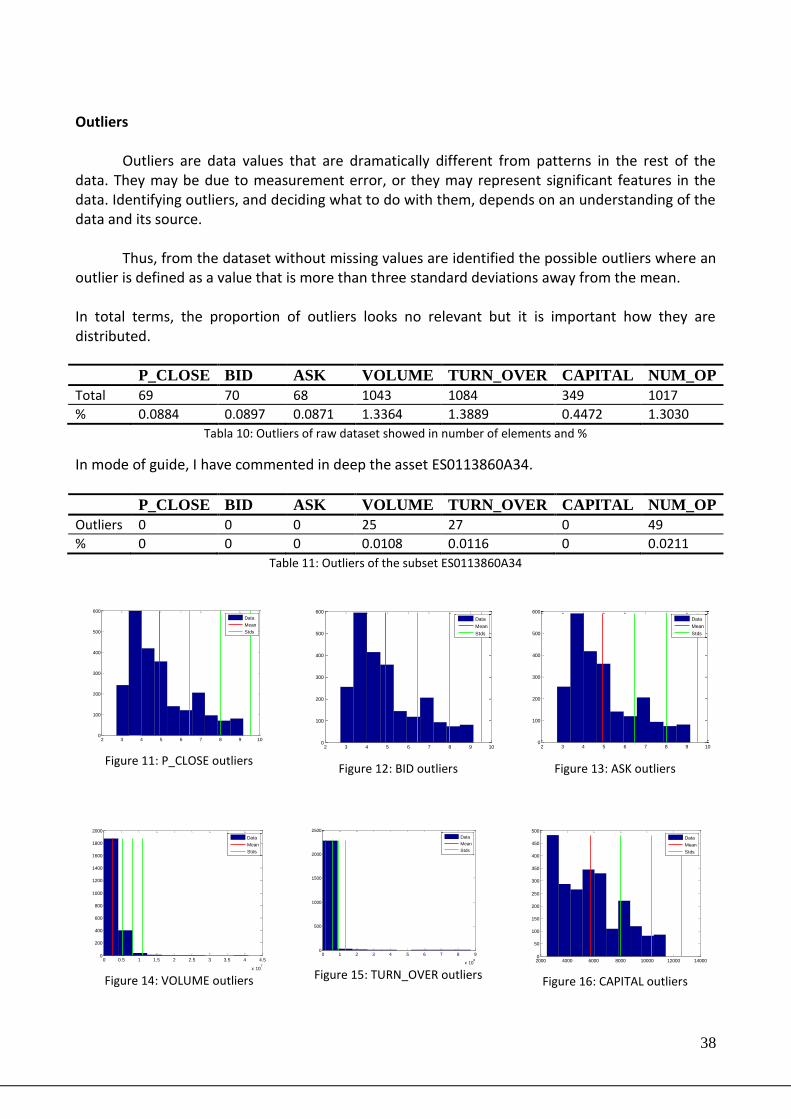


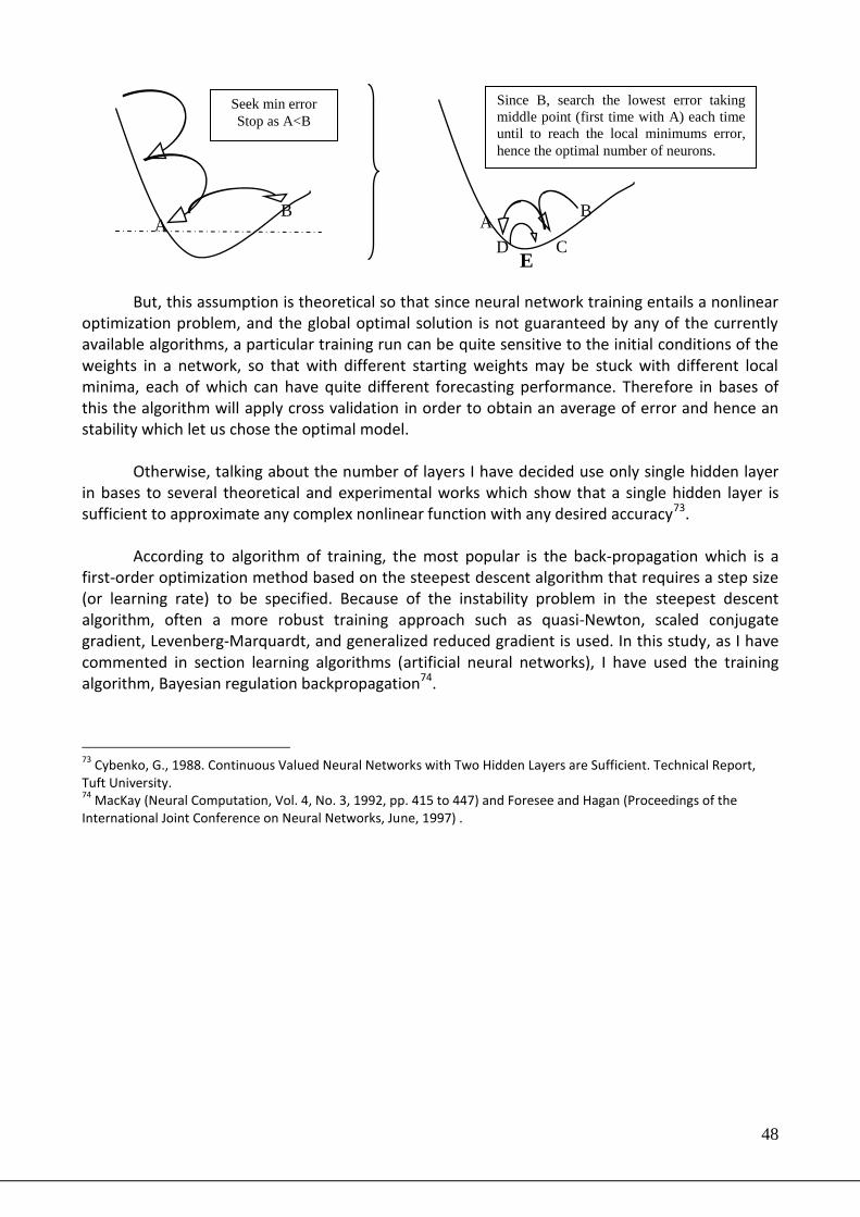


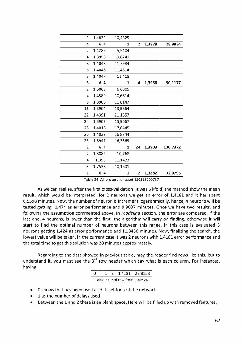


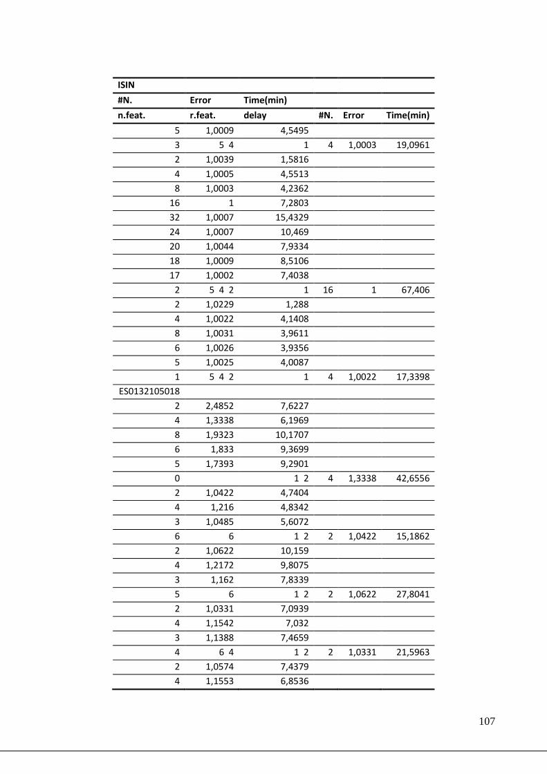


![(d, ,]) Fuzzy Logic - UPCommons](https://static.documents.pub/doc/80x56/6207321549d709492c2ee10d/d-fuzzy-logic-upcommons.jpg)