Page 1
ABSTRACT
MOHAMED, ISMAIL. Sensitivity Analysis of the Applied Element Method for the
Buckling of Uni-axially Compressed Plates. (Under the direction of committee chair Dr.
Robert White.)
The Applied Element Method (AEM) is a numerical method, like the Finite Element
Method. The AEM discretizes the domain into a grid of rigid finite elements with the degrees
of freedom, three translations and three rotations, located in the geometric center of the
element. The connection of the elements is established through a mesh of springs on the
contact faces of the elements. To study the accuracy of the AEM, a plate buckling problem is
selected. The study drives the governing differential equation for the buckling of this plate
under a simply supported (Dirichlet and Neumann) boundary conditions. Then the theoretical
solution is presented as infinite sum of double trigonometric series and hence the minimum
buckling load and the corresponding buckling mode are calculated. Then we build the
discrete model using the AEM and find the numerical solution for three different parameters;
the element size, the spring distribution and the Shear stiffness. The method converges with
increasing the number of the springs and with decreasing the element size when the proper
estimation of the shear stiffness is used. To study the effect of the shear stiffness, a new
correction has been introduced to account for the element size ratio on the spring shear
stiffness when solving thin plates or thin walled structures in general. The correction seems
to perform accurately for some element sizes. It is recommended that further studies should
be done to find estimation for the shear stiffness.
Page 2
© Copyright 2013 by Ismail Mohamed
All Rights Reserved
Page 3
Sensitivity Analysis of the Applied Element Method for the Buckling of Uni-axially
compressed Plates
by
Ismail Mohamed
A thesis submitted to the Graduate Faculty of
North Carolina State University
in partial fulfillment of the
requirements for the degree of
Master of Science
Applied Mathematics
Raleigh, North Carolina
2013
APPROVED BY:
______________________________ ______________________________
Dr. Ernest Stitzinger Dr. Zhilin Li
________________________________
Dr. Robert White
Chair of Advisory Committee
Page 4
ii
BIOGRAPHY
Ismail Mohamed attended Cairo University in Egypt as an undergraduate student. He
obtained his Bachelors of Science in Civil Engineering in 1998. He continued his graduate
studies while he was working in the private sector. He got his Master of Science in Structural
engineering in 2004. After working for the private sector for some years in the USA, he
joined the North Carolina State University for the degree of Doctor of Philosophy in
Structural engineering and a Master degree in Applied Mathematics.
Page 5
iii
ACKNOWLEDMENTS
I would like to express my sincere gratitude to Dr. White for his support and
dedication in this research. I would like also to thank Dr. Stitzinger and Dr. Li to serve in the
examining committee and their valuable comments. I would like to acknowledge the Applied
Science International for providing the Extreme Loading for Structures Software to perform
this study.
Page 6
iv
TABLE OF CONTENTS
LIST OF TABLES ................................................................................................................... vi
LIST OF FIGURES ................................................................................................................ vii
CHAPTER 1 INTRODUCTION .............................................................................................. 1
1.1 Motivation and Objectives ........................................................................................ 1
1.2 Overview of the contents of the Thesis .................................................................... 3
CHAPTER 2 Buckling of Plates ............................................................................................... 4
2.1 Introduction ............................................................................................................... 4
2.2 Derivation of the Governing Equation ...................................................................... 7
2.3 Boundary Conditions .............................................................................................. 11
2.4 Solution of the governing equation ......................................................................... 12
CHAPTER 3 The Applied Element Method .......................................................................... 16
3.1 Introduction ............................................................................................................. 16
3.2 AEM Formulation ................................................................................................... 17
3.3 AEM Verification ................................................................................................... 20
CHAPTER 4 RESULTS and DISCUSSION .......................................................................... 23
4.1 Introduction ............................................................................................................. 23
4.2 Problem Set-up ....................................................................................................... 23
4.3 AEM Model ............................................................................................................ 24
4.4 Numerical Results ................................................................................................... 26
4.4.1 Effect of the number of springs .......................................................................... 26
4.4.2 Effect of the shear modulus G ............................................................................ 27
4.4.3 Effect of the element size .................................................................................... 27
Page 7
v
4.5 Discussion of the Numerical Results ...................................................................... 27
4.5.1 Effect of the correction to the shear modulus G ................................................. 28
4.5.2 Comparison of the correction to the shear modulus G with the exact value ...... 28
CHAPTER 5 CONCLUSIONS AND FUTURE WORK ....................................................... 35
5.1 Conclusions ............................................................................................................. 35
5.2 Future Work ............................................................................................................ 36
REFERENCES ....................................................................................................................... 37
Page 8
vi
LIST OF TABLES
Table 4-1: Testing Values for the shear modulus, element size and springs distribution. ..... 29
Table 4-2: The buckling load for element size 10 (mm) for different spring distribution
and different G values. ............................................................................................................ 30
Table 4-3: The relative error of the buckling load for element size 10 (mm) for different
spring distribution and different G values. ............................................................................. 30
Table 4-4: Interpolation of the G values compared with the proposed correction values. .... 30
Page 9
vii
LIST OF FIGURES
Figure 1-1: AEM Mesh. ........................................................................................................... 2
Figure 2-1: Local buckling of compression elements. (a) Beams. (b) Column. adopted
from (Yu 2000) ......................................................................................................................... 5
Figure 2-2: Load versus Out-of-plane Displacement .............................................................. 6
Figure 2-3: Forces and moments of the differential element. .................................................. 8
Figure 2-4: Rectangular plate subjected to uni-axial compression stress. ............................. 13
Figure 2-5: Buckling factor versus plate aspect ratio for simply supported rectangular
plate. ........................................................................................................................................ 15
Figure 3-1: Advantages of AEM. .......................................................................................... 17
Figure 3-2: Spring representative area. .................................................................................. 19
Figure 3-3: Degrees of freedom and end forces of two elements, (a) Idealized position,
(b) General position. ............................................................................................................... 19
Figure 3-4: Example 1 Set up. ............................................................................................... 20
Figure 3-5: Example 1 Results............................................................................................... 21
Figure 3-6: Example 2 Set up and Results. ............................................................................ 21
Figure 3-7: Example 3 Set up and results. ............................................................................. 22
Figure 4-1: Plate dimensions, boundary conditions and loading. .......................................... 24
Figure 4-2: Typical plate mesh, boundary conditions and loading. ....................................... 25
Figure 4-3: Typical plate results; left: the buckling mode and right: the load-
displacement chart. ................................................................................................................. 25
Figure 4-4: Effect of number of springs for different values of G and for element size 10
mm. ......................................................................................................................................... 31
Figure 4-5: Effect of number of springs for different values of G and for element size 10
mm as a relative error. ............................................................................................................ 31
Page 10
viii
Figure 4-6: effect of the shear modulus (G) for different values of spring distribution and
for element size 10 mm. .......................................................................................................... 32
Figure 4-7: Effect of the element size for different values of G and for 5 by 5 spring
distribution. ............................................................................................................................. 32
Figure 4-8: Effect of the element size for different values of G and for 5 by 5 spring
distribution relative error. ....................................................................................................... 33
Figure 4-9: Effect of the element size for different spring distribution using the G
correction factor. ..................................................................................................................... 33
Figure 4-10: Effect of the element size for different spring distribution using the G
correction factor, relative error. .............................................................................................. 34
Figure 4-11: The ratio of the Exact and corrected shear modulus versus element ratio. ....... 34
Page 11
1
CHAPTER 1
INTRODUCTION
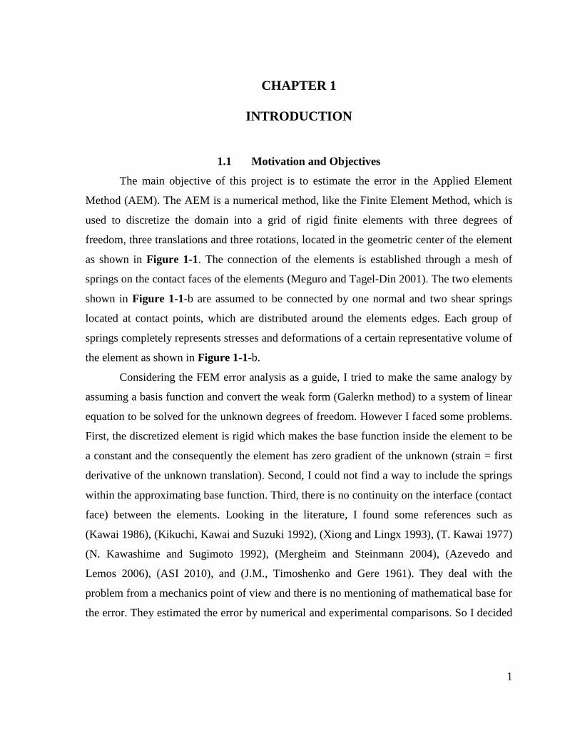
1.1 Motivation and Objectives
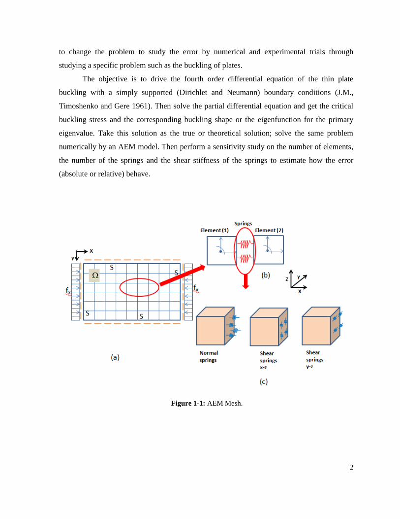
The main objective of this project is to estimate the error in the Applied Element
Method (AEM). The AEM is a numerical method, like the Finite Element Method, which is
used to discretize the domain into a grid of rigid finite elements with three degrees of
freedom, three translations and three rotations, located in the geometric center of the element
as shown in Figure 1-1. The connection of the elements is established through a mesh of
springs on the contact faces of the elements (Meguro and Tagel-Din 2001). The two elements
shown in Figure 1-1-b are assumed to be connected by one normal and two shear springs
located at contact points, which are distributed around the elements edges. Each group of
springs completely represents stresses and deformations of a certain representative volume of
the element as shown in Figure 1-1-b.
Considering the FEM error analysis as a guide, I tried to make the same analogy by
assuming a basis function and convert the weak form (Galerkn method) to a system of linear
equation to be solved for the unknown degrees of freedom. However I faced some problems.
First, the discretized element is rigid which makes the base function inside the element to be
a constant and the consequently the element has zero gradient of the unknown (strain = first
derivative of the unknown translation). Second, I could not find a way to include the springs
within the approximating base function. Third, there is no continuity on the interface (contact
face) between the elements. Looking in the literature, I found some references such as
(Kawai 1986), (Kikuchi, Kawai and Suzuki 1992), (Xiong and Lingx 1993), (T. Kawai 1977)
(N. Kawashime and Sugimoto 1992), (Mergheim and Steinmann 2004), (Azevedo and
Lemos 2006), (ASI 2010), and (J.M., Timoshenko and Gere 1961). They deal with the
problem from a mechanics point of view and there is no mentioning of mathematical base for
the error. They estimated the error by numerical and experimental comparisons. So I decided
Page 12
2
to change the problem to study the error by numerical and experimental trials through
studying a specific problem such as the buckling of plates.
The objective is to drive the fourth order differential equation of the thin plate
buckling with a simply supported (Dirichlet and Neumann) boundary conditions (J.M.,
Timoshenko and Gere 1961). Then solve the partial differential equation and get the critical
buckling stress and the corresponding buckling shape or the eigenfunction for the primary
eigenvalue. Take this solution as the true or theoretical solution; solve the same problem
numerically by an AEM model. Then perform a sensitivity study on the number of elements,
the number of the springs and the shear stiffness of the springs to estimate how the error
(absolute or relative) behave.
Figure 1-1: AEM Mesh.
Page 13
3
1.2 Overview of the contents of the Thesis
Chapter 2 presents a discussion of the derivation of the governing differential
equation of the plate buckling then solves the theoretical solution of the minimum buckling
value and the corresponding mode shape. Chapter 3 describes the Applied Element method
formulation and shows some verification examples compared with the experiments. Chapter
4 presents the study of three parameters on obtaining the buckling load. The three parameters
are; the element size, the spring distribution and the shear stiffness of the spring. Chapter 5
summarizes the main conclusions and future work.
Page 14
4
CHAPTER 2
BUCKLING OF PLATES
2.1 Introduction
Flat plates are extensively used in many engineering applications like roof and floor
of buildings, deck slab of bridges, foundation footings, water tanks, bulk heads, etc. Plate
buckling governs the design of many types of structures, for example, the thickness of the
walls used in thin-wall beams. The most efficient designs, used for large spans, usually
employ stiffness plates. For purpose of stability analysis, the wall plates between stiffening
ribs may normally be analyzed approximately as isolated rectangular plates (Bazant 1991). In
cold-formed steel design, individual elements of cold-formed steel structural members are
usually thin and the width-to-thickness ratios are large (Yu 2000). These thin elements may
buckle locally at a stress level lower than the yield point of steel when they are subject to
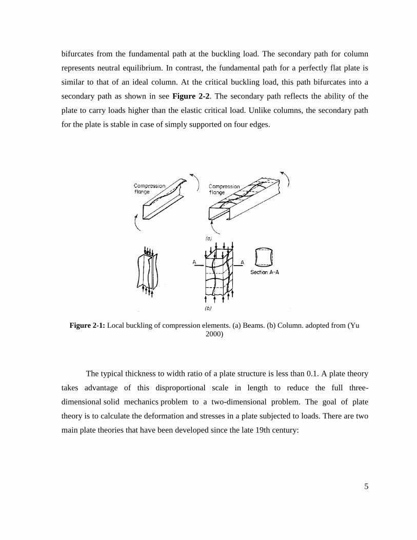
compression in flexural bending, axial compression, shear, or bearing. Figure 2-1 illustrates
local buckling patterns of certain beams and columns, where the line junctions between
elements remain straight and angles between elements do not change.
The plates used in these applications are usually loaded either in-plane which causes
buckling or out of plane, lateral, which causes bending. The geometry of the plate is normally
defined by the middle plane which is a plane equidistant from the top and bottom faces of the
plate. The thickness of the plate (t) is measured in a direction normal to the middle plane of
the plate. The flexural properties of the plate largely depend on its thickness rather than its
other two dimensions (length and width).
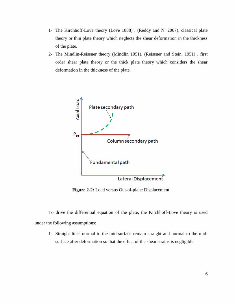
The plate buckling is different than the common known column buckling. In case of
an ideal column, as the axial load is increased, the lateral displacement remains zero until the
reaching the critical buckling load (Euler load). If we plot the axial load versus lateral
displacement, we will get a line along the load axis up to P = Pcr, see Figure 2-2. This is
called the fundamental path. When the axial load equals to the Euler buckling load the lateral
displacement increases indefinitely at constant load. This is the secondary path, which
Page 15
5
bifurcates from the fundamental path at the buckling load. The secondary path for column
represents neutral equilibrium. In contrast, the fundamental path for a perfectly flat plate is
similar to that of an ideal column. At the critical buckling load, this path bifurcates into a
secondary path as shown in see Figure 2-2. The secondary path reflects the ability of the
plate to carry loads higher than the elastic critical load. Unlike columns, the secondary path
for the plate is stable in case of simply supported on four edges.
Figure 2-1: Local buckling of compression elements. (a) Beams. (b) Column. adopted from (Yu
2000)
The typical thickness to width ratio of a plate structure is less than 0.1. A plate theory
takes advantage of this disproportional scale in length to reduce the full three-
dimensional solid mechanics problem to a two-dimensional problem. The goal of plate
theory is to calculate the deformation and stresses in a plate subjected to loads. There are two
main plate theories that have been developed since the late 19th century:
Page 16
6
1- The Kirchhoff-Love theory (Love 1888) , (Reddy and N. 2007), classical plate
theory or thin plate theory which neglects the shear deformation in the thickness
of the plate.
2- The Mindlin-Reissner theory (Mindlin 1951), (Reissner and Stein. 1951) , first
order shear plate theory or the thick plate theory which considers the shear
deformation in the thickness of the plate.
Figure 2-2: Load versus Out-of-plane Displacement
To drive the differential equation of the plate, the Kirchhoff-Love theory is used
under the following assumptions:
1- Straight lines normal to the mid-surface remain straight and normal to the mid-
surface after deformation so that the effect of the shear strains is negligible.
Page 17
7
2- The normal stress and the corresponding normal strain in the normal plane to the
mid-surface are negligible for very small deflection ration of the plate span
because it’s a small deformation analysis.
3- The plate is ideally flat and the thickness of the plate does not change during a
deformation.
4- All loads do not change magnitude or direction when the plate buckles. All
applied loads strictly acting in the middle plane of the plate.
5- The material is homogeneous, isotropic, continuous, and linearly elastic.
2.2 Derivation of the Governing Equation
Drive model Eq. 2-21 and the BVP Eq. 2-25 are adopted from (Gambhir 2004).
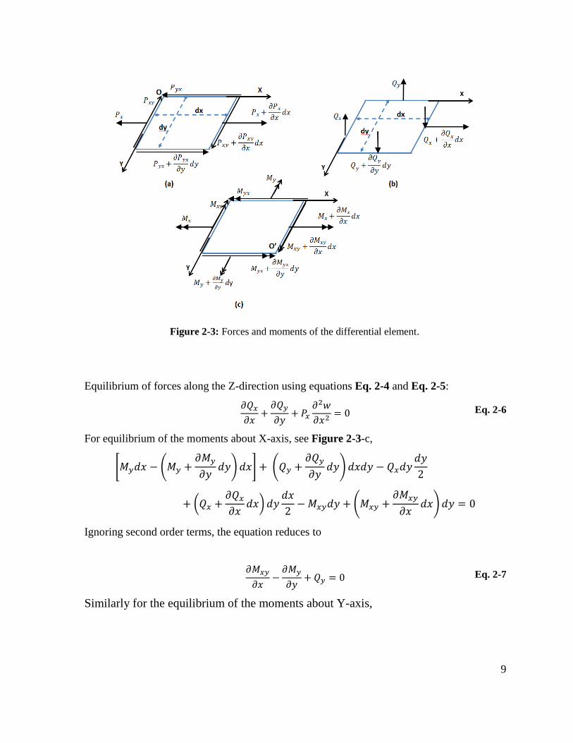
Consider an initial state of equilibrium of a rectangular plate of dimensions a and b such that
a >> b subjected to the external edge loads acting in the middle plane of the plate. And
consider a free body of a rectangular differential element cut away from that plate with
dimensions dx, dy, and t as shown in Figure 2-3-a. The governing differential equation is
obtained from the static equilibrium equation of the deformed shape, namely.
∑ ∑ ∑ ∑ Eq. 2-1
Consider the equilibrium of in-plane forces in X-direction as shown in Figure 2-3-a
∑ (
) (
)
Eq. 2-2
Equilibrium of the moments of in-plane forces about Z-axis passing through O’ and
after ignoring the second order terms, yields,
∑ (
)
Eq. 2-3
Page 18
8
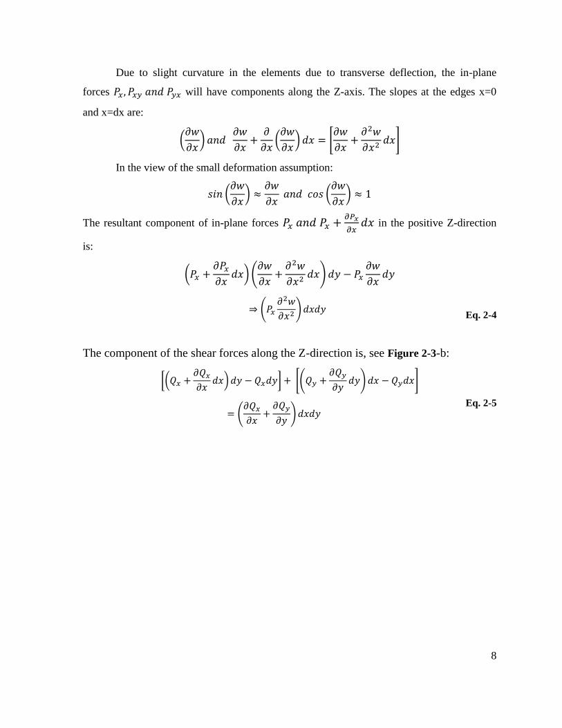
Due to slight curvature in the elements due to transverse deflection, the in-plane
forces will have components along the Z-axis. The slopes at the edges x=0
and x=dx are:
(
)
(
) [
]
In the view of the small deformation assumption:
(
)
(
)
The resultant component of in-plane forces
in the positive Z-direction
is:
(
) (
)
(
)
Eq. 2-4
The component of the shear forces along the Z-direction is, see Figure 2-3-b:
[(
) ] [(
) ]
(
)
Eq. 2-5
Page 19
9
Figure 2-3: Forces and moments of the differential element.
Equilibrium of forces along the Z-direction using equations Eq. 2-4 and Eq. 2-5:
Eq. 2-6
For equilibrium of the moments about X-axis, see Figure 2-3-c,
[ (
) ] (
)
(
)
(
)
Ignoring second order terms, the equation reduces to
Eq. 2-7
Similarly for the equilibrium of the moments about Y-axis,
Page 20
10
Eq. 2-8
From Eq. 2-7 and Eq. 2-8,
Eq. 2-9
Eq. 2-10
Substituting from equations Eq. 2-10 and Eq. 2-9 respectively into
equation Eq. 2-6,
Eq. 2-11
This last equation is the governing differential equation of buckling of plates. The
moments in the equation can be expressed in terms of the curvatures. Since a thin plate is
essentially two dimensional, the constitutive law for an elastic plane-stress problem can be
used. These are:
( )
( )
Eq. 2-12
The strain-displacement relations for a linear problem expressed as
Eq. 2-13
Let u and be the displacement along X and Y directions at a distance z above the
middle surface which remains unstrained during the transverse displacement, , thus
Eq. 2-14
Hence the strains can be represented by
Page 21
11
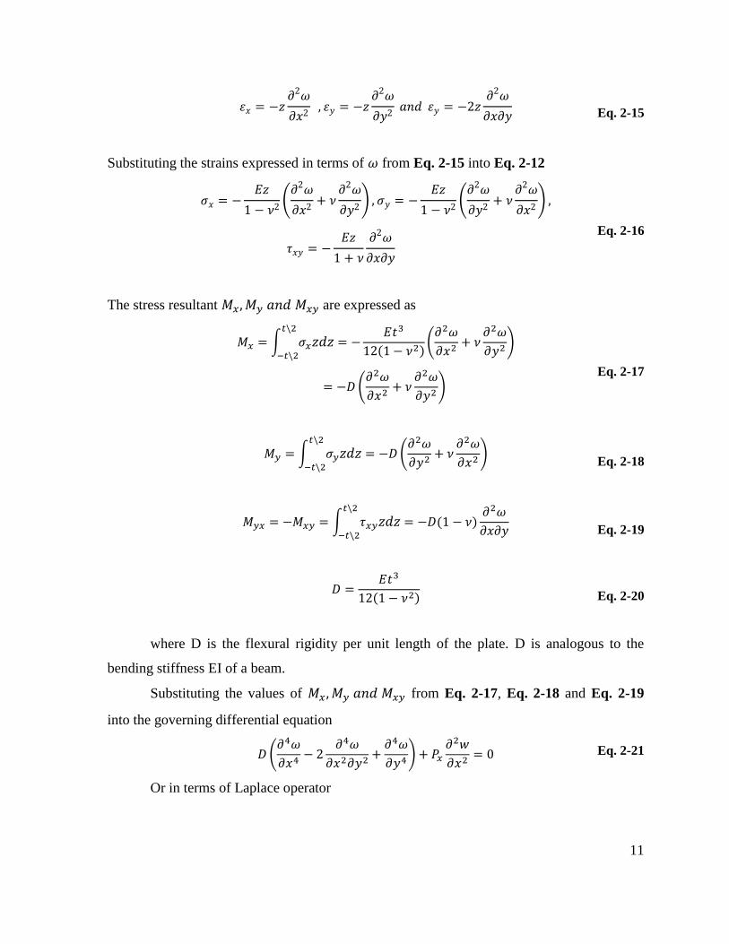
Eq. 2-15
Substituting the strains expressed in terms of from Eq. 2-15 into Eq. 2-12
(
)
(
)
Eq. 2-16
The stress resultant are expressed as
∫
(
)
(
)
Eq. 2-17
∫
(
)
Eq. 2-18
∫
Eq. 2-19
Eq. 2-20
where D is the flexural rigidity per unit length of the plate. D is analogous to the
bending stiffness EI of a beam.
Substituting the values of from Eq. 2-17, Eq. 2-18 and Eq. 2-19
into the governing differential equation
(
)
Eq. 2-21
Or in terms of Laplace operator
Page 22
12
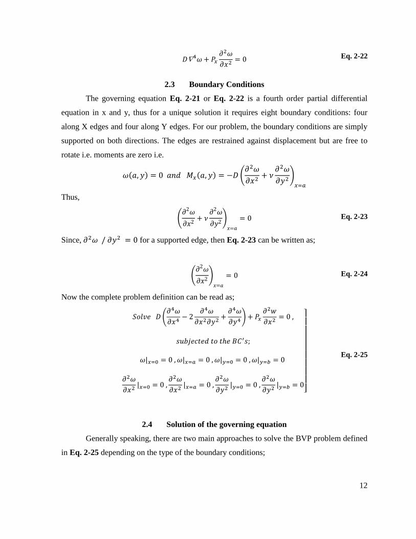
Eq. 2-22
2.3 Boundary Conditions
The governing equation Eq. 2-21 or Eq. 2-22 is a fourth order partial differential
equation in x and y, thus for a unique solution it requires eight boundary conditions: four
along X edges and four along Y edges. For our problem, the boundary conditions are simply
supported on both directions. The edges are restrained against displacement but are free to
rotate i.e. moments are zero i.e.
(
)
Thus,
(
)
Eq. 2-23
Since, for a supported edge, then Eq. 2-23 can be written as;
(
)
Eq. 2-24
Now the complete problem definition can be read as;
(
)
]
Eq. 2-25
2.4 Solution of the governing equation
Generally speaking, there are two main approaches to solve the BVP problem defined
in Eq. 2-25 depending on the type of the boundary conditions;
Page 23
13
1- Navier solution which assumes the solution as the infinite sum of double series. It
can account for any type of loading but limited to only all-round simply supported
rectangular plate.
2- Levy solution which is a more general solution and requires only one pair of
edges (opposite edges) to be simply supported while the other pair can have any
type of boundary conditions. The solution is assumed as a two parts, the
homogeneous part and the particular part.
The Navier solution is used to obtain the exact buckling load and mode shape. The deflected
shape of the rectangular plate shown in Figure 2-4 may be represented by a double
trigonometric series
∑ ∑
(
) (
) Eq. 2-26
Where, m and n are the number of half sine waves in the x and y directions, respectively.
Obviously, satisfy the boundary conditions in Eq. 2-25 since sin(0) = sin( ) = 0 at x = 0,a
and y = 0,b. Substituting Eq. 2-26 into Eq. 2-25 to obtain,
∑ ∑
[ (
)
] (
) (
) Eq. 2-27
One of the solutions is which makes and hence there is no buckling which
corresponds to the unloaded case. The other solution is
Figure 2-4: Rectangular plate subjected to uni-axial compression stress.
Page 24
14
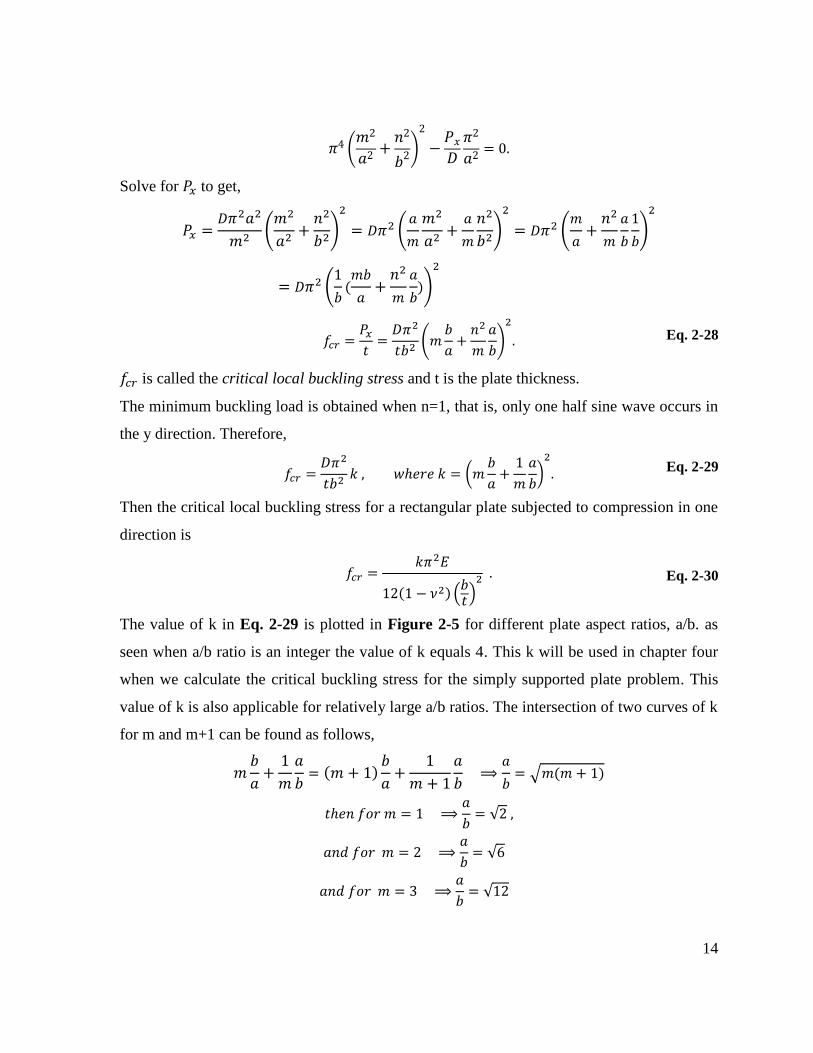
(
)
Solve for to get,
(
)
(
)
(
)
(
)
(
)
Eq. 2-28
is called the critical local buckling stress and t is the plate thickness.
The minimum buckling load is obtained when n=1, that is, only one half sine wave occurs in
the y direction. Therefore,
(
)
Eq. 2-29
Then the critical local buckling stress for a rectangular plate subjected to compression in one
direction is
( )
Eq. 2-30
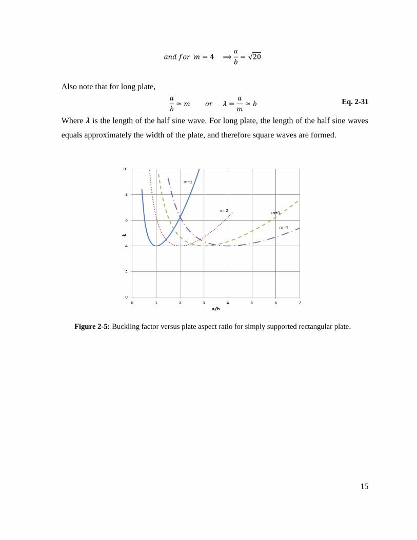
The value of k in Eq. 2-29 is plotted in Figure 2-5 for different plate aspect ratios, a/b. as
seen when a/b ratio is an integer the value of k equals 4. This k will be used in chapter four
when we calculate the critical buckling stress for the simply supported plate problem. This
value of k is also applicable for relatively large a/b ratios. The intersection of two curves of k
for m and m+1 can be found as follows,
√
√
√
√
Page 25
15
√
Also note that for long plate,
Eq. 2-31
Where is the length of the half sine wave. For long plate, the length of the half sine waves
equals approximately the width of the plate, and therefore square waves are formed.
Figure 2-5: Buckling factor versus plate aspect ratio for simply supported rectangular plate.
Page 26
16
CHAPTER 3
THE APPLIED ELEMENT METHOD
3.1 Introduction
Since the introducing of the computers in the scientific and engineering research in
the second half of the nineteenth century, many numerical techniques have been developed to
solve bigger and more complex structures. Numerical methods took two main directions
based on the nature of the discretization of the continuous domain. Methods that discretize
the domain into elements which can deform such as the Finite element Method and methods
that discretize the domain into elements which are rigid, no deformations inside the element
such as the Discrete Element Method or the Rigid Body and Spring Model (Kawai 1986).
The main advantage of the latter is the simplicity to separate the elements. However the main
disadvantage is the crack propagation depends on the mesh shape and size (Kikuchi, Kawai
and Suzuki 1992). The Applied Element Method (AEM) is one of the discrete element
methods.
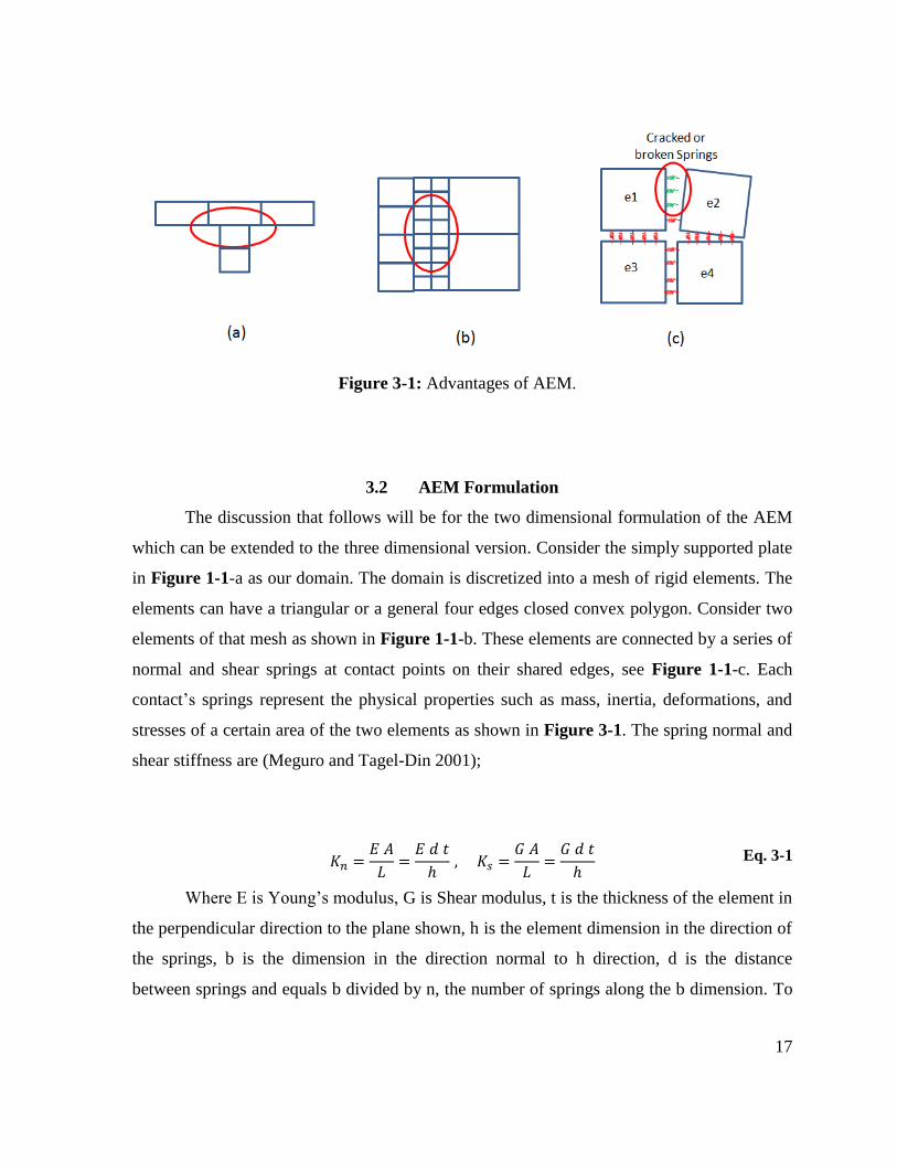
The main advantages of AEM are (Meguro and Tagel-Din 2001):
1- Element connectivity is through faces not nodes. So it’s very normal to have
elements connected as shown in Figure 3-1-a.
2- There is no need for transition elements to connect elements of different
geometry, see Figure 3-1-b.
3- It’s very simple to break or crack the element connectivity by removing the
springs. The degrees of freedom are at the nodes inside the elements. There are no
nodes to break as in case of the Finite Element Method as shown in Figure 3-1-c.
4- There is no need to develop special element for interface between the elements as
in the case of the Finite Element Method. The springs are already in the interface
mode by default. Any spring can represent any path-dependent constitutive laws
of the material as shown in Figure 3-1-b.
Page 27
17
Figure 3-1: Advantages of AEM.
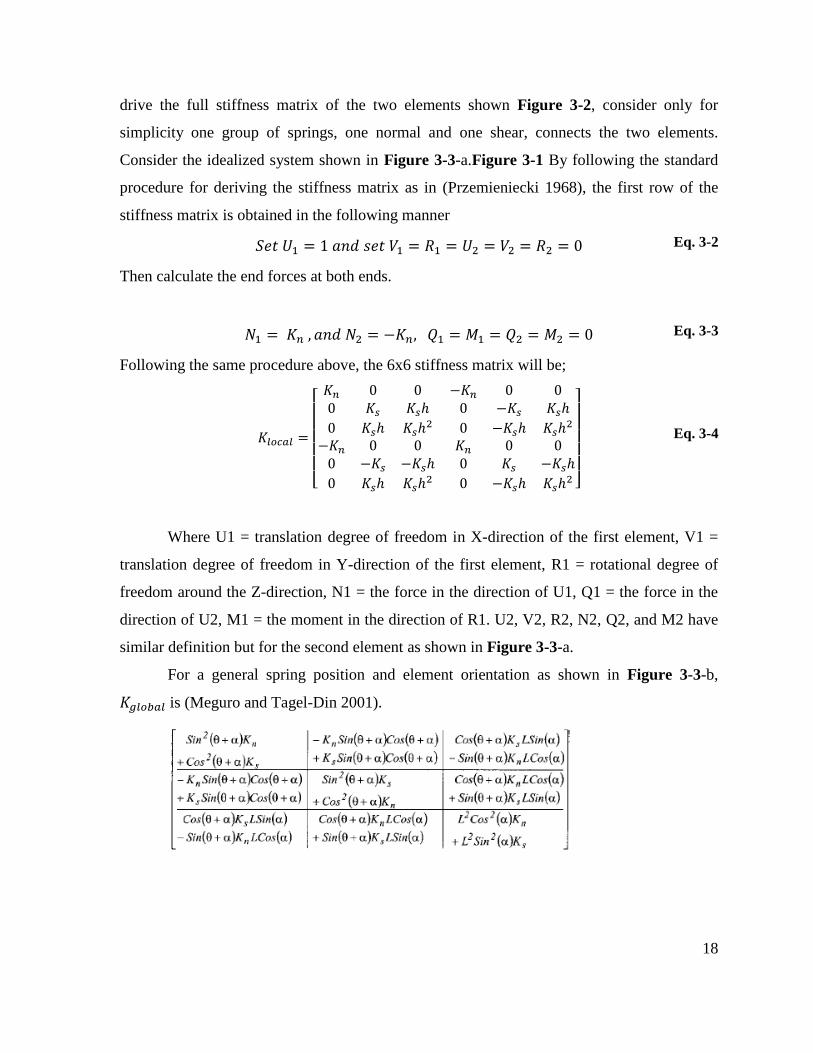
3.2 AEM Formulation
The discussion that follows will be for the two dimensional formulation of the AEM
which can be extended to the three dimensional version. Consider the simply supported plate
in Figure 1-1-a as our domain. The domain is discretized into a mesh of rigid elements. The
elements can have a triangular or a general four edges closed convex polygon. Consider two
elements of that mesh as shown in Figure 1-1-b. These elements are connected by a series of
normal and shear springs at contact points on their shared edges, see Figure 1-1-c. Each
contact’s springs represent the physical properties such as mass, inertia, deformations, and
stresses of a certain area of the two elements as shown in Figure 3-1. The spring normal and
shear stiffness are (Meguro and Tagel-Din 2001);
Eq. 3-1
Where E is Young’s modulus, G is Shear modulus, t is the thickness of the element in
the perpendicular direction to the plane shown, h is the element dimension in the direction of
the springs, b is the dimension in the direction normal to h direction, d is the distance
between springs and equals b divided by n, the number of springs along the b dimension. To
Page 28
18
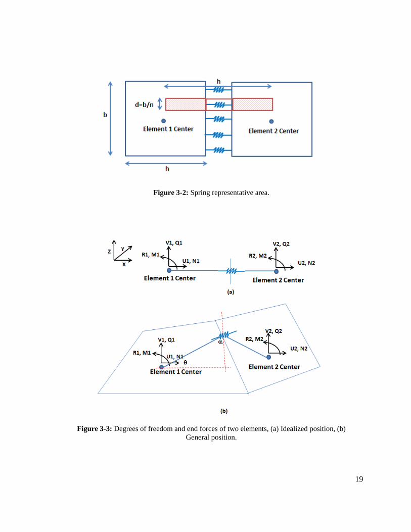
drive the full stiffness matrix of the two elements shown Figure 3-2, consider only for
simplicity one group of springs, one normal and one shear, connects the two elements.
Consider the idealized system shown in Figure 3-3-a.Figure 3-1 By following the standard
procedure for deriving the stiffness matrix as in (Przemieniecki 1968), the first row of the
stiffness matrix is obtained in the following manner
Eq. 3-2
Then calculate the end forces at both ends.
Eq. 3-3
Following the same procedure above, the 6x6 stiffness matrix will be;
[
]
Eq. 3-4
Where U1 = translation degree of freedom in X-direction of the first element, V1 =
translation degree of freedom in Y-direction of the first element, R1 = rotational degree of
freedom around the Z-direction, N1 = the force in the direction of U1, Q1 = the force in the
direction of U2, M1 = the moment in the direction of R1. U2, V2, R2, N2, Q2, and M2 have
similar definition but for the second element as shown in Figure 3-3-a.
For a general spring position and element orientation as shown in Figure 3-3-b,
is (Meguro and Tagel-Din 2001).
Page 29
19
Figure 3-2: Spring representative area.
Figure 3-3: Degrees of freedom and end forces of two elements, (a) Idealized position, (b)
General position.
Page 30
20
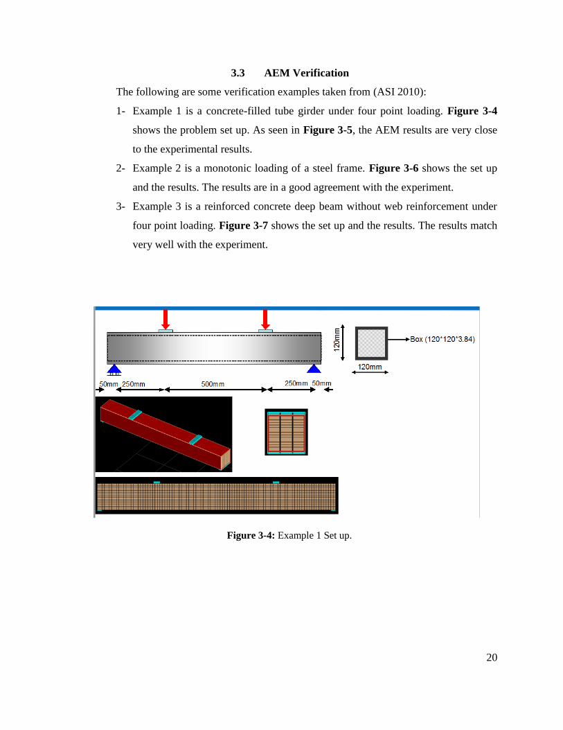
3.3 AEM Verification
The following are some verification examples taken from (ASI 2010):
1- Example 1 is a concrete-filled tube girder under four point loading. Figure 3-4
shows the problem set up. As seen in Figure 3-5, the AEM results are very close
to the experimental results.
2- Example 2 is a monotonic loading of a steel frame. Figure 3-6 shows the set up
and the results. The results are in a good agreement with the experiment.
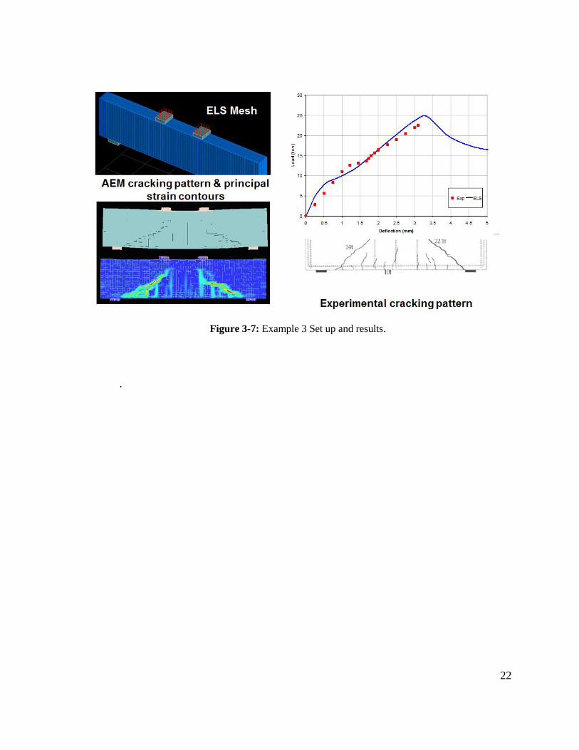
3- Example 3 is a reinforced concrete deep beam without web reinforcement under
four point loading. Figure 3-7 shows the set up and the results. The results match
very well with the experiment.
Figure 3-4: Example 1 Set up.
Page 31
21
Figure 3-5: Example 1 Results.
Figure 3-6: Example 2 Set up and Results.
Page 32
22
Figure 3-7: Example 3 Set up and results.
.
Page 33
23
CHAPTER 4
RESULTS AND DISCUSSION
4.1 Introduction
This chapter is devoted to study the effect of some parameters on the accuracy of the
AEM, namely; the number of elements, the number of springs and the value of the shear
modulus. The model problem used here is the buckling of the uni-axiallly compressed
rectangular plate whose theoretical solution was discussed in chapter 2. The strategy is to
build an experimental matrix of runs or simulations. The matrix contains more than 300 runs.
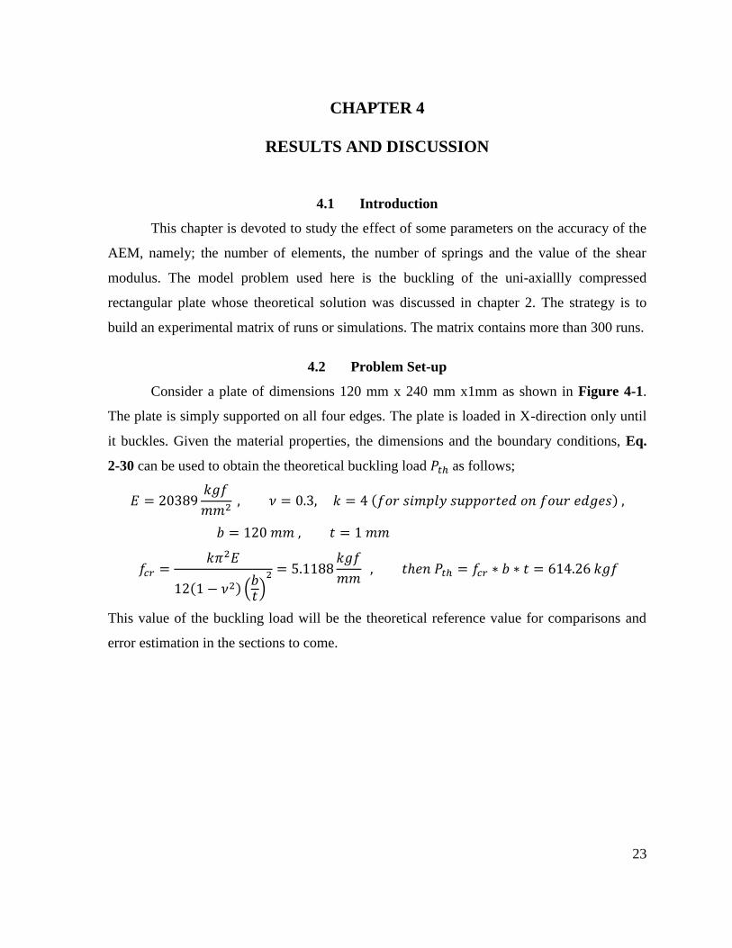
4.2 Problem Set-up
Consider a plate of dimensions 120 mm x 240 mm x1mm as shown in Figure 4-1.
The plate is simply supported on all four edges. The plate is loaded in X-direction only until
it buckles. Given the material properties, the dimensions and the boundary conditions, Eq.
2-30 can be used to obtain the theoretical buckling load as follows;
( )
This value of the buckling load will be the theoretical reference value for comparisons and
error estimation in the sections to come.
Page 34
24
Figure 4-1: Plate dimensions, boundary conditions and loading.
4.3 AEM Model
Figure 4-2 shows the AEM model. The AEM is implemented in the Extreme Loading
for Structures software (ELS®) produced by the Applied Science International (ASI) Inc.
The ELS is used to build and run the models. The plate model is lying in the x-y plane. The
boundary conditions were applied at the center of the element. The figure also shows the
spring distribution on the element faces. The elements were loaded in the X-direction with an
incremental controlled displacement of 0.000035 mm per increment to ensure a very slow
load progression to capture the minimum buckling load. The mesh discretization is kept one
element in the thickness direction. The element size is kept as square in the x-y plane with
the number of elements in the X-direction is always twice the number of elements in the Y-
direction. Figure 4-3 shows a typical output of running one of the models. As it’s shown on
the left, the buckling mode matches the differential equation solution discussed in chapter
two. Since the length in the X-directions is twice the length in the Y-direction, there is a
double half sine wave in the X-direction while there is only one half sine wave in the Y-
direction. The right half of the same figure shows a typical load versus displacement curve.
As discussed in the introduction in chapter two, the plate buckling takes the fundamental
paths then bifurcates in a stable secondary path where it can still carry more load beyond the
critical buckling load.
Page 35
25
Figure 4-2: Typical plate mesh, boundary conditions and loading.
Figure 4-3: Typical plate results; left: the buckling mode and right: the load-displacement
chart.
Page 36
26
4.4 Numerical Results
Table 4-1shows the list of values for the three studied parameters;
1- Shear Modulus, G is presented as a multiple of the Young’s modulus. The shear
stiffness of the spring was presented in chapter two as Ks=GA/L. When trying
this value in the simulation, the error in obtaining the buckling was very high
compared to the theoretical value. Upon trying different values for shear stiffness,
it was found that this change can give very good results. But the question is how
to get this value and what is the theory behind it. To study this effect, the shear
stiffness is added as another parameter in the experimental matrix. As a user to
the ELS software, the only way to change the shear stiffness was to factor the
shear modulus to account for the desired change. So it was selected to represent
the G as a multiple of the E in the study.
2- The element size was chosen to range from ten times the thickness (1/10) to one
times the thickness (1/1). The element dimensions are kept as a square in the xy-
plane.
3- The spring distribution ranges from 2 by 2 springs on the shared faces of the
elements to 20 by 20.
For every element size, a table like the one in Table 4-2 was built by running all these
simulations. This table shows the buckling load using different combination of G and springs
distribution. Table 4-3 shows the relative error of the results of Table 4-2. The relative error
is defined as where is the theoretical buckling load calculated in the
previous sections and is the numerical buckling load using the AEM.
4.4.1 Effect of the number of springs
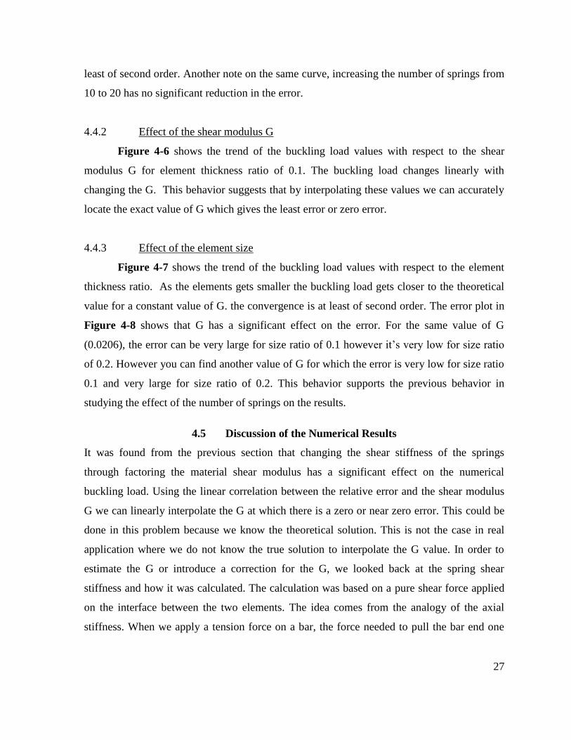
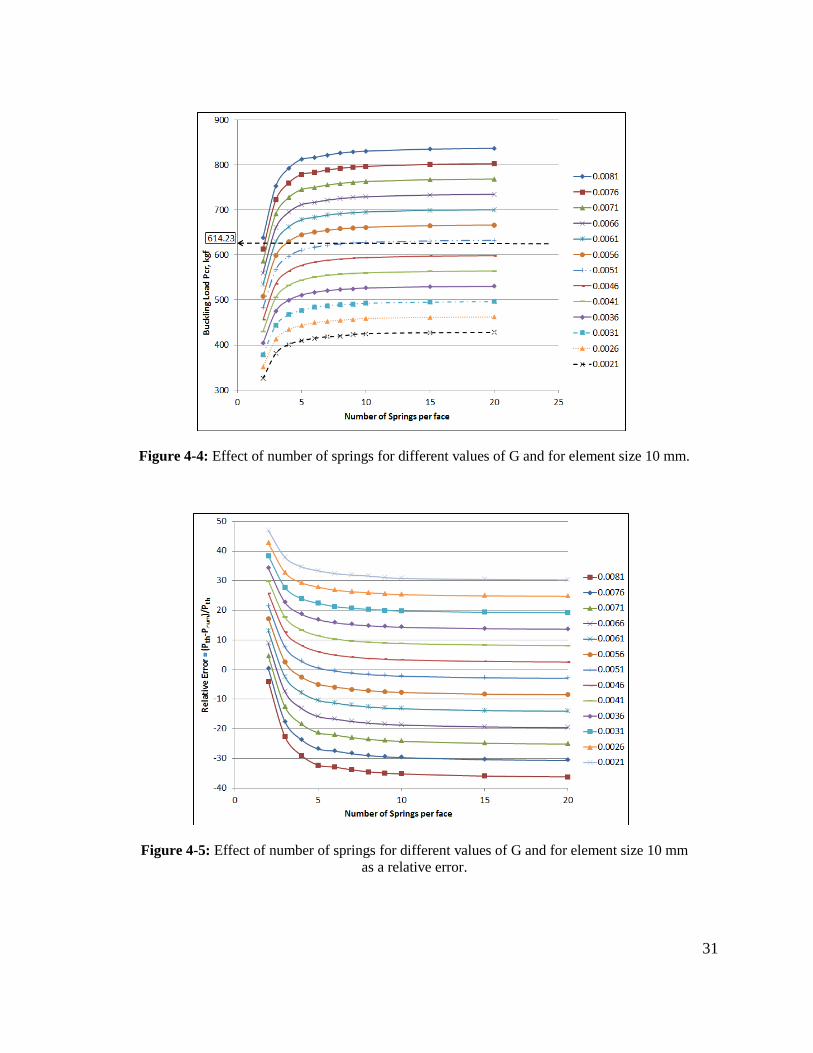
Figure 4-4 shows the plot of the data of Table 4-2. For any single value of G, as the
number of springs increases, the buckling load gets closer and closer to the theoretical value.
It’s worth mentioning that increasing the number of springs from 2 by 2 to 5 by 5 reduces the
error significantly from 20% to less than 1% as shown in Figure 4-4 when G = 0.0051. The
curve suggests that the convergence of the method with respect to the number of springs is at
Page 37
27
least of second order. Another note on the same curve, increasing the number of springs from
10 to 20 has no significant reduction in the error.
4.4.2 Effect of the shear modulus G
Figure 4-6 shows the trend of the buckling load values with respect to the shear
modulus G for element thickness ratio of 0.1. The buckling load changes linearly with
changing the G. This behavior suggests that by interpolating these values we can accurately
locate the exact value of G which gives the least error or zero error.
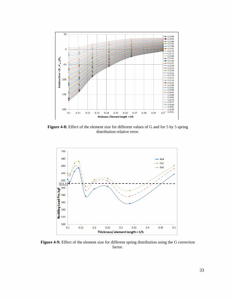
4.4.3 Effect of the element size
Figure 4-7 shows the trend of the buckling load values with respect to the element
thickness ratio. As the elements gets smaller the buckling load gets closer to the theoretical
value for a constant value of G. the convergence is at least of second order. The error plot in
Figure 4-8 shows that G has a significant effect on the error. For the same value of G
(0.0206), the error can be very large for size ratio of 0.1 however it’s very low for size ratio
of 0.2. However you can find another value of G for which the error is very low for size ratio
0.1 and very large for size ratio of 0.2. This behavior supports the previous behavior in
studying the effect of the number of springs on the results.
4.5 Discussion of the Numerical Results
It was found from the previous section that changing the shear stiffness of the springs
through factoring the material shear modulus has a significant effect on the numerical
buckling load. Using the linear correlation between the relative error and the shear modulus
G we can linearly interpolate the G at which there is a zero or near zero error. This could be
done in this problem because we know the theoretical solution. This is not the case in real
application where we do not know the true solution to interpolate the G value. In order to
estimate the G or introduce a correction for the G, we looked back at the spring shear
stiffness and how it was calculated. The calculation was based on a pure shear force applied
on the interface between the two elements. The idea comes from the analogy of the axial
stiffness. When we apply a tension force on a bar, the force needed to pull the bar end one
Page 38
28
unit is EA/L. The same idea applicable when you have two objects slide against each other,
the force needed to move one object a single unit is GA/L. However this is estimation seems
to not function well in case of thin plates. Another estimation may be introduced which is to
calculate the shear stiffness based on the beam analogy. The force needed to move a fixed
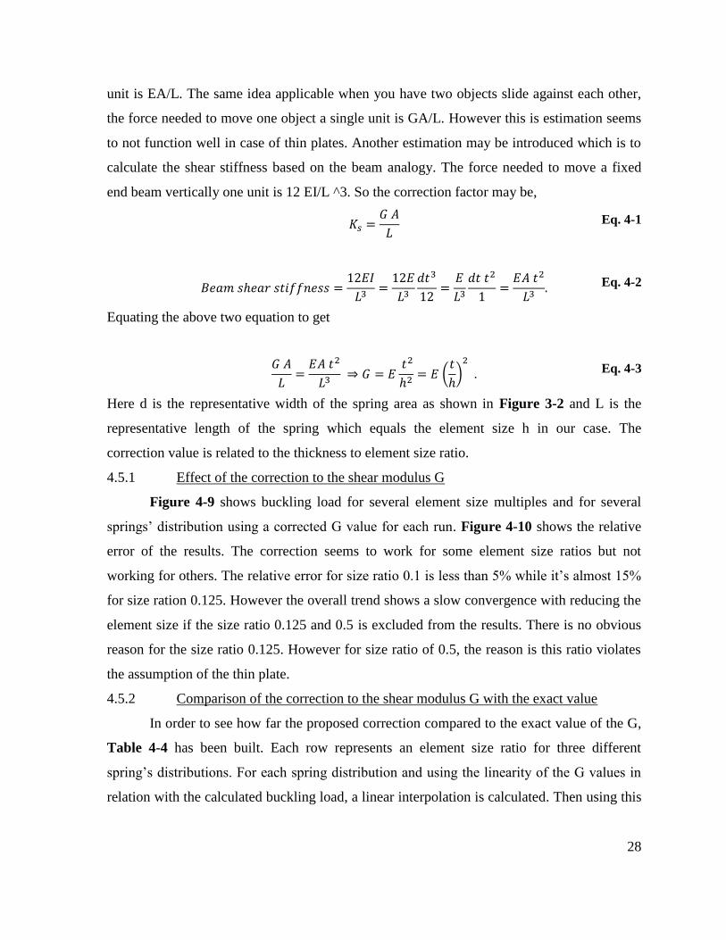
end beam vertically one unit is 12 EI/L ^3. So the correction factor may be,
Eq. 4-1
Eq. 4-2
Equating the above two equation to get
(
)
Eq. 4-3
Here d is the representative width of the spring area as shown in Figure 3-2 and L is the
representative length of the spring which equals the element size h in our case. The
correction value is related to the thickness to element size ratio.
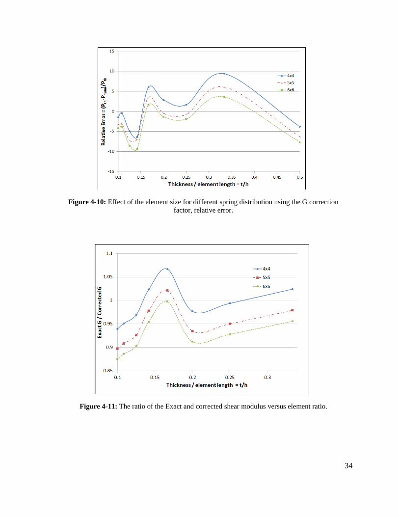
4.5.1 Effect of the correction to the shear modulus G
Figure 4-9 shows buckling load for several element size multiples and for several
springs’ distribution using a corrected G value for each run. Figure 4-10 shows the relative
error of the results. The correction seems to work for some element size ratios but not
working for others. The relative error for size ratio 0.1 is less than 5% while it’s almost 15%
for size ration 0.125. However the overall trend shows a slow convergence with reducing the
element size if the size ratio 0.125 and 0.5 is excluded from the results. There is no obvious
reason for the size ratio 0.125. However for size ratio of 0.5, the reason is this ratio violates
the assumption of the thin plate.
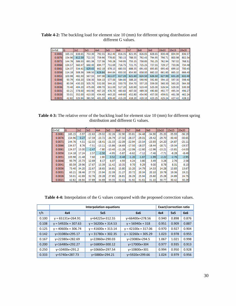
4.5.2 Comparison of the correction to the shear modulus G with the exact value
In order to see how far the proposed correction compared to the exact value of the G,
Table 4-4 has been built. Each row represents an element size ratio for three different
spring’s distributions. For each spring distribution and using the linearity of the G values in
relation with the calculated buckling load, a linear interpolation is calculated. Then using this
Page 39
29
interpolation a G value was calculated for a zero error and it’s called exact G. Then this value
has been used to obtain the buckling load to be sure that there is zero error when using the
exact G. Then the ratio of the exact G and the corrected G is calculated. Figure 4-11 shows
the relation between the ratio of the exact G and the corrected G for different element size
ratios. When the ratio is a unit it means that the corrected G is exactly the interpolated value.
In general the corrected G is within +/- 5% of the exact value.
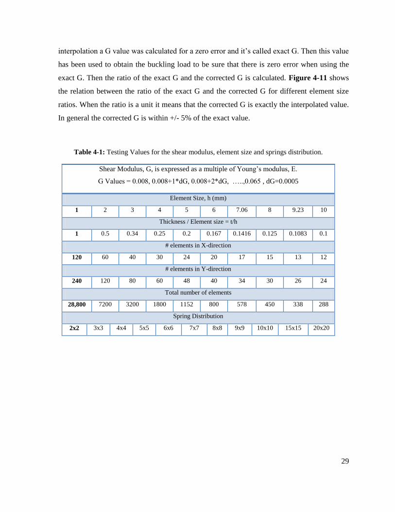
Table 4-1: Testing Values for the shear modulus, element size and springs distribution.
Shear Modulus, G, is expressed as a multiple of Young’s modulus, E.
G Values = 0.008, 0.008+1*dG, 0.008+2*dG, …..,0.065 , dG=0.0005
Element Size, h (mm)
1 2 3 4 5 6 7.06 8 9.23 10
Thickness / Element size = t/h
1 0.5 0.34 0.25 0.2 0.167 0.1416 0.125 0.1083 0.1
# elements in X-direction
120 60 40 30 24 20 17 15 13 12
# elements in Y-direction
240 120 80 60 48 40 34 30 26 24
Total number of elements
28,800 7200 3200 1800 1152 800 578 450 338 288
Spring Distribution
2x2 3x3 4x4 5x5 6x6 7x7 8x8 9x9 10x10 15x15 20x20
Page 40
30
Table 4-2: The buckling load for element size 10 (mm) for different spring distribution and
different G values.
Table 4-3: The relative error of the buckling load for element size 10 (mm) for different spring
distribution and different G values.
Table 4-4: Interpolation of the G values compared with the proposed correction values.
Interpolation equations Exact/correction ratio
t/h 4x4 5x5 6x6 4x4 5x5 6x6
0.100 y = 65131x+264.91 y=64225x+312.55 y=66400x+278.56 0.940 0.898 0.876
0.108 y = 54920x + 307.63 y = 56200x + 314.53 y = 56940x + 318 0.951 0.909 0.887
0.125 y = 40600x + 306.74 y = 41600x + 313.14 y = 42100x + 317.06 0.970 0.927 0.904
0.142 y=31080x+295.17 y = 31780x + 302.35 y = 32260x + 305.29 1.023 0.978 0.955
0.167 y=22380x+282.69 y=22860x+290.03 y=23080x+294.5 1.067 1.021 0.998
0.200 y=16480x+292.27 y=16800x+300.12 y=17000x+304 0.977 0.935 0.913
0.250 y=10400x+291.2 y=10660x+297.54 y=10800x+301 0.994 0.950 0.928
0.333 y=5740x+287.73 y=5880x+294.21 y=5920x+299.66 1.024 0.979 0.956
Page 41
31
Figure 4-4: Effect of number of springs for different values of G and for element size 10 mm.
Figure 4-5: Effect of number of springs for different values of G and for element size 10 mm
as a relative error.
Page 42
32
Figure 4-6: effect of the shear modulus (G) for different values of spring distribution and for
element size 10 mm.
Figure 4-7: Effect of the element size for different values of G and for 5 by 5 spring
distribution.
Page 43
33
Figure 4-8: Effect of the element size for different values of G and for 5 by 5 spring
distribution relative error.
Figure 4-9: Effect of the element size for different spring distribution using the G correction
factor.
Page 44
34
Figure 4-10: Effect of the element size for different spring distribution using the G correction
factor, relative error.
Figure 4-11: The ratio of the Exact and corrected shear modulus versus element ratio.
Page 45
35
CHAPTER 5
CONCLUSIONS AND FUTURE WORK
5.1 Conclusions
The effect of three parameters on the accuracy of the Applied Element Method in
obtaining the buckling load of a simply supported rectangular plate has been studied. The
three parameters are: the element size, the spring distribution and the shear stiffness of the
spring. In general the buckling mode produced by the AEM matches the theoretical solution
for a rectangular plate of aspect ratio of 1:2. There was a double half sine wave in one
direction and a single half sine wave in the other direction. Also the load- lateral deflection of
the plate is in a good agreement with what traditionally known about the buckling of plates
compared with the buckling of columns. The fundamental path bifurcates to a secondary
stable path upon reaching the buckling load.
It was observed that reducing the element size or increasing the number of the
spring’s distribution reduces the error in obtaining the buckling load. The rate of the error
reduction is at least of a second order. It’s worth mentioning that increasing the number of
the spring’s distribution from 10 by 10 to 20 by 20 has a little effect on the results. However
increasing the number of the spring’s distribution from 2 by 2 to 5 by 5 has improved the
results very much.
The shear stiffness of the spring has a big influence on the calculated buckling load. It
was found that the error is linearly depending on the shear stiffness. It was observed that a
zero error in the results can be obtained by linearly interpolating the value of the shear
stiffness. Since the shear stiffness is calculated as GA/L inside the software, and A and L are
properties of the spring dimensions then introducing a correction factor to the shear modulus
gave good results. The correction factor is based on the shear stiffness of a fixed-fixed beam
element.
Page 46
36
5.2 Future Work
The shear stiffness of the spring has a significant effect on the accuracy of the AEM
when modeling thin-walled structures like a thin plate. The correction factor introduced in
the study is not very accurate in all cases. Further studies need to be done to obtain
estimation for the shear stiffness. Also the accuracy of the AEM when modeling built-up
domains of several single plates to form an I or a C section need to be done.
Page 47
37
REFERENCES
ASI. Extreme Loading for Structures Theoretical Manual. Raleigh, NC: Applied Science
International, LLc., 2010.
Azevedo, N. Monteiro, and J.V. Lemos. "Hybrid discrete element/finite element method for
fracture analysis." Computer methods in applied mechanics and engineering,
2006: 195, 4579-4593.
Bazant, Zdenek P. Stability of Structures. New York: Oxford University Press, 1991.
Gambhir, Murari L. Stability Anaylysis and Desgin of Structures. Berline: Springer-Verlag,
2004.
Hun, A T. The Book of Irrelevant Citations. Ruston: Psychodelic Publishing Company, 2010.
J.M., Timoshenko, and Gere. Theory of Elastic Stability. New York: McGraw Hill Book
Company, 1961.
Jones, S A. "Equation Editor Shortcut Commands." Louisiana Tech Unversity, 2010:
http://www2.latech.edu/~sajones/REU/Learning%20Exercises/Equation%20Edito
r%20Shortcut%20Commands.doc.
Jones, S A, and K Krishnamurthy. "Reduction of Coherent Scattering Noise with Multiple
Receiver Doppler." Ultrasound in Medicine and Biology 28 (2002): 647-653.
Jones, S A, H Leclerc, G P Chatzimavroudis, Y H Kim, N A Scott, and A P Yoganathan.
"The influence of acoustic impedance mismatch on post-stenotic pulsed-Doppler
ultrasound measurements in a coronary artery model." Ultrasound in Medicine
and Biology 22 (1996): 623-634.
Kawai. "Recent developments of the Rigid Body and Spring Model (RBSM) in structural
analysis." Seiken Seminar Text Book, Institute of Industrial Science, The
University of Tokyo, 1986: 226-237.
Kawai, Tadahiko. "New Element Models in Discrete Structural Analysis." institute of
industrial science, university of Tokyo, 1977.
Kikuchi, A., T. Kawai, and N. Suzuki. "The rigid bodies spring models and their applications
to three dimensional crack problems." Computers & Structures, 1992: Vol. 44,
No. 1/2, pp. 469-480.
Lopez, J M, M G. Watson, and J M Fontana. "Writing Dissertations in New Word Formats."
LaTech Ph.D. Program (COES) 1, no. 1 (07 2010): 1-22.
Page 48
38
Love, A. E. H. "On the small free vibrations and deformations of elastic shells."
Philosophical trans. of the Royal Society (London), 1888: Vol. série A, N° 17 p.
491–549.
Meguro, Kimiro, and Hatem Tagel-Din. "Applied Element Simulation of RC Structures under
Cyclic Loading." ASCE, Vol 127, Issue 11, 2001: 1295-1305.
Mergheim, J., and E. Kuhl and P. Steinmann. "A hybrid discontinuous Galerkin/interface
method for te computational modeling of failure." Communications in numerical
methods in engineering, 2004: 20:511-519 (DOI: 10.1002/cnm.689).
Michaelstein, J. "Equation Editor." Microsoft Word 2010, The official blog of the Microsoft
OfficeWord Product Team, 2006:
http://blogs.msdn.com/b/microsoft_office_word/archive/2006/10/20/equation-
numbering.aspx.
Mindlin, R. D. "Influence of rotator inertia and shear on flexural motions of isotropic, elastic
plates." Journal of Applied Mechanics (Journal of Applied Mechanics, 1951, Vol. 18
p. 31–38), 1951: Vol. 18 p. 31–38.
N. Kawashime, M. Kashihara, and M. Sugimoto. "A combination of the finite element
method and the rigid-body spring model for plane problems." Finite Elements in
Analysis and Design, Elsevier, 1992: 67-76.
Pasluosta, Cristian Feder. Getting My Ph.D. Done! 1. Vol. 1. 1 vols. Ruston, LA: Argentina
Publications, 2010.
Przemieniecki, J. S. Theory of Matrix Sructural Analysis. New York: McGraw-Hill, 1968.
Reddy, and J. N. Theory and analysis of elastic plates and shells. CRC Press, 2007.
Reissner, E., and M. Stein. "Torsion and transverse bending of cantilever plates. ." Technical
Note 2369, National Advisory Committee for Aeronautics,Washington, 1951.
Xiong, Zhang, and Qian Lingx. "Rigid Finite Element and Limit Analysis." ACTA
Mechanica Sinica, 1993: Vol.9, No. 2, ISSN 0567-7718,.
Yoo, Chai H, and Sung Lee. Stability of Structures: Principles and Applications. Oxford, UK
: Elsevier Inc, 2011.
Yu, Wei-wen. Cold-formed steel design 3rd edition. New York: John Wiley, 2000.