20
Major, Klára – Drucker, Luca Flóra December 7, 2015 Macroeconomic impact of electric power outage – simulation results from a CGE modelling experiment for Hungary RESEARCH INSTITUTE
1
Major, Klára – Drucker, Luca Flóra
December 7, 2015
Macroeconomic impact of electric power outage – simulation results from a CGE modelling experiment for Hungary
R E S E A R C H I N S T I T U T E

32
R E S E A R C H I N S T I T U T E
MACROECONOMIC IMPACT OF ELECTRIC POWER OUTAGE
– SIMULATION RESULTS FROM A CGE MODELLING EXPERIMENT FOR HUNGARY
HÉTFA Research Institute and Center for Economic and Social Analysis
HÉTFA Working Paper No. 2015/12
Budapest
ISSN 2062-378X
Publisher: Major, Klára
Series Editor
HÉTFA Research Institute
H-1051 Budapest, Október 6. utca 19. IV/2.
Phone: +36 30/730 6668; Fax: +36 1 /700 2257
E-mail: [email protected]
www.hetfa.eu
HÉTFA Working Paper Series has been sponsored by the Pallas Athéné Domus Animae Foundation.
Graphic design: Kriszta Parádi
ABS TRACTThis paper presents the results of a CGE application that is used to measure and understand how secto-
ral shocks might influence the Hungarian economy, its economic agents and its different industries. The
electricity outages are modelled by the decrease in the supply of energy. The capital stock in the energy
industry is shocked, which leads to a decrease in the supply of energy. It is assumed that energy is a close
complement to other goods both in production and consumption. In the base scenario a 2.08% decline in
the supply of energy leads to a 0.53% decline in the GDP. Without price rigidities and other frictions, the
adjustment is mainly driven by agents who can react at the lowest price. Therefore, this estimation should
be considered as a lower bound on the real costs of adjustment. It is also shown that if prices are distorted,
the costs of an outage is higher.

54
Asymmetric or sectorial shocks actually occur regularly in modern economies. Their impact on the ove-
rall economy seems a more important issue today as economies are more globalized, and inter-sectorial
(input-output) linkages lead to spillover effects in the economy. Even though it might be important from
a historical point of view to understand how large those spillover effects are today in comparison to
their values in the past, now we aim to come up with answers for a smaller subject: we argue that CGE
models are adequate tools for measuring the size of those impacts. In this paper a CGE model application
is introduced to measure the impact of a sectorial shock on the Hungarian economy.
Our work is partly motivated by a recent example of an electricity outage in Hungary. Due to the heavy
storm on 17 August 2015 in Hungary, thousands of households were without electricity for days, because
rain flooded the cellars of houses, where transformers were placed.1 According to the Budapest Business
Journal2, 9000 homes suffered from outage for a longer time, while in 47000 homes there were temporary
blackouts. The Hungarian electricity supplier, ELMÛ paid a compensation of 5000 HUF (around 16 EUR) to
the households, where electricity supply was stopped for more than 24 hours.3 The total damages caused
by the storm are estimated to amount to 1.6 billion HUF (see MABISZ 2015).
This example motivated our work to a large extent as energy is one of the crucial inputs of production
(and also an important product in consumption). Nonetheless, there is an even more recent example of
a potentially dangerous sectorial shock. By the time of the writing of this paper, in September 2015 the
Environmental Protection Agency (EPA) has found that some models with diesel engines produced by the
German Volkswagen company emit much more harmful gases than allowed. The cars emitted around 40
times more nitrogen oxides than allowed in the USA. These cars could pass the tests because the built-in
software could detect if the car was tested at the moment and artificially reduce the performance. Thus,
the emission of harmful gases did not reach the allowed maximum amount. The company admitted that
around 11 million cars were concerned worldwide.4
The authors want to thank Pálma Szolnoki for her ideas and help in understanding the details how the energy market works in Hungary. However, any mistakes and errors are the authors’ responsibility.
1 http://index.hu/belfold/budapest/2015/08/19/aramszunet/2 http://bbj.hu/budapest/storm-floods-the-streets-of-budapest_102670 3 http://www.penzcentrum.hu/otthon/5_ezer_forintot_kaphatnak_az_elmu_ugyfelei_az_aramszunet_miatt.1046052.html4 http://www.bbc.com/news/business-34324772
INTRODUCT ION
5 http://www.theverge.com/2015/10/16/9552611/volkswagen-europe-recall-announced6 http://www.origo.hu/gazdasag/20151012-vw-botrany-hatasa-magyarorszag-londoni-elemzok.html7 http://hvg.hu/gazdasag/20151008_Sokkal_tobb_manipulalt_motor_keszult_Gyor8 http://www.origo.hu/gazdasag/20151012-vw-botrany-hatasa-magyarorszag-londoni-elemzok.html
The scandal causes extreme costs to the company, since it announced to recall all vehicles in Euro-
pe and in the US with the diesel engines concerned “at no cost to our customers”5 and fix the engines.
Furthermore, the EPA is able to fine the company for each car in the USA that broke the regulations up
to $37500, which in total would cost around $18 billion to the company. Not to mention the decline in
share prices, costs of loss in reputation and the trust of customers in Volkswagen and in diesel engines
themselves.
This is an important example as the expected decline in the production of the Volkswagen company
would affect several Central-Eastern European countries, including Hungary.
According to an article referring to a Barclays report,6 4% of the world’s production of vehicles is located
in Central and Eastern Europe, which means around 1.5 million jobs. Volkswagen Group owns 12 vehicle
brands, including Audi that operates a plant in Hungary, where 3 million of the manipulated engines were
produced.7 Volkswagen Group has 43 percent share in the car production of the CEE-region; therefore, a loss
in the production of the company would affect the production in these countries severely. In the Barclays
report they modelled a 20 percent decline in Volkswagen’s production. The results of their simulations
show that this would cause a 0.02-0.58 percent decline in GDP in Hungary with a direct loss of 0.24 percent
of GDP. However, the total costs from further negative effects – reducing work-time, layoffs, decline in
retail trade – could be twice or three times larger. The study of the Bank of America Merrill Lynch reports
that in a worst case scenario the Hungarian GDP growth could decline by 1-1.5 percentage points.8
In this paper we provide a CGE approach to measure the economic impacts of a sectorial shock, namely
an electric power outage. The structure of the paper is as follows. In Section 1 a short summary is given
on the existing approaches estimating the loss caused by an electricity outage. In Section 2 characteristics
of electric power outages are described. Section 3 describes the energy producing sector of Hungary and a
specification in more details of the estimation question. In Section 4 the main building blocks of the applied
CGE model is described. In Section 5 the data background and the calibration work is shown. Also, the
different scenarios are introduced here. In Section 6 the results of the simulations are presented. The final
chapter concludes the paper.

76
1. APPROACHES OF ES T IMAT ING THE LOSS C AUSED BY AN E LECTR IC I T Y OUTAGE
The costs of power outages are measured by different techniques. Reichl et al. (2013) analyse the existing
assessment methods quantifying socio-economic effects of the outages. They introduce these measures on the
example of Europe and emphasise that continuous electricity supply is essential for an economy; therefore, security
measures must be made to provide uninterrupted supply.
They argue that there is an increasing need for securing continuous power supply, because electricity production
and distribution is changing now in Europe: electricity markets are undergoing liberalization in EU member countries;
and therefore, new regulations are needed for ensuring supply security. Second, inputs from renewable energy
sources are growing, and these energy sources cannot be used continuously. Third, electricity consumption grows
steadily as well; therefore, supply security is very important.
To create an efficient regulatory system for supply security, its value must be assessed. This value is often
associated with the loss caused by the shortage of supply security. To model the economic loss caused by power
outages, they distinguish three categories of effects of the electricity outages: direct costs, indirect costs and resulting
long-term costs of macroeconomic relevance. Direct costs occur immediately after a natural disaster or technical
problem causing the outage, while indirect costs are the results of direct effects, e.g. decline in production caused
by the absence of electricity supply. Examples for long-term economic effects may be rising prices for production
equipment because of the increased need for backup systems; or the availability of continuous electricity supply,
which can be a major factor for a firm in choosing business location.
Several studies examined the effects of outages in the CGE framework. Rose et al. (2007) have investigated the
impacts of an electricity outage caused by a terrorist attack on parts of the electricity supply system. They cite that
costs of damages caused by outages are often measured only by the costs of precautionary actions made in order
to avoid the outages. However, their paper gives attention to resilience of the economy on corporate, industrial or
regional level, as well as indirect economic effects such as multiplying effects and general equilibrium effects; and
they emphasise that these also need to be taken into account when estimating the costs of damages.
An electricity outage first of all has immediate, partial equilibrium effects, such as costs incurring from the
damage caused in the equipment. These costs can be interpreted as loss in profits. In addition, there are other
direct effects such as costs of backup-systems, rescheduling of production and increasing the capacities of the utility
system. They measure the marginal value of the costs of electricity outage by the marginal reliability on electricity –
the more capable the system is of adapting to the new circumstances, the less reliable it is on electricity; therefore,
the smaller the loss is caused by the outage.
However, outages also have indirect or general equilibrium effects. The authors measure general equilibrium
effects via economic output loss through different channels: loss of the downstream consumer of a firm that
suffered damages. Upstream suppliers of the damaged firm suffer from economic loss, as well, since the firm
ceases to order input from them. The wages decreased in firms that suffered directly from the damage; therefore,
other firms have to face losses of consumer demand because of lower wages. Investment also decreases because
of the profit decrease of disrupted firms, and this results in reduced output, as well. Similarly, the increased costs
of firms with damaged equipment reduce output and productivity. CGE models in general are adequate tools for
measuring these indirect effects.
Xie et al. (2014) also investigate the effects of economic disasters in a CGE framework, with special regard to
the positive effects of reconstruction after a disaster. They model the direct, immediate effects of the disaster with
decreasing capital stock; however, reconstruction works reproduce this capital stock in the following years. The
article introduces the model on the example of the 2008 Wenchuan earthquake, by comparing three scenarios: no
disaster, disaster and reconstruction, and disaster but no reconstruction. They also emphasise the importance of
economic resilience: they distinguish static and dynamic resilience. Static resilience means the ability to continue
production after a shock caused by a disaster, while dynamic one means the speed by which the economy recovers
after a shock.
A natural disaster affects the economy through more channels: if a production plant is damaged, production
declines or stops; raw materials and the number of workers decrease. Capital stock also decreases; therefore,
aggregate supply decreases. It affects the whole production chain, causes unemployment and thus lowers income,
and because of low production tax income decreases, too. The disaster affects not only the sector where it caused
damage, but also has external effects on other sectors. However, reconstruction after the disaster has positive supply
and demand effects. On the supply side, reconstruction investments restore capital stock in the following periods;
therefore, aggregate supply gradually increases. On the demand side, because of the need for reconstruction,
investment demand grows, especially in areas damaged by the disaster. The government and the households also
increase their demand for goods needed for reconstruction; therefore, aggregate demand increases, too.
The authors find that without reconstruction works every sector suffers from economic loss, ; however,
with reconstruction investment demand increases immediately. Therefore, the output of the construction
sector and building material industries grows in the first years following the disaster. Employment instantly
decreases; however, with reconstruction works it grows gradually in the next years. Nevertheless,

98
9 http://nation.time.com/2012/11/26/hurricane-sandy-one-month-later/
unemployment is still higher than in the scenario without natural disaster. Employment shifts from other
sectors to the construction sector and building material industries because of the increased demand for
workers in these sectors. The income of the residents decreases immediately, and remains lower than in
the scenario without disaster in the next years. However, it increases gradually due to reconstruction, so
the differences decrease.
Küster et al. (2007) investigate energy policy measures in a CGE framework, with special regard to
their impact on labour market. Labour market imperfections are introduced to the model via wage curves
and constraints on minimum wages. They analyse the effects of capital subsidies on the application
of technologies that use renewable energy sources. Their findings indicate that these subsidies do not
necessarily result in decreasing emission. Furthermore, they may have negative growth effects if they
promote renewable energy sources that are not cost effective, thus increasing unemployment in skilled
and unskilled labour, as well.
These examples show that CGE models with their rich details about the sectorial structure of the
economy provide adequate tools for understanding how the indirect effects of a sectorial shock spill over in
the economies influencing (or, potentially harming) other industries. Their general equilibrium modelling
framework makes it possible to understand how large those indirect effects are, and the estimation of the
losses and damages that a disaster causes may go beyond the listing of the direct (recovery) costs.
2 . CHARACTER IS T I CS OF E LECTR IC POWER OUTAGES
As CGE models are very abstract tools to estimate real life events, it is important to understand what
the main important questions are when a certain event is modelled. Definitely, in the case of electricity
outages, the damages are strongly related to technical specifics: electronic appliances do not work without
electricity. These technological connections pervade everyday life and are present basically at every activity.
In order to find the most relevant mapping of an electricity outage to the language of the CGE models, we
scrolled over some recent and very influential examples of such events.
For example, in the USA electricity outages due to natural disasters are not rare. Hurricane Sandy
in October 2012, for instance, caused power outages in 17 states with around 8 million homes losing
electricity, many of them for more days.9 That is why in 2013 a study was conducted by the U.S. Department
of Energy’s Office of Electricity Delivery and Energy Reliability (see Executive Office of the President (2013))
on the economic costs of these outages and the possible benefits of increasing the resilience of the electric
grid to outages caused by severe weather.
One of the largest nuclear accidents, the disaster of the Fukushima Daiichi Nuclear Power Plant and
the earthquake preceding it on 11 March 2011 caused a major shortage of electricity in Japan. Due to
the earthquake and tsunami Tokyo Electric Power Company (TEPCO) and Tohuku Electric Power Company
(Tohuku EPCO) lost 22% and 45% of their capacity, respectively. The service areas of the two companies
suffered from losing electric power; this affected about 8.5 million households. Because of the damaged
power plants rolling blackouts had to be initiated for 3 hours per day for two weeks after the earthquake
in some areas.
However, these planned blackouts were not in every area and next day’s rolling blackout was announced
the day before, which caused confusion. Therefore, the government called upon people to reduce their
consumption of electricity to avoid further rolling blackouts. The target was a 15% cut in peak consumption
of energy in the areas of TEPCO and Tohuku EPCO. Business facilities also had to conserve electricity by e.g.
adjusting business hours or saving on air conditioning. For large firms with more than 500kW of demand
the 15% conservation between July and September was obligatory. Electricity utility companies had to post

1110
10 http://www.balkaninsight.com/en/article/albania-doing-little-to-quell-growing-demand-for-electricity11 http://albaniaenergy.org/acerc%20english-2/Project%20Platform/Articles/Reforms%20on%20Electricity%20
Sector%20in%20Albania.html
forecasts of daily electricity using and reserve capacity ratio on their websites. The Ministry of Economy,
Trade and Industry gave coupons to people who could save the target amount of energy.
The campaign was successful: electricity conservation ratios – the amount of electricity consumption
spared compared to last year’s consumption – of households were 7.4% for whole Japan and 11.7% and
8.9% in TEPCO’s and Tohuku EPCO’s service areas right after the disaster. The total savings in summer
consumption of 2011 compared to 2010 were 19% in Tokyo and 18% in Tohuku areas. Large firms (with
a higher than 500 kW contract demand) saved 27% and 18% in the two areas, respectively. Small firms
saved 19% and 17%, while households conserved 11% and 18%, as well. In the third area, Kansai, where
energy conservation was voluntary, there was still an 8% reduction (see Murakoshi et al. 2012 and Kimura
and Nishio 2013). This is an interesting example revealing that differences in adjustments of actors might
be an important issue.
Large electricity outages do not only happen overseas. A major electric power outage occurred in Europe
on 4 November 2006, when the Ems Overhead Powerline Crossing in Germany was disconnected to allow a
ship to pass under the cables. Although this was a planned and prepared event, it caused an interruption of
the East-West power flows of international power trade. The Western area suffered from a frequency drop and
electric power supply was stopped for about 15 million households in Europe (see UCTE Final Report 2007).
These important examples show that electricity outages in most developed countries are usually one-
time events – even if they are expected or unexpected. However, there are examples of regular electricity
outages, too. In Albania around 98% of the electricity production comes from hydropower, with the most
important plant being on the River Drin (see EBRD 2008). Therefore, production highly depends on weather
conditions. Before 2008 the yearly amount of energy produced varied between 3000 and 6000 GWh. Since
electricity consumption is growing in Albania, and due to changes in the amount produced, electricity im-
port varied strongly, as well. In very dry years insufficient production could lead to electricity shortages, e.g.
in 2007 a drought caused major electricity outages of 16 hours a day in some areas (Ebinger 2010). In 2006
electric power shortages cost 1% of GDP growth in Albania, while according to estimations total protection
from electricity outages would have cost 1.6 billion dollars.10 Energy security is thus a very important issue
in Albania, and actions were taken to adapt energy production to the variable weather and changing
climate. In 2008 the Albanian government signed a contract to build a new hydropower plant that started
to operate in 2013 (see IFC 2013). In 2014 reforms of the electricity sector were started to increase supply
reliability.11
As these examples show in most situations electric power outages unexpectedly lead to a discontinuation
of the otherwise ongoing economic activities. These sudden and usually not foreseen changes in the supply
(or availability) of electricity influence households’ behaviour, as many different activities from household
work to recreational activities require energy. Production process might also be interrupted in an unexpected
way resulting in loss of inputs (producing waste product), losing work-time and lower supply of product.
Even if a list with all the different aspects of an outage were long, one common feature of these aspects
is that they appear in almost every segment of the economy. The costs related to outages are far more
widespread in the whole economy than the direct costs of recovering the materialized productive capital of
the energy system. Therefore, understanding how large those indirect effects could be is a useful task.
It is also apparent that in most cases electricity outages occur unexpectedly and have serious impact
on everyday life for a shorter or longer horizon. However, when electricity outages are present for a longer
time period, sooner or later they will be expected. It is reasonable to assume that this latter case can be
described only if expectations are formed endogenously in the given estimation approach. In this latter
case, regular outages may be discouraging investment and will influence allocation decisions made in time.
In our application we aim to model the economic costs of an unexpected electricity outage that is present
for a shorter time horizon (up to a few months). We will not take into account how the longer presence of
shortage in electricity influences future plans and the dynamics of an economy. Therefore, the electricity
outage is modelled by the decrease in the supply of energy.
As it seems from the above examples, sometimes electricity outages are frequent (for a short period
of time, like in the Japan case) but each occasion lasts only for a few hours. This is dramatically different
from the scenario when electricity is not available for complete days or even weeks (like in the European
example). Unfortunately CGE models are not detailed enough to make reasonable difference between
these two scenarios. Nonetheless, they must be distinguished in the application as these require different
responses from the agents. A one-time large shock will result in the loss of inventories, producing waste
instead of valuable products and the complete loss of work-time. The substitutability of electricity in these
cases depends upon previously established solutions, like former adaptation of uninterruptible power
supply systems, to a great extent. However, as an opposite “scenario”, when electric outage is present for
a few months but only up to a few hours each day, the damages are different and adjustment to the shock
could happen with re-organising economic activities.
As CGE models are best used to understand the indirect, economic impacts of sectorial shocks of moderate
size, it is more reasonable to assume that there are regular bottleneck capacities in the economy, which
lead to regular but not very long-lasting electricity outages. As an approximation let us assume that
due to some unexpected event (like a natural disaster) shortage of electricity occurs, which needs time
to fully recover. Therefore, electricity is not available for two hours every day for three months (outside
heating season). This is basically a 1/48 size decrease in the supply of electricity. Therefore, we build our
application to measure the economic costs of a 1/48 decrease in the supply of electricity.
1312
3 . ENERGY SECT OR IN HUNGARY
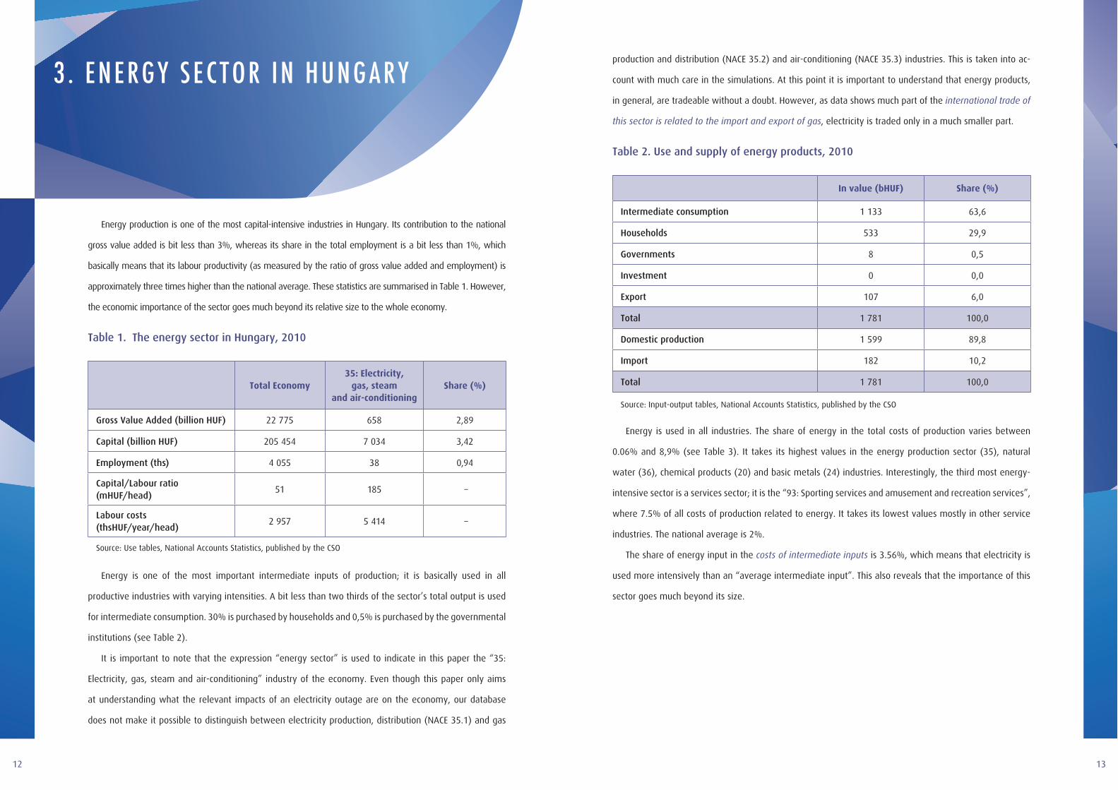
Energy production is one of the most capital-intensive industries in Hungary. Its contribution to the national
gross value added is bit less than 3%, whereas its share in the total employment is a bit less than 1%, which
basically means that its labour productivity (as measured by the ratio of gross value added and employment) is
approximately three times higher than the national average. These statistics are summarised in Table 1. However,
the economic importance of the sector goes much beyond its relative size to the whole economy.
Table 1. The energy sector in Hungary, 2010
Total Economy35: Electricity,
gas, steam and air-conditioning
Share (%)
Gross Value Added (billion HUF) 22 775 658 2,89
Capital (billion HUF) 205 454 7 034 3,42
Employment (ths) 4 055 38 0,94
Capital/Labour ratio (mHUF/head)
51 185 –
Labour costs (thsHUF/year/head)
2 957 5 414 –
Source: Use tables, National Accounts Statistics, published by the CSO
Energy is one of the most important intermediate inputs of production; it is basically used in all
productive industries with varying intensities. A bit less than two thirds of the sector’s total output is used
for intermediate consumption. 30% is purchased by households and 0,5% is purchased by the governmental
institutions (see Table 2).
It is important to note that the expression “energy sector” is used to indicate in this paper the “35:
Electricity, gas, steam and air-conditioning” industry of the economy. Even though this paper only aims
at understanding what the relevant impacts of an electricity outage are on the economy, our database
does not make it possible to distinguish between electricity production, distribution (NACE 35.1) and gas
production and distribution (NACE 35.2) and air-conditioning (NACE 35.3) industries. This is taken into ac-
count with much care in the simulations. At this point it is important to understand that energy products,
in general, are tradeable without a doubt. However, as data shows much part of the international trade of
this sector is related to the import and export of gas, electricity is traded only in a much smaller part.
Table 2. Use and supply of energy products, 2010
In value (bHUF) Share (%)
Intermediate consumption 1 133 63,6
Households 533 29,9
Governments 8 0,5
Investment 0 0,0
Export 107 6,0
Total 1 781 100,0
Domestic production 1 599 89,8
Import 182 10,2
Total 1 781 100,0
Source: Input-output tables, National Accounts Statistics, published by the CSO
Energy is used in all industries. The share of energy in the total costs of production varies between
0.06% and 8,9% (see Table 3). It takes its highest values in the energy production sector (35), natural
water (36), chemical products (20) and basic metals (24) industries. Interestingly, the third most energy-
intensive sector is a services sector; it is the “93: Sporting services and amusement and recreation services”,
where 7.5% of all costs of production related to energy. It takes its lowest values mostly in other service
industries. The national average is 2%.
The share of energy input in the costs of intermediate inputs is 3.56%, which means that electricity is
used more intensively than an “average intermediate input”. This also reveals that the importance of this
sector goes much beyond its size.

1514
4 . MODEL DESCR IPT ION
We apply a dynamic CGE model for estimating the impact of an electricity outage. The core of the model is
a standard, static CGE model which has been modified for the purpose of this analysis in the following aspects:
1. Firms utilize two primary factors in production, namely labour and capital. However, unlike in a
standard CGE model, in our application capital is not mobile across sectors. Capital is given by past
investment and depreciation in each sector, only labour input is free to adjust to the shocks.
2. Labour market is modelled following efficiency wage theories, which make it possible to simulate
the impact on (involuntary) unemployment, as well.
3. Recursive dynamics has been added to follow how investment decisions influence the path of capital.
Finally, the energy sector is modelled differently from the rest of the economy, as the counterfactual
scenarios are drawn by adding exogenous shocks to the energy supply system (through a decrease in the
productive capital stock of this sector). We describe briefly each block of the model below.
4.1. THE STATIC MODEL The core of the CGE model is a set of static equations describing the behaviour of the agents, their decisions
about consuming, producing goods and services. As a result of their decision, the flows are completely
determined and influence the time path of the stock variables as it is shown in the section on dynamics.
4.1.1. HOUSEHOLD BEHAVIOUR
The representative household shares its income between savings and consumption. The primary income
of the household equals the income generated in production, since the household is the only owner of
factors of production. It pays tax on the income of primary factors of production, and furthermore, it
receives a transfer from the government. In the static CGE framework savings are exogenous; however, in
our application the savings rate is driven by the past real interest rate. Disposable income of the household
is therefore given as the difference of primary income and savings, transfers and taxes.
Table 3. Sectoral average shares of energy costs in production
Total Costs Materials' costs
minimum of shares 0,31 0,41
maximum of shares 8,85 18,88
simple average of sectoral shares 2,32 4,53
standard deviation of shares 2,06 3,93
Source: own calculation based on Input-output tables, National Accounts Statistics, published by the CSO
Nonetheless, the energy dependences of the industries are quite different. As our kernel estimation
shows (see Figure 1), there are a few industries with relatively higher energy intensity, but in most of the
sectors the share of energy in total costs of production varies between 0 and 4%.
Figure 1. Histogram and kernel density of sectoral average shares of energy costs in
production
0.1
.2.3
0 2 4 6 8
histogram density

1716
The household decision is described in a three-tier nested structure (see Figure 2). It maximises its
intratemporal utility by making choices on aggregate consumption and leisure. The utility level of aggregate
consumption is a CES aggregate of consumption of energy product and all other goods. Finally, the composition
of all goods is given by another CES aggregate. This makes it possible to parameterize the elasticity of
substitution between energy and other goods independently of the substitution between other goods.
Figure 2: Nesting structure of consumption goods and leisure
Utility
Free time(labor supply) Consumption
Energy All other goods
Single good Single good
4.1.2. PRODUCTION BLOCK
The relationships between factors of production and the goods produced follow the structure of the
standard CGE models. Therefore, the products of different sectors are used for intermediate inputs and for
final use, as well. The structure of the relationships is shown in Figure 3.
1. First, primary factors of production (capital and labour) are aggregated to a composite factor of
production using CES function. Thus, the elasticity of substitution between labour and capital can be
parameterized.
2. The domestic supply of goods using the composite factor and intermediate inputs for production. We
assume Leontief technology at this level. Therefore, both the composite factor and the intermediate
inputs are used in fix shares in the production of goods.
3. Domestic output is sold both at home and abroad. The usual transformation function is used to split
domestic production between domestic sale and export. The transformation function utilizes the price
differences between domestic sale and foreign sale, and it assumes final elasticity of substitution,
thus avoiding perfect specialization (thus reaching a “corner solution”) in the production of the goods.
4. The goods finally consumed are either produced domestically or imported. Goods for final use are
aggregated by Armington’s aggregation functions from domestic goods and import goods. This
method is similar to the transformation function approach: by introducing final price elasticities,
domestic and foreign goods are considered as not perfect substitute to each other.
5. The composition of domestic demand is the following: private consumption, government expenditure,
investment demand and intermediate inputs.
Technically, the production decision is modelled in a nested structure. Firms take the prices of inputs and
the prices of their products as given at every decision level. At the first level firms use primary factors of
production (labour and capital) to obtain the composite factor. The technology of production is described by
a CES production function. The demand of the different sectors for primary inputs can be derived from the
profit maximization of the firms. At the second level firms produce their goods from the composite factor of
production and intermediate inputs. At this level aggregation is modelled by Leontief technology, assuming
that the composite factor and the intermediate inputs are used at fixed ratios in production. The demand
function of factors and the supply function of products are derived from the profit maximization decisions.
Figure 3. Production and use of goods in the tradeable industries
Utility Household consumption
Import Domestic goods
Domestic production
Composite factor
CES or C-D production function
Leontief technology
Transformation (CES) function
Armington (CES) function
Equilibrium
Capital Labour
Intermediate inputs
Export
Armington’s goods
Government expenditure Investment demand Intermediate inputs
We assumed that the amount of capital is given by past decisions on investment and depreciation
(however, the whole process is completely exogenous). Therefore, there is no market for capital in the
model. The income share of the capital is modelled as gross operating profit and is given to the households,
it forms part of their primary income.
Foreign trade is modelled assuming that Hungary is a small, open economy. Therefore, by assumption

1918
the world price of export and import goods are exogenous and given in foreign currency. The real exchange
rate is applied to calculate the price of export and import goods in terms of domestic currency. The foreign
savings is also expressed in foreign currency.
Goods produced domestically and imported goods are not perfect substitutes; therefore, it is important
to define composite goods that express the relationship between domestic and imported goods. Therefore,
for tradable goods the so-called Armington aggregation functions are used, where a parameter shows the
substitutability of foreign and domestic goods. From these functions demand for domestic and imported
goods can be derived.
Domestic goods are either consumed in the country or are exported. These two types of use are
expressed by a transformation aggregation function where the elasticity of substitution is described by a
parameter. The domestic supply and the supply for exports can be derived from this function.
4.1.3. PRODUCTION IN THE ENERGY SECTOR
Production in the energy sector is modelled differently than the other sectors. We assume that in the
energy sector the technology is Leontief at every level of the nested structure for domestic production;
therefore, supply of energy requires primary inputs and intermediate inputs in given ratios. As capital is
fixed and not mobile across sectors, the supply of energy is completely determined by the available amount
of capital in the sector. The demand for other inputs, like labour and intermediate inputs adjust according
to the given technology parameters.
This specification makes it possible to shock the supply of energy in a very simple manner. As the available
capital in the energy sectors decreases, there is a similar decrease in the supply of energy. Our simulation
experiment aims at understanding how and to what size this shock is going to influence the rest of the economy.
4.1.4. GOVERNMENT
The incomes of the government are determined endogenously, while the expenditures are exogenous.
The income of the government comes from two parts: indirect taxes stemming from the use of products and
direct taxes levied on the primary factors of production. Expenditures of the government are governmental
consumption and transfers paid to households. The primary balance of the budget is the difference of the
incomes and expenditures that is expressed as a percentage of GDP, as well.
4.1.5. LABOUR MARKET
In standard CGE models labour market as well as the other markets clear due to the adjustment of the
real wage, and thus unemployment occurs only voluntarily. However, in the last decades several ways of
modelling labour market rigidities were implemented in CGE framework; for an excellent summary of
these methods see Boeters & Savard (2012). In the present model labour market rigidities are introduced
following efficiency wages theory.
In the efficiency wages model the equilibrium wage is determined as the intersection of the labour
demand curve and the wage curve. Since this wage level is not necessarily the one where labour supply
and demand are equal, there is an oversupply of labour in the market; thus, there is unemployment. The
wage curve is the result of an incentive situation stemming from the information asymmetry between
employers and employees. The firm wants to determine a wage by which workers are incentivized to
work hard; therefore, the utilities of workers from working must be at least the utility from shirking. The
parameterization of the labour market follows Boeters & Savard (2012).
4.1.6. MARKET EQUILIBRIUM
As the present model has a general equilibrium framework, equilibrium must hold in all markets;
therefore, total consumption of every tradable good must be equal to the sum of the supplies of the
import and domestic production. As for non-tradable goods, domestic supply must equal to domestic
demand. Trade balance and the balance of the capital account add up to determine savings of the rest
of the world. The investment-savings balance holds as domestic investment can only be financed from
domestic savings and foreign savings.
Equilibrium must hold in the market of production factors, as well. However, in the labour market
it means that the difference between labour demand (as is defined by the sum of sectorial labour
demand) and the labour supply (from household utility maximization problem) defines unemployment.
However, this unemployment rate must be consistent with the wage specified by the wage curve.
4.1.7. CLOSURE RULE
The macroeconomic aggregates of a static CGE model are not fully determined. As it is usual in
this modelling environment, a so-called “closure rule” is applied. Closure rule means to identify which
macroeconomic variable is considered as being exogenous in order to fully specify the macro level of
the model. In our application the investment-driven closure rule is applied. We assume that the model
simulations aim at measuring the impact of a short-run event without having any significant impact on
future plans, including investment. Therefore, (sectorial) investment demands are taken as exogenous.

2120
4.2. DYNAMICS The characteristics of the system described above determine the static equilibrium of the model.
However, for describing the time path of the economy dynamics should be added. Dynamics of a model
can either be forward-looking or backward-looking. In the present model recursive dynamic relationships
are used; therefore, past and present values determine the initial values of the next period.
These recursive relationships are the following: (1) capital stock increases with investments and
decreases due to depreciation. (2) Net foreign debt of the country is the debt of the previous period
increased by payable interests and decreased by redemption, which is expressed by the balance of trade
of the country. Real interest rates are determined by the foreign real interest rate. Risk premium related
to the debt of the country is a nonlinear function of the indebtedness of the country, and is modelled by
a so called linex function that punishes high indebtedness strongly. The savings rate of the household is
exogenous; however, it may change in time due to the changes in the real interest rate. In this model it is
assumed that the lagged value of the real interest rate affects the savings rate of the household.
5 . C ASE DESCR IPT ION AND DATA
5.1. DATA The parameterization of any CGE model requires enormous effort from the model builder. The core data
source of the parameterization is the published input-output tables that are estimated by the Central Statistical
Office of Hungary. These tables are published for every fifth year, the last available has been published for
2010. Thus, we based our estimation experiment on this table and collected other statistical information
of 2010 to finalize parameterization. In some cases missing information were utilized from other sources;
however, in each cases we aimed to avoid using data of different years.
The input-output data has been completed with data on income flows between different agents of the
economy by creating a consistent social accounting matrix (SAM). The SAM in our application follows the
standard structure (see Table 4). There are 62 different sectors of the economy that are distinguished in the
application. The energy sector is one of these, so there are 61 sectors that are influenced indirectly in our
application, and the energy sector is shocked directly.
The “upper right” and “bottom left” blocks of the SAM (as denoted by different shading) are also part of
the published input-output tables; however, we needed to make small data corrections (these are described
in detail below). The “bottom right” block of the SAM contains some non-market income flows (transfers
and taxes) between the different agents that are not part of the input-output tables, so these cells have
been filled with additional information from the national account statistics that are published by the CSO.
From these statistics we utilized information on how much tax has been paid by the households, these were
interpreted as taxes on labour. The taxes paid by the firms were interpreted as taxes on gross operating pro-
fit. The transfers from government to households have been added to the model. By the addition of these
statistics we could model the change in the primary budget balance of the government and the overall sum
of private savings, which now has been assigned to the household sector.

2322
Table 4. Social Accounting Matrix
Sectors Factors Taxes Final consumption
CAP LAB DTX IDT HOH GOV S-I RoW
Sectors
CAP
LAB
DTX
IDT
HOH
GOV
S-I
RoW
!!,!
!"#! w∙ !!
!!,!
!"# w∙ !
!! !!
!!
!!
!"! !"! !"! !!
! ∙ !! !!
!"
!!
The accounts of the SAM are indicated as follows: CAP = capital, LAB = labour, DTX = direct taxes, IDT = indirect taxes, HOH = households, GOV = government, S-I = savings-investment balance, RoW = rest of the world. Income flows are indicated in the cells of the tables. Any cell without a variable in it indicates zero income flows. The notations are the following: X: intermediate and final consumption, GOP = gross operating profit, w: real wage, L: employment, Tz: indirect taxes, Td: direct taxes, M: import, E: export, S: savings, ε: real exchange rate. Sectors are indicated by i and j.
The published data needed some small corrections as it had to fit to the model requirements. We made
three important changes to the data. First, we had to eliminate re-export from the sectoral international
trade data. The symmetric input-output tables for import (published by CSO) contain information on how
large part of the import is used directly for export. These data have been extracted from the original ex-
port and import values for each sector. This modification had no implication on the sum of the net export.
At the same time it is rather crucial from our application’s point of view. As it turned out, there are three
sectors of the economy with extraordinary degree of openness. In the “26: Computer, electronic and optical
products”, “27: Electrical equipment” and the “29: Motor vehicles, trailers and semi-trailers” sectors the
value of export is higher than the value of domestic production. Similarly, the value of import exceeds the
value of domestic (intermediate and final) consumption. A situation like this can only be reached if there
is some re-export in the industry. The key difficulty in this situation is that without the extraction of the
re-export the domestic supply of the goods will be inevitably negative (according to the model equations),
which is highly implausible (and makes the model numerically intreatable). After extracting the value of
re-export, the situation could be solved.
Second, the income flows in the published symmetric input-output tables are at basic prices, do not
involve the value of indirect taxes. The overall sum of the indirect taxes in Hungary adds up to approx.
15% of the GDP, which is far from negligible. Most importantly, indirect tax rates play an important role in
forming consumption and production behaviour; therefore, its importance cannot be overlooked. Because
of these reasons we added net indirect taxes to the elements of final consumption as it is published by
CSO and also added the sectoral sum of these taxes to the IDT row of the SAM matrix. Finally, we added
the indirect taxes of intermediate consumption to the IO block of the SAM. Unfortunately this final step has
broken up the symmetry of the SAM and the balance of the rows and column sum has been lost. Therefore,
we applied RAS algorithm to the IO block for restoring the symmetry of the IO table.
Third, we used a cut-off point approach to identify non-tradeable sectors of the economy. Sectors,
where the ratio of the export to domestic production and the ratio of import to final domestic consumption
were lower than 5%, and the sum of export and import was less than 6% of domestic production, were
classified as non-tradeable. As we applied three different criteria for data between 2008 and 2011, in some
cases they led to different conclusions. In these cases we made individual decisions based on the nature
of the sector. For example, the “55-56: Accommodation and food services” sector was almost always
tradeable while in two years it seemed as non-tradeable based on the export criteria. No doubt, tourism is
a tradeable service, so it was classified finally as a tradeable.
Even though based on these information the energy production sector is tradeable, we decided to
classify it as a non-tradeable. This analysis is focusing on understanding what the possible costs of an
electricity outage are. In case there is import available, by shocking the domestic supply system, import
could overtake its role. By assuming that some unexpected event destroys the electricity system, import
electricity will not be available, either. Therefore, we considered energy sector as non-tradable only for the
present analysis.
After all these considerations there are 16 industries that are classified as non-tradeables, including
all sectors of public services, some domestic service industry, like “78: Employment services” or “41-43:
Construction and construction works” and the energy sector itself. The remaining 46 sectors are considered
as tradeable.
5.2. ELASTICITY PARAMETERS The elasticity parameters of CES utility and production functions are usually free parameters in a CGE
model. Even though it is possible to calibrate the share parameters based on flow data, we needed
additional information to specify the values of the elasticity parameters. The elasticity parameters describe
the substitution in consumption and factors of production; therefore, their values have a huge influence on
the direction and size of the impacts.
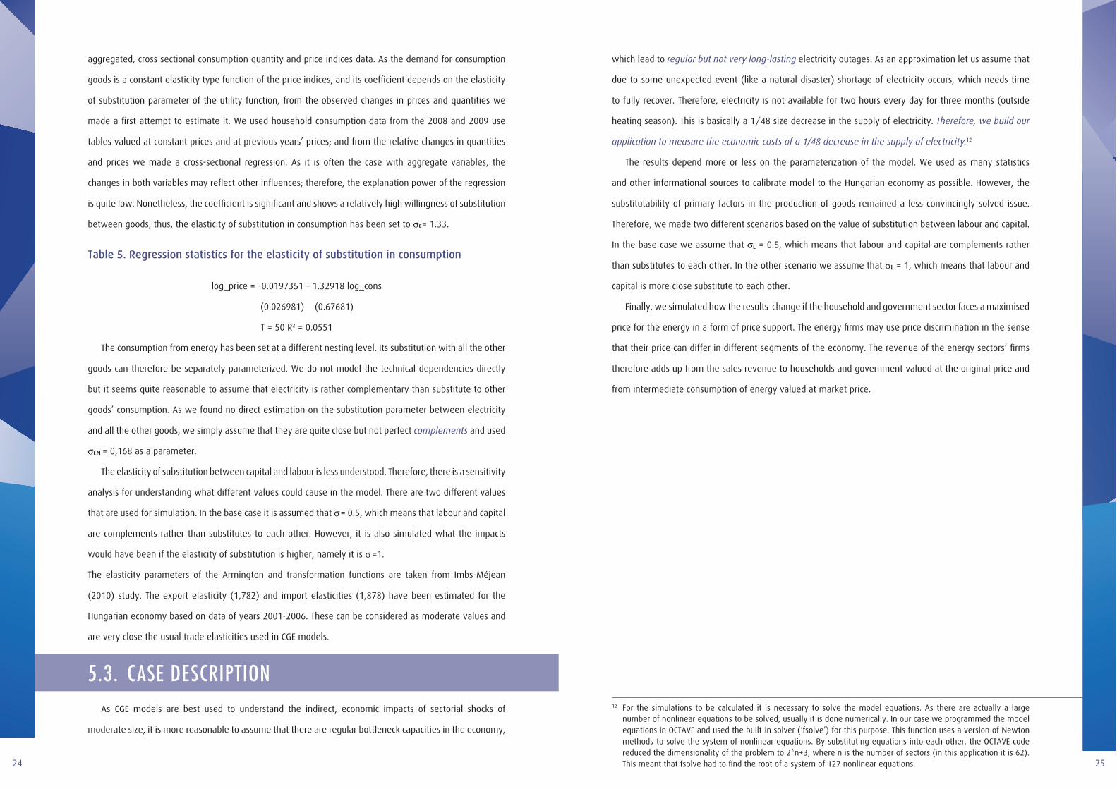
The elasticity of substitution between all (but the electricity) goods in consumption are estimated from
2524
aggregated, cross sectional consumption quantity and price indices data. As the demand for consumption
goods is a constant elasticity type function of the price indices, and its coefficient depends on the elasticity
of substitution parameter of the utility function, from the observed changes in prices and quantities we
made a first attempt to estimate it. We used household consumption data from the 2008 and 2009 use
tables valued at constant prices and at previous years’ prices; and from the relative changes in quantities
and prices we made a cross-sectional regression. As it is often the case with aggregate variables, the
changes in both variables may reflect other influences; therefore, the explanation power of the regression
is quite low. Nonetheless, the coefficient is significant and shows a relatively high willingness of substitution
between goods; thus, the elasticity of substitution in consumption has been set to σC= 1.33.
Table 5. Regression statistics for the elasticity of substitution in consumption
log_price = –0.0197351 – 1.32918 log_cons
(0.026981) (0.67681)
T = 50 R2 = 0.0551
The consumption from energy has been set at a different nesting level. Its substitution with all the other
goods can therefore be separately parameterized. We do not model the technical dependencies directly
but it seems quite reasonable to assume that electricity is rather complementary than substitute to other
goods’ consumption. As we found no direct estimation on the substitution parameter between electricity
and all the other goods, we simply assume that they are quite close but not perfect complements and used
σEN = 0,168 as a parameter.
The elasticity of substitution between capital and labour is less understood. Therefore, there is a sensitivity
analysis for understanding what different values could cause in the model. There are two different values
that are used for simulation. In the base case it is assumed that σ = 0.5, which means that labour and capital
are complements rather than substitutes to each other. However, it is also simulated what the impacts
would have been if the elasticity of substitution is higher, namely it is σ =1.
The elasticity parameters of the Armington and transformation functions are taken from Imbs-Méjean
(2010) study. The export elasticity (1,782) and import elasticities (1,878) have been estimated for the
Hungarian economy based on data of years 2001-2006. These can be considered as moderate values and
are very close the usual trade elasticities used in CGE models.
5.3. CASE DESCRIPTION As CGE models are best used to understand the indirect, economic impacts of sectorial shocks of
moderate size, it is more reasonable to assume that there are regular bottleneck capacities in the economy,
which lead to regular but not very long-lasting electricity outages. As an approximation let us assume that
due to some unexpected event (like a natural disaster) shortage of electricity occurs, which needs time
to fully recover. Therefore, electricity is not available for two hours every day for three months (outside
heating season). This is basically a 1/48 size decrease in the supply of electricity. Therefore, we build our
application to measure the economic costs of a 1/48 decrease in the supply of electricity.12
The results depend more or less on the parameterization of the model. We used as many statistics
and other informational sources to calibrate model to the Hungarian economy as possible. However, the
substitutability of primary factors in the production of goods remained a less convincingly solved issue.
Therefore, we made two different scenarios based on the value of substitution between labour and capital.
In the base case we assume that σL = 0.5, which means that labour and capital are complements rather
than substitutes to each other. In the other scenario we assume that σL = 1, which means that labour and
capital is more close substitute to each other.
Finally, we simulated how the results change if the household and government sector faces a maximised
price for the energy in a form of price support. The energy firms may use price discrimination in the sense
that their price can differ in different segments of the economy. The revenue of the energy sectors’ firms
therefore adds up from the sales revenue to households and government valued at the original price and
from intermediate consumption of energy valued at market price.
12 For the simulations to be calculated it is necessary to solve the model equations. As there are actually a large number of nonlinear equations to be solved, usually it is done numerically. In our case we programmed the model equations in OCTAVE and used the built-in solver (‘fsolve’) for this purpose. This function uses a version of Newton methods to solve the system of nonlinear equations. By substituting equations into each other, the OCTAVE code reduced the dimensionality of the problem to 2*n+3, where n is the number of sectors (in this application it is 62). This meant that fsolve had to find the root of a system of 127 nonlinear equations.
2726
6 . S IMUL AT ION RESULT S
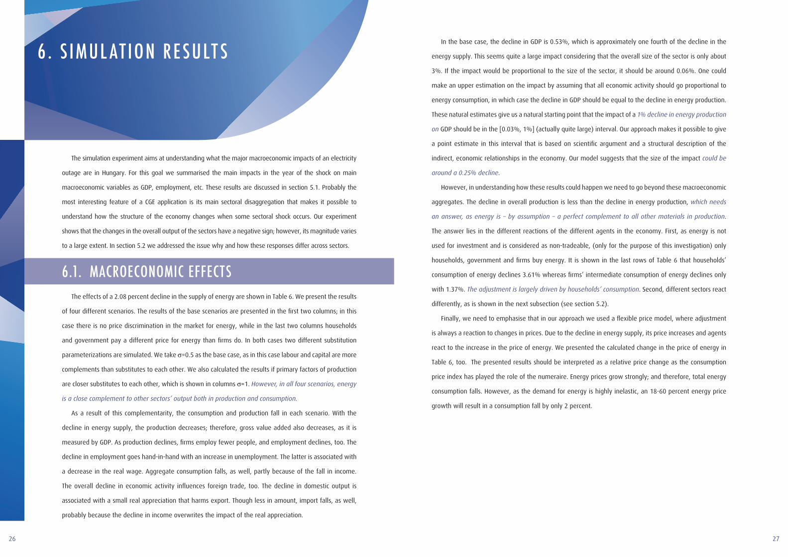
The simulation experiment aims at understanding what the major macroeconomic impacts of an electricity
outage are in Hungary. For this goal we summarised the main impacts in the year of the shock on main
macroeconomic variables as GDP, employment, etc. These results are discussed in section 5.1. Probably the
most interesting feature of a CGE application is its main sectoral disaggregation that makes it possible to
understand how the structure of the economy changes when some sectoral shock occurs. Our experiment
shows that the changes in the overall output of the sectors have a negative sign; however, its magnitude varies
to a large extent. In section 5.2 we addressed the issue why and how these responses differ across sectors.
6.1. MACROECONOMIC EFFECTS The effects of a 2.08 percent decline in the supply of energy are shown in Table 6. We present the results
of four different scenarios. The results of the base scenarios are presented in the first two columns; in this
case there is no price discrimination in the market for energy, while in the last two columns households
and government pay a different price for energy than firms do. In both cases two different substitution
parameterizations are simulated. We take σ=0.5 as the base case, as in this case labour and capital are more
complements than substitutes to each other. We also calculated the results if primary factors of production
are closer substitutes to each other, which is shown in columns σ=1. However, in all four scenarios, energy
is a close complement to other sectors’ output both in production and consumption.
As a result of this complementarity, the consumption and production fall in each scenario. With the
decline in energy supply, the production decreases; therefore, gross value added also decreases, as it is
measured by GDP. As production declines, firms employ fewer people, and employment declines, too. The
decline in employment goes hand-in-hand with an increase in unemployment. The latter is associated with
a decrease in the real wage. Aggregate consumption falls, as well, partly because of the fall in income.
The overall decline in economic activity influences foreign trade, too. The decline in domestic output is
associated with a small real appreciation that harms export. Though less in amount, import falls, as well,
probably because the decline in income overwrites the impact of the real appreciation.
In the base case, the decline in GDP is 0.53%, which is approximately one fourth of the decline in the
energy supply. This seems quite a large impact considering that the overall size of the sector is only about
3%. If the impact would be proportional to the size of the sector, it should be around 0.06%. One could
make an upper estimation on the impact by assuming that all economic activity should go proportional to
energy consumption, in which case the decline in GDP should be equal to the decline in energy production.
These natural estimates give us a natural starting point that the impact of a 1% decline in energy production
on GDP should be in the [0.03%, 1%] (actually quite large) interval. Our approach makes it possible to give
a point estimate in this interval that is based on scientific argument and a structural description of the
indirect, economic relationships in the economy. Our model suggests that the size of the impact could be
around a 0.25% decline.
However, in understanding how these results could happen we need to go beyond these macroeconomic
aggregates. The decline in overall production is less than the decline in energy production, which needs
an answer, as energy is – by assumption – a perfect complement to all other materials in production.
The answer lies in the different reactions of the different agents in the economy. First, as energy is not
used for investment and is considered as non-tradeable, (only for the purpose of this investigation) only
households, government and firms buy energy. It is shown in the last rows of Table 6 that households’
consumption of energy declines 3.61% whereas firms’ intermediate consumption of energy declines only
with 1.37%. The adjustment is largely driven by households’ consumption. Second, different sectors react
differently, as is shown in the next subsection (see section 5.2).
Finally, we need to emphasise that in our approach we used a flexible price model, where adjustment
is always a reaction to changes in prices. Due to the decline in energy supply, its price increases and agents
react to the increase in the price of energy. We presented the calculated change in the price of energy in
Table 6, too. The presented results should be interpreted as a relative price change as the consumption
price index has played the role of the numeraire. Energy prices grow strongly; and therefore, total energy
consumption falls. However, as the demand for energy is highly inelastic, an 18-60 percent energy price
growth will result in a consumption fall by only 2 percent.

2928
Table 6. Effects of a 2.08% decrease in the supply of energy in the year of the shock
Effects in the year of the shock
base casecase of price
discrimination
unit σ=0.5 σ=1 σ=0.5 σ=1
Macroeconomic variables
GDP % -0.53 -0.57 -0.90 -0.86
Employment % -0.84 -0.90 -1.40 -1.33
Unemployment rate %points 0.61 0.66 1.02 0.96
Real wage % -1.19 -1.27 -1.90 -1.81
Primary balance of government,
in % of GDP%points -0.29 -0.32 -0.46 -0.46
Consumption % -0.43 -0.40 -0.43 -0.38
Export % -1.02 -1.23 -2.11 -2.16
Import % -0.64 -0.77 -1.24 -1.30
Real exchange rate % -1.02 -0.84 -0.29 -0.13
Energy price and consumption
Real price of energy % 21.25 18.42 59.92* 46.52*
Households' consumption of
energy% -3.61 -3.20 -0.44 -0.38
Firms' consumption of energy % -1.37 -1.57 -2.88 -2.90
Total consumption of energy % -2.08 -2.08 -2.08 -2.08
*: change in the market price of energy that is paid by firms only.
The elasticity parameter of the primary factors had been chosen freely; therefore, we made simulations
for two different values to check how the results changes. As the table shows, there are no considerable
differences between the two specifications of the substitutability of primary factors of production. This is
not the case if there is price discrimination in the market for energy.
In the price discrimination scenario, households and government do not face with the shock of
higher energy prices; they pay the same price as before the shock. Therefore, they do not decrease their
consumption as much as in the base case. The decline turned out to be about 0.4 percent in our application.
Thus, firms will be “forced” to decrease their consumption of energy much more, which will result in a
higher decrease in production and employment. This basically means that the required decrease in the
demand for energy can only be reached by a much larger increase in the price of energy, as it can be seen
from the simulation results. It is important to note that the energy price change shown in the results table
is the price that firms pay in this scenario. Households’ price does not change – by assumption – in these
scenarios. Therefore, the average energy price what energy producing firms face is a weighted average.
We have shown earlier that intermediate consumption of energy is approximately two thirds of all energy
consumption; therefore, the average price of energy will increase by two-thirds of the price change we
presented in the table (40% and 31%, respectively).
In the case of price discrimination, the adjustment in the demand for energy is largely absorbed by
firms. This is resulted in a larger decrease in production, and thus a larger decrease in employment. The
real wage’s fall and the increase in the unemployment rate are larger in this specification. The contraction
of the economy is larger when firms are forced to decrease their energy consumption since it limits their
production possibilities.
6.2. SECTORIAL EFFECTS The changes in the sectors’ production are quite different from each other. It is reasonable to assume
that production will decline more in the energy-intensive industries. However, the adjustment in different
sectors might be influenced by other – but simultaneous – changes, as well. We have made a small analysis
to find out how the model specification (and the applied simplifications) and the nature of different sectors
are mutually responsible for the different reactions. The results are based on the simulation of the base
case (no price discrimination and labour and capital are not perfect complements in production).
The energy-intensity of the sectors is measured either by the share of energy in the total costs of
production (see Figure 3) or by the share of energy in the costs of intermediate inputs (see Figure 4).
As these are technological parameters, they are not influenced by the shock and are calculated from the
symmetric input-output tables. The figures show how these shares and the change in the sectors’ out-
put are related to each other in the simulation. As our results suggest, there are small differences in the
reactions of the tradeable and the non-tradeable sectors of the economy. We used different markers in the
graphs to illustrate that there are no differences in their energy-intensities on the average. The data of the
energy sector is not included in the figures as it is directly influenced by the shock.
3130
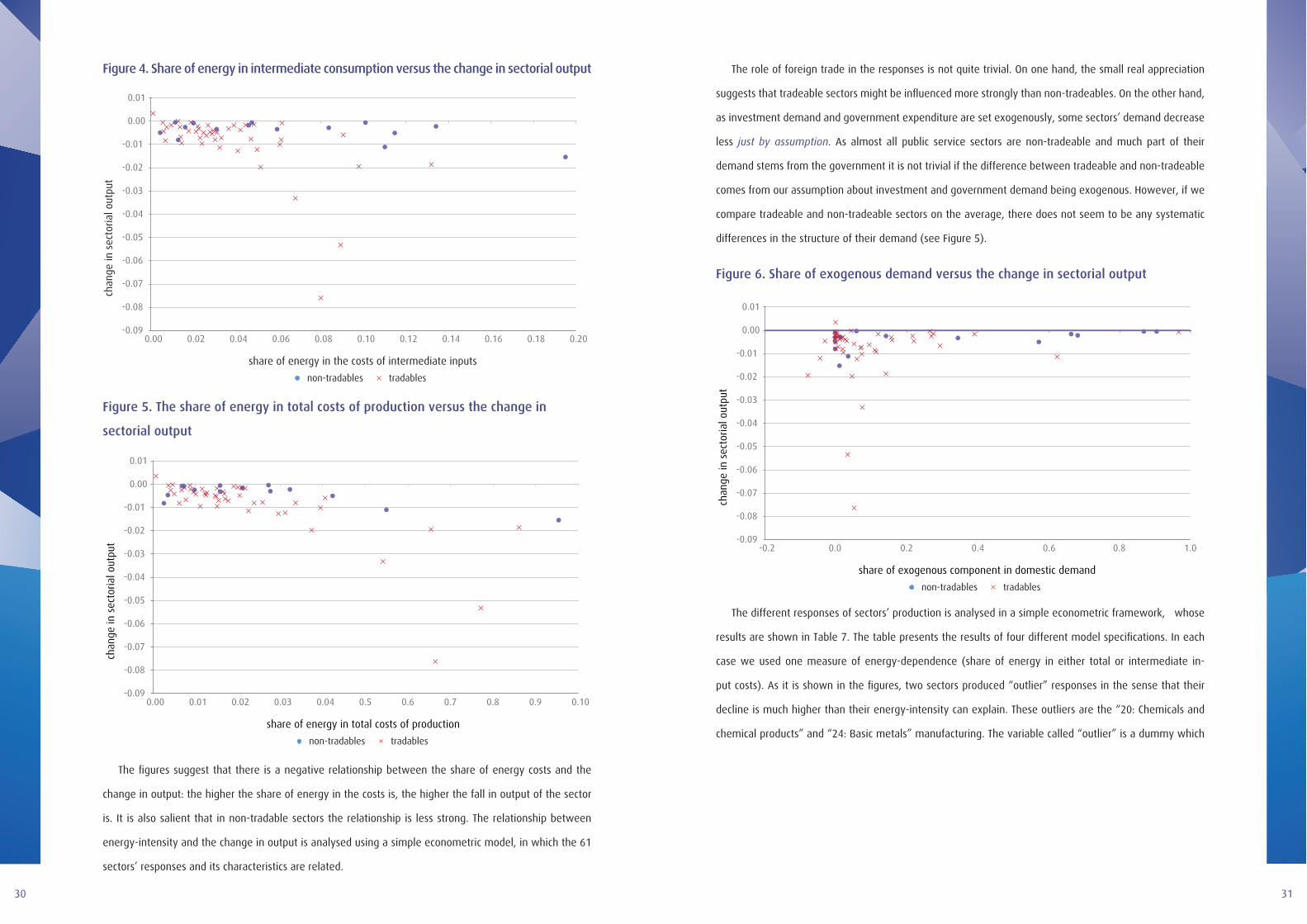
Figure 4. Share of energy in intermediate consumption versus the change in sectorial output
-0.09
-0.08
-0.07
-0.06
-0.05
-0.04
-0.03
-0.02
-0.01
0.00
0.01
0.00 0.02 0.04 0.06 0.08 0.10 0.12 0.14 0.16 0.18 0.20
chan
ge in
sec
toria
l out
put
share of energy in the costs of intermediate inputs
non-tradables tradables
Figure 5. The share of energy in total costs of production versus the change in
sectorial output
-0.09
-0.08
-0.07
-0.06
-0.05
-0.04
-0.03
-0.02
-0.01
0.00
0.01
0.00 0.01 0.02 0.03 0.04 0.5 0.6 0.7 0.8 0.9 0.10
chan
ge in
sec
toria
l out
put
share of energy in total costs of production
non-tradables tradables
The figures suggest that there is a negative relationship between the share of energy costs and the
change in output: the higher the share of energy in the costs is, the higher the fall in output of the sector
is. It is also salient that in non-tradable sectors the relationship is less strong. The relationship between
energy-intensity and the change in output is analysed using a simple econometric model, in which the 61
sectors’ responses and its characteristics are related.
The role of foreign trade in the responses is not quite trivial. On one hand, the small real appreciation
suggests that tradeable sectors might be influenced more strongly than non-tradeables. On the other hand,
as investment demand and government expenditure are set exogenously, some sectors’ demand decrease
less just by assumption. As almost all public service sectors are non-tradeable and much part of their
demand stems from the government it is not trivial if the difference between tradeable and non-tradeable
comes from our assumption about investment and government demand being exogenous. However, if we
compare tradeable and non-tradeable sectors on the average, there does not seem to be any systematic
differences in the structure of their demand (see Figure 5).
Figure 6. Share of exogenous demand versus the change in sectorial output
-0.09
-0.08
-0.07
-0.06
-0.05
-0.04
-0.03
-0.02
-0.01
0.00
0.01
-0.2 0.0 0.2 0.4 0.6 0.8 1.0
chan
ge in
sec
toria
l out
put
share of exogenous component in domestic demand
non-tradables tradables
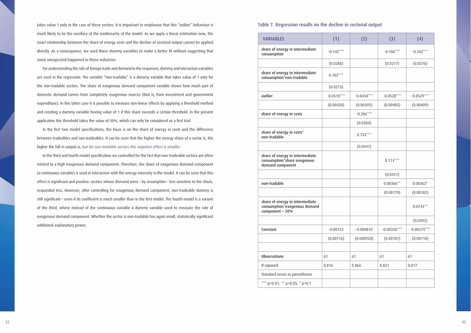
The different responses of sectors’ production is analysed in a simple econometric framework, whose
results are shown in Table 7. The table presents the results of four different model specifications. In each
case we used one measure of energy-dependence (share of energy in either total or intermediate in-
put costs). As it is shown in the figures, two sectors produced “outlier” responses in the sense that their
decline is much higher than their energy-intensity can explain. These outliers are the “20: Chemicals and
chemical products” and “24: Basic metals” manufacturing. The variable called “outlier” is a dummy which
3332
takes value 1 only in the case of these sectors. It is important to emphasise that this “outlier” behaviour is
much likely to be the corollary of the nonlinearity of the model. As we apply a linear estimation now, the
exact relationship between the share of energy costs and the decline of sectorial output cannot be applied
directly. As a consequence, we used these dummy variables to make a better fit without suggesting that
some unexpected happened in these industries.
For understanding the role of foreign trade and demand in the responses, dummy and interaction variables
are used in the regression. The variable “non-tradable” is a dummy variable that takes value of 1 only for
the non-tradable sectors. The share of exogenous demand component variable shows how much part of
domestic demand comes from completely exogenous sources (that is, from investment and government
expenditure). In this latter case it is possible to measure non-linear effects by applying a threshold method
and creating a dummy variable having value of 1 if this share exceeds a certain threshold. In the present
application this threshold takes the value of 50%, which can only be considered as a first trial.
In the first two model specifications, the focus is on the share of energy in costs and the difference
between tradeables and non-tradeables. It can be seen that the higher the energy share of a sector is, the
higher the fall in output is, but for non-tradable sectors this negative effect is smaller.
In the third and fourth model specification we controlled for the fact that non-tradeable sectors are often
related to a high exogenous demand component. Therefore, the share of exogenous demand component
(a continuous variable) is used in interaction with the energy-intensity in the model. It can be seen that this
effect is significant and positive: sectors whose demand were – by assumption – less sensitive to the shock,
responded less. However, after controlling for exogenous demand component, non-tradeable dummy is
still significant – even if its coefficient is much smaller than in the first model. The fourth model is a variant
of the third, where instead of the continuous variable a dummy variable used to measure the role of
exogenous demand component. Whether the sector is non-tradable has again small, statistically significant
additional explanatory power.
Table 7. Regression results on the decline in sectorial output
VARIABLES (1) (2) (3) (4)
share of energy in intermediate consumption
-0.143*** -0.106*** -0.102***
(0.0286) (0.0217) (0.0216)
share of energy in intermediate consumption*non-tradable
0.102***
(0.0273)
outlier -0.0510*** -0.0434*** -0.0528*** -0.0529***
(0.00420) (0.00393) (0.00405) (0.00409)
share of energy in costs -0.286***
(0.0384)
share of energy in costs*non-tradable
0.155***
(0.0441)
share of energy in intermediate consumption*share exogenous demand component
0.113***
(0.0417)
non-tradable 0.00366** 0.00363*
(0.00179) (0.00182)
share of energy in intermediate consumption*exogenous demand component > 50%
0.0743**
(0.0302)
Constant -0.00153 -0.000810 -0.00330*** -0.00315***
(0.00116) (0.000928) (0.00107) (0.00110)
Observations 61 61 61 61
R-squared 0.816 0.866 0.821 0.817
Standard errors in parentheses
*** p<0.01, ** p<0.05, * p<0.1

3534
The analysis has shown that there are rather large differences in the responses of the different sectors.
These differences largely related to the energy-intensity of the given sectors. However, the role of demand
is crucial, and will influence the responses to a large extent. Finally, it seems that non-tradeable sectors are
a bit less intensively influenced by this negative shock as they do not need to overcome the impacts of the
real appreciation.
CONCLUSIONS No doubt, energy, and especially electricity plays crucial role in the modern economies. Neither
production, nor consumption can be done without access to electricity. And even though it is hard to
imagine how to live without continuous access to electricity, regular or irregular outages could happen –
as it is actually the case sometimes. The damages and costs it may cause to the economies are hard to
measure; however, it is worth a try to understand how large these costs might be.
The advantage of a CGE application stems from the fact that – even though it is a highly abstract
approach without too many technological specifications – it makes it possible to understand how large
those indirect economic impacts can be. Indirect economic impacts exert their effects through the alteration
of prices, which also provides information about scarceness of goods. This application could not aim to
go into the very details of the micro environment, as how big part of a certain good can be consumed or
produced without access to energy. However, we assumed that energy is a close complement in both
production and consumption to other goods – moreover, it is a perfect complement to other intermediate
inputs and the primary inputs in production.
As a result of the complementarity assumption, we showed that a decline in the supply of energy leads
to a contraction of the economy that is much higher than the size of the sector would suggest – however, it
is not as much as it would be if all economy activities would be done in proportional to energy consumption.
This latter reasoning gives us a natural estimation that a 1% decline in the energy production should result a
decline of GDP somewhere in the [0.03%; 1%] interval (as the size of the energy producing sector is about
3% in Hungary). The simulation results showed that the size of the impact could be around a 0.25% decline.
It is important to understand what the adjustment mechanisms are behind this result. The decline
in overall production is less than the decline in energy production, which needs an answer, as energy
is – by assumption – a perfect complement to all other materials in production. The answer lies in the
different reactions of the different agents in the economy. As it turned out, the adjustment is largely driven
by households’ consumption. Also, we have shown that sectors with higher energy-intensive production
technologies decline more. Thus, the overall change of production is less than the change in the energy
supply. This is a kind of compound effect.
The different scenarios revealed that the size of the decline in GDP highly depends on which agents
react more drastically to the shock. In the base case, when prices are flexible and there are no limits to
adjustments, agents with the highest motivation to do so react more: either because their price-elasticity
is higher or because their energy intensity is higher or because they still need to compete with foreign
competitors. Therefore, this estimation must be considered as a lower bound on actual costs of electricity
outages: if there are limitations to adjustments of any kind, the GDP costs of the outage can be even higher.
This is illustrated with the scenario, when there is a special form of price discrimination in the market for
energy. When prices are distorted and do not reflect the actual scarceness of the goods, the adjustment will
cost more because it is not actors, who can do it at the lowest price, who respond more. We wish to emphasise
that the results come from a numerical simulation, which are to some extent sensitive to the values of the
parameters. Therefore, all numerical results should be interpreted conditional on the parameters that had been
chosen correctly. To our best knowledge these parameters fit to the available statistics of the Hungarian economy;
however, further improvement in the data background of any CGE model can never be an over-researched area.
Finally, we wish to point out that CGE models with their rich details about the industrial structure of the
economy are valuable tools to understand and measure how sectorial shocks will influence the economy,
how large the costs are related to certain sectorial specific shocks, and last but not least, how different
institutional arrangements could influence the impacts that these shocks unfold on the economy.
REFERENCESEbinger, Jane (2010): ECA Knowledge Brief: Albania’s Energy Sector: Vulnerable to Climate Change. Retrieved
from web.worldbank.org http://go.worldbank.org/AJM1XMWVV0
EBRD 2008: Albania Country Profile. B-a. Contracting Parties to the Treaty establishing the Energy Community.
September 2008. http://www.ebrd.com/downloads/legal/irc/countries/albania.pdf
Elôd, Fruzsina (19 August 2015): Mégis, miért nincs áram másfél napja több helyen? Retrieved from www.in-
dex.hu. Last downloaded on 6 October 2015. http://index.hu/belfold/budapest/2015/08/19/aramszunet/
Executive Office of the President (2013): Economic Benefits of Increasing Electric Grid Resilience to Weather
Outages. http://energy.gov/downloads/economic-benefits-increasing- electric-grid-resilience-weather-
outages. 2013 ACEEE Summer Study on Energy Efficiency in Industry
Guha, Gauri Shankar (2005): Simulation of the Economic Impact of Region-wide Electricity Outages from a
Natural Hazard Using a CGE Model. In: Southwestern Economic Review. vol. 2005 pp.101-124
IFC International Finance Corporation, World Bank Group 2013: Public-Private Partnership Impact Stories. Albania:
Ashta Hydropower. August 2013. Retrieved from www.ifc.org. http://www.ifc.org/wps/wcm/connect/e730
ce00498391aa858cd7336b93d75f/PPPImpactStories_Albania_AshtaHydropower.pdf?MOD=AJPERES

3736
Imbs, Jean & Isabelle Méjean (2010): Trade Elasticities: A Final Report for the European Commission, Euro-
pean Economy, Economic Papers 432, ec.europa.eu/economy_finance/publications
Keszthelyi, Krisztián (18 August 2015): Storm floods the streets of Budapest. Retrieved from www.bbj.hu, last
downloaded on 6 October 2015. http://bbj.hu/budapest/storm-floods-the-streets-of-budapest_102670
Kimura, Osamu & Ken-ichiro Nishio (2013): Saving Electricity in a Hurry: A Japanese Experience after the
Great East Japan Earthquake in 2011.I
Küster, Rober & Ingo Ellersdorfer & Ulrich Fahl (2007) A CGE-Analysis of Energy Policies Considering Labor
Market Imperfections and Technology Specifications. Climate Change and Sustainable Development Series,
January 2007, available at SSRN: http://ssrn.com/abstract=960725
MABISZ Magyar Biztosítók Szövetsége (24 August 2015) sajtóközlemény: Múlt hétfôi vihar: Eddig 13 ezer
kárbejelentés. Retrieved from: www.mabisz.hu, last downloaded on 6 October, 2015. http://www.mabisz.
hu/images/stories/docs/sajto/mabiszsajtotajekoztato20150824.pdf
Murakoshi, Chiharu & Hidetoshi Nakagami & Sho Hirayama (2012): Electricity Crisis and Behavior Change in
the Residential Sector: Tokyo Before and After the Great East Japan Earthquake. 2012 ACEEE Summer Study
on Energy Efficiency in Buildings
Pénzcentrum (19 August 2015). 5 ezer forintot kaphatnak az Elmû ügyfelei az áramszünet miatt. Retrieved
from www.penzcentrum.hu, last downloaded on 6 October 2015. http://www.penzcentrum.hu/otthon/5_
ezer_forintot_kaphatnak_az_elmu_ugyfelei_az_aramszunet_miatt.1046052.html
Reichl, Johannes & Michael Schmidthaler & Friedrich Schneider (2013): Power Outage Cost Evaluation:
Reasoning, Methods and an Application. In Journal of Scientific Research and Reports, 2013. 2(1): pp. 249-276.
Rose, Adam & Gbadebo Oladosu & Shu-Yi Liao (2007): Business Interruption Impacts of a Terrorist Attack
on the Electric Power System of Los Angeles: Customer Resilience to a Total Blackout. Published Articles &
Papers. Paper 68., 2007.
UCTE Final Report 2007, System Disturbance on 4 November 2006, Union for the Co-ordination of Transmission
of Electricity
W. Xie, N. Li, J-D.Wu & X-L. Hao (2014): Modeling the economic costs of disasters and recovery: analysis
using a dynamic computable general equilibrium model. In: Natural Hazards and Earth System Sciences, 14,
pp. 757-772, 2014
Webley, Kayla (26 November 2012): Hurricane Sandy By the Numbers: A Superstorm’s Statistics, One Month
Later. Retrieved from www.nation.time.com, last downloaded on 6 October 2015. http://nation.time.
com/2012/11/26/hurricane-sandy-one-month-later/

ABSZTRAK TA tanulmányban CGE modellt alkalmazunk a magyar gazdaságot érô szektorális sokkoknak a gazdasági
szereplôire és ágazataira gyakorolt hatásainak a vizsgálatára. A modellben az áramkimaradást az energia
kínálatának nem várt csökkenésével jelenítjük meg. Az energia ágazatban meglévô tôkeállomány nem várt
csökkenése vezet el az energia kínálatának csökkenéséhez. Feltesszük, hogy az energia mind a fogyasz-
tásban, mind a termelésben közeli kiegészítôje a többi ágazat termékeinek. Az kiindulópontnak tekintett
esetben az energia kínálatának 2,08%-os csökkenéséhez hatására a GDP 0,53%-al csökken. Ármerevségek
és más súrlódások, alkalmazkodási korlátok hiányában a sokkhoz történô alkalmazkodás nagy része azok-
hoz a szereplôkhöz köthetô, akik a legalacsonyabb költséggel tudják azt megtenni. Ezért ezt a becslést a
sokk okozta költségek egy alsó becslésének tekinthetjük. Alternatív szcenárió eredményein keresztül be-
mutatjuk, hogy ha az árak torzítottak, az áramkimaradás hatásai ennél nagyobbak is lehetnek.


