Using Rigging and Transfer to Animate 3D Characters by Ilya Baran B.S., Massachusetts Institute of Technology (2003) M.Eng., Massachusetts Institute of Technology (2004) MASSACHUSETTS INSTITUTE OF TECHNOLOGY OCT J 5 2010 L IBRARIES ARCHIVES Submitted to the Department of Electrical Engineering and Computer Science in partial fulfillment of the requirements for the degree of Doctor of Philosophy in Computer Science and Engineering at the MASSACHUSETTS INSTITUTE OF TECHNOLOGY September 2010 @ Massachusetts Institute of Technology 2010. All rights reserved. A uthor ...... w .......................... Department of Electrical Engineering and Computer Science Certified by....... August 18, 2010 Jovan Popovid Associate Professor Thesis Supervisor -7 Accepted by............. . . . ......................... Terry P. Orlando Chairman, Department Committee on Graduate Theses
Transcript
Using Rigging and Transfer to Animate 3D
Characters
by
Ilya Baran
B.S., Massachusetts Institute of Technology (2003)M.Eng., Massachusetts Institute of Technology (2004)
MASSACHUSETTS INSTITUTEOF TECHNOLOGY
OCT J 5 2010
L IBRARIES
ARCHIVES
Submitted to the Department of Electrical Engineering and ComputerScience
in partial fulfillment of the requirements for the degree of
Doctor of Philosophy in Computer Science and Engineering
at the
MASSACHUSETTS INSTITUTE OF TECHNOLOGY
September 2010
@ Massachusetts Institute of Technology 2010. All rights reserved.
A uthor ...... w ..........................Department of Electrical Engineering and Computer Science
Terry P. OrlandoChairman, Department Committee on Graduate Theses
2
Using Rigging and Transfer to Animate 3D Characters
by
Ilya Baran
Submitted to the Department of Electrical Engineering and Computer Scienceon August 18, 2010, in partial fulfillment of the
requirements for the degree ofDoctor of Philosophy in Computer Science and Engineering
Abstract
Transferring a mesh or skeletal animation onto a new mesh currently requires signif-icant manual effort. For skeletal animations, this involves rigging the character, byspecifying how the skeleton is positioned relative to the character and how posing theskeleton drives the character's shape. Currently, artists typically manually positionthe skeleton joints and paint skinning weights onto the character to associate pointson the character surface with bones. For this problem, we present a fully automaticrigging algorithm based on the geometry of the target mesh. Given a generic skeleton,the method computes both joint placement and the character surface attachment au-tomatically. For mesh animations, current techniques are limited to transferring themotion literally using a correspondence between the characters' surfaces. Instead, Ipropose an example-based method that can transfer motion between far more differ-ent characters and that gives the user more control over how to adapt the motion tothe new character.
Thesis Supervisor: Jovan PopovidTitle: Associate Professor
4
Acknowledgments
The biggest thanks goes to my advisor, Jovan Popovid. He was helpful and supportive
from the moment I asked him to take me as a student and even after he was no longer
at MIT. His guidance and flexibility made my graduate experience a pleasure.
The work in this thesis and outside was made possible by my collaborators, Daniel
Vlasic, Wojciech Matusik, Eitan Grinspun, and Jaakko Lehtinen. Thanks to them, I
learned to appreciate and enjoy the collaboration process.
A special thanks goes to Fredo Durand who often served as an informal second
advisor, providing valuable feedback and being generally friendly. Sylvain Paris has
also been extremely generous with writing help and sweets.
The MIT graphics group is a wonderful environment and I'd like to thank its mem-
bers for their friendship. From lunches to teabreaks to squash to pre-SIGGRRAPH
extreme hacking sessions, the graphics group is a great bunch. Although the friend-
ships will last, I will definitely miss the day-to-day interaction.
I would also like to thank my friends outside the graphics group whom I could
not see as often as I wanted to because of SIGGRAPH this or review that. There are
too many to list, but I will mention Leo Goldmakher, Lev, Anya, and Anya Teytel-
man, Esya and Max Kalashnikov, Misha Anikin, Anya and Sasha Giladi, Lera and
Dima Grinshpun, and Marina Zhurakhinskaya. Finally my thanks to my girlfriend
Angelique, my sister Inna, and my parents Roman and Elena, for their unconditional
A recent survey [12] describes and classifies many of the various methods. A curve-
skeleton can be used for skeletal animation and some algorithms for extracting a
............ NRIR .. .
curve-skeleton also compute a surface attachment [61, 35, 67]. While an extracted
curve-skeleton is a viable automatic rigging tool, it is hard to control its complexity
for characters with complex geometry. It also carries no semantic information, such
as which part of the extracted skeleton is an arm, and an existing animation therefore
cannot be directly applied.
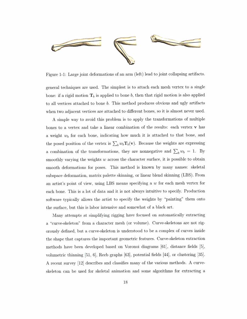
While linear blend skinning avoids the obvious discontinuities, it still suffers from
well-known problems. The fundamental issue is that linearly interpolating between a
0 degree rotation and a 180 degree rotation yields a singular matrix, rather than a 90
degree rotation. In practice, this leads to joint collapsing effects, as shown in Figure 1-
1. Artists get around this problem (as well as LBS's inability to capture muscle
bulges and other nonskeletal effects) by introducing more bones or using corrections
for certain poses. At the same time, there has been research work that aims to
address the drawbacks of linear blend skinning without increasing complexity. Some
recent work has attempted to improve on the quality of linear blend skinning, without
sacrificing real-time performance [37, 69, 36]. Within the same framework as LBS, i.e.,
mesh vertices attached to multiple bones with weights, the best current method is dual
quaternion blending [36], which avoids joint collapsing by combining transformations
in a way that preserves rigid motions.
However even without collapsing artifacts, the expressiveness of LBS is limited.
To capture non-skeletal effects, such as a bulging biceps, folding cloth, or skin sliding
over bone, several example-based methods have been developed [41, 40, 68]. The
drawback of such methods is, of course, that they require multiple example poses of
the character, which require artist effort to provide.
Recently, an alternative rigging method has become popular. Rather than em-
bedding a skeleton into the character, the character is itself embedded in a coarse
polyhedral cage. Each point of the character is expressed as a linear combination
of the cage vertices and deforming the cage results in the deformation of the char-
acter [17, 33, 32, 42]. Such methods have comparable deformation performance to
linear blend skinning, while avoiding joint collapses and allowing a greater freedom in
representing deformation. However, cages require careful construction and are more
difficult to control than skeletons.
A barrier to realism in the methods discussed above is that they are purely static:
the deformed surface at each point in time is a function of the control at that point
in time. In reality, however, the surface of a moving character is subject to temporal
effects like inertia. Animations that properly incorporate these effects tend to look
livelier and less stiff. There have been attempts to incorporate such physical effects
into animation rigs [10], but they reduce performance to levels unsuitable for computer
games, for example.
1.1.3 Animation
Controlling the degrees of freedom of a character poses another challenge. The two
most common approaches to this problem are motion capture and keyframing. A wide
variety of motion capture setups exist. In the majority of setups, an actor attaches
"markers" to different parts of his or her body and the motion capture system tracks
these markers and reconstructs the actor's skeletal motion. The markers may be active
or passive, optical, acoustic, inertial or magnetic. The captured motion can drive the
skeleton of a rigged model. Recently, a number of methods have been proposed to
capture the surface of an actor, not just his or her skeletal pose [57, 15, 66, 14]. This
allows capturing non-skeletal effects and even garment motion. These methods use
multiple synchronized video cameras to record a performance and process the video
to obtain a shape for each frame. In general, motion capture systems are expensive,
and often require a tedious clean-up step, but they can reproduce the actor's motion
with millimeter (or even better) precision.
While the primary benefit of motion capture is that it reproduces the motion of
the actor exactly, this can also be a drawback. Sometimes the virtual character needs
to move differently from how a human can move. When motion capture is available
and the desired motion is not far from what can be captured, editing tools exist for
both skeletal [21] and mesh [39] animation. In other cases, however, motion needs to
be created from scratch and keyframing is used. Keyframing involves specifying the
relevant degrees of freedom explicitly at certain points in time and interpolating to
get a smooth trajectory. Keyframing provides maximum flexibility, but is very labor
intensive and requires a great deal of artistic skill. As a result, several alternatives
have been proposed, mainly for simple models and motions. Sketching [62] or stylized
acting [16] provide simple input methods. Placing keyframes in a space other than the
timeline leads to spatial keyframing [29] or (in the case of 2D characters) configuration
modeling [50].
In some cases, it is possible to embed the character in a simulated physical environ-
ment and either use a controller to drive the character's skeleton [65, 52, 23, 74, 13],
or use spacetime optimization to find a motion that optimizes some objective (such
as minimizing energy expenditure), while respecting physical laws [73, 49]. These
techniques are rarely used in practice because constructing robust controllers that
produce believable motion is very difficult and spacetime optimization is very high-
dimensional and therefore slow and unstable.
To obtain more sophisticated animations with less work than keyframing or phys-
ical simulation, several methods for reusing existing motion have been proposed. For
skeletal motion, methods exist for retargetting to new characters [20], changing the
style [25], mapping to completely new motion [24], or learning a probabilistic model
that can synthesize new motion automatically [8].
For mesh animation, as opposed to skeletal animation, there has been less work
on reusing motion. The only method developed to date specifically for this purpose
is deformation transfer [58]. It uses a correspondence between the surfaces of two
characters to transfer the motion of one character onto another. However, the char-
acters on which this works need to be similar, providing the surface correspondence
may be difficult, and the motion is transferred without modification. Our work aims
to address these drawbacks.
1.2 Contributions
This thesis presents two algorithms designed to simplify character animation. The
first algorithm, automatic rigging, enables skeletal rigging to be done fully automati-
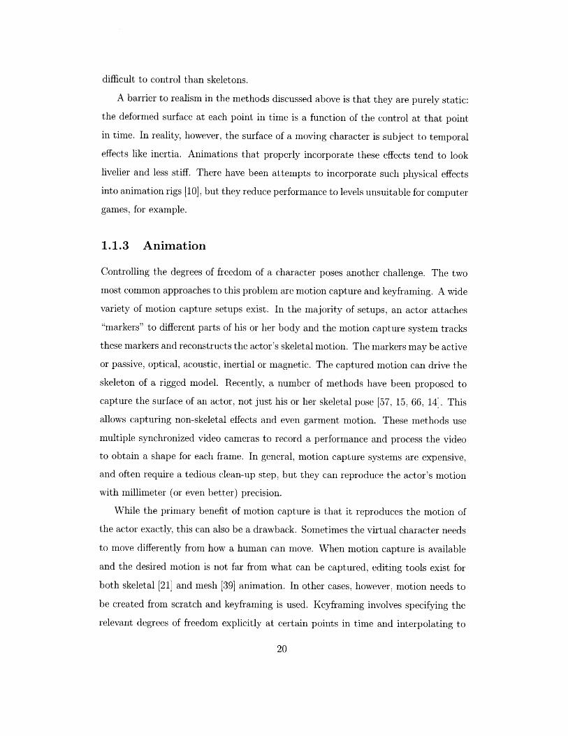
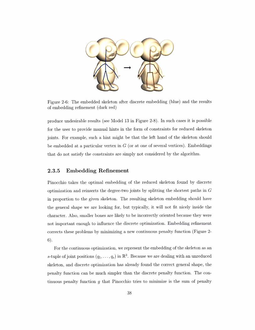
Figure 1-2: The automatic rigging method presented in this thesis allowed us toimplement an easy-to-use animation system, which we called Pinocchio. In this ex-ample, the triangle mesh of a jolly cartoon character is brought to life by embeddinga skeleton inside it and applying a walking motion to the initially static shape.
cally, allowing a user to apply an existing skeletal animation to a new character. The
second algorithm, semantic deformation transfer, expands the class of mesh anima-
tions that is possible to obtain from existing mesh animations.
1.2.1 Automatic Rigging
While recent modeling techniques have made the creation of 3D characters accessible
to novices and children, bringing these static shapes to life is still not easy. In a
conventional skeletal animation package, the user must rig the character manually.
This requires placing the skeleton joints inside the character and specifying which
parts of the surface are attached to which bone. The tedium of this process makes
simple character animation difficult.
We present a system that eliminates this tedium to make animation more acces-
sible for children, educators, researchers, and other non-expert animators. A design
.................................... ..
goal is for a child to be able to model a unicorn, click the "Quadruped Gallop" but-
ton, and watch the unicorn start galloping. To support this functionality, we need a
method (as shown in Figure 1-2) that takes a character, a skeleton, and a motion of
that skeleton as input, and outputs the moving character.
1.2.2 Semantic Deformation Transfer
When a skeletal model cannot adequately capture the desired complexity of the de-
formation, reusing existing mesh animations to drive new ones is an attractive alter-
native. Existing methods apply when a surface correspondence is defined between the
characters and the characters move in the same manner. While existing techniques
can map a horse motion to a camel motion, they cannot, for example, transfer motion
from a human to a flamingo, because the knees bend in a different direction. To sup-
port transferring mesh animation to very different characters, we developed semantic
deformation transfer, which preserves the semantics of the motion, while adapting
it to the target character. The user provides several pairs of example poses that
exercise the relevant degrees of freedom to specify semantic correspondence between
two characters. For example, to transform a human walk onto a flamingo, the user
needs to provide poses of the human with bent knees and corresponding poses of the
flamingo with knees bent backwards. The algorithm then learns a mapping between
the two characters that could then be applied to new motions. Semantic deformation
transfer can also be seen as a generalization of keyframing, in which keyframes are
placed in the source character's pose space.
24
Chapter 2
Automatic Rigging
2.1 Overview
Our automatic rigging algorithm consists of two main steps: skeleton embedding and
skin attachment. Skeleton embedding computes the joint positions of the skeleton
inside the character by minimizing a penalty function. To make the optimization
problem computationally feasible, we first embed the skeleton into a discretization of
the character's interior and then refine this embedding using continuous optimization.
The skin attachment is computed by assigning bone weights based on the proximity of
the embedded bones smoothed by a diffusion equilibrium equation over the character's
surface.
Our design decisions relied on three criteria, which we also used to evaluate our
system:
" Generality: A single skeleton is applicable to a wide variety of characters: for
example, our method can use a generic biped skeleton to rig an anatomically
correct human model, an anthropomorphic robot, and even something that has
very little resemblance to a human.
" Quality: The resulting animation quality is comparable to that of modern
video games.
" Performance: The automatic rigging usually takes under one minute on an
everyday PC.
A key design challenge is constructing a penalty function that penalizes unde-
sirable embeddings and generalizes well to new characters. For this, we designed a
maximum-margin supervised learning method to combine a set of hand-constructed
penalty functions. To ensure an honest evaluation and avoid overfitting, we tested
our algorithm on 16 characters that we did not see or use during development. Our
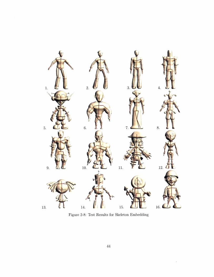
algorithm computed a good rig for all but 3 of these characters. For each of the
remaining cases, one joint placement hint corrected the problem.
We simplify the problem by making the following assumptions. The character
mesh must be the boundary of a connected volume. The character must be given in
approximately the same orientation and pose as the skeleton. Lastly, the character
must be proportioned roughly like the given skeleton.
We introduce several new techniques to solve the automatic rigging problem:
" A maximum-margin method for learning the weights of a linear combination
of penalty functions based on examples, as an alternative to hand-tuning (Sec-
tion 2.3.3).
" An A*-like heuristic to accelerate the search for an optimal skeleton embedding
over an exponential search space (Section 2.3.4).
" The use of Laplace's diffusion equation to generate weights for attaching mesh
vertices to the skeleton using linear blend skinning (Section 2.4). This method
can also be useful in existing 3D packages when the skeleton is manually em-
bedded.
Our prototype system, called Pinocchio, rigs the given character using our algo-
rithm. It then transfers a motion to the character using online motion retargetting [11]
to eliminate footskate by constraining the feet trajectories of the character to the feet
trajectories of the given motion.
2.2 Related Work
Character Animation Most prior research in character animation, especially in
3D, has focused on professional animators; very little work is targeted at novice users.
Recent exceptions include Motion Doodles [62] as well as the work of Igarashi et al.
on spatial keyframing [29] and as-rigid-as-possible shape manipulation [28]. These
approaches focus on simplifying animation control, rather than simplifying the defi-
nition of the articulation of the character. In particular, a spatial keyframing system
expects an articulated character as input, and as-rigid-as-possible shape manipula-
tion, besides being 2D, relies on the constraints to provide articulation information.
The Motion Doodles system has the ability to infer the articulation of a 2D charac-
ter, but their approach relies on very strong assumptions about how the character is
presented.
Some previous techniques for character animation infer articulation from multiple
example meshes [40]. Given sample meshes, mesh-based inverse kinematics [59] con-
structs a nonlinear model of meaningful mesh configurations, while James and Twigg
[30] construct a linear blend skinning model, albeit without a meaningful hierarchical
skeleton. However, such techniques are unsuitable for our problem because we only
have a single mesh. We obtain the character articulation from the mesh by using the
given skeleton not just as an animation control structure, but also as an encoding of
the likely modes of deformation.
Skeleton Extraction Although most skeleton-based prior work on automatic rig-
ging focused on skeleton extraction, for our problem, we advocate skeleton embedding.
A few approaches to the skeleton extraction problem are representative. Teichmann
and Teller [61] extract a skeleton by simplifying the Voronoi skeleton with a small
amount of user assistance. Liu et al. [44] use repulsive force fields to find a skeleton.
In their paper, Katz and Tal [35] describe a surface partitioning algorithm and sug-
gest skeleton extraction as an application. The technique in Wade [67] is most similar
to our own: like us, they approximate the medial surface by finding discontinuities in
the distance field, but they use it to construct a skeleton tree.
For the purpose of automatically animating a character, however, skeleton embed-
ding is much more suitable than extraction. For example, the user may have motion
data for a quadruped skeleton, but extracting the skeleton from the geometry of a
complicated quadruped character, is likely to lead to an incompatible skeleton topol-
ogy. The anatomically appropriate skeleton generation by Wade [67] ameliorates this
problem by techniques such as identifying appendages and fitting appendage tem-
plates, but the overall topology of the resulting skeleton may still vary. For example,
for the character in Figure 1-2, ears may be mistaken for arms. Another advantage of
embedding over extraction is that the given skeleton provides information about the
expected structure of the character, which may be difficult to obtain from just the
geometry. So although we could use an existing skeleton extraction algorithm and
embed our skeleton into the extracted one, the results would likely be undesirable.
For example, the legs of the character in Figure 1-2 would be too short if a skeleton
extraction algorithm were used.
Template Fitting Animating user-provided data by fitting a template has been
successful in cases when the model is fairly similar to the template. Most of the work
has been focused on human models, making use of human anatomy specifics, e.g.
[47]. For segmenting and animating simple 3D models of characters and inanimate
objects, Anderson et al. [1] fit voxel-based volumetric templates to the data.
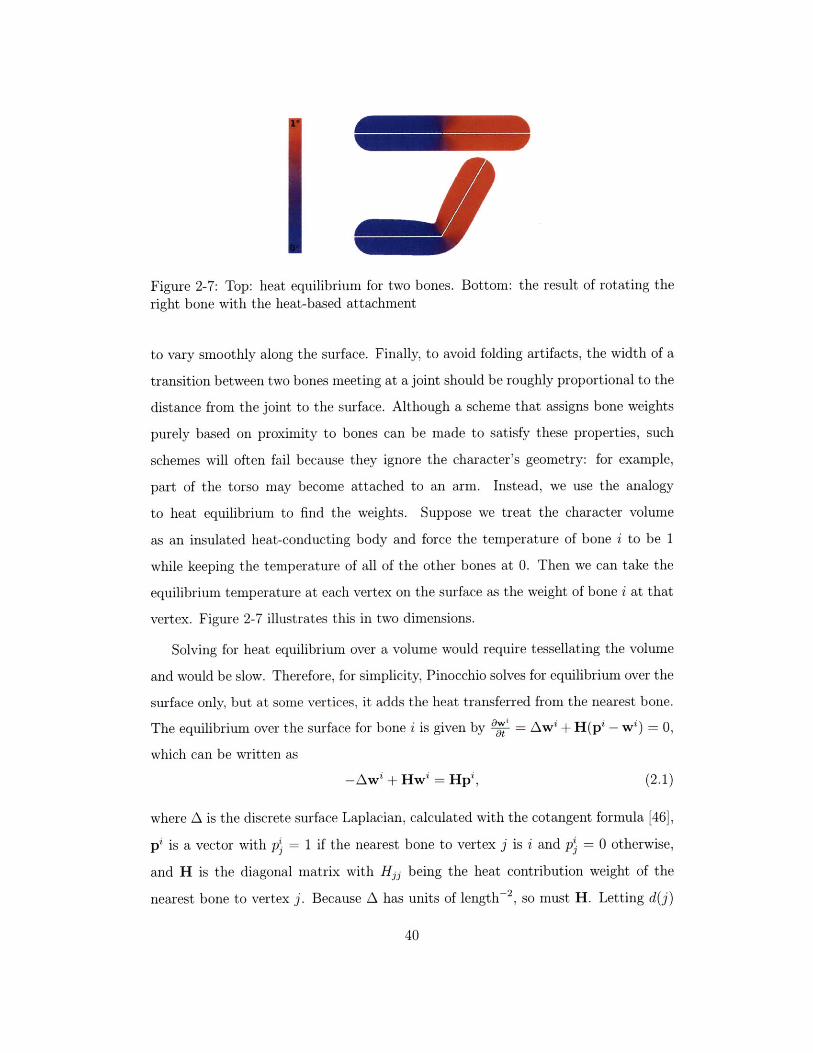
Skinning Almost any system for mesh deformation (whether surface based [43, 75]
or volume based [76]) can be adapted for skeleton-based deformation. Teichmann
and Teller [61] propose a spring-based method. Unfortunately, at present, these
methods are unsuitable for real-time animation of even moderate size meshes. Because
of its simplicity and efficiency (and simple GPU implementation), and despite its
quality shortcomings, linear blend skinning (LBS), also known as skeleton subspace
deformation, remains the most popular method used in practice.
Most real-time skinning work, e.g. [40, 68], has focused on improving on LBS
by inferring the character articulation from multiple example meshes. However, such
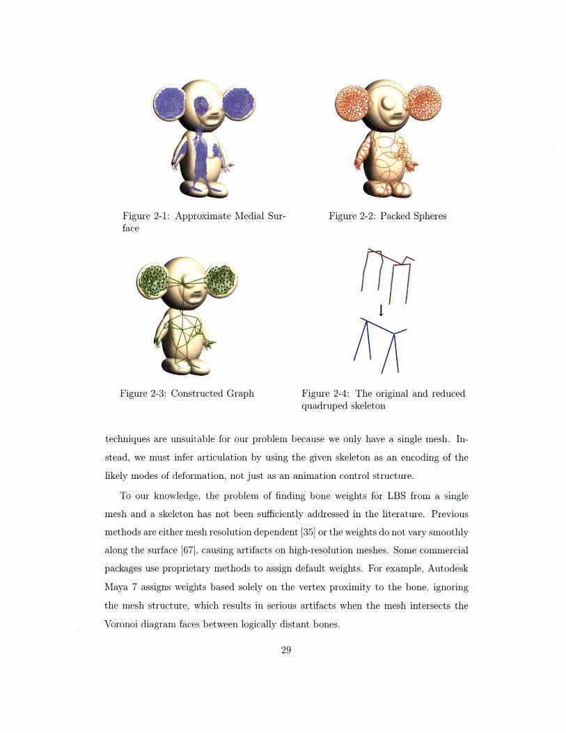
Figure 2-1:face
Approximate Medial Sur-
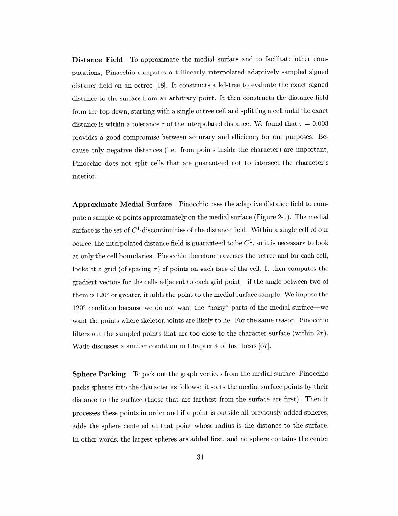
Figure 2-3: Constructed Graph
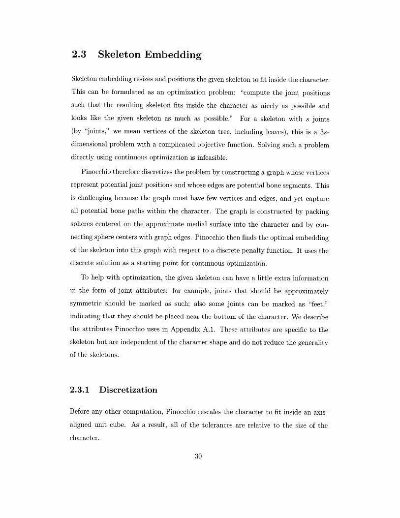
Figure 2-2: Packed Spheres
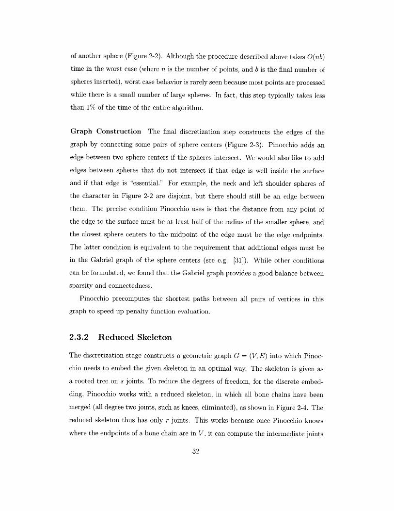
Figure 2-4: The original and reducedquadruped skeleton
techniques are unsuitable for our problem because we only have a single mesh. In-
stead, we must infer articulation by using the given skeleton as an encoding of the
likely modes of deformation, not just as an animation control structure.
To our knowledge, the problem of finding bone weights for LBS from a single
mesh and a skeleton has not been sufficiently addressed in the literature. Previous
methods are either mesh resolution dependent [35] or the weights do not vary smoothly
along the surface [67], causing artifacts on high-resolution meshes. Some commercial
packages use proprietary methods to assign default weights. For example, Autodesk
Maya 7 assigns weights based solely on the vertex proximity to the bone, ignoring
the mesh structure, which results in serious artifacts when the mesh intersects the
Voronoi diagram faces between logically distant bones.
. . .............. .
2.3 Skeleton Embedding
Skeleton embedding resizes and positions the given skeleton to fit inside the character.
This can be formulated as an optimization problem: "compute the joint positions
such that the resulting skeleton fits inside the character as nicely as possible and
looks like the given skeleton as much as possible." For a skeleton with s joints
(by "joints," we mean vertices of the skeleton tree, including leaves), this is a 3s-
dimensional problem with a complicated objective function. Solving such a problem
directly using continuous optimization is infeasible.
Pinocchio therefore discretizes the problem by constructing a graph whose vertices
represent potential joint positions and whose edges are potential bone segments. This
is challenging because the graph must have few vertices and edges, and yet capture
all potential bone paths within the character. The graph is constructed by packing
spheres centered on the approximate medial surface into the character and by con-
necting sphere centers with graph edges. Pinocchio then finds the optimal embedding
of the skeleton into this graph with respect to a discrete penalty function. It uses the
discrete solution as a starting point for continuous optimization.
To help with optimization, the given skeleton can have a little extra information
in the form of joint attributes: for example, joints that should be approximately
symmetric should be marked as such; also some joints can be marked as "feet,"
indicating that they should be placed near the bottom of the character. We describe
the attributes Pinocchio uses in Appendix A.1. These attributes are specific to the
skeleton but are independent of the character shape and do not reduce the generality
of the skeletons.
2.3.1 Discretization
Before any other computation, Pinocchio rescales the character to fit inside an axis-
aligned unit cube. As a result, all of the tolerances are relative to the size of the
character.
Distance Field To approximate the medial surface and to facilitate other com-
putations, Pinocchio computes a trilinearly interpolated adaptively sampled signed
distance field on an octree [18]. It constructs a kd-tree to evaluate the exact signed
distance to the surface from an arbitrary point. It then constructs the distance field
from the top down, starting with a single octree cell and splitting a cell until the exact
distance is within a tolerance T of the interpolated distance. We found that T= 0.003
provides a good compromise between accuracy and efficiency for our purposes. Be-
cause only negative distances (i.e. from points inside the character) are important,
Pinocchio does not split cells that are guaranteed not to intersect the character's
interior.
Approximate Medial Surface Pinocchio uses the adaptive distance field to com-
pute a sample of points approximately on the medial surface (Figure 2-1). The medial
surface is the set of C1 -discontinuities of the distance field. Within a single cell of our
octree, the interpolated distance field is guaranteed to be C1 , so it is necessary to look
at only the cell boundaries. Pinocchio therefore traverses the octree and for each cell,
looks at a grid (of spacing T) of points on each face of the cell. It then computes the
gradient vectors for the cells adjacent to each grid point-if the angle between two of
them is 120' or greater, it adds the point to the medial surface sample. We impose the
120' condition because we do not want the "noisy" parts of the medial surface-we
want the points where skeleton joints are likely to lie. For the same reason, Pinocchio
filters out the sampled points that are too close to the character surface (within 2T).
Wade discusses a similar condition in Chapter 4 of his thesis [67].
Sphere Packing To pick out the graph vertices from the medial surface, Pinocchio
packs spheres into the character as follows: it sorts the medial surface points by their
distance to the surface (those that are farthest from the surface are first). Then it
processes these points in order and if a point is outside all previously added spheres,
adds the sphere centered at that point whose radius is the distance to the surface.
In other words, the largest spheres are added first, and no sphere contains the center
of another sphere (Figure 2-2). Although the procedure described above takes O(nb)
time in the worst case (where n is the number of points, and b is the final number of
spheres inserted), worst case behavior is rarely seen because most points are processed
while there is a small number of large spheres. In fact, this step typically takes less
than 1% of the time of the entire algorithm.
Graph Construction The final discretization step constructs the edges of the
graph by connecting some pairs of sphere centers (Figure 2-3). Pinocchio adds an
edge between two sphere centers if the spheres intersect. We would also like to add
edges between spheres that do not intersect if that edge is well inside the surface
and if that edge is "essential." For example, the neck and left shoulder spheres of
the character in Figure 2-2 are disjoint, but there should still be an edge between
them. The precise condition Pinocchio uses is that the distance from any point of
the edge to the surface must be at least half of the radius of the smaller sphere, and
the closest sphere centers to the midpoint of the edge must be the edge endpoints.
The latter condition is equivalent to the requirement that additional edges must be
in the Gabriel graph of the sphere centers (see e.g. [31]). While other conditions
can be formulated, we found that the Gabriel graph provides a good balance between
sparsity and connectedness.
Pinocchio precomputes the shortest paths between all pairs of vertices in this
graph to speed up penalty function evaluation.
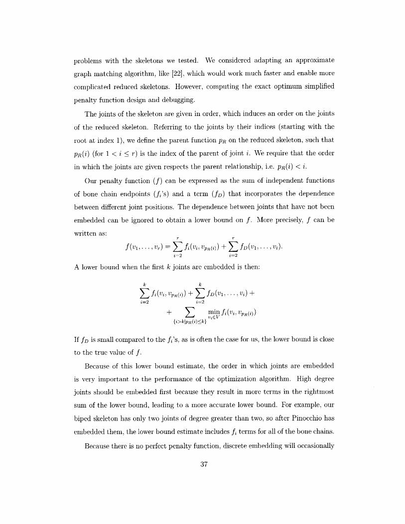
2.3.2 Reduced Skeleton
The discretization stage constructs a geometric graph G = (V, E) into which Pinoc-
chio needs to embed the given skeleton in an optimal way. The skeleton is given as
a rooted tree on s joints. To reduce the degrees of freedom, for the discrete embed-
ding, Pinocchio works with a reduced skeleton, in which all bone chains have been
merged (all degree two joints, such as knees, eliminated), as shown in Figure 2-4. The
reduced skeleton thus has only r joints. This works because once Pinocchio knows
where the endpoints of a bone chain are in V, it can compute the intermediate joints
by taking the shortest path between the endpoints and splitting it in accordance with
the proportions of the unreduced skeleton. For the humanoid skeleton we use, for
example, s = 18, but r = 7; without a reduced skeleton, the optimization problem
would typically be intractable.
Therefore, the discrete skeleton embedding problem is to find the embedding of
the reduced skeleton into G, represented by an r-tuple v = (v1,..., vr) of vertices in
V, which minimizes a penalty function f(v) that is designed to penalize differences
in the embedded skeleton from the given skeleton.
2.3.3 Discrete Penalty Function
The discrete penalty function has great impact on the generality and quality of the
results. A good embedding should have the proportions, bone orientations, and size
similar to the given skeleton. The paths representing the bone chains should be
disjoint, if possible. Joints of the skeleton may be marked as "feet," in which case
they should be close to the bottom of the character. Designing a penalty function
that satisfies all of these requirements simultaneously is difficult. Instead we found it
easier to design penalties independently and then rely on learning a proper weighting
for a global penalty that combines each term.
The Setup We represent the penalty function f as a linear combination of k "basis"
penalty functions: f (v) = Z 1 -yib(v). Pinocchio uses k = 9 basis penalty functions
constructed by hand. They penalize short bones, improper orientation between joints,
length differences in bones marked symmetric, bone chains sharing vertices, feet away
from the bottom, zero-length bone chains, improper orientation of bones, degree-one
joints not embedded at extreme vertices, and joints far along bone-chains but close in
the graph (see Appendix A.2 for details). We determine the weights F = (-Y1, ... 7, y)
semi-automatically via a new maximum margin approach inspired by support vector
machines.
Suppose that for a single character, we have several example embeddings, each
marked "good" or "bad". The basis penalty functions assign a feature vector b(v) =
(bi(v), . . . , bk (v)) to each example embedding v. Let pi, . . . , pm be the k-dimensional
feature vectors of the good embeddings and let q1,... q, be the feature vectors of
the bad embeddings.
Maximum Margin To provide context for our approach, we review the relevant
ideas from the theory of support vector machines. See Burges [9] for a much more
complete tutorial. If our goal were to automatically classify new embeddings into
"good" and "bad" ones, we could use a support vector machine to learn a maximum
margin linear classifier. In its simplest form, a support vector machine finds the hy-
perplane that separates the pi's from the qi's and is as far away from them as possible.
More precisely, if F is a k-dimensional vector with ||F|| = 1, the classification margin
of the best hyperplane normal to F is 1 (minti fTq1 - maxi FTp2 ). Recalling that
the total penalty of an embedding v is FTb(v), we can think of the maximum margin
F as the one that best distinguishes between the best "bad" embedding and the worst
"good" embedding in the training set.
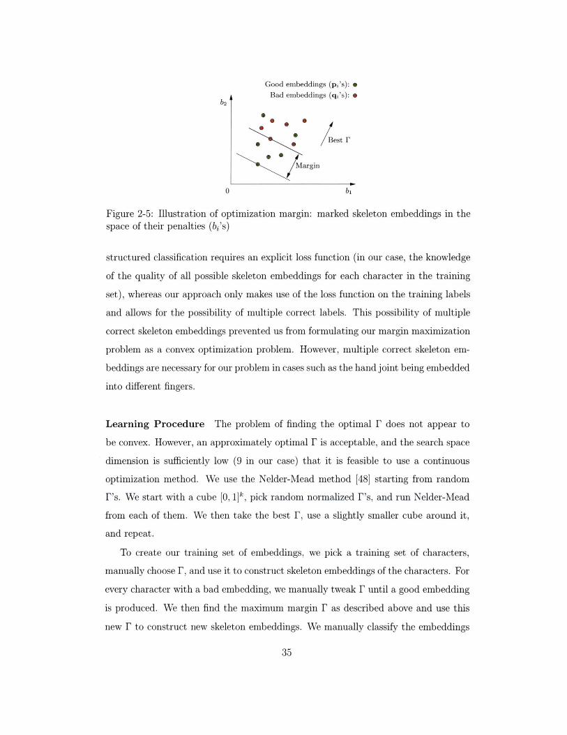
In our case, however, we do not need to classify embeddings, but rather find a F
such that the embedding with the lowest penalty f(v) = FTb(v) is likely to be good.
To this end, we want F to distinguish between the best "bad" embedding and the
best "good" embedding, as illustrated in Figure 2-5. We therefore wish to maximize
the optimization margin (subject to ||F7| = 1), which we define as:
min FTqi - min FTp.i=1 i=1
Because we have different characters in our training set, and because the embedding
quality is not necessarily comparable between different characters, we find the F that
maximizes the minimum margin over all of the characters.
Our approach is similar to margin-based linear structured classification [60], the
problem of learning a classifier that to each problem instance (cf. character) assigns
the discrete label (cf. embedding) that minimizes the dot product of a weights vector
with basis functions of the problem instance and label. The key difference is that
Good embeddings (pt's): e
b2 'Bad embeddings (qi's): e
00
/Best f
Margin
0 b1
Figure 2-5: Illustration of optimization margin: marked skeleton embeddings in thespace of their penalties (bi's)
structured classification requires an explicit loss function (in our case, the knowledge
of the quality of all possible skeleton embeddings for each character in the training
set), whereas our approach only makes use of the loss function on the training labels
and allows for the possibility of multiple correct labels. This possibility of multiple
correct skeleton embeddings prevented us from formulating our margin maximization
problem as a convex optimization problem. However, multiple correct skeleton em-
beddings are necessary for our problem in cases such as the hand joint being embedded
into different fingers.
Learning Procedure The problem of finding the optimal F does not appear to
be convex. However, an approximately optimal F is acceptable, and the search space
dimension is sufficiently low (9 in our case) that it is feasible to use a continuous
optimization method. We use the Nelder-Mead method [48] starting from random
F's. We start with a cube [0, 1]', pick random normalized F's, and run Nelder-Mead
from each of them. We then take the best F, use a slightly smaller cube around it,
and repeat.
To create our training set of embeddings, we pick a training set of characters,
manually choose F, and use it to construct skeleton embeddings of the characters. For
every character with a bad embedding, we manually tweak F until a good embedding
is produced. We then find the maximum margin F as described above and use this
new F to construct new skeleton embeddings. We manually classify the embeddings
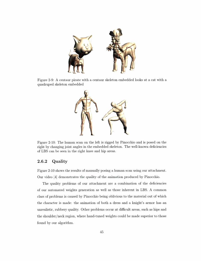
Figure 2-9: A centaur pirate with a centaur skeleton embedded looks at a cat with aquadruped skeleton embedded
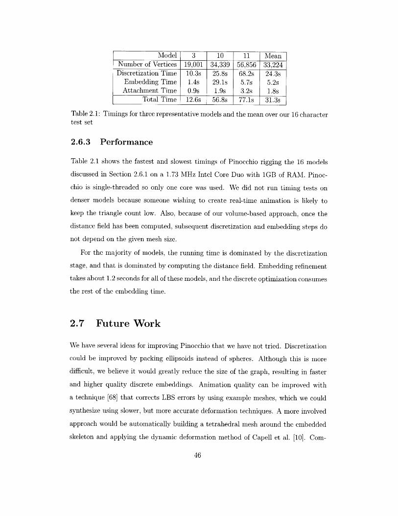
Figure 2-10: The human scan on the left is rigged by Pinocchio and is posed on theright by changing joint angles in the embedded skeleton. The well-known deficienciesof LBS can be seen in the right knee and hip areas.
2.6.2 Quality
Figure 2-10 shows the results of manually posing a human scan using our attachment.
Our video [4] demonstrates the quality of the animation produced by Pinocchio.
The quality problems of our attachment are a combination of the deficiencies
of our automated weights generation as well as those inherent in LBS. A common
class of problems is caused by Pinocchio being oblivious to the material out of which
the character is made: the animation of both a dress and a knight's armor has an
unrealistic, rubbery quality. Other problems occur at difficult areas, such as hips and
the shoulder/neck region, where hand-tuned weights could be made superior to those
found by our algorithm.
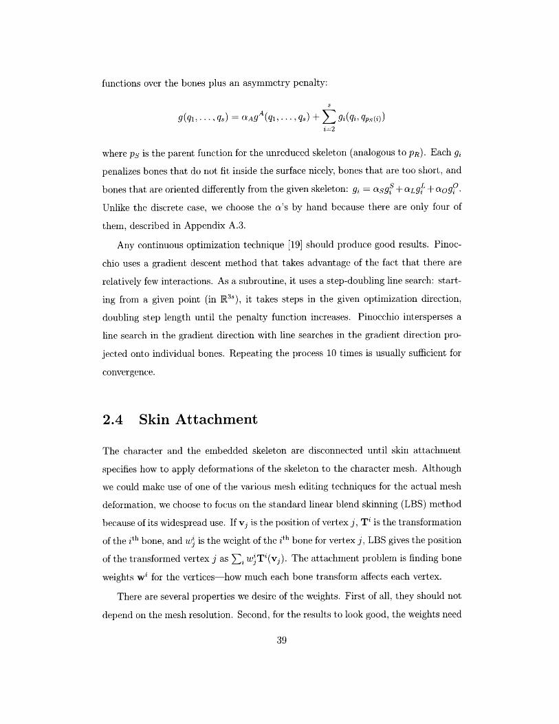
...........
Model 3 10 11 MeanNumber of Vertices 19,001 34,339 56,856 33,224Discretization Time 10.3s 25.8s 68.2s 24.3s
Embedding Time 1.4s 29.1s 5.7s 5.2sAttachment Time 0.9s 1.9s 3.2s 1.8s
Total Time 12.6s 56.8s 77.1s 31.3s
Table 2.1: Timings for three representative models and the mean over our 16 charactertest set
2.6.3 Performance
Table 2.1 shows the fastest and slowest timings of Pinocchio rigging the 16 models
discussed in Section 2.6.1 on a 1.73 MHz Intel Core Duo with 1GB of RAM. Pinoc-
chio is single-threaded so only one core was used. We did not run timing tests on
denser models because someone wishing to create real-time animation is likely to
keep the triangle count low. Also, because of our volume-based approach, once the
distance field has been computed, subsequent discretization and embedding steps do
not depend on the given mesh size.
For the majority of models, the running time is dominated by the discretization
stage, and that is dominated by computing the distance field. Embedding refinement
takes about 1.2 seconds for all of these models, and the discrete optimization consumes
the rest of the embedding time.
2.7 Future Work
We have several ideas for improving Pinocchio that we have not tried. Discretization
could be improved by packing ellipsoids instead of spheres. Although this is more
difficult, we believe it would greatly reduce the size of the graph, resulting in faster
and higher quality discrete embeddings. Animation quality can be improved with
a technique [68] that corrects LBS errors by using example meshes, which we could
synthesize using slower, but more accurate deformation techniques. A more involved
approach would be automatically building a tetrahedral mesh around the embedded
skeleton and applying the dynamic deformation method of Capell et al. [10]. Com-
bining retargetting with joint limits should eliminate some artifacts in the motion. A
better retargetting scheme could be used to make animations more physically plau-
sible and prevent global self-intersections. Finally, it would be nice to eliminate the
assumption that the character must have a well-defined interior. That could be ac-
complished by constructing a cage around the polygon soup character, rigging the
cage, and using cage-based deformation to drive the actual character.
Beyond Pinocchio's current capabilities, an interesting problem is dealing with
hand animation to give animated characters the ability to grasp objects, type, or
speak sign language. The variety of types of hands makes this challenging (see, for
example, Models 13, 5, 14, and 11 in Figure 2-8). Automatically rigging characters
for facial animation is even more difficult, but a solution requiring a small amount of
user assistance may succeed. Combined with a system for motion synthesis [2], this
would allow users to begin interacting with their creations.
48
Chapter 3
Semantic Deformation Transfer
Training Examples
t # t t I
%A&1 11 -t
t
New Input Poses
Output
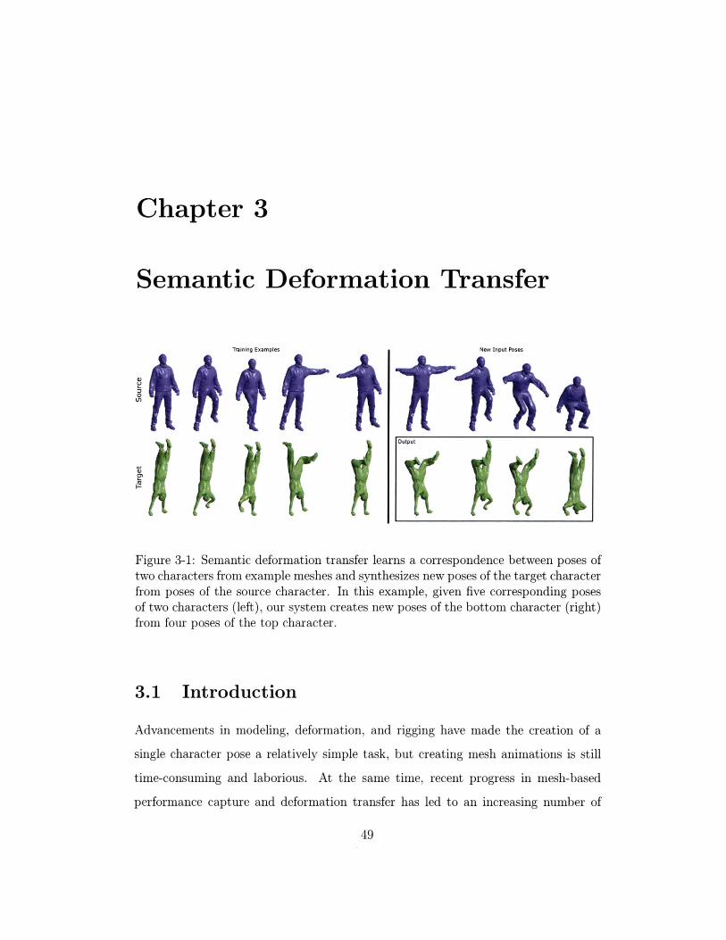
Figure 3-1: Semantic deformation transfer learns a correspondence between poses oftwo characters from example meshes and synthesizes new poses of the target characterfrom poses of the source character. In this example, given five corresponding posesof two characters (left), our system creates new poses of the bottom character (right)from four poses of the top character.
3.1 Introduction
Advancements in modeling, deformation, and rigging have made the creation of a
single character pose a relatively simple task, but creating mesh animations is still
time-consuming and laborious. At the same time, recent progress in mesh-based
performance capture and deformation transfer has led to an increasing number of
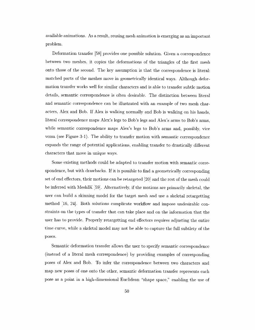
available animations. As a result, reusing mesh animation is emerging as an important
problem.
Deformation transfer [58] provides one possible solution. Given a correspondence
between two meshes, it copies the deformations of the triangles of the first mesh
onto those of the second. The key assumption is that the correspondence is literal:
matched parts of the meshes move in geometrically identical ways. Although defor-
mation transfer works well for similar characters and is able to transfer subtle motion
details, semantic correspondence is often desirable. The distinction between literal
and semantic correspondence can be illustrated with an example of two mesh char-
acters, Alex and Bob. If Alex is walking normally and Bob is walking on his hands,
literal correspondence maps Alex's legs to Bob's legs and Alex's arms to Bob's arms,
while semantic correspondence maps Alex's legs to Bob's arms and, possibly, vice
versa (see Figure 3-1). The ability to transfer motion with semantic correspondence
expands the range of potential applications, enabling transfer to drastically different
characters that move in unique ways.
Some existing methods could be adapted to transfer motion with semantic corre-
spondence, but with drawbacks. If it is possible to find a geometrically corresponding
set of end effectors, their motions can be retargeted [20] and the rest of the mesh could
be inferred with MeshIK [59]. Alternatively, if the motions are primarily skeletal, the
user can build a skinning model for the target mesh and use a skeletal retargetting
method [16, 24]. Both solutions complicate workflow and impose undesirable con-
straints on the types of transfer that can take place and on the information that the
user has to provide. Properly retargetting end effectors requires adjusting the entire
time curve, while a skeletal model may not be able to capture the full subtlety of the
poses.
Semantic deformation transfer allows the user to specify semantic correspondence
(instead of a literal mesh correspondence) by providing examples of corresponding
poses of Alex and Bob. To infer the correspondence between two characters and
map new poses of one onto the other, semantic deformation transfer represents each
pose as a point in a high-dimensional Euclidean "shape space," enabling the use of
Source shape space
I f Project InputposeSource examples
Weights: (0.7, 0.3)
Interpolate
COg CVgI
Target examples Target shape space Output pose
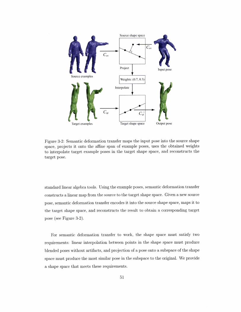
Figure 3-2: Semantic deformation transfer maps the input pose into the source shapespace, projects it onto the affine span of example poses, uses the obtained weightsto interpolate target example poses in the target shape space, and reconstructs thetarget pose.
standard linear algebra tools. Using the example poses, semantic deformation transfer
constructs a linear map from the source to the target shape space. Given a new source
pose, semantic deformation transfer encodes it into the source shape space, maps it to
the target shape space, and reconstructs the result to obtain a corresponding target
pose (see Figure 3-2).
For semantic deformation transfer to work, the shape space must satisfy two
requirements: linear interpolation between points in the shape space must produce
blended poses without artifacts, and projection of a pose onto a subspace of the shape
space must produce the most similar pose in the subspace to the original. We provide
a shape space that meets these requirements.
.. ....... . . ....... . ... ..... ....
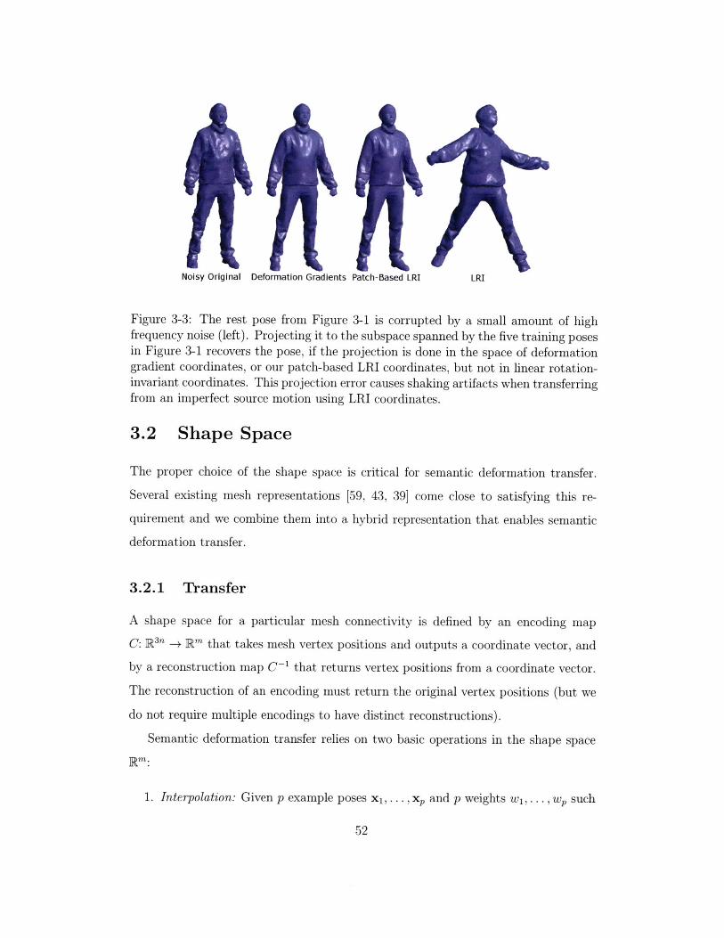
Noisy Original Deformation Gradients Patch-Based LRI LRI
Figure 3-3: The rest pose from Figure 3-1 is corrupted by a small amount of highfrequency noise (left). Projecting it to the subspace spanned by the five training posesin Figure 3-1 recovers the pose, if the projection is done in the space of deformationgradient coordinates, or our patch-based LRI coordinates, but not in linear rotation-invariant coordinates. This projection error causes shaking artifacts when transferringfrom an imperfect source motion using LRI coordinates.
3.2 Shape Space
The proper choice of the shape space is critical for semantic deformation transfer.
Several existing mesh representations [59, 43, 39] come close to satisfying this re-
quirement and we combine them into a hybrid representation that enables semantic
deformation transfer.
3.2.1 Transfer
A shape space for a particular mesh connectivity is defined by an encoding map
C: R3, -+ R' that takes mesh vertex positions and outputs a coordinate vector, and
by a reconstruction map C- 1 that returns vertex positions from a coordinate vector.
The reconstruction of an encoding must return the original vertex positions (but we
do not require multiple encodings to have distinct reconstructions).
Semantic deformation transfer relies on two basic operations in the shape space
R":
1. Interpolation: Given p example poses x 1, . .. , x, and p weights w1, . . . , w, such
that E> wi = 1, compute T1 wixi, the affine combination of the poses.
2. Projection: Given p example poses x 1,. . . , x, and another pose q, compute p
weights wi, . . . , w, that minimize
P
q - Wixi subject to wi = 1.i=1
Letting the cross denote the pseudoinverse, the solution is:
W2 [[X2 -X 1 X3 -X 1 ... xpx]t[q - xi],
and wi = 1 - E= wi.
We focus on affine rather than linear interpolation and projection because the origin
of the shape space has no special meaning for the transfer.
A shape space is suitable for interpolation if affine combinations of several poses
do not result in shrinking or other artifacts (at least when the coefficients are not too
negative). Suitability for projection means that the projection of a pose onto an affine
span of other poses must retain the characteristics of the unprojected pose as much
as possible. For example, random high-frequency noise must be nearly orthogonal to
meaningful pose changes (see Figure 3-3) and deformations in different parts of the
mesh should be nearly orthogonal to each other (see Figure 3-5).
A shape space that supports interpolation and projection enables semantic defor-
mation transfer with the following simple algorithm (Figure 3-2):
1. Given p pairs of example poses, encode them into the source and target shape
spaces using Csrc and Ctgt. Precompute the pseudoinverse (using singular value
decomposition) for projection in the source space.
2. Given a new source pose, encode it into the source shape space and use pro-
jection to express it as an affine combination of the source example poses with
weights wi, ... , wp .
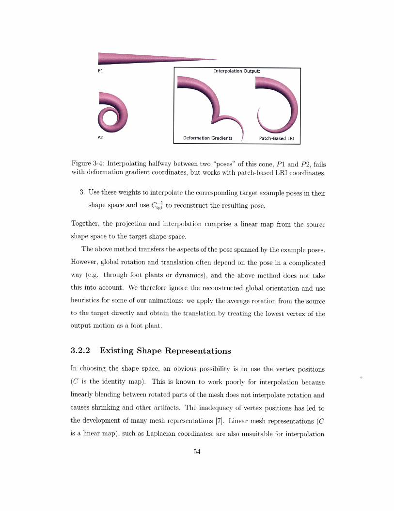
P1 Interpolation Output:
P2 Deformation Gradients Patch-Based LRI
Figure 3-4: Interpolating halfway between two "poses" of this cone, P1 and P2, failswith deformation gradient coordinates, but works with patch-based LRI coordinates.
3. Use these weights to interpolate the corresponding target example poses in their
shape space and use Cj to reconstruct the resulting pose.
Together, the projection and interpolation comprise a linear map from the source
shape space to the target shape space.
The above method transfers the aspects of the pose spanned by the example poses.
However, global rotation and translation often depend on the pose in a complicated
way (e.g. through foot plants or dynamics), and the above method does not take
this into account. We therefore ignore the reconstructed global orientation and use
heuristics for some of our animations: we apply the average rotation from the source
to the target directly and obtain the translation by treating the lowest vertex of the
output motion as a foot plant.
3.2.2 Existing Shape Representations
In choosing the shape space, an obvious possibility is to use the vertex positions
(C is the identity map). This is known to work poorly for interpolation because
linearly blending between rotated parts of the mesh does not interpolate rotation and
causes shrinking and other artifacts. The inadequacy of vertex positions has led to
the development of many mesh representations [7]. Linear mesh representations (C
is a linear map), such as Laplacian coordinates, are also unsuitable for interpolation
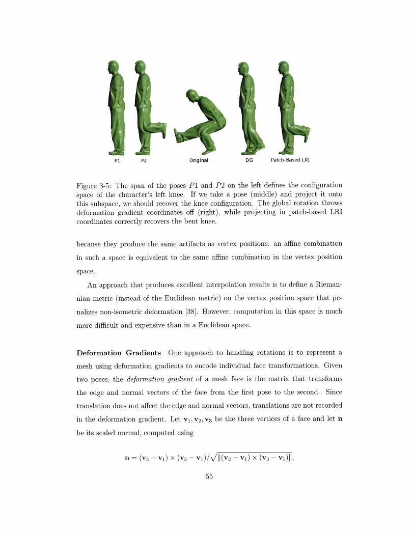
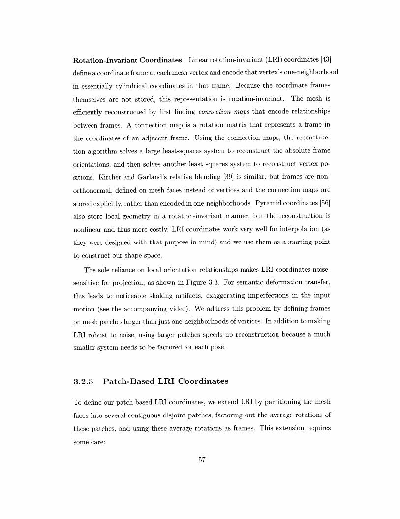
P1 P2 Original DG Patch-Based LRI
Figure 3-5: The span of the poses P1 and P2 on the left defines the configurationspace of the character's left knee. If we take a pose (middle) and project it ontothis subspace, we should recover the knee configuration. The global rotation throwsdeformation gradient coordinates off (right), while projecting in patch-based LRIcoordinates correctly recovers the bent knee.
because they produce the same artifacts as vertex positions: an affine combination
in such a space is equivalent to the same affine combination in the vertex position
space.
An approach that produces excellent interpolation results is to define a Rieman-
nian metric (instead of the Euclidean metric) on the vertex position space that pe-
nalizes non-isometric deformation [381. However, computation in this space is much
more difficult and expensive than in a Euclidean space.
Deformation Gradients One approach to handling rotations is to represent a
mesh using deformation gradients to encode individual face transformations. Given
two poses, the deformation gradient of a mesh face is the matrix that transforms
the edge and normal vectors of the face from the first pose to the second. Since
translation does not affect the edge and normal vectors, translations are not recorded
in the deformation gradient. Let v1, v 2 , v3 be the three vertices of a face and let n
be its scaled normal, computed using
n= (v 2 - v1) x (v 3 - v1)/ /||(v2 - vi) x (v3 - vi)I,
following Sumner and Popovid [58). Let 91, i' 2 , v 3 , and i be the corresponding
vertices and scaled normal in the rest pose. The deformation gradient is the following
3 x 3 matrix:
D = [v2 - vi v 3 - v i n][V2 -V 1 9 3l - 1 n]-- -.
A mesh can be represented by recording the deformation gradients of all of the
faces relative to a rest pose. For example, MeshIK uses such a representation for
projection [59]. However, linearly interpolating deformation gradients does not pre-
serve rotations. Therefore, for interpolation, MeshIK performs a polar decomposition
of each deformation gradient QS = D and stores S and log Q separately, allowing
rotations to be interpolated in logarithmic space.
This representation becomes problematic when the mesh undergoes a large global
rotation relative to the rest pose (imagine interpolating the rest pose and a perturbed
rest pose rotated 180 degrees: each face rotation would choose a different interpolation
path, depending on its perturbation). Factoring out the average deformation gradient
rotation (found by using polar decomposition to project Efefaces Q/ to a rotation
matrix) and storing it separately avoids this problem. We refer to this representation
as deformation gradient coordinates.
Even with the global rotation factored out, this representation has two more
drawbacks. For interpolation, factoring out the average rotation may not be enough
and interpolating between two poses in which some faces have rotated more than 180
degrees will result in discontinuity artifacts (Figure 3-4). These types of artifacts can
often arise in deformations of tails, snakes, and tentacles, for example. For projection,
the deformation gradient coordinates are not locally rotation invariant, resulting in
dependency between degrees of freedom that should be independent. Figure 3-5
shows an experiment in which we project a pose with a bent back and a bent knee
onto the subspace of poses spanning possible knee configurations. In deformation
gradient coordinates, the dependence between the bent back and bent knee results in
an incorrect projection.
Rotation-Invariant Coordinates Linear rotation-invariant (LRI) coordinates [43]
define a coordinate frame at each mesh vertex and encode that vertex's one-neighborhood
in essentially cylindrical coordinates in that frame. Because the coordinate frames
themselves are not stored, this representation is rotation-invariant. The mesh is
efficiently reconstructed by first finding connection maps that encode relationships
between frames. A connection map is a rotation matrix that represents a frame in
the coordinates of an adjacent frame. Using the connection maps, the reconstruc-
tion algorithm solves a large least-squares system to reconstruct the absolute frame
orientations, and then solves another least squares system to reconstruct vertex po-
sitions. Kircher and Garland's relative blending [39] is similar, but frames are non-
orthonormal, defined on mesh faces instead of vertices and the connection maps are
stored explicitly, rather than encoded in one-neighborhoods. Pyramid coordinates [56]
also store local geometry in a rotation-invariant manner, but the reconstruction is
nonlinear and thus more costly. LRI coordinates work very well for interpolation (as
they were designed with that purpose in mind) and we use them as a starting point
to construct our shape space.
The sole reliance on local orientation relationships makes LRI coordinates noise-
sensitive for projection, as shown in Figure 3-3. For semantic deformation transfer,
this leads to noticeable shaking artifacts, exaggerating imperfections in the input
motion (see the accompanying video). We address this problem by defining frames
on mesh patches larger than just one-neighborhoods of vertices. In addition to making
LRI robust to noise, using larger patches speeds up reconstruction because a much
smaller system needs to be factored for each pose.
3.2.3 Patch-Based LRI Coordinates
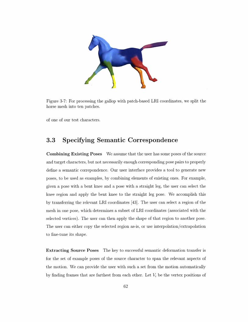
To define our patch-based LRI coordinates, we extend LRI by partitioning the mesh
faces into several contiguous disjoint patches, factoring out the average rotations of
these patches, and using these average rotations as frames. This extension requires
some care:
" Extending cylindrical coordinates to larger patches directly does not work be-
cause deformations of larger patches are likely to have faces that rotate relative
to the patch frame. As with Cartesian coordinates, linearly interpolating be-
tween rotated triangles in cylindrical coordinates does not (in general) interpo-
late the rotation. We therefore encode the local geometry of the larger patches
using polar decompositions of deformation gradients.
" LRI reconstructs connection maps between frames from overlapping vertex
neighborhoods. Using overlapping patches would make reconstruction more
expensive: to solve for the patch frames, we would first need to reconstruct
the individual patches from local deformation gradients and then reconstruct
the entire model from deformation gradients again (so as not to have seams).
Instead, like Kircher and Garland [391, we store the connection maps explicitly,
but unlike them, we use orthonormal frames because this avoids global shear
artifacts in reconstruction that our experiments revealed (see video).
" We encode rotations with matrix logarithms. Compared to the nonlinear quater-
nion interpolation, linearly blending matrix logarithms is not rotation-invariant
and introduces error. Because this interpolation error is smallest when rotations
are small or coaxial, we use deformation gradients relative to a rest pose. For
the same reason, unlike LRI, we work with patch frames relative to the rest
pose. As a result, when we encode the rest pose, all of our connection maps are
the identity. Our experiments confirmed that the results are not sensitive to
the choice of the rest pose, as long as it is a reasonable pose for the character.
Encoding Let Df be the deformation gradient of mesh face f relative to the rest
pose and let QjSj = Df be the polar decomposition of this deformation gradient.
Let Q be the average of all Qf's (computed by orthonormalizing Ef Qf using polar
decomposition). Let P1 , . . ., Pk be the patches and let p(f) be the index of the patch
to which face f belongs. Let G 1 , ... , Gk be the average rotations of the deformation
Restpose
Currentpose
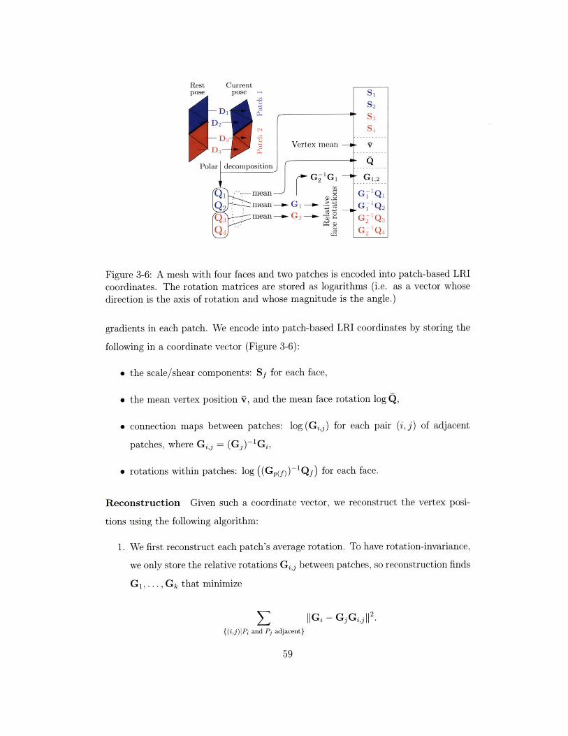
Figure 3-6: A mesh with four faces and two patches is encoded into patch-based LRIcoordinates. The rotation matrices are stored as logarithms (i.e. as a vector whosedirection is the axis of rotation and whose magnitude is the angle.)
gradients in each patch. We encode into patch-based LRI coordinates by storing the
following in a coordinate vector (Figure 3-6):
" the scale/shear components: Sf for each face,
* the mean vertex position V, and the mean face rotation log Q,
" connection maps between patches: log (Gij) for each pair (i, j) of adjacent
patches, where Gij = (Gj)-'Gi,
" rotations within patches: log ((G,(f)) 1 Qf) for each face.
Reconstruction Given such a coordinate vector, we reconstruct the vertex posi-
tions using the following algorithm:
1. We first reconstruct each patch's average rotation. To have rotation-invariance,
we only store the relative rotations Gij between patches, so reconstruction finds
the source mesh in i = 1 ... p example poses. We start with a rest pose V1. We set
V2 to be the frame of the motion farthest from V1, and in general Vi to be the frame
farthest from the subspace spanned by Vi through Vi. All distances are measured in
the shape space of patch-based LRI coordinates. This leaves it to the user to specify
only the target's corresponding poses.
Splitting Independent Parts In many cases, the user can reduce the amount
of work to construct example poses by decomposing a semantic correspondence into
correspondences between independent parts of the meshes. For example, for trans-
fering Alex's normal walk to Bob's walk on his hands, the mapping of Alex's upper
body to Bob's lower body can be specified independently from the mapping of Alex's
lower body to Bob's upper body. When the user specifies such a decomposition on
Alex, our prototype UI extracts Alex's upper body motion separately from his lower
body motion (using LRI coordinates from the rest pose to keep the remainder of Alex
fixed). It then uses the procedure in the previous paragraph to extract representative
poses from both the upper body and the lower body motions. The result is that half
of the poses need only the upper body posed and half of the poses only need the lower
body posed.
3.4 Results
We applied our method to publicly available mesh animations from performance cap-
ture [66] and deformation transfer [58]. The motions we created (available in the
accompanying video) are listed in Table 3.1.
Although we did not spend much time optimizing our implementation, it is quite
fast. The flamingo is the largest mesh we tested at 52,895 triangles. Encoding
a frame of the flamingo into patch-based LRI coordinates takes 0.22 seconds and
reconstruction takes 0.25 seconds on a 1.73 Ghz Core Duo laptop. Given the example
poses, applying semantic deformation transfer to the 175 frame crane animation takes
136 seconds, including reading the data from disk, partitioning both meshes into
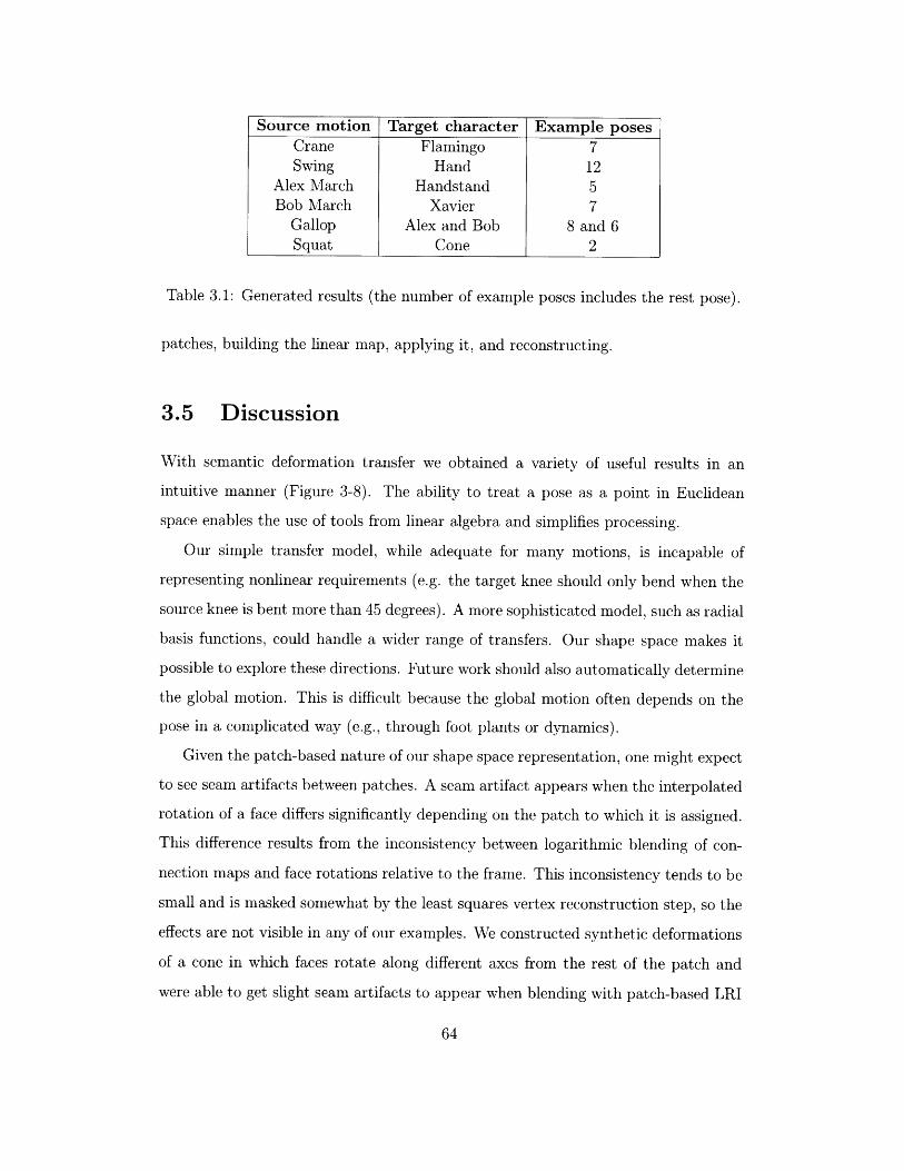
Table 3.1: Generated results (the number of example poses includes the rest pose).
patches, building the linear map, applying it, and reconstructing.
3.5 Discussion
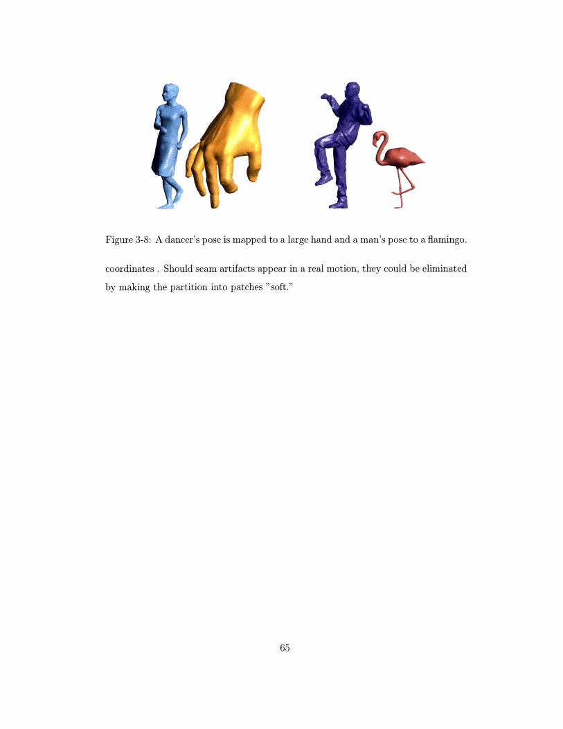
With semantic deformation transfer we obtained a variety of useful results in an
intuitive manner (Figure 3-8). The ability to treat a pose as a point in Euclidean
space enables the use of tools from linear algebra and simplifies processing.
Our simple transfer model, while adequate for many motions, is incapable of
representing nonlinear requirements (e.g. the target knee should only bend when the
source knee is bent more than 45 degrees). A more sophisticated model, such as radial
basis functions, could handle a wider range of transfers. Our shape space makes it
possible to explore these directions. Future work should also automatically determine
the global motion. This is difficult because the global motion often depends on the
pose in a complicated way (e.g., through foot plants or dynamics).
Given the patch-based nature of our shape space representation, one might expect
to see seam artifacts between patches. A seam artifact appears when the interpolated
rotation of a face differs significantly depending on the patch to which it is assigned.
This difference results from the inconsistency between logarithmic blending of con-
nection maps and face rotations relative to the frame. This inconsistency tends to be
small and is masked somewhat by the least squares vertex reconstruction step, so the
effects are not visible in any of our examples. We constructed synthetic deformations
of a cone in which faces rotate along different axes from the rest of the patch and
were able to get slight seam artifacts to appear when blending with patch-based LRI
Source motion Target character Example posesCrane Flamingo 7Swing Hand 12
Alex March Handstand 5Bob March Xavier 7
Gallop Alex and Bob 8 and 6Squat Cone 2
Figure 3-8: A dancer's pose is mapped to a large hand and a man's pose to a flamingo.
coordinates . Should seam artifacts appear in a real motion, they could be eliminated
by making the partition into patches "soft."
..... .............................
66
Chapter 4
Conclusion
We presented two methods that assist an artist trying to create character animation.
The first method is for automatically rigging an unfamiliar character for skeletal
animation. In conjunction with existing techniques, it allows a user to go from a static
mesh to an animated character quickly and effortlessly. We have shown that using
this method, Pinocchio can animate a wide range of characters. We also believe that
some of our techniques, such as finding LBS weights or using examples to learn the
weights of a linear combination of penalty functions, can be useful in other contexts.
The paper describing the automatic rigging method was published in 2007 [3] and
the source to Pinocchio released under a permissive license. Since then, our method
for finding LBS weights has been implemented in the free modeling package Blender
(under the name "Bone Heat") and plugins are available for Maya. The response from
artists has been very positive: claims of enhanced productivity abound. A prototype
game, called Phorm, based on Pinocchio has also been developed by GAMBIT, the
Singapore-MIT game lab. It uses Pinocchio to enable the player to modify his or her
character's geometry as part of the gameplay.
Since the original publication, several methods have also proposed alternatives or
improvements to our method. To improve LBS weights, a method has been proposed
called "Bone Glow" [70]. Bone glow appears to produce better results in some cases,
although the paper does not discuss performance. To avoid LBS artifacts and to have
more control over the deformation, another recent method almost-automatically con-
structs a cage, based on templates of joint behaviors [34]. The key advantage of both
this method and Pinocchio is that the user can specify at once how an entire class of
characters is rigged (either with the cage templates, or with the template skeleton).For skeleton embedding, a method based on generalizing Centroidal Voronoi Tessel-
lation has been proposed that makes fewer assumptions about the character than our
method [45].
Semantic deformation transfer has been published more recently and we do not
yet have the benefit of hindsight. However, some possibilities for further work in this
direction are intriguing. Although projection in our shape space produces intuitive
results, we do not know whether distance in the shape space is a good measure of
pose dissimilarity, or, indeed how to measure pose dissimilarity at all. Formulating
such a metric would enable a quantitative comparison of different shape spaces and
provide a principled way of choosing weights for our coordinates.
Determining the minimum amount of information necessary to specify a transfer
is an interesting conceptual and practical challenge: while a surface correspondence
enables literal deformation transfer and a few example poses enable semantic de-
formation transfer, can we perform semantic motion transfer using example motion
clips? Different characters move with different rhythms in a way that is difficult to
capture with just a mapping between their pose spaces. Building a model that takes
time or even physics into account could lead to much higher quality automatically
generated animations than what is currently possible.
4.1 Simplifying 3D Content Creation
In this work, we presented two specific tools that can reduce the effort required of
artists and animators. The question of how to streamline the 3D content creation
process in general remains. To date, production studios have sidestepped this problem
by hiring more artists. Nonetheless, in principle, it should be possible for a single
person to play the part of the "director," specifying artistic style, characters, setting,
and story, and have the work of the rest of the team done by intelligent software. This
is, of course, currently science fiction: I believe we are still at a point when relatively
small improvements in tools can have a very large effect on productivity.
There are two obvious directions for improvement: developing new underlying
technology that is more flexible and intuitive and improving the user interface. This
thesis has almost exclusively focused on the first direction, but without a good inter-
face, technology improvements are useless. In terms of user interfaces, there is a very
large gulf between UI research prototypes and production systems.
On the research end, as is inevitable given the limited resources, prototypes are
generally quite primitive. While illustrating the authors' idea, these prototypes do not
address the scalability concern-whether the idea can function inside a production
system. In much otherwise good research (e.g., the Teddy-Fibermesh line of work),
the answer seems to be "no."
On the production end, developers have noticed that professional artists are very
good at adapting and working around limitations in software, as long as there is a
path to their desired end result. This has led to software whose UIs are far more
complicated than necessary, requiring many steps for seemingly simple tasks. I have
witnessed a professional 3D modeler who was very fast and proficient in Maya spend
an hour on a part that could have been modeled in twenty minutes using a recently
published system [53].
The unfortunate result of this distance between research and production is that
progress has been slow: most modelers, riggers, and animators today don't work much
differently than they did ten years ago. Researchers often don't have the capability
to evaluate their ideas on a large scale, while deficiencies in production Uls greatly
obscure the underlying technical issues that need to be addressed to improve produc-
tivity. A clean, extendible, stable toolchain with a well-thought-out UI (as Eclipse is
to Java programming, for example) could break the impasse and make life easier for
artists (at least those remaining employed) while facilitating research. Building such
a system is a very difficult undertaking and given the entrenched market position of
existing software, not many entities could attempt it. However, without it, progress
will continue to be slow.
70
Appendix A
Penalty Functions for Automatic
Rigging
A.1 Skeleton Joint Attributes
The skeleton joints can be supplied with the following attributes to improve quality
and performance (without sacrificing too much generality):
" A joint may be marked symmetric with respect to another joint. This results
in symmetry penalties if the distance between the joint and its parent differs
from the distance between the symmetric joint and its parent.
" A joint may be marked as a foot. This results in a penalty if the joint is not in
the bottommost position.
* A joint may be marked as "fat." This restricts the possible placement of the
joint to the center of the o- largest spheres. We use o = 50. In our biped
skeleton, hips, shoulders and the head are marked as "fat."
A.2 Discrete Penalty Basis Functions
The discrete penalty function measures the quality of a reduced skeleton embedding
into the discretized character volume. It is a linear combination of basis penalty
functions (Pinocchio uses nine). The weights were determined automatically by the
maximum-margin method described in the paper and are (0.27, 0.23, 0.07, 0.46, 0.14,
0.12, 0.72, 0.05, 0.33) in the order that the penalties are presented.
The specific basis penalty functions were constructed in an ad hoc manner. They
are summed over all embedded bones (or joints), as applicable. Slight changes in the
specific constants used should not have a significant effect on results. We use the
notation sgi (x) to denote the bounded linear interpolation function that is equal to
b if x < a, d if x > c, and b + (d - b)(x - a)/(c - a) otherwise.
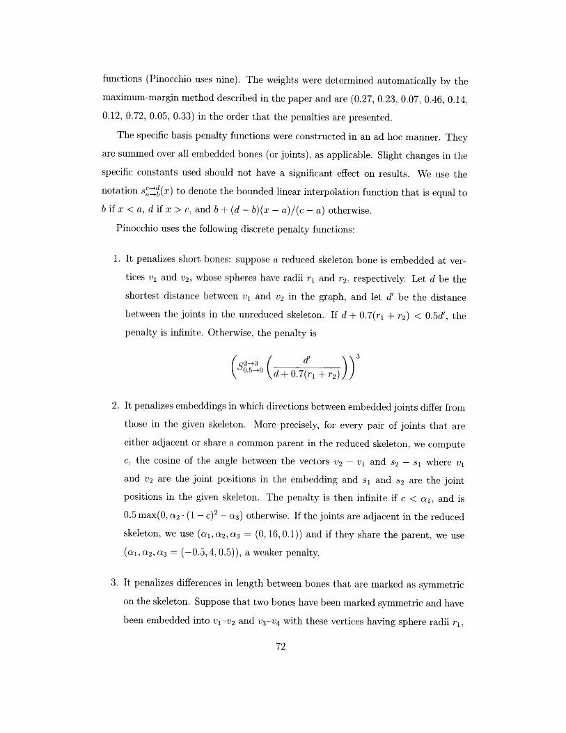
Pinocchio uses the following discrete penalty functions:
1. It penalizes short bones: suppose a reduced skeleton bone is embedded at ver-
tices vi and v2 , whose spheres have radii r1 and r2, respectively. Let d be the
shortest distance between vi and v2 in the graph, and let d' be the distance
between the joints in the unreduced skeleton. If d + 0.7(r1 + r2 ) < 0.5d', the
penalty is infinite. Otherwise, the penalty is
S2-3 d' 3
.5-0 ( + 0.7 r1+ r2)))
2. It penalizes embeddings in which directions between embedded joints differ from
those in the given skeleton. More precisely, for every pair of joints that are
either adjacent or share a common parent in the reduced skeleton, we compute
c, the cosine of the angle between the vectors v2 - vi and s 2 - s1 where vi
and v2 are the joint positions in the embedding and si and S2 are the joint
positions in the given skeleton. The penalty is then infinite if c < ai, and is
0.5 max(0, a 2 . (1 - c)2 - a 3 ) otherwise. If the joints are adjacent in the reduced
skeleton, we use (ai, a 2 , a3 = (0, 16, 0.1)) and if they share the parent, we use
(ai, a 2, a3 = (-0.5, 4, 0.5)), a weaker penalty.
3. It penalizes differences in length between bones that are marked as symmetric
on the skeleton. Suppose that two bones have been marked symmetric and have
been embedded into v1 -v 2 and v3-v 4 with these vertices having sphere radii r1 ,
r2 , r3 , and r4, respectively. Suppose that the distance along the graph edges
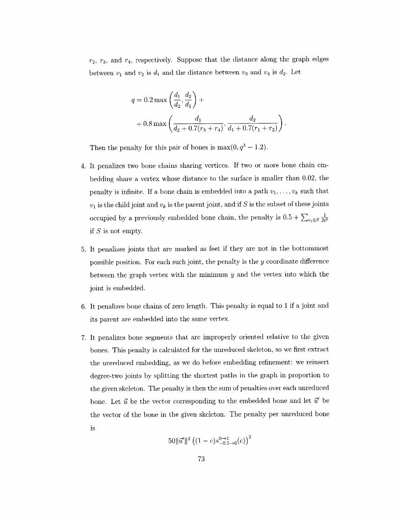
between vi and v2 is di and the distance between v3 and v4 is d2. Let
0 (d 1 d2
q = 0.2 max ,iId +m d2 d1 )
+ 0.8 maxd2 + 0.7(r 3 + r4 )' di + 0.7(r 1 + r2)
Then the penalty for this pair of bones is max(0, q3 - 1.2).
4. It penalizes two bone chains sharing vertices. If two or more bone chain em-
bedding share a vertex whose distance to the surface is smaller than 0.02, the
penalty is infinite. If a bone chain is embedded into a path V1, . . ., Vk such that
vi is the child joint and ok is the parent joint, and if S is the subset of these joints1
occupied by a previously embedded bone chain, the penalty is 0.5 + EviES 2i2
if S is not empty.
5. It penalizes joints that are marked as feet if they are not in the bottommost
possible position. For each such joint, the penalty is the y coordinate difference
between the graph vertex with the minimum y and the vertex into which the
joint is embedded.
6. It penalizes bone chains of zero length. This penalty is equal to 1 if a joint and
its parent are embedded into the same vertex.
7. It penalizes bone segments that are improperly oriented relative to the given
bones. This penalty is calculated for the unreduced skeleton, so we first extract
the unreduced embedding, as we do before embedding refinement: we reinsert
degree-two joints by splitting the shortest paths in the graph in proportion to
the given skeleton. The penalty is then the sum of penalties over each unreduced
bone. Let U' be the vector corresponding to the embedded bone and let i' be
the vector of the bone in the given skeleton. The penalty per unreduced bone
is
50|11'|| 2 ((1 - c)sO0_,(c))2
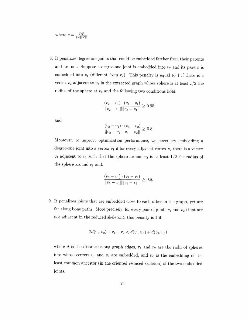
where c - , .__
8. It penalizes degree-one joints that could be embedded farther from their parents
and are not. Suppose a degree-one joint is embedded into v2 and its parent is
embedded into vi (different from v2 ). This penalty is equal to 1 if there is a
vertex v3 adjacent to v2 in the extracted graph whose sphere is at least 1/2 the
radius of the sphere at v2 and the following two conditions hold:
(v 2 - vI) - (v3 - v1 ) > 0.95||V2 V 1|| -V3 1 || -
and
(v 2 - v1) - (v 3 - v 2) > 0.8.11v2 v1||||v3 V2| ~
Moreover, to improve optimization performance, we never try embedding a
degree-one joint into a vertex vi if for every adjacent vertex v2 there is a vertex
v3 adjacent to vi such that the sphere around v3 is at least 1/2 the radius of
the sphere around vi and:
(v 3 - vi) - (v1 - v 2 ) > 0.8.||V3- v1||||v1 - V211
9. It penalizes joints that are embedded close to each other in the graph, yet are
far along bone paths. More precisely, for every pair of joints vi and v2 (that are
not adjacent in the reduced skeleton), this penalty is 1 if
2d(v1,v 2) + r1 + r2 < d(v1,VL) + d(v 2 , VL)
where d is the distance along graph edges, r1 and r 2 are the radii of spheres
into whose centers vi and v2 are embedded, and VL is the embedding of the
least common ancestor (in the oriented reduced skeleton) of the two embedded
joints.
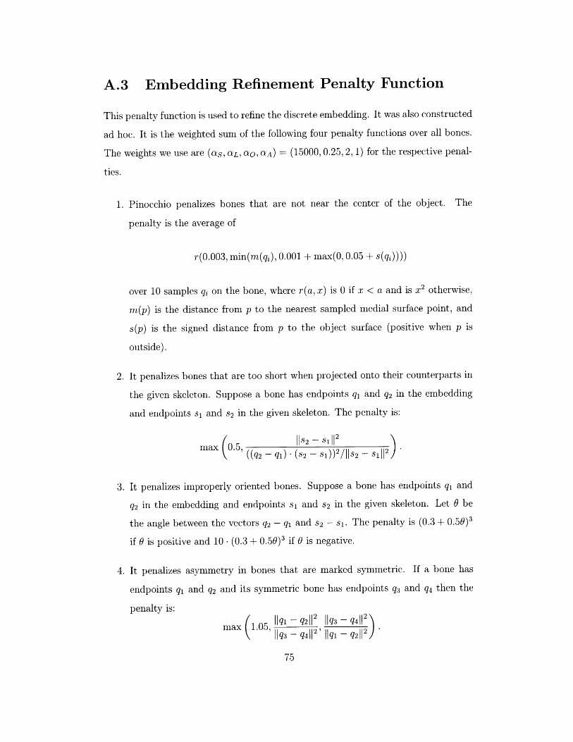
A.3 Embedding Refinement Penalty Function
This penalty function is used to refine the discrete embedding. It was also constructed
ad hoc. It is the weighted sum of the following four penalty functions over all bones.
The weights we use are (as, aL, a0, aA) = (15000, 0.25, 2, 1) for the respective penal-
ties.
1. Pinocchio penalizes bones that are not near the center of the object. The
This penalty appears in the sum once for every pair of symmetric bones.
Bibliography
[1] David Anderson, James L. Frankel, Joe Marks, Aseem Agarwala, Paul Beardsley,Jessica Hodgins, Darren Leigh, Kathy Ryall, Eddie Sullivan, and Jonathan S.Yedidia. Tangible interaction + graphical interpretation: a new approach to 3dmodeling. In Proceedings of ACM SIGGRAPH 2000, Annual Conference Series,pages 393-402, July 2000.
[2] Okan Arikan, David A. Forsyth, and James F. O'Brien. Motion synthesis from
annotations. ACM Transactions on Graphics, 22(3):402-408, July 2003.
[3] Ilya Baran and Jovan Popovid. Automatic rigging and animation of 3d characters.ACM Transactions on Graphics, 26(3), 2007. In press.
[4] Ilya Baran and Jovan Popovid. Pinocchio results video.http://people.csail.mit.edu/ibaran/pinocchio.avi, 2007.
[5] Jules Bloomenthal and Chek Lim. Skeletal methods of shape manipulation. InProceedings of the International Conference on Shape Modeling and Applications,page 44, 1999.
[6] Gunilla Borgefors, Ingela Nystrm, and Gabriella Sanniti Di Baja. Computingskeletons in three dimensions. Pattern Recognition, 32(7):1225 - 1236, 1999.
[7] Mario Botsch and Olga Sorkine. On linear variational surface deformation meth-
ods. IEEE Transactions on Visualization and Computer Graphics, 14(1):213-230, 2008.
[8] Matthew Brand and Aaron Hertzmann. Style machines. In Proceedings of ACMSIGGRAPH 2000, Computer Graphics Proceedings, Annual Conference Series,pages 183-192, July 2000.
[9] C.J.C. Burges. A Tutorial on Support Vector Machines for Pattern Recognition.Data Mining and Knowledge Discovery, 2(2):121-167, 1998.
[10] Steve Capell, Seth Green, Brian Curless, Tom Duchamp, and Zoran Popovi6. In-
teractive skeleton-driven dynamic deformation. A CM Transactions on Graphics,21(3):586-593, August 2002.
[11] Kwang-Jin Choi and Hyeong-Seok Ko. Online motion retargetting. Journal of
Visualization and Computer Animation, 11(5):223-235, December 2000.
[12] Nicu D. Cornea, Deborah Silver, and Patrick Min. Curve-skeleton properties,applications, and algorithms. IEEE Transactions on Visualization and ComputerGraphics, 13(3):530-548, 2007.
[13] Marco da Silva, Yeuhi Abe, and Jovan Popovid. Interactive simulation of stylizedhuman locomotion. ACM Transactions on Graphics, 27(3):82:1-82:10, August2008.
[14] Edilson de Aguiar, Carsten Stoll, Christian Theobalt, Naveed Ahmed, Hans-Peter Seidel, and Sebastian Thrun. Performance capture from sparse multi-viewvideo. ACM Transactions on Graphics, 27(3):98:1-98:10, August 2008.
[15] Edilson de Aguiar, Christian Theobalt, Marcus Magnor, and Hans-Peter Seidel.Reconstructing human shape and motion from multi-view video. In Conferenceon Visual Media Production, pages 44-51, December 2005.
[16] Mira Dontcheva, Gary Yngve, and Zoran Popovid. Layered acting for characteranimation. ACM Transactions on Graphics, 22(3):409-416, July 2003.
[17] Michael S. Floater. Mean value coordinates. Computer Aided Geometric Design,20(1):19-27, March 2003.
[18] Sarah F. Frisken, Ronald N. Perry, Alyn P. Rockwood, and Thouis R. Jones.Adaptively sampled distance fields: A general representation of shape for com-puter graphics. In Proceedings of ACM SIGGRAPH 2000, Annual ConferenceSeries, pages 249-254, July 2000.
[19] Philip E. Gill, Walter Murray, and Margaret H. Wright. Practical Optimization.Academic Press, London, 1989.
[20] Michael Gleicher. Retargetting motion to new characters. In Proceedings of SIG-GRAPH 98, Computer Graphics Proceedings, Annual Conference Series, pages33-42, July 1998.
[21] Michael Gleicher. Comparing constraint-based motion editing methods. Graph-ical Models, 63(2):107-134, March 2001.
[22] Steven Gold and Anand Rangarajan. A graduated assignment algorithm forgraph matching. IEEE Transactions on Pattern Analysis and Machine Intelli-gence, 18(4):377-388, 1996.
[23] Radek Grzeszczuk, Demetri Terzopoulos, and Geoffrey Hinton. Neuroanimator:Fast neural network emulation and control of physics-based models. In Proceed-ings of SIGGRAPH 98, Computer Graphics Proceedings, Annual ConferenceSeries, pages 9-20, July 1998.
[24] Eugene Hsu, Sommer Gentry, and Jovan Popovid. Example-based control of hu-man motion. In 2004 A CM SIGGRAPH / Eurographics Symposium on ComputerAnimation, pages 69-77, July 2004.
[25] Eugene Hsu, Kari Pulli, and Jovan Popovid. Style translation for human motion.ACM Transactions on Graphics, 24(3):1082-1089, August 2005.
[26] Takeo Igarashi and John F. Hughes. Smooth meshes for sketch-based freeformmodeling. In 2003 ACM Symposium on Interactive 3D Graphics, pages 139-142,April 2003.
[27] Takeo Igarashi, Satoshi Matsuoka, and Hidehiko Tanaka. Teddy: A sketching in-terface for 3d freeform design. In Proceedings of ACM SIGGRAPH 1999, AnnualConference Series, pages 409-416, July 1999.
[28] Takeo Igarashi, Tomer Moscovich, and John F. Hughes. As-rigid-as-possibleshape manipulation. ACM Transactions on Graphics, 24(3):1134-1141, August2005.
[29] Takeo Igarashi, Tomer Moscovich, and John F. Hughes. Spatial keyframing forperformance-driven animation. In Symposium on Computer Animation (SCA),pages 107-115, jul 2005.
[30] Doug L. James and Christopher D. Twigg. Skinning mesh animations. ACMTransactions on Graphics, 24(3):399-407, August 2005.
[31] Jerzy W. Jaromczyk and Godfried T. Toussaint. Relative neighborhood graphsand their relatives. Proceedings of IEEE, 80(9):1502-1517, September 1992.
[32] Pushkar Joshi, Mark Meyer, Tony DeRose, Brian Green, and Tom Sanocki. Har-monic coordinates for character articulation. ACM Transactions on Graphics,26(3):71:1-71:9, July 2007.
[33] Tao Ju, Scott Schaefer, and Joe Warren. Mean value coordinates for closedtriangular meshes. A CM Transactions on Graphics, 24(3):561-566, August 2005.
[34] Tao Ju, Qian-Yi Zhou, Michiel van de Panne, Daniel Cohen-Or, and UlrichNeumann. Reusable skinning templates using cage-based deformations. ACMTransactions on Graphics, 27(5):122:1-122:10, December 2008.
[35] Sagi Katz and Ayellet Tal. Hierarchical mesh decomposition using fuzzy cluster-ing and cuts. ACM Transactions on Graphics, 22(3):954-961, August 2003.
[36] L. Kavan, S. Collins, J. Zira, and C. O'Sullivan. Skinning with dual quaternions.In Proceedings of the 2007 symposium on Interactive 3D graphics and games,page 46. ACM, 2007.
[37] L. Kavan and J. Zira. Spherical blend skinning: a real-time deformation of
articulated models. In Proceedings of the 2005 symposium on Interactive 3Dgraphics and games, pages 9-16. ACM New York, NY, USA, 2005.
[38] Martin Kilian, Niloy J. Mitra, and Helmut Pottmann. Geometric modeling inshape space. ACM Transactions on Graphics, 26(3):64:1-64:8, July 2007.
[39] Scott Kircher and Michael Garland. Free-form motion processing. A CM Trans-actions on Graphics, 27(2):12:1-12:13, April 2008.
[40] Paul G. Kry, Doug L. James, and Dinesh K. Pai. EigenSkin: Real time largedeformation character skinning in hardware. In Symposium on Computer Ani-mation (SCA), pages 153-160, July 2002.
[41] J. P. Lewis, Matt Cordner, and Nickson Fong. Pose space deformations: A unifiedapproach to shape interpolation and skeleton-driven deformation. In Proceedingsof A CM SIGGRAPH 2000, Computer Graphics Proceedings, Annual ConferenceSeries, pages 165-172, July 2000.
[42] Yaron Lipman, Johannes Kopf, Daniel Cohen-Or, and David Levin. Gpu-assistedpositive mean value coordinates for mesh deformations. In Fifth EurographicsSymposium on Geometry Processing, pages 117-124, July 2007.
[43] Yaron Lipman, Olga Sorkine, David Levin, and Daniel Cohen-Or. Linearrotation-invariant coordinates for meshes. ACM Transactions on Graphics,24(3):479-487, August 2005.
[44] Pin-Chou Liu, Fu-Che Wu, Wan-Chun Ma, Rung-Huei Liang, and Ming Ouhy-oung. Automatic animation skeleton using repulsive force field. In 11th PacificConference on Computer Graphics and Applications, pages 409-413, October2003.
[45] Lin Lu, Bruno Lvy, and Wenping Wang. Centroidal voronoi tessellations for linesegments and graphs. Technical report, INRIA - ALICE Project Team, 2009.Accepted pending revision.
[46] Mark Meyer, Mathieu Desbrun, Peter Schr6der, and Alan H. Barr. Discretedifferential-geometry operators for triangulated 2-manifolds. In Visualizationand Mathematics III, pages 35-57. Springer-Verlag, Heidelberg, 2003.
[47] L. Moccozet, F. Dellas, N. Magnenat-Thalmann, S. Biasotti, M. Mortara, B. Fal-cidieno, P. Min, and R. Veltkamp. Animatable human body model reconstruc-tion from 3d scan data using templates. In Cap Tech Workshop on Modelling andMotion Capture Techniques for Virtual Environments, pages 73-79, Zermatt,Switzerland, 2004.
[48] J. Nelder and R. Mead. A simplex method for function minimization. ComputerJournal, 7:308-313, 1965.
[49] J. Thomas Ngo and Joe Marks. Spacetime constraints revisited. In Proceedingsof SIGGRAPH 93, Computer Graphics Proceedings, Annual Conference Series,pages 343-350, August 1993.
[50] Tom Ngo, Doug Cutrell, Jenny Dana, Bruce Donald, Lorie Loeb, and ShunhuiZhu. Accessible animation and customizable graphics via simplicial configuration
modeling. In Proceedings of ACM SIGGRAPH 2000, Annual Conference Series,pages 403-410, July 2000.
[51] Chris Pudney. Distance-ordered homotopic thinning: a skeletonization algorithmfor 3d digital images. Comput. Vis. Image Underst., 72(3):404-413, 1998.
[52] Marc H. Raibert and Jessica K. Hodgins. Animation of dynamic legged loco-motion. In Computer Graphics (Proceedings of SIGGRAPH 91), pages 349-358,July 1991.
[53] Alec Rivers, Fredo Durand, and Takeo Igarashi. 3d modeling with silhouettes.ACM Transactions on Graphics, 29(3), July 2010.
[54] Ryan Schmidt and Karan Singh. Sketch-based procedural surface modeling andcompositing using surface trees. Computer Graphics Forum, 27(2):321-330, April2008.
[55] Ryan Schmidt, B. Wyvill, M. C. Sousa, and J. A. Jorge. Shapeshop: Sketch-based solid modeling with blobtrees. In Eurographics Workshop on Sketch-Based
Interfaces and Modeling, pages 53-62, August 2005.
[56] A. Sheffer and V. Kraevoy. Pyramid coordinates for morphing and deformation.In Proceedings of the 3D Data Processing, Visualization, and Transmission, 2nd
International Symposium on (3DPVT'04), pages 68-75, 2004.
[57] J. Starck and A. Hilton. Surface capture for performance based animation. IEEEComputer Graphics and Applications, 27(3):21-31, 2007.
[58] Robert W. Sumner and Jovan Popovi6. Deformation transfer for triangle meshes.ACM Transactions on Graphics, 23(3):399-405, August 2004.
[59] Robert W. Sumner, Matthias Zwicker, Craig Gotsman, and Jovan Popovi6.Mesh-based inverse kinematics. ACM Transactions on Graphics, 24(3):488-495,August 2005.
[60] B. Taskar, C. Guestrin, and D. Koller. Max-margin markov networks. InAdvances in Neural Information Processing Systems (NIPS 2003), Vancouver,Canada, 2003.
[61] Marek Teichmann and Seth Teller. Assisted articulation of closed polygonalmodels. In Computer Animation and Simulation '98, pages 87-102, August
1998.
[62] Matthew Thorne, David Burke, and Michiel van de Panne. Motion doodles:an interface for sketching character motion. ACM Transactions on Graphics,23(3):424-431, August 2004.
[63] J. Tierny, J.P. Vandeborre, and M. Daoudi. 3d mesh skeleton extraction usingtopological and geometrical analyses. In Pacific Graphics, pages 85-94, 2006.
[64] Sivan Toledo. TAUCS: A library of sparse linear solvers, version 2.2.http://www.tau.ac.il/-stoledo/taucs, 2003.
[65] M. Van De Panne. Control techniques for physically-based animation. PhD thesis,University of Toronto Toronto, 1994.
[66] Daniel Vlasic, Ilya Baran, Wojciech Matusik, and Jovan Popovid. Articulatedmesh animation from multi-view silhouettes. ACM Transactions on Graphics,27(3):97:1-97:9, August 2008.
[67] Lawson Wade. Automated generation of control skeletons for use in animation.PhD thesis, The Ohio State University, 2000.
[68] Robert Y. Wang, Kari Pulli, and Jovan Popovid. Real-time enveloping with ro-tational regression. ACM Transactions on Graphics, 26(3):73:1-73:9, July 2007.
[69] Xiaohuan Corina Wang and Cary Phillips. Multi-weight enveloping: Least-squares approximation techniques for skin animation. In ACM SIGGRAPHSymposium on Computer Animation, pages 129-138, July 2002.
[70] R.J. Wareham and J. Lasenby. Bone glow: an improved method for the as-signment of weights for mesh deformation. Lecture Notes in Computer Science,5098:63-71, 2008.
[71] William Welch and Andrew Witkin. Variational surface modeling. In ComputerGraphics (Proceedings of SIGGRAPH 92), pages 157-166, July 1992.
[72] William Welch and Andrew Witkin. Free-form shape design using triangulatedsurfaces. In Proceedings of SIGGRAPH 94, Computer Graphics Proceedings,Annual Conference Series, pages 247-256, July 1994.
[73] Andrew Witkin and Michael Kass. Spacetime constraints. In Computer Graphics(Proceedings of SIGGRAPH 88), pages 159-168, August 1988.
[74] Kangkang Yin, Kevin Loken, and Michiel van de Panne. Simbicon: Simplebiped locomotion control. ACM Transactions on Graphics, 26(3):105:1-105:10,July 2007.
[75] Yizhou Yu, Kun Zhou, Dong Xu, Xiaohan Shi, Hujun Bao, Baining Guo, andHeung-Yeung Shum. Mesh editing with poisson-based gradient field manipula-tion. ACM Transactions on Graphics, 23(3):644-651, August 2004.
[76] Kun Zhou, Jin Huang, John Snyder, Xinguo Liu, Hujun Bao, Baining Guo,and Heung-Yeung Shum. Large mesh deformation using the volumetric graphlaplacian. ACM Transactions on Graphics, 24(3):496-503, August 2005.