Master Thesis Optimization of Topology Formation using...

Master ThesisOptimization of Topology Formation using

Location Information in WPAN

bySatya Krishna Mohan [email protected]

M.Sc Mobile CommunicationsAalborg University

Center for PersonKommuniKation

Group 1114, Spring 2005

mailto:[email protected]

Optimization of Topology Formation using Location Information in WPAN - Satya Krishna Mohan 2

AALBORG UNIVERSITYInstitute of Electronic SystemsMobile communication, 10th semester

Fredrik Bajes Vej 7 9220 Aalborg st Phone: +45 98158522 fax: 98 15 97 57

TITLEOptimization ofTopology FormationusingLocation Informationin WPAN

PROJECT PERIOD10th semester12th February -30th July, 2005

PROJECT GROUPMOBCOMM 05gr1114

MEMBERSatya Krishna Mohan

SUPERVISORSTatiana K. MadsenJoao Figueiras

Number of Reports: 7

Report Pages: 77

Total number of Pages: 102

ABSTRACT

Bluetooth is one of the developed technologies for shortrange wireless networks. A simple single-hop star shaped’piconet’ forms the basic network topology of bluetooth de-vices. Interconnection of such piconets forms a ’scatter-net’ and infact, several solutions have been introduced forthe way it forms. This project deals with the optimizationof the one of such solutions for topology formation in theBluetooth Wireless Personal Area Networks.

The theoritical part starts with the introduction of chosenBluetree algorithm. The new idea of implementing locationinformation on this algorithm has eventually come up withthree solutions in this project. With an assumption thatthe location of all the devices are known to every device,the master tries to connect to the closest slaves in orderto maintain less signal power range for the master/slaveconnections in all the proposed algorithms. Each of themdiffers, from the way a master selects a slave to establishconnection.

The performances of the three novel methods introducedare evaluated and compared with Bluetree algorithm, basedon the metrics such as Average Farthest Slave Distance(AFSD), Collision Rate (CR), Average Shortest Path(ASP) ratio. Finally the simulation results show thatthe usage of location information for scatternet forma-tion helps to reduce energy consumption, to achieve lessinterference among the piconets and improves routing ef-ficiency; thus producing optimized topologies.


Preface

This is the documentation of 10th semester project entitled, ”Optimization of TopologyFormation using Location Information in WPAN”, carried out at the Department of Com-munication Technology, Aalborg university in partial fulfillment of the requirement for theaward of the degree of International Master of Science in Mobile Communications.

In this report, references to literature are in squared brackets with the number thatappears in the bibliography, Example.[3]. Figures, tables and equation numbers followthe chapter numbering, Ex: equation 11 of chapter 3 is referred as Equation. 3.11, andfigure 6 of chapter 4 is referred as Figure. 4.6. References to equations are in parenthesis,i.e. (4.6). Page Numbering starts with Preface, and Bibliography is at the end of theReport (not printed in the Table of Contents).

The work has been carried out in the period from Feb 12th, 2005 to the July 30th, 2005under the supervision of Tatiana Kozlova Madsen and Joao Figueiras. The report catersfor the project’s supervisor, the external examiner, future students of this specialisation,and other people interested in the topic treated.

Satya Krishna Mohan

Aalborg University, 30th July 2005



Contents

1 Introduction 111.1 Project Description . . . . . . . . . . . . . . . . . . . . . . . . . . . . . . . 111.2 Applications of Location Based Services (LBS) . . . . . . . . . . . . . . . . 13

1.2.1 Reason behind mentioning of Location Based Services . . . . . . . . 131.3 Outline of the Report . . . . . . . . . . . . . . . . . . . . . . . . . . . . . . 14

2 Background 152.1 Bluetooth Technology . . . . . . . . . . . . . . . . . . . . . . . . . . . . . . 152.2 Networking . . . . . . . . . . . . . . . . . . . . . . . . . . . . . . . . . . . 16

2.2.1 Topology Formation . . . . . . . . . . . . . . . . . . . . . . . . . . 162.2.2 Bridge Node . . . . . . . . . . . . . . . . . . . . . . . . . . . . . . . 172.2.3 Bluetooth Communication . . . . . . . . . . . . . . . . . . . . . . . 182.2.4 Characteristics of Scatternet Formation . . . . . . . . . . . . . . . . 222.2.5 State of Art . . . . . . . . . . . . . . . . . . . . . . . . . . . . . . . 232.2.6 Bluetree Algorithm . . . . . . . . . . . . . . . . . . . . . . . . . . . 25

2.3 Conclusion . . . . . . . . . . . . . . . . . . . . . . . . . . . . . . . . . . . . 27

3 Proposed Algorithms 293.1 Scenario Description . . . . . . . . . . . . . . . . . . . . . . . . . . . . . . 293.2 Bluetree Algorithm . . . . . . . . . . . . . . . . . . . . . . . . . . . . . . . 313.3 Proposed Scatternet Formation Algorithms exploiting Location Information 33

3.3.1 Bluetree with Location Information - 1 . . . . . . . . . . . . . . . . 333.3.2 Bluetree with Location Information - 2 . . . . . . . . . . . . . . . . 393.3.3 Bluetree with Location Information - 3 . . . . . . . . . . . . . . . . 433.3.4 Bluetree with Mesh Structure . . . . . . . . . . . . . . . . . . . . . 49

3.4 Characteristic Metrics . . . . . . . . . . . . . . . . . . . . . . . . . . . . . 533.4.1 Average Farthest Slave Distance (AFSD) . . . . . . . . . . . . . . . 533.4.2 Collision Rate (CR) . . . . . . . . . . . . . . . . . . . . . . . . . . . 543.4.3 Average Shortest Path Ratio (ASP) . . . . . . . . . . . . . . . . . . 57

3.5 Conclusion . . . . . . . . . . . . . . . . . . . . . . . . . . . . . . . . . . . . 60


CONTENTS

4 Simulation Results 614.1 Simulation Environment . . . . . . . . . . . . . . . . . . . . . . . . . . . . 614.2 Comparison of Topology Formation . . . . . . . . . . . . . . . . . . . . . . 62

4.2.1 Simulation and Performance Evaluation . . . . . . . . . . . . . . . 644.3 Summary . . . . . . . . . . . . . . . . . . . . . . . . . . . . . . . . . . . . 80

5 Conclusions and Future Work 835.1 Conclusions . . . . . . . . . . . . . . . . . . . . . . . . . . . . . . . . . . . 835.2 FutureWork . . . . . . . . . . . . . . . . . . . . . . . . . . . . . . . . . . . 84

A Bluetooth Protocol Stack 85

B Bluetooth Transmitter Characteristics 89

C Localization 90

D Metric: Number of Piconets 94

Nomenclature 101


List of Figures

1.1 An example showing signal range decrease . . . . . . . . . . . . . . . . . . 12

2.1 An example for Bluetooth Network [16] . . . . . . . . . . . . . . . . . . . . 162.2 Bluetooth Scatternet [10] . . . . . . . . . . . . . . . . . . . . . . . . . . . . 172.3 Two types of bridge nodes, (a) M/S bridge, (b) S/S bridge . . . . . . . . . 182.4 Multislave Operation using TDD [14] . . . . . . . . . . . . . . . . . . . . . 192.5 Multi-slot packets [14] . . . . . . . . . . . . . . . . . . . . . . . . . . . . . 202.6 State diagram of Bluetooth device [13] . . . . . . . . . . . . . . . . . . . . 212.7 Blip Net resembling Tree Topology [3] . . . . . . . . . . . . . . . . . . . . 252.8 A Rooted Bluetree [10] . . . . . . . . . . . . . . . . . . . . . . . . . . . . . 26

3.1 Room Model. . . . . . . . . . . . . . . . . . . . . . . . . . . . . . . . . . . 293.2 Flow Diagram - Bluetree without Location using S/M bridges.[24] . . . . . 313.3 Bluetree without Location using S/M Bridges. . . . . . . . . . . . . . . . . 323.4 Flow Diagram - Bluetree with Location-1 using S/M bridges. . . . . . . . . 343.5 Bluetree with Location-1 using S/M Bridges. . . . . . . . . . . . . . . . . . 353.6 Benifit of using S/S bridges. . . . . . . . . . . . . . . . . . . . . . . . . . . 363.7 Flow Diagram - Bluetree with Location-1 using S/S bridges. . . . . . . . . 373.8 Bluetree with Location-1 using S/S Bridges. . . . . . . . . . . . . . . . . . 383.9 Flow Diagram - Bluetree with Location-2 using S/M bridges. . . . . . . . . 393.10 Bluetree with Location-2 using S/M Bridges. . . . . . . . . . . . . . . . . . 403.11 Flow Diagram - Bluetree with Location-2 using S/S bridges. . . . . . . . . 413.12 Bluetree with Location-2 using S/S Bridges. . . . . . . . . . . . . . . . . . 423.13 Flow Diagram - Bluetree with Location-3 using S/M bridges. . . . . . . . . 443.14 Bluetree with Location-3 using S/M Bridges. . . . . . . . . . . . . . . . . . 453.15 Flow Diagram - Bluetree with Location-3 using S/S bridges. . . . . . . . . 463.16 Bluetree with Location-3 using S/S Bridges. . . . . . . . . . . . . . . . . . 483.17 Flow Diagram - Bluetree - Mesh without Location using S/M bridges. . . . 503.18 Bluetree-Mesh without Location using S/M Bridges. . . . . . . . . . . . . . 513.19 Bluetree-Mesh with Location-1 using S/M Bridges. . . . . . . . . . . . . . 523.20 Bluetree-Mesh with Location-2 using S/M Bridges. . . . . . . . . . . . . . 533.21 Cases showing when Piconets Overlap. . . . . . . . . . . . . . . . . . . . . 553.22 Example: Inter Piconet Interference for assumed Transmissions in every slot. 56


LIST OF FIGURES

3.23 Example: Inter Piconet Interference for Transmissions in random slots. . . 573.24 Visibility Graph. . . . . . . . . . . . . . . . . . . . . . . . . . . . . . . . . 583.25 Example for Dijkstra Algorithm [27]. . . . . . . . . . . . . . . . . . . . . . 59

4.1 Bluetree without Location using S/M Bridges . . . . . . . . . . . . . . . . 624.2 Bluetree with Location-1 using S/M Bridges . . . . . . . . . . . . . . . . . 634.3 Bluetree with Location-1 using S/S Bridges . . . . . . . . . . . . . . . . . 634.4 Bluetree with Location-2 using S/M Bridges . . . . . . . . . . . . . . . . . 634.5 Bluetree with Location-2 using S/S Bridges . . . . . . . . . . . . . . . . . 634.6 Bluetree with Location-3 using S/M Bridges . . . . . . . . . . . . . . . . . 634.7 Bluetree with Location-3 using S/S Bridges . . . . . . . . . . . . . . . . . 634.8 Protocols representing AFSD for Simulation Area = 20× 20, Nodes = 5 to

60. . . . . . . . . . . . . . . . . . . . . . . . . . . . . . . . . . . . . . . . . 644.9 Protocols representing AFSD for Simulation Area = 30× 30, Nodes = 5 to

60. . . . . . . . . . . . . . . . . . . . . . . . . . . . . . . . . . . . . . . . . 654.10 Protocols representing AFSD for Simulation Area = 40× 40, Nodes = 5 to

60. . . . . . . . . . . . . . . . . . . . . . . . . . . . . . . . . . . . . . . . . 664.11 Protocols representing AFSD for Simulation Area = 20× 20, Nodes = 20. 674.12 Protocols representing AFSD for Simulation Area = 20× 20, Nodes = 40. 684.13 Protocols representing CR:TES for Simulation Area = 20× 20, Nodes = 5

to 60. . . . . . . . . . . . . . . . . . . . . . . . . . . . . . . . . . . . . . . . 694.14 Protocols representing CR:TES for Simulation Area = 30× 30, Nodes = 5

to 60. . . . . . . . . . . . . . . . . . . . . . . . . . . . . . . . . . . . . . . . 704.15 Protocols representing CR:TES for Simulation Area = 40× 40, Nodes = 5

to 60. . . . . . . . . . . . . . . . . . . . . . . . . . . . . . . . . . . . . . . . 704.16 Protocols representing CR:TES for Simulation Area = 20× 20, Nodes = 20. 724.17 Protocols representing CR:TES for Simulation Area = 20× 20, Nodes = 40. 724.18 Protocols representing CR:TRS for Simulation Area = 20× 20, Nodes = 5

to 60. . . . . . . . . . . . . . . . . . . . . . . . . . . . . . . . . . . . . . . . 734.19 Protocols representing CR:TRS for Simulation Area = 30× 30, Nodes = 5

to 60. . . . . . . . . . . . . . . . . . . . . . . . . . . . . . . . . . . . . . . . 744.20 Protocols representing CR:TRS for Simulation Area = 40× 40, Nodes = 5

to 60. . . . . . . . . . . . . . . . . . . . . . . . . . . . . . . . . . . . . . . . 744.21 Protocols representing CR:TRS for Simulation Area = 20× 20, Nodes = 20. 764.22 Protocols representing CR:TRS for Simulation Area = 20× 20, Nodes = 40. 764.23 Protocols representing ASP Ratio for Simulation Area = 20× 20, Nodes =

25 to 60. . . . . . . . . . . . . . . . . . . . . . . . . . . . . . . . . . . . . . 774.24 Protocols representing ASP Ratio for Simulation Area = 30× 30, Nodes =



20. . . . . . . . . . . . . . . . . . . . . . . . . . . . . . . . . . . . . . . . . 804.27 Protocols representing ASP Ratio for Simulation Area = 20× 20, Nodes =

40. . . . . . . . . . . . . . . . . . . . . . . . . . . . . . . . . . . . . . . . . 81


LIST OF FIGURES

5.1 Nodes in the Common Coverage Area. . . . . . . . . . . . . . . . . . . . . 84

A.1 The Bluetooth protocol stack [29] . . . . . . . . . . . . . . . . . . . . . . . 85

C.1 Cell Identification location method[13] . . . . . . . . . . . . . . . . . . . . 90C.2 Angle of Arrival [13] . . . . . . . . . . . . . . . . . . . . . . . . . . . . . . 91C.3 Signal Strength [13] . . . . . . . . . . . . . . . . . . . . . . . . . . . . . . . 91C.4 Time of Arrival [13] . . . . . . . . . . . . . . . . . . . . . . . . . . . . . . . 92C.5 Database Correlation [13] . . . . . . . . . . . . . . . . . . . . . . . . . . . 92C.6 Location Pattern Matching [13] . . . . . . . . . . . . . . . . . . . . . . . . 93

D.1 Protocols representing NP for SA = 20× 20, Smax = 7 . . . . . . . . . . . 94D.2 Protocols representing NP for SA = 30× 30, Smax = 7 . . . . . . . . . . . 95D.3 Protocols representing NP for SA = 40× 40, Smax = 7 . . . . . . . . . . . 95


LIST OF FIGURES


List of Tables

4.1 Parameters of Bluetooth Network . . . . . . . . . . . . . . . . . . . . . . . 614.2 Mean AFSD values of all the simulated scatternet samples . . . . . . . . . 664.3 Mean CR:TES values of all the simulated scatternet samples . . . . . . . . 714.4 Mean CR:TRS values of all the simulated scatternet samples . . . . . . . . 754.5 Mean ASP Ratio values of all the simulated scatternet samples . . . . . . . 79

B.1 Parameters of Bluetooth Network [9] . . . . . . . . . . . . . . . . . . . . . 89


LIST OF TABLES


Chapter 1Introduction

Today at the cutting edge of modern technology, Wireless Communications play a vitalrole with the growing usage of mobile devices. For the past few years, there is a very goodincrease in the usage of portable electronic devices such as laptops, cell phones, PDAs,digital cameras, and mp3/DVD players, to help and entertain both in the professionaland private lives of the people. Due to this fact, the need for offering various services tothe users at different locations has been expanded. Integrating a wireless network tech-nology among these personal devices is evident [3]. Such a network created among thempaves a way for information flow among them directly, generally referred as Personal AreaNetwork (PAN). For example, a laptop connected to cell phones, headsets or a computerconnected to a keyboard, a mouse , a music system, a PDA in a personal area network areone of the possible real time situations, where a wireless short-range networking soluationis useful.[2]

It has been widely predicted that Bluetooth will be the major technology for wirelesspersonal area networks (WPAN). Bluetooth is one of the most promising technologies,standardized in 1999 by the Bluetooth SIG, originally introduced as short-range cablereplacement. Some of its technical features such as non-line-of-sight communication, lowpower consumption, low cost and its global acceptance provide advantages for Bluetoothover other competing technologies.[1]

1.1 Project Description

A simple one hop network formed by Bluetooth enabled devices is called a piconet con-sisting of one master and seven slaves communicating actively with the master. A largernetwork formed by interconnection of multiple piconets is called scatternet. And thisinterconnection is done with the help of bridge nodes, who act as members in multiplepiconets. Master is the one that establishes and coordinates a piconet. It chooses itstransmit powers based on the distances of the slaves communicating with it and viceversa[4]. The farther the slave distance, the more the transmission power has to be maintainedto keep the piconet active. As far as possible every master during the formation of scat-ternet or piconet, should try to connect to the slaves which are at closer distances in order


1.1 Project Description

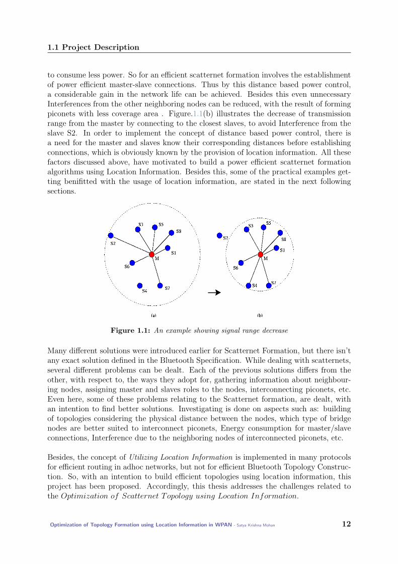
to consume less power. So for an efficient scatternet formation involves the establishmentof power efficient master-slave connections. Thus by this distance based power control,a considerable gain in the network life can be achieved. Besides this even unnecessaryInterferences from the other neighboring nodes can be reduced, with the result of formingpiconets with less coverage area . Figure.1.1(b) illustrates the decrease of transmissionrange from the master by connecting to the closest slaves, to avoid Interference from theslave S2. In order to implement the concept of distance based power control, there isa need for the master and slaves know their corresponding distances before establishingconnections, which is obviously known by the provision of location information. All thesefactors discussed above, have motivated to build a power efficient scatternet formationalgorithms using Location Information. Besides this, some of the practical examples get-ting benifitted with the usage of location information, are stated in the next followingsections.

Figure 1.1: An example showing signal range decrease

Many different solutions were introduced earlier for Scatternet Formation, but there isn’tany exact solution defined in the Bluetooth Specification. While dealing with scatternets,several different problems can be dealt. Each of the previous solutions differs from theother, with respect to, the ways they adopt for, gathering information about neighbour-ing nodes, assigning master and slaves roles to the nodes, interconnecting piconets, etc.Even here, some of these problems relating to the Scatternet formation, are dealt, withan intention to find better solutions. Investigating is done on aspects such as: buildingof topologies considering the physical distance between the nodes, which type of bridgenodes are better suited to interconnect piconets, Energy consumption for master/slaveconnections, Interference due to the neighboring nodes of interconnected piconets, etc.

Besides, the concept of Utilizing Location Information is implemented in many protocolsfor efficient routing in adhoc networks, but not for efficient Bluetooth Topology Construc-tion. So, with an intention to build efficient topologies using location information, thisproject has been proposed. Accordingly, this thesis addresses the challenges related tothe Optimization of Scatternet Topology using Location Information.


1.2 Applications of Location Based Services (LBS)

1.2 Applications of Location Based Services (LBS)

The combination of wireless networking and a location-based service (LBS) offers somevery interesting applications. LBS system helps to get the location of a particular user(or node) and integrate the position information into a wide variety of solutions.Applications in indoor areas using LBS are stated below :-

1. BlipZone : It is one of the examples for Location Based Service, that provideslocalised web-content and push messages to Bluetooth enabled mobile phones, handheld computers.[7]

Instantly send location dependent customised multimedia messages, offerings,and commercials to users as they enter and exit BlipZones. For example,

• In Restaurants :- Sending welcoming messages, offering information, web ac-cess, entertainement, when the guests are at the premises of the restaurants.

• In Shopping mall :- Provide information to shoppers about up coming events.

• In Public transportation :- Provide travel information, news and entertainment,and fill the idle minutes of busy travellers. The system automatically learnsthe movement patterns of frequent travellers, and sends out messages if theyare affected by delays.[7]

2. Tracking improves Security : An LBS system helps to track the users, assets etc.In hospitals, immediately born babies are attached with a tracking device. Withthe help of this device, sensors within that area track the location of the baby. Formonitoring baby movements, and for avoiding the theft of the born baby(s), thistracking facility can be used.

1.2.1 Reason behind mentioning of Location Based Services

All of the above quoted examples are applied, when the location of the Bluetooth units(i.e. users or nodes) are known.

In a similar fashion as of the above, all the Proposed Algorithms in this project areimplemented with an assumption that Location Information of the Bluetooth units areknown. So practical implementation of the proposed algorithms when the location isknown, can also considered as one of the applications of Location Based Service.

⇒ For example :- Customers in a restaurant, can be connected in a better fashion (in theway of Proposed Algorithms) either mutually in an ad-hoc mode (or) to the infrastructurenetwork placed in the restuarant.

The bottom line of this section is that, the method of connection of Bluetooth unitsusing Location Information, in the way of Proposed algorithms implemented on Bluetreealgorithm (discussed in futher chapters); can be also considered as one of the applicationsof Location Based Services.


1.3 Outline of the Report

1.3 Outline of the Report

The outline of the Project is of the following:

Chapter 2 will introduce about the history of Bluetooth and its technology. An overviewabout the topology of a scatternet and constraints needed for its efficiency are brieflystated. This chapter includes literature survey of scatternet formation algorithms andabout the chosen Bluetree algorithm. It will then be followed by Bluetooth Communica-tion and a background knowledge about Localization is described in Appendix.C.

Chapter 3 starts with a test case scenario consisting of a simple room model. Cho-sen Bluetree algorithm and different proposed algorithms using location information areexplained with flow diagrams. Parameters that are taken into account for performanceevaluation are presented in detail.

Chapter 4, compares the performances of all the algorithms by conducting simulationson the basis of characteristic metrics already stated in Chapter 3. For this some assump-tions have to be made , that are briefly stated at the starting of the chapter. Scatternetformation of the algorithms are represented for certain number of nodes (i.e. 60 nodes)and metrics such as Average Farthest Slave Distance, Collision Rate, Average ShortestPath Ratio are tested for different number of bluetooth nodes, slaves, simulation areas,respectively.

Chapter 5 presents the Conclusion and the Future Work.


Chapter 2Background

Introduction

This chapter will introduce about the history of Bluetooth and its technology. An overviewabout the topology of a scatternet, communication taking place within the bluetooth nodesand the constraints needed for scatternet efficiency; are presented. The chapter includesliterature survey of scatternet formation algorithms with detailed explanation of the chosenBluetree Topology. Background knowledge about Localization can be found in Appendix.C.

2.1 Bluetooth Technology

Bluetooth was introduced in 1994 by L.M.Ericsson of Sweden when it began researchingon the idea of cable replacement with wireless links. Out of the study for using radio linksto connect phones, headsets, computing devices etc has led to the release of BluetoothSpecification version 1.0 in 1999. It is further developed by a Bluetooth Special InterestGroup (SIG), formed by a group of five companies i.e., Ericsson, Nokia, IBM, Intel andToshiba. The specification is named after a Danish Viking monarch in the 10th CenturyA.D called Harald Blatand ’Bluetooth’, who united and controlled Denmark and Norway.Furthermore his unifying approach has led to his name adoption as Bluetooth which isexpected to unify the telecommunications and computing industries. [14]

Bluetooth wireless technology is a low-cost, low-power, short-range radio link that can beconveniently used for interconnecting all kinds of mobile and fixed devices. It is a Wire-less Personal Area Network technology (WPAN) operated in the unlicensed Industrial-Scientific-Medical (ISM) band at 2.4 GHz. In this band, it uses a slotted Time DivisionDuplex (TDD) protocol with a Frequency Hopping Spread Spectrum (FHSS) technique.Its transmission range varies from 10m to 100m depending on the output power trans-mitted.

Bluetooth devices can operate within two different networking frameworks:- Infrastructure mode, in which devices communicate with each other by first going throughan Access Point(AP).


2.2 Networking

- Ad-hoc mode, in which devices or stations communicate directly with each other, with-out using an Access Point. An Access Point is a device that acts as a communicationhub for users within a wireless network and can also serve as the point of interconnectionbetween the WLAN and a fixed wire network.[13]

Figure 2.1: An example for Bluetooth Network [16]

A simple example for wireless network connected with Bluetooth is depicted in Fig.2.1,showing the PDA, printer, audio system, mp3 player, computer etc connected with eachother via Bluetooth Technology.

2.2 Networking

This section gives an overview about the basic networking concepts, type of nodes usedfor interconnection of piconets, communication with bluetooth, characteristic metrics con-sidered in this project and Bluetree algorithm.

2.2.1 Topology Formation

As stated in Bluetooth specifications [9], when two BT nodes are in each others commu-nication range awaiting for the connection established between them, one of them mustassume the role of master and the other becomes its slave. The network established hereimplies a simple network called piconet and the master can accumulate not more thanseven active slaves at the same time. Bluetooth can be extended to interconnect mul-tiple piconets to create a multihop adhoc network called scatternet, consisting of largenumber of devices. Figure2.2 depicts a simple Bluetooth scatternet interconnected from3 piconets. With the frequency hopping spread spectrum technique(FHSS) employed byBluetooth, the 3 piconets communicate with each other at the same time and at the sameplace.


2.2 Networking

Figure 2.2: Bluetooth Scatternet [10]

Basically, bluetooth requires to solve various problems in adhoc networks from the net-working point of view,and out of which three of them stated as :

• Scatternet formation

• Scheduling of bridge nodes

• Routing in Bluetooth scatternets [2]

Out of these three, mainly Scatternet Formation problem along with Routing, are investi-gated in this thesis. The former one, is an open research problem and there is no specificmethod addressed in the standard for the interconnection of piconets to form scatternet.There are many topological alternatives to form a scatternet out of same group of devices.The way a scatternet is formed considerably affects its performance with respect variouscharacteristic metrics.

At first, Scatternet formation protocols are broadly classified into two topologies .i.e.a)single hop topology where all the nodes are in the radio vicinity of each other and theother is b)multi hop topology where there is no requirement for each node to be in thecommunication range of all other nodes. [11]

The algorithms in this project are based on the multihop scatternets providing connec-tivity over distances greater than the short radio range.

2.2.2 Bridge Node

When a large number of Bluetooth devices are in the proximity of each other, a scatternetis formed by interconnecting a number of piconets, together by sharing some commondevices known as bridge nodes. These act as gateways and forward traffic between the


2.2 Networking

adjacent piconets. This inter-piconet unit switches from one piconet to the other on atime-shared basis and it is limited to be a part of 8 piconets for simplicity [22]. Thenumber of piconets that bridge node participates is technically termed as number of rolesper node. In almost all the algorithms except Bluetree with Mesh, number of roles perbridge is 2. Basically these are classified into two types, namely Master-Slave (M/S)bridge and Slave-Slave (S/S) bridge. We come across these two bridges all through theproject for interconnection of tree topologies. An example figure showing the bridge nodesis in Fig .2.3.

Figure 2.3: Two types of bridge nodes, (a) M/S bridge, (b) S/S bridge

• Master-Slave (M/S) bridge :

M/S bridge node, depicted in Fig.2.3(a) acts as a slave in the Piconet 1 and asa master in the Piconet 2. As per the algorithms explained in next chapters, thisis short explanation of how the bridge nodes get connected with reference two pi-conets in the figure 2.3(a,b). Initially this bridge is acting as a slave for Piconet 1and communicates with master M1. After this, it assumes the role of master M2and get connected to the slave in Piconet 2.

• Slave-Slave (S/S) bridge :

This S/S bridge, depicted in Fig.2.3(b) acts as a slave in both the piconets. Thisbridge node acts as a slave to the master M1 in Piconet 1. It assumes the role ofslave to another Piconet 2, when it is paged by another master M2 of Piconet 2.Thus it acts as a slave in both the piconets, by switching on a time shared basis.

2.2.3 Bluetooth Communication

Communication in a piconet is organized so that the master polls each slave accordingto a polling scheme. A slave is only allowed to transmit after having been polled by the


2.2 Networking

master. The slave will start its transmission in the slave-to-master timeslot after it hasreceived a packet from the master. The master may or may not include data in the packetused to poll a slave.

1. Packets on the Physical Links :

Between master and slave(s), two types of connections can be established statedas:

• Synchronous Connection-Oriented (SCO)

• Asynchronous Connection-Less (ACL)

The SCO link is used for voice transmission. This application is used in real-timetwo-way communication. A point-to-point link is established between a master andonly one slave, and specific time slots at regular intervals are used. The latencytime is reduced as much as possible. In this mode, packets are never re-transmitted.The maximum throughput is 64 Kb/s full-duplex.[13]

The ACL link is used for non real-time transmission where data integrity is impor-tant. The packets are retransmitted until there are no more errors at the receptionor if an upper time limit is reached. That is why automatic repeat request is usedin this mode. Asynchronous connection can support symmetrical or asymmetrical,packet-switching, point-to-multipoint connections. In asymmetric connection, themaximum bit rate is 723.2Kb/s in one way and 57.6Kb/s in the other way. Insymmetrical connection, it is 433.9Kb/s in both ways.[13]

Figure 2.4: Multislave Operation using TDD [14]

2. Time Division Duplexing : The channel is the medium through which bluetoothunits communicate and is divided into timeslots of each 625µs in length. More


2.2 Networking

precisely, the Bluetooth system provides duplex transmission based on slotted Time-Division Duplex (TDD). The division by slot enables each member of the piconetto participate because TDD uses the same channel and continuously alternatesbetween sending and receiving as shown in Fig. 2.4. Master and slaves tranmitpackets alternatively in TDD scheme. The numbering of these slots ranges from0 to 227-1. As of these numberings, Master transmit in even numbered slots andthe slave in odd numbered slots. Slaves cannot exchange data among themselves,infact they have to contact only with the master or else they should form their ownindependent piconet. Packets tranmitted by either master or slave can range up tothe maximum of five time slots as shown in Fig.2.5. [14]

Figure 2.5: Multi-slot packets [14]

3. Frequency Hop Spread Spectrum :

Bluetooth uses Frequency Hop Spread Spectrum (FHSS) as an interference avoid-ance technique. The binary data in the baseband level of Bluetooth is modulated byusing Gaussian Frequency Shift Keying (GSFK). Then, they are transmitted usinga carrier determined by a frequency synthesizer.[13]

Instead of producing only a single carrier frequency, the synthesizer is controlledby a hop code generator that causes it to change carrier frequency at a nominal rateof 1,600 hops per second. One Bluetooth data packet is sent per hop. A Deviceuses one frequency in one timeslot. Then, by a frequency hop, it will change of fre-quency in the next timeslot and so on. Thus, for two Devices to communicate usingFHSS, they must be properly synchronized in order to hop together from channelto channel [13]. This means that the Devices must:

• Use the same channel set

• Use the same hopping sequence within that channel set


2.2 Networking

• Be time-synchronized within the hopping sequence

• Ensure that one transmits while the other receives, and vice versa (TDD prin-ciple) All of these synchronization parameters are determined by the piconetmaster. The master passes the FHSS synchronization parameters to a slaveduring the Page process. When an external Device wants to enter the piconet,it has to acknowledge this continuation of frequency hoping to be able to followit.[13]

4. States of Bluetooth Devices :

Figure 2.3 shows all possible states of a Bluetooth Device. There are two mainstates in the Bluetooth link controller: standby and connected.

• Standby state : is the default state in the Bluetooth unit. In this state, theBluetooth unit is in a low-power mode where the energy consumption of theDevice is highly reduced.

• Connected state : means that the Device participates in a piconet.

Figure 2.6: State diagram of Bluetooth device [13]

The others sub-states are:

• Inquiry : The master will search which units are in range, and what theirDevice addresses and clocks are to initialize the communication. This requestwill be repeated as long as a unit has not been found.

• Inquiry scan : used by a slave to listen to an Inquiry.

• Inquiry response : the state of the Device switches from the Inquiry scansubstate to the Inquiry response substate when it answers to the master Inquiryby sending its address and its clock state.[13]


2.2 Networking

After receiving the Inquiry response, a connection is established for the Pagingprocedure.

• Paging : is used by a master to establish a piconet with a particular slavewhose Bluetooth Device address is known.

• Page scan : is used by a slave to listen to its page. Slave response: state ofthe Device after receiving the message from the master for a connection. Thenthe slave will send its Access Code to the master.

• Master response : after the reception of the slave response, the master willsend a packet called Frequency Hopping Synchronization (FHS) which willpermit the slave to be synchronized with the master clock.

• Connected : The connection has been established and packets can be sentback and forth. The channel (master) Access Code and the master Bluetoothclock are used to determine the sequence of Frequency Hopping used in thispiconet.

• Active : The Bluetooth unit actively participates on the channel. The masterschedules the transmission based on traffic demands to and from the differ-ent slaves. Regular transmissions are made by the master to keep the slavessynchronized to the channel.[13]

Once connected, the unit is able to transmit and receive data. To save batterypower, three low power modes are available: Sniff, Hold, and Park (in decreasingorder of power efficiency). These modes are useful for:

- enabling more than seven slaves to be in a piconet- giving the master time to bring other slaves into its piconets- conserving energy

The main goal of these modes is to reduce the time for a Device receiver to remainon. The lower power level covers a distance of about 10 meters, while the higherpower level can cover about 100 meters.[13]

2.2.4 Characteristics of Scatternet Formation

One can signify that the efficiency of a scatternet is better, when it outperforms the othertopologies, with respect to the performances of particular characteristics. Definitions ofthe metrics adopted are stated as follows:-

1) Average Shortest Path : It is the average value of the shortest route lengthsbetween any two-nodes in a Bluetooth network. If a node wants to communicate in ascatternet, it is desirable to find a shortest path to the destination node i.e. less num-ber of hops, possible to consume less energy and thus an improved routing efficiency isobserved for a lower ASP value. The route length counted in hops gradually decreaseswith an increase in multiple paths. It can be also termed as Network Diameter definedas number of hops required between any two devices.


2.2 Networking

2) Average Farthest Slave Distance (AFSD): It is the average value of Farthestslave distances corresponding to all the piconets in a network. This parameter is relatedto the caliculation of master/slave connection ranges and is advisable to be less to de-crease the transmission power from the masters. A detailed explanation is given in thenext chapter. Let N be number of piconets, dFS be Farthest Slave distance of a piconet,then

AFSD =

∑NFS=1 dFS

N(2.1)

3) Collision Rate (CR): It is the ratio of number of packets lost to the total number ofpackets transmitted. Collisions occur when simoultaneous transmissions take place overthe same channel, from multiple nodes, which are in transmission range of each other.Such collisions are undesirable and lead to the wastage of energy, increase in data latency,etc.

Collision Rate (CR) =Number of Lost packets

Number of Total packets(2.2)

These metrics are referred with the following example:Consider a situation where a number of people gathered to watch a drama in a theatre (or)any other public places. In this new era of modern age, almost everybody are habituatedto carry bluetooth enabled portable devices like PDA, cell phones etc. They can form anetwork among themselves to send messages, pictures, transfer of files, etc. Neither thetime to get connected (nor) the number of piconets required to form a network, are notreally important in such a situation. Only thing is that, they need to be connected andactively communicate, without interference for a maximum duration possible. For this,power should be saved, which in turn may be possible by maintaining shorter range mas-ter/slave connections. Transfer of messages from one person to the other, by interactingwith less possible persons along the way, towards the destination person (i.e. shortestpath possible), is also evident. A more detailed explanation about these metrics is givenfurther in this report.

2.2.5 State of Art

Bluetooth Specification did not specify any particular method for scatternet formationand it is still an open issue. Many scatternet formation solutions are proposed before andthey are briefly stated to get an overall view. They can be broadly classified into twocategories such as single-hop topology ([17],[18],[19]) where all the devices are in the radiovicinity of each other and multi-hop topology ([10],[12],[20],[21]).

The solution presented in Bluetooth Topology Construction Protocol (BTCP)[17], is basedon leader election process to collect topology information. The leader decide on the rolesfor each other node by running a centralized algorithm. It is limited to single hop scenar-ios and number of nodes to be ≤ 36.

Besides, the solutions [18], [19] run over single hop topologies but there is no limita-tion on the number of nodes. G.F.Tan of [19] introduce TSF protocol(Tree Scatternet


2.2 Networking

Formation); the topology produced is a collection of one or more rooted trees try to mergetogether and converge to form a unique (one rooted) tree.

In the solution [10] called BlueNet, BT nodes collect information about its neighborsin the discovery phase and randomly enter page state (will become masters) to invitetheir neighbors for joining into their piconets. In case of any left nodes in first phase willbe connected in second phase and finally all of the piconets are interconnected. But atall the times, the connectivity of the resulting scatternet is not guaranteed.

Bluemesh [20], is in two phases and in the first phase two node temporary piconets areestablished at every node pair to exchange information symmetrically. After having alocal list of all its neighbors, a node exchanges this list with its neighbors, thus obtainingtwo-hop neighbor hood knowledge. Next phase is scatternet formation which proceedsin iterations where in each iteration master chooses seven slaves (in case of >7) thorughwhich it can reach all the others(i.e. two hop neighbors). After the selection of masterand slaves, gateways are selected to join adjacent piconets to form as scatternet.

Bluestar [21] is organised in three phases such as topology discovery, BlueStar forma-tion and configuring of BlueStars - The Blue Constellation. In the first all the devicesdiscover each other by establishing temporary piconets with their neighbors. Relying onthe sole knowledge of neighbors, they decide whether they are fit to serve as a master ornot. Once piconets are formed, gateway nodes are selected to interconnect themselves.At the last, there is Bluetree algorithm[12] explained in the further sections.

The project doesn’t deal with an introduction of a new scatternet formation protocol,but it is with Optimization of already existing protocol. For this reason, an algorithmhas to be chosen out of all the algorithms discussed earlier. Algorithms relating to Singlehop topologies are not always good to implement when there is mobility with the nodes.So presently they are out of discussion.

Out of multihop topology solutions, Bluetree algorithm is selected which is feasible forboth centralized and distributed approaches. It is basically a Centralized topology, whereone node acts as a gate-way to another network. In order to communicate with other net-works, the other nodes will obviously need to be connected to this node; thus resulting in atree topology (Example: Internet, Blip Net). Figure.2.7 resembles Tree topology networkwith two Blip Nodes acting as route nodes to their own clients, and these client nodesaccess the other networks, through these Blip nodes (acting as gateways). BlipServermonitors entire BlipNet and acts as route node to the whole network. Applications ofBlipNet ( i.e. Location Based Services mentioned in Chapter 1) and its resemblance tothe Tree Topology, has led to the point of thought that, Bluetree algorithm is well suitedalgorithm for further investigation.


2.2 Networking

Figure 2.7: Blip Net resembling Tree Topology [3]

2.2.6 Bluetree Algorithm

Let us assume that Bluetooth nodes are randomly distributed in a given geographic regionawaiting to form a scatternet among them.

Assumptions for connection establishment :

1. Nodes remain static where they are placed

2. Boot process is the time during which all their neighbors get discovered from in-quiries and responding to inquiries. So it is assumed that boot process is completed,after which every node is well aware of the number and identities (i.e., the Bluetoothaddress) of each of its neighbors

3. Any two nodes can be said to be neighbors if they are within each others transmissionrange, and there is at least one path between them in the ’geographically connected’network. [12]

Scatternet formation starts with a given single node called the blueroot. It is an arbitarynode assumed here to be selected out of all the nodes spread in the geographic region. Arooted spanning tree from the blueroot is built using the network topology graph and arole of master (M) is assigned to it. Blueroot acquires all its one-hop neighbors as slaves(S) but not more than 7, to form the piconet. This is depicted by drawing a directed linkfrom the root to its children. These children will now be assigned an additional role M


2.2 Networking

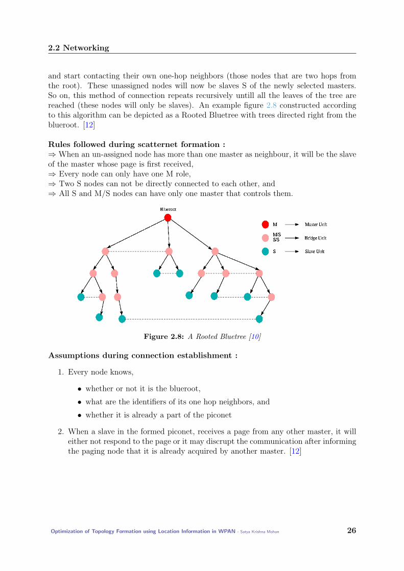
and start contacting their own one-hop neighbors (those nodes that are two hops fromthe root). These unassigned nodes will now be slaves S of the newly selected masters.So on, this method of connection repeats recursively untill all the leaves of the tree arereached (these nodes will only be slaves). An example figure 2.8 constructed accordingto this algorithm can be depicted as a Rooted Bluetree with trees directed right from theblueroot. [12]

Rules followed during scatternet formation :⇒ When an un-assigned node has more than one master as neighbour, it will be the slaveof the master whose page is first received,⇒ Every node can only have one M role,⇒ Two S nodes can not be directly connected to each other, and⇒ All S and M/S nodes can have only one master that controls them.

Figure 2.8: A Rooted Bluetree [10]

Assumptions during connection establishment :

1. Every node knows,

• whether or not it is the blueroot,

• what are the identifiers of its one hop neighbors, and

• whether it is already a part of the piconet

2. When a slave in the formed piconet, receives a page from any other master, it willeither not respond to the page or it may discrupt the communication after informingthe paging node that it is already acquired by another master. [12]


2.3 Conclusion

2.3 Conclusion

Bluetooth is a low-cost, low-power device feasible for short-range wireless personal areanetwork technology. In the netwoking point of view, basic concepts such as piconet, scat-ternet, contribution of different types of nodes are briefly stated. Bluetree Algorithmis chosen out of various scatternet formation algorithms and the background knowledgeabout its working is clearly explained. Bluetooth units communicate among each otherby employing TDD scheme and they fall into different states such as Inquiry, Inquiryresponse, Paging etc to establish connections. From the Appendix.C, we can know howthe position of a device can be known by certain location techniques such as Cell Iden-tification, Angle of Arrival, Signal Strength, Uplink Time of Arrival, etc. and infact,knowing location information through these techniques ,finds several real time applica-tions. The next chapter follows with implementation of such location information onBluetree algorithm in the form of different solutions and their analysis.


2.3 Conclusion


Chapter 3Proposed Algorithms

Introduction

This chapter starts with a test case scenario consisting of a simple room model. Cho-sen Bluetree algorithm and different proposed algorithms using location information areexplained with flow diagrams. Parameters that are taken into account for performanceevaluation are presented in detail

3.1 Scenario Description

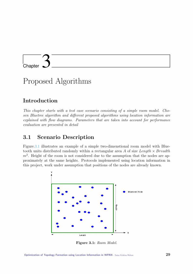
Figure.3.1 illustrates an example of a simple two-dimenstional room model with Blue-tooth units distributed randomly within a rectangular area A of size Length × Breadthm2. Height of the room is not considered due to the assumption that the nodes are ap-proximately at the same heights. Protocols implemented using location information inthis project, work under assumption that positions of the nodes are already known.

Figure 3.1: Room Model.


3.1 Scenario Description

The theme of the project is not, how we can get location, but what is the benifit after weget location information. It is like next further step of acquiring positions of Bluetoothunits. The benifit in this project, with the use of location information is related to theOptimization of already existing scatternet formation protocols. One of them is:

Bluetree Formation Protocol can be applied in two different approaches i.e.

1. Centralized approach : It is based on a designated node, Blueroot, that initiatesthe construction of a bluetree, i.e., the resulting scatternet topology will be a treethat spans the entire network.

2. Distributed approach : It speeds up the scatternet formation process by selectingmore than one root for tree formation, and then merging the trees generated byeach root. This protocol is organized in two phases. In the first phase, a subset ofthe nodes will be selected as initnodes that initiate the construction of subtrees,similar to the first algorithm. In the second phase, the protocol merges the generatedsub-trees into one scatternet that spans the entire nework.[24]

Both of the approaches are almost the same, but a)merging of piconets and b) fastformation of the scatternet compared to Centralized approach; are the additional thingsdone in the Distributed approach. For the sake of simplicity, clear understanding of thetopologies from the figures and to do more research, I have opted for the Centralizedapproach in this project.

Things to be noted :

1. Parameters for reference, that come across during the explanation of further protocols:-

• Bluetooth range i.e BTrange= 10 m

• Maximum number of slaves per piconet i.e Smax = 7

• Number of nodes = N

2. As you already know, Centralized approach is opted for Perfomance evaluationof all the algorithms. In this, scatternet formation starts with only single nodecalled Blueroot. The selection of Blueroot either can be an arbitary node (or) canbe a predefined node connected to a Local Wired Network, technically termed asInfrastructure mode. Well the first case is adopted .i.e. an arbitary node selectionacting as Blueroot in all the further sections.

3. The explanation of the following algorithms depicts, what is done during the simula-tions, for the construction of scatternets. Bluetree Algorithm without using LocationInformation, is explained again in the next section apart from the previous chapter.Here, it is according to the simulator programmed, assissted with flow diagrams.


3.2 Bluetree Algorithm


To start the tree formation, a random node out of all nodes distributed within the room,is selected to act as Blueroot.

Step1 : Blueroot is assigned the role of Master, starts to search for the nodes within theBluetooth range. It searches and connects immediately until it has got 7 children. Thechildren of Blueroot are now assigned the role of Slave.

Figure.3.2 shows the Flow diagram of all the steps untill all the nodes get connected.

Figure 3.2: Flow Diagram - Bluetree without Location using S/M bridges.[24]

Step2 : Slaves of the Blueroot are now assigned an additional role of Master, thusacting as bridge nodes. Now each bridge node of Step2, start the searching procedure toconnect to the unassigned nodes.

• Each bridge node searches and immediately connects after each search of unassignednode within Bluetooth range. Each bridge node can connect to maximum of Smax

slaves.

• One bridge node’s turn for search, comes only after the completion of the entireunassigned nodes search of the other bridge node. In simple terms, until first bridgesearches all the unassigned nodes, the second bridge doesn’t get a chance to search.



• If the first bridge has already got 7 slaves, before all the unassigned nodes search; itimmediately passes the turn to second bridge, without searching for the remainingnodes.

Assumptions :⇒ Master searches only for the unassigned nodes. Once a node is part of a piconet, itcannot be connected to the second Master even though if it is within range of secondMaster. Simply to say node can be a Slave to only One Master.

Step3 : The same procedure in Step2 continues until all the nodes are assigned topiconets.

An example of a scatternet formed with 60 nodes randomly distributed in a squareroom of 30 meters, following this algorithm i.e. Bluetree without Location Informationusing S/M bridges is shown in Figure.3.3. Same node positions are taken for comparisonof all the scatternet topologies.

Figure 3.3: Bluetree without Location using S/M Bridges.


3.3 Proposed Scatternet Formation Algorithms exploiting LocationInformation

3.3 Proposed Scatternet Formation Algorithms ex-

ploiting Location Information

3.3.1 Bluetree with Location Information - 1

1. Scatternet Formation with Slave-Master Bridges

Procedure is same as Bluetree until the selection of Blueroot.

Step1 : Blueroot is assigned the role of Master, starts to search for the nodeswithin the Bluetooth range. It searches all the nodes within range and doesn’timmediately connect as of Bluetree algorithm. After the completion of searching,Blueroot picks up all the nodes within range and connects to the closest 7 i.e Smax

nodes out of all. All the connected nodes in this Step are assigned the role of Slave.Figure.3.4 shows the Flow diagram of all the steps untill all the nodes get

connected.

Step2 : Slaves of Step1 are now assigned an additional role of Master, thus actingas bridge node (S/M). It is an assumption that every node after being a part of apiconet, an additional Master role is assigned which in turn start paging its one-hopneighbors (and in this algorithm, it cannot assume an additional Slave role insteadof Master because the algorithm is designed for S/M bridges). Each bridge nodestart searching and connecting one after another. These nodes play the same rolefor connection as of Blueroot in Step1.

• Bridge nodes search all the unassigned nodes within range and connect to theclosest Smax nodes. After the complete search and connection of one bridgenode, then comes the turn for search of the next following bridge node. Insimple terms, each bridge node search and connect to the maximum of Smax

slaves, one after another.

Assumptions :⇒ Slave can be connected to only one Master. Once a node is part of a piconet, itcannot be connected to another Master.Step3 : The same procedure in Step2 continues until all the nodes are assigned

to piconets.

An example of a scatternet formed with 60 nodes randomly distributed in a squareroom of 30 meters, following this algorithm i.e. Bluetree with Location-1 using S/Mbridges is shown in Fig.3.5.



Figure 3.4: Flow Diagram - Bluetree with Location-1 using S/M bridges.



Figure 3.5: Bluetree with Location-1 using S/M Bridges.



2. Scatternet Formation with Slave-Slave Bridges

Figure 3.6: Benifit of using S/S bridges.

In this algorithm S/S bridges are used instead of S/M bridges. Figure.3.6 illustratesan example of 4 nodes connected by S/M, S/S bridges. For the same set of nodes toget connected, S/M bridges requires 3 piconets, and S/S requires 2 piconets, whichoverlap with each other. By the usage of S/S bridges, the number of overlappingpiconets reduced from 3 to 2 and as a result, less number of collisions are expectedthan with the usage of S/M bridges. For case(a) average farthest slave distance istaken for 3 slave distances from 3 piconets , whereas in case(b) it is taken for 2distances. So even there is a possibility of decrease in the average, for less numberof distances. With a hope that there may be an improvement in both collision rate,average farthest slave distance, S/S bridges are introduced.

Procedure is same as of the above algorithm using S/M bridges untill the com-pletion of Step 1. At the end of this Step, Blueroot has maximum of Smax closestslaves.


Step2 : The slaves formed in Step1 need to be paged by another masters to assumethe role as S/S bridges. The selection of masters to page these slaves can be donein different ways and here they are selected on the basis of the closest node. Itis an assumption that, each corresponding closest node(unassigned) of every slaveis assigned the role of Master and connects to them. So now every Master hasone slave and still six more slaves can be connected. Each Master node now startsearching and connecting one after another. These master nodes play the same rolefor connection as of Blueroot in Step1.

• Master nodes search all the unassigned nodes within range and connect tothe closest Smax − 1 nodes. After the complete search and connection of onemaster node, then comes the turn for search of the next following master node.In simple terms, each master node search and connect to the maximum ofSmax − 1 slaves, one after another.


An example of a scatternet formed with 60 nodes randomly distributed in a square



Figure 3.7: Flow Diagram - Bluetree with Location-1 using S/S bridges.

room of 30 meters, following this algorithm i.e. Bluetree with Location-1 using S/Sbridges is shown in Figure.3.8.



Figure 3.8: Bluetree with Location-1 using S/S Bridges.




In the previous algorithm, the turn for one master comes only after the other mastermakes all the possible connections. If it is like this, there is a chance that some slaveswho assumed the role of master (i.e. S/M) doesn’t have any unassigned nodes to connect.To build a more balanced tree, in such a way that every master gets a chance to connectto an unassigned node, if it is within the coverage area; this algorithm is proposed witha hope that Location Information-2 is an upgraded algorithm of Location Information-1.


This algorithm is a slight modification of Bluetree-Location1. It follows Location1algorithm until Step1 procedure. After the completion of Step1, Blueroot has max-imum Smax slaves.


Figure.3.9 shows the Flow diagram of all the steps untill all the nodes get con-nected.



Step2 : From here, the algorithm slightly differs from Bluetree-Location1. Theslaves formed in Step1, are assigned an additional role of Master, acting as bridgenodes with S/M role. These bridge nodes now start the searching procedure. Eachbridge node searches and connects only to a single node one after another. Eachbridge node searches all the unassigned nodes and picks up all the nodes withinrange. Out of these nodes, only one closest node to bridge node is selected andconnected to it. The following next bridge nodes repeat the same procedure. Itcompletes one cycle after all the bridge nodes gets their chance to have first child.This method of search and connection repeats for 7 i.e Smax, number of cycles. Afterall the Smax cycles, Step2 is completed.

Step3 : The same procedure in Step2 is repeated until all the nodes are assignedto piconets.

An example of a scatternet formed with 60 nodes randomly distributed in asquare room of 30 meters, following this algorithm i.e. Bluetree with Location-2using S/M bridges is shown in Fig.3.10.





In this algorithm, S/S bridges are used instead of S/M bridges. Procedure is sameas of the above algorithm using S/M bridges untill the completion of Step 1. At theend of this Step Blueroot has maximum of Smax closest slaves.



Step2 : The slaves formed in Step1 need to be paged by another masters to assumethe role as S/S bridges. The closest nodes of S/S bridges are selected as mastersand get connected. So now every Master has one slave and still six more slavescan be connected. Till here in this Step, the procedure is same as that of Bluetree-Location-1 using S/S bridges. After this, the method of master connecting to theslaves is slightly different. These masters play the same role, as that of masters



in the Bluetree-Location-2 using S/M bridges. Master nodes start the searchingprocedure on all the unassigned nodes and picks up all the nodes within range. Outof these nodes, the closest node to the master is selected and connected to it. Eachmaster search and connect only to a single node one after another i.e. master afterconnecting to a single node, it gives the turn to the next following master. The fol-lowing masters repeat the same procedure. One cycle completes after every mastergets a turn to have its second child. This method of search and connection repeatsfor 6 i.e. Smax − 1 number of cycles. After all Smax − 1 cycles, Step2 is completed.



An example of a scatternet formed with 60 nodes randomly distributed in asquare room of 30 meters, following this algorithm i.e. Bluetree with Location-2using S/S bridges is shown in Figure.3.12.




In the previous two algorithms (i.e. Bluetree with Location- 1,2), we do not see slavesalways connecting to the closest masters. They connect to the masters, who page firstand also if it is one of the closest slaves only to that particular master. In another words,a slave may be closest to a master but in some situations, that master may not be theclosest one out of all other masters, to that slave. Eventhough such a slave is morecloser to any other master it couldn’t connect. In order to prevent such situations, thisalgorithm is proposed. Here, every master before connecting to its closest slave, checkswhether it is more closest to other masters or not. In case if it finds that particular slaveis more closest to any other master, it won’t connect and continues its search. So here,the shortest distant nodes or Only closest nodes, implies that they are closest from theperspective of both master and slave. Whereas in Location-1,2 algorithms, closest nodesimplies that they are closest from the perspective of only master.


In this algorithm, nodes get connected Only to the closest nodes. This is differ-ent when compared to all the other algorithms and it differs right from Step2 ofscatternet formation, in general. The same procedure as in Bluetree-Location (1)or (2) is followed until Step1. After Step1, Blueroot connects to the closest Smax

nodes within range. These nodes act as slaves to Blueroot.


Step2 : These slaves are assigned an additional role of Master acting as bridgenodes (S/M) nodes. For the bridge nodes to establish connection, two conditionshave to be satisfied before each and every connection.

• A Bridge node can connect to an unassigned node only, if that node from thepresent bridge node, is at the shortest distance when compared to all otherbridge nodes.

• If there are more than Smax nodes satisfying the above condition, to the samecorresponding bridge node, then the bridge node connects to the closest Smax

nodes out of these shortest distant nodes.


An example of a scatternet formed with 60 nodes randomly distributed in a squareroom of 30 meters, following this algorithm i.e. Bluetree with Location-3 using S/MBridges is shown in Fig.3.14.










Even in this algorithm, nodes get connected Only to the closest nodes or the short-est distant nodes. Only difference apart from previous algorithm is that, Location3with S/M bridges is replaced with S/S bridges. The same procedure as in Bluetree-Location3 with S/M bridges is followed until Step1. At the end of Step1, Bluerootget connected to the closest Smax nodes within range. These nodes act as slaves toBlueroot.


Figure.3.15 shows the Flow diagram of all the steps untill all the nodes get con-



nected.Step2 : In this Step, Master is chosen in a different way compared to previousLocation-1,2-(S/S) algorithms. With an intention to use ’Shortest Distance’ con-cept, the shortest distant nodes from the slaves of Step1 are selected as Masters.But here, to say an unassigned node is at a shortest distance from the correspondingslaves of Step1, two conditions have to be satisfied:

• An unassigned node is at the shortest distance, from the corresponding slave,when compared to all other slaves of Step1.

• If there are more than One unassigned nodes satisfying the above condition,the closest out of all the shortest distant nodes to the corresponding slave, ischosen.

These unassigned shortest distant nodes corresponding to each slave, act as Masters,thus establishing S/S bridges. Presently, Masters in this Step have only one slaveand can have more slave connections until Smax slaves.For the remaining master/slave connections, the following conditions have to besatisfied

• A Master node can connect to an unassigned node only, if that node from thecorresponding Master is at the shortest distance when compared to all otherMasters.

• If there are more than (Smax − 1) nodes (one slave is already connected)satisfying the above condition, to the same corresponding Master, then Masterconnects to the closest (Smax − 1) nodes out of these nodes.


An example of a scatternet formed with 60 nodes randomly distributed in a squareroom of 30 meters, following this algorithm i.e. Bluetree with Location-3 using S/Sbridges is shown in Fig.3.16.






3.3.4 Bluetree with Mesh Structure

All the algorithms discussed till now corresponds to every single slave connected withonly one master i.e. no two masters can establish connection with the same slave (ex-ception: Only for S/M bridges based algorithms). This condition is considerably alteredin the Mesh structures, where more than one master can access the same slave. In dy-namic environments, nodes arrive and depart arbitarily and thus, there is a chance ofloosing connections. In such situations mesh structures helps to find alternate paths tothe lost nodes. Following algorithms are for Mesh structures With and Without usingLocation Information ; and they use only Slave/Master bridge nodes during the scatternetformation.

1. Scatternet Formation without Location Information

This algorithm is entirely just like the basic Bluetree, with only slight modifica-tion in Step2 and in further Steps. The assumption right from Step2 in Bluetreealgorithm is that a slave can only be connected to one Master. But in this algorithm,this assumption is just removed; that implies different masters can connect to thesame slave in case if it is within the bluetooth range. Further Bluetree-Mesh, can bebetter modified if this assumption is taken as a varying parameter in the simulations.

For example: Let the varying parameter be msc (msc ⇒ master slave connection).When msc = 1 then, every slave can be connected to only 1 Master, and msc = 2then, slave can be connected to 2 Masters etc.So when msc = 1, Bluetree-Mesh behaves like Bluetree algorithm. Maximum valueof msc can be 7 in case of mesh networks why because maximum number of bridgenodes are 7 who assume the role of master.


An example of a scatternet formed with 60 nodes randomly distributed in a squareroom of 30 meters, following this algorithm i.e. Bluetree-Mesh without Locationusing S/M bridges is shown in Figure.3.18.



Figure 3.17: Flow Diagram - Bluetree - Mesh without Location using S/M bridges.



Figure 3.18: Bluetree-Mesh without Location using S/M Bridges.



2. Scatternet Formation with Location Information - 1

This algorithm is also entirely like Bluetree using Location Information -1, witha slight modification as of the above one. An example, showing 60 nodes got con-nected with this, is in Figure. 3.19.

Figure 3.19: Bluetree-Mesh with Location-1 using S/M Bridges.

3. Scatternet Formation with Location Information - 2.

This algorithm is also just like Bluetree using Location Information -2, with themodification as of the above. Even for this, a scatternet formed of 60 nodes isshown in Figure. 3.20. Performances of these are compared in the next followedchapter.


3.4 Characteristic Metrics

Figure 3.20: Bluetree-Mesh with Location-2 using S/M Bridges.


The set of metrics identified in the literature are the measures of the quality of a scatternet.In this section three different metrics are discussed for evaluating the performance of ascatternet, after it has formed. They are Average Farthest Slave Distance, Collision Rate,Average Shortest Path Ratio.

3.4.1 Average Farthest Slave Distance (AFSD)

Farthest Slave Distance(FSD) is the distance from a Slave, which is placed at a farthestdistance of all the slaves in a piconet, from the Master node. This metric is calculatedwith an intention to estimate the Power control, which is directly proportional to thedistance up to which power is transmitted, from the master in a piconet. Based on thedistance based power control, this metric should be less, as much as possible in order to



consume less power. [4]Equations.3.1,3.2 shows the proportionality between Power and Distance.

For T-R Distance >8 meters

PRx = PTx − PL = 0dBm− (58.3 + 33 ∗ log10(D/8))dBm[26] (3.1)

For T-R Distance <8 meters

PRx = PTx − PL = 0dBm− (20 ∗ log10(4 ∗ π ∗D/0.1224))dBm[26] (3.2)

whereD = Tx-Rx distancePRx = Power ReceivedPTx = Power TransmittedPL = Path Loss

3.4.2 Collision Rate (CR)

This section focusses on the measure of inter-piconet interference in terms of CollisionRate.

Condition for Overlapping piconets :Figure 3.21 illustrates the behaviour of piconets with respect to each other in all the 3Cases, based on the Farthest Slave Distance (FSD) theory stated before.

For example let us consider :-Piconet of interest = Piconet 1Interfering piconet = Piconet 2Farthest Slave Distance of Piconet 1 = RFSD1

Farthest Slave Distance of Piconet 2 = RFSD2

Distance between Masters of both piconets = DM

The two piconets doesn’t overlap with each other in Cases 2 and 3 satisfying the Equa-tion.3.3. These two cases can can not be considered as testing cases for Interferencebetween them.

DM ≥ RFSD1 + RFSD2 (3.3)

Graphical representation of the Case 1 satisfying the condition in Equation.3.4, impliesboth the piconets are overlapping with each other, resulting in a chance of interferencebetween them.

DM < RFSD1 + RFSD2 (3.4)

Interference, however, is not guaranteed by just the interferers (Piconet 2) presence. In-terference can only occur when the piconet of interest and at least one interfering piconethop to the same frequency during the same time slot. In order for this to occur, bothpiconets must be in the process of transmitting and receiving besides satisfying the Equa-tion.3.4.



Figure 3.21: Cases showing when Piconets Overlap.

Thus, when piconets hop to the same frequency during the same time slots, packetscollide with each other and get lost. This results in the retransmission of the packets.Collision rate is caliculted from Eq.3.5.

Collision Rate (CR) =Number of Lost packets

Number of Total packets(3.5)

=⇒ Assumptions :

• Simulations are assumed to be done for single slot transmissions in multiple piconetsthat would interfere with one another in time.

• All the piconets are synchronized to each other.

• All transmissions are symmetric.

1. Collision Rate considering Transmission in every slot :

Bluetooth transmits data in the form of packets. The channel is divided into timeslots of 625µs each and packets are transmitted in these time slots. Time DivisionDuplex(TDD) scheme is used in the Bluetooth system where master transmits ineven numbered slots and slave transmits in odd numbered time slots. This duplextransmission is just not represented in both the example figures 3.22, 3.23 for con-venience, i.e. only slots of transmission are shown for simplicity.



Figure 3.22: Example: Inter Piconet Interference for assumed Transmissions in every slot.

Piconets are assumed to be transmitting Single slot symmetric data packets at everytime slots as shown in Figure.3.22. In this figure, there are some slots where trans-missions from both the Piconets 1 and 2 are taking place at the same hop frequencyand some at different hop frequencies. Collision occurs for transmissions on thesame hop frequency, resulting in a piconet interference.

2. Collision Rate considering Transmission in random slots :

This case is slightly bit different than the above. It is not realistic to assume thatall the time slots will in transmission state, at every situation. So here, transmis-sions are not observed at every time slot. Depending upon the number of nodesin a piconet, Transmissions are assumed to be taking place in random slots. Moreprecisely, Equation.3.6 defines the probability of number of slots that can be intransmission state with reference to the number of nodes in a piconet. In simula-tions, this many slots are assumed randomly in transmission state from both thepiconets and tested for interference occurence.

Number of slots in Transmission state =Number of Nodes in a piconet

8×Total time slots

(3.6)

In Figure.3.23, two states are observed i.e. Transmission state and Idle state. Colli-sion occurs only when transmission takes place from both the piconets at the samehop frequency. If either of them is in Idle state, collision doesn’t occur.



Figure 3.23: Example: Inter Piconet Interference for Transmissions in random slots.

3.4.3 Average Shortest Path Ratio (ASP)

An overview about Visibility graph network and Dijkstra algorithm, are needed to beknown before caliculating Average Shortest Path Ratio i.e. ASPo. For this they arestated as below :

1. Visibility Graph :

For a given set of Bluetooth units, that are spread randomly in a specific geo-graphical region, a visibility graph network is defined as a network consisting of allthe units and all the potential links within the Bluetooth’s radio range.

Initially before establishing connections, all the nodes are void i.e., there is nei-ther a master nor a slave in any piconet.During the Inquiry process every Bluetoothnode collects information about its neighbours (irrespective of the number of neigh-bours) within radio range and forms a local visibility graph.[23]

Figure.3.24 shows the Visibility graph network of 60 BT nodes (note: positioned atsame places as in the example figures, of the algorithms explained before).

2. Dijkstra Algorithm :

There are different algorithms that can be used to solve the problem of findingthe shortest path. Out of them, Dijkstra Algorithm is one of the most efficient onesimplemented here to find Average Shortest Path Ratio. It is introduced by a Dutchcomputer scientist, Edsger Dijkstra in 1959. In general, with this algorithm, theminimum distance can be found from one given node of a network, called sourcenode, to all other nodes in the network.



Figure 3.24: Visibility Graph.

Let us see the terminology, before the explanation of how it works, with a simpleexample. Every node in the network is associated with a label, which representsdistance (cost) from source vertex to any other particular vertex. It is classified intotwo categories. One is temporary label given to the vertices that are not reachedand the value given to it can be varied. Second one is permanent label, given tovertices that are reached and the value given to it is the cost of that vertex to thesource vertex. [27]

In Fig.3.25(a), let A be the source node(vertex) associated with permanent la-bel of value 0, and all others with temporary labels of value 0. Next step is to theselect least cost edge connecting the source vertex to a temporary label vertex. Herein Fig.3.25(b) it is vertex B, changed to permanent label with a value 2, i.e. vertexA value + cost of edge from A to B. Next is to find least cost edge either from Aor B, which leads to permanent label of C with value 3. The procedure continuesuntill all the nodes have permanent labels. Finally as per Fig.3.25(d) node D is withpermanent label, composed of least cost edges connecting the nodes from A-B-D. [27]



Figure 3.25: Example for Dijkstra Algorithm [27].

Average Shortest Path Ratio (ASP) :

The ASP metric is defined as, the average shortest path-length (hop counting) amongall the 2-node pairs, in a Bluetooth network. It can be calculated using any shortestpath algorithm. Here in these simulations, Dijkstra algorithm is adopted. ASP ratio isthe metric to be compared and for this, ASP of Visibility graph is needed to be known.Visibility graph is formed when all the nodes get connected to each and every other nodewithin range, without any assumptions. All the possible potential links are utilized. Ob-viously for a given set of Bluetooth nodes, the minimal average shortest paths among allthe node pairs is formed, termed as ASPo from Eq.4.1. Usually, scatternet network hasless potentials links and so it is almost certain that ASP of the formed scatternet by anyalgorithm will be larger than ASPo.[23]

ASPratio =ASPo

ASPsct

(3.7)

where ASPsct is the actual ASP of the scatternet to be evaluated.

Generally ASP of a scatternet improves (i.e. it decreases or ASP ratio increases) withthe increase in number of potential links and it is observed in Set2 algorithms such as


3.5 Conclusion

Bluetree-Mesh, Bluetree-Mesh-Location-1,2 algorithms. Due to more links, Collision Rateand AFSD are expected to high in these three, when compared to all other algorithms.So if these increased links are connected with closest possible distances, CR and AFSDcan be decreased without much sacrifice of ASP ratio. Set1 algorithms such as Bluetree-Location-1,2,3 are proposed with an intention to decrease CR,AFSD and the ASP ratioof these can not be higher than Set2. Besides, ASP ratio can be comparable within theSet1 proposed algorithms.

3.5 Conclusion

A simple test case scenario is taken with a two-dimentional room model, consisting ofrandomly placed nodes. A Centralized approach is adopted where the scatternet formationstarts with a single node called Blueroot. Bluetree forms the basis of all the protocols ; andBluetree with Location Information -1,2,3 for both S/M , S/S bridges ; and finally Bluetreefor Mesh networks with Location Information -1,2 are all analysed with flow diagramsand sample figures. Characteristic metrics such as Average Farthest Slave Distance,Collision Rate, Average Shortest Path Ratio are briefly explained. Simulations resultsof the protocols based on these metrics are presented in the next chapter to compare andevaluate their performances.


Chapter 4Simulation Results

Introduction

This chapter initially explains about the test case environment. It is followed with apresentation of all the topologies discussed in the previous chapter. Their performancesare compared on the basis of characteristic metrics with different test cases like varyingnumber of slaves, size of the simulation area, total number of bluetooth nodes, contributingfor the formation of scatternet.

4.1 Simulation Environment

A single room is plotted with Bluetooth nodes randomly distributed; that are awaitingfor scatternet formation.

The following parameters of Bluetooth network are varied and are taken the same fordifferent protocols during simulations to evaluate their performances :-

Value DescriptionN 5 - 60 Total number of BT nodes

X × Y 20 × 20 - 45 × 45 Simulation Area i.e. SA (meter2)BTrange 10 Bluetooth radio range (meter)Smax 2-7 Maximum number of Slaves per piconet

Table 4.1: Parameters of Bluetooth Network

Assumptions made during the simulation of different algorithms :-

• A Two-dimensional room model in x-y plane is taken with no fixed dimensions. Theyare even varied during simulations for testing of different characteristic metrics, butthe size of the area is fixed for one simulation run.

• Both Length and Breadth of the Simulation area are taken equal, for uniform dis-tribution of randomly placed nodes.


4.2 Comparison of Topology Formation

• Maximum Simulation area for BTrange = 10m is 45 × 45 sq.mtrs(approx). Thisassumption is made to ensure that all the nodes get connected. In case if we simulatefor higher simulation areas, some nodes are left unconnected due to the fact theyare placed out of range from any of the nodes. It’s not possible to connect those byany means unless Bluetooth’s range is increased.

• Nodes are assumed to be placed at the same height and remain stationary duringthe simulation.

• For simplicity free space propagation model is assumed, which ensures that nodeswithin a certain distance will always be within radio range.


A detailed explanation is given in the previous chapter about the formation of topologies.To have an overview at a stretch, about how the topologies look like, figures of all thetopologies for N = 60 are again placed side by side. Out of all protocols, only in Bluetreewith Location-3-SM (Fig.4.6) and Bluetree with Location-3-SS (Fig.4.7), the connectionsi.e. lines doesn’t overlap with each other, pictorially. As it is a wireless scenario, it is notgood to say as Overlapping of Lines, but pictorially the connections among nodes, lookvery distinguished. And they imply that the piconets overlap less with each other; thusInterference can be reduced by using Space Division Multiplexing principle. This is notthe case with the other protocols in Figures.4.1, 4.2, 4.3, 4.4, 4.5.

Figure 4.1: Bluetree without Location using S/M Bridges



Figure 4.2: Bluetree with Location-1 using S/MBridges

Figure 4.3: Bluetree with Location-1 using S/SBridges







4.2.1 Simulation and Performance Evaluation

Simulations and development of the algorithms is done in MATLAB . Scatternet samplesare generated for BT nodes ranging from 5 to 60 and for the comparison purpose theyare generated from the same random seed. Each seed generates the same set of randomnumbers. With the usage of same random seeds, the postion of the nodes will be thesame for all the algorithms, which is needed for the comparison purpose. For good ap-proximation of the measured parameters, the results are averaged over 10 simulation runs.Besides this, simulator can work for any number of nodes such as 80, 100, 120 etc, andeven for more number of simulation runs; but it does consume much time to run. Sizeof the Simulation Area (SA), Maximum number of slaves per piconet (Smax), Number ofnodes (N) are varied in simulations to compare the results in all directions.

1. Average Farthest Slave Distance

This value is obtained by taking an average of the farthest slave distances cor-responding to all the piconets. It must be less as much as possible to consume lesspower and is shown in the following figures. Two sets of results are presented i.e.one for nodes variation and the other for slaves variation.

Figure 4.8: Protocols representing AFSD for Simulation Area = 20× 20, Nodes = 5 to 60.

• First set of results : These results comprise of varying nodes from 5 to 60,for different simulation areas such as 20× 20, 30× 30, 40× 40 and Smax is 7.



Figure.4.8 is for SA 20 × 20, shows that AFSD of Bluetree using LocationInformation-3 with S/S bridge nodes, is the least of all the protocols. In mostof the cases for this SA (with very few exceptions), the order in which they areplaced for this metric is as follows :

BT-L3-SS < BT-L3-SM < BT-L1-SS < BT-L2-SS < BT-L2-SM < BT-L1-SM < Bluetree (BT).


In a similar fashion, graphs are plotted for SA 30× 30 in Figure4.9 and for SA40 × 40 in Figure4.10. As the simulation area is increasing, AFSD is slightlyrising for the same set of nodes. It is due to the distribution of the nodes atwider distances with increase of area size. By observing the plots for 3 SA’s,it is seen that the variation of graphs between any two protocols is decreasingwith the increase in area i.e. they are coming close to each other.

In Figure.4.10, curves from 5 to 15 nodes do not correlate with the curvesfrom 15 to 60 nodes. The graphs, proceed uniformly or steadily from 15 to 60nodes and a sudden rise upto 15 nodes is observed due to the fact that lessnumber of nodes are randomly placed in larger areas. In such cases, there isa chance that some nodes get placed at wider distances to each other, wherethey can not find any neighboring node within range. Such nodes are left un-




connected with any of the nodes. As a result of which, uniformity with theother set of nodes (15 to 60), is not observed for higher simulation areas andless number of nodes. The same order, as mentioned in the previous paragraphof the same section, is almost maintained even in the areas 30× 30,40× 40.

In Table.4.2, Mean value for all the simulated scatternet samples, correspond-ing to all nodes from the plotted graph are caliculated and compared withBluetree protocol, by taking it as Reference value.

PROTOCOL AFSD (meters)20 × 20 CMP:BT 30 × 30 CMP:BT 40 × 40 CMP:BT

BT 8.3591 Reference 8.2235 Reference 7.7976 ReferenceBT-Loc1-SM 8.0395 -3.82% 8.1232 -1.22% 7.7699 -0.36%BT-Loc1-SS 6.9317 -17.08% 7.3694 -10.39% 7.3577 -5.64%BT-Loc2-SM 7.3909 -11.58% 7.4373 -9.56% 7.3679 -5.51%BT-Loc2-SS 7.1137 -14.9% 7.4148 -9.83% 7.3927 -5.19%BT-Loc3-SM 6.1321 -26.64% 7.0371 -14.43% 7.1329 -8.52%BT-Loc3-SS 5.5304 -33.84% 6.6602 -17.75% 7.0167 -10.01%

Table 4.2: Mean AFSD values of all the simulated scatternet samples



CMP:BT in all the tables represents CoMParison with BlueTree protocol bytaking it as a reference value. For example,in SA 20× 20, Mean AFSD of BT-Loc3-SS is less by 33.84% with reference to Bluetree, which is the best differedvalue in this SA. Besides this, all the other protocols show less mean values inTable.4.2. These values are different for the remaining simulation areas, butthey illustrate almost the same percentage of difference. From the table it canbe inferred that every protcol is a good solution with respect to this metricand BT-Loc3-SS is the best one.

• Second set of results : These results comprise of varying slaves i.e. Smax =2 to 7, for two sets of nodes 20,40 and SA is 20× 20.Figure.4.11 is for SA 20× 20, N = 20. The same order as mentioned before ismaintained for Smax 2 to 7 with slight variations at Smax 2 and for Smax =1two sections of approximately equal values of AFSD are obtained. Curves forBluetree, Bluetre-Loc2-SS,SM are uniform at approximate heights from Smax

3 to 7.

Figure 4.11: Protocols representing AFSD for Simulation Area = 20× 20, Nodes = 20.

One more plot with more number of nodes i.e. N = 40 for the same SA isplotted in Figure.4.12. Except at Smax 1, clear differed values and uniformcurves are observed from Smax 2 to 7.

From the both sets of results, it is inferred that BT-Loc3-SS is the best solution



Figure 4.12: Protocols representing AFSD for Simulation Area = 20× 20, Nodes = 40.

with respect to this metric.

2. Collision Rate considering Transmission in Every Slot (CR:TES)

A detailed description about this parameter is explained in the previous Chapter.An Optimized solution for scatternet formation should come up with less CollisionRate. As usual two sets of results are presented further that involves variation ofnodes, slaves.

• First set of results : These results comprise of varying nodes from 5 to 60,for different simulation areas such as 20× 20, 30× 30, 40× 40 and Smax is 7.Figure.4.13 is for SA 20× 20, shows that CR:TES of Bluetree using LocationInformation-3 with S/S bridges experiences the least collision rate. Right fromN = 5 to 60 in this SA (with few exceptions), two protocols using locationinformation show less collision rate than Bluetree, and the order at which theyare placed is as follows:

Bluetree-Location-3-SS < Bluetree-Location-3-SM < Bluetree

All the other protocols show high collision rate than Bluetree. Number of



piconets will obviously rise in number with the increase in number of nodesand there is a chance for most of them overlap with each other producingmuch higher collision rate. This can be illustrated from Figures.4.13, 4.14,4.15, showing the curves rising up along with nodes increase.

Figure 4.13: Protocols representing CR:TES for Simulation Area = 20× 20, Nodes = 5 to 60.

Two more protocols such as Bluetree-Location-2-SS and Bluetree-Location-1-SS for SA (30 × 30, 40 × 40), that are not mentioned in previous paragraph,show less CR:TES values in Figure.4.14, 4.15. On an average, the order atwhich they are placed for these two SA, is as follows:

Bluetree-Location-3-SS < (Bluetree-Location-2-SS ∼= Bluetree-Location-1-SS)≤ Bluetree-Location-3-SM < Bluetree

With the increase in SA, nodes get distributed at wider distances and eventhe piconets formed will disperse at wider distances. Hence, for a set of nodesin high SA, there are less possibilities of piconets overlapping with each other.Here CR will be less when it is compared to lower SA, for the same set ofnodes. This can be inferred by observing the Figures 4.13,4.14, 4.15, showingthe decrease in heights of curves with the increase in SA.







PROTOCOL 20 × 20 30 × 30 40 × 40CR:TES CMP:BT CR:TES CMP:BT CR:TES CMP:BT

BT 0.0663 Reference 0.0778 Reference 0.0609 ReferenceBT-Loc1-SM 0.0765 +15.38% 0.0835 +7.33 0.0601 -1.31%BT-Loc1-SS 0.0811 +22.32% 0.0625 -19.67% 0.0417 -31.53%BT-Loc2-SM 0.1331 +100.75% 0.1061 +36.38% 0.0767 +25.94%BT-Loc2-SS 0.0831 +25.34% 0.0620 -20.31% 0.0418 -31.36%BT-Loc3-SM 0.0596 -10.11% 0.0615 -20.95% 0.0524 -13.96%BT-Loc3-SS 0.0419 -36.80% 0.0378 -51.41% 0.0299 -50.90%

Table 4.3: Mean CR:TES values of all the simulated scatternet samples

In Table.4.3, Mean value of CR:TES for all the scatternet samples correspond-ing to all nodes from the plotted graph, to the three simulation areas arecaliculated and compared with Bluetree protocol, by taking it as Referencevalue. From it, we can see that Collision Rate is less than Bluetree only fortwo solutions using location information; such as Bluetree-Location-3-SM andBluetree-Location-3-SS. The one with S/S bridges demonstrates to have theleast mean value of collision rate and it is less by 36.80%, 51.41%, 50.90% inSA’s 20× 20, 30× 30, 40× 40 to the referred value.

• Second set of results : These results comprise of varying slaves i.e. Smax 2to 7, for two sets of nodes 20,40 and SA is 20× 20.Figure.4.16 is for 20× 20 SA and for Smax 1 to 6, all the protocols mentionedin the previous section show less collision rate than Bluetree and maintainthe same order with slight variations. The curves are observed to be raisingfrom Smax 1 to 2 and then falling down uniformly till 7 is reached. Each levelof Topology connections (4.1, 4.2, 4.3, 4.4, etc) are represented with a color,and for Smax = 1, more number of levels have to programmed in the code toconnect all the nodes. As the code is written for only 10 levels (more thanenough for other number of slaves), may be there is a chance that some nodesare left unconnected for Smax = 1. That is why sudden rise in curves from1 to 2 slaves, is observed in the figures. Another Figure.4.17 for more densenetwork i.e. N = 40, shows that Bluetree-Location-3-SS,SM have less collisionrate. Here, the curves look more plain and distinguishable.

From the both sets of results, Bluetree-Location-3-SS appears to be the best solutionfor every set of nodes, slaves; showing the least collision rate.



Figure 4.16: Protocols representing CR:TES for Simulation Area = 20× 20, Nodes = 20.

Figure 4.17: Protocols representing CR:TES for Simulation Area = 20× 20, Nodes = 40.



3. Collision Rate considering Transmission in Random Slots (CR:TRS)

It is not realistic to assume that all the time slots will be in transmission stateat every situation. For this reason, this metric is caliculated with an assumptionthat the time slots are randomly in transmission state depending upon the numberof nodes in a piconet. As usual even this metric should show up less value with useof location information with reference to Bluetree.

• First set of results : It is caliculated on the generated scatternet samplescomprising of N = 5 - 60, Smax is 7, and SA is 20× 20, 30× 30, 40× 40.Figure.4.18 is for SA 20× 20, shows that Bluetree-Location3-SS,SM have lesscollision rate than Bluetree. When compared to CR:TES, here the number ofcollisions decrease and it can be depicted from the Figures.4.18,4.19,4.20 withrange 0.01 to 0.1 on y-axis; besides that in CR:TES, the range is from 0.01 to0.2 in Figures 4.13, 4.14, 4.15. The protocols precedes one to another for thisSA, in the following order:

Bluetree-Location-3-SS < Bluetree-Location-3-SM < Bluetree

Figure 4.18: Protocols representing CR:TRS for Simulation Area = 20× 20, Nodes = 5 to 60.

Figure.4.19, 4.20 depicts that, with the increase in SA more protocols demon-strates to have less collision rate. The curves represent the same behaviouras explained in the previous sections (i.e. CR:TES). The order at which theprotocols are placed in these two SA (with few exceptions), is as follows:



Bluetree-Location-3-SS < (Bluetree-Location-2-SS ∼= Bluetree-Location-1-SS)< Bluetree-Location-3-SM < Bluetree





PROTOCOL 20 × 20 30 × 30 40 × 40CR:TRS CMP:BT CR:TRS CMP:BT CR:TRS CMP:BT

BT 0.0398 Reference 0.0403 Reference 0.0313 ReferenceBT-Loc1-SM 0.0422 +6.03% 0.0431 +6.95% 0.0310 -0.96%BT-Loc1-SS 0.0426 +7.04% 0.0319 -20.84% 0.0210 -32.91%BT-Loc2-SM 0.0714 +79.40% 0.0574 +42.43% 0.0420 +34.19%BT-Loc2-SS 0.0439 +10.30% 0.0319 -20.84% 0.0213 -31.95%BT-Loc3-SM 0.0326 -18.10% 0.0320 -20.60% 0.0269 -14.06%BT-Loc3-SS 0.0239 -39.95% 0.0203 -49.63% 0.0156 -50.16%

Table 4.4: Mean CR:TRS values of all the simulated scatternet samples

Mean value of all CR:TRS values corresponding to each curve in the graphsare taken and compared. Table.4.4 shows that Bluetree-Location3-SS has theleast collision rate than Bluetree by 39.95%, 49.63%, 50.16% in the three areas.Even Bluetree-Location3-SM is less by 18.10%, 20.60%, 14.06% and few moreprotocols which show up with less values but only in some areas.

• Second set of results : As usual these results comprise of solutions testedfor Smax 1 to 7 , SA 20× 20, and N = 20,40.Figure.4.21 is for N=20 and here collision rate of Bluetree-Location-3-SS, Location-2-SS are almost constant for Smax 2 to 7. Almost all the protocol curves exceptof the Location-2-SM, are running down the reference curve (red colored) tillSmax is 6 and at 7 they are approximately equal. Only Location-3-SS showsbetter performance at all slaves and with the increase in number of nodes to 40,even Location-3-SM is good for all the slaves. It is illustrated in Figure.4.22.

From the both sets of results, it is observed that Location-3-SS, Location-3-SMconstantly show up with less collision rate for all slaves with few exceptions.



Figure 4.21: Protocols representing CR:TRS for Simulation Area = 20× 20, Nodes = 20.

Figure 4.22: Protocols representing CR:TRS for Simulation Area = 20× 20, Nodes = 40.



4. Average Shortest Path Ratio

It is defined by

ASPratio =ASPo

ASPsct

(4.1)

Usually Average Shortest Path of a scatternet is larger than a visibility networkdue to the presence of less potential links. Our intention is to find a solution for ascatternet having less ASP. The less the value of it from scatternet, the better theRatio value, which can be depicted from Equation.4.1. ASP of visibility network isthe least possible value and the scatternet value will be greater than this. So theRatio value ranges from 0 to 1 (in most of the cases) and higher values of it areexpected in graphs i.e. values moving closer to One.

• First set of results : These results comprise of varying nodes from 25 to 60,for different SA 20× 20, 30× 30, 40× 40 and Smax is 7.

ASP Ratio graphs are plotted only for Mesh networks and the Bluetree pro-

Figure 4.23: Protocols representing ASP Ratio for Simulation Area = 20× 20, Nodes = 25 to60.

tocol for reference. Infact, Mesh networks have more number of potential linkswhen compared to other protocols. So, analytically their ASP Ratio valueswill be high and the protocols without mesh networks will obviously show lessratio values than mesh networks. For this reason Bluetree with Location 1,2,3




are not plotted in Figures.4.23, 4.24, 4.25, 4.26, 4.27 and Bluetree is the onlyone plotted for reference.

Figure.4.23 illustrates ASP ratio graphs for the two mesh networks using lo-cation information; one mesh network without location and Bluetree. All ofthese protocols plotted here use only S/M bridges. Bluetree has the least ASPratio and Bluetree-Mesh with Location-2 has the highest ratio, in almost allof the cases. Bluetree-Mesh without Location and Bluetree-Mesh-Location-1are running with same values(not exactly). It is observed that Bluetree-Mesh-Location-2 is maintaining a constant ratio from nodes 25 to 60 and smoothercurves are obtained for everyone of them with very little variations. The orderat which they are placed for this SA 20× 20 is as follows:

Bluetree-Mesh-L2 > (Bluetree-Mesh-Without Location ∼= Bluetree-Mesh-L1) >Bluetree

From the graphs it is visible that protocols differ by little difference in ratiosfor SA 30× 30, 40× 40. For good approximation, mean values of these ratiosare taken for the three SA, as shown in Table.4.5. In the table, Bluetree-Mesh-




PROTOCOL 20 × 20 30 × 30 40 × 40ASP CMP:BT ASP CMP:BT ASP CMP:BT

BT 0.4611 Reference 0.5941 Reference 0.6695 ReferenceBT-Mesh-Loc0-SM 0.6727 +45.89 % 0.7925 +33.39% 0.8352 +24.75%BT-Mesh-Loc1-SM 0.6723 +45.80% 0.7911 +33.16% 0.8364 +24.93%BT-Mesh-Loc2-SM 0.7435 +61.24% 0.8049 +35.48% 0.8385 +25.24%

Table 4.5: Mean ASP Ratio values of all the simulated scatternet samples

Loc0-SM implies Bluetree - Mesh without Location. In all the three areas,Bluetree-Mesh-Location-2 dominates Bluetree by 61.24%, 35.48%, 25.24%. Be-sides this, still other other two protocols show better ratios, from Table.4.5. Itis shown before that, with the exploitation of location information, we coulddecrease AFSD (or) tramission Power and thus, even decrease in Interference.But at the cost of achieving this, Number of piconets has also increased (Ap-pendix.D) and consequently, there is a possibility of increase in the number ofhops (i.e. alternate paths) between any two nodes. As a result of which, ASPof a scatternet decreased and ASP Ratio improved. That is why, it is observedthat Mesh network using Location-2 is showing high ASP Ratio. If Bluetreeis taken as reference, all the three solutions produce higher ASP ratios and ifBluetree-Mesh without Location is taken as reference, the one using Location-2is the best one.


4.3 Summary

• Second set of results : These results comprise of varying slaves i.e. Smax =2 to 7, for two sets of nodes 20,40 and SA is 20× 20.Figure.4.26 illustrates the graphs plotted for N = 20. For Smax 2 to 7, Bluetree-Mesh with Location-2 shows the highest ASP Ratio of all the protocols. In bothFigures.4.26, 4.27, it maintained a constant ratio for all the slaves and for theother, the ratio is gradually increasing.

Figure 4.26: Protocols representing ASP Ratio for Simulation Area = 20× 20, Nodes = 20.

From both sets of results, it is demonstrated that Bluetree-Mesh with Location Informa-tion -2 is efficient for routing through the shortest hop counts.

4.3 Summary

It is observed that, all the proposed solutions other than mesh networks, decrease theirtransmission power by showing up less AFSD values than Bluetree. The degree of improve-ment increases with each updated location algorithms. For all the simulation areas, Smax

= 2 to 7, and N = 15 to any number of nodes (tested till 60); every protocol using loca-tion information (mentioned above) perform better and are energy efficient than Bluetree.

For SA 20× 20, N = 5 to 60, Smax = 2 to 7, both solutions using Location Information-3-S/M, S/S ; are experiencing less collision rate (i.e. in other words, less Interference) than


4.3 Summary

Figure 4.27: Protocols representing ASP Ratio for Simulation Area = 20× 20, Nodes = 40.

Bluetree. Here collion rate refers to both CR:TES, CR:TRS. And when the area size isincreased to 30 × 30, 40 × 40; it can be said that the network is getting less dense withthe increase in area. In this context, density of network implies, number of nodes per unitarea. So for less density networks, along with the above two; even two more solutionsusing Location Information-1,2- S/S are experiencing less collsion rate than Bluetree. Forhigh density networks, protocols of Location-3 are preferred.

ASP Ratio of Mesh network using Location-2 is more than Mesh network without us-ing Location, in almost all of the cases showed in the previous section. Even here, as thedensity of network is decreasing, the degree of difference in the ratio between them, isgradually decreasing. For higher density networks, more improvement in the ratio (or)routing efficiency, is observed for Location-2 protocol.


4.3 Summary


Chapter 5Conclusions and Future Work

5.1 Conclusions

Scatternet formation is still an open research problem and Bluetooth Specification did notspecify particularly how it has to be done. Already many solutions are introduced to solvethis problem and Bluetree algorithm is one of them. This project dealt with Optimizationof Bluetree with the help of Location Information of bluetooth units. Leading to this,five different solutions have been proposed and their performances are investigated withrespect to different characteristic metrics in the previous chapters.

Out of proposed solutions, Bluetree using Location Information - 3 with S/S bridgesis considered to be the best solution. Energy efficiency is defined as the ratio of, datatransmitted to the energy spent[28]. From it, we can say that Energy efficiency improveswith less consumption of energy. With its least AFSD value, it can be inferred that itrequires, the least Transmission power consumption for master/slaves connections andthus, high energy efficiency is observed in it. As a result of reduced Inter-piconet in-terference of number of piconets, the number of lost packets considerably decreases andthus, Throughput substantially improves. This improvement is observed to be high inthis protocol, from its least Collision Rate of all other protocols. It is considered to be thebest optimized solution, due to the fact that it holds these two least values (AFSD,CR),at every possible situation without any exceptions.

Apart from the representation by graphs, Mean values of ASP Ratio are caliculated tobe more precised. From these values, we can say that Bluetree-Mesh using LocationInformation-2 has the highest Routing Efficiency out of all the protocols introduced inthis project. It can be inferred that, On an average, it requires the least number of hopsout of all protocols, to transfer data from one node to the other in a scatternet.

Finally project concludes by saying that, Location Information can be used to buildOptimized topologies based on specific user requriements like Energy consumption, Inter-ference, Throughput, Routing efficiency.


5.2 FutureWork

5.2 FutureWork

• All the algorithms presented till now are implementable in static networks, whichis not feasible all the time in realistic situations. Hence,this work can be furtherextended to dynamic networks, where we can find nodes moving in different direc-tions, new nodes joining, node dying etc. Even we can consider, how the networkseffect the scatternet formation, when it has nodes of different transmission radii.

• In the project, I have caliculated Collision Rate(CR) depending on whether the pi-conets overlapping or not. But I did not consider a case like, how much area theyare overlapping and presence of the nodes in that region. Area of the region (over-lapping region) by any two piconets can also be considered further with referenceto static networks. A small description for testing the presence of node within theoverlapping region is given for further research.

Set Theory states that every element of A ∩ B should be a subset of both setA and set B .i.e. (⊂ A and ⊂ B). Two piconets P1 and P2 overlap with each otherand a node ’N’ is placed in the common region [Fig.5.1]. By applying Set Theory,any node placed outside or inside of this common region can be known from Eq.5.1.Both of these conditions need to be satisfied with reference to FSD for a node to bewithin this interference region (i.e. overlapping region).

Figure 5.1: Nodes in the Common Coverage Area.

DNM1 ≤ RFSD1 and DNM2 ≤ RFSD2 (5.1)

where RFSD1 and RFSD2 are the Farthest Slave Distances of two circles and DNM1, DNM2

are the distances from the point N to the cetres (M1,M2) of two circles.

• More research can be done to find solutions which can avoid overlapping of piconetsas much as possible during the scatternet formation.


Appendix ABluetooth Protocol Stack

Figure A.1: The Bluetooth protocol stack [29]

Bluetooth has a very wide number of applications. Different protocol stacks are usedfor different applications. The complete Bluetooth protocol stack is shown in Fig. A.1.The lower layers of the Bluetooth protocol stack are designed to provide a flexibility basefor further protocol development. Application programmers design the actual protocolstructure that meets the demands of the application. Certain protocols can be ignored orgiven importance basing on the application.The four different layers of Bluetooth protocol stack are Bluetooth core protocols, Cablereplacement protocols, Telephony control protocols, and Adopted protocols.[29]

• Bluetooth core protocols : Bluetooth SIG develope the core protocols that arespecific to Bluetooth wireless technology. The core protocols and the Bluetoothradio are required by most devices while the rest of the protocols are used accordingto the need.Bluetooth core protocols consists of:


• Baseband : The baseband layer enables the physical RF link between differentBluetooth units in a pico-network. Since the Bluetooth RF system uses the FHSStechnology where packets are transmitted in a defined time slots across defined fre-quencies, this layer uses inquiry and paging to synchronize the transmission hoppingfrequency and clock of different Bluetooth devices.[29]

• Link Manager Protocol(LMP) : LMP is responsible for link setup and con-trol between Bluetooth devices including the control and navigation of basebandpacket sizes. It is also used for security, authentication, and encryption (generating,exchanging, checking link and encryption keys). Also controlling of power modes,connection states of Bluetooth units in a pico-network is done by LMP.[29]

• Logical Link Control and Adaptation Protocol(L2CAP) : L2CAP supportshigherlevel protocol multiplexing, packet segmentation, reassembly and the con-veying of Quality of Service information. It provides a channel-based abstractionto applications and services and permits higher-level protocols and applications totransmit and receive data packets up to 64 Kbytes in length. The three major func-tions of L2CAP layer are as follows.It accepts packets of up to 64 KB from the upper layers and breaks them into framesfor transmission. On the receiving side, the frames are reassembled into packets.Secondly it handles the multiplexing and demultiplexing of multiple packet sources.When a packet has been reassembled, the L2CAP layer determines which upper-layer protocol to hand it to, for ex: RFCOMM or Telephony. Finally, L2CAPhandles the Quality of Service (QoS) requirements, both when links are establishedand during normal operation. It also negotiates the maximum payload size allowedduring setup time to prevent a large packet device from drowning a small-packet de-vice. This aspect is needed because not all devices can handle the 64 KB maximumpacket.[29]

• Service Discovery Protocol (SDP) : The SDP provides a means for applicationsto discover which services are provided by or available through a Bluetooth device.It also allows application to determine the characteristics of those available services.[29]

• Cable replacement protocols : The Bluetooth specification also includes theprotocol that delivers control signalling over wireless links, emulating the kind ofsignaling associated with wire line links.[29]

• RFCOMM : The RFCOMM protocol provides emulation of serial ports over theL2CAP protocol. This cable replacement protocol emulates RS-232 and data signalsover the baseband, providing both transport applications for upper level services likeOBEX that uses serial line as transport mechanism. RFCOMM is only concernedwith the connection between Bluetooth devices.[29]

• Telephony control protocols : Telephony control specification Binary (TCSBinary or TCS BIN) is a bit-oriented protocol that defines the call control signallingfor setting up speech and data calls between Bluetooth devices. It also defines


mobility management procedures for handling groups of Bluetooth TCS devices.Bluetooth SIG also defined a set of AT Commands that define how a mobile phoneand modem can be controlled in various usage models.[29]

• Adopted protocols : Bluetooth specification makes use of several existing pro-tocols that are reused for different purposes at the higher levels to allow olderapplications to work with Bluetooth wireless technology.

• Point-to-Point protocol(PPP) : Bluetooth specification use the PPP that de-fines how datagrams are transmitted over Serial point-to-point links. The threemain components of PPP are Encapsulation, Link control Protocol (LCP) and Net-work Control Protocol (NCP). PPP provides a method for encapsulating datagramsover service links. LCP ensures portability across a wide variety of environments.NCP deals with assigning and management of IP addresses for smooth networkcommunication.[29]

• TCP/UDP/IP : The Transmission Control Protocol (TCP), User Datagram Pro-tocol (UDP) and Internet Protocol (IP) are all used for communication across theInternet. TCP is a connection oriented, end-to-end reliable protocol that supportsmulti network applications. TCP forwards data delivered in the form of IP data-grams or packets to the appropriate process at the receiving host. UDP passesindividual messages to IP for transmission. IP delivers datagrams between differentnetworks through routers that process packets from one autonomous system to an-other. Each device in the autonomous system has a unique IP address. IP adds itsown header and checksum to make sure that the data is routed properly.[29]

• OBEX protocol : OBEX is a session-layer protocol developed by Infrared DataAssociation (IrDA). Its purpose is to support the exchange of objects in a simpleand spontaneous manner. OBEX provides the same basic functionality as the HyperText Transfer Protocol (HTTP). OBEX is based on the client-server model and isindependent of the actual transport mechanism.[29]

• Wireless Application Protocol(WAP) : WAP is a specification for sendingand reading Internet content and messages on small wireless devices like Cellularphones. WAP makes use of binary transmission for greater compression of data andis optimized for low latency and low-to-medium bandwidth.

• WAP Applications environment (WAE) : WAP Applications are built withinWireless Application Environment (WAE), which closely follows the web contentdelivery model. The major elements of WAE model include WAE user agents whichprovide specific functionality to the end-user, Content generators which producesstandard content formats in response to requests from user agents in the mobileterminal, Standard content encoding which allows a WAE user agent to convenientlynavigate Web content and Wireless Telephony Applications provides call and featurecontrol mechanisms, allowing users to access and interact with mobile telephonesfor phone books and calender applications.[29]


• Content formats : vCard and vCalender are open specifications developed by theVersit Consortium. These specifications define the format of an electronic businesscard and personal calender entries and scheduling information respectively. vCardand vCalender do not define any transport mechanism but only the format underwhich data are transported between the devices.

• vCalender : vCalender defines a transport and platform independent format forexchanging calender and scheduling information in an easy, automated and consis-tent manner.

• vCards : vCard is a specification for the electronic business card. vCards carrydirectory information such as name, address, telephone numbers, email addresses,and links to web content.[29]


Appendix BBluetooth Transmitter Characteristics

As we already know that the bluetooth transmitter is ofcourse an international radiatorof electromagnetic signals within the 2.4GHz ISM band. Depending upon the maximumoutput power, these transmitters are classified into three power classes. A tabular formof them is shown in Table.B.1.

Power Class Pmax Nominal Output Power Pmin1 100 mW(20 dBm) N/A 1 mW(0 dBm)2 2.5 mW(4 dBm) 1 mW(0 dBm) 0.25 mW(-6 dBm)3 1 mW(0 dBm) N/A N/A

Table B.1: Parameters of Bluetooth Network [9]

wherePmax = Maximum Output PowerPmin = Minimum Output Power at maximum power setting

Class 1 transmitters should have power control feature to limit transmitted power over0dBm and also to reduce the power to a level adequate for communication in a way toprevent interference to other users in the band. If Class 1 has Pmam of +20 dBm, thenit must be able to control down to 4 dBm or less than that. The step size for increase ordecrease of power while controlling is 2 to 8 dB. Power control capability under 0 dBm isoptional. Master/slave must be having feedback mechanism to implement power control.Lets us assume that the transmitted power of master is being adjust by the feedback ofslave. For this to happen, a) Capability to change power level automatically from themaster side and b) Capability to send the RSSI value for the slave, to direct the master’spower to be either up or down ; are needed. The other two Classes, i.e. Class 2 and Class3 do not require power control.[9]


Appendix CLocalization

Today, the knowledge about the location of any mobile device or user helps to have a bettercommunication in the area of wireless technologies. The location techniques employed totrack the position of any device, are classified into different groups depending upon theused technology, accuracy etc. Briefly they are stated as Cell-Identification, Angle ofArrival, Signal Strength, Uplink Time of Arrival etc. A small description is given forthese methods to give an overview.

1. Cell Identification : It is the most basic wireless location technique, that returns

Figure C.1: Cell Identification location method[13]

the coverage area of the AP (or base station as in Fig.C.1) to which the device isbound to, as shown in Fig.C.1. Its accuracy is limited to the coverage area of theAP i.e. it depends on the size of the cell coverage area. No caliculation is neededand easily implementable.[13]

2. Angle of Arrival : Two APs measure the arrival angle of the signal which is trans-mitted by a Device. The intersection area of the two lines determines the positionof the Device.This is shown in Figure C.2. The main drawback of this technique isthat a line of sight is required. Furthermore, directional antennas are needed, which


Figure C.2: Angle of Arrival [13]

may be very expensive to implement.[13]

3. Signal Strength : This is one of the triangulation methods used. The Devicemeasures the received signal strength of the AP signal and sends it back to theAP. Thus, because the power received is proportional to the distance between twoDevices, when three APs get this information, three circles can be obtained andthe intersection of them defines the probable location of the Device i.e stated astriangulation. This is shown in Figure C.3. The main drawbacks are, the need ofat least three APs and preferably an environment with LoS.[13]

Figure C.3: Signal Strength [13]

4. Uplink Time of Arrival : APs measure the time for the signal to arrive from theDevice. Because this measurement is directly related to the distance between thetwo stations, triangulation method can be used as done in Signal Strength technique.Hyperbolas are obtained and their intersections give the location of the Device, as


Figure C.4: Time of Arrival [13]

illustrated in Figure C.4. If stations are not synchronised, Time difference of arrival(TDoA) is used to determine the (relative) time of arrival between the 2 stations.[13]

5. Database Correlation : Information samples, called fingerprints, are taken fromthe areas covered by the APs: it can be signal strength or time delay. When theDevice measures one of these parameters, it sends the measurements to a databaseserver which compares this data with the data stored in a database [13]; fromFigure.C.5.

Figure C.5: Database Correlation [13]

6. Location Pattern Matching : This technique compares the results obtainedby measurements taken from a Device with some pre-trained sequences, simulated


with some algorithms, on a server. These two techniques (i.e. this one along withDatabase Correlation) cannot be used in dynamic networks [13]; Figure.C.6.

Figure C.6: Location Pattern Matching [13]

All the above mentioned techniques are just to provide the background knowledge ofhow localization is done. We are not going to do anything with these techniques in thisproject, but we use the information provided with them to build scatternets with betterperformance results.


Appendix DMetric: Number of Piconets

Graphs are presented for the metric ’Number of Piconets’ (NP) in Figures.D.1, D.2, D.3.These figures ensure that, With Localization, number of piconets rise in number thanWithout Localization. It is observed in the situations where there are more number ofnodes per unit area. But when this density of nodes decreases, Protocols using bothLocation Information and S/S bridges, are observed to be in having less Number ofPiconets than Bluetree (i.e. protocol Without Localization)

Figure D.1: Protocols representing NP for SA = 20× 20, Smax = 7






Bibliography

[1] Bluetooth SIG; Specification of the Bluetooth System, Version 1.1,http://www.bluetooth.com

[2] Canan Pamuk; Energy-Efficient Bluetooth Scatternet Formation Based on Device andLink Characteristics, Master Thesis submitted to Bilkent University, August 2003

[3] Fjolnir Guomundsson, Stefan Birnir Sverrisson; Formation and Performance of a Blue-tooth Scatternet with Infrastructure Support, pp.3-5, Master Thesis, Aalborg University,June 2004

[4] Balakrishna J.Prabhu, A.Chockalingam; A Routing Protocol and Energy EfficientTechniques in Bluetooth Scatternets, in Indian Institute of Science, Bangalore

[5] Xiang-Yang Li, Ivan Stojmenovic, Yu Wang; Partial Delaunay Triangulation and De-gree Limited Localized Bluetooth Scatternet Formation, IEEE Transactions on Paralleland Distributed Systems, Vol.15, no.4, April 2004

[6] Yuhong Dong, Jie Wu; Three Bluetree Formations for Constructing Efficient Scatter-nets in Bluetooth, Florida Atlantic University

[7] BLIP Systems; Webpage http://www.blipsystems.dk

[8] Vikas P. Verma, Amit A. Chandak; Distributed Bluetooth Scatternet Formation Algo-rithm, University at Buffalo, The State University of New York

[9] Bluetooth Specifications,Version 1.2; Website http://www.bluetooth.org

[10] Zhifang Wang, Robert J.Thomas, Zygmunt Haas; Bluenet - a New Scatternet For-mation Scheme, in Proceedings of the 35th Hawaii International Conference on SystemSciences, 2002

[11] Stefano Basagni, Raffaele Bruno, Gabriele Mambrini, Chiara Petrioli; ComparativePerformance Evaluation of Scatternet Formation Protocols for Networks of BluetoothDevices, Wireless Networks 10, 197-213, 2004


BIBLIOGRAPHY

[12] Gergely V. ZBruba, Stefano Basagni, and Imrich Chlamtac; Bluetrees-ScatternetFormation to Enable Bluetooth-Based Ad Hoc Networks, in The University of Texas atDallas

[13] Satya Krishna Mohan, Kim Lam, Sukesh Reddy Mallepalli, Christophe Martineau,Guillaume Monghal, Yann Malidor; Location information and Handover optimizationin wlan/wpan, in 9th Semester Project, pp 11-22, Aalborg University

[14] Robert Morrow; Bluetooth Operation and Use, McGraw-Hill Edition, ISBN 0-07-138779-X, 2002,p10-12,p140-144

[15] Dr. Stephan Jones, San Seuk (Jack) Yun, Nagakalyana Eskala, Jason Paul, NickBadgett ; Emerging Wireless Technologies, ICS 620, Nov18-2002

[16] K.V.S.S.S.S.Sairam, N.Gunasekaran, S.Rama Reddy; Bluetooth in Wireless Commu-nication, IEEE Communications Magazine, June 2002

[17] T.Salonidis, P.Bhagwat, L.Tassiulas, R.La Maire; Distributed topology constructionof Bluetooth personal area networks, Proc. of the IEEE Infocom 2001, pp. 1577-1586,April 2001

[18] C.Law, A.Mehta, K-Y Siu; Performance of a new Bluetooth scatternet formationprotocol, Proc. of the Mobihoc 2001

[19] G.Tan, A.Miu, J.Guttag, H.Balakrishnan; An Efficient Scatternet Formation Algo-rithm for Dynamic Environments, in IASTED Communications and Computer Net-works (CCN), Cambridge, November 2002

[20] C.Petrioli, S.Basagni; Degree-constrained multihop scatternet formation for BluetoothNetworks, in Proceedings of the IEEE Globecom 2002, Taipei, Taiwan, ROC, Vol.1(17-21 November 2002) pp.222-226

[21] C. Petrioli, S. Basagni and I. Chlamtac; Configuring BlueStars: Multihop scatternetformation for Bluetooth networks, in IEEE Transactions on Computers 52(6), SpecialIssue on Wireless Internet (2003) 779790

[22] Godfrey Tan, Allen Miu, John Guttag, Hari Balakrishnan; Forming Scatternets fromBluetooth Personal Area Networks, MIT-LCS-TR-826, OCTOBER 2001, pp 4.

[23] Zhifang Wang, Robert J.Thomas, Zygmunt Haas; Bluenet - a New Scatternet For-mation Scheme, in Proceedings of the 35th Hawaii International Conference on SystemSciences, 2002

[24] G.V. Zruba, S. Basagni and I. Chlamtac; Bluetrees - Scatternet Formation to EnableBluetooth Based AdHoc Networks, in Proceedings of the IEEE International Conferenceon Communications(ICC), 2001

[25] Chiara Petrioli, Stefano Basagni, Imrich Chlamtac; BlueMesh: Degree-ConstrainedMulti-Hop Scatternet Formation for Bluetooth Networks, in Mobile Networks and Ap-plications 9,33-47,2004


BIBLIOGRAPHY

[26] Pravin Bhagwat; Personal Area Networking over Bluetooth, ACM Mobicom 2000

[27] Web: http://www.cs.usask.ca/resources/tutorials/csconcepts/1999.8/tutorial/advanced/dijkstra/dijkstra.html, from Graph Theory

[28] Gerben Kuijpers, Petar Popovski, Hiroyuki Yomo, Tatiana K.Madsen, RamjeePrasad; Flexible and Energy-Efficient Networking Structure using Bluetooth Park Mode,in CTIF, Aalborg University

[29] Satya Krishna Mohan, Carlo Curci, Shekar Nethi, Srinivasulu Reddy Mule, SukeshReddy Mallepalli; Adaptive Header Compression for VoIP over Bluetooth, in 8thSemester Project, pp 91-94 Aalborg University.


BIBLIOGRAPHY


Nomenclature

ACL Asynchronous Connection-Less linkAFSD Average Farthest Slave DistanceAoA Angle of ArrivalAP Access PointASP Average Shortest Path

BT BlueTooth

CR Collision Rate

FHSS Frequency Hopping Spread Spectrum

HTTP Hyper Text Transfer Protocol

IP Internet ProtocolIrDA Infrared Data AssociationISM Industrial Scientific Medical band

L2CAP Logic Link Control and Adaptation Control

LBS Location Based ServicesLCP Link Control ProtocolLMP Link Manager ProtocolLoS Line of Sight

NCP Network Control Protocol

PDA Personal Digital AssisstantPPP Point-to-Point Protocol

QoS Quality of Service


BIBLIOGRAPHY

RF Radio FrequencyRFCOMM Radio Frequency CommunicationRSSI Received Signal Strength Indicator

SCO Synchronous Connection-Oriented linkSDP Service Discovery ProtocolSIG Special Interest Group

TCP Transmission Control ProtocolTDD Time Division DuplexTDoA Time Difference of ArrivalTES Transmission in Every SlotToA Time of ArrivalTRS Transmission in Random SlotsTSF Tree Scatternet Formation

UDP User Datagram Protocol

WAE Wireless Application EnvironmentWAP Wireless Application ProtocolWLAN Wireless Local Area NetworkWPAN Wireless Personal Area Network


Date post:	02-Jul-2018
Category:	Documents
Upload:	phambao
View:	220 times
Download:	0 times

Master Thesis Optimization of Topology Formation using...

Documents