Matchings between Point processes An M.S. Thesis submitted in partial fulfilment of the requirements for the award of the degree of Master of Science by Indrajit Jana Under the supervision of Dr. Manjunath Krishnapur Department of Mathematics Indian Institute of Science Bangalore - 560012 June, 2012
Transcript
Matchings between Point processes
An M.S. Thesis
submitted in partial fulfilment
of the requirements for the award of the
degree of
Master of Science
by
Indrajit Jana
Under the supervision of
Dr. Manjunath Krishnapur
Department of MathematicsIndian Institute of Science
Bangalore - 560012June, 2012
Declaration
I hereby declare that the work of this Thesis is carried out by me in Integrated Ph.D. programunder the supervision of Professor Manjunath Krishnapur, and in the partial fulfillment of therequirements of the Master of Science Degree of the Indian Institute of Science, Bangalore. Ifurther declare that this work has not been the basis for the award of any degree, diploma orany other title elsewhere.
Indrajit JanaS. R. No. 9310-310-091-0663
Indian Institute of Science,Bangalore,June, 2012.
i
Acknowledgements
I wish to express my gratitude to Dr. Manjunath Krishnapur for his guidance during thecourse of project. I am grateful to him for his encouragement and valuable support. I wouldalso like to thank all those who contributed to develop this topic.
Indrajit JanaDepartment of Mathematics
IISc, Bangalore.
ii
Abstract
In this thesis we study several kinds of matching problems between two point processes. Firstwe consider the set of integers Z. We assign a color red or blue with probability 1
2 to eachinteger. We match each red integer to a blue integer using some algorithm and analyze thematched edge length of the integer zero. Next we go to Rd. We consider matching betweentwo different point processes and analyze a typical matched edge length. There we see thatthe results vary significantly in different dimensions. If X is a typical matched edge length,then in dimensions one and two (d = 1, 2), even E
[X
d2
]does not exist. On the other hand
in dimensions more than two (d ≥ 3), E[exp(cXd)
]exist, where c is a constant that depends
on d only.In the last three chapters we discuss about matching problems in a finite setting, namely
in [0, 1]2. Take n red points and n blue points chosen independently and uniformly in [0, 1]2.There are n! many possible matchings between these red and blue points. We investigatethe optimal average matched edge length and the minimum of the maximum matched edgelengths, where the minimum is over all possible n! matchings. There we see that the optimalaverage matched edge length is like
√lognn and the min-max matched edge length is like
(logn)34√
n. In the proof of the min-max matching problem we use a technique called Generic
chaining, introduced by Talagrand.Instead of looking at [0, 1]2, if we look at [0, 1]d for d ≥ 3, then we can get rid of the
extra log n factor in the average matched edge length and it will be just n−1d . We will not
Matching problems occur in several places. As an example consider n red points Xii≤n andn blue points Yii≤n that are chosen according to the distributions F and G in a unit squarein the plane. We would like to check whether F and G are same or not. This is a hypothesistesting problem. For that reason we try to match them up in an optimal way. In Chapter4 we will see that if F and G are uniform then the optimal average matched edge length is
Θ
(√lognn
). One can intuitively think that if F and G are different then the optimal average
matched length is likely to be higher.In our discussion we will consider only two color matching problems in different circum-
stances. In Z we assign a color blue or red with probability 12 to each point. We want to
match red points to the blue points and analyze a typical matched edge length. In Rd we havetwo infinite sets of randomly and independently chosen points and we match them up usingsome algorithm that doesn’t depend on the coordinates of the points, and we want to see thebehavior of a typical matched length. The results vary with the dimension d.
Before moving forward, we need to introduce a mathematical formulation of these prob-lems.
0.1 Basic definitions
Definition 0.1. (Point measure): A point measure µp on a locally compact separablemetric space X is a locally finite, regular measure with respect to the Borel σ-algebra B(X),
such that µp(A) ∈ N ∪ 0,∞ for every A ∈ B(X).
We say that the support of µp is
[µp] = x ∈ X : µp(x) 6= 0.
Now define Mp := set of all point measures on X. We want to give a topological structure onMp. For that purpose we define the following notion of convergence in Mp.
2 0. Introduction
Definition 0.2. (Vague convergence): Let M be a set of Radon measures on a locallycompact complete separable metric space X and µnn ∈ M be a sequence of measures. Wesay µn converges to µ ∈ M vaguely if
∫f dµn →
∫f dµ for all f ∈ Cc(X), where Cc(X) is
the set of all compactly supported continuous real valued functions on X.
Clearly given a locally compact separable metric spaceX, the vague convergence inducesa topology on the set of all Radon measures on X i.e. on M . Call it vague topology on M .
LetMp be the Borel σ-algebra onMp, where the topology onMp is the vague topology.Define the following
Definition 0.3. (Point process): Let (Ω,F ,P) be a probability space. A point process Pon a locally compact complete separable metric space X is a measurable function P : (Ω,F)→(Mp,Mp).
For example in R2 informally a point process can be thought of as a locally finitecollection of random particles from R2.
Definition 0.4. (Poisson point process): A Poisson point process with intensity λ on Rd
is a point process PPλ on Rd satisfying the following two properties,
i. For two disjoint subsets B1, B2 ∈ B(Rd), PPλ(B1) and PPλ(B2) are independent.
ii. For any subset B ∈ B(Rd), PPλ(B) has the Poisson distribution with parameter λ|B|i.e.
P (PPλ(B) = k) = e−λ|B|λk|B|k
k!∀ k = 0, 1, 2, . . . ,
where |B| is the lebesgue measure of the set B.
Now to go to the matching problems we need to know mathematically what exactly doesa matching mean. Let R and B be two point processes on X. For example taking X = R2,we can think R and B as randomly chosen red and blue points on R2. The problem is tomatch them and analyze various properties of it. Here is the formal mathematical definitionof matching.
Definition 0.5. (Matching): Given two locally finite subsets U and V of X such thatcard(U)=card(V ), a matching M between U and V is a bipartite graph with vertex sets Uand V such that each vertex has degree one. An edge in M is denoted by the ordered pair(x, y), where x ∈ U and y ∈ V . We denote GU,V as the set of all matchings between U andV .
In the above definition if we remove the constraint that each vertex has degree one andallow vertices to have degree zero, then it will be different kind of matching. One may call
0.1. Basic definitions 3
that as partial matching, and if each vertex has degree one then it can be called as perfectmatching. In our case mostly we will consider perfect matchings, and call it just matching.
Now consider G = ∪U,VGU,V , where the union is taken over all U, V ⊂ X such that U ,V are locally finite and card(U)=card(V ). We want to give a σ-algebra structure on G. TakeA1, A2 ∈ B(X), and M ∈ G. Define M(A1, A2) = (x, y) ∈ M : x ∈ A1, y ∈ A2, and thefunction ΛA1,A2 : G→ R as
ΛA1,A2(M) = card(M(A1, A2)).
Define the σ-algebra G on G in the following way,
G = σΛA1,A2 : A1, A2 ∈ B(X).
It means that G is the smallest σ-algebra on G such that the functions like ΛA1,A2 are mea-surable.
Definition 0.6. (Matching scheme): A two-color matching scheme M is a measurablemapM : Mp ×Mp → G such thatM(U, V ) ∈ G[U ],[V ], where [U ], [V ] are supports of U andV respectively.
When the underlying space is Rd, we define a special class of matching scheme thatrespect the action of translation on Rd.
Definition 0.7. (Translation-invariant matching scheme): Take a point measure U ∈Mp. Let Uw be the translated version of the point measure U translated by w ∈ Rd. Atranslation-invariant matching schemeM is a matching scheme such that for any U, V ∈Mp
and w ∈ Rd
(x+ w, y + w) ∈M(Uw, Vw) ⇐⇒ (x, y) ∈M(U, V ).
In other words a translation-invariant matching depends only on the relative positionof the points from the point processes.
In the subsequent chapters we will consider various type of matching problems. In thenext three chapters we are in infinite settings and investigate; and will analyze the typicalmatched edge length. After that we will be in finite setting, namely in the unit square [0, 1]2
and analyze a kind of “`p norm” of matched edge sequence.
Chapter 1
Two color matchings on Z
In this chapter we consider a matching problem in an infinite discrete setup. To each point in Zwe assign a red or blue color with probability 1
2 . In other words, flip a fair coin independentlyat each point on Z, if the outcome is head put red color there otherwise blue. The objective
Figure 1.1: Coin flip on Z.
is to match blue integers to the red integers. There are innumerable number of matchingschemes but we will study only the translation-invariant matching schemes.
Example (Meshalkin’s matching algorithm): The algorithm says that if there is a redpoint on the right hand side of a blue one, match blue point to that red point. Removethe matched pairs from consideration and repeat this process indefinitely for the remainingpoints. Clearly this is a translation-invariant matching scheme. We shall study the behaviorof matched pair length for the point at origin. Let X be the random variable denoting thematched pair length for the point at origin. The following result regarding lower bound of Xis proved by Holroyd and Peres [3].
Theorem 1.1. In the above setting for any translation-invariant matching rule
E[X
12
]=∞.
Upper bound of X is given by the following theorem.
Theorem 1.2. There exists a translation-invariant matching scheme such that for any r > 0
P(X > r) ≤ Cr−12 ,
where C is a universal constant.
1.1. Proof of Theorem 1.1 5
From Theorem 1.2 we can say that E[X
12−ε]exists for small ε > 0 and from Theorem
1.1 we see that E[X
12
]doesn’t exist. Therefore in a way these bounds are sharp.
1.1 Proof of Theorem 1.1
We will give a different proof here. The technique we will use is due to A.E. Holroyd et al. [2].Let R[a, b] and B[a, b] respectively denote the number of red points and blue points inside theinterval [a, b], andM be a translation-invariant matching scheme. Then for t > 0 we have
E [#x ∈ Z ∩ [0, 2t] :M(x) /∈ [0, 2t]] ≤ E [#x ∈ Z ∩ [0, 2t] : |x−M(x)| > x ∧ (2t− x)]
=∑
x∈Z∩[0,2t]
P[X > x ∧ (2t− x)]
≤ 2∑
x∈Z∩[0,t]
P[X > x]
(sinceM is a translation-invariant matching scheme, therefore |x−M(x)| d= |0−M(0)| = X).Let us define discrepancy of the interval [a, b] as D[a, b] := R[a, b]− B[a, b]. The central limittheorem gives us
D[0, 2t]√2t
d→ N(0, 1).
Consider the function gK(x) = x1|x|≤K+K1|x|>K. This is a bounded continuous functionfor a fixed K > 0. Hence
1√2tE[(D[0, 2t])+ 1(D[0,2t])+≤K
√2t]→ E[(N(0, 1))+1(N(0,1))+≤K] +KP
(N(0, 1)+ > K
),
as t→∞. On the other hand using Hoeffding’s inequality, we see that for any K > 0
1√2tE[(D[0, 2t])+ 1(D[0,2t])+>K
√2t]≤ 4e−
K2
2 .
Also we know that KP (N(0, 1)+ > K) → 0 as K → ∞. Combining the above estimates weget
E
[(D[0, 2t]√
2t
)+]→ E
[(N(0, 1))+
]:= C,
as t→∞. Thus we get
E [#x ∈ Z ∩ [0, 2t] :M(x) /∈ [0, 2t]] ≥ E[(R[0, 2t]− B[0, 2t])+
]∼ Ct
12
as t→∞. Therefore
t−12
∑x∈Z∩[0,t]
P[X > x] ≥ C
4as t→∞. (1.1)
6 1. Two color matchings on Z
Now consider ft(x) = [t−12P(X > x)]1x≤t for x > 0. Clearly ft(x) ≤ f(x) := x−
12P(X > x),
and ft(x) → 0 as t → ∞. Also we see that∫∞
1 f(x) dx ≤ 2E[X12 ]. Therefore if E[X
12 ] < ∞
then the dominated convergence theorem gives
t−12
∑x∈Z∩[0,t]
P(X > x) = t−12P(X > 0) + t−
12
∑x∈Z∩[1,t]
P(X > x)
≤ t−12 +
∑x∈Z∩[1,t]
t−12P(X > x)
= t−12 +
∫ t
1ft(x) dx→ 0 as t→∞,
which contradicts (1.1). Hence the proof.
1.2 Proof of Theorem 1.2
This theorem can be deduced from the Meshalkin’s matching scheme. The outline of the proofis given by T. Soo [5]. The coin-flips on Z can be thought of as a simple symmetric randomwalk on Z, i.e. at each step if there is blue integer we go one step up and if there is a redinteger we go one step down. Let Sm be the position of the random walk at mth step. Then
Figure 1.2: Simple random walk on Z.
X i.e. the matched pair length for the point at origin is exactly the number of steps to hit zerofor the first time starting from ±1. Now let Yi
i.i.d.∼ Bernoulli(
12
)(here the Bernoulli random
variables are taking values ±1) then Sm =∑m
i=1 Yi. Let T0 be the time taken to hit zero forthe first time, starting from ±1. Then
P(X = 2k + 1) = P(T0 = 2k + 1).
Without loss of generality let us assume that the random walk starts at 1. Then we see thatit can hit zero at some odd step, say (2k + 1)th step. Further T0 = 2k + 1 is same as saying
1.2. Proof of Theorem 1.2 7
that up to time 2k, Sm ≥ 1 and the (2k + 1)th step must be −1 (i.e. step down, see figure1.3). Now we see that the total number of paths joining 1 and 0 by (2k + 1)th steps is 22k.
Figure 1.3: First hitting time at zero.
And the number of paths for which S2k+1 = 0 and Sm > 0 for m ≤ 2k is exactly the numberof paths always stay above zero up to time 2k, starting from 1. It is easy to see that thosepaths are Dyck paths and we know that number of such paths is Ck = 1
k+1
(2kk
). Therefore
using Stirling’s approximation formula we have
P(X = 2k + 1) = P(T0 = 2k + 1)
=1
k + 1
(2kk
)22k
∼ 1
(k + 1)22k
√4πk
(2ke
)2k2πk
(ke
)2k≤ 1√
πk−
32 .
Hence
P(X > t) =
∞∑k=n
P(T0 = 2k + 1) (where n = b t−12 c)
≤∞∑k=n
1√πk−
32
≤ 1√π
∫ ∞n−1
x−32 dx
= C0(n− 1)−12 (where C0 = 2√
πis a constant)
≤ Ct−12 (for some larger constant C).
8 1. Two color matchings on Z
Hence the proof.
Remark 1.3. We have discussed about translation invariant matching schemes in Z. Onecan also consider matchings in Zd for higher d. The results are similar in Z and Z2. Ford ≥ 3, Timár [9] proved that there exists a translation invariant matching scheme in Zd suchthat for any t > 0 and any ε > 0, we have P(X > t) ≤ C exp(−ctd−2−ε), for some constants0 < c,C <∞.
Chapter 2
Two color matchings in dimensionsone and two
In this chapter we consider translation-invariant matching schemes between two independentPoisson point processes B (say point process of blue points) and R (say point process of redpoints) of intensity 1 on Rd for d = 1, 2 and typical matched edge lengths. Before that we needto explain what we mean by a typical edge. For that purpose we modify little bit one of ourpoint processes. For example modify B by adding one point to B at the origin and call it B∗ i.e.B∗ = B ∪ 0. This B∗ is called palm version of B. Now we consider the matched pair lengthof the point from B at that origin as a typical matched pair length and denote it by X. Wedenote the probabilities and expectations of the random variable X by P∗ and E∗ respectively.We consider the questions like for a translation-invariant matching what is the tail behaviorof a typical matched pair? How do the answers depend on the dimensions? Answers of thesequestions were given by A. E. Holroyd, R. Pemantle, Y. Peres and O. Schramm [2] in thefollowing theorems.
Theorem 2.1. (Upper Bounds): Let R and B be two independent Poisson point processes ofintensity 1 in Rd. There exist translation-invariant two-color matching schemes satisfying
i. in d = 1 : P∗(X > r) ≤ Cr−1/2, ∀r > 0;
ii. in d = 2 : P∗(X > r) ≤ Cr−1, ∀r > 0.
Here C is a positive constant which depends on the dimension only.
Theorem 2.2. (Lower Bounds): Let R and B be two independent Poisson point processesof intensity 1 in Rd. Then any translation-invariant two-color matching scheme satisfies
E∗[Xd/2
]=∞, for d = 1, 2.
To prove the theorems we need to introduce a few things.
10 2. Two color matchings in dimensions one and two
2.1 Partial matching and mass transport
A partial matching between two sets U and V is the edge set E of a bipartite graph (U, V, E)
in which every vertex has degree at most one. As before we say y = E(x) and x = E(y) if(x, y) ∈ E and in addition, we say E(x) = ∞ if x is unmatched, i.e. if x has degree zero. Inour case instead of having two deterministic sets we have two point processes R and B. Atwo-color partial matching schemeM between two point processes R and B is a point processon [R]× [B] which yields almost surely a partial matching between [R] and [B] (recall that [∗]is the support of the point process ∗).
Lemma 2.3. (Mass transport principle):
i. Suppose t : Zd × Zd → [0,∞] satisfies t(u+ w, v + w) = t(u, v) for all u, v, w ∈ Zd, andwrite t(A,B) :=
∑u∈A,v∈B t(u, v), for A,B ⊂ Zd. Then
t(0,Zd) = t(Zd, 0).
ii. Suppose T is a random non-negative measure on Rd×Rd such that T (A,B) := T (A×B)
and T (A+ w,B + w) are equal in law for all w ∈ Zd and A,B ⊂ Rd. Then
E[T (Q,Rd)
]= E
[T (Rd, Q)
](where Q = [0, 1)d ⊂ Rd).
Proof. In this lemma the function t or T can be considered as a measure of mass transportedfrom one point to another. The statement (i) is saying that for a translation-invariant masstransport principle, the mass transported from any point is same as mass transported to thatpoint. And the statement (ii) is same about the unit cube Q of Rd. Proofs of these statementsare straightforward.(i) : We see that
t(0,Zd) =∑u∈Zd
t(0, u)
=∑u∈Zd
t(−u, 0) (due to translation-invariance)
= t(Zd, 0).
(ii) : To prove this part define t(u, v) := [ET (Q+ u,Q+ v)]. Then from the given conditioni.e. T (A,B)
d= T (A+ w,B + w) we can say that
t(u, v) = E [T (Q+ u,Q+ v)]
= E [T (Q+ u+ w,Q+ v + w)] (for all u, v, w ∈ Zd, since p, q ∈ Zd implies p+ q ∈ Zd)
= t(u+ w, v + w).
This shows that t satisfies the condition in (i). Then as a corollary of (i) the result follows.
2.2. Proof of Theorem 2.1 11
Now let’s say a red point transports a unit mass to its matched partner (which mustbe a blue point). In this way we can consider a matching as a mass-transportation. Thenext proposition describes a relation between the intensities of two point processes and partialmatching between them.
Proposition 2.4. (Fairness): Let R (red points) and B (blue points) be two independentPoisson point processes of finite intensity, and let M be a translation-invariant two-colorpartial matching scheme between R and B. Then the process of matched red points and theprocess of matched blue point have same intensity.
Proof. Let A ⊂ [R] and B ⊂ [B]. Define the following
T (A,B) := #x ∈ A :M(x) ∈ B,
i.e. if we consider that each red point sends a unit mass to its partner, then T (A,B) is thetotal mass transported from the red points in A to their matched pairs in B. Let Q = [0, 1)d,then the intensity of matched red points, i.e. the expected number of matched red points inthe unit cube Q = [0, 1)d, is given by the expression
E[T (Q,Rd)
]= E [#x ∈ [R] ∩Q :M(x) 6=∞] .
Similarly the intensity of the matched blue points is the expected number matched blue ofpoints in Q. But we see that T (Rd, Q) = #x ∈ [R] ∩ Rd :M(x) ∈ Q which is exactly thenumber of matched blue points in Q. This implies that the intensity of matched blue pointsis ET (Rd, Q). But we observe that T satisfies the condition of Lemma 2.3(ii). Therefore fromLemma 2.3(ii) we get that
E[T (Q,Rd)
]= E
[T (Rd, Q)
].
We see that a translation-invariant perfect matching is possible only if intensity ofmatched red and blue points coincide with the intensity of corresponding processes. Thereforeas a remark of the previous proposition we can say that translation-invariant perfect matchingsare possible only between two processes of same intensity.
2.2 Proof of Theorem 2.1
To prove this we need to give a translation-invariant matching scheme such that
P∗(X > r) ≤ C(d)r−d2 for d = 1, 2. (2.1)
12 2. Two color matchings in dimensions one and two
We will produce a sequence of successively coarser random partitions of Rd in a Zd invariantway. Let τ0, τ1, . . . be uniformly and independently chosen from the set of vertices 0, 1d ofthe unit d-cube and also chosen independent of the Poisson processes R and B. We say a setis a k − box if it is of the form
[0, 2k)d + 2kz +k−1∑i=0
2iτi
where z ∈ Zd. Now we define the matching as follows. Within each 0-box match as manyred/blue pairs as possible using some algorithm. For example take the bipartite matching ofmaximum cardinality which minimizes the total matched length. After 0th step forget thematched pairs and do the same thing for unmatched pairs in 1-boxes. At kth step do thesame thing for unmatched pairs within k-boxes. Proceed in this way. In this way we get atranslation-invariant matching between two point processes B and R. Since both of B and Rhave intensity one therefore from the proposition 2.4 we can say that each red point will bematched to some blue point. Now we need to prove (2.1) for this matching. We say a redpoint is a k − bad point if it is not matched within its k-box by the stage k. Suppose a k-badpoint throws a unit mass uniformly to its k-box. Let A,B ⊂ Rd, now define the following
T (A,B) : =∑
k-bad x∈A∩[R]
2−dk|y ∈ B : y and x are in same k-box|
= 2−dk × [Total mass transported to B from k-bad points in A],
where |R|=Lebesgue measure of R. Then we see that
E[T (Q,Rd)
]= E [#k-bad red points in Q] (Q = [0, 1)d)
≥ E[#x ∈ [R] ∩Q : |x−M(x)| > 2k
√d]
(whence the last inequality follows because diameter of a k-box is 2k√d). Let us find out what
ET (Rd, Q) is. If W is a random k-box that contains Q then we see that
E[T (Rd, Q)
]= 2−dkE [#k-bad red points in W]
= 2−dkE[(R(W )− B(W ))+
]= 2−dkE
[S+].
where S := R[0, 2k)d−B[0, 2k)d, since W was chosen independent of R and B i.e. location ofW is independent of R and B. Now since R(W ) and B(W ) are independent and have Poissondistribution with parameter 2dk therefore the central limit theorem gives us
E [S+]√2dk+1
→ E[χ+]as k →∞ (χ ∼ N(0, 1)). (2.2)
2.3. Proof of Theorem 2.2 13
Now using Lemma 2.3 we can say that
E[#x ∈ [R] ∩Q : |x−M(x)| > 2k
√d]≤ E
[T (Q,Rd)
]= E
[T (Rd, Q)
]= 2−dkE [#k-bad red points in Q]
= 2−dkE[S+].
Therefore using (2.2) we can say that there exists some C = C(d) ∈ (0,∞) such that for allr = 2k
√d with k = 0, 1, . . .
E[#x ∈ [R] ∩Q : |x−M(x)| > 2k
√d]≤ Cr−
d2 . (2.3)
Hence taking 2k−1√d < r < 2k
√d the same (2.3) holds (with a modified constant). Since R
14 2. Two color matchings in dimensions one and two
Dimension 2: One can intuitively see that if E∗ [X] =∞ then the number of intersectionsof matched edges with the unit square Q will be infinite and it will be finite if E∗[X] <∞. Wewill show E∗X =∞ using this idea. Let us define the line segment 〈x, y〉 := λx+ (1− λ)y :
λ ∈ [0, 1] ⊂ Rd. We use the following lemma to prove our theorem.
Lemma 2.5. (Edge intersections): For any translation-invariant 1-color or 2-color match-ing scheme M (of any translation-invariant point processes) which satisfies E∗[X] < ∞, thenumber of matching edges x, y ∈ [M] such that the line segment 〈x, y〉 intersects the unitcube Q has finite expectation.
Proof. To prove this, we will once again use the mass transport principle. Consider the masstransport function
Proof of the original Theorem 2.2 in dimension two: Without loss of generality wemay assume that the matching schemeM is ergodic under translations of R2; if not we applythe claimed result to the ergodic components. Suppose that an ergodic matching schemeMsatisfies E∗[X] < ∞. Now for two distinct points x, y ∈ R2 we define the random variableK(x, y) to be the number of matched edges which intersect the directed line segment 〈x, y〉with the red point (i.e. point of [R]) on the left and the blue point (i.e. point of [B])on the right. The Lemma 2.5 together with the assumption E∗[X] < ∞ will imply thatE[K(x, y)] <∞ for any fixed x, y. Also note one property (additive) of K(x, y) is if z ∈ 〈x, y〉,then K(x, z) + K(z, y) = K(x, y). Fix a unit vector u ∈ R2. Using the ergodic theorem andergodicity ofM we can say that
K(0, nu)
n
L1
→ E [K(0, u)] as n→∞,
2.3. Proof of Theorem 2.2 15
Since K(v, v + nu) has the same distribution as K(0, nu), it follows that
K(vn, vn + nu)
n
L1
→ E [K(0, u)] as n→∞, (2.5)
for any deterministic sequence vn ∈ R2. Now let us denote Sn := [0, n]2 ⊂ R2 and the verticessn1 = (0, 0); sn2 = (n, 0); sn3 = (n, n); sn4 = (0, n). We observe that R(Sn) − B(Sn) is exactlyequal to the number of red points inside of Sn matched with blue points outside of Sn minusthe number of blue points inside matched with red points outside. Hence,
R(Sn)− B(Sn) = K+ −K−, (2.6)
where
K+ : = K(sn1 , sn2 ) +K(sn2 , s
n3 ) +K(sn3 , s
n4 ) +K(sn4 , s
n1 )
K− : = K(sn1 , sn4 ) +K(sn4 , s
n3 ) +K(sn3 , s
n2 ) +K(sn2 , s
n1 ).
(note: The edges which intersect two sides of Sn will contribute nothing because the contri-bution of that edge to K+ cancels with that to K−). Let u = (1, 0) and v = (0, 1), then (2.5)implies
K+
n
L1
→ E [K(0, u)] + E [K(0, v)] + E [K(0,−u)] + E [K(0,−v)]
and
K−n
L1
→ E [K(0, v)] + E [K(0, u)] + E [K(0,−v)] + E [K(0,−u)] .
Hence K+−K−n
L1
→ 0; i.e.
E [|K+ −K−|] = o(n). (2.7)
On the other hand the central limit theorem gives R(Sn)−B(Sn)
n√
2
d→ N(0, 1) which is not com-patible with (2.7). Therefore E∗[X] <∞ is not true.
Chapter 3
Two color matchings in dimensionsmore than two
In the previous chapter we discussed the results for two-color matching in dimensions one andtwo. We observed that the tail behavior of a matched pair length are similar for dimensionone and two. However the things are drastically changed in dimension more than two! Fordimensions one and two, even E∗
[Xd/2
]does not exist, whereas in dimension three or more
than three the exponential moments exist. Following results are due to A. E. Holroyd, R.Pemantle, Y. Peres and O. Schramm [2] about the tail behavior of a matched pair length indimension more than two.
Theorem 3.1. (Lower Bounds): Let R and B be two independent Poisson point processesin Rd (d ≥ 3) of intensity one. Then there exists a positive constant C such that for anytranslation-invariant matching scheme
E∗[eCX
d]
=∞,
where the positive constant C depends only on the dimension d.
The upper bounds regarding this is
Theorem 3.2. (Upper Bounds): Let R and B be two independent Poisson point processes inRd (d ≥ 3) of intensity one. There exists a positive constant c translation-invariant two-colormatching schemes satisfying
E∗[ecX
d]<∞,
where the positive constant c depends only on the dimension d.
Therefore from the previous two theorems we see that in some sense these are the sharpbounds for a matched pair length. It is easy to see the lower bound.
3.1. Proof of Theorem 3.1 17
3.1 Proof of Theorem 3.1
We observe that the distance between the blue point at the origin and its matched partner isat least the minimum distance between the origin and all other red points. Therefore if wedenote X as the matched pair length for the blue point at the origin, we see that
P∗(X > r) = Probability that there is no red point in B(0, r)
= e−C(d)rd , where C(d) = volume of the unit ball B(0, 1).
Therefore
E∗[eCX
d]
=
∫ ∞r=1
P∗(eCX
d> r)dr
=
∫ ∞r=1
P∗(CXd > log r
)dr
=
∫ ∞r=1
P∗(X >
(log r
C
)1/d)dr
=
∫ ∞r=1
e−C(d)C
log r dr
=
∫ ∞r=1
r−C(d)C dr.
Observe that if we take C = C(d) then the above integration blows up. i.e. E∗eC(d)Xd=∞.
3.2 Proof of Theorem 3.2
To prove this we will use a result proved by M. Talagrand [6, eqn. (1.8)]. The result says thatin d ≥ 3 if Rn and Bn are uniformly independently distributed in [0, 1]d consists of n pointseach, then for each n there exists a two color matching scheme Fn between Rn and Bn suchthat
P(Gn) ≥ 1− 1
n2, (3.1)
where
Gn :=
1
n
∑x∈Rn
exp(cn|x−Fn(x)|d) ≤ 2
.
Here C is a constant that depends on the dimension d but not on n. We want to construct amatchingM between R and B. Let Fn be Fn conditioned on the event Gn. We construct atranslation-invariant matching schemeMn by scaling Fn to a unit cube of volume n and tilingthe whole Rd with identical copies of this matching, with origin chosen uniformly at random.In other words, regarding a two color matching schemeM as a point process of ordered pairs
18 3. Two color matchings in dimensions more than two
(x, y) ∈ Rd × Rd (i.e. presence of (r, b) ∈ [M] means that r ∈ [R], b ∈ [B], and r is matchedto b), define
Mn(A×B) :=∑z∈ZdFn(n
1d (A+ U + z)× n
1d (B + U + z)
),
where U is uniformly distributed on [0, 1]d and independent of Fn. Then (3.1) gives us
E[∫ ∫
exp(c|x− y|d)1x∈AMn(dx× dy)
]≤ 2(Volume of A), (3.2)
for any borel A ⊂ Rd. Now by (3.2) the sequence Mnn is tight in the vague topology ofmeasures on Rd×Rd. Therefore there exists a subsequence of Mnn that converges vaguelyto a some point process M, a two-color matching scheme between marginal point processesM(.,Rd) andM(Rd, .). These processes are independent Poisson point processes of intensity1. The process M inherits the translation-invariance of Mn and it satisfies (3.2) (with Mn
replaced byM), which implies E∗[ecX
d]≤ 2.
Chapter 4
On optimal matching
Let X1, . . . , Xn, Y1, . . . , Yn be a set of i.i.d. uniform points in [0, 1]2. Given Xi and Yi,there are n! possible matchings between them. Our main goal is to analyze the minimum totalmatched edge length. Define
Tp := infπ∈P(n)
n∑i=1
‖Xi − Yπ(i)‖p, 1 ≤ p <∞,
where P(n) is the set of all permutations of the numbers 1, . . . , n. Note that Tp also dependson n. To avoid notational complication, we are not writing that. The main result about T1 isdue to Ajtai, Komlos, and Tusnády [1], which says that there exists constants L1 and L2 suchthat
L1
√n log n < T1 < L2
√n log n with probability 1− o(1). (4.1)
This theorem is also saying that the average optimal matched edge length is like√
lognn . For
calculational conveniences we take all logarithms in this chapter of base 2. From here onwardsL will denote a constant and may change value from line to line unless otherwise stated.
Instead of looking at [0, 1]2, if we look at [0, 1]d for d ≥ 3, then we can get rid of theextra log n factor in the average matched edge length and it will be just n−
1d . We will not
discuss it here.
4.1 Concentration inequality of T1:
Lemma 4.1. We have the following concentration inequality of T1 around its mean
P(|T1 − E[T1]| > 4
√2n log n
)≤ 2
n2.
Proof. Let us define Fk be the σ-algebra generated by X1, . . . , Xk, Y1, . . . , Yk, and F0 be thetrivial σ-algebra. Then observe that Mk := E[T1|Fk] is a martingale sequence for 0 ≤ k ≤ n,
20 4. On optimal matching
and we have
T1 − E[T1] =n∑k=1
Mk −Mk−1 .
We claim that |Mk −Mk−1| is uniformly bounded by 2√
2 for all 1 ≤ k ≤ n.
Proof of |Mk −Mk−1| ≤ 2√
2: We see that T1 is actually a function ofX1, . . . , Xn, Y1, . . . , Yn. Fix an k ∈ 1, . . . , n, and let us take x = (x1, . . . , xn),y = (y1, . . . , yn) and x′ = (x′1, . . . , x
′n), y′ = (y′1, . . . , y
′n), where xj = x′j and yj = y′j
for all j 6= k. Let π be the permutation for which T1(x, y) =∑n
i=1 ‖xi − yπ(i)‖. Let us defineT1(x′, y′) :=
∑ni=1 ‖x′i − y′π(i)‖. Note that (x, y) and (x′, y′) differs only at x′k and y′k. But
‖x′k − y′π(k)‖ ≤√
2, therefore T1(x′, y′) − T1(x, y) ≤ 2√
2. But T1(x′, y′) ≤ T1(x′, y′), sinceT1 corresponds to a particular matching and T1 is infimum over all matchings. So, we haveT1(x′, y′)− T1(x, y) ≤ 2
√2. Similarly T1(x, y)− T1(x′, y′) ≤ 2
√2. Hence
|T1(x, y)− T1(x′, y′)| ≤ 2√
2. (4.2)
Now let us take 1 ≤ k ≤ n, X1 = x1, . . . , Xk = xk, Y1 = y1, . . . , Yk = yk, and two i.i.d.uniform random variables U , V in [0, 1]2. Using (4.2) we get that
Now by Hoeffding’s inequality we have P (T1 − E[T1] > t) ≤ e−t2/16n. Taking t =
4√
2n log n we get that
P (|T1 − E[T1]| > t) ≤ 2e−t2
16n
=2
n2. (4.3)
This gives us a concentration inequality of T1 around E[T1]. Therefore if we can provethat E[T1] = Θ(
√n log n), then (4.1) will follow from there.
In this chapter we will only prove E[T1] = O(√n log n). The next theorem is a key
ingredient of that and it states more than E[T1] = O(√n log n).
4.2. Bound on E[T1]: 21
4.2 Bound on E[T1]:
Theorem 4.2 (Talagrand, M. and Yukich, JE). [8] Let X1, . . . , Xn, Y1, . . . , Yn be a set ofi.i.d. uniform points in [0, 1]2. Then there exists a constant L and events Cn such that
ECn
[inf
π∈P(n)
1
n
n∑i=1
exp
(n‖Xi − Yπ(i)‖2
L log n
)]≤ L,
where P(n) is the set of all permutations of the numbers 1, . . . , n, P(Cn) ≥ 1 − 1n2 , and
EA[X] =∫AX dP .
We see that any π ∈ P(n) induces a matching between Xi and Yi. Sometimes wecall π ∈ P(n) as a matching between Xi and Yi.
Consequences of the Theorem 4.2:
1. By convexity of ex we get
exp
[1
n
n∑i=1
n‖Xi − Yπ(i)‖2
L log n
]≤ 1
n
n∑i=1
exp
(n‖Xi − Yπ(i)‖2
L log n
),
which implies that
E[exp
(T2
L log n
)1Cn
]≤ L.
So we get
P((
T2
L log n
)1Cn > t
)= P
(exp
(T2
L log n
)1Cn > et
)≤ L
et,
i.e. T2logn has an exponential tail on the set Cn.
2. From the definition of Tp, we have T1 = infπ∈P(n)
∑ni=1 ‖Xi − Yπ(i)‖. Now by the
convexity of the function x2 we get that for any permutation π ∈ P(n)(1
n
n∑i=1
‖Xi − Yπ(i)‖
)2
≤ 1
n
n∑i=1
‖Xi − Yπ(i)‖2
On the right hand side taking the permutation π∗ which gives us T2 =∑n
i=1 ‖Xi−Yπ∗(i)‖2
22 4. On optimal matching
we get that
T 21 =
(inf
π∈P(n)
n∑i=1
‖Xi − Yπ(i)‖
)2
≤
(n∑i=1
‖Xi − Yπ∗(i)‖
)2
≤ nn∑i=1
‖Xi − Yπ∗(i)‖2
= nT2.
Therefore E[exp
(T 21
Ln logn
)1Cn
]≤ L. Now using the convexity of the functions x2 and
ex we get (E[
T1√Ln log n
])2
≤ E[
T 21
Ln log n
]= log
(exp
[E(
T 21
Ln log n
)])≤ log
(E[exp
(T 2
1
Ln log n
)]).
Hence using Theorem 4.2 we get
E[T1] = E[T11Cn ] + E[T11Ccn ]
≤ L′√n log n+
n√
2
2n2
≤ L√n log n, (4.4)
Which gives us E[T1] = O(√n log n).
Remark 4.3. From P. Shor’s thesis [4] we have for any ε > 0
T1 ≥ L1
√n log n with probability 1− 2−n
ε, (4.5)
which gives us E[T1] = Ω(√n log n).
Proof of the Theorem 4.2: This proof is due to Talagrand and Yukich [8]. In this proofwe will use a beautiful technique used by Ajtai, Komlos, Tusandy [1]; P. Shor [4].
Imagine that the interior of [0, 1]2 is made of an elastic membrane and the pointsX1, . . . , Xn; Y1, . . . , Yn are placed on that membrane. First divide the whole square hori-zontally into two equal parts. Now shift the divider up/down so that the area of each halfbecomes proportional to the number of points from X1, . . . , Xn inside it. At the secondstep divide each half vertically into two equal parts and move the dividers left/right to obtain
4.2. Bound on E[T1]: 23
Figure 4.1: Shifting the points
rectangles of areas proportional to the number of points (from X1, . . . , Xn) inside it. At thethird step divide each four rectangles horizontally into two equal parts and do the same kindof shifting business for each rectangle as we did in the first step. Do the same thing repeatedlyuntil we get rectangles containing only one point inside it. So, in odd steps we divide theexisting rectangles horizontally and in even steps we divide vertically (figure 4.1).
Note that since the interior of the unit square [0, 1]2 is made of an elastic membrane,so during shifting dividers the points in it will move accordingly, namely the points nearthe divider will move more than the points away from the divider. After doing this processsufficiently many times we will get that each rectangle contains one transformed sample point.Note that some rectangles will vanish if at some step it does not contain any point. Also notethat since at each step the area of the rectangles are proportional to the number points insideit, therefore at the final step each non degenerate rectangle will have area 1
n . We also do thesame kind of shifting business for Y1, . . . , Yn.
Now let after transformation Xi’s and Yi’s be the final positions of Xi’s and Yi’s re-spectively, and Ri, Bi be the rectangles which contains Xi, Yi respectively. Also let Xi’sand Yi’s be the positions of Xi’s and Yi’s at 2rth step, and Ri, Bi are the rectangles which
contains Xi and Yi respectively at 2rth step, where 2−r = 10(
lognn
) 12 . Practically for doing
the calculations we will consider the first 2r steps only.
Now we will find two sets An, Bn and a constant L such that P(Acn) ≤ 12n2 , P(Bc
n) ≤ 12n2 ,
EAn
[1
n
n∑i=1
exp
(n‖Xi − Xi‖2
L log n
)]≤ L
24 4. On optimal matching
EBn
[1
n
n∑i=1
exp
(n‖Yi − Yi‖2
L log n
)]≤ L (4.6)
and
EAn∩Bn
[inf
π∈P(n)
1
n
n∑i=1
exp
(n‖Xi − Yπ(i)‖2
L log n
)]≤ L (4.7)
The theorem will follow from these results because for any permutation π ∈ P(n), bythe convexity of x2 we have
∥∥∥∥Xi − Yπ(i)
3
∥∥∥∥2
=
∥∥∥∥∥Xi − Xi
3+Xi − Yπ(i)
3+Yπ(i) − Yπ(i)
3
∥∥∥∥∥2
≤ 1
3
[‖Xi − Xi‖2 + ‖Xi − Yπ(i)‖2 + ‖Yπ(i) − Yπ(i)‖2
].
Therefore for any constant L > 0 and n > 1
n‖Xi − Yπ(i)‖2
L log n≤ 3n
L log n
[‖Xi − Xi‖2 + ‖Xi − Yπ(i)‖2 + ‖Yπ(i) − Yπ(i)‖2
]⇒ 1
n
n∑i=1
exp
(n‖Xi − Yπ(i)‖2
L log n
)
≤ 1
n
n∑i=1
exp
(3n
L log n
‖Xi − Xi‖2 + ‖Xi − Yπ(i)‖2 + ‖Yπ(i) − Yπ(i)‖
)
≤ 1
3n
n∑i=1
exp
(9n‖Xi − Xi‖2
L log n
)+
1
3n
n∑i=1
exp
(9n‖Xi − Yπ(i)‖2
L log n
)
+1
3n
n∑i=1
exp
(9n‖Yπ(i) − Yπ(i)‖2
L log n
),
using the convexity of ex in the last inequality. Now by taking the minimum over all π ∈ P(n)
and expectation over Cn := An ∩Bn we get
ECn
[inf
π∈P(n)
1
n
n∑i=1
exp
(n‖Xi − Yπ(i)‖2
L log n
)]≤ L.
Now to complete the proof of the theorem we need to prove the equations (4.6) and (4.7).
Proof of (4.6). First we need to define An, Bn and show that P(Acn) ≤ 12n2 , P(Bc
n) ≤ 12n2 .
We can divide the whole unit square into 22l equal sub squares just by dividing each side of[0, 1]2 into 2l equal parts. Let us define for each 0 ≤ l ≤ r, Sl := S1, . . . , S22l be the setof 22l dyadic squares. But after 2l number of steps those squares will be transformed intorectangles. Let Sl := S1, . . . , S22l be the set of all transformed dyadic squares after 2lth
4.2. Bound on E[T1]: 25
step. Take any S ∈ Sl, and let S ∈ Sl be the transformed version of it. Since the samplepoints are also being moved during the transformation, therefore the number of sample pointsin S is same as the number of transformed sample points in S . Take an S ∈ Sl divide ithorizontally into two equal parts, and let us say H be the upper half of it. Define
pl,S =cardi : Xi ∈ Hcardi : Xi ∈ S
.
Now divide each of H and S\H vertically into two equal parts, and let us say H∗ and Hc∗ bethe left halves of H and S\H respectively. Define
p∗l,H =cardi : Xi ∈ H∗cardi : Xi ∈ H
and
p∗l,Hc =cardi : Xi ∈ Hc∗cardi : Xi ∈ S\H
.
Now define, An ⊂ Ω be the set of ω ∈ Ω such that for all 1 ≤ l ≤ r(i)∣∣pl,S − 1
2
∣∣ ≤ L ( ln) 12 2
r+l2
(ii)∣∣∣p∗l,H − 1
2
∣∣∣ ≤ L ( ln) 12 2
r+l2
(iii)∣∣∣p∗l,Hc − 1
2
∣∣∣ ≤ L ( ln) 12 2
r+l2 ,
where L is a constant and we will say its value later.
Lemma 4.4. For n large enough, P(Acn) ≤ 12n2 .
Proof. Fix an S ∈ Sl and define M := number of sample points in S and X:= number ofsample points in the upper half H of S. Then we see that M ∼ Bin(n, 2−2l) and X|M ∼Bin(M, 1
2). Therefore using Hoeffding’s inequality we get
P(∣∣∣∣pl,S − 1
2
∣∣∣∣ > t
)= E
[P(∣∣∣∣pl,S − 1
2
∣∣∣∣ > t∣∣∣M)]
= E[P(∣∣∣∣X − M
2
∣∣∣∣ > Mt∣∣∣M)]
≤ 2E[e−2Mt2
]= 2
[ql + ple
−2t2]n, where pl = 2−2l and ql = 1− pl
= 2[1− pl
(1− e−2t2
)]n≤ 2e
−npl(
1−e−2t2).
Now recalling that 2r = 110
(n
logn
) 12 , we observe r ≤ log n. On the other hand using the mean
value property and decreasing property of the function e−x we have 1−e−2t2 ≥ 2t2e−2t2 . Now
26 4. On optimal matching
in our case t = L(ln
) 12 2
r+l2 (t depends on l). Therefore,
22lL2l
n2l2r = t2 ≤ L2r
n22r [since 1 ≤ l ≤ r]
⇒ 22lL2r
n2r2r ≤ t2 ≤ L2 log n
n
n
100 log n[since x2−x is a decreasing function for x ≥ 1]
⇒ 22lL2r
n≤ t2 ≤ L2
100.
Now we have the following estimate
pl
(1− e−2t2
)≥ 2−2l2t2e−2t2
≥ 2L2r
ne−
L2
50 .
Therefore
e−npl
(1−e−
t2
2
)≤ e−cr [where c = 2L2e−
L2
50 ]
= 2−cr log e.
Now using the above estimates we get that
P
(∃ S ∈ Sl s.t.
∣∣∣∣pl,S − 1
2
∣∣∣∣ > L
(l
n
) 12
2r+l2
)≤ 22l+1−cr log e
≤ 22r+1−cr log e.
Similarly,
P
(∃ S ∈ Sl and H s.t.
∣∣∣∣p∗l,H − 1
2
∣∣∣∣ > L
(l
n
) 12
2r+l2 or
∣∣∣∣p∗l,Hc −1
2
∣∣∣∣ > L
(l
n
) 12
2r+l2
)≤ 22r+2− cr
2log e.
Hence
P(Acn) ≤ r(
22r+1−cr log e + 22r+2− cr2
log e)≤ r22r+3− cr
2log e
≤ 8
(√10 log n
n
) c4
log e−1
log n.
Now taking L = 52 we have c = 25
2 e− 1
8 . In that case c4 log e− 1 > 2.97, and we have
P(Acn) ≤ 8
(√10 log n
n
)2.97
log n
≤ 1
2n2for sufficiently large n.
4.2. Bound on E[T1]: 27
In all these transformations one thing we need to worry about is that how do the dyadicsquares look like after the transformations. As we discussed before that some squares willvanish during the transformations. We call them as degenerate squares. We are interestedonly on non degenerate transformed squares. Define the aspect ratio of a rectangle as theratio of it’s height and width. The above lemma is a key ingredient in proving that with highprobability at each step the aspect ratios of the transformed rectangles are not increasingarbitrarily.
Lemma 4.5. There is a constant L such that on the set An the edge length of any nondegenerate transformed dyadic square S ∈ Sl, 1 ≤ l ≤ r is bounded below by L−12−l and aboveby L2−l.
Proof. Let S ∈ Sl be a dyadic square, which contains at least one sample point, and S ∈ Sl bethe transformed S after 2l steps. Now for each 0 ≤ i ≤ l−1, S is inside of some dyadic squareDi ∈ Si (D0 = [0, 1]2). At 2ith step when the interior of Di is changed due to transformation,then height and width of S is also changed accordingly. In the figure 4.2 we see that if hi and
Figure 4.2: Change of S during transformation
wi are respectively height and width of a dyadic square S at 2ith step (h0 = w0 = 2−l), thenat the next step the height of that square is going to be one of hipi,Di or hi(1−pi,Di), and thewidth of that square will be one of wip∗i,H , wip
∗i,Hc , wi(1 − p∗i,H) or wi(1 − p∗i,Hc), depending
on which half of Di contains that dyadic square S. Hence after 2l number of steps each sideof S can be multiplied by at most
l∏j=1
(1
2+ Lj
12n−
12 2
r+j2
)= 2−l
l∏j=1
(1 + 2Lj
12n−
12 2
r+j2
), (4.8)
and at least
l∏j=1
(1
2− Lj
12n−
12 2
r+j2
)= 2−l
l∏j=1
(1− 2Lj
12n−
12 2
r+j2
), (4.9)
28 4. On optimal matching
Note that here we are using the L = 52 as in Lemma 4.4. Therefore we have 2Lj
12n−
12 2
r+j2 ≤
2L(rn
) 12 2r ≤ 5
10
(lognn
) 12(
nlogn
) 12
= 12 . Now we see that
l∑j=1
j12n−
12 2
r+j2 ≤
( rn
) 12
r∑j=1
2j+r2
≤ L
(log n
n
) 12
2r
=L
6.
Hence using the facts that 1 + x ≤ ex ∀ x and 1 − x ≥ e−2x for 0 ≤ x ≤ 12 we get the
result.
Pick any point u ∈ [0, 1]2 and define Dj := Dj(u) as the shift of u at jth step.
Lemma 4.6. There is a constant L such that for all j of odd parity, 1 ≤ j ≤ 2r, for allβ > 0 and u ∈ [0, 1]2
EAn [exp (βDj(u)) |D1, . . . , Dj−2] ≤ exp
(Lβ2
n
).
Proof. Let u ∈ S ∈ S j−12, where S is one of the transformed dyadic square at (j − 1)th step
and there are 2j−1 such squares. Let u belongs to the upper half of S (say H). Let Lj be thelength of the vertical side of S. Take C := C(u) ≤ 1 as the constant prescribing the positionof u relative to the horizontal bisector of S. Bigger C means u is nearer to the horizontalbisector. So the displacement of u at jth step conditioned on D1, D3, . . . , Dj−2 is C(pj− 1
2)Lj ,where pj := pj,S is the proportion of points of S which are inside H. Let us denote the numberof points inside S and H by Mj and Xj respectively. We observe that Mj ∼Bin(n, 2−(j−1)),and Xj |Mj ∼Bin(Mj ,
12). Therefore conditioned on D1, D3, . . . , Dj−2 and Mj the distribution
of Dj(u) isCLjMj
(Bin
(Mj ,
1
2
)− Mj
2
).
Now if ε is a bernoulli random variable satisfying P(ε = 1) = P(ε = −1) = 12 , then
E[exp(λε)] =eλ + e−λ
2≤ e
λ2
2 .
Therefore we have
E[exp(βDj(u))|D1, . . . , Dj−2,Mj ] ≤ exp
(C2β2L2
j
8Mj
)
≤ exp
(β2L2
j
8Mj
),
4.2. Bound on E[T1]: 29
where in the last inequality we have use the fact that C = C(u) ≤ 1. Now if L′j denotes thelength of the horizontal side of S, then LjL
′j =
Mj
n , since area of S is proportional to thenumber of sample points inside it. By Lemma 4.5 we have 1
L ≤LjL′j≤ L on An, which gives us
that on AnL2j ≤
LMj
n.
Hence we get
EAn [exp(βDj(u))|D1, . . . , Dj−2] ≤ exp
(Lβ2
n
).
Lemma 4.7. We have
EAn
exp
β 2r−1∑i=1, i odd
Di
≤ exp
(Lrβ2
n
).
Proof. Using condition expectations and the previous lemma recursively, we get that
EAn
exp
β 2r−1∑i=1, i odd
Di
= E
EAnexp
β 2r−1∑i=1, i odd
Di
∣∣∣D1, D3, . . . , D2r−3
= EAn
exp
β 2r−3∑i=1, i odd
Di
EAn [exp(βD2r−1)|D1, D3, . . . , D2r−3]
≤ exp
(Lβ2
n
)EAn
exp
β 2r−3∑i=1, i odd
Di
≤ exp
(Lrβ2
n
).
As a consequence of this lemma, we get that for any t > 0
P
∣∣∣∣∣∣
2r−1∑i=1, i odd
Di
∣∣∣∣∣∣ > t, An
≤ 2 exp
(Lrβ2
n− tβ
).
Optimizing over β i.e., taking β = nt2Lr we obtain
P
∣∣∣∣∣∣
2r−1∑i=1, i odd
Di
∣∣∣∣∣∣ > t, An
≤ 2 exp
(− t
2n
4Lr
).
Similarly, one can do the above analysis for even i and get that for even i
P
∣∣∣∣∣∣
2r∑i=2, i even
Di
∣∣∣∣∣∣ > t, An
≤ 2 exp
(− t
2n
4Lr
).
30 4. On optimal matching
Let D(u) := ‖u− u‖ be the total displacement of u up to step 2r, then we observe that
|D(u)|2 =
∣∣∣∣∣∣∣∣2r−1∑i=1
i odd
Di(u)
∣∣∣∣∣∣∣∣2
+
∣∣∣∣∣∣∣2r∑i=2
i even
Di(u)
∣∣∣∣∣∣∣2
.
Hence using the above equations and fact that
|D(u)| > t ⊂
∣∣∣∣∣∣∣∣
2r−1∑i=1
i odd
Di(u)
∣∣∣∣∣∣∣∣ >t√2
∪∣∣∣∣∣∣∣
2r∑i=2
i even
Di(u)
∣∣∣∣∣∣∣ >t√2
,
we get that
P(|D(u)| > t, An) ≤ 4 exp
(− t
2n
8Lr
).
This gives us
EAn[exp
(nD(u)2
16Lr
)]=
∫ ∞0
P(nD(u)2
16Lr> t, An
)et dt
≤ 4
∫ ∞0
e−t dt
≤ 32.
Using Fubini’s theorem we get
EAn
[∫ ∫[0,1]2
exp
(nD(u)2
rL
)du
]≤ 32, (4.10)
(replacing 16L in the previous equation by L).Recall that Sr := S1, . . . , S22r is the collection of 22r dyadic squares having side
length 2−r (note that these are not transformed squares). Let Ni be the number of samplepoints in Si, 1 ≤ i ≤ 22r. Define N := (N1, . . . , N22r). We observe that for i = 1, . . . , 22r,
P(X1 ∈ Si|N) =Ni
n.
Therefore conditional density of the random variable X1 has the form
fX1(u) =
22r∑i=1
Ni
n22r1Si(u).
But Nin is the area of the transformed square Si, and by Lemma 4.5 it is at most L2−2r on
the set An. Therefore
fX1(u) ≤ L22r∑i=1
1Si(u) = L.
4.2. Bound on E[T1]: 31
Then using (4.10) we see that
EAn[exp
(nD(X1)2
rL
)]= E
[EAn
[exp
(nD(X1)2
rL
) ∣∣∣ N]]= EAn
[∫ ∫[0,1]2
exp
(nD(u)2
rL
)fX1(u) du
]
≤ LEAn
[∫ ∫[0,1]2
exp
(nD(u)2
rL
)du
]≤ 32L.
There is nothing special about X1. The above is true for any Xi hance we get that
EAn
[1
n
n∑i=1
exp
(nD(Xi)
2
rL
)]≤ L.
Recall that 2−r = 10(
lognn
) 12 , which gives us r ≤ log n. Hence we get
EAn
[1
n
n∑i=1
exp
(n‖Xi − Xi‖2
L log n
)]≤ L.
We can do the similar thing for Yis’ and get another set Bn such that P(Bcn) ≤ 1
2n2 , and
EBn
[1
n
n∑i=1
exp
(n‖Yi − Yi‖2
L log n
)]≤ L.
Proof of (4.7). It is sufficient to show that on the set An ∩ Bn there exists a permutationπ ∈ P(n) such that
max1≤i≤n
‖Xi − Yπ(i)‖ ≤ L(
log n
n
) 12
.
Recall that Ri is the rectangle (transformed squares) in which Xi belongs to, and Bi is thesimilar for Yi. Now we ‘match’ Xi and Yj if |Ri ∩ Bj | 6= 0, where | · | is the lebesgue measurein R2. Thus we get a bipartite graph between Xi and Yi, but degree of each vertex ismore than or equal to one. We want to construct a bipartite graph out of it such that degreeof each vertex is one. We need Hall’s marriage theorem to fulfil our purpose.
Theorem 4.8 (Hall’s marriage theorem). Consider the set S = 1, . . . , n. Suppose foreach i ∈ S we can associate A(i) ⊂ S such that for any I ⊂ S
card (∪i∈IA(i)) ≥ card(I).
Then there exists a permutation π of the numbers 1, . . . , n such that
∀ i ∈ S, π(i) ∈ Ai.
32 4. On optimal matching
Now consider an Xi, and let A(i) = j : Bj ∩ Ri 6= φ. Take any I ⊂ 1, . . . , n, anddefine J := ∪i∈IA(i). Then we claim that
card(J) ≥ card(I).
We see that the union ∪i∈IRi only intersects the union ∪j∈J Bj . This implies that ∪i∈IRi ⊂∪j∈J Bj . But since we know that area of each Ri and Bi is 1
n , therefore we get
card(I)
n= area
(∪i∈IRi
)≤ area
(∪j∈J Bj
)=
card(J)
n.
Hence the claim. So, by Hall’s marriage theorem, there exists a perfect matching between Xis’and Yjs’ i.e., there exists a permutation π ∈ P(n) such that Xi is matched to Yπ(i). Using theLemma 4.5 and the fact that Ri ⊂ Ri and Bj ⊂ Bj , we can say that the diameters of Ri and
Bj are uniformly bounded by L(
lognn
) 12 . Hence for all 1 ≤ i, j ≤ n
‖Xi − Xi‖ ≤ L(
log n
n
) 12
and ‖Yj − Yj‖ ≤ L(
log n
n
) 12
.
On the other hand, ‖Xi − Yπ(i)‖ can be at most the sum of diameters of Ri and Bπ(i). Butthat sum is bounded by the sum of the diameters of Ri and Bπ(i). Hence again using Lemma4.5 we get that for any 1 ≤ i ≤ n
‖Xi − Yπ(i)‖ ≤ L(
log n
n
) 12
.
Combining the above two equations we get our result.
Chapter 5
The Leighton-Shor grid matchingtheorem
In this chapter we will discuss about another matching called min-max matching. Take n bluepoints and n red points uniformly and independently chosen in a unit square [0, 1]2. Do amatching between the blue and red points, and look at the maximal matched edge length. Ifwe are given a realization of n sample blue points and n sample red points then we can don! many matchings out of it and have n! many maximal matched edge lengths. Our interestis to investigate about the minimum of those maximal matched edge lengths. Looking at thedefinition of Tp in Chapter 4, we see that this is basically T∞.
Instead of directly looking at the matching between Xi and Yi, we go via a mid-dleman. Let n ∈ (k2, (k + 1)2] be a positive integer. We say n points Z1, . . . , Zn are evenlyspaced in [0, 1]2 if the balls B
(Zi,
12(k+1)
)of radius 1
2(k+1) around Zi do not intersect eachother and the boundary of [0, 1]2. If n is a perfect square, then we can easily do it by placingZis’ at the vertices of a grid of edge length 1√
n.
Figure 5.1: Twenty five evenly spaced points at the vertices of a grid of mesh length 15 .
34 5. The Leighton-Shor grid matching theorem
All probabilistic theorems, lemmas, results in this chapter are asymptotic of n. So theyare true for only sufficiently large n.
Theorem 5.1. If the points Zii≤n are evenly spaced and if Xii≤n are i.i.d. uni-form in [0, 1]2, then there exists a constant L > 0 such that with probability at least
1− L exp
(− (logn)
32
L
)we have
infπ∈P(n)
maxi≤n‖Xi − Zπ(i)‖ ≤ L
(log n)34
√n
, (5.1)
and thus
E[
infπ∈P(n)
maxi≤n‖Xi − Zπ(i)‖
]≤ L(log n)
34
√n
, (5.2)
where P(n) is the set of all permutations of the numbers 1, . . . , n.
From now onwards L will denote a constant and may change value from line to lineunless otherwise stated. As a consequence of this theorem we get the following
Corollary 5.2. Let X1, . . . , Xn, Y1, . . . , Yn be i.i.d. uniform points in [0, 1]2. Then there
exists a constant L > 0 such that with probability at least 1− L exp
(− (logn)
32
L
)we have,
infπ∈P(n)
maxi≤n‖Xi − Yπ(i)‖ ≤ L
(log n)34
√n
. (5.3)
Proof. Take Zii≤n as the set of evenly spaced points in [0, 1]2. Let us say the matching π1
between Xi, Zi minimizes the maximum edge length and the matching π2 does the samefor Yi, Zi. We see that these two matchings induces a matching π between Xi and Yiin a natural way. We say that Xi is matched to Yπ(i) if Xi and Yπ(i) are matched to a commonZk under the matchings π1 and π2. Using triangle inequality we get
‖Xi − Yπ(i)‖ ≤ ‖Xi − Zk‖+ ‖Yπ(i) − Zk‖
≤ max1≤i≤n
‖Xi − Zπ1(i)‖+ max1≤i≤n
‖Yi − Zπ2(i)‖
= infπ∈P(n)
(max
1≤i≤n‖Xi − Zπ(i)‖
)+ infπ∈P(n)
(max
1≤i≤n‖Yi − Zπ(i)‖
).
Therefore we have
minπ∈P(n)
(max
1≤i≤n‖Xi − Yπ(i)‖
)≤ inf
π∈P(n)
(max
1≤i≤n‖Xi − Zπ(i)‖
)+ infπ∈P(n)
(max
1≤i≤n‖Yi − Zπ(i)‖
).
Hence we get our result.
35
It is shown in [4] that the inequality in (5.2) can also be reversed.In the Chapter 4 we have seen that the optimal average matched edge length is
Θ(√n log n
). But from the previous theorem we see that it is not the case for optimal
maximum matched edge length. Before proving this theorem we need some ground work.First we divide the unit square into a grid. To do so, let l1 be the largest integer such that
2−l1 ≥ (logn)34√
n. Now define the grid G of mesh length 2−l1 as,
G = (x1, x2) ∈ [0, 1]2 : 2l1x1 ∈ N or 2l1x2 ∈ N.
We observe that (x1, x2) ∈ [0, 1]2 is a vertex of the grid G if 2l1x1 ∈ N and 2l2x2 ∈ N, and
according to the construction an edge of the grid G is the line segment between two verticeswhich are at a distance 2−l1 apart from each other. A grid square is a square made of edgesof length 2−l1 .
In our proof we need to consider regions made of grid squares. Define a simple curve asa image of a continuous map φ : [0, 1]→ R2 such that φ is one-to-one on [0, 1). Quite naturallywe say that a simple curve is traced on G if φ([0, 1]) ⊂ G and it is closed if φ(0) = φ(1). Wesee that a simple closed curve C divides the R2 into two parts. One is the bounded one andanother one is the unbounded. Call the interior of the bounded region as C and interior of theunbounded region intersected with [0, 1]2 as Cc. Now we will move to the proof of Theorem5.1 and the key ingredient of the proof is the following proposition.
Proposition 5.3. With probability at least 1−L exp
(− (logn)
32
L
)the following occurs . Given
any simple closed curve C traced on G, we have∣∣∣∣∣n∑i=1
(1C(Xi)− λ(C)
)∣∣∣∣∣ ≤ Ll(C)√n(log n)
34 ,
where l(C) is the length of C and λ(C) is the area of C.
Before moving into the proof of Proposition 5.3 let us see how does it imply the Theorem5.1.
36 5. The Leighton-Shor grid matching theorem
Proof of Theorem 5.1 from Proposition 5.3. First we define a notion called chord. Wesay that a simple curve C traced on G is a chord of [0, 1]2 if it is image of a continuous mapφ : [0, 1] → G such that φ(0) and φ(1) belong to boundary of [0, 1]2. We see that a chord Cdivides [0, 1]2 into two parts, say R1 and R2 and we have,
n∑i=1
(1[0,1]2(Xi)− λ([0, 1]2)
)= 0
⇒n∑i=1
(1R1(Xi)− λ(R1)) +
n∑i=1
(1R2(Xi)− λ(R2)) = 0
⇒n∑i=1
(1R1(Xi)− λ(R1)) = −n∑i=1
(1R2(Xi)− λ(R2)) .
We define,
D(C) =
∣∣∣∣∣n∑i=1
(1R1(Xi)− λ(R1))
∣∣∣∣∣ .Now we observe that given a chord C, there exists a simple closed curve C ′ traced on G suchthat C ′ = R1 or C ′ = R2 and l(C ′) ≤ 4l(C). Therefore as a consequence of Proposition 5.3we have the following result.
Result 5.1. With probability at least 1− L exp
(− (logn)
32
L
), for each chord C we have
D(C) ≤ 4Ll(C)√n(log n)
34 .
Now we construct a coarser grid G′ ⊂ G of mesh length 2−l2 , where l2 ≤ l1, to bedetermined later. Given a region R formed by union of squares of G′, we construct a newregion R′ as the union of squares of G′ such that at least one edge of the squares contained inR. Our main goal is to prove the following result
nλ(R′) ≥ cardi ≤ n : Xi ∈ R. (5.4)
We say that a domain R is decomposable if it can be written as R = R1 ∪ R2, where bothR1 and R2 are union of squares of G′ and R1 ∩ R2 is a finite set or equivalently R1 andR2 intersects at their vertices only. Given any region R in G′ we can write it as a union ofundecomposable regions i.e., R = ∪ki=1Ri, where R1, . . . , Rk are not decomposable (see figure5.2). Now, we want to figure out the relationship between R′ and R′is. At least one thing wecan observe that
λ(R′\R) ≤k∑i=1
λ(R′i\Ri).
We observe that any square in R′\R can be counted at most four times during counting ofsquares of R′i\Ri (see figure 5.2). Therefore we have
1
4
k∑i=1
λ(R′i\Ri) ≤ λ(R′\R). (5.5)
37
Figure 5.2: Decomposable region R and corresponding R′
Hence to prove (5.4) it suffices to prove that for any undecomposable region R
cardi ≤ n : Xi ∈ R − nλ(R) ≤ 1
4λ(R′\R). (5.6)
Let S be the boundary of an undecomposable region R. We observe that if a vertex w ∈ Sthen either two or four edges of G′ adjacent to w belong to S. Moreover the boundary S canbe decomposed as a union of simple closed curves C1, . . . , Ck (see figure 5.3). Next we seethat for any l ≤ k either R ⊂ Cl or R ∩ Cl = φ. We observe that there is only one Cl forwhich R ⊂ Cl. Without loss of generality take that Cl as C1 and call it as outer boundary.For other Cls, R∩ Cl = φ, which implies that those Cls come from holes inside R1 and finallywe get that
R = C1\ ∪kl=2 Cl. (5.7)
Let Rl be the set of squares of which at least one edge is contained in Cl. Then using thesimilar kind of argument as in (5.5) we obtain
1
4
k∑l=1
λ(Rl\R) ≤ λ(R′\R). (5.8)
We see that cardi ≤ n : Xi ∈ R = cardi ≤ n : Xi ∈ C1 −∑k
l=2 cardi ≤ n : Xi ∈ Cl andλ(R) = λ(C1)−
∑kl=2 λ(Cl). Thus we get that
|cardi ≤ n : Xi ∈ R − nλ(R)| ≤k∑l=1
∣∣∣cardi ≤ n : Xi ∈ Cl − nλ(Cl)∣∣∣ .
38 5. The Leighton-Shor grid matching theorem
Figure 5.3: Undecomposable region R and its boundary
Therefore to prove (5.6), it suffices to show that for each 1 ≤ l ≤ k we have∣∣∣cardi ≤ n : Xi ∈ Cl − nλ(Cl)∣∣∣ ≤ n2−4λ(Rl\R). (5.9)
This can be easily proved from Proposition 5.3. For l ≥ 2, Cl does not intersect the boundaryof [0, 1]2. Therefore Rl\R contains at least 1
4l(Cl)
2−l2squares. Because for a simplest looking Cl
(see C2 in figure 5.3) Rl\R contains exactly l(Cl)
2−l2squares. Basically we are counting the square
in Rl\R by the number of grid edges of G′ required to form Cl (that is exactlyl(Cl)
2−l2), but to
do so we may count one square in Rl\R at most three times (see C3 in figure 5.3). Thereforewe have
λ(Rl\R) ≥ 1
3
l(Cl)
2−l22−2l2 ≥ 1
4
l(Cl)
2l2. (5.10)
If we take l2 in such a way that
29L√n
(log n)34 ≥ 2−l2 ≥ 28L√
n(log n)
34 , (5.11)
then from Proposition 5.3, (5.11), and (5.10) it follows that,∣∣∣cardi ≤ n : Xi ∈ Cl − nλCl∣∣∣ ≤ Ll(Cl)
√n(log n)
34
≤ nl(Cl)
28+l2
≤ n2−4λ(Rl\R).
39
But for l = 1, C1 is the outer boundary and (5.10) need not be true. Because C1 might trace theboundary of [0, 1]2, for example if C1 is the complete boundary of [0, 1]2 then λ(R1\R) = φ but14l(C1)
2l2= 2−l2−2 6= 0. In that case we will use the Result 5.1 to get (5.9). We see that C1 is the
union of parts of boundary of [0, 1]2 and chords of [0, 1]2. Let us say that C1 = ∪k1i=1Bi∪k2j=1 C
hj ,
where Bis’ are the parts of the boundary of [0, 1]2 and Chj s’ are the chords of [0, 1]2. Let usdefine the region Rhj as the component of Cc1 which shares the chord Chj (see figure 5.4).
Figure 5.4: C1 and Rhj s
We observe that,
[cardi ≤ n : Xi ∈ C1 − nλ(C1)
]+
k2∑j=1
[cardi ≤ n : Xi ∈ Rhj − nλ(Rhj )
]= 0
⇒∣∣∣cardi ≤ n : Xi ∈ C1 − nλ(C1)
∣∣∣ ≤ k2∑j=1
∣∣∣cardi ≤ n : Xi ∈ Rhj − nλ(Rhj )∣∣∣ .
Now by the Result 5.1 we have,∣∣∣cardi ≤ n : Xi ∈ Rhj − nλ(Rhj )∣∣∣ = D(Chj ) ≤ 4Ll(Chj )
√n(log n)
34 .
Hence we have,
∣∣∣cardi ≤ n : Xi ∈ C1 − nλ(C1)∣∣∣ ≤ 4L
√n(log n)
34
k2∑j=1
l(Chj )
≤ n2−l2
26
k2∑j=1
l(Chj ).
40 5. The Leighton-Shor grid matching theorem
Using the same argument as used for Cls’ for l ≥ 2, we see that
λ(R1\R) ≥ 1
42−l2
k2∑j=1
l(Chj ),
and hence using the above two equations we obtain,∣∣∣cardi ≤ n : Xi ∈ C1 − nλ(C1)∣∣∣ ≤ n2−4λ(R1\R).
Since the points Zii≤n are evenly spaced, therefore we can say that the points are nearly1√ndistance apart from each other. Therefore if we take
2−l2 ≥ 3√n
(5.12)
then for any region R made of grid squares of G′ we have,
cardi ≤ n : Zi ∈ (R′)′ ≥ nλ(R′).
Hence using (5.4) we get
cardi ≤ n : Zi ∈ (R′)′ ≥ cardi ≤ n : Xi ∈ R. (5.13)
Define,A(i) = j ≤ n : d(Xi, Zj) ≤ 4
√22−l2.
Take any subset I of 1, . . . , n and define the region R as the union of the grid squares of G′
which contains at least one Xi, i ∈ I, then from (5.13) we get,
card (∪i∈IA(i)) ≥ card(I).
Now taking l2 as the largest integer which satisfies both (5.11) and (5.12) and using Hall’smarriage theorem, stated in Chapter 4, we can say that there exists a permutation π ∈ P(n)
such thatsupi≤n
d(Xi, Zπ(i)) ≤ 4√
22−l2 ≤ L′√n
(log n)34 ,
which is our desired result.
Now we move to the proof of Proposition 5.3. This can be derived from a simpler versionof it.
Lemma 5.4. Consider a vertex w ∈ G and define C(w, k) as the set of all closed curvesof length at most 2k traced on G and passes through the vertex w. Then if k ≤ l1 + 2, with
probability at least 1− L exp
(− (logn)
32
L
), for each C ∈ C(w, k) we have,∣∣∣∣∣
n∑i=1
(1C(Xi)− λ(C)
)∣∣∣∣∣ ≤ L2k√n(log n)
34 . (5.14)
41
Before proving the Lemma 5.4, we will see the derivation of Proposition 5.3 from thislemma.
Proof of Proposition 5.3 from Lemma 5.4. Since there are at most (2l1 + 1)2 choice ofvertices w and at most (2l1 +4) choices of k ∈ [−l1, l1 +2]∩Z, we can say that with probabilityat least
1− L(2l1 + 1)2(2l1 + 4) exp
(−(log n)
32
L
)(5.14) occurs for all choices of C ∈ C(w, k) and any k ∈ [−l1, l1 + 2] ∩ Z. Consider a simpleclosed curve C traced on G. We can bound the length of C by the total number of edges ofG. Thus we have,
2−l1 < l(C) ≤ 2(2l1 + 1) ≤ 2l1+2.
If we take k be the smallest integer such that l(C) ≤ 2k, then 2k ≤ 2l(C) and the Lemma 5.4
implies that with probability at least 1−L(2l1 + 1)2(2l1 + 4) exp
(− (logn)
32
L
)for any curve C
traced on G we have ∣∣∣∣∣n∑i=1
(1C(Xi)− λ(C)
)∣∣∣∣∣ ≤ L2k√n(log n)
34
≤ 2Ll(C)√n(log n)
34 .
We observe that for a different constant L′ = 2L,
L(2l1 + 1)2(2l1 + 4) exp
(− (logn)
32
L
)L′ exp
(− (logn)
32
L′
) ≤ 22l1+2(l1 + 2) exp
(−(log n)
32
2L
)
≤ 22n(log n+ 1)
(log n)32
exp
(−(log n)
32
2L
)→ 0 as n→∞.
Therefore,
1− L(2l1 + 1)2(2l1 + 4) exp
(−(log n)
32
L
)≥ 1− 2L exp
(−(log n)
32
2L
)
for sufficiently large n. Hence the proof.
It remains to prove Lemma 5.4. To prove it we will use a different technique calledGeneric chaining introduced by Talagrand [7]. We will discuss about this in the next chapter.
Chapter 6
The generic chaining
In this chapter we will prove the Lemma 5.4 using a different technique called Generic chaining.We consider a stochastic process Xtt∈T indexed by a metric space (T, d). First we willanalyze various properties of it. From now on in this chapter we will take Nn := 22n ; n ∈ N,and L as a universal constant which may vary from contexts to contexts. Also K(α, β, . . .)
indicates a constant, which depends on the parameters α, β, . . . mentioned inside the bracket.
Definition 6.1. Given a set T , an admissible sequence is an increasing sequence An ofpartitions of T such that card(An) ≤ Nn.
If we are provided an admissible sequence then for each fixed t ∈ T we can define asequence of subsets An(t) of T such that An(t) ∈ An and An(t) contains t.
Definition 6.2. Given α, β > 0, and a metric space (T, d), we define
γα(T, d) = inf supt
∑n≥0
2nα∆(An(t)),
and
γα,β(T, d) =
inf supt
∑n≥0
(2nα∆(An(t))
)β 1β
,
where infimum is taken over all admissible sequences and ∆(An(t)) is the diameter of An(t).
In particular we observe that,
γα,1(T, d) = γα(T, d).
Definition 6.3. Given a metric space (T, d), define
en(T, d) = inf suptd(t, Tn),
where infimum is taken over all possible subsets Tn of T such that card(Tn) ≤ Nn.
43
If we have only one metric d in our consideration then often we write en(T ) instead ofwriting en(T, d).
Theorem 6.4. Consider a set T (finite) provided with two distances d1 and d2. Consider aprocess Xtt∈T that satisfies E[Xt] = 0, and ∀s, t ∈ T , ∀ u > 0
P (|Xs −Xt| ≥ u) ≤ 2 exp
(−min
(u2
d2(s, t)2,
u
d1(s, t)
)).
Then for all values of u1, u2 > 0 and a prefixed t0 ∈ T we have
Proof. From the definition of en(T, d) we observe that there exists a finite set Tn of cardinalityat most Nn such that supt∈T d(t, Tn) ≤ 2en(T, d). From this finite set we can get a partitionof T . For each u ∈ Tn define
V (u) := t ∈ T : d(t, Tn) = d(t, u).
These are called voronoi cells. Taking the collection of V (u)s’ and modifying boundaries ofeach cell suitably we can get a partition of T into at most Nn sets having diameter at most4en(T, d). Thus we get an admissible sequence B′n such that
∀ B ∈ B′n, ∆1(B) ≤ 4en(T, d1).
Similarly, we also get another admissible sequence C′n such that
∀ C ∈ C′n, ∆2(C) ≤ 4en(T, d2)
(∆j corresponds to the metric dj). Now from the definition of γα(T, d1) we see that thereexists admissible sequences Bn and Cn such that
∀ t ∈ T,∑n≥0
2n∆1(Bn(t)) ≤ 2γ1(T, d1)
and∀ t ∈ T,
∑n≥n
2n2 ∆2(Cn(t)) ≤ 2γ2(T, d2).
We define a new sequence of partitions An as A0 = A1 = T and for n ≥ 2, An is thepartition generated by Bn−2, B′n−2, Cn−2 and C′n−2, which means that a partition consists ofsets like B ∩B′ ∩C ∩C ′ where B ∈ Bn−2, B
′ ∈ B′n−2, C ∈ Cn−2 and C ′ ∈ C′n−2. We see that
card(An) ≤ N4n−2
= 24.2n−2
= 22n .
44 6. The generic chaining
Therefore, An is an admissible sequence. Recall that An(t) is a sequence of sets such thatt ∈ An(t) ∈ An. For each n ≥ 3 pick a point πn(t) ∈ An(t), and for n = 0, 1, 2 take πn(t) = t0
(note that An = T for n = 0, 1, 2. So we can take πn(t) = t0 ∈ T for n = 0, 1, 2). Since∆1(An(t)), ∆2(An(t)) → 0 as n → ∞, we can assume that for j = 1, 2; dj(t, πn(t)) → 0 asn→∞. Therefore,
|Xt −Xt0 | ≤∑n≥0
∣∣Xπn(t) −Xπn−1(t)
∣∣ .We want to get a bound for |Xπn(t)−Xπn−1(t)|. Take
We see that for each t ∈ T and n ≥ 3, with probability at least 1− exp(−2n −minu22, u1);
|Xπn(t) − Xπn−1(t)| ≤ V . But we also observe that if |Xπn(t) − Xπn−1(t)| ≤ V for some fixedt ∈ T , then |Xπn(t) − Xπn−1(t)| ≤ V for all t in the same partitioning set. Since at thenth step there are at most 22n many partitioning set, therefore with probability at least1−22n exp(−2n−minu2
|Xπn(t) −Xπn−1(t)| ≤ V for all t ∈ T . So using the fact πn(t) = t0 for n = 0, 1, 2, and takingsum over n ≥ 3 we get that with probability at least 1− L exp(−min(u2
2, u1)) for all t ∈ T
|Xt −Xt0 | ≤∑n≥3
[2n∆1(Bn−3(t)) + 2
n2 ∆2(Cn−3(t)) + 4u1en−3(T, d1) + 4en−3(T, d2)
]≤ 16 (γ1(T, d1) + γ2(T, d2)) + u1D1 + u2D2.
Taking the supremum over t ∈ T we get the result.
6.1. Partitioning Scheme 45
6.1 Partitioning Scheme
Till now we are talking about partitions, admissible sequences etc. But given an abstractmetric space and a stochastic process on it, we do not know how to get an admissible sequence.In this section we will discuss about this issue. Given a metric space (T, d), we consider adecreasing sequence of functionals Fn on (T, d) such that
Fn(A) ≤ Fn−1(A) ∀ A ⊂ T,
andFn(A) ≤ Fn(A′) if A ⊂ A′.
Once we have the functionals, the main theorem in this section will guarantee that we can getan admissible sequence out of it. To make the things precise we need some definitions etc.
Definition 6.5. Consider a function θ : N ∪ 0 → R+. We say that the sequence θ(n)satisfies the regularity condition if there exists 1 < ζ ≤ 2, r ≥ 4 and β > 0 such that
ζθ(n) ≤ θ(n+ 1) ≤ rβ
2θ(n) ∀ n ≥ 0. (6.1)
For example θ(n) = 2n2 . As we said that from the functionals one can get an admissible
sequence. But one needs to impose some conditions on the functionals. We define the growthcondition as follows.
Definition 6.6 (Growth condition). We say that the functionals Fn satisfy growth conditionif for a certain integer τ ≥ 1, and for certain numbers r ≥ 4, β > 0, the following holds true.Consider any integer n ≥ 0 and set m = Nn+τ . Then for any s ∈ T , any a > 0, any t1, . . . , tm,any collection of sets Hl satisfying
(i) tl ∈ B(s, ar) ∀ 1 ≤ l ≤ m
(ii) d(tl, tl′) ≥ a ∀ 1 ≤ l 6= l′ ≤ m
(iii) Hl ⊂ B(tl,
ar
)∀ 1 ≤ l ≤ m,
we have
Fn (∪ml=1Hl) ≥ aβθ(n+ 1) + minl≤m
Fn+1(Hl). (6.2)
The following theorem gives a way to get an admissible sequence out of functionals.
Theorem 6.7. If we have a sequence of functionals Fn satisfying the growth condition,then we can find an increasing sequence An of partitions with card(An) ≤ Nn+τ such that
supt∈T
∑n≥0
θ(n)∆β(An(t)) ≤ L(2r)β(F0(T )
ζ − 1+ θ(0)∆β(T )
),
where θ(n) satisfies the regularity condition described in Definition 6.5.
46 6. The generic chaining
See that the sequence of partitions obtained using this theorem is not an admissiblesequence. Because here the cardinality of An may go up to Nn+τ > Nn. To get an admissiblesequence we need the following lemma.
Lemma 6.8. Consider α, β > 0, a positive integer τ and an increasing sequence of partitionsBn with card(Bn) ≤ Nn+τ . Let
S = supt∈T
∑n≥0
2nα∆β(Bn(t)).
Then we can find an admissible sequence An such that
supt∈T
∑n≥0
2nα∆β(An(t)) ≤ 2
τα
(S +K(α)∆β(T )
).
Proof. Set An = T for n ≤ τ and for n ≥ τAn = Bn−τ , so that card(An)=card(Bn−τ ) ≤ Nn,and ∑
n≥τ2nα∆β(An(t)) = 2
τα
∑n≥0
2nα∆β (An+τ (t))
= 2τα
∑n≥0
2nα∆β (Bn(t)) .
On the other hand using ∆(An(t)) = ∆(T ) for n ≤ τ we get∑n≤τ
2nα∆β(An(t)) = ∆β(T )
∑n≤τ
2nα
= 2τα∆β(T )
∑n≤τ
2−nα
≤ K(α)2τα∆β(T ),
where K(α) =∑∞
n=0 2−nα depends only on α. Now using the above two estimates we get our
desired result.
Proof of Theorem 6.7. In our proof we will consider balls of radius of type r−j , j ∈ N ∪ 0.Taking m = Nn+τ and a = r−j−1, we rewrite the growth condition in the following way
Let t1, . . . , tm be a collection of m points in T , and H1, . . . ,Hm be a collection of subsetsof T such that
(i) tl ∈ B(s, r−j) ∀ 1 ≤ l ≤ m
(ii) d(tl, tl′) ≥ r−j−1 ∀ 1 ≤ l 6= l′ ≤ m
(iii) Hl ⊂ B(tl, r
−j−2)∀ 1 ≤ l ≤ m.
6.1. Partitioning Scheme 47
Then we haveFn (∪ml=1Hl) ≥ r−β(j+1)θ(n+ 1) + min
l≤mFn+1(Hl).
Now we are going to construct our promised increasing sequence of partitions An by induc-tion. For each C ∈ An we will associate a point tC ∈ T , an integer j(C) and three numbersbi(C); i = 0, 1, 2, such that
where εn = 2−nF0(T ). The first assumption is not really a restriction. Because from (6.4) and(6.5), we see that one can easily take b0 and b1 in such a way that (6.7) will be satisfied. Inthe construction procedure we will take bis’ in such a way that (6.8) will be satisfied.
We start the construction with
A0 = T, b0(T ) = b1(T ) = b2(T ) = F0(T ),
and tT as an arbitrary point in T . We take j(T ) as the largest integer satisfying T ⊂B(tT , r
−j(T )).
As we stated before that we will proceed by induction. So we assume that for a certainn ≥ 0 we have already constructed An with card(An) ≤ Nn+τ along with bis’ and j(C)s’. Nowto obtain An+1 we split each set of An into at most Nn+τ parts. Then cardinality of An+1
will be at most N2n+τ = 22.2n+τ = 22n+τ+1
= Nn+τ+1. Let us take a C ∈ An and j = j(C).We want to construct points tl ∈ C and sets Al ⊂ C for 1 ≤ l ≤ m = Nn+τ . First set D0 = C
and choose t1 ∈ C such that
Fn+1
(C ∩B
(t1, r
−j−2))≥ sup
t∈CFn+1
(C ∩B(t, r−j−2)
)− εn+1. (6.9)
We then set A1 = C ∩B(t1, r−j−1).
48 6. The generic chaining
We will use induction to construct other points. Assume that we have constructed thepoints t1, . . . , tl and the sets A1, . . . , Al. Set Dl = C\ ∪lp=1 Ap. If Dl = φ, then we stop theconstruction. If not we choose tl+1 ∈ Dl such that
Fn+1
(Dl ∩B
(tl+1, r
−j−2))≥ sup
t∈DlFn+1
(Dl ∩B(t, r−j−2)
)− εn+1. (6.10)
We set Al+1 = Dl ∩B(tl+1, r−j−1). We continue this process until we stop or up to Dm−1 =
C\ ∪m−1l=1 Al. If Dm−1 = φ we stop there otherwise we set Am = Dm−1. In this way we get a
partitioned C into at most m = Nn+τ pieces A1, . . . , Am along with collection of at most mpoints t1, . . . , tm such that ti ∈ Ai for 1 ≤ i < m. Note that in the last step we have takenDm−1 as our Am but we have not declared the tm. In this case take tC as tm. Let A be oneof A1, . . . , Am. If A = Am we define j(A) = j = j(C),
b0(A) = b0(C), b1(A) = b1(C)
b2(A) = b0(C)− r−β(j+1)θ(n+ 1) + εn+1.
clearly from the definition of bis’ we can see that (6.8) is satisfied. Also observe that in thiscase A = Am ⊂ C ⊂ B(tC , r
−j(C)) = B(tm, r−j(A)). We want to prove that these choices of
bis’ and j satisfy (6.4), (6.5) and (6.6). First let us show (6.6). According to our constructiontl ∈ Al ⊂ Dl−1 for 1 ≤ l ≤ m. Therefore if l′ < l, we have d(tl, tl′) ≥ r−j−1. Hence using (6.4)for C and the growth property of Fn, used for a = r−j−1 and Hl = Dl−1∩B(tl, r
Here in the first inequality we are using the fact (6.4) for C and for the second inequality weare using the fact that Fn(A) ≤ Fn(A′) if A ⊂ A′ and ∪ml=1Hl ⊂ C. Take any t ∈ A. SinceA ⊂ Dl for 0 ≤ l ≤ m− 1, therefore using (6.10) we get that
Fn+1
(A ∩B(t, r−j−2)
)≤ Fn+1
(Dl ∩B(t, r−j−2)
)≤ Fn+1
(Dl ∩B(tl+1, r
−j−2))
+ εn+1.
Using (6.11) along with this relation we get,
Fn+1
(A ∩B(t, r−j−2)
)≤ min
1≤l≤mFn+1
(Dl−1 ∩B(tl, r
−j−2))
+ εn+1
≤ b0(C)− r−β(j+1)θ(n+ 1) + εn+1
= b2(A).
This completes the proof of (6.6). Now using the decreasing properties of Fn and (6.4) and(6.5) for C we get (6.4) and (6.5) for A. We are finished with the case A = Am.
6.1. Partitioning Scheme 49
Now take A = Al, where l < m. In this case we define j(A) = j + 1 := j(C) + 1 andtA = tl. Then we have
A = Al ⊂ B(tl, r−j−1) = B(tA, r
−j(A)).
Define,
b0(A) = b2(A) = b1(C)
b1(A) = minb1(C), b2(C).
Clearly (6.8) is satisfied for the choices of bis’. Now we want prove (6.4), (6.5), and (6.6) forA. We see that
Fn+1(A) ≤ Fn+1
(C ∩B(tl, r
−j−1))
≤ Fn(C ∩B(tl, r
−j−1))
≤ b1(C) = b0(A).
In the same way we have if t ∈ A
Fn+1
(A ∩B(t, r−j(A)−1)
)≤ Fn+1
(C ∩B(t, r−j−2)
)≤ Fn
(C ∩B(t, r−j−2)
)≤ min
Fn(C ∩B(t, r−j−2)
), Fn
(C ∩B(t, r−j−1)
)≤ minb1(C), b2(C)
= b1(A).
Also,Fn+1
(A ∩B(t, r−j(A)−2)
)≤ Fn+1(A) ≤ b0(A) = b2(A).
This completes the proof of (6.4), (6.5), and (6.6) for A.We have completed the construction and move to the proof of the result stated in the
theorem. First we prove a special relation among bis’. The relation is as follows. If n ≥ 0,A ∈ An+1, C ∈ An, and A ⊂ C then,
2∑i=0
bi(A) +
(1− 1
ζ
)r−β(j(A)+1)θ(n+ 1) ≤
2∑i=0
bi(C) +1
2
(1− 1
ζ
)r−β(j(C)+1)θ(n) + εn+1.(6.12)
To prove this relation for our choice of A(= Am) and C, we observe that using the definitionof b2(A)
2∑i=0
bi(A) +
(1− 1
ζ
)r−β(j+1)θ(n+ 1) = 2b0(C) + b1(C)− 1
ζr−β(j+1)θ(n+ 1) + εn+1
≤ 2b0(C) + b1(C)− r−β(j+1)θ(n) + εn+1. (6.13)
50 6. The generic chaining
In the last inequality we have used the regularity condition on θ(n) i.e., ζθ(n) ≤ θ(n + 1) ≤rβ
2 θ(n). Now using (6.8) we get that,
2∑i=0
bi(A) +
(1− 1
ζ
)r−β(j(A)+1)θ(n+ 1) ≤
2∑i=0
bi(C) + εn+1
≤2∑i=0
bi(C) +1
2
(1− 1
ζ
)r−β(j(C)+1)θ(n) + εn+1.
This completes the proof of (6.12) for our first choice of A i.e., Am. For the second types ofA i.e., Al, where l < m we observe that
2∑i=0
bi(A) ≤ 2b1(C) + b2(C) ≤2∑i=0
bi(C),
using (6.7) for C in the last inequality. Since we have the regularity condition on θ(n) that
ζθ(n) ≤ θ(n+ 1) ≤ rβ
2θ(n),
and j(A) = j(C) + 1, therefore
r−β(j(A)+1)θ(n+ 1) ≤ 1
2r−β(j(C)+1)θ(n).
Thus we get,2∑i=0
bi(A) +
(1− 1
ζ
)r−β(j(A)+1)θ(n+ 1) ≤
2∑i=0
bi(C) +1
2
(1− 1
ζ
)r−β(j(C)+1)θ(n) + εn+1.
Now using the relation (6.12), for any t ∈ T and any n ≥ 0 we have (setting jn(t) :=
j(An(t)))2∑i=0
bi(An+1(t))+
(1− 1
ζ
)r−β(jn+1(t)+1)θ(n+1) ≤
2∑i=0
bi(An(t))+1
2
(1− 1
ζ
)r−β(jn(t)+1)θ(n)+εn+1.
Taking the sum over 0 ≤ n ≤ q we get,(1− 1
ζ
) q∑n=0
r−β(jn+1(t)+1)θ(n+ 1)− 1
2
(1− 1
ζ
) q∑n=0
r−β(jn(t)+1)θ(n)
≤2∑i=0
(q∑
n=0
bi(An(t))−q∑
n=0
bi(An+1(t))
)+
q∑n=0
εn+1.
⇒ 1
2
(1− 1
ζ
) q−1∑n=1
r−β(jn(t)+1)θ(n) +
(1− 1
ζ
)r−β(jq+1(t)+1) − 1
2
(1− 1
z
)r−β(j0(t)+1)θ(0)
≤2∑i=0
bi(A0(t))−2∑i=0
bi(Aq+1(t)) +
q∑n=0
εn+1
⇒ 1
2
(1− 1
ζ
) q−1∑n=1
r−β(jn(t)+1)θ(n) ≤2∑i=0
bi(A0(t)) + F0(T ) +1
2
(1− 1
ζ
)r−β(j(T )+1)θ(0),
6.1. Partitioning Scheme 51
using∑q
n=0 εn+1 ≤∑∞
n=0 εn+1 ≤ F0(T ) in the last inequality.Taking q →∞ and observing that bi(A0(t)) = F0(T ), r−j(T )−1 < ∆(T )(by the definition
of j(T )) we get ∑n≥0
r−β(jn(t)+1)θ(n) ≤ 2ζ
ζ − 14F0(T ) + ∆β(T )θ(0).
But ∆(An(t)) ≤ 2r−jn(t). Which gives us∑n≥0
θ(n)∆β(An(t)) ≤ 2β∑n≥0
θ(n)r−βjn(t)
≤ (2r)β∑n≥0
θ(n)r−β(jn(t)+1)
≤ (2r)β(
2ζ
ζ − 14F0(T ) + ∆β(T )θ(0)
)≤ (2r)β
(16F0(T )
ζ − 1+ ∆β(T )θ(0)
),
using ζ ≤ 2 in last inequality. Taking supremum over t in the left hand side we get ourresult.
Lemma 6.9. If f : (T, d)→ (U, d′) is an onto function and satisfies,
d′ (f(x), f(y)) ≤ Ad(x, y) ∀ x, y ∈ T.
for a positive constant A, then
γα,β(U, d′) ≤ K(α, β)Aγα,β(T, d).
Proof. By the definition of γα,β(T, d), there exists an admissible sequence An such that
supt∈T
∑n≥0
(2nα∆(An(t), d)
)β≤ 2γβα,β(T, d).
We construct a sequence of finite sets Tn such that card(Tn)=card(An) and Tn ⊂ Tn+1. Toconstruct Tn, we pick one point from each set of An and take the union of it. In the next stepwe pick one point from those sets of An+1 which does not intersect Tn, and add those pointsto Tn to get Tn+1. Then for any t ∈ T , we have d(t, Tn) ≤ ∆(An(t), d). This gives us∑
n≥0
(2nαd(t, Tn)
)β≤
∑n≥0
(2nα∆(An(t), d)
)β≤ sup
t∈T
∑n≥0
(2nα∆(An(t), d)
)β≤ 2γβα,β(T, d).
⇒ supt∈T
∑n≥0
(2nαd(t, Tn)
)β≤ 2γβα,β(T, d).
52 6. The generic chaining
Consider the sequence of finite sets f(Tn). Using the above equation and the hypothesis ofour theorem we have
sups∈U
∑n≥0
(2nαd′(s, f(Tn))
)β≤ Aβ sup
t∈T
∑n≥0
(2nαd(t, Tn)
)β≤ 2Aβγβα,β(T, d). (6.14)
Now construct the voronoi cells in U using f(Tn). For u ∈ f(Tn) let
V (u) := s ∈ U : d′(s, f(Tn)) = d′(s, u).
We see that ∪u∈f(Tn)V (u) = U and for different u and u′, V (u) ∩ V (u′) shares only a part ofboundaries of V (u) and V (u′). Therefore just by modifying the boundaries of the cells a littlebit we can get an admissible sequence Bn such that for each B ∈ Bn there exists u ∈ f(Tn)
such that B ⊂ V (u).Pick an s ∈ U . We see that
d′(s, f(Tn)) ≤ ∆(Bn(s), d′).
But to fulfil our purpose we need some kind of reverse inequality. To do so, we need to modifyour admissible sequence Bn. Consider the smallest integer b > 1
α + 1. Pick a B ∈ Bn, anddefine the following
Bbn := s ∈ B : d′(s, u) ≤ 2−bn∆(U, d′),
where u is that u for which B ⊂ V (u). For 0 ≤ k < bn define the following
Bk = s ∈ B : 2−k−1∆(U) < d′(s, u) ≤ 2−k∆(U).
Basically we get a refined B = ∪bnk=0Bk such that ∆(Bk, d′) ≤ 2−k+1∆(U), and for 0 ≤ k < bn
∆(Bk, d′) ≤ 4d′(s, f(Tn)) ∀ s ∈ Bk.
Because for any s ∈ Bk, d′(s, f(Tn)) = d′(s, u) ≥ 2−k−1∆(U) ≥ 14∆(Bk, d
′). Hence
∆(Bk, d′) ≤ 4d′(s, f(Tn)) + 2−bn+1∆(U, d′) ∀ 0 ≤ k ≤ bn, ∀ s ∈ Bk. (6.15)
We can do this for each B ∈ Bn. Let Bn be the partition of U consisting of the sets Bk, thencard(Bn) ≤ (bn+ 1)Nn. Define a partition Cn generated by B0, . . . , Bn. Then we have
card(Cn) ≤n∏k=0
(1 + bk)Nk
≤ 2∑nk=0 2keb
∑nk=0 k
≤ 22n+3+b
= Nn+3+b,
6.1. Partitioning Scheme 53
and Cn is an increasing sequence of partitions. From (6.15) we get that for each C ∈ Cn
where K(β) is a constant depends only on β such that for x, y > 0, (x+y)β ≤ K(β)(xβ +yβ),C(β) =
∑n≥0 2−nβ+β , and in the last two inequalities we have used the facts that b > 1
α + 1
and ∆β(U, d) ≤ γα,β(T, d). Combining all β dependent constants together we get∑n≥0
(2nα∆(Cn(s), d′)
)β≤ K(β)Aβγβα,β(T, d).
The proof is almost finished here except one issue that Cn is not an admissible sequence,because card(Cn) ≤ Nn+β+3 > Nn. We can resolve this issue using the technique used inLemma 6.8. Define an admissible sequence Dn by Dn = U if 0 ≤ n < b + 3, andDn = Cn−b−3 if n ≥ b+ 3. Then∑
n≥b+3
(2nα∆(Dn(s), d′)
)β= 2
β(b+3)α
∑n≥0
(2nα∆(Cn(s), d′)
)β≤ 2
β(b+3)α K(β)Aβγβα,β(T, d)
= K(α, β)Aβγβα,β(T, d),
where K(α, β) = 2β(b+3)α K(β). On the other hand, observing that ∆(Dn, d
′) = ∆(U, d′) for0 ≤ n < b+ 3, and ∆β(U, d′) ≤ Aβγβα,β(T, d), we get
b+2∑n=0
(2nα∆(Dn(s), d′)
)β= ∆β(U, d′)
b+2∑n=0
2nα
≤ K(α, β)Aβγβα,β(T, d),
where K(α, β) =∑b+2
n=0 2nα . Hence we get
γα,β(U, d′) ≤
sups∈U
∑n≥0
(2nα∆(Dn(s), d′)
)β 1β
≤ K(α, β)Aγα,β(T, d).
54 6. The generic chaining
6.2 Ellipsoid
Definition 6.10 (Ellipsoid). Let us take a sequence of complex numbers an. Define anellipsoid as
E =
x = (xi) ∈ CN :∑i≥1
∣∣∣∣xiai∣∣∣∣2 ≤ 1
,
also define a norm ‖ · ‖E on CN as
‖x‖E =
√√√√∑i≥1
∣∣∣∣xiai∣∣∣∣2; x = (x1, x2, . . .) ∈ CN.
Observe that an ellipsoid E is the unit ball of the norm ‖ · ‖E .
Lemma 6.11. If ‖x‖E , ‖y‖E ≤ 1, then we have∥∥∥∥x+ y
2
∥∥∥∥E≤ 1− 1
8‖x− y‖2E .
Proof. For x, y ∈ E , from parallelogram identity we get that
‖x+ y‖2E + ‖x− y‖2E = 2(‖x‖2E + ‖y‖2E) ≤ 4
⇒ ‖x+ y‖2E ≤ 4− ‖x− y‖2E
⇒∥∥∥∥x+ y
2
∥∥∥∥2
E≤ 1− 1
4‖x− y‖2E
⇒∥∥∥∥x+ y
2
∥∥∥∥E≤
(1− 1
4‖x− y‖2E
) 12
≤ 1− 1
8‖x− y‖2E .
Lemma 6.12. Take the ellipsoid E as our T and d is the metric induced by the `2 norm onit. Moreover, assume that the sequence |ai| is a non-increasing sequence. Then we have,
en+3(E , d) ≤ 3 maxk≤n|a2k |2k−n.
Proof. Consider the following ellipsoid En in C2n defined as,
En =
(xi)i≤2n :
2n∑i=1
∣∣∣∣xiai∣∣∣∣2 ≤ 1
.
First we will prove that
en+3(E , d) ≤ en+3(En, d) + |a2n |. (6.16)
6.2. Ellipsoid 55
We observe that since |ai| is a non-increasing sequence, therefore if x ∈ E then
1 ≥∑i≥1
∣∣∣∣xiai∣∣∣∣2 ≥ 1
|a2n |2∑i>2n
|xi|2
which gives us(∑
i>2n |xi|2) 1
2 ≤ |a2n |. Take any x = (xi) ∈ E and define x = (x1, . . . , x2n) ∈En. So we can think the elements of En as the finite dimensional projections of the vectors ofE , and we can view En as the subset of E . Now for any x ∈ E we have,
d(x, x) =
(∑i>2n
|xi|2) 1
2
≤ |a2n |.
If we take any finite subset Tn ⊂ En such that card(Tn) ≤ Nn+3 then in particular Tn is alsoa finite subset of E satisfying card(Tn) ≤ Nn+3. Now for any x ∈ E we have,
d(x, Tn) ≤ d(x, x) + d(x, Tn)
≤ |a2n |+ d(x, Tn)
≤ |a2n |+ supy∈En
d(y, Tn)
⇒ supx∈E
d(x, Tn) ≤ |a2n |+ supy∈En
d(y, Tn).
We observe that here Tns’ are particular type of subsets of E . Therefore
en+3(E , d) ≤ supx∈E
d(x, Tn)
≤ |a2n |+ supy∈En
d(y, Tn).
Now taking infimum over all possible such Tns’ in the right hand side, we get
en+3(E , d) ≤ |a2n |+ en+3(En, d).
Take an ε > 0 and construct a subset Z of En such that card(Z) is the as large as possible andany two points of Z are at least 2ε distance apart from each other. Observe that the collectionof balls of radius 2ε centered at the points of Z covers the whole En. If not then there wouldexist a point x ∈ En which is not covered by the union of above balls and which would implythat x is at least 2ε distance apart from any point of Z. So we can include x and constructanother subset Z ′ = Z ∪ x of En such that any two points of Z ′ is at least 2ε distance apartfrom each other. That would contradict the maximal cardinality of Z.
From our construction of Z we see that d(x, Z) ≤ 2ε for all x ∈ E , therefore if card(Z) ≤Nn+3 then,
en+3(En, d) ≤ 2ε. (6.17)
56 6. The generic chaining
Also from the construction of Z we observe that the balls of radius ε centered at the pointsof Z have disjoint interiors. Therefore if B is the centered unit ball of C2n with euclidiandistance, then
card(Z)vol(εB) ≤ vol(En + εB). (6.18)
Now for x = (x1, . . . , x2n) ∈ En we have∑2n
i=1
∣∣∣xiai ∣∣∣2 ≤ 1, and for x′ = (x′1, . . . , x′2n) ∈ εB we
have∑2n
i=1 |x′i|2 ≤ ε2. Since |xi + x′i|2 ≤ 2(|xi|2 + |x′i|2), we have
En + εB ⊂ E1 =
x = (xi)i≤2n :
2n∑i=1
∣∣∣∣xici∣∣∣∣2 ≤ 1
,
where ci = 2 maxε, |ai|. Thus we get
vol(En + εB) ≤ vol(E1) = vol(B)2n∏i=1
ci.
Combining this with equation (6.18) we get
card(Z) ≤2n∏i=1
ciε
= 22n2n∏i=1
max
1,|ai|ε
.
Let ε = maxk≤n |ak|2k−n, then for k ≤ n, |a2k | ≤ ε2n−k. Since |ai| is a non-increasingtherefore |ai| ≤ |a2k | ≤ ε2n−k for 2k < i ≤ 2k+1. So we get
2n∏i=1
max
1,|ai|ε
=
n−1∏k=0
2k+1−1∏i=2k
max
1,|ai|ε
max
1,|a2n |ε
≤n−1∏k=0
2(n−k)2k
= 2∑n−1k=0 (n−k)2k
= 2∑ni=1 i2
n−i
= 22n∑ni=1 i2
−i
≤ 22n+2,
using the fact∑∞
i=1 i2−i ≤ 4 in the last inequality. Thus card(Z) ≤ 22n · 22n+2 ≤ 22n+3
. Henceen+3(En, d) ≤ 2 maxk≤n |a2k |2k−n, and using (6.16) we get our desired result that en+3(E , d) ≤maxk≤n |a2k |2k−n + |a2n | ≤ 3 maxk≤n |a2k |2k−n.
Definition 6.13. Consider a number p ≥ 2. A norm ‖·‖ in a Banach space is called p−convexif for a certain number η > 0 we have,
‖x‖, ‖y‖ ≤ 1 ⇒∥∥∥∥x+ y
2
∥∥∥∥ ≤ 1− η‖x− y‖p. (6.19)
6.2. Ellipsoid 57
For example from the Lemma 6.11 we see that the ellipsoid norm is 2−convex. Here wewill deal with metric spaces (T, d), where T is the unit ball of a p-convex Banach Space B,and d is the distance induced on B by another norm ‖ · ‖′.
Given any metric space (T, d) recall the functionals,
γα,β(T, d) =
inf supt∈T
∑n≥0
(2nα∆(An(t))
)β 1β
,
where infimum is taken over all admissible sequences.
Theorem 6.14. Let T be the unit ball of a p-convex Banach space, η be same as in (6.19),and d be a distance on T induced by another norm ‖ · ‖′. Consider a sequence θ(n) suchthat
θ(n) ≤ η(
1
8en(T, d)
)p∀ n ≥ 0, (6.20)
and for certain numbers 1 < ζ ≤ 2, r ≥ 4
ζθ(n) ≤ θ(n+ 1) ≤ rp
2θ(n). (6.21)
Then there exists an increasing sequence An of partitions of T satisfying card(An) ≤ Nn+1 =
22n+1 such that
supt∈T
∑n≥0
θ(n)∆(An(t), d)p ≤ L (2r)p
ζ − 1.
Proof. Observe that this is kind of a special case of Theorem 6.7. Here we are in a setting ofan ellipsoid. We will use the Theorem 6.7 with τ = 1 and β = p. We take the functionals Fnas
Fn(A) = F (A) := 1− inf‖v‖ : v ∈ conv(A),
where conv(A) means the convex hull generated by A, and ‖ · ‖ is the ellipsoid norm ‖ · ‖E .To use the Theorem 6.7 we need to show that these functionals satisfy the growth conditionof the Definition 6.6. Consider a > 0, n ≥ 0, m = Nn+1, and points tll≤m in T such thatd(tl, tl′) ≥ a whenever l 6= l′. Also consider the sets Hl ⊂ T ∩ Bd(tl, ar ), where the suffix dindicates that the ball is with respect to the distance d rather than the ellipsoid norm ‖ · ‖ =.
Define
u := inf ‖v‖ : v ∈ conv (∪ml=1Hl) = 1− F (∪ml=1Hl) , (6.22)
and we take
u′ > max1≤l≤m
inf‖v‖ : v ∈ conv(Hl) = 1− min1≤l≤m
F (Hl) (6.23)
58 6. The generic chaining
Take points vl ∈ Hl for 1 ≤ l ≤ m such that ‖vl‖ ≤ u′′ := minu′, 1. From the definition ofp-convexity (6.19) it follows that for l, l′ ≤ m,∥∥∥∥vl + vl′
2u′′
∥∥∥∥ ≤ 1− η∥∥∥∥vl − vl′u′′
∥∥∥∥p . (6.24)
Also we observe that vl+vl′2 ∈ conv(∪ml=1Hl), therefore u ≤
∥∥∥vl+vl′2
∥∥∥, and hence from (6.24) weget
u
u′′≤ 1− η
∥∥∥∥vl − vl′u′′
∥∥∥∥p .It implies that
‖vl − vl′‖ ≤ u′′(u′′ − uηu′′
) 1p
≤ R :=
(u′′ − uη
) 1p
,
since u′′ ≤ 1 and p ≥ 2. Consider the points wl = vl−v1R , then from the above relationship we
get that ‖wl‖ ≤ 1 and hence wl ∈ T . Now, since vl ∈ Hl ⊂ T ∩ Bd(tl, ar ) and d(tl, tl′) ≥ a
for l 6= l′, therefore d(vl, vl′) ≥ a − 2ar ≥
a2 (since r ≥ 4) for l 6= l′, and hence d(wl, wl′) ≥ a
2R
(since d arises from a norm) for l 6= l′.
Thus we get a collection of m = Nn+1 points w1, . . . , wm in T such that d(wl, wl′) ≥ a2R
for l 6= l′. We claim that if S = s1, . . . , sm is another finite subset of T , then supt∈T d(t, S) ≥a
8R . If not, then d(t, S) < a8R for all t ∈ T . This gives us that C = ∪mi=1Bd(si,
a8R), the union
of balls of radius a8R around s1, . . . , sm covers the whole T . In particular, w1, . . . , wm ∈ C .
But for l 6= l′, wl and wl′ cannot stay in the same ball because d(wl, wl′) ≥ a2R for l 6= l′.
Therefore each Bd(si,a
8R) contains only one wi. Without loss of generality let us say wi ∈Bd(si,
a8R). Now take the union of balls of radius a
4R around wis’, say D = ∪mi=1Bd(wi,a
4R).Since d(wl, wl′) ≥ a
2R for l 6= l′, therefore D cannot cover the whole T . Take s ∈ T such thats /∈ D . But since C covers T , so there exists 1 ≤ i ≤ m such that s ∈ Bd(si, a
8R). Now sincewi ∈ Bd(si, a
8R), we have d(s, wi) <a
4R , which contradicts the fact that s /∈ D .
Thus we get en+1(T, d) ≥ a8R .
Observing that u′ − u ≥ u′′ − u = ηRp, we have
u′ ≥ u+ η
(a
8en+1(T, d)
)p.
But u′ is arbitrary in (6.23), therefore we get
1− min1≤l≤m
F (Hl) ≥ u+ η
(a
8en+1(T, d)
)p⇒ 1− u ≥ min
1≤l≤mF (Hl) + apθ(n+ 1)
⇒ F (∪ml=1Hl) ≥ min1≤l≤m
F (Hl) + apθ(n+ 1).
This shows that Fns’ satisfy the growth condition of the Definition 6.6.
6.2. Ellipsoid 59
We observe that F0(T ) = F (T ) = 1 and ∆(T, d) ≤ 2e0(T, d), therefore using (6.20) weget
θ(0)∆(T, d)p ≤ θ(0)2pep0(T, d)
≤ η2−2p
≤ 1,
where the last inequality can be easily derived from (6.19). Thus using the Theorem 6.7 we cansay that there exists an increasing sequence An of partitions of T satisfying card(An) ≤ Nn+1
such that
supt∈T
∑n≥0
θ(n)∆(An(t), d)p ≤ L(2r)p(F0(T )
ζ − 1+ θ(0)∆(T, d)p
)≤ L
(2r)p
ζ − 1+ L(2r)p
≤ L′(2r)p
ζ − 1(where L′ = 2L).
As a consequence of this theorem we get the following.
Theorem 6.15. If T is the unit ball of a p-convex Banach space, if η is as in (6.19) and ifthe distance d on T is induced by another norm ‖ · ‖′, then for α ≥ 1 we have
γα,p(T, d) ≤ K(α, p, η) supn≥0
2nα en(T, d).
Proof. DefineS = sup
n≥02nα en(T, d),
and take θ(n) = η 2npα
(8S)p in the Theorem 6.14. It is easy to check that θ(n) satisfies (6.20) and
(6.21) for ζ = min2, 2pα , and r = max4, 2
1p
+ 1α . Then we see that 1 < ζ ≤ 2 and r ≥ 4.
Now we construct an admissible sequence Bn by taking B0 = T and Bn = An−1 for n ≥ 1.Then using Theorem 6.14 we have
η
(8S)pγpα,p(T, d) ≤ sup
t∈T
∑n≥0
θ(n)∆(Bn(t), d)p
= supt∈T
∑n≥0
θ(n+ 1)∆(An(t), d)p + θ(0)∆(B0(t), d)p
≤ supt∈T
∑n≥0
2pα θ(n)∆(An(t), d)p + 1
≤ L(2r)p
ζ − 12pα + 1
:= K(α, p).
60 6. The generic chaining
Define K(α, p, η) = 8(K(α,p)η
) 1p , then we get
γα,p(T, d) ≤ K(α, p, η) supn≥0
2nα en(T, d).
We observe another easy fact that
supn≥0
2nα en(T, d) ≤ K(α, β)γα,β(T, d).
This can be proved in the following way.By the definition of γα,β , there exists an admissible sequence An such that
supt∈T
∑n≥0
(2nα∆(An(t), t)
)β≤ 2γβα,β(T, d).
Corresponding to that admissible sequence we can construct a sequence of finite subsets Tnof T such that card(Tn) ≤ Nn just by picking one point from each set of An and takingcollection of it. Take any t ∈ T then d(t, Tn) ≤ ∆(An(t), d) and therefore it is easy to see that(
2nα supt∈T
d(t, Tn)
)β≤ sup
t∈T
∑n≥0
(2nα∆(An(t), d)
)β≤ 2γβα,β(T, d)
⇒ 2nα en(T, d) ≤ 2
1β γα,β(T, d)
⇒ supn≥0
2nα en(T, d) ≤ K(α, β)γα,β(T, d).
As a corollary of the previous theorem we have the following
Corollary 6.16 (The Ellipsoid Theorem). Consider the ellipsoid in Definition 6.10, wherethe numbers |ai| are in non-increasing order. Let d be the metric induced by `2 norm on it.Then we have
γ1,2(E , d) ≤ L supε≥0
ε (cardi : |ai| ≥ ε) .
Proof. Using the theorem 6.15 with ‖ · ‖′ as `2 norm we get that
γ1,2(E , d) ≤ L supn≥0
2nen(E).
Now using Lemma 6.12 we get that
γ1,2(E , d) ≤ L supn≥0
2n(
max0≤k≤n
2k−n|a2k |).
Fix an n ≥ 0, and let max0≤k≤n 2k−n|a2k | = 2l−n|a2l | for some 0 ≤ l ≤ n. Then we have
2n max0≤k≤n
2k−n|a2k | = 2l|a2l |.
6.3. Proof of Lemma 5.4: 61
Since |ai| is a non-increasing sequence, therefore we have cardi : |ai| ≥ |a2l | = 2l + 1.Thus taking ε = |a2l |, we get
2l|a2l | ≤ ε (cardi : |ai| ≥ ε)
≤ supε>0
ε (cardi : |ai| ≥ ε) .
Hence we get the result
γ1,2(E , d) ≤ L supε>0
ε (cardi : |ai| ≥ ε) .
6.3 Proof of Lemma 5.4:
Now we move to our matching problem. Recall that we need to prove Lemma 5.4 in theprevious chapter. We will make use of the Generic chaining method here. Before moving tothe proof of the Lemma 5.4 we need some results.
Lemma 6.17. For a fixed w and fixed k, card(C(w, k)) ≤ Nk+l1+1.
Proof. Any curve C ∈ C(w, k) has length at most 2k which means that it consists of at most2k+l1 many edges. Starting from the vertex w at each step we can move in four directionsand hence the total number of possible curves in C(w, k) is bounded by 42k+l1 = 22k+l1+1
=
Nk+l1+1.
Lemma 6.18. Consider a metric space (T, d) with card(T ) ≤ Nm. Then
γ2(T,√d) ≤ 2
14m
34γ1,2(T, d)
12 .
Proof. From the definition of γ1,2 we can get an admissible sequence An of T such that,
∀ t ∈ T,∑n≥0
(2n∆(An(t), d))2 ≤ 2γ21,2(T, d). (6.25)
Without loss of generality we can assume that card(Am)=card(T ) i.e., Am(t) = t for eacht ∈ T (since we know that card(T ), card(Am) ≤ Nm and inserting more sets into a partitionwill make it finer i.e., making ∆(An(t), d) smaller and therefore (6.25) will still remain true).In that case the sum in the left hand side of (6.25) is actually over n ≤ m− 1. Since
√x is an
increasing function, √sups,t∈A
d(s, t) = sups,t∈A
√d(s, t)
i.e.,√
∆(A, d) = ∆(A,√d.
62 6. The generic chaining
Therefore using Hölder’s inequality we get that∑0≤m−1
2n2 ∆(An(t),
√d) =
∑0≤m−1
(2n∆(An(t), d))12
≤ m34
∑0≤m−1
(2n∆(An(t), d))2
14
≤ 214m
34γ1,2(T, d)
12 .
Lemma 6.19. Consider the set L of functions f : [0, 1]→ R such that f(0) = f(12) = f(1) =
0, f is continuous on [0, 1], f is differentiable outside a finite set and sup |f ′| ≤ 1. Then
γ1,2(L, d2) ≤ L, where d2(f, g) = ‖f − g‖2 =(∫ 1
0 (f(x)− g(x))2 dx) 1
2 and L is a universalconstant.
Proof. Using Fourier transform we get,
‖f‖22 =∑p∈Z|Cp(f)|2,
where,
Cp(f) =
∫ 1
0ei2πpxf(x) dx p ∈ Z.
We see that,
0 =
∫ 1
0
d
dx
(ei2πpxf(x)
)dx
= i2πp
∫ 1
0ei2πpxf(x) dx+
∫ 1
0ei2πpxf ′(x) dx
= i2πpCp(f) + Cp(f′)
⇒ Cp(f′) = −i2πpCp(f).
Therefore 4π2∑
p∈Z p2|Cp(f)|2 =
∑p∈Z |Cp(f ′)|2 = ‖f ′‖22 ≤ 1. Which gives us∑
p∈Z p2|Cp(f)|2 ≤ 1
4π2 . Also we have the following,
|C0(f)|2 =
∣∣∣∣∫ 1
0f(x) dx
∣∣∣∣2≤
∫ 1
0|f(x)|2 dx
= ‖f‖22⇒ |C0(f)| ≤ ‖f‖2.
6.3. Proof of Lemma 5.4: 63
Define
E =
(Cp) ∈ l2C(Z) :∑p∈Z
p2|Cp|2 ≤ 1
.
We observe that for 0 < ε ≤ 1,
cardp ∈ Z\0 : |p| < 1
ε
≤ 2
ε+ 1 ≤ 3
ε,
and for ε > 1
cardp ∈ Z\0 : |p| < 1
ε
= 0
. Hencesupε>0
ε
(card
p ∈ Z\0 :
1
|p|> ε
)≤ 3.
So using corollary 6.16 we have,γ1,2(E) ≤ 3L′ = L,
where L′ is a universal constant in Corollary 6.16. Now we see that L is isometrically embeddedin E . Therefore using the lemma 6.9 we get our desired result that,
γ1,2(L, d2) ≤ L.
On the set of simple closed curves traced on G, define the metric d1 as
d1(C,C ′) = λ(C∆C ′). (6.26)
The following proposition states about the metric space C(w, k) with the metric d1. Thisproposition will be main part of proving Lemma 5.4.
Proposition 6.20. Consider the metric space (C(w, k), d1), then we have the following
γ1,2(C(w, k), d1) ≤ L22k.
Proof. Recall that in the previous lemma we defined L as the set of continuous functionsf : [0, 1] → R such that f(0) = f(1
2) = f(1) = 0, and f is differentiable everywhere exceptfinitely many points satisfying the property that |f ′| ≤ 1. With each such function we canassociate a simple closed curve W (f) defined by,
u 7→(w1 + 2k+1f
(u2
), w2 + 2k+1f
(u+ 1
2
)),
where (w1, w2) = w refers to the w of C(w, k) (note that, to obey |f ′| ≤ 1, we have taken2k+1f
(u2
)instead of just f
(u2
)). We see that not all such curves trace on G. But for any
64 6. The generic chaining
curve C ∈ C(w, k) we can find a function f such that the above defined curve is actually C.So we can say that C(w, k) ⊂W (L). Consider T = W−1(C(w, k)). Take f0, f1 ∈ T and definethe map h : [0, 1]2 → [0, 1]2 given by,
h(u, v) =
(w1 + 2k+1
(vf0
(u2
)+ (1− v)f1
(u2
)), w2 + 2k+1
(vf0
(u+ 1
2
)+ (1− v)f1
(u+ 1
2
))).
Observe that h is kind of a convex combination of two curves rooted at w = (w1, w2). Sovia h we can get an estimate of λ(W (f0), W (f1)) = d1(W (f0),W (f1)). Take x /∈ h([0, 1]2).Now since W (f0) and W (f1) are homotopic to each other via the map h and x /∈ h([0, 1]2).Therefore both the curves W (f0) and W (f1) turn the same number of times around x. Soeither x ∈ W (f0) ∩ W (f1) (in case that the winding number of W (f0) & W (f1) around x isone) or x /∈ W (f0) ∪ W (f1) (in case that the winding number of W (f0) & W (f1) around x iszero). Thus we get W (f0)∆W (f1) ⊂ h([0, 1]2), which gives us
d1 (W (f0),W (f1)) ≤ λ(h([0, 1]2)
).
To estimate d1(W (f0),W (f1)) we need to find out the area of h([0, 1]2). But the area ofh([0, 1]2) is
∫ ∫[0,1]2 |Jh(u, v)| dudv where Jh is the jacobian of h. since |f ′0| ≤ 1 and |f ′1 ≤ 1|
therefore we see that,
|Jh(u, v)| = 22k+2
∣∣∣∣(v2f ′0 (u2)+1− v
2f ′1
(u2
))(f0
(u+ 1
2
)− f1
(u+ 1
2
))−
(f0
(u2
)− f1
(u2
))(v2f ′0
(u+ 1
2
)+
1− v2
f ′1
(u+ 1
2
))∣∣∣∣≤ 22k+1
(∣∣∣∣f0
(u+ 1
2
)− f1
(u+ 1
2
)∣∣∣∣+∣∣∣f0
(u2
)− f1
(u2
)∣∣∣) .Hence (∫ ∫
[0,1]2|Jh(u, v)| dudv
)2
≤∫ ∫
[0,1]2|Jh(u, v)|2 dudv ≤ L24k‖f0 − f1‖22.
Which gives usd1 (W (f0),W (f1)) ≤ L22k‖f0 − f1‖2.
Using the Lemma 6.9 and Lemma 6.19 we get our desired result that
γ1,2 (C(w, k), d1) ≤ L′22kγ1,2(T, d2) ≤ L22k.
We move to the proof of Lemma 5.4. To prove this proposition we will use the Theorem6.4. On the set of simple closed curves consider another metric d2 defined as,
d2(C1, C2) :=√n∥∥∥1C1
− 1C2
∥∥∥2
= (nd1(C1, C2))12 . (6.27)
6.3. Proof of Lemma 5.4: 65
Then we haveγ2 (C(w, k), d2) ≤
√nγ2
(C(w, k),
√d1
).
When k ≤ l1 + 2 we have m := k + l1 + 1 ≤ 2l1 + 3 ≤ L log n. Using Lemma 6.18 andProposition 6.20 we get,
γ2 (C(w, k), d2) ≤ L′√n(log n)
34γ
121,2 (C(w, k), d1)
≤ L2k√n(log n)
34 . (6.28)
In Theorem 6.4 take T = C(w, k), and we define the process XC = 1L
∑ni=1
(1C(Xi)− λ(C)
);
C ∈ T , where L is a constant to be announced later. Take two metrics δ and d2 on T , whereδ(C,C ′) = 1C 6=C′ and d2 is same as above i.e., d2(C,C ′) =
√nλ(C∆C ′)
12 = (nd1(C,C ′))
12 .
We want to show this stochastic process satisfies the hypothesis of Theorem 6.4. To show thiswe use the Bernstein’s inequality.
Bernstein’s Inequality: Let Zis’ be a collection of independent random variables such thatE[Zi] = 0 for all i, and |Zi| ≤M for all i for some M > 0. Define, Sn =
∑ni=1 Zi then for any
u > 0 the following holds true
P(Sn > u) ≤ exp
− u2/2∑n
i=1 E[Z2i ] +Mu/3
.
We observe that the random variable
XC −XC′ =1
L
n∑i=1
(1C(Xi)− 1C′(Xi)− λ(C) + λ(C ′)
)can be written as the sum of n independent random variables Zi, where
D1 and D2 are with respect to metrics δ and d2 respectively.To complete the proof we just need to show that the right hand side of the above equation
is bounded by L2k√n(log n)
34 , where L is just a universal constant and may not be same as
that in the above equation. From the Lemma 6.17 we see that card(C(w, k)) ≤ Nk+l1+1.So we can take an admissible sequence An of C(w, k) such that An will be collection ofsingletons after n = k + l1 + 1, thus
γ1(C(w, k), δ) ≤ supC∈C(w,k)
∑n≥0
2n∆(An(C), δ)
=∑n≥0
2n
≤ 4× 2k+l1
≤ 4× 2k√n
(log n)34
≤ L2k√n.
Also from (6.28) we haveγ2(C(w, k), d2) ≤ L2k
√n(log n)
34 .
From the definition of Dis’, D1 = 4∑
n≥0 en(C(w, k), δ). Now en(C(w, k), δ) = 1 for n <
k + l1 + 1 and en(C(w, k), δ) = 0 for n ≥ k + l1 + 1. Therefore D1 ≤ 4(k + l1 + 1) ≤ L log n.On the other hand since d2 =
√nd1, using Proposition 6.20 we get that
en(C(w, k), d2) =√nen(C(w, k),
√d1)
≤√n (en(C(w, k), d1))
12
≤ L√n2−
n2 γ
121 (C(w, k), d1)
≤ L√n2k,
and thus D2 ≤ L√n2k. Combining all these above results we get
In this thesis we considered only the two color matchings and matched edge lengths. Thereare several other kinds of matching problems namely one color matchings, stable matchings,etc.
One color matching: Here instead of having two independent point process we have onlyone point process and we want to form a graph out of it such that each vertex has degreeexactly one i.e. we want to match each point to some other point. The problems are sameas before i.e. we want to look at a typical matched edge length. The results for two colormatchings in dimension more than two are true here for all dimensions [2].
Stable matching: In this case we may have one point process R (one color) (or two in-dependent point processes R and B (two color)). Suppose we have a matching algorithmM. We say that M is a stable matching algorithm if for any x ∈ [R] there doesn’t existy ∈ [R] other than M(x) (respectively, there doesn’t exist y ∈ [B] other than M(x)) suchthat |x − y| < min|x −M(x)|, |y −M(y)|. The problems are same as before. Let X is atypical matched edge length. The following theorems are about behavior of X. [2]
Lower bounds [2] Any one color stable matching in dimensions d ≥ 1 satisfies EXd =∞,and any two color stable matching in dimensions d ≥ 1 satisfies EXd =∞.
Upper bounds [2] There exists one color stable matching in dimensions d ≥ 1 such thatP(X > r) ≤ C(d)r−d, where C(d) is a positive constant depends only on the dimension d.There exists two color stable matching in dimensions d ≥ 1 such that P(X > r) ≤ C(d)r−s(d),where C(d) and s(d) are functions of d satisfying C(d) ∈ (0,∞); s(d) ∈ (0, 1) and s(1) = 1
2 .For d ≥ 2, the power s(d) can be explicitly given by the unique solution in (0, 1) of theequation
2ωd
∫ 2
1(t− 1)d−1t−s dt =
ωd−1
d− 1
∫ 2
0
(1−
(t
2
)2) d−1
2
t−s dt,
6.3. Proof of Lemma 5.4: 69
where ωd denotes the (d−1) dimensional volume of the unit sphere in Rd. It can be seen thats(2) = 0.496, s(3) = 0.449 . . .(approximated up to three decimal places).
Bibliography
[1] M. Ajtai, J. Komlos, and G. Tusnády, On optimal matchings, Combinatorica 4 (1984),no. 4, 259–264.
[2] A.E. Holroyd, R. Pemantle, Y. Peres, and O. Schramm, Poisson matching, Annales del’Institut Henri Poincaré, Probabilités et Statistiques, vol. 45, Institut Henri Poincaré,2009, pp. 266–287.
[3] A.E. Holroyd and Y. Peres, Extra heads and invariant allocations, Annals of probability(2005), 31–52.
[4] P.W. Shor, Random planar matching and bin packing, Ph.D. thesis, Massachusetts Instituteof Technology, Department of Mathematics, 1985.
[5] T. Soo, Translation-equivariant matchings of coin flips on Zd, Advances in Applied Prob-ability 42 (2010), no. 1, 69–82.
[6] M. Talagrand, The transportation cost from the uniform measure to the empirical measurein dimensionâĽě 3, The Annals of Probability (1994), 919–959.
[7] , The generic chaining: upper and lower bounds of stochastic processes, SpringerVerlag, 2005.
[8] M. Talagrand and JE Yukich, The integrability of the square exponential transportationcost, The Annals of Applied Probability (1993), 1100–1111.
[9] A. Timár, Invariant matchings of exponential tail on coin flips in Zd, Arxiv preprintarXiv:0909.1090 (2009).


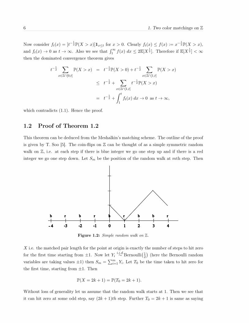


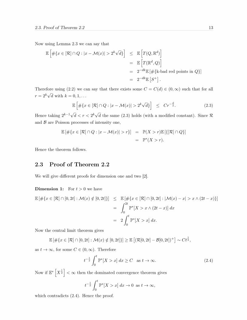


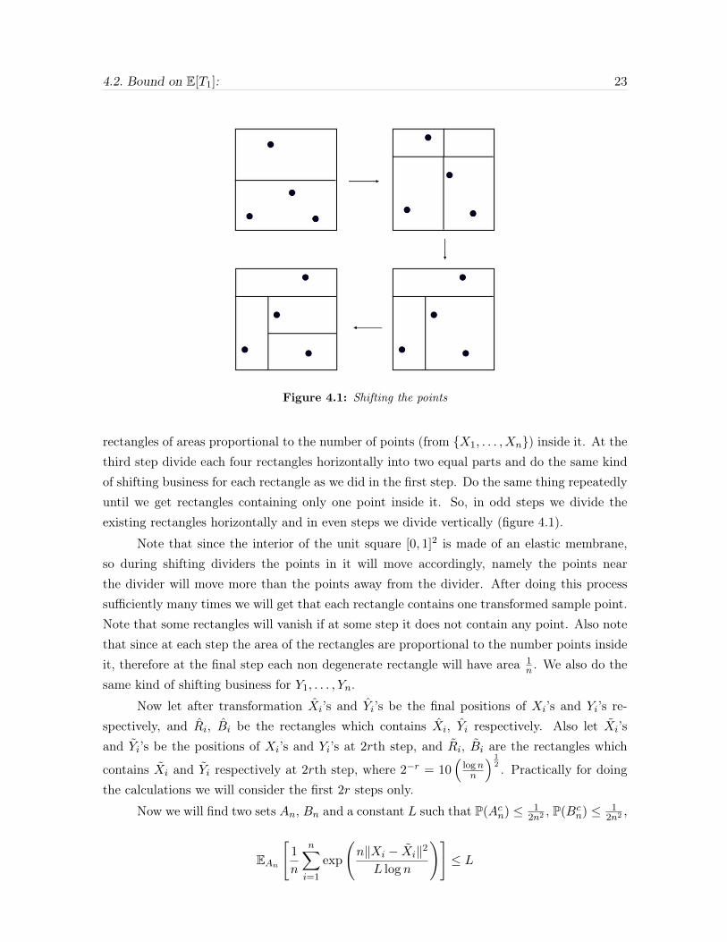


![Analysis of Stable Matchings in R: Package matchingMarkets · Analysis of Stable Matchings in R: ... 4 Analysis of Stable Matchings in R: Package matchingMarkets ... G = 1[V G 0]](https://static.documents.pub/doc/80x56/5b3cc11f7f8b9a9a098b5ae0/analysis-of-stable-matchings-in-r-package-matchingmarkets-analysis-of-stable.jpg)
![Going totally Bananas - Uni Koblenz-Landaulaemmel/120927-delft.pdf · mapM :: Monad m => (a -> m b) -> [a] -> m [b] mapM g = foldr f k where k = return [] f x mys = do](https://static.documents.pub/doc/80x56/5fd84acb32789829e346d478/going-totally-bananas-uni-koblenz-landau-laemmel120927-delftpdf-mapm-monad.jpg)


