General rights Copyright and moral rights for the publications made accessible in the public portal are retained by the authors and/or other copyright owners and it is a condition of accessing publications that users recognise and abide by the legal requirements associated with these rights. Users may download and print one copy of any publication from the public portal for the purpose of private study or research. You may not further distribute the material or use it for any profit-making activity or commercial gain You may freely distribute the URL identifying the publication in the public portal If you believe that this document breaches copyright please contact us providing details, and we will remove access to the work immediately and investigate your claim. Downloaded from orbit.dtu.dk on: Mar 15, 2022 Mean gust shapes Larsen, Gunner Chr. Publication date: 2003 Document Version Publisher's PDF, also known as Version of record Link back to DTU Orbit Citation (APA): Larsen, G. C. (2003). Mean gust shapes. Denmark. Forskningscenter Risoe. Risoe-R No. 1133(EN)
Transcript
General rights Copyright and moral rights for the publications made accessible in the public portal are retained by the authors and/or other copyright owners and it is a condition of accessing publications that users recognise and abide by the legal requirements associated with these rights.
Users may download and print one copy of any publication from the public portal for the purpose of private study or research.
You may not further distribute the material or use it for any profit-making activity or commercial gain
You may freely distribute the URL identifying the publication in the public portal If you believe that this document breaches copyright please contact us providing details, and we will remove access to the work immediately and investigate your claim.
Downloaded from orbit.dtu.dk on: Mar 15, 2022
Mean gust shapes
Larsen, Gunner Chr.
Publication date:2003
Document VersionPublisher's PDF, also known as Version of record
Link back to DTU Orbit
Citation (APA):Larsen, G. C. (2003). Mean gust shapes. Denmark. Forskningscenter Risoe. Risoe-R No. 1133(EN)
Gunner Chr. Larsen, Wim Bierbooms and Kurt S. Hansen Risø National Laboratory, Roskilde, Denmark December 2003
Abstract The gust events described in the IEC-standard are formulated as coherent gusts of an inherent deterministic character, whereas the gusts experienced in real situation are of a stochastic nature with a limited spatial extension. This conceptual difference may cause substantial differences in the load patterns of a wind turbine when a gust event is imposed. Methods exist to embed a gust of a prescribed appearance in a stochastic wind field. The present report deals with a method to derive realistic gust shapes based only on a few stochastic features of the relevant turbulence field. The investigation is limited to investigation of the longitudinal turbulence component, and consequently no attention is paid to wind direction gusts. A theoretical expression, based on level crossing statistics, is proposed for the description of a mean wind speed gust shape. The description also allow for information on the spatial structure of the wind speed gust and rely only on conventional wind field parameters. The theoretical expression is verified by comparison with simulated wind fields as well as with measured wind fields covering a broad range of mean wind speed situations and terrain conditions. The work reported makes part of the project “Modelling of Extreme Gusts for Design Calculations ” (NEWGUST), which is co-funded through JOULEIII on contract no. JOR3-CT98-0239. ISBN 87-550-2587-0 ISBN 87-550-2588-9 (Internet) ISSN 0106-2840 Print: Pitney Bowes management Services Denmark A/S, 2003
Contents
1. BACKGROUND 5
2. INTRODUCTION 6
3. DETERMINATION OF MEAN GUST SHAPE 7
3.1 Theory 7 3.1.1 One point mean gust shape 7 3.1.2 Spatial gust shape 10
4.1 Simulated wind speed time series 17 4.1.1 Wind simulations 17 4.1.2 One point mean gust shape 18 4.1.3 Statistical considerations 19 4.1.4 Spatial gust shape 22 4.1.5 Influence of the sample frequency 24
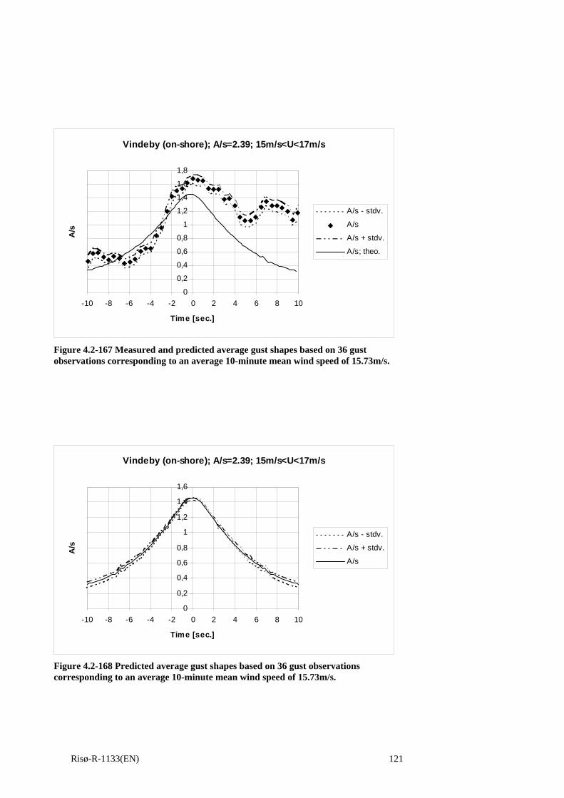
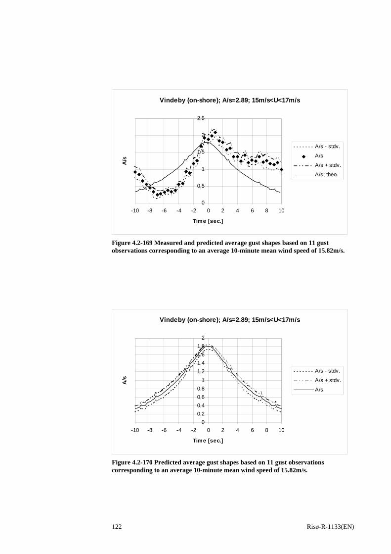
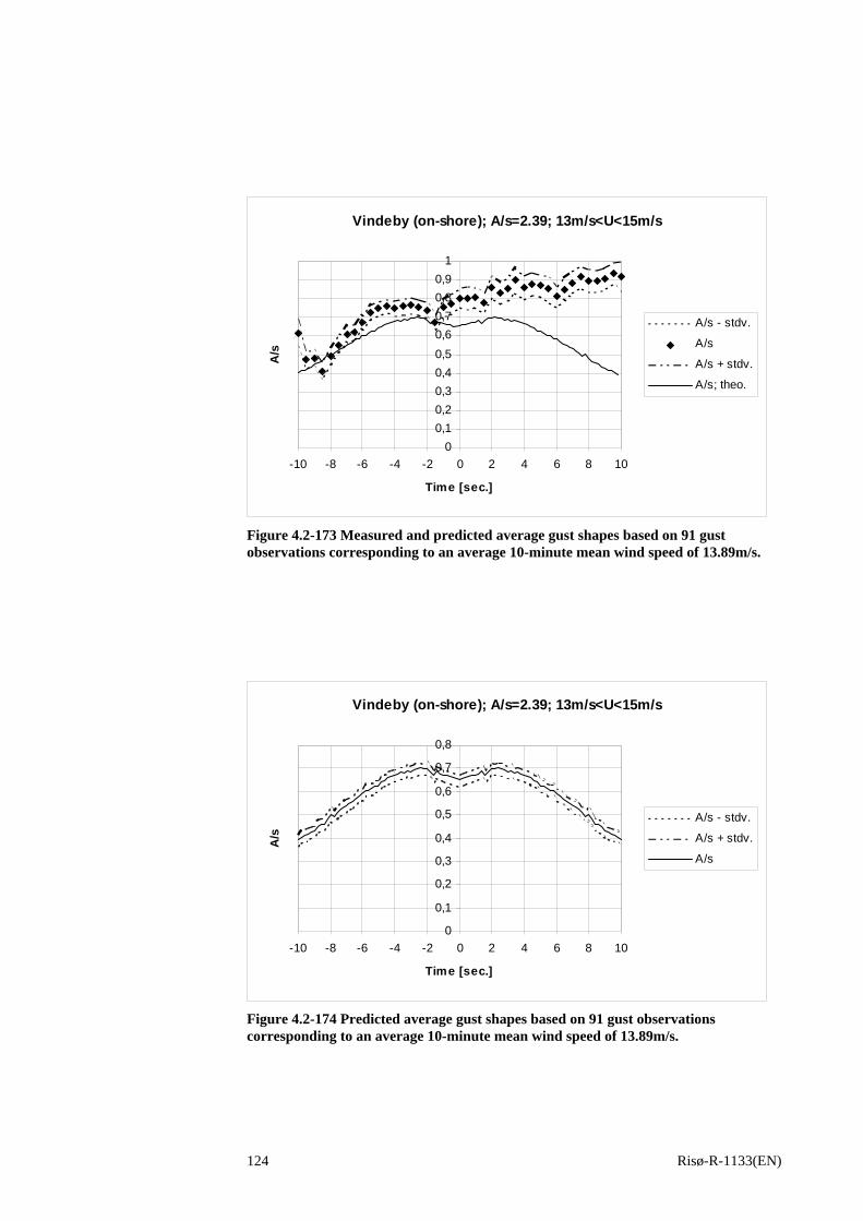
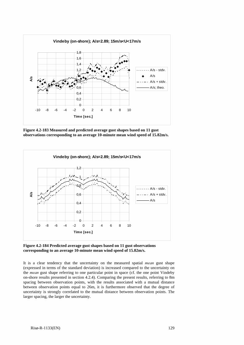
4.2 Wind field measurements 25 4.2.1 Data material 25 4.2.2 Atmospheric stability 30 4.2.3 Gaussian assumption 36 4.2.4 One point mean gust shape 41 4.2.5 Spatial gust shape 108
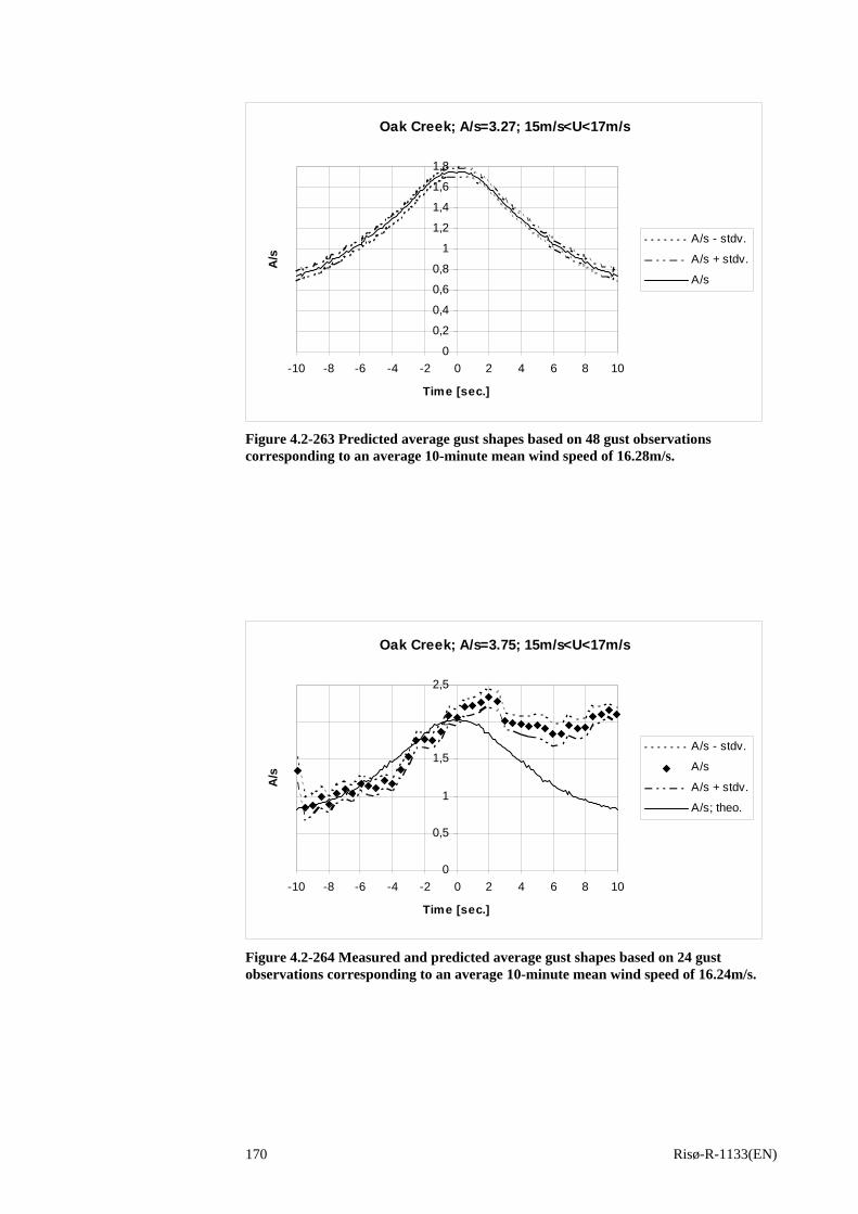
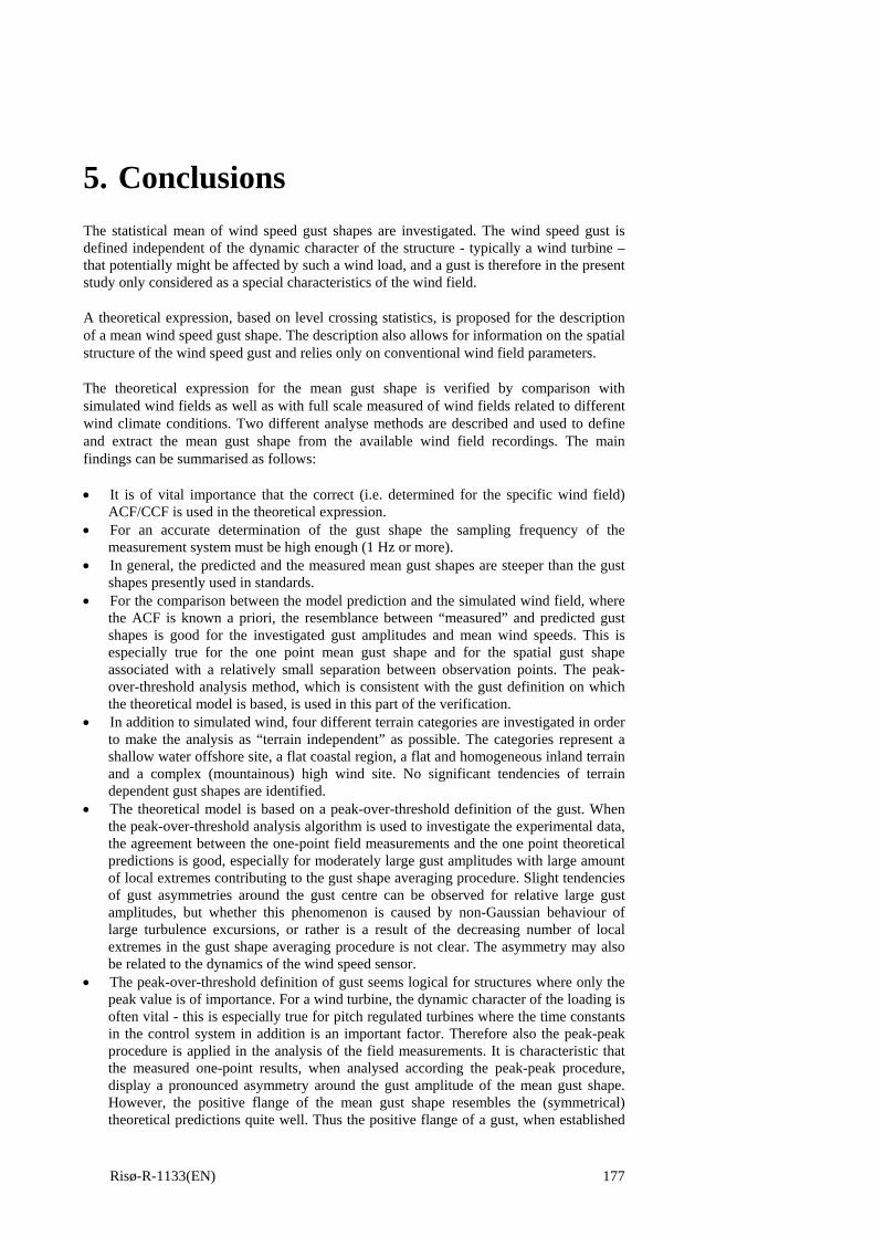
5. CONCLUSIONS 177
6. REFERENCES 179
APPENDIX A 179 APPENDIX B 187 APPENDIX C 189
Risø-R-1133(EN) 3
Risø-R-1133(EN) 4
1. Background The work reported makes part of the project “Modelling of Extreme Gusts for Design Calculations ” (NewGust), which is co-funded through JOULEIII. In essence the NewGust method, describes a way to combine a stochastic turbulence field (as presently used for fatigue analysis) and a well defined deterministic gust shape (which can be theoretically derived) in such a way that a realistic extreme gust is obtained. The project approach can be divided into the following steps: 1) Experimental verification of the shape of extreme gusts. From theory it follows that the
gust shape resembles the autocorrelation function of turbulence. This will be verified by comparing with shapes extracted from an existing database of wind measurements.
2) Determination of the probability distribution function of extreme gusts from a database of wind measurements and/or from theory (in case wind measurements are not available for a long enough period).
3) Development of an advanced method to determine the dynamic response of a wind turbine to extreme gusts. The advanced method will generate wind time series, which can not, in a statistical sense, be distinguished from natural extreme wind gusts.
4) Implementation of the advanced method in a number of existing design packages. 5) Experimental verification of the predicted loading and response of a wind turbine to
extreme gusts. The present report deals with the first of the above described tasks.
Risø-R-1133(EN) 5
2. Introduction The verification of the structural integrity of a wind turbine structure involves analyses of fatigue loading as well as extreme loading arising from the environmental wind climate. With the trend of persistently growing turbines, the extreme loading seems to become relatively more important. The extreme loading to be assessed in an ultimate limit state analyses may result from a number of extreme load events including transient operation (start/stop sequences), faults, and extreme wind events. Examples of extreme wind events are extreme mean wind speeds with a recurrence period of 50 years, extreme wind shear, extreme wind speed gusts and extreme wind direction gusts. The present study addresses extreme wind turbine loading arising only from extreme wind gust events. The extreme wind events explicitly accentuated above are included in the currently available draft of the IEC-standard (IEC 61400-1, 1998) as extreme load conditions that must be considered as ultimate load cases when designing a wind turbine. Within the framework of the IEC-standard, these load situations are defined in terms of two independent site variables - a reference mean wind speed and a characteristic turbulence intensity. However, the gust events described in the IEC-standard are formulated as coherent gusts of an inherent deterministic character, whereas the gusts experienced in real situation are of a stochastic nature with a limited spatial extension. This conceptual difference may cause substantial differences in the load patterns of a wind turbine when a gust event is imposed (Dragt, 1996). In order to introduce more realistic load situations of a stochastic nature, the NewGust project has been launched. The aim of this project is to obtain experimentally verified theoretical methods that allow for embedding (qualified) predefined gusts (with a well described probability of occurrence) in the stochastic of the turbulence atmospheric wind field. This is in line with what is the common practice when dealing with the fatigue loading. The investigation is limited to investigation of the longitudinal turbulence component, and consequently no attention is paid to wind direction gusts. The present report deals with the description of the average gust shape. A theoretical expression, based on level crossing statistics, is proposed for the description of a mean wind speed gust shape. The description also allows for information on the spatial structure of the wind speed gust and relies only on conventional wind field parameters. The theoretical expression is verified by comparison with simulated wind fields as well as with measured wind fields covering a broad range of wind speed situations, atmospheric stability situations and terrain conditions.
Risø-R-1133(EN) 6
3. Determination of mean gust shape
3.1 Theory A theoretical expression for a mean gust shape has been derived at Delft University based on a general method to determine statistical means of certain parameters of a stationary stochastic process. The method is due to Middleton (Middleton, 1960). Both one point mean gust shapes - i.e. gust shapes at the particular spatial point where the gust is defined - and the spatial extension of a mean gust shape has been investigated.
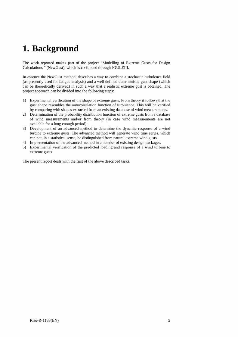
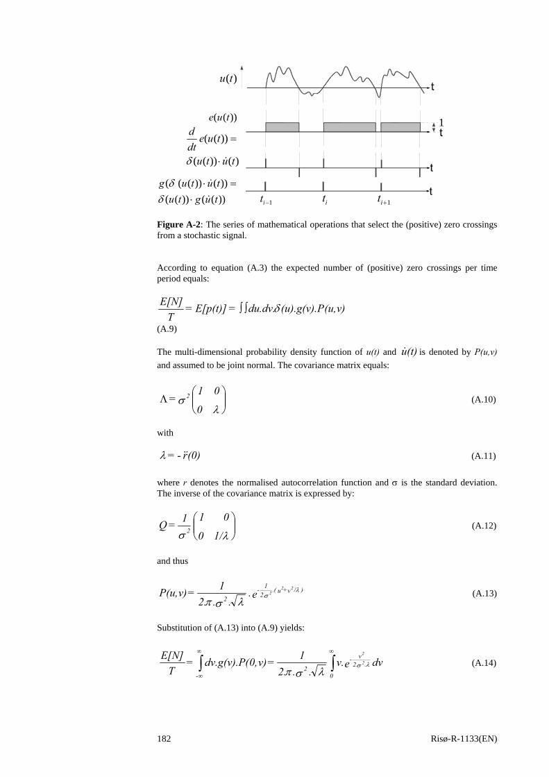
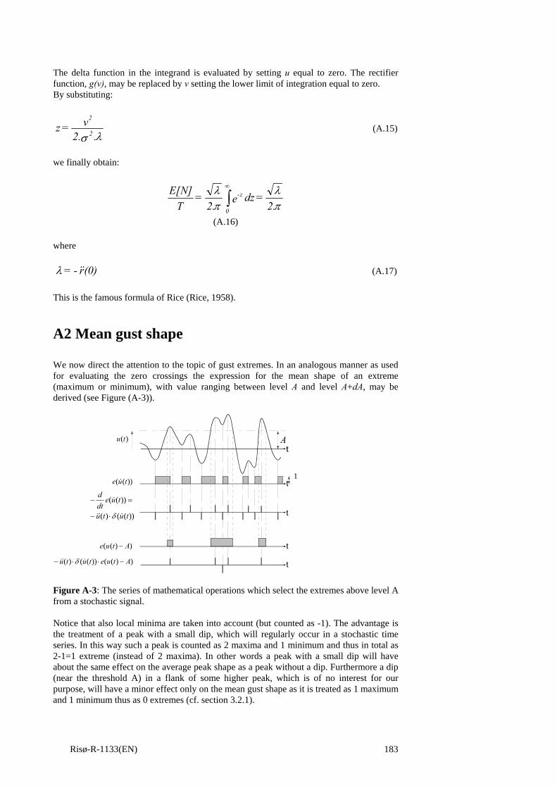
3.1.1 One point mean gust shape The Delft model is based on an assumption of Gaussian turbulence and a peak over threshold definition of a gust. Based on these assumptions an analytical expression for the mean gust shape can be determined depending only on basic statistical quantities related to the turbulence time series. A full treatment of the analytical derivation of this expression is given in Appendix A. The derivation is based on a general method (Middleton, 1960) for the determination of a mean quantity associated with a stationary stochastic process. This method essentially consists of two steps. In the first step (mathematical) operations must be determined which has the ability of transforming the original stochastic wind speed signal into a time series consisting of delta functions positioned at the time instants corresponding to specified events - in our case the local extremes. This is illustrated in Figure (3.1-1).
)(tu
))(( tue
))(( Atue −
))(())(()( Atuetutu −⋅⋅− δ
))(()(
))((
tutu
tuedtd
δ⋅−
=−
A
1
Figure 3.1-1 The mathematical operations which defines extremes above a threshold, A, from a stochastic signal.
The mean gust shape can be expressed as a multi-dimensional integral of an integrand involving the last expression given on Figure (3.1-1) and a multi-dimensional probability density function.
Risø-R-1133(EN) 7
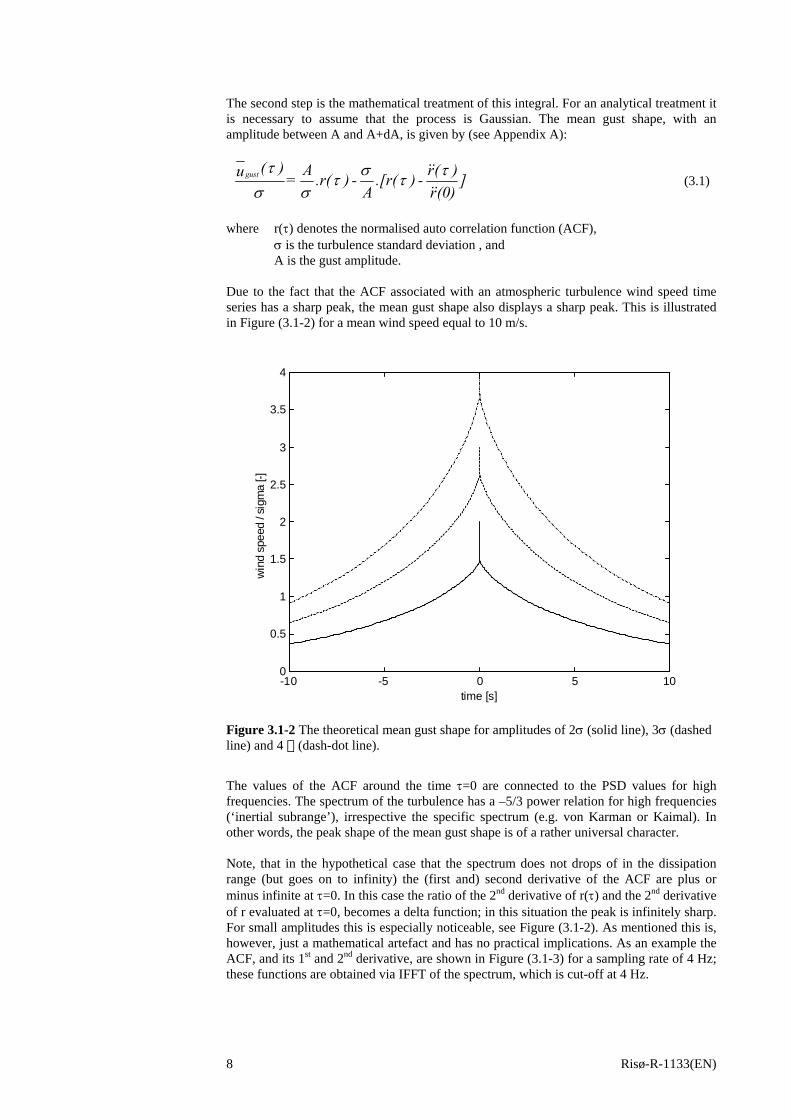
The second step is the mathematical treatment of this integral. For an analytical treatment it is necessary to assume that the process is Gaussian. The mean gust shape, with an amplitude between A and A+dA, is given by (see Appendix A):
](0)r
)(r-).[r(A
-).r(A = )(ugust ττστ
σστ
(3.1)
where r(τ) denotes the normalised auto correlation function (ACF),
σ is the turbulence standard deviation , and A is the gust amplitude. Due to the fact that the ACF associated with an atmospheric turbulence wind speed time series has a sharp peak, the mean gust shape also displays a sharp peak. This is illustrated in Figure (3.1-2) for a mean wind speed equal to 10 m/s.
-10 -5 0 5 100
0.5
1
1.5
2
2.5
3
3.5
4
win
d sp
eed
/ sig
ma
[-]
time [s]
Figure 3.1-2 The theoretical mean gust shape for amplitudes of 2σ (solid line), 3σ (dashed line) and 4 (dash-dot line).
The values of the ACF around the time τ=0 are connected to the PSD values for high frequencies. The spectrum of the turbulence has a –5/3 power relation for high frequencies (‘inertial subrange’), irrespective the specific spectrum (e.g. von Karman or Kaimal). In other words, the peak shape of the mean gust shape is of a rather universal character. Note, that in the hypothetical case that the spectrum does not drops of in the dissipation range (but goes on to infinity) the (first and) second derivative of the ACF are plus or minus infinite at τ=0. In this case the ratio of the 2nd derivative of r(τ) and the 2nd derivative of r evaluated at τ=0, becomes a delta function; in this situation the peak is infinitely sharp. For small amplitudes this is especially noticeable, see Figure (3.1-2). As mentioned this is, however, just a mathematical artefact and has no practical implications. As an example the ACF, and its 1st and 2nd derivative, are shown in Figure (3.1-3) for a sampling rate of 4 Hz; these functions are obtained via IFFT of the spectrum, which is cut-off at 4 Hz.
Risø-R-1133(EN) 8
-10 -5 0 5 100.2
0.3
0.4
0.5
0.6
0.7
0.8
0.9
1
-10 -5 0 5 10-0.2
-0.15
-0.1
-0.05
0
0.05
0.1
0.15
0.2
-10 -5 0 5 10-6
-5
-4
-3
-2
-1
0
1
Figure 3.1-3 The ACF and its first and second derivative; for a sampling rate of 4 Hz.
For the extreme wind turbine loading, gusts with large amplitudes are of primary interest. In that case the first term in equation (3.1) is dominating; and the gust shape thus basically resembles the ACF. This is in agreement with the expression (for large amplitudes) due to Lindgren (Lindgren, 1970), which is based on analyses of local maxima only. This expression has been used in a method to determine the extreme hydrodynamic wave loading for offshore platforms (Taylor, 1997). The effect from the mean wind speed on the gust shape is illustrated in Figure (3.1-4). The figure demonstrates the necessity to distinguish gusts from different mean wind speeds. An alternative to mean wind speed binning is to transform the time axis into a distance axis by application of the Taylor frozen turbulence hypothesis.
-10 -5 0 5 100
0.5
1
1.5
2
2.5
3
3.5
4
win
d sp
eed
/ sig
ma
[-]
time [s]
Figure 3.1-4 The theoretical mean gust shape for a mean wind speed of 10 m/s (solid line) and 20 m/s (dashed line).
The dependency of the gust shape on the specific ACF is shown in Figure (3.1-5), where the von Karman ACF is compared to the ACF given in ESDU (ESDU); the formulation in ESDU is equivalent with the von Karman expression except for the length scale. It can be concluded that for verification purposes the correct ACF (i.e. determined for the specific site) should be used in the theoretical expression.
Risø-R-1133(EN) 9
-10 -5 0 5 100.5
1
1.5
2
2.5
3
3.5
4
win
d sp
eed
/ sig
ma
[-]
time [s]
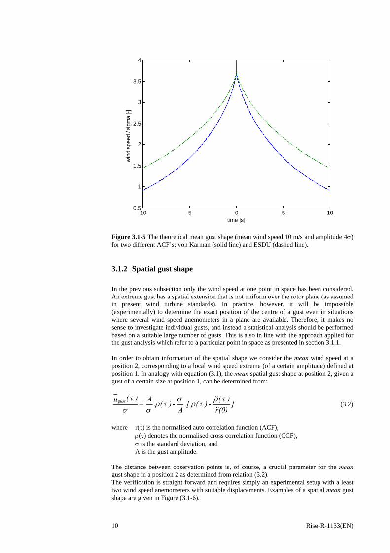
Figure 3.1-5 The theoretical mean gust shape (mean wind speed 10 m/s and amplitude 4σ) for two different ACF’s: von Karman (solid line) and ESDU (dashed line).
3.1.2 Spatial gust shape In the previous subsection only the wind speed at one point in space has been considered. An extreme gust has a spatial extension that is not uniform over the rotor plane (as assumed in present wind turbine standards). In practice, however, it will be impossible (experimentally) to determine the exact position of the centre of a gust even in situations where several wind speed anemometers in a plane are available. Therefore, it makes no sense to investigate individual gusts, and instead a statistical analysis should be performed based on a suitable large number of gusts. This is also in line with the approach applied for the gust analysis which refer to a particular point in space as presented in section 3.1.1. In order to obtain information of the spatial shape we consider the mean wind speed at a position 2, corresponding to a local wind speed extreme (of a certain amplitude) defined at position 1. In analogy with equation (3.1), the mean spatial gust shape at position 2, given a gust of a certain size at position 1, can be determined from:
](0)r
)(-)(.[A
-)(.A = )(ugust τρτρστρ
σστ
(3.2)
where r(τ) is the normalised auto correlation function (ACF),
ρ(τ) denotes the normalised cross correlation function (CCF), σ is the standard deviation, and
A is the gust amplitude. The distance between observation points is, of course, a crucial parameter for the mean gust shape in a position 2 as determined from relation (3.2). The verification is straight forward and requires simply an experimental setup with a least two wind speed anemometers with suitable displacements. Examples of a spatial mean gust shape are given in Figure (3.1-6).
Risø-R-1133(EN) 10
-10 -5 0 5 100
0.5
1
1.5
2
2.5
3
3.5w
ind
spee
d / s
igm
a [-]
time [s]
Figure 3.1-6 The theoretical mean spatial gust shape; for an amplitude of 4σ. The upper curves correspond with a distance of 5 m, V=10 m/s (solid line) and V=20 m/s (dash-dot line); the lower curves with a distance of 40 m, V=10 m/s (dashed line) and V=20 m/s (dotted line).
-10 -5 0 5 100.6
0.8
1
1.2
1.4
1.6
1.8
2
win
d sp
eed
/ sig
ma
[-]
time [s]
Figure 3.1-7 The theoretical mean gust shape at position 2 (mean wind speed 10 m/s, distance 40 m and amplitude 4σ at position 1) for two different ACF: von Karman (solid line) and ESDU (dashed line).
Figure (3.1-7) illustrates the large influence of the CCF on the spatial gust shape. The same conclusion can be drawn as for the mean gust shape defined with reference to only one
Risø-R-1133(EN) 11
point in space; for verification purposes the CCF of the specific site should be applied in the theoretical expression.
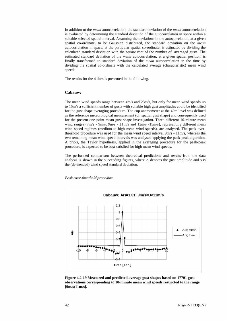
3.2 Experiments The present section deals with analyse methods to define and extract mean gust shapes from a stochastic wind field. The wind field observations may originate from field measurements or from computer simulations. Such analysis methods are required for verification of theoretical predicted mean gust shapes. Initially, a procedure for identifying individual gusts in a stochastic wind time series is required. Subsequently a suitable averaging procedure must be defined. Several possibilities exist. One possibility is to consider a gust as the part of a particular signal between a positive and a succeeding negative level crossing. However, usually several local extremes will occur in the time interval defined by the two associated level crossings for a broad banded stochastic signal such as the atmospheric turbulence, the occurrence of several local maxima complicates the definition of an associated gust amplitude. Another possibility is simply to interpret a gust as the signal extending in a certain (arbitrary) selected time interval around a local extreme (of a prescribed size). The mean gust shape, conditioned on amplitude size, is consequently obtained from weighted averaging of all wind speed time series around the localised extremes. A third possibility is to define a time “window” of a suitable length comparable with the time extend of the gust type of particular relevance. Moving the “window” along the time axis, a gust is defined every time a suitable (predefined) large wind speed excursion between a local minimum and a local maximum inside the window is identified. To separate gusts only the largest event, within a time interval corresponding to the time integral scale of the process, is accepted. In the present investigation the second and the third procedure has been applied. The second method will in the following be denoted the “Peak-Over-Threshold Procedure” whereas the third method will be denoted the “Peak-Peak Procedure”.
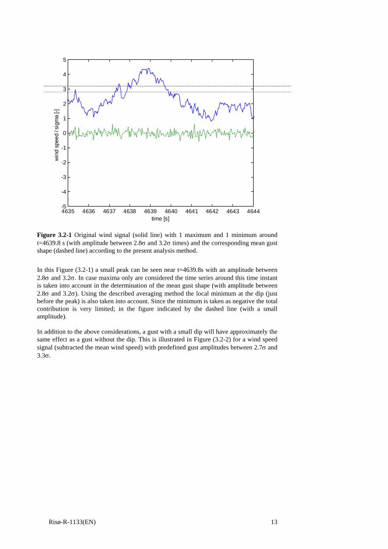
3.2.1 Peak-Over-Threshold Procedure According to this algorithm, a gust is interpreted as an arbitrary selected time period around a local extreme of a predefined size in the wind speed time series. The gust amplitude, measured as the excursion from the mean wind speed is often measured in terms of standard deviation of the particular wind speed time series (denoted by in the following). The mean gust shape, with a given amplitude, follows by straightforward weighted averaging of the pieces of the wind time series around all found extremes. In the averaging procedure a (local) maximum is assigned the weight +1 whereas a (local) minimum is assigned the weight -1. The weighted averaging procedure is adopted at the expense of an averaging procedure, which only takes the local maxima into account, to avoid significant contributions from local disturbances on a flank of a major peek, and is as such an analogy to the definition of a gust as a part of a particular signal between a positive and a succeeding negative level crossing. This is illustrated in Figure (3.2-1) for a wind speed signal (subtracted the mean wind speed) with predefined gust amplitudes, A, between 2.8σ and 3.2σ.
Figure 3.2-1 Original wind signal (solid line) with 1 maximum and 1 minimum around t=4639.8 s (with amplitude between 2.8σ and 3.2σ times) and the corresponding mean gust shape (dashed line) according to the present analysis method.
In this Figure (3.2-1) a small peak can be seen near t=4639.8s with an amplitude between 2.8σ and 3.2σ. In case maxima only are considered the time series around this time instant is taken into account in the determination of the mean gust shape (with amplitude between 2.8σ and 3.2σ). Using the described averaging method the local minimum at the dip (just before the peak) is also taken into account. Since the minimum is taken as negative the total contribution is very limited; in the figure indicated by the dashed line (with a small amplitude). In addition to the above considerations, a gust with a small dip will have approximately the same effect as a gust without the dip. This is illustrated in Figure (3.2-2) for a wind speed signal (subtracted the mean wind speed) with predefined gust amplitudes between 2.7σ and 3.3σ.
Risø-R-1133(EN) 13
5944.5 5945 5945.5 5946 5946.5 59470.5
1
1.5
2
2.5
3
3.5
win
d sp
eed
/ sig
ma
[-]
time [s]
A/sigma=3.3
A/sigma=2.7
Figure 3.2-2 Original wind speed signal (solid line) with 2 maxima and 1 minimum around t=5945.5 s (with amplitude between 2.7σ and 3.2σ) and the corresponding mean gust shape (dashed line) according to the present analysis method.
Note, that a gust with the above character will have a twice as large influence on the mean gust shape as a gust without a small dip, in case local maxima only are considered. The illustrated procedure can be summarised as follows: • Normalise the wind speed time series by subtracting its mean value and by division by
its standard deviation. • Search in the wind speed time series for local extremes; thus either local maxima or
local minima (thus no condition on the second derivative). The local maxima are found from a change of the first derivative from positive to negative; and vice versa for the local minima.
• Select the gusts with the desired gust amplitude; e.g. between 1.5σ and 2.5σ. • Extract pieces of the wind time series around the found extremes; e.g. 10 s before and
10 s after the extreme. • Perform a weighted average of all found pieces with weight equal to +1 and -1 for
local maxima and minima, respectively. In other words, the gust shape around a maximum (minimum) is added to (subtracted from) the sum of gust shapes and the total number of gusts is increased (decreased) by 1.
To obtain a robust estimate of the mean gust shape, a suitable number of gusts must be identified - usually of the order of magnitude 50 or more. The above outlined algorithm deals with wind speed gusts as observed at a specific point in space. In order to obtain information of the spatial shape of the mean wind speed gust an analogue procedure can be applied. In the present context the wind speed at a position 2, corresponding to a local wind speed extreme at position 1, yield information of the spatial mean gust shape. The analysis procedure is equivalent to the one-point procedure: • Normalise the wind speed time series at the two positions by subtracting the mean
value (for each position) and by division by the standard deviation (for each position).
Risø-R-1133(EN) 14
• Search in the wind time series at position 1 for time instants of local extremes; thus either local maxima or local minima (thus no condition on the second derivative). The local maxima are found from a change of the first derivative from positive to negative; and vice versa for the local minima.
• Define the gusts from the time series at position 1 with a predefined gust amplitude; e.g. between 1.5σ and 2.5σ.
• Extract the pieces of the wind speed time series at position 2 around the time instant of the extremes found in the time series for position 1; e.g. 10 s before until 10 s after the extreme.
• Perform a weighted average of all found pieces referring to position 2 with weight equal to +1 and -1 for local maxima and minima, respectively. In other words, the gust shape around a maximum (minimum) is added to (subtracted from) the sum of gust shapes and the total number of gusts is increased (decreased) by 1.
Note, that the peak-over-threshold analysis method implicitly assumes stationary time series and that consequently trends, if present, must be removed to obtain consistent results.
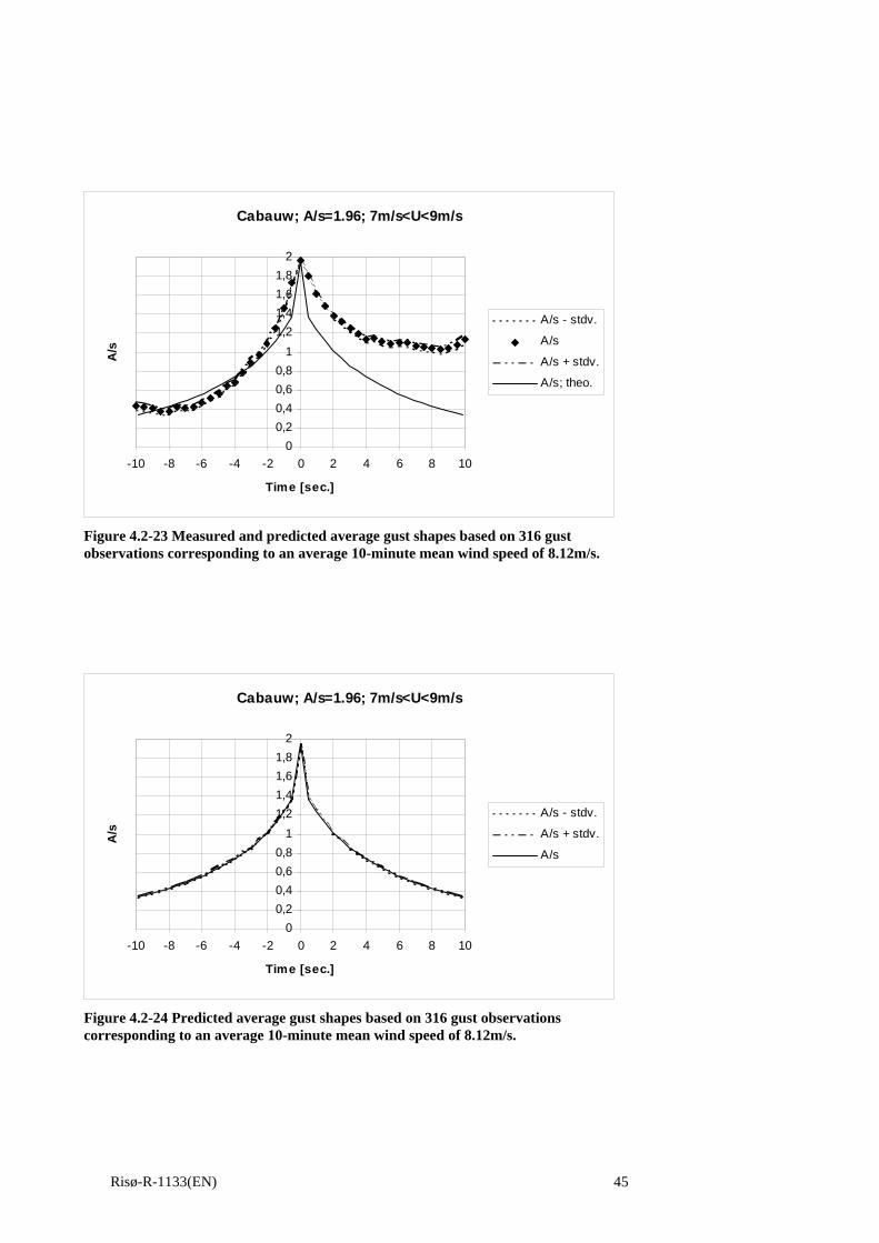
3.2.2 Peak-Peak Procedure The peak-peak procedure is based on a window technique. Initially, a time window of a suitable time length, comparable with the time extend of the gust type of particular relevance, is defined. The time extend of the considered window may be determined based on considerations of the wind turbines dynamically properties, time constants related to the control system etc.. Moving the “window” along the time axis with time increments corresponding to the sample frequency of the wind speed signal, a gust is defined every time a suitable (predefined) large wind speed excursion between a local minimum and a local maximum inside the window is identified. This wind speed excursion will in the following be referred to as the gust amplitude. To separate individual gusts only the largest event, within a time interval corresponding to the time integral scale of the process, is accepted. Before applying the window procedure to a time series a de-trending is performed. The theoretical gust shape is based on an assumption of stationary “parent“ stochastic processes, and in order to obtain a consistent comparison with experimental time series, it is necessary to remove possible trends in these. This is especially important as correlation functions are known to be particularly sensitive to low frequency errors (Panofsky, 1983). Obviously, also standard deviations are sensitive to trends in the time series. There is no standard technique to perform this trend removal, and consequently the resulting correlation functions tend to depend on the method applied. A visual inspection of the time series may provide ideas for a suitable strategy. In the present analysis the widely used linear trend removal is applied. For a given range (bin interval) of gust amplitudes, the mean gust shape, associated with this bin class, is obtained from an averaging procedure. For each identified gust situation, the time signal extending in a certain selected time interval around the gust peak is extracted. The selected time intervals must have an extend that ensures that the transformations (to be described in the following) from a time scale to a spatial scale and back to a weighted time scale results in the desired size the resulting time interval. Assuming Taylor’s frozen turbulence hypothesis to be valid, the (frozen) turbulence is presumed convected in the mean wind direction with the mean wind speed. The hypothesis thus enables us to convert temporal measurements at a given point in space to spatial patterns in space. In real life the turbulence is neither frozen, nor convected with the mean wind speed. However, for eddy-passing times small compared to the eddy life times (high winds and moderate shear) it is common practice to consider the turbulence to satisfy the hypothesis quite well. In the present averaging procedure the Taylor hypothesis is assumed valid. This is considered justified by the fact that ultimate gust loading is closely correlated with high mean wind speeds.
Risø-R-1133(EN) 15
The selected time intervals around identified gusts are subsequently transformed from a time scale to a spatial scale by multiplication with the particular mean wind speeds (corresponding to the stationary time series) in accordance with the Taylor hypothesis. In general, time series corresponding to a particular site are sampled with a constant sample rate. In order to obtain a comparable resolution in the length scale for gusts to be averaged a binning in the mean wind speed is applied. A bin size of 2m/s was found suitable. Having transformed gusts, belonging to a given gust amplitude and given mean wind speed bin class, to the spatial scale, these are subsequently centred on the gust peak and averaged straightforward. The weighted average of the mean wind speeds (corresponding to the stationary time series) is now determined with weights equating the number of gust occurrences within a given stationary wind speed time series. In the present analysis all stationary wind speed time series are 10-minute time series. Finally, the averaged mean wind speed is used to transform the spatial mean gust shape into a time mean gust shape referring to this distinct mean wind speed. In addition to the mean gust shape, the standard deviation of the mean gust shape is evaluated by determining the standard deviation of the gust shape within a suitable spatial interval. Assuming the deviations in the gust shape at a given spatial co-ordinate to be Gaussian distributed, the standard deviation on the mean gust shape, at the particular spatial co-ordinate, is obtained by dividing the calculated standard deviation with the square root of the number of averaged gusts. The estimated standard deviation of the mean gust shape at a given spatial position is finally transformed to standard deviation of the mean gust shape in the time domain by dividing the spatial co-ordinate with the calculated average mean wind speed. The peak-peak algorithm, as outlined above, deals with wind speed gusts observed at a specific point in space. However, in order to obtain information of the spatial shape of the mean wind speed gust an similar procedure can be applied. In analogy with the peak-over-threshold algorithm the wind speed at a position 2, corresponding to a local wind speed extreme at position 1, yield information of the spatial mean gust shape. The analysis procedure is in this situation as follows: • Identify a number of gusts of a predefined size from de-trended wind speed time
series, associated with measurement position 1, applying the window algorithm described above.
• Extract pieces of the wind speed time series at position 2 around the time instant of the identified gusts associated with the wind speed time series for position 1.
• The extracted time series intervals, related to position 2, are subsequently transformed from a time scale to a spatial scale by multiplication with the particular mean wind speeds at position 2 in accordance with the Taylor hypothesis. To obtain a reasonably uniform spatial resolution mean wind speed binning has been applied, and mean wind speed bins of 2m/s was found suitable.
• The mean shape at position 2, belonging to a given gust amplitude at position 1 and a given mean wind speed bin class, is then obtained by centring the extracted wind speed series, associated with position 2, around the centre of the spatial intervals (obtained from the transformation) and subsequently averaging straight forward.
• The weighted average of the mean wind speeds at position 2, using the weights defined in the one point gust analysis, is evaluated and finally used to transform the spatial mean gust shape at position 2 into a time mean gust shape at position 2.
In analogy with the one-point investigation, standard deviations on the computed mean gust shapes can be evaluated. The procedure is equivalent to the procedure described for the one-point analysis.
Risø-R-1133(EN) 16
4. Verification of mean gust shape The present chapter deals with a verification of the theoretical model for the mean gust shape presented in section 3.1. The verification is performed by comparing model predictions to both wind simulations and (full scale) wind field measurements. The verification using simulated wind speed time series has the advantage that the autocorrelation function and cross correlation functions, required in the theoretical predictions, are known a priori as input to the wind field generator. In case a von Karman spectrum is selected as a target spectrum, analytical expressions exist for these quantities. For the verification based on field measurements, the required autocorrelation and cross correlation functions must be estimated based on the measured wind speed time series. The two methods, described in details in sections 3.2.1 and 3.2.2, are applied to identify gusts and evaluate the associated mean gust shape from the investigated data material.
4.1 Simulated wind speed time series For evaluation of the analytical expression for the mean gust shape, the autocorrelation function (ACF) must be known - cf. equation (3.1). This implies that a comparison between the determined mean gust shape, as obtained from field measurements, and the theoretical prediction will be affected by uncertainty in the determination in the ACF. In order to circumvent this problem a verification is conducted based on a simulated wind field, where the ACF is known priori as input of the wind field simulation. In addition possible influences on the determined mean gust shape, originating from the measurement system, can easily be studied by computer simulations. The verification of predicted mean gust shapes against mean gust shapes, evaluated from simulated wind speed time series, is conducted using the peak-over-threshold algorithm described in section 3.2.1.
4.1.1 Wind simulations With the aid of the wind field simulation package SWING4 (Bierbooms, 1998), time series are generated for two mean wind speeds (10 m/s and 20 m/s), for heights equal to 35 m, 40 m and 80 m. SWING4 is an acronym for Stochastic WINd Generator. It is capable to generate all three velocity components of wind turbulence. A special feature of SWING4 is that the wind velocities are calculated only at the desired points on the (rotating) blades instead of at some fixed points in the rotor plane. SWING4 is fully compatible with the commonly applied standards for wind turbine design: IEC, GL and Danish Standard. SWING4 is based on the energy spectrum of von Karman in combination with the commonly applied Taylor’s frozen turbulence hypothesis. This corresponds to the von Karman isotropic turbulence model as given in the IEC standard for wind turbine load calculations (Draft IEC, 1998). The application of the energy spectrum of von Karman implies that implicitly all coherences (thus Cuu, Cvv, Cww, Cuv, Cuw and Cvw, where u denotes the longitudinal, v the lateral and w the vertical velocity component) are included in a consistent way. This can not be achieved applying other theoretical or measured spectra and coherence functions. Although SWING4 is based on the isotropic turbulence theory, the method is adopted in such a way that alternative spectra (from theory or from measurements) can be used (e.g. the spectra given in the IEC and Danish Standard). For our purpose the longitudinal component of the generated wind field only will be used. The isotropic turbulence model has been chosen: the von Karman spectrum and the corresponding coherency functions, which may be expressed in modified Bessel functions of the 2nd kind (cf. Appendix C). In order to obtain the stochastic wind field in a fixed reference of frame, the rotational speed (of a hypothetical wind turbine) has been set to a
Risø-R-1133(EN) 17
very low value. The generated wind fields have been extensively tested to produce the required spectra. In order to generate a sufficient amount of gusts, 100 wind field realisations have been generated for each investigated mean wind speed - each of a duration of more than 10 minutes and with a relative high sampling rate (16384 time steps of 0.04 s).
4.1.2 One point mean gust shape In Figure (4.1-1) the mean gust shapes, for a mean wind speed of 10 m/s and for two different gust amplitudes, are given according to the theoretical expression (3.1) and compared with the mean shapes determined from the simulated wind speed time series. As it can be seen the resemblance is good. The small deviations are due to the stochastic nature of turbulence.
-10 -5 0 5 100
0.5
1
1.5
2
2.5
3
win
d sp
eed
/ sig
ma
[-]
time [s]-10 -5 0 5 100
0.5
1
1.5
2
2.5
3
3.5
4
win
d sp
eed
/ sig
ma
[-]
time [s] Figure 4.1-1 Mean gust shapes predicted from the theory (solid lines) and extracted from the simulated wind data (dashed lines) for a mean wind speed equal to 10 m/s. a) Gust amplitude 3σ (479 gusts). b) Gust amplitude 4σ (26 gusts). The mean gust shapes, obtained for the mean wind speeds 10m/s and 20 m/s, are presented in Figure (4.1-2) for gust amplitudes equal to 3σ. For each mean wind speed the theoretically predicted mean gust shape is compared to the mean gust shapes extracted from the simulated wind speed records. The mean gust shapes, as evaluated from the simulated wind speed records, is based on 479 gusts for the 10m/s situation and on 541 gusts for the 20m/s situation.
Risø-R-1133(EN) 18
-10 -5 0 5 100
0.5
1
1.5
2
2.5
3
win
d sp
eed
/ sig
ma
[-]
time [s]
Figure 4.1-2 The comparison of mean gust shapes predicted from theory (solid lines) and determined from simulated wind (dashed lines), for a gust amplitude equal to 3σ and mean wind speeds 10 m/s (upper curves; 479 gusts) and 20 m/s (lower curves; 541 gusts), respectively.
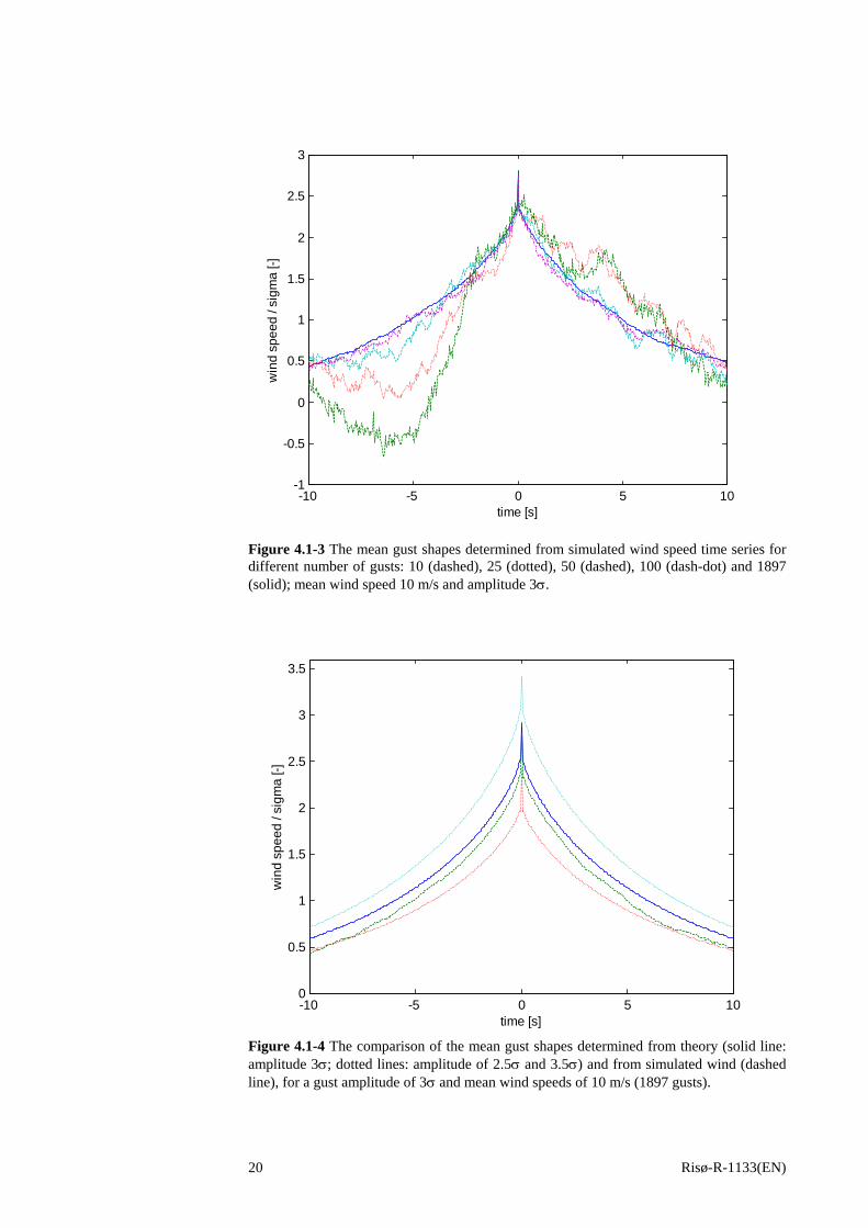
4.1.3 Statistical considerations In this subsection considerations on the statistical significance of the obtained mean gust shapes are presented. The convergence of the mean gust shape are investigated in Figure (4.1-3) where mean gust shapes based on 10, 25, 50, 100 and 1897 gust observations have been compared. The identified gusts refer to a mean wind speed equal to 10m/s and a gust amplitude equal to 3σ. Based on a visual inspection of the results, it may be concluded that of the order of magnitude 50 gusts (or more) are needed to obtain a sufficient convergence in the mean gust shape. Note, however, that the investigation is restricted to only one mean wind speed and only one gust amplitude and is performed only for the peak-over-threshold gust averaging procedure, which might affect the generality of the result.
Risø-R-1133(EN) 19
-10 -5 0 5 10-1
-0.5
0
0.5
1
1.5
2
2.5
3
win
d sp
eed
/ sig
ma
[-]
time [s]
Figure 4.1-3 The mean gust shapes determined from simulated wind speed time series for different number of gusts: 10 (dashed), 25 (dotted), 50 (dashed), 100 (dash-dot) and 1897 (solid); mean wind speed 10 m/s and amplitude 3σ.
Figure 4.1-4 The comparison of the mean gust shapes determined from theory (solid line: amplitude 3σ; dotted lines: amplitude of 2.5σ and 3.5σ) and from simulated wind (dashed line), for a gust amplitude of 3σ and mean wind speeds of 10 m/s (1897 gusts).
-10 -5 0 5 100
0.5
1
1.5
2
2.5
3
3.5
win
d sp
eed
/ sig
ma
[-]
time [s]
Risø-R-1133(EN) 20
An easy way to increase the number of gust realisations in the averaging process is to apply a large gust amplitude bin range in the analysis method. In Figure (4.1-3) an amplitude bin interval ranging between 2.5σ and 3.5σ is applied. The problem with a large gust amplitude range is however that the determined mean gust shape will converge towards too low values. This is due to the fact that the mean of a 2.5σ gust and a 3.5σ gust is not exactly equal to the mean gust shape of a 3σ gust. But more important, gusts with smaller amplitudes will occur more often than larger gusts. This implies that averaging over all gusts will lead to a mean gust shape with a smaller amplitude than 3σ. This is demonstrated in Figure (4.1-4). However, this inexpediency can be accounted for by associating the mean gust shape to a gust amplitude evaluated as mean of all the gust amplitudes contributing in the averaging procedure rather than associating it to a gust amplitude equal to the mean of the gust amplitude range interval. In order to approach the correct convergence, an amplitude range of only 0.3σ have been applied in the Figures (4.1-1) and (4.1-2). The standard error may be considered as a measure of the accuracy of the determined mean gust shape (for each time instant). In case of a Gaussian distribution of the mean gust values for a certain time instant, the standard error is inversely proportional to the square root of the number of gusts. The Gaussian assumption for the distribution of the mean gust values is satisfied in case the number of gusts is large, due to the central limit theorem (independently from the original distribution of the gust values, for a certain time instant). Note that the distribution of the gust values for the time instant t=0 s forms an exception, because all gust centres are moved (along the time axis) to t=0. In case of a Gaussian distribution the values should be lying, with a probability of 95%, within a range of plus and minus 2 times the standard error. This is shown in Figure (4.1-5).
-10 -5 0 5 100
0.5
1
1.5
2
2.5
3
win
d sp
eed
/ sig
ma
[-]
time [s]
Figure 4.1-5 Comparison of the mean gust shapes predicted by the theory (solid line) and obtained from simulated wind (dashed line). The uncertainty range (dotted lines; 2 times the standard error) is also given. Gust amplitude 3σ and mean wind speed 10 m/s (479 gusts).
Risø-R-1133(EN) 21
For large (absolute) time values the agreement between the theoretical shape and based on simulated wind is somewhat less. This is due to the limited end time of the generated time series (approximately 600 s which is standard for meteorological recordings). A consequence of the limited length of the records is that the related frequency step is also finite. In other words, the low frequencies are not so good represented in the time series; this results in the familiar large scatter and too low values for low frequencies in the corresponding power spectrum. A similar effect occurs, for large time values, in the auto (and cross) correlation function. As mentioned previously (cf. section 3.1.1) the expression for the mean gust shape taking all local extremes into account converge for large amplitudes to the expression where only the local maxima is considered. This is illustrated in Figure (4.1-6) where the small difference between the two analysis methods is illustrated for the rather large gust amplitude 4σ. The mean wind speed in the example is 10m/s.
-10 -5 0 5 10
0
0.5
1
1.5
2
2.5
3
3.5
4
win
d sp
eed
/ sig
ma
[-]
time [s]
Figure 4.1-6 Comparison of the mean gust shapes predicted from theory (solid line) and from simulated wind. The dashed line (115 gusts) represents the analysis taking into account all local extremes, whereas the dash-dotted line (164 gusts) represents an analysis where only the local maxima is considered. The difference between the results from the two analysis methods is represented by the solid line around zero.
4.1.4 Spatial gust shape This section deals with the spatial gust shape. For this purpose the generated wind time series at different heights are evaluated. The analysis method described in section 3.2.1 is applied and the mean gust shape at height 2, corresponding to an extreme of a predefined amplitude of the wind speed time series at height 1, is considered. As an example, Figure (4.1-7) illustrates the spatial gust shape at a height 35m, corresponding to a gust defined at a height 40m, with amplitudes equal to 3σ and 4σ, respectively. Due to the fact that the turbulence wind speeds at the two levels is not completely correlated, the amplitude evaluated at 35m is lower than the amplitude observed at 40m. The resemblance between theory and simulated wind is again good.
Risø-R-1133(EN) 22
-10 -5 0 5 100
0.5
1
1.5
2
win
d sp
eed
/ sig
ma
[-]
time [s]-10 -5 0 5 100
0.5
1
1.5
2
2.5
3
3.5
win
d sp
eed
/ sig
ma
[-]
time [s] Figure 4.1-7 Comparison of the mean spatial gust shapes predicted by the theory (solid lines) and determined from simulated wind (dashed lines) for a mean wind speed of 10 m/s and a mutual distance between observations equal to 5m. Left figure: gust amplitude 3σ (479 gusts). Right figure: gust amplitude 4σ (26 gusts).
In Figure (4.1-8) similar results are given for a mutual distance between wind speed observations equal to 40 m.
-10 -5 0 5 100
0.2
0.4
0.6
0.8
1
1.2
win
d sp
eed
/ sig
ma
[-]
time [s]-10 -5 0 5 100
0.2
0.4
0.6
0.8
1
1.2
1.4
1.6
1.8
2
win
d sp
eed
/ sig
ma
[-]
time [s] Figure 4.1-8 Comparison of the mean spatial gust shapes predicted by the theory (solid lines) and determined from simulated wind (dashed lines) for a mean wind speed of 10 m/s and a mutual distance between observations equal to 40m. Left figure: gust amplitude 3σ (479 gusts). Right figure: gust amplitude 4σ (26 gusts).
Some statistical considerations have also been performed for the spatial gust analysis. Analogous analyses to the (one point) mean gust shape investigation have been performed. The results are similar. Therefore only the effect of the amplitude range are shown in Figure (4.1-9); the lines are much smoother than the corresponding curves in Figure (4.1-8), but the gust amplitudes are too small. In Figure (4.1-10) the uncertainty bounds, also evaluated as described for the one point analysis, are given. The selected example corresponds to mean wind speed 10m/s and gust amplitude 3σ.
Risø-R-1133(EN) 23
-10 -5 0 5 100
0.2
0.4
0.6
0.8
1
1.2
win
d sp
eed
/ sig
ma
[-]
time [s]-10 -5 0 5 100
0.2
0.4
0.6
0.8
1
1.2
win
d sp
eed
/ sig
ma
[-]
time [s] Figure 4.1-9 Comparison of the mean spatial gust shapes predicted by the theory (solid lines) and determined from simulated wind (dashed lines) for a mean wind speed of 10 m/s and a mutual distance between observations equal to 40m. Left figure: gust amplitude 3σ (1897 gusts). Right figure: gust amplitude 4σ (115 gusts).
-10 -5 0 5 100
0.2
0.4
0.6
0.8
1
1.2
1.4
win
d sp
eed
/ sig
ma
[-]
time [s]
Figure 4.1-10 Comparison of the mean spatial gust shapes predicted by the theory (solid line) and determined from simulated wind (dashed line). The uncertainty range (2 times the standard error) is symbolised by the dotted lines. Gust amplitude 3σ, mean wind speed 10 m/s and mutual distance between observation points 40 m (479 gusts).
4.1.5 Influence of the sample frequency This section deals with the influence of the sample frequency of the wind speed on the determined mean gust shape. The theoretical expression given in equation (3.1) has a sharp peak, which can not be resolved in case the sampling rate is too small. This effect can easily be examined by first sampling the simulated wind time series and subsequently determining the mean gust shape. The results are shown in Figure (4.1-11) for two different sampling rates, 10Hz and 1Hz. As seen, the influence on the shape originating from the sampling rate may be substantial.
Risø-R-1133(EN) 24
-10 -5 0 5 100
0.5
1
1.5
2
2.5
3
3.5
4
4.5
win
d sp
eed
/ sig
ma
[-]
time [s]
Figure 4.1-11 The mean gust shapes (upper curves: amplitude 4σ; lower curves: amplitude 2σ) evaluated based on two different sampling rates (1Hz : dashed lines and 10Hz : dash-dot lines) compared to the theoretical predictions (solid lines).
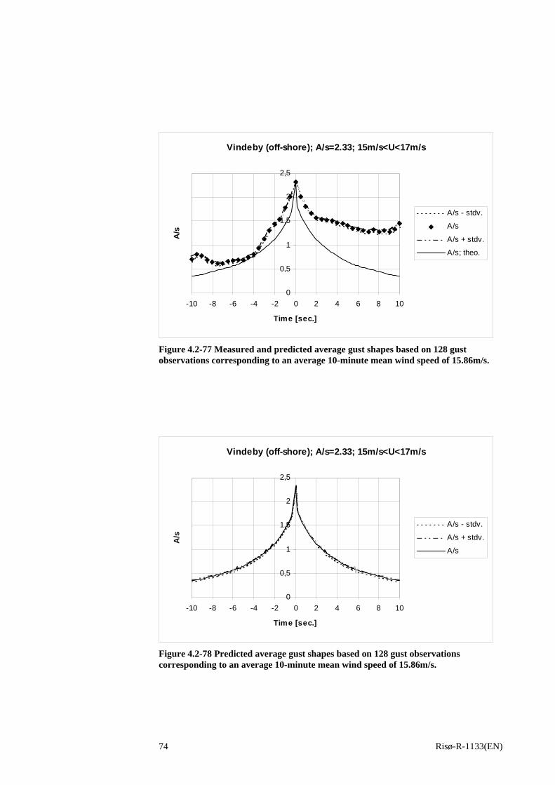
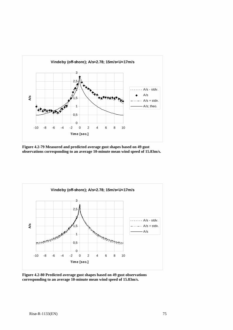
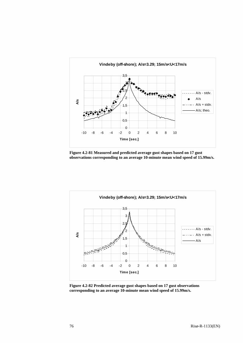
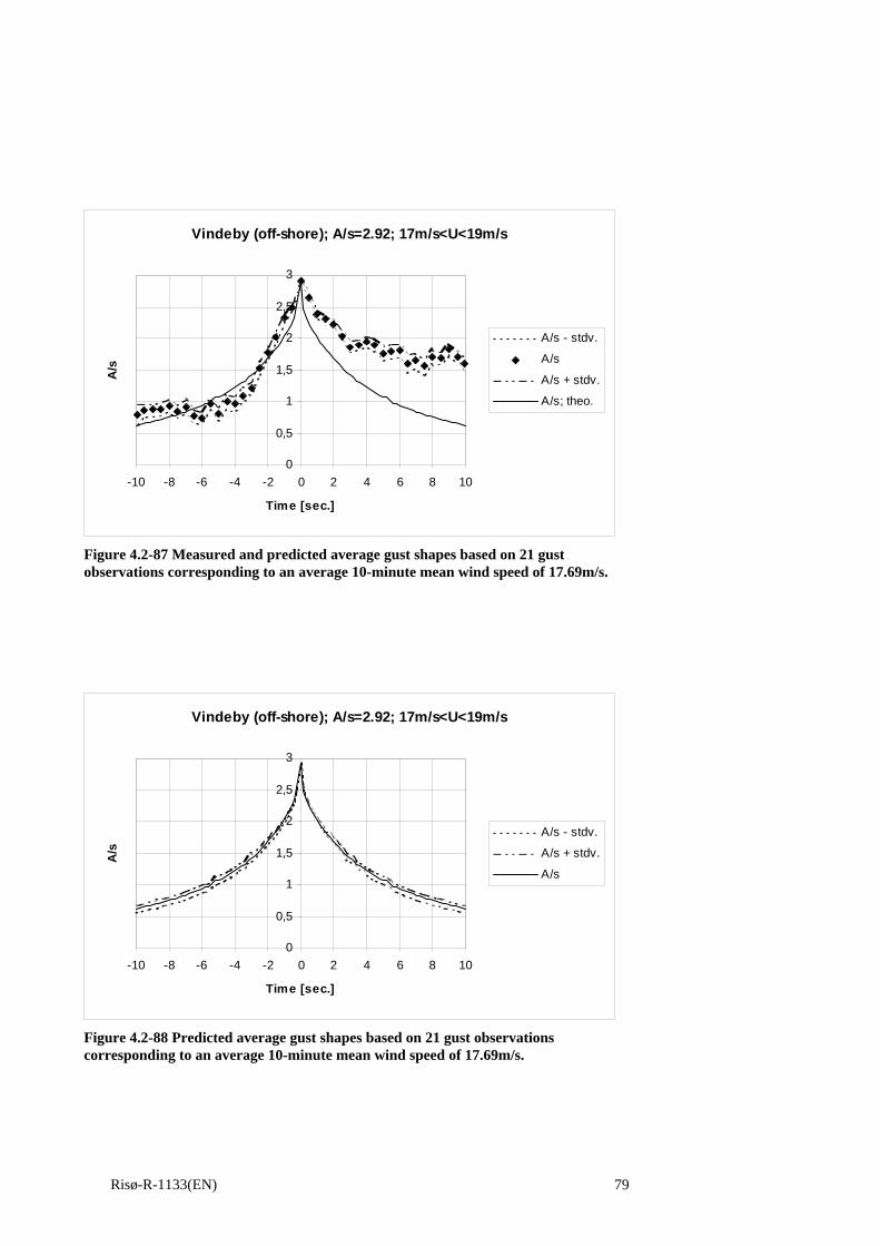
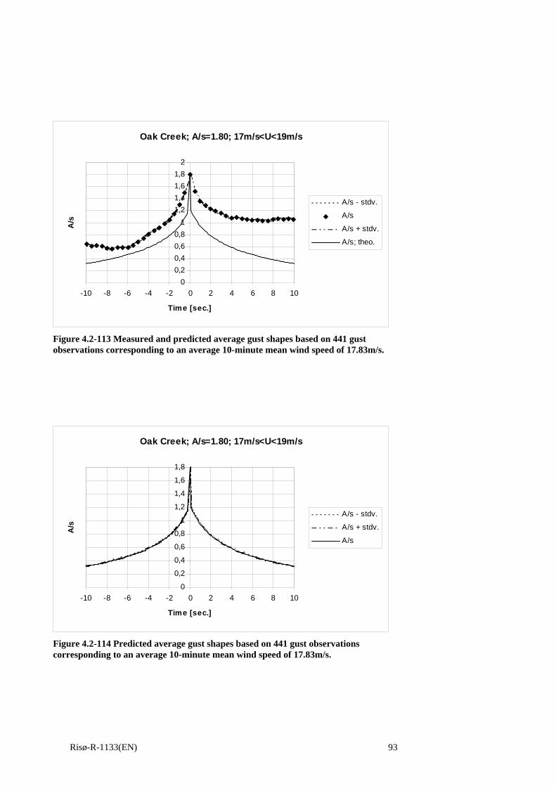
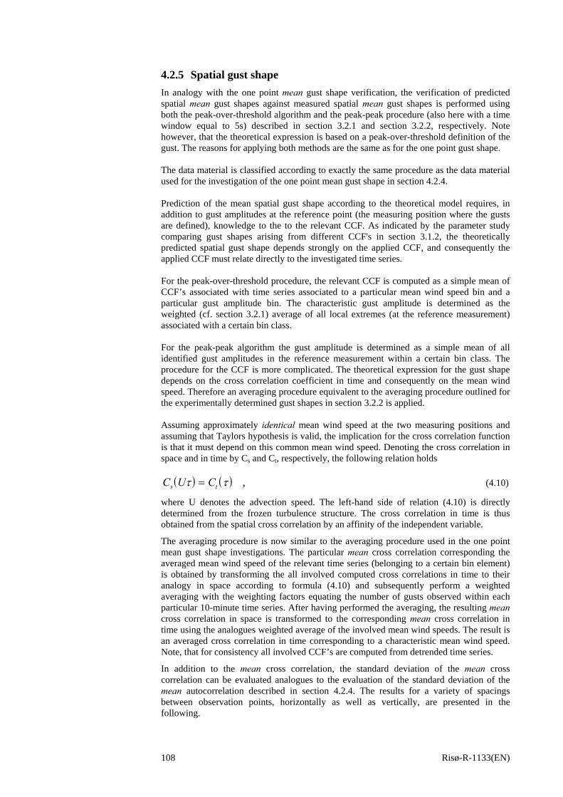
4.2 Wind field measurements In addition to simulated turbulence fields, the theoretical mean gust shape model is verified against (full-scale) meteorological measurements. The applied measurements are available from “Database on Wind Characteristics” (http://www.winddata.com/) - a huge WEB-database covering a vast amount of wind data measured at many different locations. Four different terrain conditions are considered - a shallow water offshore site, a flat coastal region, a flat and homogeneous inland terrain and a complex (mountainous) high wind site. The verification of predicted mean gust shapes against mean gust shapes, evaluated from the measured wind speed time series, is conducted using both the peak-over-threshold algorithm and the peak-peak procedure described in sections 3.2.1 and 3.2.2, respectively.
4.2.1 Data material It has been the intention to investigate a variety of different terrain types in order to make the analysis as “terrain independent” as possible. The particular choice of sites is in addition guided by considerations concerning amount of data, height of wind speed sensors above terrain, number of wind speed sensors and their mutual position, wind speed sample frequency, mean wind speed range and data quality. Four different terrain categories are investigated. These represent a shallow water offshore site, a flat coastal region, a flat and homogeneous inland terrain and a complex (mountainous) high wind site. The (shallow water) offshore terrain class is characterised by having open sea upstream conditions. The coastal terrain class encompasses flat coastal regions with water as well as land as upstream conditions. The upstream conditions for the flat and homogeneous terrain type is characterised by flat agricultural land and the
Risø-R-1133(EN) 25
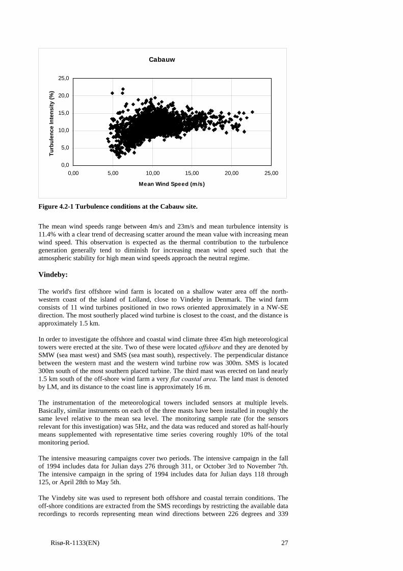
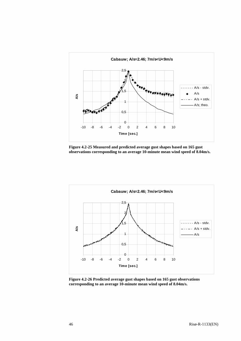
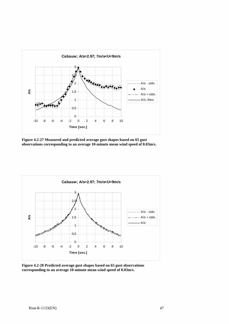
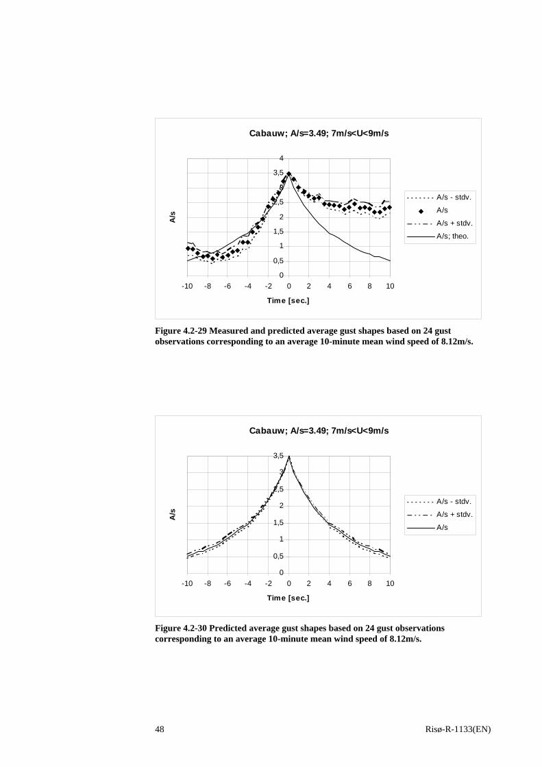
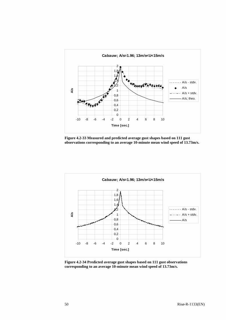
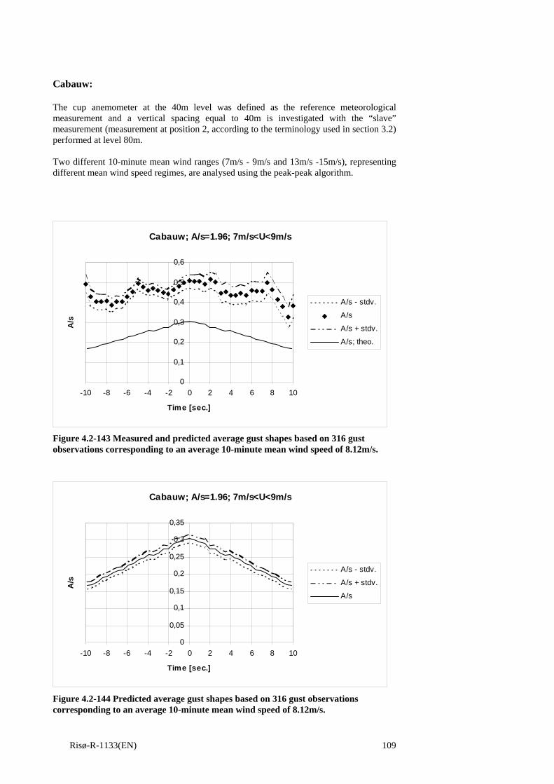
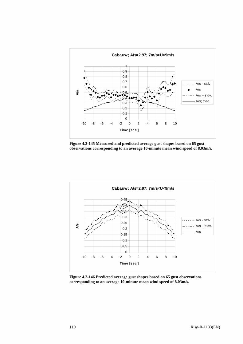
mountainous terrain is characterised by sharp terrain contours where flow separation is likely to take place. In section 4.1, the available amount of data is demonstrated to be important for a satisfactory averaging of the gust shape. Each of the selected sites therefore represents a substantial amount of data ranging between 2910 and 4470 10-minute time series. The measuring heights should preferably cover levels that are considered representative for the rotor area of present and future (within a horizon of 5 years) wind turbines. Thus heights varying between 20m and 80m are investigated. When analysing the spatial gust shape the reference sensor (the sensor defining the particular gust, cf. section 3.2) preferable represents the hub position, and thus hub heights ranging between 40m and 80m are investigated. The number of wind speed sensors as well as their mutual position become of importance when the spatial extension of the mean gust shape is investigated. The selected sites allow for vertical separations between measuring sensors ranging between 5m and 40m, and for one of the sites data from sensors with a horizontal separation are in addition available. The data quality and the sample frequency of the records are obviously of importance. The effect originating from the sample frequency was briefly investigated in section 4.1.5. In the present data material the sample frequency ranged between 2Hz and 8Hz. Finally, the mean wind speed is an important parameter as ultimate gust loading is likely to occur at high mean wind speeds. Therefore it is essential that high mean wind speeds (in the sense high for the particular site) site are represented. The four selected sites and the associated measuring system are described in details in the following. Cabauw: The Cabauw site is a Dutch site representing flat and homogeneous terrain conditions. A large meteorological tower is erected at the site. The meteorological mast is a tubular tower with a height of 213m and a diameter of 2m. Gay wires are attached at four levels. From 20m upwards horizontal trussed measurements booms are installed at intervals of 20m. At each level there are three booms, extending 10.4m from the centre line of the tower. These booms point to the directions 10, 130, 250 degrees relative to North. The SW and N booms are used for wind velocity and wind direction measurements. These booms carry at the end two lateral extensions with a length of 1.5m and a diameter of about 0.04m. The available amount of data consists of 2910 10-minute wind speed time series recorded from cup anemometers at levels 40m and 80m with a sample frequency of 2Hz. Figure (4.2.1), where the turbulence intensity is given as a function of the mean wind speed (evaluated at level 40m), gives an impression of the available wind speed recordings and the turbulence conditions at the site.
Risø-R-1133(EN) 26
Cabauw
0,0
5,0
10,0
15,0
20,0
25,0
0,00 5,00 10,00 15,00 20,00 25,00
Mean Wind Speed (m/s)
Turb
ulen
ce In
tens
ity (%
)
Figure 4.2-1 Turbulence conditions at the Cabauw site.
The mean wind speeds range between 4m/s and 23m/s and mean turbulence intensity is 11.4% with a clear trend of decreasing scatter around the mean value with increasing mean wind speed. This observation is expected as the thermal contribution to the turbulence generation generally tend to diminish for increasing mean wind speed such that the atmospheric stability for high mean wind speeds approach the neutral regime. Vindeby: The world's first offshore wind farm is located on a shallow water area off the north-western coast of the island of Lolland, close to Vindeby in Denmark. The wind farm consists of 11 wind turbines positioned in two rows oriented approximately in a NW-SE direction. The most southerly placed wind turbine is closest to the coast, and the distance is approximately 1.5 km. In order to investigate the offshore and coastal wind climate three 45m high meteorological towers were erected at the site. Two of these were located offshore and they are denoted by SMW (sea mast west) and SMS (sea mast south), respectively. The perpendicular distance between the western mast and the western wind turbine row was 300m. SMS is located 300m south of the most southern placed turbine. The third mast was erected on land nearly 1.5 km south of the off-shore wind farm a very flat coastal area. The land mast is denoted by LM, and its distance to the coast line is approximately 16 m. The instrumentation of the meteorological towers included sensors at multiple levels. Basically, similar instruments on each of the three masts have been installed in roughly the same level relative to the mean sea level. The monitoring sample rate (for the sensors relevant for this investigation) was 5Hz, and the data was reduced and stored as half-hourly means supplemented with representative time series covering roughly 10% of the total monitoring period. The intensive measuring campaigns cover two periods. The intensive campaign in the fall of 1994 includes data for Julian days 276 through 311, or October 3rd to November 7th. The intensive campaign in the spring of 1994 includes data for Julian days 118 through 125, or April 28th to May 5th. The Vindeby site was used to represent both offshore and coastal terrain conditions. The off-shore conditions are extracted from the SMS recordings by restricting the available data recordings to records representing mean wind directions between 226 degrees and 339
Risø-R-1133(EN) 27
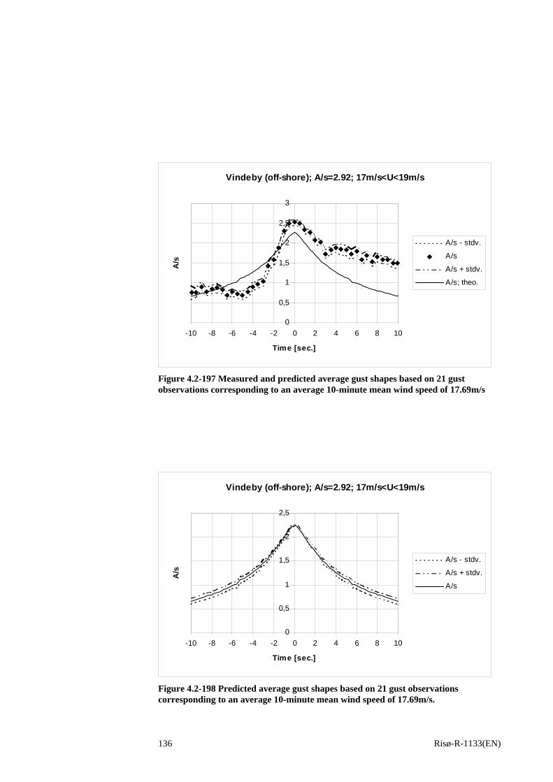
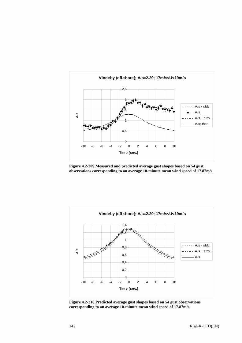
degrees (north equals zero degrees) such that in wake effects from the wind turbines are avoided. The coastal conditions are obtained from the LM recordings restricting the data material to recordings with mean wind direction ranging between 67 degrees and 251 degrees. The available amount of data describing the offshore situation consists of 4188 10-minute wind speed time series recorded from cup anemometers positioned at levels 48m, 43m and 38m. Figure (4.2.2), where the turbulence intensity is given as a function of the mean wind speed (evaluated at level 48m), gives an impression of the available wind speed recordings and the turbulence conditions for the offshore situation.
Vindeby (off-shore)
0,0
5,0
10,0
15,0
20,0
25,0
0,00 5,00 10,00 15,00 20,00 25,00
Mean Wind Speed (m/s)
Turb
ulen
ce In
tens
ity (%
)
Figure 4.2-2 Turbulence conditions at the Vindeby site (off-shore conditions).
A slight increasing turbulence intensity level with increasing mean wind speed is observed. This is due to increasing “terrain” roughness with increasing mean wind speed for offshore sites where the roughness elements is constituted by waves (Larsen, 1999). The mean turbulence intensity (for all mean wind speeds) is 6% with a standard deviation equal to 1.9%. Note that the scatter in the offshore turbulence intensities seems to be less sensitive to the size of the mean wind speed as the turbulence intensities reported from the Cabauw site. The effect of stability will be analysed in more details in section 4.2.2. The available amount of data describing the coastal situation consists of 3576 10-minute wind speed time series recorded from cup anemometers positioned at levels 46m, 38m and 20m. Figure (4.2.3), showing the turbulence intensity as a function of the mean wind speed (evaluated at level 46m), illustrates the available wind speed recordings and the turbulence conditions for the coastal situation. The mean wind speeds range in size from 5m/s to 21m/s, and the mean turbulence intensity (for all available mean wind speeds) is 10.3% with a standard deviation of 3.2%. The turbulence intensity level for the coastal site is of the same size as the turbulence intensity level for the Cabauw site. Note, however, the substantial increase in turbulence level (from an average value of 6% to an average value of 10.3%) compared to the offshore situation. As reported for the Cabauw site, the present coastal site display a tendency of decreasing scatter in the turbulence intensity with increasing mean wind speed. Also here, the explanation is related to a trend of change in atmospheric stability characteristics with the mean wind speed and this is analysed further in section 4.2.2.
Risø-R-1133(EN) 28
Vindeby (on-shore)
0,0
5,0
10,0
15,0
20,0
25,0
0,00 5,00 10,00 15,00 20,00 25,00
Mean Wind Speed (m/s)
Turb
ulen
ce In
tens
ity (%
)
Figure 4.2-3 Turbulence conditions at the Vindeby site (on-shore conditions).
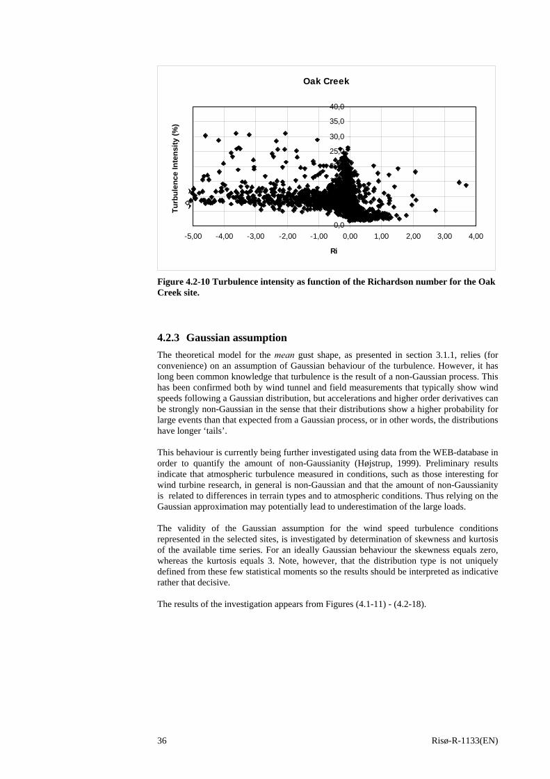
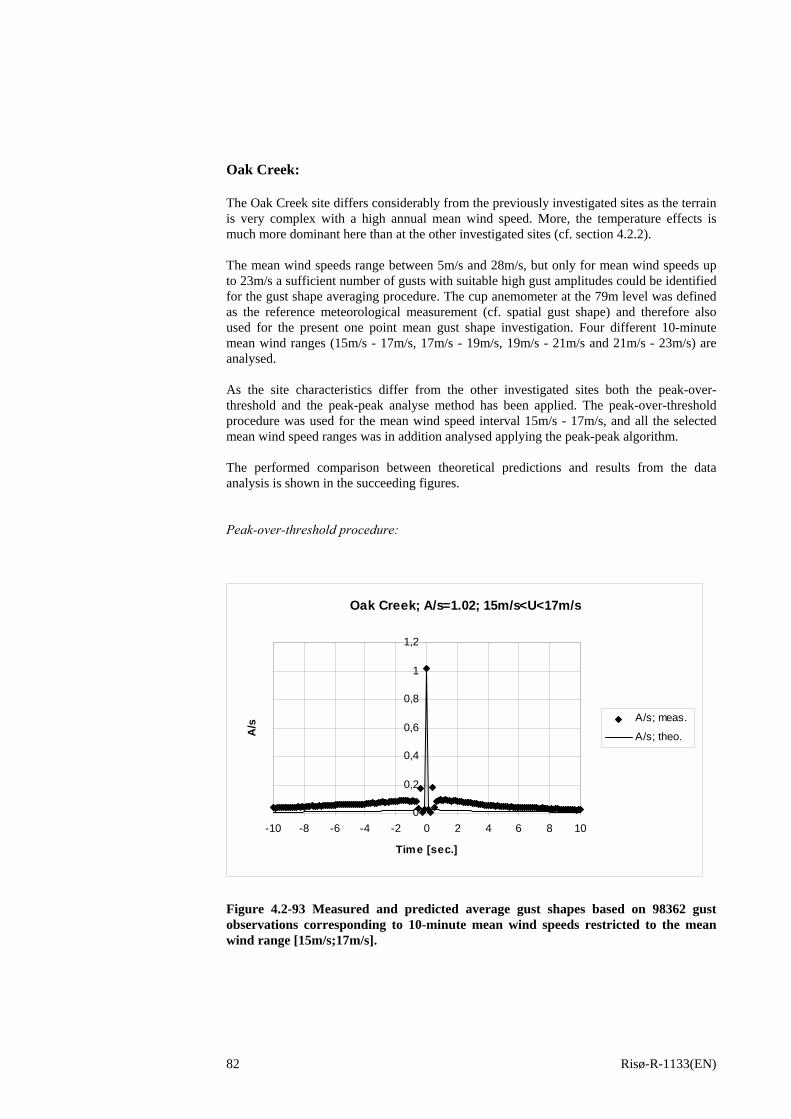
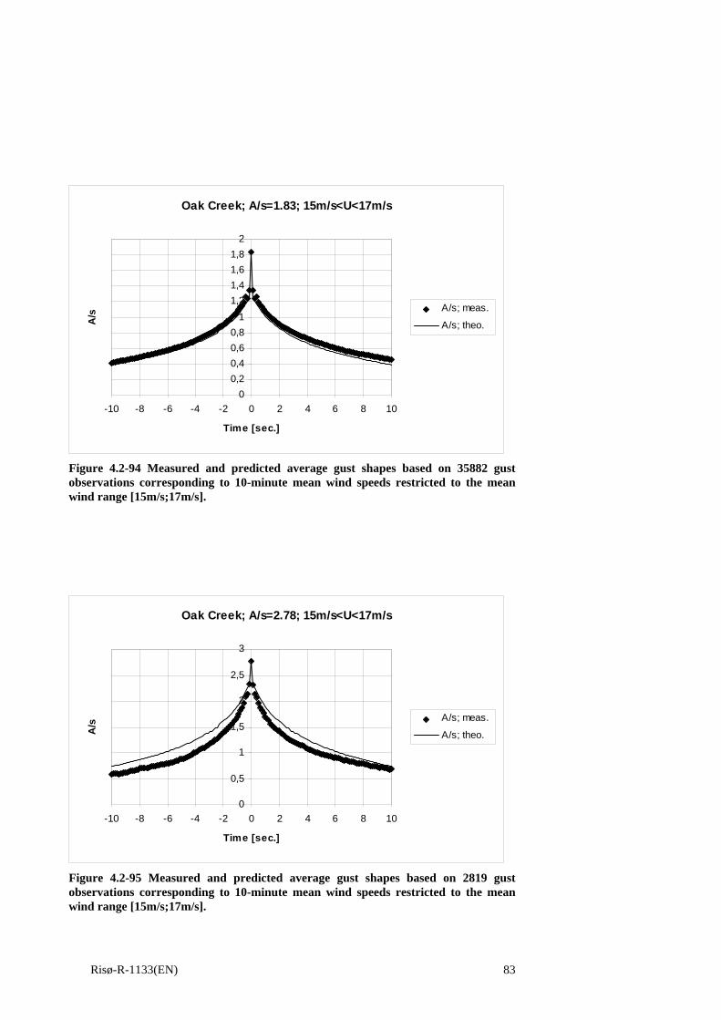
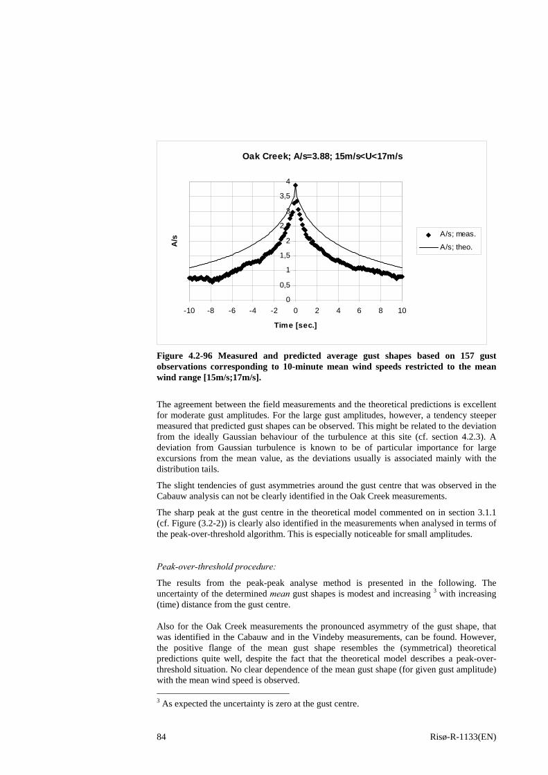
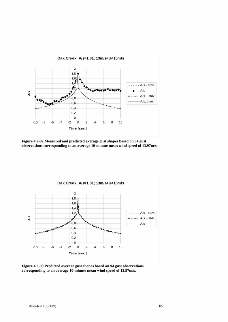
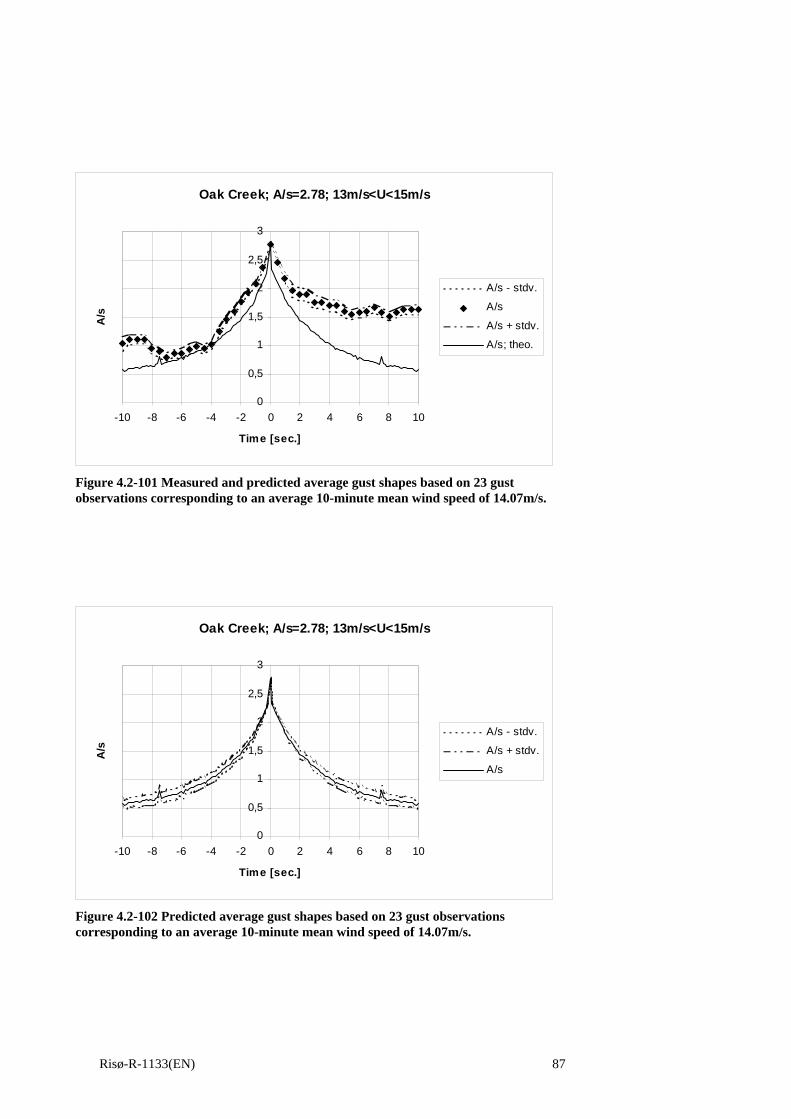
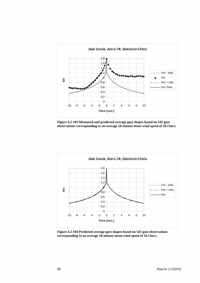
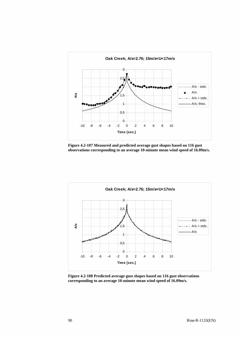
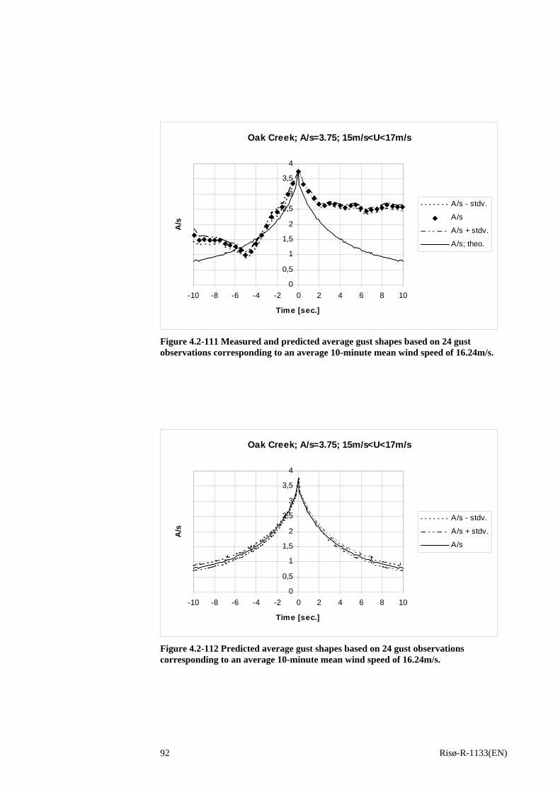
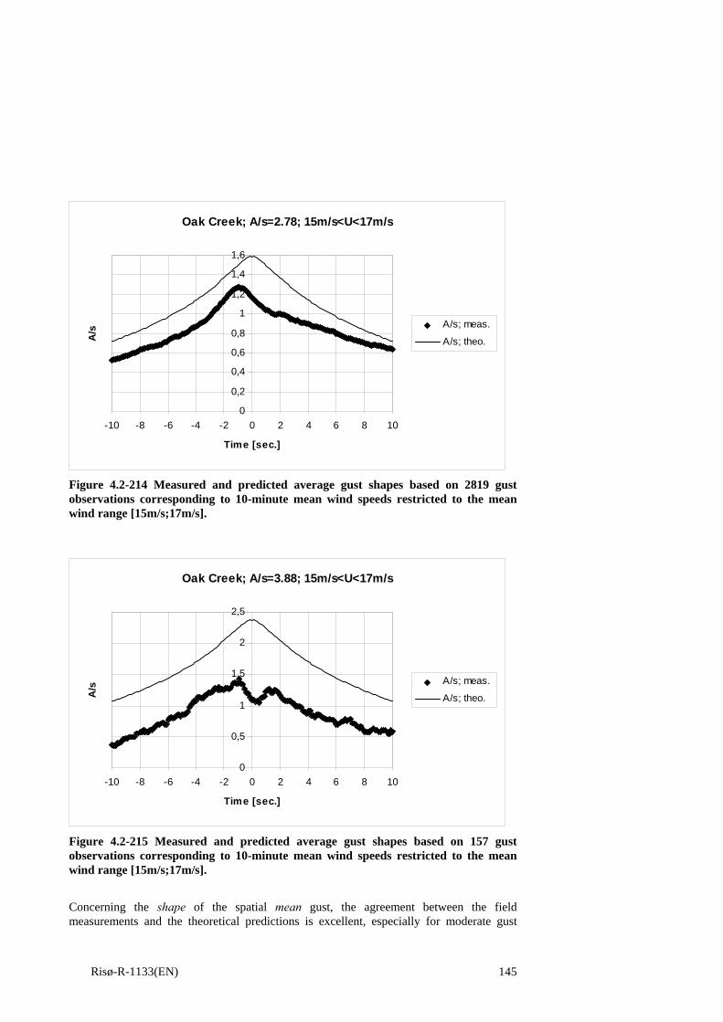
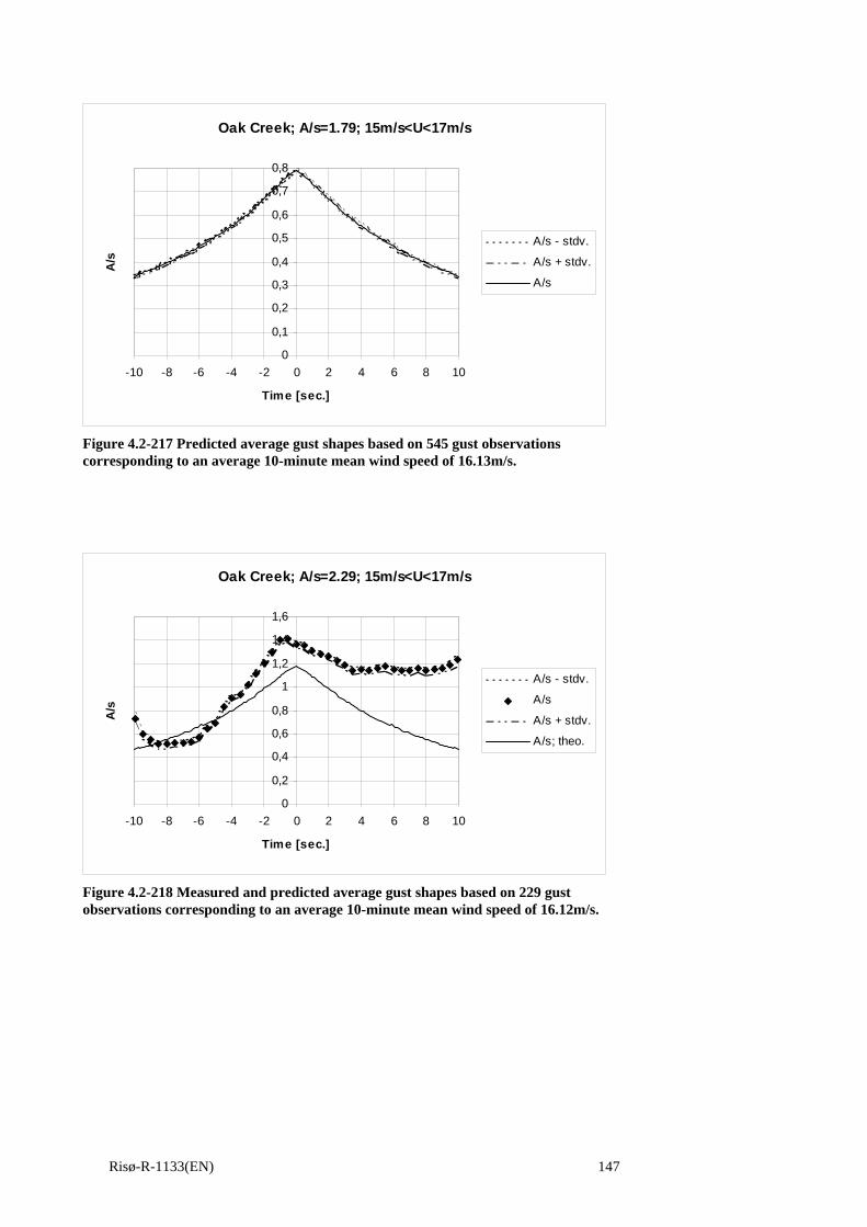
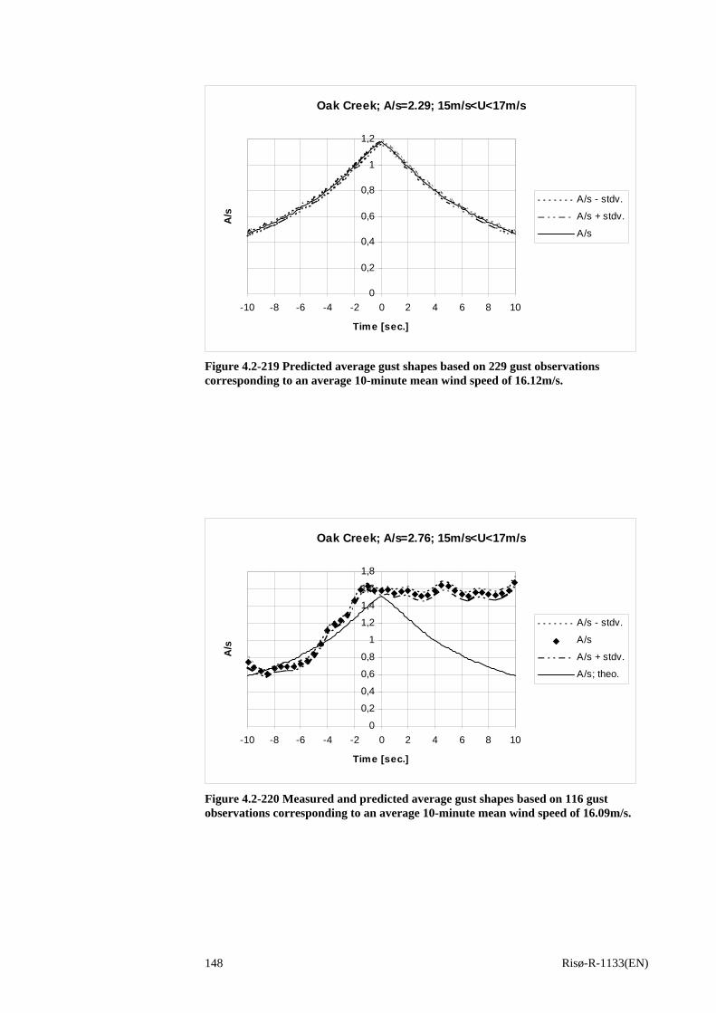
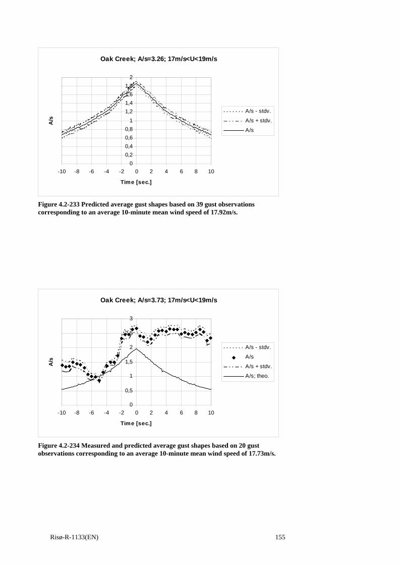
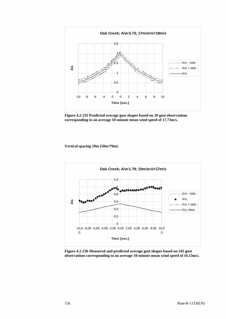
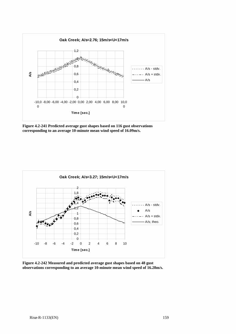
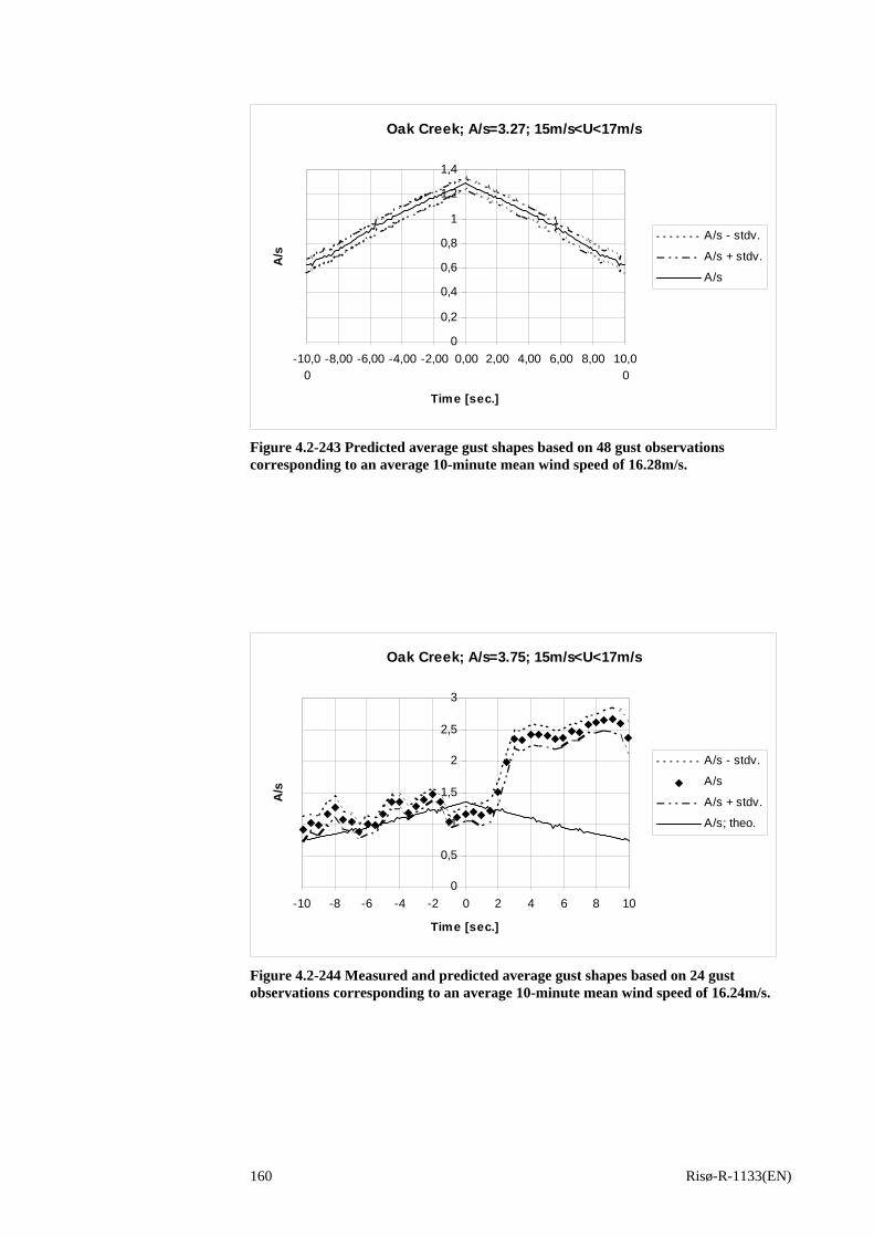
Oak Creek: Wind field measurements is currently being performed in a wind farm situated at a high wind (mountainous) site in Oak Creek, near Tehachapi in California. The measuring campaign is planned to continue during a one and a half year period, and at present data for a half year period are available. The purpose of the measurements is to gain knowledge of wind turbine loads caused by extreme wind load conditions. The wind field is measured from two 80m high meteorological towers erected at a ridge in the terrain. The distance between the two towers is 25.5m The meteorological towers are instrumented at several heights with both sonics and cup anemometers. Basically, similar instruments on each of the two masts are installed in roughly the same level relative to the terrain level. The monitoring system is running continuously, and the data are reduced and stored as 10-minutes statistics supplemented with intensive time series recordings covering periods where the mean wind speed exceeds a specified threshold (15 m/s) or the wind turbines operate in a transient load situation. The monitoring sample rate is 8Hz for the signals of relevance for the present investigation. In the present analysis, the cup anemometer wind speeds recorded at the levels 50m, 65m and 79m on mast 1 and level 79m on mast 2 are used. The choice enables us to investigate the vertical as well as the horizontal gust correlation. The available amount of data describing the mountainous terrain conditions consists of 4470 10-minute wind speed time series, and the character of the available data is illustrated in Figure (4.2-4) giving the turbulence intensity as function of the mean wind speed. The mean wind speeds range between 5/s and 28/s with the bulk of the data in the high wind regime above 15m/s. The mean turbulence intensity is 8.6% with a standard deviation equal to 4.6%. The most pronounced difference between the turbulence characteristics related to the mountainous terrain and the turbulence characteristics associated with the coastal- and the flat homogeneous sites is the increase the variability of the turbulence intensity, whereas the absolute levels are comparable. The trend of decreasing scatter around the mean value with increasing mean wind speed is very pronounced and shall be investigated further in section 4.2.2.
Risø-R-1133(EN) 29
Oak Creek
0,0
5,0
10,0
15,0
20,0
25,0
30,0
35,0
40,0
0,00 5,00 10,00 15,00 20,00 25,00 30,00
Mean Wind Speed (m/s)
Turb
ulen
ce In
tens
ity (%
)
Figure 4.2-4 Turbulence conditions at the Oak Creek site.
4.2.2 Atmospheric stability It is well known that the atmospheric stability may be of particular importance when investigating mean wind profiles as well as turbulence parameters, and therefore it is of potentially importance also for the present gust investigations. The stability conditions in the atmospheric boundary layer are traditionally classified as being unstable, neutral, or stable. Ideally, the neutral condition corresponds to a completely vertical stratification of the potential temperature, Θ, expressed by
Θ = +⎛
⎝⎜⎜
⎞
⎠⎟⎟T
gc
zp
,∆
(4.1)
where T denotes the absolute temperature, g is the acceleration of gravity, cp is the specific heat of atmospheric air at constant pressure, and ∆z is the height difference from the 1000mbar level. It is obvious that in this situation the thermal effects do not contribute (or more precisely is neutral in relation) to vertical exchange of momentum. In case of a potential temperature profile decreasing with the height, the temperature gradient contributes to the vertical exchange of energy and to the generation of turbulent eddies. This convective phenomenon characterises an unstable stratified boundary layer. Finally, stable atmospheric conditions are characterised by a potential temperature profile increasing with height. In this situation, the thermal effects tend to counteract the vertical exchange of momentum originating from mechanical generated turbulence. In a flow without shear, the potential temperature gradient is a suitable measure of the degree of stability/instability. However, when both thermal- and mechanical1 turbulence generating mechanisms contribute, the size of the potential temperature gradient is an inconvenient measure of the degree of stability as the vertical exchange of momentum is controlled not only by thermal effects but also of the mechanical turbulence production. Therefore, the stability conditions are often expressed in terms of the non-dimensional
1 Originating from the mean wind velocity shear.
Risø-R-1133(EN) 30
Richardson number, Ri, representing the relative importance of thermal generated buoyancy and mechanical generated shear in the turbulence production. A number of different versions of the Richardson number exist. However, due to its simplicity, the most widely used version is the gradient Richardson number defined according to
( )Ri
gT
z
U z=
∂ ∂
∂ ∂
Θ /
/,2 (4.2)
where z is the height above terrain level, and U and Θ denote the mean wind velocity and the mean potential temperature, respectively. The advantage of this particular Richardson number is that it contains only gradients of mean quantities that is easy to measure. According to the Monin-Obukhov similarity hypothesis2, various key atmospheric parameters, when non-dimensionalized with a scaling temperature or a scaling velocity, are expressed as universal functions of z/L. L denotes the Obukhov length which depends on the stability conditions in the boundary layer, but is independent of the level z. Using that, the variation of the Richardson number with the height can be expressed (Kaimal, 1994) as
Ri
zL
for unstableconditionszL
z Lz L
for stableconditionszL
=− ≤ ≤
+≤ ≤
⎧
⎨⎪
⎩⎪
( )/
/( )
2 0
1 50 1
(4.3)
In practice, the gradients in the expression for the Richardson number is evaluated by difference methods, and the question arises of which particular height the resulting Richardson number should be related to. Presuming near neutral conditions, where the mean velocity- and the mean potential temperature profiles exhibit a logarithmic dependence, an approximate pseudo height, zp, associated with the estimated Ri can be evaluated as
zz z
zz
p =−
⎛⎝⎜
⎞⎠⎟
2 121
ln, (4.4)
where z1 and z2 are the heights where (both) the velocity and temperature differences are evaluated from. Theoretically, the neutral situation is characterised by a zero Richardson number, whereas the stable and the unstable situation correspond to positive and negative values, respectively. The stability conditions tend to approach the neutral situation as the mean wind speed increases. However, in practice the neutral condition can obviously not be characterised by a single specific value of the Richardson number, but must rather be attached to a suitable Ri-interval around zero where neutral stratification is prevailing. The size of this interval is to some degree arbitrary, and in the following one possible approach is outlined. Considering the impact on turbulence originating from different stability conditions, the standard deviation of the vertical turbulence component, σw, is a reasonable descriptive measure. By means of Monin-Obukhov similarity, a parameterisation (Panofsky, 1983) can be expressed as
2 The hypothesis is based on empirical evidence gained from field experiments conducted over flat terrain.
Risø-R-1133(EN) 31
σ w
uz L for unstableconditions
z L for stableconditions∗
=−
+
⎧⎨⎩
(5 / )( / )(5 / )( (5 / ) ( / ))
/
/
4 1 34 1 2
1 3
1 3 (4.5)
Note, that as z/L is negative for unstable conditions and positive for stable conditions, the minimum value of the vertical variance is obtained for neutral atmospheric conditions. This might at first glance seems surprising as thermal effects at stable conditions tend to weaken the horizontal fluctuations. The explanation is the notably increased shear in the mean wind profile at stable conditions. Isolating the parameter z/L from relation (4.3) and subsequently introducing the result in the above expression (4.5) yields the following relation between the Richardson number and the standard deviation of the vertical turbulence component
[ ]σ w
uRi for unstableconditions
Ri Ri for stableconditions∗
=−
+ −
⎧⎨⎩
(5 / )( )(5 / )( (5 / ) ( / ))
/
/
4 1 34 1 2 1 5
1 3
1 3 (4.6)
From the above, the relative ratio between the standard deviation of the vertical turbulence component in general and the standard deviation of the vertical turbulence component at neutral conditions, σ0, is determined as
[ ]σσ
w Ri for unstableconditionsRi Ri for stableconditions0
1 3
1 3
1 31 2 1 5
=−
+ −
⎧⎨⎩
( )( (5 / ) ( / ))
/
/ (4.7)
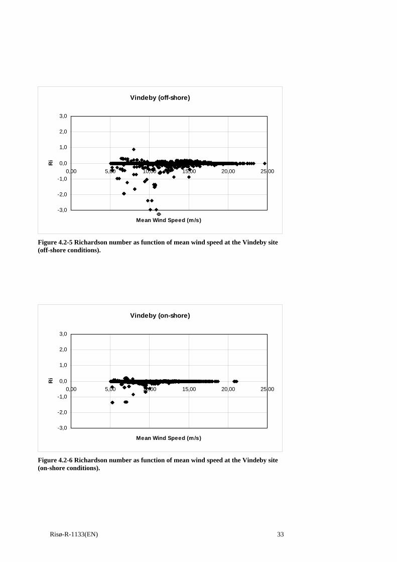
Choosing, rather arbitrarily, the "near neutral regime" to be limited by a maximum deviation (increase) in σw compared to σ0 of 25%, relation (4.7) yields the following limitations on the Richardson number related to near neutral conditions − ≤ ≤0 32 013. .Ri (4.8) The Richardson number, as formulated in relation (4.2), is computed for the measurements where temperature measurements, in addition to the wind speed recordings, are available - i.e. the off-shore site, the coastal site and the mountainous site. For each of these terrain conditions the Richardson number is plotted as function of the mean wind speed (at the levels where the turbulence intensity was computed in the investigations reported in section 4.2.1). The results are illustrated in the Figures (4.2-5-7). As indicated in section 4.2.1 it is expected that the atmospheric stability will tend towards neutral conditions for increasing mean wind speeds. This is confirmed by the investigation and, except for the Oak Creek site, the stability conditions can be characterised as neutral according to equation (4.8) for high mean wind speeds (which is anticipated to be of major importance in relation to gust loading). The Vindeby on-shore recordings display a very constant stability measure representing close to neutral stability conditions for almost the entire recorded mean wind speed range. The off-shore recordings shows a slightly increased scatter of the Richardson number around zero, however, for mean wind speeds exceeding 13m/s the stability measure is very stable representing neutral conditions according to relation (4.8). For the mountainous terrain the picture is different. The scatter in the stability measure is increased dramatically, and only for mean wind speeds exceeding 22m/s the stability conditions is stabilised.
Risø-R-1133(EN) 32
Vindeby (off-shore)
-3,0
-2,0
-1,0
0,0
1,0
2,0
3,0
0,00 5,00 10,00 15,00 20,00 25,00
Mean Wind Speed (m/s)
Ri
Figure 4.2-5 Richardson number as function of mean wind speed at the Vindeby site (off-shore conditions).
Vindeby (on-shore)
-3,0
-2,0
-1,0
0,0
1,0
2,0
3,0
0,00 5,00 10,00 15,00 20,00 25,00
Mean Wind Speed (m/s)
Ri
Figure 4.2-6 Richardson number as function of mean wind speed at the Vindeby site (on-shore conditions).
Risø-R-1133(EN) 33
Oak Creek
-40,0
-35,0
-30,0
-25,0
-20,0
-15,0
-10,0
-5,0
0,0
5,0
0,00 5,00 10,00 15,00 20,00 25,00 30,00
Mean Wind Speed (m/s)
Ri
Figure 4.2-7 Richardson number as function of mean wind speed at the Oak Creek site.
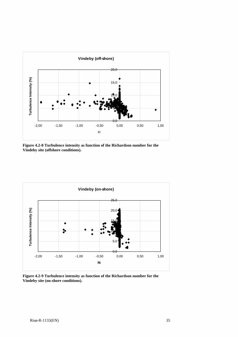
For each of these terrain conditions the Richardson number is plotted as function of the mean wind speed (at the levels where the turbulence intensity was computed in the investigations reported in section 4.2.1). The results are illustrated in the Figures (4.2-5), (4.2-6) and (4.2-7). As indicated in section 4.2.1 it is expected that the atmospheric stability will tend towards neutral conditions for increasing mean wind speeds. This is confirmed by the investigation and, except for the Oak Creek site, the stability conditions can be characterised as neutral according to equation (4.8) for high mean wind speeds (which is anticipated to be of major importance in relation to gust loading). The gust mean shape is mainly investigated for relative large mean wind speeds, and based on the above stability investigations it was decided not to split the investigation into different stability regimes. However, for the Oak Creek site, the exercise could be meaning full in the low and medium mean wind speed range - off course at the expense of reducing the available number of data recordings for the gust shape averaging procedure. The decision is further supported by inspection of the Figures (4.2-8), (4.2-9) and (4.2-10), where the turbulence intensity is plotted as function of the Richardson number. Except for the stable regime, there is no indication of a dramatic change in the mean turbulence intensity level with the Richardson number.
Risø-R-1133(EN) 34
Vindeby (off-shore)
0,0
5,0
10,0
15,0
20,0
-2,00 -1,50 -1,00 -0,50 0,00 0,50 1,00
ri
Turb
ulen
ce In
tens
ity (%
)
Figure 4.2-8 Turbulence intensity as function of the Richardson number for the Vindeby site (offshore conditions).
Vindeby (on-shore)
0,0
5,0
10,0
15,0
20,0
25,0
-2,00 -1,50 -1,00 -0,50 0,00 0,50 1,00
Ri
Turb
ulen
ce In
tens
ity (%
)
Figure 4.2-9 Turbulence intensity as function of the Richardson number for the Vindeby site (on-shore conditions).
Figure 4.2-10 Turbulence intensity as function of the Richardson number for the Oak Creek site.
4.2.3 Gaussian assumption The theoretical model for the mean gust shape, as presented in section 3.1.1, relies (for convenience) on an assumption of Gaussian behaviour of the turbulence. However, it has long been common knowledge that turbulence is the result of a non-Gaussian process. This has been confirmed both by wind tunnel and field measurements that typically show wind speeds following a Gaussian distribution, but accelerations and higher order derivatives can be strongly non-Gaussian in the sense that their distributions show a higher probability for large events than that expected from a Gaussian process, or in other words, the distributions have longer ‘tails’. This behaviour is currently being further investigated using data from the WEB-database in order to quantify the amount of non-Gaussianity (Højstrup, 1999). Preliminary results indicate that atmospheric turbulence measured in conditions, such as those interesting for wind turbine research, in general is non-Gaussian and that the amount of non-Gaussianity is related to differences in terrain types and to atmospheric conditions. Thus relying on the Gaussian approximation may potentially lead to underestimation of the large loads. The validity of the Gaussian assumption for the wind speed turbulence conditions represented in the selected sites, is investigated by determination of skewness and kurtosis of the available time series. For an ideally Gaussian behaviour the skewness equals zero, whereas the kurtosis equals 3. Note, however, that the distribution type is not uniquely defined from these few statistical moments so the results should be interpreted as indicative rather that decisive. The results of the investigation appears from Figures (4.1-11) - (4.2-18).
Risø-R-1133(EN) 36
Cabauw
-3,0
-2,0
-1,0
0,0
1,0
2,0
3,0
0,00 5,00 10,00 15,00 20,00 25,00
Mean Wind Speed (m/s)
Skew
ness
Figure 4.2-11 Skewness plotted as function of mean wind speed for 2233 10-minutes time series originating from the Cabauw site.
Cabauw
1,0
2,0
3,0
4,0
5,0
6,0
7,0
0,00 5,00 10,00 15,00 20,00 25,00
Mean Wind Speed (m/s)
Kur
tosi
s
Figure 4.2-12 Kurtosis plotted as function of mean wind speed for 2233 10-minutes time series originating from the Cabauw site.
For a Gaussian all even order moments are zero, and the fourth (kurtosis) moment equal to 3. Mean value of skewness and kurtosis for all analysed time series is 0.023 and 2.825, respectively, it is quite obvious that in this case velocities are close to being Gaussian when evaluated in terms of the third and forth order moment.
Risø-R-1133(EN) 37
Vindeby (on-shore)
-3,0
-2,0
-1,0
0,0
1,0
2,0
3,0
0,00 5,00 10,00 15,00 20,00 25,00
Mean Wind Speed (m/s)
Skew
ness
Figure 4.2-13 Skewness plotted as function of mean wind speed for 3576 10-minutes time series originating from the Vindeby site (on-shore sector from the land mast).
Vindeby (on-shore)
1,0
3,0
5,0
7,0
9,0
11,0
13,0
15,0
0,00 5,00 10,00 15,00 20,00 25,00
Mean Wind Speed (m/s)
Kur
tosi
s
Figure 4.2-14 Kurtosis plotted as function of mean wind speed for 3576 10-minutes time series originating from the Vindeby site (on-shore sector from the land mast).
Mean value of skewness and kurtosis for all analysed time series is -0.089 and 2.838, with standard deviations 0.312 and 0.470, respectively, and also for these data the velocities are close to being Gaussian when evaluated in terms of the third and forth order moment.
Risø-R-1133(EN) 38
Vindeby (off-shore)
-3,0
-2,0
-1,0
0,0
1,0
2,0
3,0
0,00 5,00 10,00 15,00 20,00 25,00
Mean Wind Speed (m/s)
Skew
ness
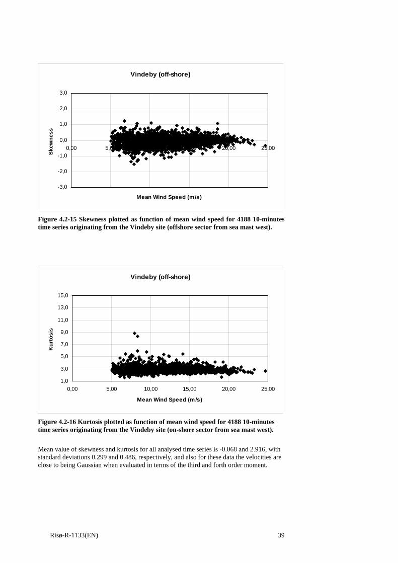
Figure 4.2-15 Skewness plotted as function of mean wind speed for 4188 10-minutes time series originating from the Vindeby site (offshore sector from sea mast west).
Vindeby (off-shore)
1,0
3,0
5,0
7,0
9,0
11,0
13,0
15,0
0,00 5,00 10,00 15,00 20,00 25,00
Mean Wind Speed (m/s)
Kur
tosi
s
Figure 4.2-16 Kurtosis plotted as function of mean wind speed for 4188 10-minutes time series originating from the Vindeby site (on-shore sector from sea mast west).
Mean value of skewness and kurtosis for all analysed time series is -0.068 and 2.916, with standard deviations 0.299 and 0.486, respectively, and also for these data the velocities are close to being Gaussian when evaluated in terms of the third and forth order moment.
Risø-R-1133(EN) 39
Oak Creek
-3,0
-2,0
-1,0
0,0
1,0
2,0
3,0
0,00 5,00 10,00 15,00 20,00 25,00 30,00
Mean Wind Speed (m/s)
Skew
ness
Figure 4.2-17 Skewness plotted as function of mean wind speed for 4470 10-minutes time series originating from the Oak Creek site.
Oak Creek
1,0
3,0
5,0
7,0
9,0
11,0
13,0
15,0
0,00 5,00 10,00 15,00 20,00 25,00 30,00
Mean Wind Speed (m/s)
Kur
tosi
s
Figure 4.2-18 Kurtosis plotted as function of mean wind speed for 4470 10-minutes time series originating from the Oak Creek site.
Mean value of skewness and kurtosis for all analysed time series is -0.479 and 3.543, with standard deviations 0.479 and 1.625, respectively. It is concluded that for the Oak Creek data the velocities differ somewhat from being Gaussian when evaluated in terms of the third and forth order moment, although the scatter is these values are considerable especially for the high wind situations with 10-minute mean wind speeds exceeding 15m/s.
Risø-R-1133(EN) 40
4.2.4 One point mean gust shape The verification of predicted mean gust shapes against observed mean gust shapes, as evaluated from the measured wind speed time series from the investigated sites, is conducted using both the peak-over-threshold algorithm and the peak-peak procedure (with a time window equal to 5s) described in section 3.2.1 and section 3.2.2, respectively. It should, however, be noted that the theoretical model is based on a peak-over-threshold definition of the gust. The peak-over-threshold definition of gust seems logical for structures where only the peak value is of importance. For a wind turbine, the dynamic character of the loading is often vital - this is especially true for pitch regulated turbines where the time constants in the control system in addition is an important factor. Both analysis methods requires that the available data material is classified according to a bin matrix in two dimensions - the 10-minute mean wind speed and the gust amplitude. The mean wind speed range is divided into bins each of an extend equal to 2m/s. The gusts amplitudes are (generally) classified in 5 groups depending on the ratio between the gust amplitude and the (de-trended) standard deviation associated with the particular time series. The ratio intervals defining the classes were 1.75-2.25, 2.25-2.75, 2.75-3.25, 3.25-3.75 and above 3.75. Prediction of the mean gust shape according to the theoretical model requires, in addition to gust amplitudes, knowledge to the to a relevant ACF. As indicated by the parameter study comparing gust shapes arising from different ACF’s in section 3.1.1, the theoretically predicted gust shape depends strongly on the applied ACF. Therefore the applied ACF must relate directly to the investigated time series. For the peak-over-threshold procedure, the relevant ACF is computed as a simple mean of ACF’s associated with the time series representing a particular bin-element. The gust amplitude is determined as the weighted (cf. section 3.2.1) average of all local extremes associated with a certain bin class. For the peak-peak algorithm a gust amplitude is determined as a simple mean of identified gust amplitudes within a certain bin class. The procedure for the ACF is a little more involved. The theoretical expression for the gust shape depends on the autocorrelation coefficient in time and consequently on the mean wind speed. Therefore an averaging procedure equivalent to the averaging procedure outlined for the experimentally determined gust shapes in section 3.2.2 is applied. Retaining to Taylors hypothesis, the implication for the autocorrelation function is that it must depend on the mean wind speed. Denoting the autocorrelation in space and in time by Rs and Rt, respectively, the following relation holds
( ) ( )R U Rs tτ τ= , (4.9)
where U denotes the advection speed (the mean wind speed). The left hand side of relation (4.9) is directly determined from the frozen turbulence structure. The autocorrelation in time is thus obtained from the spatial autocorrelation by an affinity of the independent variable.
The particular mean autocorrelation corresponding the averaged mean wind speed of the relevant time series (belonging to a certain bin element) is obtained by transforming the all involved computed autocorrelations in time to their analogy in space according to formula (4.9) and subsequently perform a weighted averaging with the weighting factors equating the number of gusts observed within each particular 10-minute time series. After having performed the averaging, the resulting mean autocorrelation in space is transformed to the corresponding mean autocorrelation in time using the analogues weighted average of the involved mean wind speeds. The result is an averaged autocorrelation in time corresponding to a distinct (characteristic) mean wind speed, as was also the outcome of the procedure for determining the experimental mean gust shape in section 3.2.2. Note, that for consistency all involved ACF’s are computed from de-trended time series.
Risø-R-1133(EN) 41
In addition to the mean autocorrelation, the standard deviation of the mean autocorrelation is evaluated by determining the standard deviation of the autocorrelation in space within a suitable selected spatial interval. Assuming the deviations in the autocorrelation, at a given spatial co-ordinate, to be Gaussian distributed, the standard deviation on the mean autocorrelation in space, at the particular spatial co-ordinate, is estimated by dividing the calculated standard deviation with the square root of the number of averaged gusts. The estimated standard deviation of the mean autocorrelation, at a given spatial position, is finally transformed to standard deviation of the mean autocorrelation in the time by dividing the spatial co-ordinate with the calculated average (characteristic) mean wind speed. The results for the 4 sites is presented in the following. Cabauw: The mean wind speeds range between 4m/s and 23m/s, but only for mean wind speeds up to 15m/s a sufficient number of gusts with suitable high gust amplitudes could be identified for the gust shape averaging procedure. The cup anemometer at the 40m level was defined as the reference meteorological measurement (cf. spatial gust shape) and consequently used for the present one point mean gust shape investigation. Three different 10-minute mean wind ranges (7m/s - 9m/s, 9m/s - 11m/s and 13m/s -15m/s), representing different mean wind speed regimes (medium to high mean wind speeds), are analysed. The peak-over-threshold procedure was used for the mean wind speed interval 9m/s - 11m/s, whereas the two remaining mean wind speed intervals was analysed applying the peak-peak algorithm. A priori, the Taylor hypothesis, applied in the averaging procedure for the peak-peak procedure, is expected to be best satisfied for high mean wind speeds. The performed comparison between theoretical predictions and results from the data analysis is shown in the succeeding figures, where A denotes the gust amplitude and s is the (de-trended) wind speed standard deviation. Peak-over-threshold procedure:
Cabauw; A/s=1.01; 9m/s<U<11m/s
-0,4
-0,2
0
0,2
0,4
0,6
0,8
1
1,2
-10 -8 -6 -4 -2 0 2 4 6 8 10
Time [sec.]
A/s A/s; meas.
A/s; theo.
Figure 4.2-19 Measured and predicted average gust shapes based on 17701 gust observations corresponding to 10-minute mean wind speeds restricted to the range [9m/s;11m/s].
Risø-R-1133(EN) 42
Cabauw; A/s=1.89; 9m/s<U<11m/s
00,20,40,60,8
11,21,41,61,8
2
-10 -8 -6 -4 -2 0 2 4 6 8 10
Time [sec.]
A/s A/s; meas.
A/s; theo.
Figure 4.2-20 Measured and predicted average gust shapes based on 9331 gust observations corresponding to 10-minute mean wind speeds restricted to the range [9m/s;11m/s].
Cabauw; A/s=2.8; 9m/s<U<11m/s
0
0,5
1
1,5
2
2,5
3
-10 -8 -6 -4 -2 0 2 4 6 8 10
Time [sec.]
A/s A/s; meas.
A/s; theo.
Figure 4.2-21 Measured and predicted average gust shapes based on 1335 gust observations corresponding to 10-minute mean wind speeds restricted to the range [9m/s;11m/s].
Risø-R-1133(EN) 43
Cabauw; A/s=3.9; 9m/s<U<11m/s
0
0,5
1
1,5
2
2,5
3
3,5
4
-10 -8 -6 -4 -2 0 2 4 6 8 10
Time [sec.]
A/s A/s; meas.
A/s; theo.
Figure 4.2-22 Measured and predicted average gust shapes based on 80 gust observations corresponding to 10-minute mean wind speeds restricted to the range [9m/s;11m/s].
The agreement between the field measurements and the theoretical predictions is good, especially for moderately large gust amplitudes where a large amount of local extremes is contributing to the gust shape averaging procedure. Slight tendencies of gust asymmetries around the gust centre can be observed for relative large gust amplitudes, but whether this phenomenon is caused by non-Gaussian behaviour of large turbulence excursions (cf. section 4.2.3), or rather a result of the decreasing number of local extremes in the gust shape averaging procedure is not clear.
Peak-over-threshold procedure:
The results from the peak-peak analyse method is presented in the following. For each bin class two plots are given.
In the first (upper), the measured mean gust shape is compared with the theoretically predicted mean gust shape as based on the computed mean ACF. In addition the measured mean gust shape plus and minus one standard deviation has been shown.
In the second (the lower) the computed mean ACF is shown together with the mean ACF plus and minus one standard deviation.
It is characteristic that the uncertainty of the determined mean gust shapes is modest. As expected the uncertainty is zero at the gust amplitude and increasing with increasing distance from the gust centre.
Risø-R-1133(EN) 44
Cabauw; A/s=1.96; 7m/s<U<9m/s
00,20,40,60,8
11,21,41,61,8
2
-10 -8 -6 -4 -2 0 2 4 6 8 10
Time [sec.]
A/s
A/s - stdv.
A/s
A/s + stdv.
A/s; theo.
Figure 4.2-23 Measured and predicted average gust shapes based on 316 gust observations corresponding to an average 10-minute mean wind speed of 8.12m/s.
Cabauw; A/s=1.96; 7m/s<U<9m/s
00,20,40,60,8
11,21,41,61,8
2
-10 -8 -6 -4 -2 0 2 4 6 8 10
Time [sec.]
A/s
A/s - stdv.
A/s + stdv.
A/s
Figure 4.2-24 Predicted average gust shapes based on 316 gust observations corresponding to an average 10-minute mean wind speed of 8.12m/s.
Risø-R-1133(EN) 45
Cabauw; A/s=2.46; 7m/s<U<9m/s
0
0,5
1
1,5
2
2,5
-10 -8 -6 -4 -2 0 2 4 6 8 10
Time [sec.]
A/s
A/s - stdv.
A/s
A/s + stdv.
A/s; theo.
Figure 4.2-25 Measured and predicted average gust shapes based on 165 gust observations corresponding to an average 10-minute mean wind speed of 8.04m/s.
Cabauw; A/s=2.46; 7m/s<U<9m/s
0
0,5
1
1,5
2
2,5
-10 -8 -6 -4 -2 0 2 4 6 8 10
Time [sec.]
A/s
A/s - stdv.
A/s + stdv.
A/s
Figure 4.2-26 Predicted average gust shapes based on 165 gust observations corresponding to an average 10-minute mean wind speed of 8.04m/s.
Risø-R-1133(EN) 46
Cabauw; A/s=2.97; 7m/s<U<9m/s
0
0,5
1
1,5
2
2,5
3
-10 -8 -6 -4 -2 0 2 4 6 8 10
Time [sec.]
A/s
A/s - stdv.
A/s
A/s + stdv.
A/s; theo.
Figure 4.2-27 Measured and predicted average gust shapes based on 65 gust observations corresponding to an average 10-minute mean wind speed of 8.03m/s.
Cabauw; A/s=2.97; 7m/s<U<9m/s
0
0,5
1
1,5
2
2,5
3
-10 -8 -6 -4 -2 0 2 4 6 8 10
Time [sec.]
A/s
A/s - stdv.
A/s + stdv.
A/s
Figure 4.2-28 Predicted average gust shapes based on 65 gust observations corresponding to an average 10-minute mean wind speed of 8.03m/s.
Risø-R-1133(EN) 47
Cabauw; A/s=3.49; 7m/s<U<9m/s
0
0,5
1
1,5
2
2,5
3
3,5
4
-10 -8 -6 -4 -2 0 2 4 6 8 10
Time [sec.]
A/s
A/s - stdv.
A/s
A/s + stdv.
A/s; theo.
Figure 4.2-29 Measured and predicted average gust shapes based on 24 gust observations corresponding to an average 10-minute mean wind speed of 8.12m/s.
Cabauw; A/s=3.49; 7m/s<U<9m/s
0
0,5
1
1,5
2
2,5
3
3,5
-10 -8 -6 -4 -2 0 2 4 6 8 10
Time [sec.]
A/s
A/s - stdv.
A/s + stdv.
A/s
Figure 4.2-30 Predicted average gust shapes based on 24 gust observations corresponding to an average 10-minute mean wind speed of 8.12m/s.
Risø-R-1133(EN) 48
Cabauw; A/s=3.98; 7m/s<U<9m/s
0
0,5
1
1,5
2
2,5
3
3,5
4
4,5
-10 -8 -6 -4 -2 0 2 4 6 8 10
Time [sec.]
A/s
A/s - stdv.
A/s
A/s + stdv.
A/s; theo.
Figure 4.2-31 Measured and predicted average gust shapes based on 12 gust observations corresponding to an average 10-minute mean wind speed of 7.86m/s.
Cabauw; A/s=3.98; 7m/s<U<9m/s
0
0,5
1
1,5
2
2,5
3
3,5
4
-10 -8 -6 -4 -2 0 2 4 6 8 10
Time [sec.]
A/s
A/s - stdv.
A/s + stdv.
A/s
Figure 4.2-32 Predicted average gust shapes based on 12 gust observations corresponding to an average 10-minute mean wind speed of 7.86m/s.
Risø-R-1133(EN) 49
Cabauw; A/s=1.96; 13m/s<U<15m/s
00,20,40,60,8
11,21,41,61,8
2
-10 -8 -6 -4 -2 0 2 4 6 8 10
Time [sec.]
A/s
A/s - stdv.
A/s
A/s + stdv.
A/s; theo.
Figure 4.2-33 Measured and predicted average gust shapes based on 111 gust observations corresponding to an average 10-minute mean wind speed of 13.73m/s.
Cabauw; A/s=1.96; 13m/s<U<15m/s
00,20,40,60,8
11,21,41,61,8
2
-10 -8 -6 -4 -2 0 2 4 6 8 10
Time [sec.]
A/s
A/s - stdv.
A/s + stdv.
A/s
Figure 4.2-34 Predicted average gust shapes based on 111 gust observations corresponding to an average 10-minute mean wind speed of 13.73m/s.
Risø-R-1133(EN) 50
Cabauw; A/s=2.47; 13m/s<U<15m/s
0
0,5
1
1,5
2
2,5
-10 -8 -6 -4 -2 0 2 4 6 8 10
Time [sec.]
A/s
A/s - stdv.
A/s
A/s + stdv.
A/s; theo.
Figure 4.2-35 Measured and predicted average gust shapes based on 64 gust observations corresponding to an average 10-minute mean wind speed of 13.81m/s.
Cabauw; A/s=2.47; 13m/s<U<15m/s
0
0,5
1
1,5
2
2,5
-10 -8 -6 -4 -2 0 2 4 6 8 10
Time [sec.]
A/s
A/s - stdv.
A/s + stdv.
A/s
Figure 4.2-36 Predicted average gust shapes based on 64 gust observations corresponding to an average 10-minute mean wind speed of 13.81m/s.
Risø-R-1133(EN) 51
Cabauw; A/s=2.93; 13m/s<U<15m/s
0
0,5
1
1,5
2
2,5
3
-10 -8 -6 -4 -2 0 2 4 6 8 10
Time [sec.]
A/s
A/s - stdv.
A/s
A/s + stdv.
A/s; theo.
Figure 4.2-37 Measured and predicted average gust shapes based on 19 gust observations corresponding to an average 10-minute mean wind speed of 13.89m/s.
Cabauw; A/s=2.93; 13m/s<U<15m/s
0
0,5
1
1,5
2
2,5
3
-10 -8 -6 -4 -2 0 2 4 6 8 10
Time [sec.]
A/s
A/s - stdv.
A/s + stdv.
A/s
Figure 4.2-38 Predicted average gust shapes based on 19 gust observations corresponding to an average 10-minute mean wind speed of 13.89m/s.
Risø-R-1133(EN) 52
It is characteristic that the measured results, when analysed according the peak-peak procedure, display a pronounced asymmetry around the gust amplitude of the mean gust shape. However, the positive flange of the mean gust shape resembles the (symmetrical) theoretical predictions quite well, despite the fact that the theoretical model describes a peak-over-threshold situation. For both analysis methods, it is a characteristic that the reported gusts are steeper that the coherent gust shapes specified in the codes (IEC 61400-1, 1998).
As the peak-over-threshold procedure has demonstrated good results both for the investigated simulated wind field and for the Cabauw measurements, the main focus will be put on the peak-peak procedure in the following. Vindeby (on-shore): The mean wind speeds range between 5m/s and 21m/s, but only for mean wind speeds up to 19m/s a sufficient number of gusts with suitable high gust amplitudes could be identified for the gust shape averaging procedure. The cup anemometer at the 46m level was defined as the reference meteorological measurement (cf. spatial gust shape) and therefore also used for the present one point mean gust shape investigation. Five different 10-minute mean wind ranges (9m/s - 11m/s, 11m/s - 13m/s, 13m/s - 15m/s, 15m/s - 17m/s and 17m/s - 19m/s) are analysed. The peak-peak procedure was used for all presented analyses. The results from the investigation are presented in the following figures.
As for the Cabauw investigations, the measured results (analysed according the peak-peak procedure) display a pronounced asymmetry around the gust amplitude of the mean gust shape. However, the positive flange of the mean gust shape resembles the (symmetrical) theoretical predictions quite well, even though the theoretical model describes a peak-over-threshold situation.
Also for these measurements, the uncertainty of the determined mean gust shapes is modest, however, increasing with increasing gust amplitude and thus decreasing number elements in the averaging process. As expected the uncertainty is zero at the gust amplitude and increasing with increasing distance from the gust centre.
Figure 4.2-39 Measured and predicted average gust shapes based on 408 gust observations corresponding to an average 10-minute mean wind speed of 10.01m/s.
Figure 4.2-41 Measured and predicted average gust shapes based on 192 gust observations corresponding to an average 10-minute mean wind speed of 10.00m/s.
Figure 4.2-42 Predicted average gust shapes based on 192 gust observations corresponding to an average 10-minute mean wind speed of 10.00m/s.
Risø-R-1133(EN) 55
Vindeby (on-shore); A/s=2.83; 9m/s<U<11m/s
0
0,5
1
1,5
2
2,5
3
-10 -8 -6 -4 -2 0 2 4 6 8 10
Time [sec.]
A/s
A/s - stdv.
A/s
A/s + stdv.
A/s; theo.
Figure 4.2-43 Measured and predicted average gust shapes based on 94 gust observations corresponding to an average 10-minute mean wind speed of 10.01m/s.
Vindeby (on-shore); A/s=2.83; 9m/s<U<11m/s
0
0,5
1
1,5
2
2,5
3
-10 -8 -6 -4 -2 0 2 4 6 8 10
Time [sec.]
A/s
A/s - stdv.
A/s + stdv.
A/s
Figure 4.2-44 Predicted average gust shapes based on 94 gust observations corresponding to an average 10-minute mean wind speed of 10.01m/s.
Risø-R-1133(EN) 56
Vindeby (on-shore); A/s=3.33; 9m/s<U<11m/s
0
0,5
1
1,5
2
2,5
3
3,5
-10 -8 -6 -4 -2 0 2 4 6 8 10
Time [sec.]
A/s
A/s - stdv.
A/s
A/s + stdv.
A/s; theo.
Figure 4.2-45 Measured and predicted average gust shapes based on 26 gust observations corresponding to an average 10-minute mean wind speed of 10.1m/s.
Vindeby (on-shore); A/s=3.33; 9m/s<U<11m/s
0
0,5
1
1,5
2
2,5
3
3,5
-10 -8 -6 -4 -2 0 2 4 6 8 10
Time [sec.]
A/s
A/s - stdv.
A/s + stdv.
A/s
Figure 4.2-46 Predicted average gust shapes based on 26 gust observations corresponding to an average 10-minute mean wind speed of 10.1m/s.
Risø-R-1133(EN) 57
Vindeby (on-shore); A/s=3.81; 9m/s<U<11m/s
0
0,5
1
1,5
2
2,5
3
3,5
4
-10 -8 -6 -4 -2 0 2 4 6 8 10
Time [sec.]
A/s
A/s - stdv.
A/s
A/s + stdv.
A/s; theo.
Figure 4.2-47 Measured and predicted average gust shapes based on 11 gust observations corresponding to an average 10-minute mean wind speed of 9.9m/s.
Vindeby (on-shore); A/s=3.81; 9m/s<U<11m/s
0
0,5
1
1,5
2
2,5
3
3,5
4
-10 -8 -6 -4 -2 0 2 4 6 8 10
Time [sec.]
A/s
A/s - stdv.
A/s + stdv.
A/s
Figure 4.2-48 Predicted average gust shapes based on 11 gust observations corresponding to an average 10-minute mean wind speed of 9.9m/s.
Risø-R-1133(EN) 58
Vindeby (on-shore); A/s=1.87; 11m/s<U<13m/s
00,20,40,60,8
11,21,41,61,8
2
-10 -8 -6 -4 -2 0 2 4 6 8 10
Time [sec.]
A/s
A/s - stdv.
A/s
A/s + stdv.
A/s; theo.
Figure 4.2-49 Measured and predicted average gust shapes based on 375 gust observations corresponding to an average 10-minute mean wind speed of 11.91m/s.
Vindeby (on-shore); A/s=1.87; 11m/s<U<13m/s
00,20,40,60,8
11,21,41,61,8
2
-10 -8 -6 -4 -2 0 2 4 6 8 10
Time [sec.]
A/s
A/s - stdv.
A/s + stdv.
A/s
Figure 4.2-50 Predicted average gust shapes based on 375 gust observations corresponding to an average 10-minute mean wind speed of 11.91m/s.
Risø-R-1133(EN) 59
Vindeby (on-shore); A/s=2.35; 11m/s<U<13m/s
0
0,5
1
1,5
2
2,5
-10 -8 -6 -4 -2 0 2 4 6 8 10
Time [sec.]
A/s
A/s - stdv.
A/s
A/s + stdv.
A/s; theo.
Figure 4.2-51 Measured and predicted average gust shapes based on 159 gust observations corresponding to an average 10-minute mean wind speed of 12.07m/s.
Vindeby (on-shore); A/s=2.35; 11m/s<U<13m/s
0
0,5
1
1,5
2
2,5
-10 -8 -6 -4 -2 0 2 4 6 8 10
Time [sec.]
A/s
A/s - stdv.
A/s + stdv.
A/s
Figure 4.2-52 Predicted average gust shapes based on 159 gust observations corresponding to an average 10-minute mean wind speed of 12.07m/s.
Risø-R-1133(EN) 60
Vindeby (on-shore); A/s=2.84; 11m/s<U<13m/s
0
0,5
1
1,5
2
2,5
3
-10 -8 -6 -4 -2 0 2 4 6 8 10
Time [sec.]
A/s
A/s - stdv.
A/s
A/s + stdv.
A/s; theo.
Figure 4.2-53 Measured and predicted average gust shapes based on 59 gust observations corresponding to an average 10-minute mean wind speed of 11.94m/s.
Vindeby (on-shore); A/s=2.84; 11m/s<U<13m/s
0
0,5
1
1,5
2
2,5
3
-10 -8 -6 -4 -2 0 2 4 6 8 10
Time [sec.]
A/s
A/s - stdv.
A/s + stdv.
A/s
Figure 4.2-54 Predicted average gust shapes based on 59 gust observations corresponding to an average 10-minute mean wind speed of 11.94m/s.
Risø-R-1133(EN) 61
Vindeby (on-shore); A/s=3.33; 11m/s<U<13m/s
0
0,5
1
1,5
2
2,5
3
3,5
-10 -8 -6 -4 -2 0 2 4 6 8 10
Time [sec.]
A/s
A/s - stdv.
A/s
A/s + stdv.
A/s; theo.
Figure 4.2-55 Measured and predicted average gust shapes based on 26 gust observations corresponding to an average 10-minute mean wind speed of 12.19m/s.
Vindeby (on-shore); A/s=3.33; 11m/s<U<13m/s
0
0,5
1
1,5
2
2,5
3
3,5
-10 -8 -6 -4 -2 0 2 4 6 8 10
Time [sec.]
A/s
A/s - stdv.
A/s + stdv.
A/s
Figure 4.2-56 Predicted average gust shapes based on 26 gust observations corresponding to an average 10-minute mean wind speed of 12.19m/s.
Risø-R-1133(EN) 62
Vindeby (on-shore); A/s=3.82; 11m/s<U<13m/s
0
0,5
1
1,5
2
2,5
3
3,5
4
-10 -8 -6 -4 -2 0 2 4 6 8 10
Time [sec.]
A/s
A/s - stdv.
A/s
A/s + stdv.
A/s; theo.
Figure 4.2-57 Measured and predicted average gust shapes based on 11 gust observations corresponding to an average 10-minute mean wind speed of 12.15m/s.
Vindeby (on-shore); A/s=3.82; 11m/s<U<13m/s
0
0,5
1
1,5
2
2,5
3
3,5
4
-10 -8 -6 -4 -2 0 2 4 6 8 10
Time [sec.]
A/s
A/s - stdv.
A/s + stdv.
A/s
Figure 4.2-58 Predicted average gust shapes based on 11 gust observations corresponding to an average 10-minute mean wind speed of 12.15m/s.
Risø-R-1133(EN) 63
Vindeby (on-shore); A/s=1.87; 13m/s<U<15m/s
00,20,40,60,8
11,21,41,61,8
2
-10 -8 -6 -4 -2 0 2 4 6 8 10
Time [sec.]
A/s
A/s - stdv.
A/s
A/s + stdv.
A/s; theo.
Figure 4.2-59 Measured and predicted average gust shapes based on 204 gust observations corresponding to an average 10-minute mean wind speed of 13.87m/s.
Vindeby (on-shore); A/s=1.87; 13m/s<U<15m/s
00,20,40,60,8
11,21,41,61,8
2
-10 -8 -6 -4 -2 0 2 4 6 8 10
Time [sec.]
A/s
A/s - stdv.
A/s + stdv.
A/s
Figure 4.2-60 Predicted average gust shapes based on 204 gust observations corresponding to an average 10-minute mean wind speed of 13.87m/s.
Risø-R-1133(EN) 64
Vindeby (on-shore); A/s=2.39; 13m/s<U<15m/s
0
0,5
1
1,5
2
2,5
-10 -8 -6 -4 -2 0 2 4 6 8 10
Time [sec.]
A/s
A/s - stdv.
A/s
A/s + stdv.
A/s; theo.
Figure 4.2-61 Measured and predicted average gust shapes based on 91 gust observations corresponding to an average 10-minute mean wind speed of 13.89m/s.
Vindeby (on-shore); A/s=2.39; 13m/s<U<15m/s
0
0,5
1
1,5
2
2,5
-10 -8 -6 -4 -2 0 2 4 6 8 10
Time [sec.]
A/s
A/s - stdv.
A/s + stdv.
A/s
Figure 4.2-62 Predicted average gust shapes based on 91 gust observations corresponding to an average 10-minute mean wind speed of 13.89m/s.
Risø-R-1133(EN) 65
Vindeby (on-shore); A/s=2.84; 13m/s<U<15m/s
0
0,5
1
1,5
2
2,5
3
-10 -8 -6 -4 -2 0 2 4 6 8 10
Time [sec.]
A/s
A/s - stdv.
A/s
A/s + stdv.
A/s; theo.
Figure 4.2-63 Measured and predicted average gust shapes based on 44 gust observations corresponding to an average 10-minute mean wind speed of 14.02m/s.
Vindeby (on-shore); A/s=2.84; 13m/s<U<15m/s
0
0,5
1
1,5
2
2,5
3
-10 -8 -6 -4 -2 0 2 4 6 8 10
Time [sec.]
A/s
A/s - stdv.
A/s + stdv.
A/s
Figure 4.2-64 Predicted average gust shapes based on 44 gust observations corresponding to an average 10-minute mean wind speed of 14.02m/s.
Risø-R-1133(EN) 66
Vindeby (on-shore); A/s=3.32; 13m/s<U<15m/s
0
0,5
1
1,5
2
2,5
3
3,5
-10 -8 -6 -4 -2 0 2 4 6 8 10
Time [sec.]
A/s
A/s - stdv.
A/s
A/s + stdv.
A/s; theo.
Figure 4.2-65 Measured and predicted average gust shapes based on 16 gust observations corresponding to an average 10-minute mean wind speed of 14.02m/s.
Vindeby (on-shore); A/s=3.32; 13m/s<U<15m/s
0
0,5
1
1,5
2
2,5
3
3,5
-10 -8 -6 -4 -2 0 2 4 6 8 10
Time [sec.]
A/s
A/s - stdv.
A/s + stdv.
A/s
Figure 4.2-66 Predicted average gust shapes based on 16 gust observations corresponding to an average 10-minute mean wind speed of 14.02m/s.
Risø-R-1133(EN) 67
Vindeby (on-shore); A/s=1.84; 15m/s<U<17m/s
00,20,40,60,8
11,21,41,61,8
2
-10 -8 -6 -4 -2 0 2 4 6 8 10
Time [sec.]
A/s
A/s - stdv.
A/s
A/s + stdv.
A/s; theo.
Figure 4.2-67 Measured and predicted average gust shapes based on 78 gust observations corresponding to an average 10-minute mean wind speed of 15.73m/s.
Vindeby (on-shore); A/s=1.84; 15m/s<U<17m/s
00,20,40,60,8
11,21,41,61,8
2
-10 -8 -6 -4 -2 0 2 4 6 8 10
Time [sec.]
A/s
A/s - stdv.
A/s + stdv.
A/s
Figure 4.2-68 Predicted average gust shapes based on 78 gust observations corresponding to an average 10-minute mean wind speed of 15.73m/s.
Risø-R-1133(EN) 68
Vindeby (on-shore); A/s=2.39; 15m/s<U<17m/s
0
0,5
1
1,5
2
2,5
-10 -8 -6 -4 -2 0 2 4 6 8 10
Time [sec.]
A/s
A/s - stdv.
A/s
A/s + stdv.
A/s; theo.
Figure 4.2-69 Measured and predicted average gust shapes based on 36 gust observations corresponding to an average 10-minute mean wind speed of 15.73m/s.
Vindeby (on-shore); A/s=2.39; 15m/s<U<17m/s
0
0,5
1
1,5
2
2,5
-10 -8 -6 -4 -2 0 2 4 6 8 10
Time [sec.]
A/s
A/s - stdv.
A/s + stdv.
A/s
Figure 4.2-70 Predicted average gust shapes based on 36 gust observations corresponding to an average 10-minute mean wind speed of 15.73m/s.
Risø-R-1133(EN) 69
Vindeby (on-shore); A/s=2.89; 15m/s<U<17m/s
0
0,5
1
1,5
2
2,5
3
-10 -8 -6 -4 -2 0 2 4 6 8 10
Time [sec.]
A/s
A/s - stdv.
A/s
A/s + stdv.
A/s; theo.
Figure 4.2-71 Measured and predicted average gust shapes based on 11 gust observations corresponding to an average 10-minute mean wind speed of 15.82m/s.
Vindeby (on-shore); A/s=2.89; 15m/s<U<17m/s
0
0,5
1
1,5
2
2,5
3
-10 -8 -6 -4 -2 0 2 4 6 8 10
Time [sec.]
A/s
A/s - stdv.
A/s + stdv.
A/s
Figure 4.2-72 Predicted average gust shapes based on 11 gust observations corresponding to an average 10-minute mean wind speed of 15.82m/s.
Risø-R-1133(EN) 70
Vindeby (on-shore); A/s=1.83; 17m/s<U<19m/s
00,20,40,60,8
11,21,41,61,8
2
-10 -8 -6 -4 -2 0 2 4 6 8 10
Time [sec.]
A/s
A/s - stdv.
A/s
A/s + stdv.
A/s; theo.
Figure 4.2-73 Measured and predicted average gust shapes based on 12 gust observations corresponding to an average 10-minute mean wind speed of 17.76m/s.
Vindeby (on-shore); A/s=1.83; 17m/s<U<19m/s
00,20,40,60,8
11,21,41,61,8
2
-10 -8 -6 -4 -2 0 2 4 6 8 10
Time [sec.]
A/s
A/s - stdv.
A/s + stdv.
A/s
Figure 4.2-74 Predicted average gust shapes based on 12 gust observations corresponding to an average 10-minute mean wind speed of 17.76m/s.
Risø-R-1133(EN) 71
Vindeby (offshore): The mean wind speeds range between 5m/s and 25m/s, but only for mean wind speeds up to 21m/s a sufficient number of gusts with suitable high gust amplitudes could be identified for the gust shape averaging procedure. The cup anemometer at the 48m level was defined as the reference meteorological measurement (cf. spatial gust shape) and therefore also used for the present one point mean gust shape investigation. Three different 10-minute mean wind ranges (15m/s - 17m/s, 17m/s - 19m/s and 19m/s - 21m/s) are analysed. As for the Vindeby on-shore investigation, the peak-peak procedure was used for the present analyses. The results from the investigation are presented in the following figures.
The measured results (analysed according the peak-peak procedure) display a pronounced asymmetry around the gust amplitude of the mean gust shape is also the situation for the Cabauw- and the Vindeby on-shore analyses, but again the positive flange of the mean gust shape resembles the (symmetrical) theoretical predictions quite well, even though the theoretical model describes a peak-over-threshold situation.
Same observations for the uncertainty of the determined mean gust shapes can be observed for these results as for the Cabauw- and for the Vindeby on-shore results: the variability is modest, however, increasing with increasing gust amplitude and thus decreasing number elements in the averaging process. As expected the uncertainty is zero at the gust amplitude and increasing with increasing distance from the gust centre.
Risø-R-1133(EN) 72
Vindeby (off-shore); A/s=1.87; 15m/s<U<17m/s
00,20,40,60,8
11,21,41,61,8
2
-10 -8 -6 -4 -2 0 2 4 6 8 10
Time [sec.]
A/s
A/s - stdv.
A/s
A/s + stdv.
A/s; theo.
Figure 4.2-75 Measured and predicted average gust shapes based on 258 gust observations corresponding to an average 10-minute mean wind speed of 15.96m/s.
Vindeby (off-shore); A/s=1.87; 15m/s<U<17m/s
00,20,40,60,8
11,21,41,61,8
2
-10 -8 -6 -4 -2 0 2 4 6 8 10
Time [sec.]
A/s
A/s - stdv.
A/s + stdv.
A/s
Figure 4.2-76 Predicted average gust shapes based on 258 gust observations corresponding to an average 10-minute mean wind speed of 15.96m/s.
Risø-R-1133(EN) 73
Vindeby (off-shore); A/s=2.33; 15m/s<U<17m/s
0
0,5
1
1,5
2
2,5
-10 -8 -6 -4 -2 0 2 4 6 8 10
Time [sec.]
A/s
A/s - stdv.
A/s
A/s + stdv.
A/s; theo.
Figure 4.2-77 Measured and predicted average gust shapes based on 128 gust observations corresponding to an average 10-minute mean wind speed of 15.86m/s.
Vindeby (off-shore); A/s=2.33; 15m/s<U<17m/s
0
0,5
1
1,5
2
2,5
-10 -8 -6 -4 -2 0 2 4 6 8 10
Time [sec.]
A/s
A/s - stdv.
A/s + stdv.
A/s
Figure 4.2-78 Predicted average gust shapes based on 128 gust observations corresponding to an average 10-minute mean wind speed of 15.86m/s.
Risø-R-1133(EN) 74
Vindeby (off-shore); A/s=2.78; 15m/s<U<17m/s
0
0,5
1
1,5
2
2,5
3
-10 -8 -6 -4 -2 0 2 4 6 8 10
Time [sec.]
A/s
A/s - stdv.
A/s
A/s + stdv.
A/s; theo.
Figure 4.2-79 Measured and predicted average gust shapes based on 49 gust observations corresponding to an average 10-minute mean wind speed of 15.83m/s.
Vindeby (off-shore); A/s=2.78; 15m/s<U<17m/s
0
0,5
1
1,5
2
2,5
3
-10 -8 -6 -4 -2 0 2 4 6 8 10
Time [sec.]
A/s
A/s - stdv.
A/s + stdv.
A/s
Figure 4.2-80 Predicted average gust shapes based on 49 gust observations corresponding to an average 10-minute mean wind speed of 15.83m/s.
Risø-R-1133(EN) 75
Vindeby (off-shore); A/s=3.29; 15m/s<U<17m/s
0
0,5
1
1,5
2
2,5
3
3,5
-10 -8 -6 -4 -2 0 2 4 6 8 10
Time [sec.]
A/s
A/s - stdv.
A/s
A/s + stdv.
A/s; theo.
Figure 4.2-81 Measured and predicted average gust shapes based on 17 gust observations corresponding to an average 10-minute mean wind speed of 15.99m/s.
Vindeby (off-shore); A/s=3.29; 15m/s<U<17m/s
0
0,5
1
1,5
2
2,5
3
3,5
-10 -8 -6 -4 -2 0 2 4 6 8 10
Time [sec.]
A/s
A/s - stdv.
A/s + stdv.
A/s
Figure 4.2-82 Predicted average gust shapes based on 17 gust observations corresponding to an average 10-minute mean wind speed of 15.99m/s.
Risø-R-1133(EN) 76
Vindeby (off-shore); A/s=1.85; 17m/s<U<19m/s
00,20,40,60,8
11,21,41,61,8
2
-10 -8 -6 -4 -2 0 2 4 6 8 10
Time [sec.]
A/s
A/s - stdv.
A/s
A/s + stdv.
A/s; theo.
Figure 4.2-83 Measured and predicted average gust shapes based on 107 gust observations corresponding to an average 10-minute mean wind speed of 17.84m/s.
Vindeby (off-shore); A/s=1.85; 17m/s<U<19m/s
00,20,40,60,8
11,21,41,61,8
2
-10 -8 -6 -4 -2 0 2 4 6 8 10
Time [sec.]
A/s
A/s - stdv.
A/s + stdv.
A/s
Figure 4.2-84 Predicted average gust shapes based on 107 gust observations corresponding to an average 10-minute mean wind speed of 17.84m/s.
Risø-R-1133(EN) 77
Vindeby (off-shore); A/s=2.29; 17m/s<U<19m/s
0
0,5
1
1,5
2
2,5
-10 -8 -6 -4 -2 0 2 4 6 8 10
Time [sec.]
A/s
A/s - stdv.
A/s
A/s + stdv.
A/s; theo.
Figure 4.2-85 Measured and predicted average gust shapes based on 54 gust observations corresponding to an average 10-minute mean wind speed of 17.87m/s.
Vindeby (off-shore); A/s=2.29; 17m/s<U<19m/s
0
0,5
1
1,5
2
2,5
-10 -8 -6 -4 -2 0 2 4 6 8 10
Time [sec.]
A/s
A/s - stdv.
A/s + stdv.
A/s
Figure 4.2-86 Predicted average gust shapes based on 54 gust observations corresponding to an average 10-minute mean wind speed of 17.87m/s.
Risø-R-1133(EN) 78
Vindeby (off-shore); A/s=2.92; 17m/s<U<19m/s
0
0,5
1
1,5
2
2,5
3
-10 -8 -6 -4 -2 0 2 4 6 8 10
Time [sec.]
A/s
A/s - stdv.
A/s
A/s + stdv.
A/s; theo.
Figure 4.2-87 Measured and predicted average gust shapes based on 21 gust observations corresponding to an average 10-minute mean wind speed of 17.69m/s.
Vindeby (off-shore); A/s=2.92; 17m/s<U<19m/s
0
0,5
1
1,5
2
2,5
3
-10 -8 -6 -4 -2 0 2 4 6 8 10
Time [sec.]
A/s
A/s - stdv.
A/s + stdv.
A/s
Figure 4.2-88 Predicted average gust shapes based on 21 gust observations corresponding to an average 10-minute mean wind speed of 17.69m/s.
Risø-R-1133(EN) 79
Vindeby (off-shore); A/s=1.84; 19m/s<U<21m/s
00,20,40,60,8
11,21,41,61,8
2
-10 -8 -6 -4 -2 0 2 4 6 8 10
Time [sec.]
A/s
A/s - stdv.
A/s
A/s + stdv.
A/s; theo.
Figure 4.2-89 Measured and predicted average gust shapes based on 53 gust observations corresponding to an average 10-minute mean wind speed of 19.82m/s.
Vindeby (off-shore); A/s=1.84; 19m/s<U<21m/s
00,20,40,60,8
11,21,41,61,8
2
-10 -8 -6 -4 -2 0 2 4 6 8 10
Time [sec.]
A/s
A/s - stdv.
A/s + stdv.
A/s
Figure 4.2-90 Predicted average gust shapes based on 53 gust observations corresponding to an average 10-minute mean wind speed of 19.82m/s.
Risø-R-1133(EN) 80
Vindeby (off-shore); A/s=2.36; 19m/s<U<21m/s
0
0,5
1
1,5
2
2,5
-10 -8 -6 -4 -2 0 2 4 6 8 10
Time [sec.]
A/s
A/s - stdv.
A/s
A/s + stdv.
A/s; theo.
Figure 4.2-91 Measured and predicted average gust shapes based on 16 gust observations corresponding to an average 10-minute mean wind speed of 20.07m/s.
Vindeby (off-shore); A/s=2.36; 19m/s<U<21m/s
0
0,5
1
1,5
2
2,5
-10 -8 -6 -4 -2 0 2 4 6 8 10
Time [sec.]
A/s
A/s - stdv.
A/s + stdv.
A/s
Figure 4.2-92 Predicted average gust shapes based on 16 gust observations corresponding to an average 10-minute mean wind speed of 20.07m/s.
Risø-R-1133(EN) 81
Oak Creek: The Oak Creek site differs considerably from the previously investigated sites as the terrain is very complex with a high annual mean wind speed. More, the temperature effects is much more dominant here than at the other investigated sites (cf. section 4.2.2). The mean wind speeds range between 5m/s and 28m/s, but only for mean wind speeds up to 23m/s a sufficient number of gusts with suitable high gust amplitudes could be identified for the gust shape averaging procedure. The cup anemometer at the 79m level was defined as the reference meteorological measurement (cf. spatial gust shape) and therefore also used for the present one point mean gust shape investigation. Four different 10-minute mean wind ranges (15m/s - 17m/s, 17m/s - 19m/s, 19m/s - 21m/s and 21m/s - 23m/s) are analysed. As the site characteristics differ from the other investigated sites both the peak-over-threshold and the peak-peak analyse method has been applied. The peak-over-threshold procedure was used for the mean wind speed interval 15m/s - 17m/s, and all the selected mean wind speed ranges was in addition analysed applying the peak-peak algorithm. The performed comparison between theoretical predictions and results from the data analysis is shown in the succeeding figures. Peak-over-threshold procedure:
Oak Creek; A/s=1.02; 15m/s<U<17m/s
0
0,2
0,4
0,6
0,8
1
1,2
-10 -8 -6 -4 -2 0 2 4 6 8 10
Time [sec.]
A/s A/s; meas.
A/s; theo.
Figure 4.2-93 Measured and predicted average gust shapes based on 98362 gust observations corresponding to 10-minute mean wind speeds restricted to the mean wind range [15m/s;17m/s].
Risø-R-1133(EN) 82
Oak Creek; A/s=1.83; 15m/s<U<17m/s
00,20,40,60,8
11,21,41,61,8
2
-10 -8 -6 -4 -2 0 2 4 6 8 10
Time [sec.]
A/s A/s; meas.
A/s; theo.
Figure 4.2-94 Measured and predicted average gust shapes based on 35882 gust observations corresponding to 10-minute mean wind speeds restricted to the mean wind range [15m/s;17m/s].
Oak Creek; A/s=2.78; 15m/s<U<17m/s
0
0,5
1
1,5
2
2,5
3
-10 -8 -6 -4 -2 0 2 4 6 8 10
Time [sec.]
A/s A/s; meas.
A/s; theo.
Figure 4.2-95 Measured and predicted average gust shapes based on 2819 gust observations corresponding to 10-minute mean wind speeds restricted to the mean wind range [15m/s;17m/s].
Risø-R-1133(EN) 83
Oak Creek; A/s=3.88; 15m/s<U<17m/s
0
0,5
1
1,5
2
2,5
3
3,5
4
-10 -8 -6 -4 -2 0 2 4 6 8 10
Time [sec.]
A/s A/s; meas.
A/s; theo.
Figure 4.2-96 Measured and predicted average gust shapes based on 157 gust observations corresponding to 10-minute mean wind speeds restricted to the mean wind range [15m/s;17m/s].
The agreement between the field measurements and the theoretical predictions is excellent for moderate gust amplitudes. For the large gust amplitudes, however, a tendency steeper measured that predicted gust shapes can be observed. This might be related to the deviation from the ideally Gaussian behaviour of the turbulence at this site (cf. section 4.2.3). A deviation from Gaussian turbulence is known to be of particular importance for large excursions from the mean value, as the deviations usually is associated mainly with the distribution tails.
The slight tendencies of gust asymmetries around the gust centre that was observed in the Cabauw analysis can not be clearly identified in the Oak Creek measurements.
The sharp peak at the gust centre in the theoretical model commented on in section 3.1.1 (cf. Figure (3.2-2)) is clearly also identified in the measurements when analysed in terms of the peak-over-threshold algorithm. This is especially noticeable for small amplitudes.
Peak-over-threshold procedure:
The results from the peak-peak analyse method is presented in the following. The uncertainty of the determined mean gust shapes is modest and increasing 3 with increasing (time) distance from the gust centre.
Also for the Oak Creek measurements the pronounced asymmetry of the gust shape, that was identified in the Cabauw and in the Vindeby measurements, can be found. However, the positive flange of the mean gust shape resembles the (symmetrical) theoretical predictions quite well, despite the fact that the theoretical model describes a peak-over-threshold situation. No clear dependence of the mean gust shape (for given gust amplitude) with the mean wind speed is observed. 3 As expected the uncertainty is zero at the gust centre.
Risø-R-1133(EN) 84
Oak Creek; A/s=1.81; 13m/s<U<15m/s
00,20,40,60,8
11,21,41,61,8
2
-10 -8 -6 -4 -2 0 2 4 6 8 10
Time [sec.]
A/s
A/s - stdv.
A/s
A/s + stdv.
A/s; theo.
Figure 4.2-97 Measured and predicted average gust shapes based on 94 gust observations corresponding to an average 10-minute mean wind speed of 13.97m/s.
Oak Creek; A/s=1.81; 13m/s<U<15m/s
00,20,40,60,8
11,21,41,61,8
2
-10 -8 -6 -4 -2 0 2 4 6 8 10
Time [sec.]
A/s
A/s - stdv.
A/s + stdv.
A/s
Figure 4.2-98 Predicted average gust shapes based on 94 gust observations corresponding to an average 10-minute mean wind speed of 13.97m/s.
Risø-R-1133(EN) 85
Oak Creek; A/s=2.28; 13m/s<U<15m/s
0
0,5
1
1,5
2
2,5
-10 -8 -6 -4 -2 0 2 4 6 8 10
Time [sec.]
A/s
A/s - stdv.
A/s
A/s + stdv.
A/s; theo.
Figure 4.2-99 Measured and predicted average gust shapes based on 27 gust observations corresponding to an average 10-minute mean wind speed of 14.00m/s.
Oak Creek; A/s=2.28; 13m/s<U<15m/s
0
0,5
1
1,5
2
2,5
-10 -8 -6 -4 -2 0 2 4 6 8 10
Time [sec.]
A/s
A/s - stdv.
A/s + stdv.
A/s
Figure 4.2-100 Predicted average gust shapes based on 27 gust observations corresponding to an average 10-minute mean wind speed of 14.00m/s.
Risø-R-1133(EN) 86
Oak Creek; A/s=2.78; 13m/s<U<15m/s
0
0,5
1
1,5
2
2,5
3
-10 -8 -6 -4 -2 0 2 4 6 8 10
Time [sec.]
A/s
A/s - stdv.
A/s
A/s + stdv.
A/s; theo.
Figure 4.2-101 Measured and predicted average gust shapes based on 23 gust observations corresponding to an average 10-minute mean wind speed of 14.07m/s.
Oak Creek; A/s=2.78; 13m/s<U<15m/s
0
0,5
1
1,5
2
2,5
3
-10 -8 -6 -4 -2 0 2 4 6 8 10
Time [sec.]
A/s
A/s - stdv.
A/s + stdv.
A/s
Figure 4.2-102 Predicted average gust shapes based on 23 gust observations corresponding to an average 10-minute mean wind speed of 14.07m/s.
Risø-R-1133(EN) 87
Oak Creek; A/s=1.79; 15m/s<U<17m/s
0
0,2
0,4
0,6
0,8
1
1,2
1,4
1,6
1,8
-10 -8 -6 -4 -2 0 2 4 6 8 10
Time [sec.]
A/s
A/s - stdv.
A/s
A/s + stdv.
A/s; theo.
Figure 4.2-103 Measured and predicted average gust shapes based on 545 gust observations corresponding to an average 10-minute mean wind speed of 16.13m/s.
Oak Creek; A/s=1.79; 15m/s<U<17m/s
0
0,2
0,4
0,6
0,8
1
1,2
1,4
1,6
1,8
-10 -8 -6 -4 -2 0 2 4 6 8 10
Time [sec.]
A/s
A/s - stdv.
A/s + stdv.
A/s
Figure 4.2-104 Predicted average gust shapes based on 545 gust observations corresponding to an average 10-minute mean wind speed of 16.13m/s.
Risø-R-1133(EN) 88
Oak Creek; A/s=2.29; 15m/s<U<17m/s
0
0,5
1
1,5
2
2,5
-10 -8 -6 -4 -2 0 2 4 6 8 10
Time [sec.]
A/s
A/s - stdv.
A/s
A/s + stdv.
A/s; theo.
Figure 4.2-105 Measured and predicted average gust shapes based on 229 gust observations corresponding to an average 10-minute mean wind speed of 16.12m/s.
Oak Creek; A/s=2.29; 15m/s<U<17m/s
0
0,5
1
1,5
2
2,5
-10 -8 -6 -4 -2 0 2 4 6 8 10
Time [sec.]
A/s
A/s - stdv.
A/s + stdv.
A/s
Figure 4.2-106 Predicted average gust shapes based on 229 gust observations corresponding to an average 10-minute mean wind speed of 16.12m/s.
Risø-R-1133(EN) 89
Oak Creek; A/s=2.76; 15m/s<U<17m/s
0
0,5
1
1,5
2
2,5
3
-10 -8 -6 -4 -2 0 2 4 6 8 10
Time [sec.]
A/s
A/s - stdv.
A/s
A/s + stdv.
A/s; theo.
Figure 4.2-107 Measured and predicted average gust shapes based on 116 gust observations corresponding to an average 10-minute mean wind speed of 16.09m/s.
Oak Creek; A/s=2.76; 15m/s<U<17m/s
0
0,5
1
1,5
2
2,5
3
-10 -8 -6 -4 -2 0 2 4 6 8 10
Time [sec.]
A/s
A/s - stdv.
A/s + stdv.
A/s
Figure 4.2-108 Predicted average gust shapes based on 116 gust observations corresponding to an average 10-minute mean wind speed of 16.09m/s.
Risø-R-1133(EN) 90
Oak Creek; A/s=3.27; 15m/s<U<17m/s
0
0,5
1
1,5
2
2,5
3
3,5
-10 -8 -6 -4 -2 0 2 4 6 8 10
Time [sec.]
A/s
A/s - stdv.
A/s
A/s + stdv.
A/s; theo.
Figure 4.2-109 Measured and predicted average gust shapes based on 48 gust observations corresponding to an average 10-minute mean wind speed of 16.28m/s.
Oak Creek; A/s=3.27; 15m/s<U<17m/s
0
0,5
1
1,5
2
2,5
3
3,5
-10 -8 -6 -4 -2 0 2 4 6 8 10
Time [sec.]
A/s
A/s - stdv.
A/s + stdv.
A/s
Figure 4.2-110 Predicted average gust shapes based on 48 gust observations corresponding to an average 10-minute mean wind speed of 16.28m/s.
Risø-R-1133(EN) 91
Oak Creek; A/s=3.75; 15m/s<U<17m/s
0
0,5
1
1,5
2
2,5
3
3,5
4
-10 -8 -6 -4 -2 0 2 4 6 8 10
Time [sec.]
A/s
A/s - stdv.
A/s
A/s + stdv.
A/s; theo.
Figure 4.2-111 Measured and predicted average gust shapes based on 24 gust observations corresponding to an average 10-minute mean wind speed of 16.24m/s.
Oak Creek; A/s=3.75; 15m/s<U<17m/s
0
0,5
1
1,5
2
2,5
3
3,5
4
-10 -8 -6 -4 -2 0 2 4 6 8 10
Time [sec.]
A/s
A/s - stdv.
A/s + stdv.
A/s
Figure 4.2-112 Predicted average gust shapes based on 24 gust observations corresponding to an average 10-minute mean wind speed of 16.24m/s.
Risø-R-1133(EN) 92
Oak Creek; A/s=1.80; 17m/s<U<19m/s
00,20,40,60,8
11,21,41,61,8
2
-10 -8 -6 -4 -2 0 2 4 6 8 10
Time [sec.]
A/s
A/s - stdv.
A/s
A/s + stdv.
A/s; theo.
Figure 4.2-113 Measured and predicted average gust shapes based on 441 gust observations corresponding to an average 10-minute mean wind speed of 17.83m/s.
Oak Creek; A/s=1.80; 17m/s<U<19m/s
0
0,2
0,4
0,6
0,8
1
1,2
1,4
1,6
1,8
-10 -8 -6 -4 -2 0 2 4 6 8 10
Time [sec.]
A/s
A/s - stdv.
A/s + stdv.
A/s
Figure 4.2-114 Predicted average gust shapes based on 441 gust observations corresponding to an average 10-minute mean wind speed of 17.83m/s.
Risø-R-1133(EN) 93
Oak Creek; A/s=2.30; 17m/s<U<19m/s
0
0,5
1
1,5
2
2,5
-10 -8 -6 -4 -2 0 2 4 6 8 10
Time [sec.]
A/s
A/s - stdv.
A/s
A/s + stdv.
A/s; theo.
Figure 4.2-115 Measured and predicted average gust shapes based on 212 gust observations corresponding to an average 10-minute mean wind speed of 17.90m/s.
Oak Creek; A/s=2.30; 17m/s<U<19m/s
0
0,5
1
1,5
2
2,5
-10 -8 -6 -4 -2 0 2 4 6 8 10
Time [sec.]
A/s
A/s - stdv.
A/s + stdv.
A/s
Figure 4.2-116 Predicted average gust shapes based on 212 gust observations corresponding to an average 10-minute mean wind speed of 17.90m/s.
Risø-R-1133(EN) 94
Oak Creek; A/s=2.76; 17m/s<U<19m/s
0
0,5
1
1,5
2
2,5
3
-10 -8 -6 -4 -2 0 2 4 6 8 10
Time [sec.]
A/s
A/s - stdv.
A/s
A/s + stdv.
A/s; theo.
Figure 4.2-117 Measured and predicted average gust shapes based on 88 gust observations corresponding to an average 10-minute mean wind speed of 17.98m/s.
Oak Creek; A/s=2.76; 17m/s<U<19m/s
0
0,5
1
1,5
2
2,5
3
-10 -8 -6 -4 -2 0 2 4 6 8 10
Time [sec.]
A/s
A/s - stdv.
A/s + stdv.
A/s
Figure 4.2-118 Predicted average gust shapes based on 88 gust observations corresponding to an average 10-minute mean wind speed of 17.98m/s.
Risø-R-1133(EN) 95
Oak Creek; A/s=3.26; 17m/s<U<19m/s
0
0,5
1
1,5
2
2,5
3
3,5
-10 -8 -6 -4 -2 0 2 4 6 8 10
Time [sec.]
A/s
A/s - stdv.
A/s
A/s + stdv.
A/s; theo.
Figure 4.2-119 Measured and predicted average gust shapes based on 39 gust observations corresponding to an average 10-minute mean wind speed of 17.92m/s.
Oak Creek; A/s=3.26; 17m/s<U<19m/s
0
0,5
1
1,5
2
2,5
3
3,5
-10 -8 -6 -4 -2 0 2 4 6 8 10
Time [sec.]
A/s
A/s - stdv.
A/s + stdv.
A/s
Figure 4.2-120 Predicted average gust shapes based on 39 gust observations corresponding to an average 10-minute mean wind speed of 17.92m/s.
Risø-R-1133(EN) 96
Oak Creek; A/s=3.73; 17m/s<U<19m/s
0
0,5
1
1,5
2
2,5
3
3,5
4
-10 -8 -6 -4 -2 0 2 4 6 8 10
Time [sec.]
A/s
A/s - stdv.
A/s
A/s + stdv.
A/s; theo.
Figure 4.2-121 Measured and predicted average gust shapes based on 20 gust observations corresponding to an average 10-minute mean wind speed of 17.73m/s.
Oak Creek; A/s=3.73; 17m/s<U<19m/s
0
0,5
1
1,5
2
2,5
3
3,5
4
-10 -8 -6 -4 -2 0 2 4 6 8 10
Time [sec.]
A/s
A/s - stdv.
A/s + stdv.
A/s
Figure 4.2-122 Predicted average gust shapes based on 20 gust observations corresponding to an average 10-minute mean wind speed of 17.73m/s.
Risø-R-1133(EN) 97
Oak Creek; A/s=1.79; 19m/s<U<21m/s
0
0,2
0,4
0,6
0,8
1
1,2
1,4
1,6
1,8
-10 -8 -6 -4 -2 0 2 4 6 8 10
Time [sec.]
A/s
A/s - stdv.
A/s
A/s + stdv.
A/s; theo.
Figure 4.2-123 Measured and predicted average gust shapes based on 273 gust observations corresponding to an average 10-minute mean wind speed of 20.00m/s.
Oak Creek; A/s=1.79; 19m/s<U<21m/s
0
0,2
0,4
0,6
0,8
1
1,2
1,4
1,6
1,8
-10 -8 -6 -4 -2 0 2 4 6 8 10
Time [sec.]
A/s
A/s - stdv.
A/s + stdv.
A/s
Figure 4.2-124 Predicted average gust shapes based on 273 gust observations corresponding to an average 10-minute mean wind speed of 20.00m/s.
Risø-R-1133(EN) 98
Oak Creek; A/s=2.28; 19m/s<U<21m/s
0
0,5
1
1,5
2
2,5
-10 -8 -6 -4 -2 0 2 4 6 8 10
Time [sec.]
A/s
A/s - stdv.
A/s
A/s + stdv.
A/s; theo.
Figure 4.2-125 Measured and predicted average gust shapes based on 136 gust observations corresponding to an average 10-minute mean wind speed of 19.94m/s.
Oak Creek; A/s=2.28; 19m/s<U<21m/s
0
0,5
1
1,5
2
2,5
-10 -8 -6 -4 -2 0 2 4 6 8 10
Time [sec.]
A/s
A/s - stdv.
A/s + stdv.
A/s
Figure 4.2-126 Predicted average gust shapes based on 136 gust observations corresponding to an average 10-minute mean wind speed of 19.94m/s.
Risø-R-1133(EN) 99
Oak Creek; A/s=2.75; 19m/s<U<21m/s
0
0,5
1
1,5
2
2,5
3
-10 -8 -6 -4 -2 0 2 4 6 8 10
Time [sec.]
A/s
A/s - stdv.
A/s
A/s + stdv.
A/s; theo.
Figure 4.2-127 Measured and predicted average gust shapes based on 66 gust observations corresponding to an average 10-minute mean wind speed of 20.02m/s.
Oak Creek; A/s=2.75; 19m/s<U<21m/s
0
0,5
1
1,5
2
2,5
3
-10 -8 -6 -4 -2 0 2 4 6 8 10
Time [sec.]
A/s
A/s - stdv.
A/s + stdv.
A/s
Figure 4.2-128 Predicted average gust shapes based on 66 gust observations corresponding to an average 10-minute mean wind speed of 20.02m/s.
Risø-R-1133(EN) 100
Oak Creek; A/s=3.19; 19m/s<U<21m/s
0
0,5
1
1,5
2
2,5
3
3,5
-10 -8 -6 -4 -2 0 2 4 6 8 10
Time [sec.]
A/s
A/s - stdv.
A/s
A/s + stdv.
A/s; theo.
Figure 4.2-129 Measured and predicted average gust shapes based on 24 gust observations corresponding to an average 10-minute mean wind speed of 19.98m/s.
Oak Creek; A/s=3.19; 19m/s<U<21m/s
0
0,5
1
1,5
2
2,5
3
3,5
-10 -8 -6 -4 -2 0 2 4 6 8 10
Time [sec.]
A/s
A/s - stdv.
A/s + stdv.
A/s
Figure 4.2-130 Predicted average gust shapes based on 24 gust observations corresponding to an average 10-minute mean wind speed of 19.98m/s.
Risø-R-1133(EN) 101
Oak Creek; A/s=3.79; 19m/s<U<21m/s
0
0,5
1
1,5
2
2,5
3
3,5
4
-10 -8 -6 -4 -2 0 2 4 6 8 10
Time [sec.]
A/s
A/s - stdv.
A/s
A/s + stdv.
A/s; theo.
Figure 4.2-131 Measured and predicted average gust shapes based on 15 gust observations corresponding to an average 10-minute mean wind speed of 20.16m/s.
Oak Creek; A/s=3.79; 19m/s<U<21m/s
0
0,5
1
1,5
2
2,5
3
3,5
4
-10 -8 -6 -4 -2 0 2 4 6 8 10
Time [sec.]
A/s
A/s - stdv.
A/s + stdv.
A/s
Figure 4.2-132 Predicted average gust shapes based on 15 gust observations corresponding to an average 10-minute mean wind speed of 20.16m/s.
Risø-R-1133(EN) 102
Oak Creek; A/s=1.80; 21m/s<U<23m/s
00,20,40,60,8
11,21,41,61,8
2
-10 -8 -6 -4 -2 0 2 4 6 8 10
Time [sec.]
A/s
A/s - stdv.
A/s
A/s + stdv.
A/s; theo.
Figure 4.2-133 Measured and predicted average gust shapes based on 153 gust observations corresponding to an average 10-minute mean wind speed of 21.85m/s.
Oak Creek; A/s=1.80; 21m/s<U<23m/s
0
0,2
0,4
0,6
0,8
1
1,2
1,4
1,6
1,8
-10 -8 -6 -4 -2 0 2 4 6 8 10
Time [sec.]
A/s
A/s - stdv.
A/s + stdv.
A/s
Figure 4.2-134 Predicted average gust shapes based on 153 gust observations corresponding to an average 10-minute mean wind speed of 21.85m/s.
Risø-R-1133(EN) 103
Oak Creek; A/s=2.25; 21m/s<U<23m/s
0
0,5
1
1,5
2
2,5
-10 -8 -6 -4 -2 0 2 4 6 8 10
Time [sec.]
A/s
A/s - stdv.
A/s
A/s + stdv.
A/s; theo.
Figure 4.2-135 Measured and predicted average gust shapes based on 83 gust observations corresponding to an average 10-minute mean wind speed of 21.82m/s.
Oak Creek; A/s=2.25; 21m/s<U<23m/s
0
0,5
1
1,5
2
2,5
-10 -8 -6 -4 -2 0 2 4 6 8 10
Time [sec.]
A/s
A/s - stdv.
A/s + stdv.
A/s
Figure 4.2-136 Predicted average gust shapes based on 83 gust observations corresponding to an average 10-minute mean wind speed of 21.82m/s.
Risø-R-1133(EN) 104
Oak Creek; A/s=2.71; 21m/s<U<23m/s
0
0,5
1
1,5
2
2,5
3
-10 -8 -6 -4 -2 0 2 4 6 8 10
Time [sec.]
A/s
A/s - stdv.
A/s
A/s + stdv.
A/s; theo.
Figure 4.2-137 Measured and predicted average gust shapes based on 17 gust observations corresponding to an average 10-minute mean wind speed of 21.89m/s.
Oak Creek; A/s=2.71; 21m/s<U<23m/s
0
0,5
1
1,5
2
2,5
3
-10 -8 -6 -4 -2 0 2 4 6 8 10
Time [sec.]
A/s
A/s - stdv.
A/s + stdv.
A/s
Figure 4.2-138 Predicted average gust shapes based on 17 gust observations corresponding to an average 10-minute mean wind speed of 21.89m/s.
Risø-R-1133(EN) 105
Oak Creek; A/s=3.23; 21m/s<U<23m/s
0
0,5
1
1,5
2
2,5
3
3,5
-10 -8 -6 -4 -2 0 2 4 6 8 10
Time [sec.]
A/s
A/s - stdv.
A/s
A/s + stdv.
A/s; theo.
Figure 4.2-139 Measured and predicted average gust shapes based on 14 gust observations corresponding to an average 10-minute mean wind speed of 22.00m/s.
Oak Creek; A/s=3.23; 21m/s<U<23m/s
0
0,5
1
1,5
2
2,5
3
3,5
-10 -8 -6 -4 -2 0 2 4 6 8 10
Time [sec.]
A/s
A/s - stdv.
A/s + stdv.
A/s
Figure 4.2-140 Predicted average gust shapes based on 14 gust observations corresponding to an average 10-minute mean wind speed of 22.00m/s.
Risø-R-1133(EN) 106
Oak Creek; A/s=3.74; 21m/s<U<23m/s
0
0,5
1
1,5
2
2,5
3
3,5
4
-10 -8 -6 -4 -2 0 2 4 6 8 10
Time [sec.]
A/s
A/s - stdv.
A/s
A/s + stdv.
A/s; theo.
Figure 4.2-141 Measured and predicted average gust shapes based on 11 gust observations corresponding to an average 10-minute mean wind speed of 22.12m/s.
Oak Creek; A/s=3.74; 21m/s<U<23m/s
0
0,5
1
1,5
2
2,5
3
3,5
4
-10 -8 -6 -4 -2 0 2 4 6 8 10
Time [sec.]
A/s
A/s - stdv.
A/s + stdv.
A/s
Figure 4.2-142 Predicted average gust shapes based on 11 gust observations corresponding to an average 10-minute mean wind speed of 22.12m/s.
Risø-R-1133(EN) 107
4.2.5 Spatial gust shape In analogy with the one point mean gust shape verification, the verification of predicted spatial mean gust shapes against measured spatial mean gust shapes is performed using both the peak-over-threshold algorithm and the peak-peak procedure (also here with a time window equal to 5s) described in section 3.2.1 and section 3.2.2, respectively. Note however, that the theoretical expression is based on a peak-over-threshold definition of the gust. The reasons for applying both methods are the same as for the one point gust shape. The data material is classified according to exactly the same procedure as the data material used for the investigation of the one point mean gust shape in section 4.2.4. Prediction of the mean spatial gust shape according to the theoretical model requires, in addition to gust amplitudes at the reference point (the measuring position where the gusts are defined), knowledge to the to the relevant CCF. As indicated by the parameter study comparing gust shapes arising from different CCF's in section 3.1.2, the theoretically predicted spatial gust shape depends strongly on the applied CCF, and consequently the applied CCF must relate directly to the investigated time series. For the peak-over-threshold procedure, the relevant CCF is computed as a simple mean of CCF’s associated with time series associated to a particular mean wind speed bin and a particular gust amplitude bin. The characteristic gust amplitude is determined as the weighted (cf. section 3.2.1) average of all local extremes (at the reference measurement) associated with a certain bin class. For the peak-peak algorithm the gust amplitude is determined as a simple mean of all identified gust amplitudes in the reference measurement within a certain bin class. The procedure for the CCF is more complicated. The theoretical expression for the gust shape depends on the cross correlation coefficient in time and consequently on the mean wind speed. Therefore an averaging procedure equivalent to the averaging procedure outlined for the experimentally determined gust shapes in section 3.2.2 is applied. Assuming approximately identical mean wind speed at the two measuring positions and assuming that Taylors hypothesis is valid, the implication for the cross correlation function is that it must depend on this common mean wind speed. Denoting the cross correlation in space and in time by Cs and Ct, respectively, the following relation holds
( ) ( )C U Cs tτ τ= , (4.10)
where U denotes the advection speed. The left-hand side of relation (4.10) is directly determined from the frozen turbulence structure. The cross correlation in time is thus obtained from the spatial cross correlation by an affinity of the independent variable.
The averaging procedure is now similar to the averaging procedure used in the one point mean gust shape investigations. The particular mean cross correlation corresponding the averaged mean wind speed of the relevant time series (belonging to a certain bin element) is obtained by transforming the all involved computed cross correlations in time to their analogy in space according to formula (4.10) and subsequently perform a weighted averaging with the weighting factors equating the number of gusts observed within each particular 10-minute time series. After having performed the averaging, the resulting mean cross correlation in space is transformed to the corresponding mean cross correlation in time using the analogues weighted average of the involved mean wind speeds. The result is an averaged cross correlation in time corresponding to a characteristic mean wind speed. Note, that for consistency all involved CCF’s are computed from detrended time series.
In addition to the mean cross correlation, the standard deviation of the mean cross correlation can be evaluated analogues to the evaluation of the standard deviation of the mean autocorrelation described in section 4.2.4. The results for a variety of spacings between observation points, horizontally as well as vertically, are presented in the following.
Risø-R-1133(EN) 108
Cabauw: The cup anemometer at the 40m level was defined as the reference meteorological measurement and a vertical spacing equal to 40m is investigated with the “slave” measurement (measurement at position 2, according to the terminology used in section 3.2) performed at level 80m. Two different 10-minute mean wind ranges (7m/s - 9m/s and 13m/s -15m/s), representing different mean wind speed regimes, are analysed using the peak-peak algorithm.
Cabauw; A/s=1.96; 7m/s<U<9m/s
0
0,1
0,2
0,3
0,4
0,5
0,6
-10 -8 -6 -4 -2 0 2 4 6 8 10
Time [sec.]
A/s
A/s - stdv.
A/s
A/s + stdv.
A/s; theo.
Figure 4.2-143 Measured and predicted average gust shapes based on 316 gust observations corresponding to an average 10-minute mean wind speed of 8.12m/s.
Cabauw; A/s=1.96; 7m/s<U<9m/s
0
0,05
0,1
0,15
0,2
0,25
0,3
0,35
-10 -8 -6 -4 -2 0 2 4 6 8 10
Time [sec.]
A/s
A/s - stdv.
A/s + stdv.
A/s
Figure 4.2-144 Predicted average gust shapes based on 316 gust observations corresponding to an average 10-minute mean wind speed of 8.12m/s.
Risø-R-1133(EN) 109
Cabauw; A/s=2.97; 7m/s<U<9m/s
00,10,20,30,40,50,60,70,80,9
1
-10 -8 -6 -4 -2 0 2 4 6 8 10
Time [sec.]
A/s
A/s - stdv.
A/s
A/s + stdv.
A/s; theo.
Figure 4.2-145 Measured and predicted average gust shapes based on 65 gust observations corresponding to an average 10-minute mean wind speed of 8.03m/s.
Cabauw; A/s=2.97; 7m/s<U<9m/s
0
0,05
0,1
0,15
0,2
0,25
0,3
0,35
0,4
0,45
-10 -8 -6 -4 -2 0 2 4 6 8 10
Time [sec.]
A/s
A/s - stdv.
A/s + stdv.
A/s
Figure 4.2-146 Predicted average gust shapes based on 65 gust observations corresponding to an average 10-minute mean wind speed of 8.03m/s.
Risø-R-1133(EN) 110
Cabauw; A/s=3.49; 7m/s<U<9m/s
-0,4
-0,2
0
0,2
0,4
0,6
0,8
1
-10 -8 -6 -4 -2 0 2 4 6 8 10
Time [sec.]
A/s
A/s - stdv.
A/s
A/s + stdv.
A/s; theo.
Figure 4.2-147 Measured and predicted average gust shapes based on 24 gust observations corresponding to an average 10-minute mean wind speed of 8.12m/s.
Cabauw; A/s=3.49; 7m/s<U<9m/s
00,050,1
0,150,2
0,250,3
0,350,4
0,450,5
-10 -8 -6 -4 -2 0 2 4 6 8 10
Time [sec.]
A/s
A/s - stdv.
A/s + stdv.
A/s
Figure 4.2-148 Predicted average gust shapes based on 24 gust observations corresponding to an average 10-minute mean wind speed of 8.12m/s.
Risø-R-1133(EN) 111
Cabauw; A/s=3.98; 7m/s<U<9m/s
-0,4
-0,2
00,2
0,4
0,6
0,8
11,2
1,4
1,6
-10 -8 -6 -4 -2 0 2 4 6 8 10
Time [sec.]
A/s
A/s - stdv.
A/s
A/s + stdv.
A/s; theo.
Figure 4.2-149 Measured and predicted average gust shapes based on 12 gust observations corresponding to an average 10-minute mean wind speed of 7.86m/s.
Cabauw; A/s=3.98; 7m/s<U<9m/s
00,10,20,30,40,50,60,70,80,9
1
-10 -8 -6 -4 -2 0 2 4 6 8 10
Time [sec.]
A/s
A/s - stdv.
A/s + stdv.
A/s
Figure 4.2-150 Predicted average gust shapes based on 12 gust observations corresponding to an average 10-minute mean wind speed of 7.86m/s.
Risø-R-1133(EN) 112
Cabauw; A/s=1.96; 13m/s<U<15m/s
0
0,1
0,2
0,3
0,4
0,5
0,6
0,7
-10 -8 -6 -4 -2 0 2 4 6 8 10
Time [sec.]
A/s
A/s - stdv.
A/s
A/s + stdv.
A/s; theo.
Figure 4.2-151 Measured and predicted average gust shapes based on 111 gust observations corresponding to an average 10-minute mean wind speed of 13.73m/s.
Cabauw; A/s=1.96; 13m/s<U<15m/s
0
0,1
0,2
0,3
0,4
0,5
0,6
0,7
-10 -8 -6 -4 -2 0 2 4 6 8 10
Time [sec.]
A/s
A/s - stdv.
A/s + stdv.
A/s
Figure 4.2-152 Predicted average gust shapes based on 111 gust observations corresponding to an average 10-minute mean wind speed of 13.73m/s.
Risø-R-1133(EN) 113
Cabauw; A/s=2.47; 13m/s<U<15m/s
0
0,1
0,2
0,3
0,4
0,5
0,6
0,7
0,8
0,9
-10 -8 -6 -4 -2 0 2 4 6 8 10
Time [sec.]
A/s
A/s - stdv.
A/s
A/s + stdv.
A/s; theo.
Figure 4.2-153 Measured and predicted average gust shapes based on 64 gust observations corresponding to an average 10-minute mean wind speed of 13.81m/s.
Cabauw; A/s=2.47; 13m/s<U<15m/s
00,10,20,30,40,50,60,70,80,9
1
-10 -8 -6 -4 -2 0 2 4 6 8 10
Time [sec.]
A/s
A/s - stdv.
A/s + stdv.
A/s
Figure 4.2-154 Predicted average gust shapes based on 64 gust observations corresponding to an average 10-minute mean wind speed of 13.81m/s.
Risø-R-1133(EN) 114
Cabauw; A/s=2.93; 13m/s<U<15m/s
-0,2
0
0,2
0,4
0,6
0,8
1
1,2
-10 -8 -6 -4 -2 0 2 4 6 8 10
Time [sec.]
A/s
A/s - stdv.
A/s
A/s + stdv.
A/s; theo.
Figure 4.2-155 Measured and predicted average gust shapes based on 19 gust observations corresponding to an average 10-minute mean wind speed of 13.89m/s.
Cabauw; A/s=2.93; 13m/s<U<15m/s
0
0,2
0,4
0,6
0,8
1
1,2
-10 -8 -6 -4 -2 0 2 4 6 8 10
Time [sec.]
A/s
A/s - stdv.
A/s + stdv.
A/s
Figure 4.2-156 Predicted average gust shapes based on 19 gust observations corresponding to an average 10-minute mean wind speed of 13.89m/s.
Compared to the one point investigations, considerable larger uncertainties are observed in the measured spatial mean gust shapes and in the estimated mean cross correlation functions (cf. the standard deviation bands). Also the deviation between the predicted mean spatial gust shapes and the measured mean spatial gust shapes is considerably increased compared to the one-point results. This in line with the observations in section 4.1.4, where predicted spatial mean gust shapes are compared spatial mean gust shapes extracted from simulated wind fields. An explanation of the relative poor resemblance between measurements and predictions could be the relative large displacement between the observations.
Risø-R-1133(EN) 115
Vindeby (on-shore): The cup anemometer at the 46m level is defined as the reference meteorological measurement and vertical spacings equal to 8m and 26m are investigated with “slave” wind speed measurements recorded at level 38m and level 20m, respectively. Two different 10-minute mean wind ranges (13m/s - 15m/s and 15m/s -17m/s) are analysed using the peak-peak algorithm. Vertical spacing 8m (38m/46m):
Vindeby (on-shore); A/s=1.87; 13m/s<U<15m/s
0
0,2
0,4
0,6
0,8
1
1,2
1,4
-10 -8 -6 -4 -2 0 2 4 6 8 10
Time [sec.]
A/s
A/s - stdv.
A/s
A/s + stdv.
A/s; theo.
Figure 4.2-157 Measured and predicted average gust shapes based on 204 gust observations corresponding to an average 10-minute mean wind speed of 13.87m/s.
Vindeby (on-shore); A/s=1.87; 13m/s<U<15m/s
00,10,20,30,40,50,60,70,80,9
1
-10 -8 -6 -4 -2 0 2 4 6 8 10
Time [sec.]
A/s
A/s - stdv.
A/s + stdv.
A/s
Figure 4.2-158 Predicted average gust shapes based on 204 gust observations corresponding to an average 10-minute mean wind speed of 13.87m/s.
Risø-R-1133(EN) 116
Vindeby (on-shore); A/s=2.39; 13m/s<U<15m/s
0
0,2
0,4
0,6
0,8
1
1,2
1,4
1,6
-10 -8 -6 -4 -2 0 2 4 6 8 10
Time [sec.]
A/s
A/s - stdv.
A/s
A/s + stdv.
A/s; theo.
Figure 4.2-159 Measured and predicted average gust shapes based on 91 gust observations corresponding to an average 10-minute mean wind speed of 13.89m/s.
Vindeby (on-shore); A/s=2.39; 13m/s<U<15m/s
0
0,2
0,4
0,6
0,8
1
1,2
1,4
-10 -8 -6 -4 -2 0 2 4 6 8 10
Time [sec.]
A/s
A/s - stdv.
A/s + stdv.
A/s
Figure 4.2-160 Predicted average gust shapes based on 91 gust observations corresponding to an average 10-minute mean wind speed of 13.89m/s.
Risø-R-1133(EN) 117
Vindeby (on-shore); A/s=2.84; 13m/s<U<15m/s
0
0,5
1
1,5
2
2,5
-10 -8 -6 -4 -2 0 2 4 6 8 10
Time [sec.]
A/s
A/s - stdv.
A/s
A/s + stdv.
A/s; theo.
Figure 4.2-161 Measured and predicted average gust shapes based on 44 gust observations corresponding to an average 10-minute mean wind speed of 14.02m/s.
Vindeby (on-shore); A/s=2.84; 13m/s<U<15m/s
0
0,2
0,4
0,6
0,8
1
1,2
1,4
1,6
1,8
-10 -8 -6 -4 -2 0 2 4 6 8 10
Time [sec.]
A/s
A/s - stdv.
A/s + stdv.
A/s
Figure 4.2-162 Predicted average gust shapes based on 44 gust observations corresponding to an average 10-minute mean wind speed of 14.02m/s.
Risø-R-1133(EN) 118
Vindeby (on-shore); A/s=3.32; 13m/s<U<15m/s
0
0,5
1
1,5
2
2,5
-10 -8 -6 -4 -2 0 2 4 6 8 10
Time [sec.]
A/s
A/s - stdv.
A/s
A/s + stdv.
A/s; theo.
Figure 4.2-163 Measured and predicted average gust shapes based on 16 gust observations corresponding to an average 10-minute mean wind speed of 14.02m/s.
Vindeby (on-shore); A/s=3.32; 13m/s<U<15m/s
0
0,5
1
1,5
2
2,5
-10 -8 -6 -4 -2 0 2 4 6 8 10
Time [sec.]
A/s
A/s - stdv.
A/s + stdv.
A/s
Figure 4.2-164 Predicted average gust shapes based on 16 gust observations corresponding to an average 10-minute mean wind speed of 14.02m/s.
Risø-R-1133(EN) 119
Vindeby (on-shore); A/s=1.84; 15m/s<U<17m/s
0
0,2
0,4
0,6
0,8
1
1,2
1,4
-10 -8 -6 -4 -2 0 2 4 6 8 10
Time [sec.]
A/s
A/s - stdv.
A/s
A/s + stdv.
A/s; theo.
Figure 4.2-165 Measured and predicted average gust shapes based on 78 gust observations corresponding to an average 10-minute mean wind speed of 15.73m/s.
Vindeby (on-shore); A/s=1.84; 15m/s<U<17m/s
00,10,20,30,40,50,60,70,80,9
1
-10 -8 -6 -4 -2 0 2 4 6 8 10
Time [sec.]
A/s
A/s - stdv.
A/s + stdv.
A/s
Figure 4.2-166 Predicted average gust shapes based on 78 gust observations corresponding to an average 10-minute mean wind speed of 15.73m/s.
Risø-R-1133(EN) 120
Vindeby (on-shore); A/s=2.39; 15m/s<U<17m/s
0
0,2
0,4
0,6
0,8
1
1,2
1,4
1,6
1,8
-10 -8 -6 -4 -2 0 2 4 6 8 10
Time [sec.]
A/s
A/s - stdv.
A/s
A/s + stdv.
A/s; theo.
Figure 4.2-167 Measured and predicted average gust shapes based on 36 gust observations corresponding to an average 10-minute mean wind speed of 15.73m/s.
Vindeby (on-shore); A/s=2.39; 15m/s<U<17m/s
0
0,2
0,4
0,6
0,8
1
1,2
1,4
1,6
-10 -8 -6 -4 -2 0 2 4 6 8 10
Time [sec.]
A/s
A/s - stdv.
A/s + stdv.
A/s
Figure 4.2-168 Predicted average gust shapes based on 36 gust observations corresponding to an average 10-minute mean wind speed of 15.73m/s.
Risø-R-1133(EN) 121
Vindeby (on-shore); A/s=2.89; 15m/s<U<17m/s
0
0,5
1
1,5
2
2,5
-10 -8 -6 -4 -2 0 2 4 6 8 10
Time [sec.]
A/s
A/s - stdv.
A/s
A/s + stdv.
A/s; theo.
Figure 4.2-169 Measured and predicted average gust shapes based on 11 gust observations corresponding to an average 10-minute mean wind speed of 15.82m/s.
Vindeby (on-shore); A/s=2.89; 15m/s<U<17m/s
00,20,40,60,8
11,21,41,61,8
2
-10 -8 -6 -4 -2 0 2 4 6 8 10
Time [sec.]
A/s
A/s - stdv.
A/s + stdv.
A/s
Figure 4.2-170 Predicted average gust shapes based on 11 gust observations corresponding to an average 10-minute mean wind speed of 15.82m/s.
Risø-R-1133(EN) 122
Vertical spacing 26m (20m/46m):
Vindeby (on-shore); A/s=1.87; 13m/s<U<15m/s
0
0,2
0,4
0,6
0,8
1
1,2
-10 -8 -6 -4 -2 0 2 4 6 8 10
Time [sec.]
A/s
A/s - stdv.
A/s
A/s + stdv.
A/s; theo.
Figure 4.2-171 Measured and predicted average gust shapes based on 204 gust observations corresponding to an average 10-minute mean wind speed of 13.87m/s.
Vindeby (on-shore); A/s=1.87; 13m/s<U<15m/s
0
0,1
0,2
0,3
0,4
0,5
0,6
-10 -8 -6 -4 -2 0 2 4 6 8 10
Time [sec.]
A/s
A/s - stdv.
A/s + stdv.
A/s
Figure 4.2-172 Predicted average gust shapes based on 204 gust observations corresponding to an average 10-minute mean wind speed of 13.87m/s.
Risø-R-1133(EN) 123
Vindeby (on-shore); A/s=2.39; 13m/s<U<15m/s
00,10,20,30,40,50,60,70,80,9
1
-10 -8 -6 -4 -2 0 2 4 6 8 10
Time [sec.]
A/s
A/s - stdv.
A/s
A/s + stdv.
A/s; theo.
Figure 4.2-173 Measured and predicted average gust shapes based on 91 gust observations corresponding to an average 10-minute mean wind speed of 13.89m/s.
Vindeby (on-shore); A/s=2.39; 13m/s<U<15m/s
0
0,1
0,2
0,3
0,4
0,5
0,6
0,7
0,8
-10 -8 -6 -4 -2 0 2 4 6 8 10
Time [sec.]
A/s
A/s - stdv.
A/s + stdv.
A/s
Figure 4.2-174 Predicted average gust shapes based on 91 gust observations corresponding to an average 10-minute mean wind speed of 13.89m/s.
Risø-R-1133(EN) 124
Vindeby (on-shore); A/s=2.84; 13m/s<U<15m/s
00,10,20,30,40,50,60,70,80,9
1
-10 -8 -6 -4 -2 0 2 4 6 8 10
Time [sec.]
A/s
A/s - stdv.
A/s
A/s + stdv.
A/s; theo.
Figure 4.2-175 Measured and predicted average gust shapes based on 44 gust observations corresponding to an average 10-minute mean wind speed of 14.02m/s.
Vindeby (on-shore); A/s=2.84; 13m/s<U<15m/s
00,10,20,30,40,50,60,70,80,9
1
-10 -8 -6 -4 -2 0 2 4 6 8 10
Time [sec.]
A/s
A/s - stdv.
A/s + stdv.
A/s
Figure 4.2-176 Predicted average gust shapes based on 44 gust observations corresponding to an average 10-minute mean wind speed of 14.02m/s.
Risø-R-1133(EN) 125
Vindeby (on-shore); A/s=3.32; 13m/s<U<15m/s
0
0,5
1
1,5
2
2,5
-10 -8 -6 -4 -2 0 2 4 6 8 10
Time [sec.]
A/s
A/s - stdv.
A/s
A/s + stdv.
A/s; theo.
Figure 4.2-177 Measured and predicted average gust shapes based on 16 gust observations corresponding to an average 10-minute mean wind speed of 14.02m/s.
Vindeby (on-shore); A/s=3.32; 13m/s<U<15m/s
0
0,2
0,4
0,6
0,8
1
1,2
-10 -8 -6 -4 -2 0 2 4 6 8 10
Time [sec.]
A/s
A/s - stdv.
A/s + stdv.
A/s
Figure 4.2-178 Predicted average gust shapes based on 16 gust observations corresponding to an average 10-minute mean wind speed of 14.02m/s.
Risø-R-1133(EN) 126
Vindeby (on-shore); A/s=1.84; 15m/s<U<17m/s
00,10,20,30,40,50,60,70,80,9
1
-10 -8 -6 -4 -2 0 2 4 6 8 10
Time [sec.]
A/s
A/s - stdv.
A/s
A/s + stdv.
A/s; theo.
Figure 4.2-179 Measured and predicted average gust shapes based on 78 gust observations corresponding to an average 10-minute mean wind speed of 15.73m/s.
Vindeby (on-shore); A/s=1.84; 15m/s<U<17m/s
00,050,1
0,150,2
0,250,3
0,350,4
0,450,5
-10 -8 -6 -4 -2 0 2 4 6 8 10
Time [sec.]
A/s
A/s - stdv.
A/s + stdv.
A/s
Figure 4.2-180 Predicted average gust shapes based on 78 gust observations corresponding to an average 10-minute mean wind speed of 15.73m/s.
Risø-R-1133(EN) 127
Vindeby (on-shore); A/s=2.39; 15m/s<U<17m/s
0
0,2
0,4
0,6
0,8
1
1,2
1,4
1,6
-10 -8 -6 -4 -2 0 2 4 6 8 10
Time [sec.]
A/s
A/s - stdv.
A/s
A/s + stdv.
A/s; theo.
Figure 4.2-181 Measured and predicted average gust shapes based on 36 gust observations corresponding to an average 10-minute mean wind speed of 15.73m/s.
Vindeby (on-shore); A/s=2.39; 15m/s<U<17m/s
0
0,1
0,2
0,3
0,4
0,5
0,6
0,7
0,8
0,9
-10 -8 -6 -4 -2 0 2 4 6 8 10
Time [sec.]
A/s
A/s - stdv.
A/s + stdv.
A/s
Figure 4.2-182 Predicted average gust shapes based on 36 gust observations corresponding to an average 10-minute mean wind speed of 15.73m/s.
Risø-R-1133(EN) 128
Vindeby (on-shore); A/s=2.89; 15m/s<U<17m/s
0
0,2
0,4
0,6
0,8
1
1,2
1,4
1,6
1,8
-10 -8 -6 -4 -2 0 2 4 6 8 10
Time [sec.]
A/s
A/s - stdv.
A/s
A/s + stdv.
A/s; theo.
Figure 4.2-183 Measured and predicted average gust shapes based on 11 gust observations corresponding to an average 10-minute mean wind speed of 15.82m/s.
Vindeby (on-shore); A/s=2.89; 15m/s<U<17m/s
0
0,2
0,4
0,6
0,8
1
1,2
-10 -8 -6 -4 -2 0 2 4 6 8 10
Time [sec.]
A/s
A/s - stdv.
A/s + stdv.
A/s
Figure 4.2-184 Predicted average gust shapes based on 11 gust observations corresponding to an average 10-minute mean wind speed of 15.82m/s.
It is a clear tendency that the uncertainty on the measured spatial mean gust shape (expressed in terms of the standard deviation) is increased compared to the uncertainty on the mean gust shape referring to one particular point in space (cf. the one point Vindeby on-shore results presented in section 4.2.4). Comparing the present results, referring to 8m spacing between observation points, with the results associated with a mutual distance between observation points equal to 26m, it is furthermore observed that the degree of uncertainty is strongly correlated to the mutual distance between observation points. The larger spacing, the larger the uncertainty.
Risø-R-1133(EN) 129
For the 8m spacing situation, the predicted spatial gust shapes resembles their measured counterparts quite well, although the model tend to underestimate the gust size. However, for the 26m spacing situation large considerable differences might occur. Vindeby (off-shore): The cup anemometer at the 48m level is defined as the reference meteorological measurement and two vertical spacings, 5m and 10m, are investigated with “slave” wind speed measurements recorded at level 43m and level 38m, respectively. Two different 10-minute mean wind ranges (15m/s - 17m/s and 17m/s -19m/s) are analysed using the peak-peak algorithm. Vertical spacing 5m (43m/48m):
Vindeby (off-shore); A/s=1.87; 15m/s<U<17m/s
0
0,2
0,4
0,6
0,8
1
1,2
1,4
1,6
-10 -8 -6 -4 -2 0 2 4 6 8 10
Time [sec.]
A/s
A/s - stdv.
A/s
A/s + stdv.
A/s; theo.
Figure 4.2-185 Measured and predicted average gust shapes based on 258 gust observations corresponding to an average 10-minute mean wind speed of 15.96m/s.
Vindeby (off-shore); A/s=1.87; 15m/s<U<17m/s
0
0,2
0,4
0,6
0,8
1
1,2
-10 -8 -6 -4 -2 0 2 4 6 8 10
Time [sec.]
A/s
A/s - stdv.
A/s + stdv.
A/s
Risø-R-1133(EN) 130
Figure 4.2-186 Predicted average gust shapes based on 258 gust observations corresponding to an average 10-minute mean wind speed of 15.96m/s.
Vindeby (off-shore); A/s=2.33; 15m/s<U<17m/s
0
0,5
1
1,5
2
2,5
-10 -8 -6 -4 -2 0 2 4 6 8 10
Time [sec.]
A/s
A/s - stdv.
A/s
A/s + stdv.
A/s; theo.
Figure 4.2-187 Measured and predicted average gust shapes based on 128 gust observations corresponding to an average 10-minute mean wind speed of 15.86m/s.
Vindeby (off-shore); A/s=2.33; 15m/s<U<17m/s
0
0,2
0,4
0,6
0,8
1
1,2
1,4
1,6
-10 -8 -6 -4 -2 0 2 4 6 8 10
Time [sec.]
A/s
A/s - stdv.
A/s + stdv.
A/s
Figure 4.2-188 Predicted average gust shapes based on 128 gust observations corresponding to an average 10-minute mean wind speed of 15.86m/s.
Risø-R-1133(EN) 131
Vindeby (off-shore); A/s=2.78; 15m/s<U<17m/s
0
0,5
1
1,5
2
2,5
-10 -8 -6 -4 -2 0 2 4 6 8 10
Time [sec.]
A/s
A/s - stdv.
A/s
A/s + stdv.
A/s; theo.
Figure 4.2-189 Measured and predicted average gust shapes based on 49 gust observations corresponding to an average 10-minute mean wind speed of 15.83m/s.
Vindeby (off-shore); A/s=2.78; 15m/s<U<17m/s
0
0,5
1
1,5
2
2,5
-10 -8 -6 -4 -2 0 2 4 6 8 10
Time [sec.]
A/s
A/s - stdv.
A/s + stdv.
A/s
Figure 4.2-190 Predicted average gust shapes based on 49 gust observations corresponding to an average 10-minute mean wind speed of 15.83m/s.
Risø-R-1133(EN) 132
Vindeby (off-shore); A/s=3.29; 15m/s<U<17m/s
0
0,5
1
1,5
2
2,5
3
3,5
-10 -8 -6 -4 -2 0 2 4 6 8 10
Time [sec.]
A/s
A/s - stdv.
A/s
A/s + stdv.
A/s; theo.
Figure 4.2-191 Measured and predicted average gust shapes based on 17 gust observations corresponding to an average 10-minute mean wind speed of 15.99m/s.
Vindeby (off-shore); A/s=3.29; 15m/s<U<17m/s
0
0,5
1
1,5
2
2,5
-10 -8 -6 -4 -2 0 2 4 6 8 10
Time [sec.]
A/s
A/s - stdv.
A/s + stdv.
A/s
Figure 4.2-192 Predicted average gust shapes based on 17 gust observations corresponding to an average 10-minute mean wind speed of 15.99m/s.
Risø-R-1133(EN) 133
Vindeby (off-shore); A/s=1.85; 17m/s<U<19m/s
0
0,2
0,4
0,6
0,8
1
1,2
1,4
1,6
1,8
-10 -8 -6 -4 -2 0 2 4 6 8 10
Time [sec.]
A/s
A/s - stdv.
A/s
A/s + stdv.
A/s; theo.
Figure 4.2-193 Measured and predicted average gust shapes based on 107 gust observations corresponding to an average 10-minute mean wind speed of 17.84m/s.
Vindeby (off-shore); A/s=1.85; 17m/s<U<19m/s
0
0,2
0,4
0,6
0,8
1
1,2
-10 -8 -6 -4 -2 0 2 4 6 8 10
Time [sec.]
A/s
A/s - stdv.
A/s + stdv.
A/s
Figure 4.2-194 Predicted average gust shapes based on 107 gust observations corresponding to an average 10-minute mean wind speed of 17.84m/s.
Risø-R-1133(EN) 134
Vindeby (off-shore); A/s=2.29; 17m/s<U<19m/s
0
0,5
1
1,5
2
2,5
-10 -8 -6 -4 -2 0 2 4 6 8 10
Time [sec.]
A/s
A/s - stdv.
A/s
A/s + stdv.
A/s; theo.
Figure 4.2-195 Measured and predicted average gust shapes based on 54 gust observations corresponding to an average 10-minute mean wind speed of 17.87m/s.
Vindeby (off-shore); A/s=2.29; 17m/s<U<19m/s
0
0,2
0,4
0,6
0,8
1
1,2
1,4
1,6
1,8
-10 -8 -6 -4 -2 0 2 4 6 8 10
Time [sec.]
A/s
A/s - stdv.
A/s + stdv.
A/s
Figure 4.2-196 Predicted average gust shapes based on 54 gust observations corresponding to an average 10-minute mean wind speed of 17.87m/s.
Risø-R-1133(EN) 135
Vindeby (off-shore); A/s=2.92; 17m/s<U<19m/s
0
0,5
1
1,5
2
2,5
3
-10 -8 -6 -4 -2 0 2 4 6 8 10
Time [sec.]
A/s
A/s - stdv.
A/s
A/s + stdv.
A/s; theo.
Figure 4.2-197 Measured and predicted average gust shapes based on 21 gust observations corresponding to an average 10-minute mean wind speed of 17.69m/s
Vindeby (off-shore); A/s=2.92; 17m/s<U<19m/s
0
0,5
1
1,5
2
2,5
-10 -8 -6 -4 -2 0 2 4 6 8 10
Time [sec.]
A/s
A/s - stdv.
A/s + stdv.
A/s
Figure 4.2-198 Predicted average gust shapes based on 21 gust observations corresponding to an average 10-minute mean wind speed of 17.69m/s.
Risø-R-1133(EN) 136
Vertical spacing 10m (38m/48m):
Vindeby (off-shore); A/s=1.87; 15m/s<U<17m/s
0
0,2
0,4
0,6
0,8
1
1,2
1,4
-10 -8 -6 -4 -2 0 2 4 6 8 10
Time [sec.]
A/s
A/s - stdv.
A/s
A/s + stdv.
A/s; theo.
Figure 4.2-199 Measured and predicted average gust shapes based on 258 gust observations corresponding to an average 10-minute mean wind speed of 15.96m/s.
Vindeby (off-shore); A/s=1.87; 15m/s<U<17m/s
0
0,1
0,2
0,3
0,4
0,5
0,6
0,7
0,8
0,9
-10 -8 -6 -4 -2 0 2 4 6 8 10
Time [sec.]
A/s
A/s - stdv.
A/s + stdv.
A/s
Figure 4.2-200 Predicted average gust shapes based on 258 gust observations corresponding to an average 10-minute mean wind speed of 15.96m/s.
Risø-R-1133(EN) 137
Vindeby (off-shore); A/s=2.33; 15m/s<U<17m/s
00,20,40,60,8
11,21,41,61,8
2
-10 -8 -6 -4 -2 0 2 4 6 8 10
Time [sec.]
A/s
A/s - stdv.
A/s
A/s + stdv.
A/s; theo.
Figure 4.2-201 Measured and predicted average gust shapes based on 128 gust observations corresponding to an average 10-minute mean wind speed of 15.86m/s.
Vindeby (off-shore); A/s=2.33; 15m/s<U<17m/s
0
0,2
0,4
0,6
0,8
1
1,2
1,4
-10 -8 -6 -4 -2 0 2 4 6 8 10
Time [sec.]
A/s
A/s - stdv.
A/s + stdv.
A/s
Figure 4.2-202 Predicted average gust shapes based on 128 gust observations corresponding to an average 10-minute mean wind speed of 15.86m/s.
Risø-R-1133(EN) 138
Vindeby (off-shore); A/s=2.78; 15m/s<U<17m/s
0
0,5
1
1,5
2
2,5
-10 -8 -6 -4 -2 0 2 4 6 8 10
Time [sec.]
A/s
A/s - stdv.
A/s
A/s + stdv.
A/s; theo.
Figure 4.2-203 Measured and predicted average gust shapes based on 49 gust observations corresponding to an average 10-minute mean wind speed of 15.83m/s.
Vindeby (off-shore); A/s=2.78; 15m/s<U<17m/s
0
0,2
0,4
0,6
0,8
1
1,2
1,4
1,6
-10 -8 -6 -4 -2 0 2 4 6 8 10
Time [sec.]
A/s
A/s - stdv.
A/s + stdv.
A/s
Figure 4.2-204 Predicted average gust shapes based on 49 gust observations corresponding to an average 10-minute mean wind speed of 15.83m/s.
Risø-R-1133(EN) 139
Vindeby (off-shore); A/s=3.29; 15m/s<U<17m/s
0
0,5
1
1,5
2
2,5
3
-10 -8 -6 -4 -2 0 2 4 6 8 10
Time [sec.]
A/s
A/s - stdv.
A/s
A/s + stdv.
A/s; theo.
Figure 4.2-205 Measured and predicted average gust shapes based on 17 gust observations corresponding to an average 10-minute mean wind speed of 15.99m/s.
Vindeby (off-shore); A/s=3.29; 15m/s<U<17m/s
00,20,40,60,8
11,21,41,61,8
2
-10 -8 -6 -4 -2 0 2 4 6 8 10
Time [sec.]
A/s
A/s - stdv.
A/s + stdv.
A/s
Figure 4.2-206 Predicted average gust shapes based on 17 gust observations corresponding to an average 10-minute mean wind speed of 15.99m/s.
Risø-R-1133(EN) 140
Vindeby (off-shore); A/s=1.85; 17m/s<U<19m/s
0
0,2
0,4
0,6
0,8
1
1,2
1,4
1,6
1,8
-10 -8 -6 -4 -2 0 2 4 6 8 10
Time [sec.]
A/s
A/s - stdv.
A/s
A/s + stdv.
A/s; theo.
Figure 4.2-207 Measured and predicted average gust shapes based on 107 gust observations corresponding to an average 10-minute mean wind speed of 17.84m/s.
Vindeby (off-shore); A/s=1.85; 17m/s<U<19m/s
00,10,20,30,40,50,60,70,80,9
1
-10 -8 -6 -4 -2 0 2 4 6 8 10
Time [sec.]
A/s
A/s - stdv.
A/s + stdv.
A/s
Figure 4.2-208 Predicted average gust shapes based on 107 gust observations corresponding to an average 10-minute mean wind speed of 17.84m/s.
Risø-R-1133(EN) 141
Vindeby (off-shore); A/s=2.29; 17m/s<U<19m/s
0
0,5
1
1,5
2
2,5
-10 -8 -6 -4 -2 0 2 4 6 8 10
Time [sec.]
A/s
A/s - stdv.
A/s
A/s + stdv.
A/s; theo.
Figure 4.2-209 Measured and predicted average gust shapes based on 54 gust observations corresponding to an average 10-minute mean wind speed of 17.87m/s.
Vindeby (off-shore); A/s=2.29; 17m/s<U<19m/s
0
0,2
0,4
0,6
0,8
1
1,2
1,4
-10 -8 -6 -4 -2 0 2 4 6 8 10
Time [sec.]
A/s
A/s - stdv.
A/s + stdv.
A/s
Figure 4.2-210 Predicted average gust shapes based on 54 gust observations corresponding to an average 10-minute mean wind speed of 17.87m/s.
Risø-R-1133(EN) 142
Vindeby (off-shore); A/s=2.92; 17m/s<U<19m/s
0
0,5
1
1,5
2
2,5
3
-10 -8 -6 -4 -2 0 2 4 6 8 10
Time [sec.]
A/s
A/s - stdv.
A/s
A/s + stdv.
A/s; theo.
Figure 4.2-211 Measured and predicted average gust shapes based on 21 gust observations corresponding to an average 10-minute mean wind speed of 17.69m/s.
Vindeby (off-shore); A/s=2.92; 17m/s<U<19m/s
00,20,40,60,8
11,21,41,61,8
2
-10 -8 -6 -4 -2 0 2 4 6 8 10
Time [sec.]
A/s
A/s - stdv.
A/s + stdv.
A/s
Figure 4.2-212 Predicted average gust shapes based on 21 gust observations corresponding to an average 10-minute mean wind speed of 17.69m/s. Also for this site, the uncertainty on the measured spatial mean gust shape (expressed in terms of the standard deviation) is increased compared to the uncertainty on the mean gust shape referring to one particular point in space (cf. the one point Vindeby off-shore results presented in section 4.2.4). As for the Vindeby on-shore investigations it is a clear tendency, that the degree of uncertainty increases with increasing spacing between observation points. The resemblance between the predicted spatial shapes and their measured counterparts is comparable with the results for the one point analysis (using the peak-peak method),
Risø-R-1133(EN) 143
although the model tends to underestimate the gust size. The underestimation might relate to the fact that the model in essence reflects the cross correlation function between wind speed recordings in the two selected observation points. The cross correlation function “average” contributions from all frequencies present in the signal. However, the low frequency part (large eddies) of a signal tend to be much more correlated that the high frequency part (small eddies) of the signal for a given spatial spacing. Thus when the gust is defined according to the window technique, using a window size equal to 5 seconds, the gust definition relates in a sense mainly to the low frequency part of the signal. This tendency is furthermore increased as the average gust shape is considered where high frequency “scatter” on the gust shape is filtered away. No correlation is observed between mean spatial gust shape and mean wind speed, or between mean spatial gust shape and gust amplitude. Oak Creek: The cup anemometer at level 79m on mast 1 is defined as the reference meteorological measurement. Two vertical spacings, 14m and 29m, are investigated with the “slave” wind speed measurements recorded at level 65m and at level 50m, respectively. One horizontal spacing (25.5m - equal to the spacing between the two meteorological towers) is investigated at level 79m. The peak-over-threshold as well as the peak-peak analyse method are applied. The peak-over-threshold procedure is used for investigating the mean spatial gust shape associated with the 14m vertical spacing for the mean wind speed range 15m/s - 17m/s. In addition, the peak-peak algorithm is used to analyse all the investigated spacings for two 10-minute mean wind ranges (15m/s - 17m/s and 17m/s -19m/s). The performed comparison between theoretical predictions and the results from the data analysis is shown in the succeeding figures. Peak-over-threshold procedure:
Oak Creek; A/s=1.83; 15m/s<U<17m/s
0
0,1
0,2
0,3
0,4
0,5
0,6
0,7
0,8
0,9
-10 -8 -6 -4 -2 0 2 4 6 8 10
Time [sec.]
A/s A/s; meas.
A/s; theo.
Figure 4.2-213 Measured and predicted average gust shapes based on 35882 gust observations corresponding to 10-minute mean wind speeds restricted to the mean wind range [15m/s;17m/s].
Risø-R-1133(EN) 144
Oak Creek; A/s=2.78; 15m/s<U<17m/s
0
0,2
0,4
0,6
0,8
1
1,2
1,4
1,6
-10 -8 -6 -4 -2 0 2 4 6 8 10
Time [sec.]
A/s A/s; meas.
A/s; theo.
Figure 4.2-214 Measured and predicted average gust shapes based on 2819 gust observations corresponding to 10-minute mean wind speeds restricted to the mean wind range [15m/s;17m/s].
Oak Creek; A/s=3.88; 15m/s<U<17m/s
0
0,5
1
1,5
2
2,5
-10 -8 -6 -4 -2 0 2 4 6 8 10
Time [sec.]
A/s A/s; meas.
A/s; theo.
Figure 4.2-215 Measured and predicted average gust shapes based on 157 gust observations corresponding to 10-minute mean wind speeds restricted to the mean wind range [15m/s;17m/s].
Concerning the shape of the spatial mean gust, the agreement between the field measurements and the theoretical predictions is excellent, especially for moderate gust
Risø-R-1133(EN) 145
amplitudes. However, differences between measurements and predictions are observed in the amplitudes of the gusts, and these differences tend to increase with increasing gust amplitude.
Implicitly, the peak-over-threshold procedure is expected to act as a low pass filter when the specified gust amplitudes are large (as large excursions are anticipated to be associated with large eddies - especially when the mean gust is considered). Consequently, referring to the comments on gust amplitudes in the Vindeby offshore analysis, it is expected that the model will under-predict the measurements. This behaviour was also observed in section 4.1.4 (cf. Figure (4.1-8)). The present results display the opposite behaviour.
Peak-over-threshold procedure:
The results from the peak-peak analyse method is presented in the following. Vertical spacing 14m (65m/79m):
Oak Creek; A/s=1.79; 15m/s<U<17m/s
0
0,2
0,4
0,6
0,8
1
1,2
-10 -8 -6 -4 -2 0 2 4 6 8 10
Time [sec.]
A/s
A/s - stdv.
A/s
A/s + stdv.
A/s; theo.
Figure 4.2-216 Measured and predicted average gust shapes based on 545 gust observations corresponding to an average 10-minute mean wind speed of 16.13m/s.
Risø-R-1133(EN) 146
Oak Creek; A/s=1.79; 15m/s<U<17m/s
0
0,1
0,2
0,3
0,4
0,5
0,6
0,7
0,8
-10 -8 -6 -4 -2 0 2 4 6 8 10
Time [sec.]
A/s
A/s - stdv.
A/s + stdv.
A/s
Figure 4.2-217 Predicted average gust shapes based on 545 gust observations corresponding to an average 10-minute mean wind speed of 16.13m/s.
Oak Creek; A/s=2.29; 15m/s<U<17m/s
0
0,2
0,4
0,6
0,8
1
1,2
1,4
1,6
-10 -8 -6 -4 -2 0 2 4 6 8 10
Time [sec.]
A/s
A/s - stdv.
A/s
A/s + stdv.
A/s; theo.
Figure 4.2-218 Measured and predicted average gust shapes based on 229 gust observations corresponding to an average 10-minute mean wind speed of 16.12m/s.
Risø-R-1133(EN) 147
Oak Creek; A/s=2.29; 15m/s<U<17m/s
0
0,2
0,4
0,6
0,8
1
1,2
-10 -8 -6 -4 -2 0 2 4 6 8 10
Time [sec.]
A/s
A/s - stdv.
A/s + stdv.
A/s
Figure 4.2-219 Predicted average gust shapes based on 229 gust observations corresponding to an average 10-minute mean wind speed of 16.12m/s.
Oak Creek; A/s=2.76; 15m/s<U<17m/s
0
0,2
0,4
0,6
0,8
1
1,2
1,4
1,6
1,8
-10 -8 -6 -4 -2 0 2 4 6 8 10
Time [sec.]
A/s
A/s - stdv.
A/s
A/s + stdv.
A/s; theo.
Figure 4.2-220 Measured and predicted average gust shapes based on 116 gust observations corresponding to an average 10-minute mean wind speed of 16.09m/s.
Risø-R-1133(EN) 148
Oak Creek; A/s=2.76; 15m/s<U<17m/s
0
0,2
0,4
0,6
0,8
1
1,2
1,4
1,6
-10 -8 -6 -4 -2 0 2 4 6 8 10
Time [sec.]
A/s
A/s - stdv.
A/s + stdv.
A/s
Figure 4.2-221 Predicted average gust shapes based on 116 gust observations corresponding to an average 10-minute mean wind speed of 16.09m/s.
Oak Creek; A/s=3.27; 15m/s<U<17m/s
0
0,5
1
1,5
2
2,5
-10 -8 -6 -4 -2 0 2 4 6 8 10
Time [sec.]
A/s
A/s - stdv.
A/s
A/s + stdv.
A/s; theo.
Figure 4.2-222 Measured and predicted average gust shapes based on 48 gust observations corresponding to an average 10-minute mean wind speed of 16.28m/s.
Risø-R-1133(EN) 149
Oak Creek; A/s=3.27; 15m/s<U<17m/s
00,20,40,60,8
11,21,41,61,8
2
-10 -8 -6 -4 -2 0 2 4 6 8 10
Time [sec.]
A/s
A/s - stdv.
A/s + stdv.
A/s
Figure 4.2-223 Predicted average gust shapes based on 48 gust observations corresponding to an average 10-minute mean wind speed of 16.28m/s.
Oak Creek; A/s=3.75; 15m/s<U<17m/s
0
0,5
1
1,5
2
2,5
3
-10 -8 -6 -4 -2 0 2 4 6 8 10
Time [sec.]
A/s
A/s - stdv.
A/s
A/s + stdv.
A/s; theo.
Figure 4.2-224 Measured and predicted average gust shapes based on 24 gust observations corresponding to an average 10-minute mean wind speed of 16.24m/s.
Risø-R-1133(EN) 150
Oak Creek; A/s=3.75; 15m/s<U<17m/s
0
0,5
1
1,5
2
2,5
-10 -8 -6 -4 -2 0 2 4 6 8 10
Time [sec.]
A/s
A/s - stdv.
A/s + stdv.
A/s
Figure 4.2-225 Predicted average gust shapes based on 24 gust observations corresponding to an average 10-minute mean wind speed of 16.24m/s.
Oak Creek; A/s=1.80; 17m/s<U<19m/s
0
0,2
0,4
0,6
0,8
1
1,2
-10 -8 -6 -4 -2 0 2 4 6 8 10
Time [sec.]
A/s
A/s - stdv.
A/s
A/s + stdv.
A/s; theo.
Figure 4.2-226 Measured and predicted average gust shapes based on 441 gust observations corresponding to an average 10-minute mean wind speed of 17.83m/s
Risø-R-1133(EN) 151
Oak Creek; A/s=1.80; 17m/s<U<19m/s
0
0,1
0,2
0,3
0,4
0,5
0,6
0,7
0,8
0,9
-10 -8 -6 -4 -2 0 2 4 6 8 10
Time [sec.]
A/s
A/s - stdv.
A/s + stdv.
A/s
Figure 4.2-227 Predicted average gust shapes based on 441 gust observations corresponding to an average 10-minute mean wind speed of 17.83m/s.
Oak Creek; A/s=2.30; 17m/s<U<19m/s
0
0,2
0,4
0,6
0,8
1
1,2
1,4
1,6
-10 -8 -6 -4 -2 0 2 4 6 8 10
Time [sec.]
A/s
A/s - stdv.
A/s
A/s + stdv.
A/s; theo.
Figure 4.2-228 Measured and predicted average gust shapes based on 212 gust observations corresponding to an average 10-minute mean wind speed of 17.90m/s.
Risø-R-1133(EN) 152
Oak Creek; A/s=2.30; 17m/s<U<19m/s
0
0,2
0,4
0,6
0,8
1
1,2
1,4
-10 -8 -6 -4 -2 0 2 4 6 8 10
Time [sec.]
A/s
A/s - stdv.
A/s + stdv.
A/s
Figure 4.2-229 Predicted average gust shapes based on 212 gust observations corresponding to an average 10-minute mean wind speed of 17.90m/s.
Oak Creek; A/s=2.76; 17m/s<U<19m/s
0
0,2
0,4
0,6
0,8
1
1,2
1,4
1,6
1,8
-10 -8 -6 -4 -2 0 2 4 6 8 10
Time [sec.]
A/s
A/s - stdv.
A/s
A/s + stdv.
A/s; theo.
Figure 4.2-230 Measured and predicted average gust shapes based on 88 gust observations corresponding to an average 10-minute mean wind speed of 17.98m/s.
Risø-R-1133(EN) 153
Oak Creek; A/s=2.76; 17m/s<U<19m/s
0
0,2
0,4
0,6
0,8
1
1,2
1,4
1,6
-10 -8 -6 -4 -2 0 2 4 6 8 10
Time [sec.]
A/s
A/s - stdv.
A/s + stdv.
A/s
Figure 4.2-231 Predicted average gust shapes based on 88 gust observations corresponding to an average 10-minute mean wind speed of 17.98m/s.
Oak Creek; A/s=3.26; 17m/s<U<19m/s
0
0,5
1
1,5
2
2,5
-10 -8 -6 -4 -2 0 2 4 6 8 10
Time [sec.]
A/s
A/s - stdv.
A/s
A/s + stdv.
A/s; theo.
Figure 4.2-232 Measured and predicted average gust shapes based on 39 gust observations corresponding to an average 10-minute mean wind speed of 17.92m/s.
Risø-R-1133(EN) 154
Oak Creek; A/s=3.26; 17m/s<U<19m/s
00,20,40,60,8
11,21,41,61,8
2
-10 -8 -6 -4 -2 0 2 4 6 8 10
Time [sec.]
A/s
A/s - stdv.
A/s + stdv.
A/s
Figure 4.2-233 Predicted average gust shapes based on 39 gust observations corresponding to an average 10-minute mean wind speed of 17.92m/s.
Oak Creek; A/s=3.73; 17m/s<U<19m/s
0
0,5
1
1,5
2
2,5
3
-10 -8 -6 -4 -2 0 2 4 6 8 10
Time [sec.]
A/s
A/s - stdv.
A/s
A/s + stdv.
A/s; theo.
Figure 4.2-234 Measured and predicted average gust shapes based on 20 gust observations corresponding to an average 10-minute mean wind speed of 17.73m/s.
Risø-R-1133(EN) 155
Oak Creek; A/s=3.73; 17m/s<U<19m/s
0
0,5
1
1,5
2
2,5
-10 -8 -6 -4 -2 0 2 4 6 8 10
Time [sec.]
A/s
A/s - stdv.
A/s + stdv.
A/s
Figure 4.2-235 Predicted average gust shapes based on 20 gust observations corresponding to an average 10-minute mean wind speed of 17.73m/s.
Figure 4.2-236 Measured and predicted average gust shapes based on 545 gust observations corresponding to an average 10-minute mean wind speed of 16.13m/s.
Figure 4.2-237 Predicted average gust shapes based on 545 gust observations corresponding to an average 10-minute mean wind speed of 16.13m/s.
Oak Creek; A/s=2.29; 15m/s<U<17m/s
0
0,2
0,4
0,6
0,8
1
1,2
1,4
1,6
-10 -8 -6 -4 -2 0 2 4 6 8 10
Time [sec.]
A/s
A/s - stdv.
A/s
A/s + stdv.
A/s; theo.
Figure 4.2-238 Measured and predicted average gust shapes based on 229 gust observations corresponding to an average 10-minute mean wind speed of 16.12m/s.
Figure 4.2-239 Predicted average gust shapes based on 229 gust observations corresponding to an average 10-minute mean wind speed of 16.12m/s.
Oak Creek; A/s=2.76; 15m/s<U<17m/s
0
0,2
0,4
0,6
0,8
1
1,2
1,4
1,6
1,8
-10 -8 -6 -4 -2 0 2 4 6 8 10
Time [sec.]
A/s
A/s - stdv.
A/s
A/s + stdv.
A/s; theo.
Figure 4.2-240 Measured and predicted average gust shapes based on 116 gust observations corresponding to an average 10-minute mean wind speed of 16.09m/s.
Figure 4.2-241 Predicted average gust shapes based on 116 gust observations corresponding to an average 10-minute mean wind speed of 16.09m/s.
Oak Creek; A/s=3.27; 15m/s<U<17m/s
00,20,40,60,8
11,21,41,61,8
2
-10 -8 -6 -4 -2 0 2 4 6 8 10
Time [sec.]
A/s
A/s - stdv.
A/s
A/s + stdv.
A/s; theo.
Figure 4.2-242 Measured and predicted average gust shapes based on 48 gust observations corresponding to an average 10-minute mean wind speed of 16.28m/s.
Figure 4.2-243 Predicted average gust shapes based on 48 gust observations corresponding to an average 10-minute mean wind speed of 16.28m/s.
Oak Creek; A/s=3.75; 15m/s<U<17m/s
0
0,5
1
1,5
2
2,5
3
-10 -8 -6 -4 -2 0 2 4 6 8 10
Time [sec.]
A/s
A/s - stdv.
A/s
A/s + stdv.
A/s; theo.
Figure 4.2-244 Measured and predicted average gust shapes based on 24 gust observations corresponding to an average 10-minute mean wind speed of 16.24m/s.
Figure 4.2-245 Predicted average gust shapes based on 24 gust observations corresponding to an average 10-minute mean wind speed of 16.24m/s.
Oak Creek; A/s=1.80; 17m/s<U<19m/s
0
0,2
0,4
0,6
0,8
1
1,2
-10 -8 -6 -4 -2 0 2 4 6 8 10
Time [sec.]
A/s
A/s - stdv.
A/s
A/s + stdv.
A/s; theo.
Figure 4.2-246 Measured and predicted average gust shapes based on 441 gust observations corresponding to an average 10-minute mean wind speed of 17.83m/s
Risø-R-1133(EN) 161
Oak Creek; A/s=1.80; 17m/s<U<19m/s
0
0,1
0,2
0,3
0,4
0,5
0,6
-10 -8 -6 -4 -2 0 2 4 6 8 10
Time [sec.]
A/s
A/s - stdv.
A/s + stdv.
A/s
Figure 4.2-247 Predicted average gust shapes based on 441 gust observations corresponding to an average 10-minute mean wind speed of 17.83m/s.
Oak Creek; A/s=2.30; 17m/s<U<19m/s
0
0,2
0,4
0,6
0,8
1
1,2
1,4
1,6
-10 -8 -6 -4 -2 0 2 4 6 8 10
Time [sec.]
A/s
A/s - stdv.
A/s
A/s + stdv.
A/s; theo.
Figure 4.2-248 Measured and predicted average gust shapes based on 212 gust observations corresponding to an average 10-minute mean wind speed of 17.90m/s.
Risø-R-1133(EN) 162
Oak Creek; A/s=2.30; 17m/s<U<19m/s
0
0,1
0,2
0,3
0,4
0,5
0,6
0,7
0,8
0,9
-10 -8 -6 -4 -2 0 2 4 6 8 10
Time [sec.]
A/s
A/s - stdv.
A/s + stdv.
A/s
Figure 4.2-249 Predicted average gust shapes based on 212 gust observations corresponding to an average 10-minute mean wind speed of 17.90m/s.
Oak Creek; A/s=2.76; 17m/s<U<19m/s
0
0,2
0,4
0,6
0,8
1
1,2
1,4
1,6
1,8
-10 -8 -6 -4 -2 0 2 4 6 8 10
Time [sec.]
A/s
A/s - stdv.
A/s
A/s + stdv.
A/s; theo.
Figure 4.2-250 Measured and predicted average gust shapes based on 88 gust observations corresponding to an average 10-minute mean wind speed of 17.98m/s.
Risø-R-1133(EN) 163
Oak Creek; A/s=2.76; 17m/s<U<19m/s
0
0,2
0,4
0,6
0,8
1
1,2
-10 -8 -6 -4 -2 0 2 4 6 8 10
Time [sec.]
A/s
A/s - stdv.
A/s + stdv.
A/s
Figure 4.2-251 Predicted average gust shapes based on 88 gust observations corresponding to an average 10-minute mean wind speed of 17.98m/s.
Oak Creek; A/s=3.26; 17m/s<U<19m/s
00,20,40,60,8
11,21,41,61,8
2
-10 -8 -6 -4 -2 0 2 4 6 8 10
Time [sec.]
A/s
A/s - stdv.
A/s
A/s + stdv.
A/s; theo.
Figure 4.2-252 Measured and predicted average gust shapes based on 39 gust observations corresponding to an average 10-minute mean wind speed of 17.92m/s.
Risø-R-1133(EN) 164
Oak Creek; A/s=3.26; 17m/s<U<19m/s
0
0,2
0,4
0,6
0,8
1
1,2
1,4
-10 -8 -6 -4 -2 0 2 4 6 8 10
Time [sec.]
A/s
A/s - stdv.
A/s + stdv.
A/s
Figure 4.2-253 Predicted average gust shapes based on 39 gust observations corresponding to an average 10-minute mean wind speed of 17.92m/s.
Oak Creek; A/s=3.73; 17m/s<U<19m/s
0
0,5
1
1,5
2
2,5
3
3,5
-10 -8 -6 -4 -2 0 2 4 6 8 10
Time [sec.]
A/s
A/s - stdv.
A/s
A/s + stdv.
A/s; theo.
Figure 4.2-254 Measured and predicted average gust shapes based on 20 gust observations corresponding to an average 10-minute mean wind speed of 17.73m/s.
Risø-R-1133(EN) 165
Oak Creek; A/s=3.73; 17m/s<U<19m/s
0
0,2
0,4
0,6
0,8
1
1,2
1,4
-10 -8 -6 -4 -2 0 2 4 6 8 10
Time [sec.]
A/s
A/s - stdv.
A/s + stdv.
A/s
Figure 4.2-255 Predicted average gust shapes based on 20 gust observations corresponding to an average 10-minute mean wind speed of 17.73m/s.
Figure 4.2-256 Measured and predicted average gust shapes based on 545 gust observations corresponding to an average 10-minute mean wind speed of 16.13m/s.
Figure 4.2-258 Measured and predicted average gust shapes based on 229 gust observations corresponding to an average 10-minute mean wind speed of 16.12m/s.
Figure 4.2-259 Predicted average gust shapes based on 229 gust observations corresponding to an average 10-minute mean wind speed of 16.12m/s.
Oak Creek; A/s=2.76; 15m/s<U<17m/s
0
0,2
0,4
0,6
0,8
1
1,2
1,4
1,6
1,8
-10 -8 -6 -4 -2 0 2 4 6 8 10
Time [sec.]
A/s
A/s - stdv.
A/s
A/s + stdv.
A/s; theo.
Figure 4.2-260 Measured and predicted average gust shapes based on 116 gust observations corresponding to an average 10-minute mean wind speed of 16.09m/s.
Figure 4.2-261 Predicted average gust shapes based on 116 gust observations corresponding to an average 10-minute mean wind speed of 16.09m/s.
Oak Creek; A/s=3.27; 15m/s<U<17m/s
00,20,40,60,8
11,21,41,61,8
2
-10 -8 -6 -4 -2 0 2 4 6 8 10
Time [sec.]
A/s
A/s - stdv.
A/s
A/s + stdv.
A/s; theo.
Figure 4.2-262 Measured and predicted average gust shapes based on 48 gust observations corresponding to an average 10-minute mean wind speed of 16.28m/s.
Risø-R-1133(EN) 169
Oak Creek; A/s=3.27; 15m/s<U<17m/s
0
0,2
0,4
0,6
0,8
1
1,2
1,4
1,6
1,8
-10 -8 -6 -4 -2 0 2 4 6 8 10
Time [sec.]
A/s
A/s - stdv.
A/s + stdv.
A/s
Figure 4.2-263 Predicted average gust shapes based on 48 gust observations corresponding to an average 10-minute mean wind speed of 16.28m/s.
Oak Creek; A/s=3.75; 15m/s<U<17m/s
0
0,5
1
1,5
2
2,5
-10 -8 -6 -4 -2 0 2 4 6 8 10
Time [sec.]
A/s
A/s - stdv.
A/s
A/s + stdv.
A/s; theo.
Figure 4.2-264 Measured and predicted average gust shapes based on 24 gust observations corresponding to an average 10-minute mean wind speed of 16.24m/s.
Risø-R-1133(EN) 170
Oak Creek; A/s=3.75; 15m/s<U<17m/s
0
0,5
1
1,5
2
2,5
-10 -8 -6 -4 -2 0 2 4 6 8 10
Time [sec.]
A/s
A/s - stdv.
A/s + stdv.
A/s
Figure 4.2-265 Predicted average gust shapes based on 24 gust observations corresponding to an average 10-minute mean wind speed of 16.24m/s.
Oak Creek; A/s=1.80; 17m/s<U<19m/s
0
0,2
0,4
0,6
0,8
1
1,2
-10 -8 -6 -4 -2 0 2 4 6 8 10
Time [sec.]
A/s
A/s - stdv.
A/s
A/s + stdv.
A/s; theo.
Figure 4.2-266 Measured and predicted average gust shapes based on 441 gust observations corresponding to an average 10-minute mean wind speed of 17.83m/s.
Figure 4.2-267 Predicted average gust shapes based on 441 gust observations corresponding to an average 10-minute mean wind speed of 17.83m/s.
Oak Creek; A/s=2.30; 17m/s<U<19m/s
0
0,2
0,4
0,6
0,8
1
1,2
1,4
1,6
-10 -8 -6 -4 -2 0 2 4 6 8 10
Time [sec.]
A/s
A/s - stdv.
A/s
A/s + stdv.
A/s; theo.
Figure 4.2-268 Measured and predicted average gust shapes based on 212 gust observations corresponding to an average 10-minute mean wind speed of 17.90m/s.
Figure 4.2-269 Predicted average gust shapes based on 212 gust observations corresponding to an average 10-minute mean wind speed of 17.90m/s
Oak Creek; A/s=2.76; 17m/s<U<19m/s
0
0,2
0,4
0,6
0,8
1
1,2
1,4
1,6
1,8
-10 -8 -6 -4 -2 0 2 4 6 8 10
Time [sec.]
A/s
A/s - stdv.
A/s
A/s + stdv.
A/s; theo.
Figure 4.2-270 Measured and predicted average gust shapes based on 88 gust observations corresponding to an average 10-minute mean wind speed of 17.98m/s.
Risø-R-1133(EN) 173
Oak Creek; A/s=2.76; 17m/s<U<19m/s
0
0,2
0,4
0,6
0,8
1
1,2
1,4
1,6
-10 -8 -6 -4 -2 0 2 4 6 8 10
Time [sec.]
A/s
A/s - stdv.
A/s + stdv.
A/s
Figure 4.2-271 Predicted average gust shapes based on 88 gust observations corresponding to an average 10-minute mean wind speed of 17.98m/s.
Oak Creek; A/s=3.26; 17m/s<U<19m/s
00,20,40,60,8
11,21,41,61,8
2
-10 -8 -6 -4 -2 0 2 4 6 8 10
Time [sec.]
A/s
A/s - stdv.
A/s
A/s + stdv.
A/s; theo.
Figure 4.2-272 Measured and predicted average gust shapes based on 39 gust observations corresponding to an average 10-minute mean wind speed of 17.92m/s
Risø-R-1133(EN) 174
Oak Creek; A/s=3.26; 17m/s<U<19m/s
0
0,2
0,4
0,6
0,8
1
1,2
1,4
1,6
1,8
-10 -8 -6 -4 -2 0 2 4 6 8 10
Time [sec.]
A/s
A/s - stdv.
A/s + stdv.
A/s
Figure 4.2-273 Predicted average gust shapes based on 39 gust observations corresponding to an average 10-minute mean wind speed of 17.92m/s.
Oak Creek; A/s=3.73; 17m/s<U<19m/s
0
0,5
1
1,5
2
2,5
-10 -8 -6 -4 -2 0 2 4 6 8 10
Time [sec.]
A/s
A/s - stdv.
A/s
A/s + stdv.
A/s; theo.
Figure 4.2-274 Measured and predicted average gust shapes based on 20 gust observations corresponding to an average 10-minute mean wind speed of 17.73m/s.
Figure 4.2-275 Predicted average gust shapes based on 20 gust observations corresponding to an average 10-minute mean wind speed of 17.73m/s.
Also for this site, the uncertainty on the measured spatial mean gust shape (expressed in terms of the standard deviation) is increased compared to the uncertainty on the mean gust shape referring to one particular point in space (cf. the one point Cabauw results presented in section 4.2.4). No correlation between the degree of uncertainty and the investigated spacings could be observed. Again the model predictions tend to underestimate the gust amplitudes. The vertical displacement equal to 29m is approximately of the same size as the horizontal displacement equal to 25.5m. As the associated observation heights are rather large the mean wind shear is expected to be modest, and consequently that the coherences are comparable for these vertical and horizontal spacings (Panofsky, 1983). From the results it appears that the measured spatial mean gust shapes are very similar, whereas the predicted shapes, and thereby the cross correlations, differ somewhat.
Risø-R-1133(EN) 176
5. Conclusions The statistical mean of wind speed gust shapes are investigated. The wind speed gust is defined independent of the dynamic character of the structure - typically a wind turbine – that potentially might be affected by such a wind load, and a gust is therefore in the present study only considered as a special characteristics of the wind field.
A theoretical expression, based on level crossing statistics, is proposed for the description of a mean wind speed gust shape. The description also allows for information on the spatial structure of the wind speed gust and relies only on conventional wind field parameters. The theoretical expression for the mean gust shape is verified by comparison with simulated wind fields as well as with full scale measured of wind fields related to different wind climate conditions. Two different analyse methods are described and used to define and extract the mean gust shape from the available wind field recordings. The main findings can be summarised as follows: • It is of vital importance that the correct (i.e. determined for the specific wind field)
ACF/CCF is used in the theoretical expression. • For an accurate determination of the gust shape the sampling frequency of the
measurement system must be high enough (1 Hz or more). • In general, the predicted and the measured mean gust shapes are steeper than the gust
shapes presently used in standards. • For the comparison between the model prediction and the simulated wind field, where
the ACF is known a priori, the resemblance between “measured” and predicted gust shapes is good for the investigated gust amplitudes and mean wind speeds. This is especially true for the one point mean gust shape and for the spatial gust shape associated with a relatively small separation between observation points. The peak-over-threshold analysis method, which is consistent with the gust definition on which the theoretical model is based, is used in this part of the verification.
• In addition to simulated wind, four different terrain categories are investigated in order to make the analysis as “terrain independent” as possible. The categories represent a shallow water offshore site, a flat coastal region, a flat and homogeneous inland terrain and a complex (mountainous) high wind site. No significant tendencies of terrain dependent gust shapes are identified.
• The theoretical model is based on a peak-over-threshold definition of the gust. When the peak-over-threshold analysis algorithm is used to investigate the experimental data, the agreement between the one-point field measurements and the one point theoretical predictions is good, especially for moderately large gust amplitudes with large amount of local extremes contributing to the gust shape averaging procedure. Slight tendencies of gust asymmetries around the gust centre can be observed for relative large gust amplitudes, but whether this phenomenon is caused by non-Gaussian behaviour of large turbulence excursions, or rather is a result of the decreasing number of local extremes in the gust shape averaging procedure is not clear. The asymmetry may also be related to the dynamics of the wind speed sensor.
• The peak-over-threshold definition of gust seems logical for structures where only the peak value is of importance. For a wind turbine, the dynamic character of the loading is often vital - this is especially true for pitch regulated turbines where the time constants in the control system in addition is an important factor. Therefore also the peak-peak procedure is applied in the analysis of the field measurements. It is characteristic that the measured one-point results, when analysed according the peak-peak procedure, display a pronounced asymmetry around the gust amplitude of the mean gust shape. However, the positive flange of the mean gust shape resembles the (symmetrical) theoretical predictions quite well. Thus the positive flange of a gust, when established
Risø-R-1133(EN) 177
according to a peak-peak definition, is also reasonably well described by the theoretical model, even though its presumptions are violated in this situation. Compared to the one point investigations, considerable larger uncertainties are observed in the measured spatial mean gust shapes and in the estimated mean cross correlation functions. Also the deviation between the predicted mean spatial gust shapes and the measured mean spatial gust shapes is considerably increased compared to the one-point results.
• In general, the theoretical model tends to underestimate the spatial mean gust size. The underestimation might relate to the fact that the model in essence reflects the cross correlation function between wind speed recordings in the two selected observation points. The cross correlation function “average” contributions from all frequencies present in the signal. However, the low frequency part (large eddies) of a signal tend to be much more correlated than the high frequency part (small eddies) of the signal for a given spatial spacing. Thus when the gust is defined according to the window technique, using a window size equal to 5 seconds, the gust definition relates in a sense mainly to the low frequency part of the signal. This tendency is furthermore increased as the average gust shape is considered where high frequency “scatter” on the gust shape is filtered away.
• The degree of uncertainty in the spatial mean shape is strongly correlated to the mutual distance between observation points. The larger spacing, the larger uncertainty.
• As expected, no correlation is observed between the spatial mean gust shape and the mean wind speed, nor between the spatial mean gust shape and the gust amplitude.
• Horizontal and vertical spacings, of approximately the same magnitude, result in approximately identical measured spatial mean gust shapes.
Risø-R-1133(EN) 178
6. References • Dragt, J.B. and Bierbooms, W. (1996). Modelling of Extreme Gusts for Design
Calculations. EUWEC’96, Göteborg, 20-24 May. • Draft IEC 61400-1, Ed. 2 (1998). Wind Turbine generator Systems - Part 1: Safety
Requirements. International Electrotechnical Commission (unpublished). • Panofsky, H.A. and Dutton, J.A. (1983). Atmospheric Turbulence - Models and
Methods for Engineering Applications. John Wiley & Sons. • Luken, E. and Verheij, F.J. (1990). Multi parameter statistics for gust analysis, EWEC
’89, Glasgow. • D. Middleton, D. (1960). An Introduction to Statistical Communication Theory,
McGraw-Hill, New York. • G. Lindgren, G. (1970). Some properties of a normal process near a local maximum,
The Annals of Mathematical Statistics, 41. • Taylor, P.H., Jonathan, P. and Harland, L.A. (1997). Time domain simulation of jack-
up dynamics with the extremes of a Gaussian process, Journal of Vibration and Acoustics, Vol. 196.
Turbulence, ESDU International Limited, London. • Bierbooms, W. (1998). SWING4 (Stochastic WINd Generator) – User Guide, Institute
for Wind Energy, IvW-98133R. • Bierbooms, W., Dragt, J.B. and Cleijne, H.. Verification of the mean gust shape of
extreme gusts. Submitted to Wind Energy. • Rice, S.O. (1958). Mathematical analysis of random noise, Bell Syst. Techn. J., 23
(’44); Reprinted in N. Wax (ed.), Selected papers on noise and stochastic processes, Dover Publ..
• Bierbooms, W. et al. (1999). Modelling of extreme gusts for design calculations
(NewGust), EWEC ’99, Nice. • “Database on Wind Characteristics”. http://www.winddata.com/ • Larsen, G.C. and Jørgensen, H. (1999). Design Off-shore Wind Climate, EWEC ’99,
Nice. • Kaimal, J.C. and Finnigan (1994). Atmospheric Boundary Layer Flows; Their Structure
and Measurement. Oxford University Press, Inc.. • Højstrup, J., Hansen, K.S., Pedersen, B.J. and Nielsen, M. (1999). Non-Gaussian
Turbulence, EWEC ’99, Nice
Risø-R-1133(EN) 179
Appendix A: Theoretical mean gust shape The present appendix deals with a detailed derivation of the theoretical expressions for the mean gust shape as presented in section 3.1. Part of the appendix has been taken from (Bierbooms, submitted).
A1 General statistical method A general method to determine the statistical means of certain parameters of a stationary stochastic process has been given by Middleton (Middleton, 1960). In order to present this method it is inevitable to use some mathematics. The reader is encouraged to put some effort in understanding the equations in order to grasp the elegance and strength of the statistical method. Basically, the method can be divided into the following steps:
1 Specify the events of interest (e.g. zero crossing or maximum). Determine a series of
mathematical operations (differentiation, time shift, rectifier, step function, etc.; cf. Figure (A-1)) which transfers the original time series u(t) into a series of delta functions at the time instants of the specific events:
)t-(t = p(t) i
i
δ∑ , (A.1)
where p(t) denotes a (possibly non-linear) function of u(t), u(t+τ), , etc.. (t)u
)(xg)()( xe
dxdx =δ)()( xg
dxdxe =
Figure A-1: Some basic mathematical operations.
2 The number of events in a specific time series of length T equals:
p(t).dt = NT
0∫ (A.2)
The associated expectation value of the number of events thus equals:
)]tT.E[p( = E[p(t)].dt = ] p(t).dt E[ = [N] E 0
T
0
T
0∫∫ (A.3)
Risø-R-1133(EN) 180
for any t0 due to the stationarity of the stochastic process.
3 The sum of the signals in the neighbourhood of the events is:
).p(t).dt+u(t = ).dtt-(t).+u(t = )+tu( = )S(T
0i
T
0ii
i
τδτττ ∫∫∑∑ (A.4)
for some range of τ (both positive as well as negative values are allowed but the range must be small compared to T). The expectation value of this sum of the signals in the neighbourhood of the events is:
)]t).p(+tT.E[u( = ).p(t)].dt+E[u(t = )]E[S( 00
T
0
τττ ∫ (A.5)
Notice that this is a function of τ only.
4 The mean signal in the neighbourhood of the events equals (for one sample time series):
N)S( = )( u ττ (A.6)
The expectation value derived from relation (A-6) equals:
E[p(t)]).p(t)]+E[u(t =
E[N])]E[S( = )( u τττ (A.7)
The above given expectation values can be evaluated in case the (multi-dimensional) probability density functions of u(t), u(t+τ), , etc. which occur in p(t), are known. Note, that, in principle, it is not required that the density functions are Gaussian. In practice, however, the expectation value can be analytically determined only in case the density functions are Gaussian and of limited dimensions.
(t)u
It is subject of further research whether it is possible to determine the expectation value in case of non-Gaussian (multi-dimensional) distribution functions (assumed that such probability density functions can be rationally specified) by means of Monte Carlo integration. Example application The above method will be illustrated by applying it to determine the expected number of (positive) zero crossings in a stationary Gaussian signal. Figure (A.2) shows the mathematical operations required to identify the (positive) zero crossings in the signal u(t). The resulting series of delta functions is expressed by :
(t))u(u(t)).g( = p(t) δ , (A.8)
where g(t) denotes the rectifier function.
Risø-R-1133(EN) 181
)(tu
))(( tue
1−it it 1+it
)())((
))((
tutu
tuedtd
⋅
=
δ
))(())(())())(((
tugtututug
⋅=⋅
δδ
1
Figure A-2: The series of mathematical operations that select the (positive) zero crossings from a stochastic signal. According to equation (A.3) the expected number of (positive) zero crossings per time period equals:
v)(u,(u).g(v).Pdu.dv. = E[p(t)] = T
E[N] δ∫∫
(A.9) The multi-dimensional probability density function of u(t) and is denoted by P(u,v) and assumed to be joint normal. The covariance matrix equals:
(t)u
⎟⎟⎠
⎞⎜⎜⎝
⎛Λ
λσ
0
01 = 2 (A.10)
with
(0)r- = λ (A.11)
where r denotes the normalised autocorrelation function and σ is the standard deviation. The inverse of the covariance matrix is expressed by:
⎟⎟⎠
⎞⎜⎜⎝
⎛
λσ 1/0
01 1 =Q
2 (A.12)
and thus
e . ..2.
1 = v)P(u, )/v+u.(2.
1-2
222 λ
σλσπ
(A.13)
Substitution of (A.13) into (A.9) yields:
dvev. ..2.
1 = v)0,dv.g(v).P( = T
E[N].2.
v-
02
-
2
2
λσλσπ ∫∫
∞∞
∞
(A.14)
Risø-R-1133(EN) 182
The delta function in the integrand is evaluated by setting u equal to zero. The rectifier function, g(v), may be replaced by v setting the lower limit of integration equal to zero. By substituting:
λσ .2.v =z
2
2
(A.15)
we finally obtain:
πλ
πλ
2. =dz e
2.=
TE[N] z-
0∫∞
(A.16)
where
(0)r- = λ (A.17)
This is the famous formula of Rice (Rice, 1958).
A2 Mean gust shape We now direct the attention to the topic of gust extremes. In an analogous manner as used for evaluating the zero crossings the expression for the mean shape of an extreme (maximum or minimum), with value ranging between level A and level A+dA, may be derived (see Figure (A-3)).
)(tu
))(( tue
))(( Atue −
))(())(()( Atuetutu −⋅⋅− δ
))(()(
))((
tutu
tuedtd
δ⋅−
=−
A
1
Figure A-3: The series of mathematical operations which select the extremes above level A from a stochastic signal. Notice that also local minima are taken into account (but counted as -1). The advantage is the treatment of a peak with a small dip, which will regularly occur in a stochastic time series. In this way such a peak is counted as 2 maxima and 1 minimum and thus in total as 2-1=1 extreme (instead of 2 maxima). In other words a peak with a small dip will have about the same effect on the average peak shape as a peak without a dip. Furthermore a dip (near the threshold A) in a flank of some higher peak, which is of no interest for our purpose, will have a minor effect only on the mean gust shape as it is treated as 1 maximum and 1 minimum thus as 0 extremes (cf. section 3.2.1).
Risø-R-1133(EN) 183
For peaks above some threshold A the function p(t) is as follows (cf. Figure (A-3)):
A)-)(t)).e(u(tu(.u- = p(t) δ (A.18)
where e(t) denotes the unit step function at t = 0 (the Heaviside function). The expectation value of u around these peaks can be evaluated from relation (A.7) as:
A)]-)(t)).e(u(tu((t).uE[-A)]-)(t)).e(u(tu((t).u).+E[-u(t = )( u
δδττ (A.19)
The multi-dimensional distribution function of u(t), , and u(t+τ) will be denoted by P(u,v,w,z).
(t)u (t)u
The shape of a gust with amplitude exceeding level A can now be expressed as:
z)w,v,A)).P(u,-(v).e(uz.(-w.du.dv.dw.dz)w,v,A)).P(u,-(v).e(uz.(-z.w.du.dv.dw.d = )(u A>
δδ
τ∫∫∫∫
∫∫∫∫ (A.20)
The delta function in the integrand can be evaluated by setting v equal to zero. Furthermore, the Heaviside function can be eliminated by adapting the limits of integration, so that we obtain:
z).ww,P(u,0,dz dw du -
z).w.zw,P(u,0,dz dw du - = )(u
--A
--AA>
∫∫∫
∫∫∫∞
∞
∞
∞
∞
∞
∞
∞
∞
∞
τ (A.21)
The above expression determines the mean of all peaks above level A. In order to derive an expression for the mean gust shape related to a gust amplitude between level A and level A+dA the denominator and numerator should be differentiated to A.
z).ww,P(A,0,dz dw
z).w.zw,P(A,0,dz dw = )(u
--
--A
∫∫
∫∫∞
∞
∞
∞
∞
∞
∞
∞τ (A.22)
The probability density function P(u,v,w,z) is a 4 dimensional normal distribution with zero means and covariance matrix (cf. Appendix B):
⎟⎟⎟⎟⎟⎟
⎠
⎞
⎜⎜⎜⎜⎜⎜
⎝
⎛
Λ
1)(r)(r-)r(
)(r0-
)(r-00
)r(-01
= 2
τττ
τµλ
τλ
τλ
σ (A.23)
In principle, the required integrals can now be evaluated. In practice this is algebraically difficult because the inverse of the covariance matrix is needed. For this purpose one may
Risø-R-1133(EN) 184
use special tools for formula manipulation (f. ex. Maple). After performing these mathematical derivations equation (3.1) in Chapter 3 is obtained. In this appendix another route is followed by introducing conditional probabilities which reduces the dimension of the problem. Furthermore use can be made of the characteristic function, so the covariance matrix can be directly applied. For a normal process, with zero mean and covariance Ë, which is constrained by the (linear) relation
a = u . G (A.24)
it can be shown that the constrained process is again normal with mean :
.aC.G. = ]uE[ = m -1Tconstrc Λ (A.25)
and covariance:
ΛΛΛΛ .G.C.G. - = -1Tc (A.26)
with C denoting the covariance of G.u :
G.G. = C TΛ (A.27)
For our purpose we can express P(u,v,w,z) as:
v)u, |z v).P(w,P(u, = z)w,v,P(u, (A.28)
so that 0)= wA,=u |z ,P(A,0).P(w = z)w,P(A,0, (A.29)
The factor P(A,0) cancels in the denominator and numerator. The conditional probability, P(w,z | u=A, w=0), can be evaluated by means of the following constraint process:
⎟⎟⎠
⎞⎜⎜⎝
⎛
0010
0001 =G (A.30)
and
⎟⎠
⎞⎜⎝
⎛
0
A =a (A.31)
The covariance equals:
⎟⎟⎠
⎞⎜⎜⎝
⎛
λσ
0
01 = C 2 (A.32)
Applying the equations for the constrained process we obtain the following expressions for the constrained mean:
Risø-R-1133(EN) 185
⎟⎟⎟⎟⎟
⎠
⎞
⎜⎜⎜⎜⎜
⎝
⎛
)r(
-
0
1
A = mc
τ
λ (A.33)
and for the constrained covariance:
⎟⎟⎟⎟⎟⎟
⎠
⎞
⎜⎜⎜⎜⎜⎜
⎝
⎛
Λ
λλ
λλµσ
/r+r-1.r+r00
.r+r-00
0000
0000
=
22
22
c (A.34)
The conditional P(w,z | A,0) is thus normal with mean
⎟⎟⎠
⎞⎜⎜⎝
⎛
)r(
- A
τ
λ (A.35)
and covariance
⎟⎟⎠
⎞⎜⎜⎝
⎛
λλ
λλµσ
/r-r-1.r+r
.r+r-
2 2
22 (A.36)
Applying these results, the characteristic function of P(w,z | A,0) can be expressed as (with the complex frequency argument, ω, replaced by real arguments p and q):
e . e = q)(p, ]q).r-r-(1 + .r).p.q+r2.( + )-.(p.[2
-r.q)+.pi.A.(- 22
2222
λλλµσλΦ
(A.37) By definition the characteristic function equals:
A,0) |z .P(w,edz. dw = q)(p, i.q.z + i.p.w
--∫∫∞
∞
∞
∞
Φ (A.38)
We can apply this for the expression for the mean shape of a peak between level A and level A+dA
A,0) |z ,dz w.P(w dw
A,0) |z (w,dz w.z.P dw = )(u
--
--A
∫∫
∫∫∞
∞
∞
∞
∞
∞
∞
∞τ (A.39)
or
Risø-R-1133(EN) 186
p
i1
qp.
-
= )(u
qp
0q==p
2
A
0==∂Φ∂
∂∂Φ∂
τ (A.40)
The partial derivative with respect to p can be evaluated as follows:
.r).q]+r.(-).p-.(-.[-i.A. = p
222 λσλµσλΦ∂Φ∂ (A.41)
and thus
λi.A.- = p 0∂Φ∂ (A.42)
The partial derivative with respect to q equals:
.r).p]+r.(-).qr-r-.(1-.[-i.A.r = q
22
22 λσλ
σΦ∂Φ∂ (A.43)
and consequently
i.A.r- = q 0∂Φ∂
(A.44)
The double partial derivative can be written as:
.r)]+r.(.[- + ).(-i.A.q
= qp.
22
λσλ0
00
Φ∂Φ∂
∂∂Φ∂ (A.45)
or
.r)+r.( - .r.A = qp.
222
λσλ0∂∂
Φ∂ (A.46)
Substitution of these expressions into equation (A.40) leads finally to the required expression for uA for the mean shape of a peak between level A and level A+dA:
])(r+).[r(A
- ).r(A = )(uλττστ
σστ (A.47)
with
(0)r- = λ (A.48)
Risø-R-1133(EN) 187
Appendix B: Derivation of the covariance matrix It is assumed that the auto correlation function (ACF) of the stationary wind signal u(t) is given by:
).r( = )]+E[u(t).u(t = )R( 2 τσττ (B.1) with
1 = r(0) (B.2) and thus
R(0) = 2σ (B.3) For the evaluation of the covariance matrix of P(u,v,w,z) in Appendix A, the joint probability function of u(t), , and u(t+τ), the following expectation values are required. Note, that a dot
(t)u (t)u• indicates differentiation with respect to time t, whereas a prime’ indicates differentiation with
(B.12) In these derivations use the stationarity of the process has been utilised, e.g.:
)]+E[u(t).u(t = ).u(t)]-E[u(t ττ (B.13)
Risø-R-1133(EN) 188
Furthermore, as E is a linear operation it can be interchanged with a differential operation. From the above derivations the factor λ can be expressed as second derivative of the ACF:
(0)r- = ′′λ (B.15) The factor can be expressed as fourth derivative of the ACF:
= )]+(t).u(tuE[ dd = )]+(tu(t).uE[ = ])(tuE[ = .
2
222
00 == τττ
ττσµ
(0)r. = )]+E[u(t).u(t dd = ).u(t)]-E[u(t
dd = ).u(t)]-(tuE[
dd 2
4
4
4
4
2
2
′′′′=== στ
ττ
ττ
τ τττ 000
(B.16) and thus
(0)r = ′′′′µ (B.17)
Risø-R-1133(EN) 189
Appendix C: Auto- and cross correlation functions based on the isotropic turbulence theory The (normalised) autocorrelation function for the longitudinal turbulence component is expressed by:
( ) ( )r Kτ τ= 0592 1 31 3. τ~ ~ ,// (C.1)
where K denotes the modified Bessel function of the 2nd kind, andτ~ is the dimensionless time expressed by
~ .ττ
= 0 747VL
, (C.2)
in which V is the mean wind speed and L is the length scale of the longitudinal turbulence component. The cross correlation function of the longitudinal velocity component (for the distance D perpendicular to the longitudinal velocity component) is given by:
( ) ( ) ( )[ ] ( )ρ τ τ τ τD f gsr
g, ~ ~ ~ ,= − +∆∆
2
2 (C.3)
where
( ) ( )f K~ . ~ ~ ,//τ τ= 0592 1 3
1 3 τ
]
(C.4)
( ) ( ) ( )[g K K~ . ~ ~ . ~ ~ ,//
//τ τ τ τ= −0592 051 3
1 34 3
2 3 τ (C.5) ∆ s V= τ , (C.6) and
( )∆ ∆r s D= +2 2 . (C.7)
The second derivatives of these functions, required for the prediction of the mean gust shape, may be obtained in an analytical or numerical way.
Risø-R-1133(EN) 190
Risø-R-1133(EN) 191
Bibliographic Data Sheet Risø-R-1133(EN)
Title and authors
Mean Gust Shapes Gunner Chr. Larsen, Wim Bierbooms and Kurt S. Hansen ISBN ISSN 87-550-2587-0; 87-550-2588-9 (Internet) 0106-2840 Department or group Date Wind Energy Department December 2003 Groups own reg. number(s) Project/contract No(s) 1110020-00 JOR3-CT98-0239 Pages Tables Illustrations References
191 0 298 16
Abstract (max. 2000 characters) The gust events described in the IEC-standard are formulated as coherent gusts of an inherent deterministic character, whereas the gusts experienced in real situation are of a stochastic nature with a limited spatial extension. This conceptual difference may cause substantial differences in the load patterns of a wind turbine when a gust event is imposed. Methods exist to embed a gust of a prescribed appearance in a stochastic wind field. The present report deals with a method to derive realistic gust shapes based only on a few stochastic features of the relevant turbulence field. The investigation is limited to investigation of the longitudinal turbulence component, and consequently no attention is paid to wind direction gusts. A theoretical expression, based on level crossing statistics, is proposed for the description of a mean wind speed gust shape. The description also allows for information on the spatial structure of the wind speed gust and relies only on conventional wind field parameters. The theoretical expression is verified by comparison with simulated wind fields as well as with measured wind fields covering a broad range of mean wind speed situations and terrain conditions. The work reported makes part of the project “Modelling of Extreme Gusts for Design Calculations ” (NEWGUST), which is co-funded through JOULEIII on contract no. JOR3-CT98-0239. Descriptors EXPERIMENTAL DATA; GUSTS; HORIZONTAL AXIS TURBINES; PROBABILITY; TURBULENCE; VARIABILITY; WIND; WIND LOADS.