10th International Symposium on Turbulence and Shear Flow Phenomena (TSFP10), Chicago, USA, July, 2017

Measurement of High Reynolds Number Turbulence in the AtmosphericBoundary Layer Using Unmanned Aerial Vehicles

Sean C.C. Bailey, Brandon M. Witte, Cornelia Schlagenhauf ∗

Department of Mechanical EngineeringUniversity of Kentucky

151 RGAN, Lexington, KY 40506sean.bailey@uky.edu

*Visiting student: KIT, Karlsruhe, Germany

Brian R. Greene, Phillip B. Chilson

School of MeteorologyCenter for Autonomous Sensing and Sampling

and Advanced Radar Research CenterUniversity of Oklahoma

120 David L. Boren Blvd, Rm 4618, Norman, OK 73072chilson@ou.edu

ABSTRACTThis paper provides an overview of recently conducted exper-

iments in which atmospheric boundary layer turbulence was mea-sured by unmanned aerial vehicles. These experiments were con-ducted as part of a larger, multi-university measurement campaign.Results from profiling flights, used to characterize the atmosphericboundary layer characteristics are presented. Relative statistics arethen presented, measured at different times during the boundarylayer transition from stably stratified to convective conditions. Theturbulence statistics are found to agree with the expected generalbehavior, but have the advantage of being less dependent on Tay-lor’s frozen flow hypothesis hypothesis to translate time-dependentinformation to spatial information.

INTRODUCTIONTo understand turbulent phenomena, obtaining a spatial de-

scription of the structure and organization of the turbulence is ofprimary theoretical interest, particularly in the form of wavenum-ber spectra and spatial correlations. However, in spatially resolvedatmospheric boundary layer (ABL) measurements the spatial reso-lution currently achievable is relatively poor (i.e. through LIDARmeasurements whose resolution is typically 10s of meters) relativeto the Kolmogorov scale (on the order of millimeters). Turbulencedata is therefore frequently obtained in the form of temporal infor-mation through cup and sonic anemometers, which themselves onlyhave temporal response of only 1-2 Hz and 20 Hz respectively andspatial resolution of 10s of centimeters.

As most sensors are mounted on fixed towers, to translate thistemporal information into spatial information, Taylor’s frozen flowhypothesis (Taylor, 1938) is commonly invoked using some suitablyselected convection velocity (typically the local mean velocity).Taylor’s hypothesis has been found to work reasonably well for thesmallest scales of turbulence, but is generally accepted to be in errorfor the larger-scale, long-wavelength motions. (Zaman & Hussain,1981). Due to a lack of suitable alternatives, Taylor’s hypothesis isstill commonly applied under the general assumption that such ap-plication has non-negligible errors. However, recent evidence sug-gests that the actual convection velocity could be wavenumber de-pendent (Monty et al., 2009; del Alamo & Jimenez, 2009; Higginset al., 2012) and Taylor’s hypothesis is generally accepted to be inerror for the larger-scale, long-wavelength motions (Zaman & Hus-sain, 1981) In recent analysis of numerical simulations del Alamo& Jimenez (2009) suggest that low wavenumber (long wavelength)signatures in experimental energy spectra characteristic of coherentstructures could be an artifact aliasing introduced by Taylor’s hy-pothesis. It has also been suggested that this aliasing could increasewith Reynolds number as highlighted in recent high Reynolds num-ber measurements in the atmospheric surface layer by Guala et al.(2011), where interactions between the outer-layer coherent struc-

tures and near-wall turbulence were found to be obscured by Tay-lor’s hypothesis. Compounding these challenges diagnostically arethe difficulties working with a flow which is non-stationary, slow totransport past the tower, and subject to the diurnal stability cycle,as selection of the convective velocity can be subjective when themean flow is poorly defined (Metzger & Holmes, 2008; Trevino &Andreas, 2008; Guala et al., 2011). Therefore there is a clear needfor a measurement technique capable of spatially sampling the ABLturbulence over its entire range of scales.

The use of unmanned aerial vehicles (UAVs) to conduct mea-surements in the ABL presents new possibilities for obtaining a spa-tial description of the structure and organization of high-Reynolds-number turbulence. For example, the ability of a UAV to spatiallysample the flow field results in reduced reliance on Taylor’s frozenflow hypothesis. In addition, within the 30 minute period of quasi-stationarity within the ABL, a UAV will be able to collect substan-tially more long wavelength data than a fixed-point measurementtechnique will be able to. Finally, a UAV also has an advantage overfixed towers in terms of portability and the potential to measure inlocations where construction of a tower is prohibitive.

Manned aircraft have been used to conduct atmospheric re-search for decades, conducting weather reconnaissance; measur-ing mean wind, temperature and humidity profiles (Lenschow &Johnson, 1968; Philbrick, 2002); measuring atmospheric turbu-lence (Eberhard et al., 1989); and tracking pollutant concentrations(Matvev et al., 2002). In addition to atmospheric research, sev-eral pioneering studies in fundamental high Reynolds number tur-bulence have also been performed using manned aircraft (Payne& Lumley, 1966; Sheih et al., 1971), towed sensors (Grant et al.,1962) and autonomous underwater vehicles (Dhanak & Holappa,1999; Levine & Lueck, 1999; Thorpe et al., 2003). UAVs offerdistinct advantages over manned aircraft, however, in their abilityto safely perform measurements within meters of the surface andthrough greatly reduced operational costs (Metzger et al., 2011).

Despite this potential, the use of UAVs for atmospheric turbu-lence research is still in its infancy, largely focusing on remotelypiloted measurements of temperature, wind and humidity profileswith autonomous measurements only now becoming increasinglyemployed (Eheim et al., 2002; van den Kroonenberg et al., 2008).Approaches for measuring turbulence are still being developed. Forexample, Mayer et al. (2012) have developed a UAV with mete-orological equipment that estimates the wind vector by applyingconstant throttle and measuring the ground speed.

In this work, we report the results from the June 2016 Collabo-ration Leading Operational UAS Development for Meteorology andAtmospheric Physics (CLOUDMAP) test campaign. These resultsdemonstrate the feasibility of conducting fundamental turbulencemeasurements within the ABL using fixed-wing UAVs translatingthrough the turbulence. Specifically, we will examine the evolution

10A-4

of turbulence statistics throughout the transition from a neutrallystable to convective boundary layer.

EXPERIMENT DESCRIPTIONThe turbulence measuring experiments consisted of flying a

fixed-wing UAV equipped with multi-hole pressure probes. Bound-ary layer profiling flights were also carried out using a second fixed-wing UAV, as well as a rotorcraft UAV equipped with pressure, tem-perature and humidity probes.

The fixed-wing aircraft were built around Skywalker X8 air-frames having a wingspan of 2.1 meters and estimated total pay-load of 2.5 kg without modifications, leading to a total weight of 5kg. The aircraft is fitted with a brushless electric motor propulsionsystem at the rear of the fuselage, allowing instrumentation to bemounted out the nose of the aircraft. The airframe was modified tofly autonomously using a Pixhawk autopilot and had an enduranceof approximately 45 minutes and flight speeds were around 20 m/s.

The rotorcraft was a modified 3DR IRIS+, a commercial quad-copter UAV with an estimated payload capacity of 400 g. Flightcontrol is provided by 4 propellers driven by brushless electric mo-tors controlled by a Pixhawk autopilot. Endurance of this aircraftwas approximately 16-22 minutes depending on payload and atmo-spheric conditions.

An additional Young 81000 sonic anemometer was located ona 7.5 meter tower located in close proximity to the aircraft flightpaths.

Each fixed-wing UAV was equipped with a five-hole pressureprobe system, measuring the local velocity vector relative to the air-craft, ~um(t). The on-board instrumentation included the five-holeprobe, pressure transducers, a data acquisition unit (DAQ), dualGPS/INS system, and on-board computer. Atmospheric conditionswere measured by an IntermetSystems iMet-XQ pressure, temper-ature and humidity system. The pressure from the five-hole probewas referenced to the static pressure measured by a separate Pitot-static tube used by the autopilot for airspeed sensing. Frequency re-sponse of the five-hole probe was measured at 60 Hz by measuringthe probe response during a step change in pressure. Interferenceeffects between the airframe and five-hole probe were mitigated byplacing the probe measurement volume 18 cm in front of the noseof the aircraft. This location was verified to be free of decelera-tion effects using scale model water tunnel flow visualizations andfull-scale wind tunnel tests.

Post-processing of the five-hole probe data is an implemen-tation of the flying hot-wire technique whereby the known probetranslational velocity is removed from the measured velocity signal,leaving only the flow velocity. In the present context, the desiredwind velocity vector~ua(~x) is to be extracted from the measured ve-locity vector ~um(t). This extraction requires knowledge of both theposition and velocity of the probe relative to the ground~xp/g(t) and~up/g(t) and an assumed convection velocity of the air mass, ~Uc suchthat ~ua(~x)≈~uw(~xp/g(t)− [~up/g(t) ·~Uc(t)]t) where ~uw =~um−~up/g.The velocity of the probe relative to the ground is determined via anon-board inertial measurement unit (IMU) and global positioningsystem (GPS).

The GPS/IMU system used offers an orientation accuracy of0.1◦ RMS in pitch and roll and 0.3◦ RMS in yaw, with angularresolution of less than 0.05◦. Position accuracy is 2.0 m RMS hori-zontally and 2.5 m RMS vertically, provided with a resolution of 1mm. Velocity accuracy is ±0.05 m/s at 1 mm/s resolution.

The profiling rotorcraft was equipped with four Windsond sen-sors produced by Sparv Embedded AB mounted onto the 3DRIRIS+. These sensors have two main components: the primaryboard, which records atmospheric pressure and humidity, logs GPSdata, and performs basic signal processing, and an extended wand,

Figure 1. Flight trajectories flown by profiling fixed-wing aircraft(blue) and relative statistics measuring aircraft (red).

which records atmospheric temperature. Data are transmitted downto a ground computer via radio link. The boards are mounted ontoeach of the four legs of the IRIS+, and the wands are inserted down-ward into a small section of PVC pipe, which acts as solar shielding.This placement is chosen to allow for proper aspiration of the sen-sors to offset the effects of self-heating.

Post-processing of the rotorcraft data involves a combination ofGPS and attitude data from the IRIS+ autopilot, as well as thermo-dynamic data from the Windsond sensors. For each ascent/descentprofile, data are categorized as being either on the ascending or de-scending leg. For the most part, only the ascending data are utilized.For the configuration used during the measurements, large biases(on the order of 2-3 K) have been observed in temperature dataduring the descending legs relative to the corresponding ascend-ing measurements. These data are averaged over 10 meter inter-vals vertically, as measured by a barometer onboard the quadcoptersautopilot system. Wind speed and direction are calculated usingEuler angles from the autopilot inertial measurement unit (IMU).This process, outlined by Palomaki et al. (2017) and Neumann &Bartholmai (2015), yields inclination and azimuth angles of the ve-hicle while holding a fixed latitude and longitude position, and canestimate wind speed and direction with reasonable precision andaccuracy.

FlightsThe data reported here was collected in a series of flight exper-

iments conducted as part of the first CLOUDMAP (CollaborationLeading Operational UAS Development for Meteorology and At-mospheric Physics) test campaign in Oklahoma, USA. Experimentswere conducted at two locations: (1) the Oklahoma State Univer-sity’s flight facility (OSU UAFS) in Glencoe, and (2) the MarenaMesonet in Marena. The test campaign was conducted from Tues-day June 28th, 2016 to Thursday June 30th, 2016. Here we reportonly results from the OSU UAFS for June 28th, 2016. For this daydata was acquired from as 05:43 CST to approximately 17:20 CST.

Data was acquired following three different flight trajectories,with two trajectories designed to acquire boundary layer profiledata, used for characterization, and the third trajectory designed toallow the extraction of relative statistics. For the rotorcraft UAV,profiling data was taken while the aircraft slowly ascended fromground level, z = 0 m, to z = 300 m followed by a descent back tothe flight initiation point, with the entire flight taking approximately5 minutes. Profiling flights from the fixed-wing aircraft were per-formed by having the aircraft loiter in 80 m diameter circles forapproximately 2 minutes at z = 20 m, then at 40 m, 60 m, 80 m, andfinally 120 m. After which, the aircraft returned to z = 20 m andrepeated the process a second time. Each flight from this aircrafttook approximately 30 minutes.

To acquire relative statistics, the second fixed-wing aircraft was

10A-4

25 30 35

05:58-06:02

25 30 35

06:13-06:18

25 30 35

06:28-06:3206:18-06:48

25 30 35

06:43AM-06:4806:18-06:48

25 30 35

07:00-07:05

25 30 35

07:13-07:1807:21-07:51

25 30 35

07:29-07:3407:21-07:51

z(m

)

25 30 350

100

200

300

07:55-08:0007:21-07:51

25 30 35

08:13-08:1808:10-08:40

25 30 35

08:28-08:3308:10-08:40

25 30 35

09:01-09:31

25 30 35

10:00-10:30

25 30 35

11:10-11:40

25 30 35

13:33-13:3813:21-13:51

25 30 35

13:42-13:4713:21-13:51

z(m

)

25 30 350

100

200

300

15:09-15:1415:08-15:38

25 30 35

15:18-15:2315:08-15:38

25 30 35

17:20-17:50

z(m

)

25 30 350

100

200

300

05:43-05:48

Potential Temperature (degC)

Potential Temperature (degC)

Potential Temperature (degC)

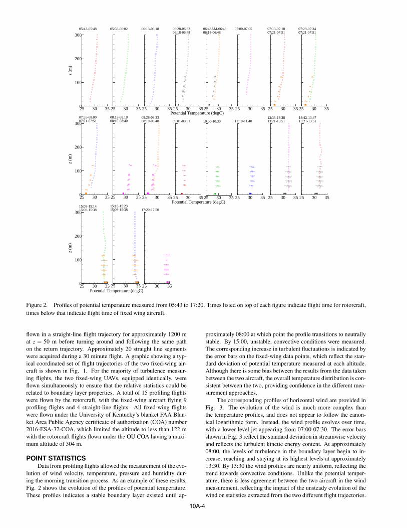
Figure 2. Profiles of potential temperature measured from 05:43 to 17:20. Times listed on top of each figure indicate flight time for rotorcraft,times below that indicate flight time of fixed wing aircraft.

flown in a straight-line flight trajectory for approximately 1200 mat z = 50 m before turning around and following the same pathon the return trajectory. Approximately 20 straight line segmentswere acquired during a 30 minute flight. A graphic showing a typ-ical coordinated set of flight trajectories of the two fixed-wing air-craft is shown in Fig. 1. For the majority of turbulence measur-ing flights, the two fixed-wing UAVs, equipped identically, wereflown simultaneously to ensure that the relative statistics could berelated to boundary layer properties. A total of 15 profiling flightswere flown by the rotorcraft, with the fixed-wing aircraft flying 9profiling flights and 4 straight-line flights. All fixed-wing flightswere flown under the University of Kentucky’s blanket FAA Blan-ket Area Public Agency certificate of authorization (COA) number2016-ESA-32-COA, which limited the altitude to less than 122 mwith the rotorcraft flights flown under the OU COA having a maxi-mum altitude of 304 m.

POINT STATISTICSData from profiling flights allowed the measurement of the evo-

lution of wind velocity, temperature, pressure and humidity dur-ing the morning transition process. As an example of these results,Fig. 2 shows the evolution of the profiles of potential temperature.These profiles indicates a stable boundary layer existed until ap-

proximately 08:00 at which point the profile transitions to neutrallystable. By 15:00, unstable, convective conditions were measured.The corresponding increase in turbulent fluctuations is indicated bythe error bars on the fixed-wing data points, which reflect the stan-dard deviation of potential temperature measured at each altitude.Although there is some bias between the results from the data takenbetween the two aircraft, the overall temperature distribution is con-sistent between the two, providing confidence in the different mea-surement approaches.

The corresponding profiles of horizontal wind are provided inFig. 3. The evolution of the wind is much more complex thanthe temperature profiles, and does not appear to follow the canon-ical logarithmic form. Instead, the wind profile evolves over time,with a lower level jet appearing from 07:00-07:30. The error barsshown in Fig. 3 reflect the standard deviation in streamwise velocityand reflects the turbulent kinetic energy content. At approximately08:00, the levels of turbulence in the boundary layer begin to in-crease, reaching and staying at its highest levels at approximately13:30. By 13:30 the wind profiles are nearly uniform, reflecting thetrend towards convective conditions. Unlike the potential temper-ature, there is less agreement between the two aircraft in the windmeasurement, reflecting the impact of the unsteady evolution of thewind on statistics extracted from the two different flight trajectories.

10A-4

0 5

05:58-06:02

0 5

06:13-06:18

0 5

06:28-06:3206:18-06:48

0 5

06:43AM-06:4806:18-06:48

0 5

07:00-07:05

0 5

07:13-07:1807:21-07:51

0 5

07:29-07:3407:21-07:51

z(m

)

0 50

100

200

300

07:55-08:0007:21-07:51

0 5

08:13-08:1808:10-08:40

0 5

08:28-08:3308:10-08:40

0 5

09:01-09:31

0 5

10:00-10:30

0 5

11:10-11:40

0 5

13:33-13:3813:21-13:51

0 5

13:42-13:4713:21-13:51

z(m

)

0 50

100

200

300

15:09-15:1415:08-15:38

0 5

15:18-15:2315:08-15:38

0 5

17:20-17:50

z(m

)

0 50

100

200

300

05:43-05:48

Horizontal velocity magnitude (m/s)

Horizontal velocity magnitude (m/s)

Horizontal velocity magnitude (m/s)

Figure 3. Profiles of horizontal velocity magnitude measured from 05:43 to 17:20. Times listed on top of each figure indicate flight time forrotorcraft, times below that indicate flight time of fixed wing aircraft.

RELATIVE STATISTICSTo obtain relative statistics, data from the straight-line flight

path was used. To do this, the coordinate system was re-orientedto xi, in which i = 1 was the component in the flight direction andparallel to the ground, i = 2 was the horizontal component perpen-dicular to the flight direction and i = 3 was in the vertical direction.Typically, twenty passes of 1200 m were flown and each straightline segment of each pass was treated as a member of an ensemble,allowing calculation of ensemble-averaged statistics. To account forthe advection of the flow, Taylor’s hypothesis was applied wherebyfor each pass the mean wind velocity Ui was calculated for eachmember of the ensemble and a second coordinate system was deter-mined such that x∗i = xi−Uit.

To calculate the auto-correlation, R11(r1), the mean windvelocity was first subtracted to find u1, then 〈u1(x1)u1(x1 +r1)〉/〈u1(x1)

2〉 was calculated where x1 indicates the location alongthe flight path, and r1 all possible separation distances. Here the 〈〉brackets indicate averaging over all values of x1 and for all membersof the ensemble. A similar process was used to calculate R22(r1)and R33(r1) with the calculation repeated for x∗i and r∗i . The result-ing correlations are provided in Fig. 4.

The correlations show the expected monotonic decrease with

increasing r1, although at higher values of r1 there is increasedscatter in the correlations due to decreased statistical convergence.As the boundary layer transitioned from neutrally stable towardsbeing convective, the region of correlation increased. As a result,the longitudinal integral scales, L11 =

∫R11dr1 increased from ap-

proximately 30 m to 90 m between 08:00 and 15:30. The increasein L11/z from 0.6 to 1.8 reflects the increased formation of long-wavelength structures. despite the increase in convective activityand proximity to the surface. The lateral scales increased as well,with L33 ≈ 0.5L11 and L22 ≈ 0.8L11. Note that, as shown in Figure4, there is no significant difference between the correlations calcu-lated in the xi and x∗i coordinate systems, suggesting that the correc-tion for advection had little impact on this statistic.

The longitudinal structure functions were also calculated usingSn = 〈[u1(x1)−u1(x1 + r1)]

n〉, following the same procedure as thecorrelations. Although the structure functions not presented heredue to space limitations, this calculation allowed the mean dissipa-tion rate, ε to be estimated from Kolmogorov’s 4/5 law by findingthe average value of ε =−1.2S3/r1 over a range of 0.5 m< r1 < 15m. In turn, the dissipation rate then allowed estimation of the Taylormicroscale Reynolds number, which was found to be Reλ ≈ 7×103,4×104, 5×104, and 5×104 for each of the four flights.

10A-4

r1 (m); r1* (m)

R22

0 100 200 300 400

0

0.5

1(b)

r1 (m); r1* (m)

R33

0 100 200 300 400

0

0.5

1(c)

r1 (m); r1* (m)

R11

0 100 200 300 400

0

0.5

108:07-08:3709:57:10:2711:06-11:3615:06:15:36

(a)

Figure 4. Autocorrelations (a) R11; (b) R22; and (c) R33 calculated for each flight. Dotted lines indicate values calculated from the xi coordinatesystem and solid lines indicate the values calculated from the x∗i coordinate system.

Having an estimate of the dissipation rate also allowed calcu-lation of the Kolmogorov scale η = (ν3/ε)1/4, and thus allowedKolmogorov scaling of the wavenumber spectra, which are shownin Fig. 5. To calculate these spectra, the wavenumber was estimatedas k1 = 2π/r1. The spectra calculated from each flight leg werethen ensemble-averaged to produce the resulting one-dimensionalwavenumber spectra E11(k1), E22(k1), E33(k1) for all three compo-nents of velocity. Also shown in Fig. 5 are the same spectra calcu-lated in the x∗i coordinate system. The results show little differencebetween spectra calculated with an assumed advection and with-out assuming advection of the flow field, but do reveal two to threedecades of inertial subrange range having a k−5/3

1 decay. Note thatthe decay observed in Fig. 5 at the highest wavenumbers presenteddoes not reflect dissipation, but is instead the filtering introduced bythe five-hole probe due to its limited frequency response.

The roll-off in the inertial subrange is emphasized in the com-pensated spectra shown in Figure 6. The expected broadening of theinertial subrange with increasing Reynolds number becomes read-ily apparent. Although the lower wavenumbers show evidence ofincomplete statistical convergence, the higher wavenumbers are inbroad agreement with Kolmogorov’s constants, indicated by dashedlines. These compensated spectra suggested that at the lowest Reλ ,most of the energy containing eddy range was captured by the 1200m flight path. However, as Reλ increased, the low wavenumberrange became increasingly less resolved.

ConclusionsThe results presented here demonstrate that it is possible to

obtain high-Reynolds-number turbulence data in the atmosphericboundary layer using unmanned aerial vehicles. As these vehiclesare traveling at velocities an order of magnitude faster than the windvelocity, the statistics are effectively being measured in space, ratherthan time. This is illustrated in the reduced impact of Taylor’s hy-pothesis on the statistics, which manifests in only minor differencesat large separations. Limitations in the approach of using UAVs ap-pears as decreased statistical convergence at longer separation dis-tances, and through the limited frequency response of the five-holeprobe. Improvements are currently being made in the measurementsystem to improve these qualities.

During the measurements, which were conducted during amorning transition from stable to unstable conditions, autocorrela-tions, structure functions, and spectra were successfully measured.These results showed that during this period, at z = 50 m, the Tay-lor microscale Reynolds number increased by an order of magni-tude from Reλ ≈ 7× 103 to 5× 104 and the longitudinal integralscales increased from 30 m to 90 m. The spectra measured over thisperiod showed an order of magnitude increase in the wavenumberrange of the inertial subrange, with the subrange constants in roughagreement with the Kolmogorov predictions.

AcknowledgmentsThis work was supported by the National Science Foundation

through grant #CBET-1351411 and by National Science Foundationaward #1539070, Collaboration Leading Operational UAS Devel-opment for Meteorology and Atmospheric Physics (CLOUDMAP).The authors would like to thank Ryan Nolin, Caleb Canter, JonathanHamilton, Elizabeth Pillar-Little, William Sanders, and Robert Sin-gler who worked tirelessly to build, maintain, and fly the unmannedvehicles used in this study.

REFERENCESdel Alamo, J.C. & Jimenez, J. 2009 Estimation fo turbulent convec-

tion velocities and corrections to taylor’s approximation. J. FluidMech. 640, 5–26.

Dhanak, M.R. & Holappa, K. 1999 An autonomus ocean turbulencemeasurement platform. Journal of Atmospheric and OceanicTechnology 16, 1506–1518.

Eberhard, W.L., Cupp, R.E. & Healey, K.R. 1989 Doppler lidarmeasurement of profiles of turbulence and momentum flux. J.Atmos. Oceanic Technol. 6, 809–819.

Eheim, C., Dixon, C., Agrow, B.M. & Palo, S. 2002 Tornadochaser: A remotely-piloted UAV for in situ meteorological mea-surements. In AIAA Paper 2002-3479, 1st AIAA UnmannedAerospace Vehicles, Systems, Technologies, and Operations Con-ference and Workshop.

Grant, H. L., Stewart, R. W. & Moilliet, A. 1962 Turbulence spectrafrom a tidal channel. J. Fluid Mech. 12, 241–268.

Guala, M., Metzger, M. & McKeon, B. 2011 Interactions withinthe turbulent boundary layer at high Reynolds number. J. FluidMech. 666, 573–604.

Higgins, C.W., Froidevaux, M., Simeonov, V., Vercauteren, N.,Barry, C. & Parlange, M.B. 2012 The effect of scale on theapplicability of taylors frozen turbulence hypothesis in the at-mospheric boundary layer. Boundary-Layer Meteorol. 143, 379–391.

van den Kroonenberg, A., Martin, T., Buschmann, M., Bange, J.& Vorsmann, P. 2008 Measuring the wind vector using the au-tonomous mini aerial vehicle M2AV. J. Atmos. Oceanic Technol.25, 1969–1982.

Lenschow, D.H. & Johnson, W.B. 1968 Concurrent airplane andballoon measurments of atmospheric boundary layer structureover a forest. J. Appl. Meteor. 7, 79–89.

Levine, E. R. & Lueck, R.G. 1999 Turbulence measurements froman autonomous underwater vehicle. Journal of Atmospheric andOceanic Technology 16, 1533–1544.

Matvev, V., Dayan, U., Tass, I. & Peleg, M. 2002 Atmospheric sul-fur flux rates to and from israel. The Science of the Total Envi-ronment 291, 143–154.

Mayer, S, Jonassen, M, Sandvik, A & Reuder, J 2012 Atmosphericprofiling with the UAS SUMO: a new perspective for the evalu-

10A-4

k1; k1*

E11

/(

5 )1/4

10-6 10-5 10-4 10-3 10-2 10-1101

102

103

104

105

106

107

108

109

08:07-08:3709:57-10:3711:06-11:3615:06-15:36

(a)

k1; k1*

E22

/(

5 )1/4

10-6 10-5 10-4 10-3 10-2 10-1101

102

103

104

105

106

107

108

109(b)

k1; k1*

E33

/(

5 )1/4

10-6 10-5 10-4 10-3 10-2 10-1101

102

103

104

105

106

107

108

109(c)

Figure 5. Scaled power spectra (a) E11(k1); (b) E22(k1); and (c) E33(k1) calculated for each flight. Dotted lines indicate values calculatedfrom the xi coordinate system and solid lines indicate the values calculated from the x∗i coordinate system.

k1; k1*

-2/3k 15/

3 E11

10-6 10-5 10-4 10-3 10-2 10-10

0.2

0.4

0.6

0.8

108:07-08:3709:57-10:3711:06-11:3615:06-15:36

(a)

k1; k1*

-2/3k 15/

3 E22

10-6 10-5 10-4 10-3 10-2 10-10

0.2

0.4

0.6

0.8

1(b)

k1; k1*

-2/3k 15/

3 E33

10-6 10-5 10-4 10-3 10-2 10-10

0.2

0.4

0.6

0.8

1(c)

Figure 6. Compensated power spectra (a) E11(k1); (b) E22(k1); and (c) E33(k1) calculated for each flight. Dotted lines indicate valuescalculated from the xi coordinate system and solid lines indicate the values calculated from the x∗i coordinate system.

ation of fine-scale atmospheric models. Meteorology and Atmo-spheric Physics 116 (1–2), 15–26.

Metzger, M. & Holmes, H. 2008 Time scales in the unstable atmo-spheric surface layer. Boundary-Layer Meteorol. 126, 29–50.

Metzger, S., Junkermann, W., Butterbach-Bahl, K., Schmid, H. P.& Foken, T. 2011 Measuring the 3-d wind vector with a weight-shiftmicrolight aircraft. Atmos. Meas. Tech. 4, 1421–1444.

Monty, J.P., Hutchins, N., Ng, H.C.H., Marusic, I. & Chong, M.S.2009 A comparison of turbulent pipe, channel and boundarylayer flows. J. Fluid Mech. 632, 431–442.

Neumann, P. P. & Bartholmai, M. 2015 Real-time wind estimationon a micro unmanned aerial vehicle using its internal measure-ment unit. Sensors and Actuators A: Physical 235, 300310.

Palomaki, Ross T., Rose, Nathan T., van den Bossche, Michael,Sherman, Thomas J. & Wekker, Stephan F.J. De 2017 Wind esti-mation in the lower atmosphere using multi-rotor aircraft. Jour-nal of Atmospheric and Oceanic Technology Early online re-lease.

Payne, F.R. & Lumley, J.L. 1966 One-dimensional spectra derived

from an airborne hot-wire anemometer. Quarterly Journal of theRoyal Meteorological Society 92, 397–401.

Philbrick, C.R. 2002 Raman lidar descriptions of lower atmosphereprocesses. In Proceedings of the 21st ILRC, Valcartier, QuebecCanada, p. 535545.

Sheih, C. M., Tennekes, H. & Lumley, J.L. 1971 Airborne hot-wiremeasurements of the small-scale structure of atmospheric turbu-lence. Phys. Fluids 14 (2), 201–215.

Taylor, G. I. 1938 The spectrum of turbulence. Proc. R. Soc. Lond.164 (919), 476–490.

Thorpe, S. A., Osborn, T. R., Jackson, J. F. E., Hall, J. & Lueck,R. G. 2003 Measurements of turbulence in the upper-ocean mix-ing layer using Autosub. Journal of Physical Oceanography 33,122–145.

Trevino, G. & Andreas, E.L. 2008 On reynolds averaging of turbu-lence time series. Boundary-Layer Meteorol. 128, 303–311.

Zaman, K.B.M.Q & Hussain, A.K.M.F 1981 Taylor hypothesis andlarge-scale coherent structures. J. Fluid Mech. 112, 379–396.

10A-4