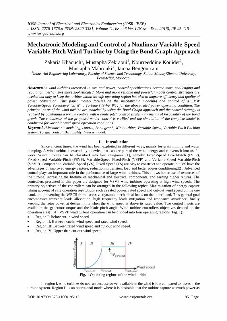
Mechatronic Modeling and Control of a Nonlinear Variable … Issue 6/Version-1... · The bond graph...

IOSR Journal of Electrical and Electronics Engineering (IOSR-JEEE)

e-ISSN: 2278-1676,p-ISSN: 2320-3331, Volume 11, Issue 6 Ver. I (Nov. – Dec. 2016), PP 95-115

www.iosrjournals.org

DOI: 10.9790/1676-11060195115 www.iosrjournals.org 95 | Page

Mechatronic Modeling and Control of a Nonlinear Variable-Speed

Variable-Pitch Wind Turbine by Using the Bond Graph Approach

Zakaria Khaouch1, Mustapha Zekraoui

1, Nourreeddine Kouider

1,

Mustapha Mabrouki1 , Jamaa Bengourram

,1Industrial Engineering Laboratory, Faculty of Science and Technology, Sultan MoulaySlimane University,

BeniMellal, Morocco.

Abstract:As wind turbines increased in size and power, control specifications became more challenging and

regulation mechanisms more sophisticated. More and more reliable and powerful model control strategies are

needed not only to keep the turbine within its safe operating region but also to improve efficiency and quality of

power conversion. This paper mainly focuses on the mechatronic modeling and control of a 5MW

Variable-Speed Variable-Pitch Wind Turbine (VS-VP WT) for the above-rated power operating condition. The

principal parts of the wind turbine are modeled by using the Bond-Graph approach and the control strategy is

realized by combining a torque control with a blade pitch control strategy by means of bicausality of the bond

graph. The robustness of the proposed model control is verified and the simulation of the complete model is

conducted for variable wind speed operation conditions.

Keywords:Mechatronic modeling, control, Bond graph, Wind turbine, Variable-Speed, Variable-Pitch Pitching

system, Torque control, Bicausality, Inverse model.

I. Introduction

Since ancient times, the wind has been exploited in different ways, mainly for grain milling and water

pumping. A wind turbine is essentially a device that capture part of the wind energy and converts it into useful

work. Wind turbines can be classified into four categories [1], namely: Fixed-Speed Fixed-Pitch (FSFP),

Fixed-Speed Variable-Pitch (FSVP), Variable-Speed Fixed-Pitch (VSFP) and Variable-Speed Variable-Pitch

(VSVP). Compared to Variable-Speed (VS), Fixed-Speed (FS) are easy to construct and operate, but VS have the

advantages of improved energy capture, reduction in transient load and better power conditioning[2]. Advanced

control plays an important role in the performance of large wind turbines. This allows better use of resources of

the turbine, increasing the lifetime of mechanical and electrical components, and earning higher returns. The

controllers presented in this paper are designed for VSVP wind turbines operating at high wind speeds. The

primary objectives of the controllers can be arranged in the following topics: Maximization of energy capture

taking account of safe operation restrictions such as rated power, rated speed and cut-out wind speed on the one

hand, and preventing the WECS from excessive dynamic mechanical loads on the other hand. This general goal

encompasses transient loads alleviation, high frequency loads mitigation and resonance avoidance, finally

keeping the rotor power at design limits when the wind speed is above its rated value. Two control inputs are

available: the generator torque and the blade pitch angle. Wind turbine controllers objectives depend on the

operation area[3, 4]. VSVP wind turbine operation can be divided into four operating regions (Fig. 1):

Region I: Below cut-in wind speed.

Region II: Between cut-in wind speed and rated wind speed.

Region III: Between rated wind speed and cut-out wind speed.

Region IV: Upper than cut-out wind speed.

Fig. 1 Operating regions of the wind turbine

In region I, wind turbines do not run because power available in the wind is low compared to losses in the

turbine system. Region II is an operational mode where it is desirable that the turbine capture as much power as

Mechatronic Modeling and Control of a Nonlinear Variable-Speed Variable-Pitch Wind…


possible from the wind, this is due to the fact that wind energy extraction rates are low and the structural loads are

relatively small. The generator torque provides the control input to vary the rotor speed, while the blade pitch is

held constant. Region III is encountered when the wind speeds are high enough; then the turbine must limit the

fraction of the captured wind power such that safe electrical and mechanical loads are not exceeded. If wind

speeds exceed contains the region III (region IV), the system will make a forced stop of the machine, protecting it

from excessively high aerodynamic loads. In practice, the passage from region II to region III is somewhat

unusual. In fact, the electromagnetic torque in region II controls the rotor speed, and in region III it is the power

that should be controlled by the blade pitch control.

Many works have proposed controllers to work around an operating point using control of the generator

torque to keep the turbine at a condition of maximum power point tracking, e.g., [5]. Some previously published

works proposed pitch control methods to limit the rotor speed at high wind speeds, e.g., [6]. In [7] a combination

of proportional integral (PI) and SMC is used to adjust the turbine rotor speed for extracting maximum power

without estimating the wind speed. In [8] a PI based torque control is used to control the WT, where optimal gains

are achieved by particle swarm optimization and fuzzy logic theory, [9]discussed the multivariable control

strategy by combining the nonlinear state feedback control for region II with linear control for region III. Finally,

the results are compared with the existing control strategies such as PID and LQG. WT control using adaptive

radial basic NN used for both pitch and torque controllers is addressed in [10]. Active disturbance rejection based

pitch control for variable speed WT is presented in [11]. Relatively few works suggest control strategies based on

varying operating conditions for wind turbines and their dynamics and using a unified approach in modeling and

control of the wind turbine. The principal aim of this paper is to show same benefits of the bond graph in modeling

and control of the wind turbine. In this subject, a wind turbine mechatronic model is developed. The main

components of the system are modeled using the Bond-Graph Approach (BGA). The control law is derived by

combining a torque control strategy with a pitch control by using the inverse model of the bond graph; a

compression with a PID controller is done to validate the propos model control. The implementation of the

complete model and its control system has been carried out by means of the 20-Sim simulation program.

The paper is organized as follows. Section 2 discusses the modeling of the WT by using the BGA.

Problem formulation and control objectives are discussed in Section 3. The proposed controllers for all the regions

are discussed in Section 4. Section 5 discusses the validation of the results using the 20-Sim simulator. Finally in

Section 6 a conclusion is drawn from the obtained results, which show that the proposed bond graph model control

is working fine for controlling the WT at below and above rated wind speeds.

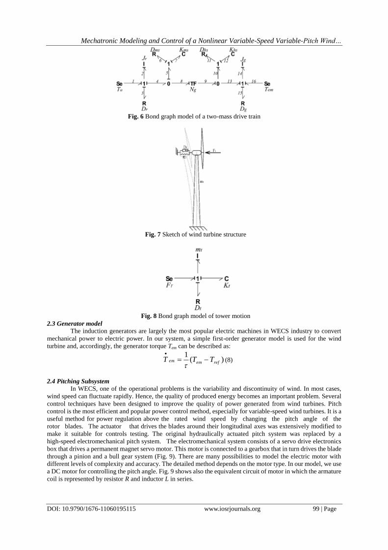
II. System modeling of the wind turbine by using the Bond graph Approach (BGA) The wind turbine studied in this paper is a 5 MW horizontal axis and is a variable speed variable pitch

wind turbine. The specifications of this turbine are described in [12] and some of its parameters are shown in

Appendix A. Based on it, the mechatronic model of the wind energy conversion systems (WECS) can be stated,

and the main components of a WECS will be presented by using the bond graph approach (BGA). Our primary

objective is to show some of the benefits of the BGA in contributing to a model of wind turbine and presenting a

nonlinear model of a wind turbine in a unified framework, containing aerodynamic system, drive train, tower,

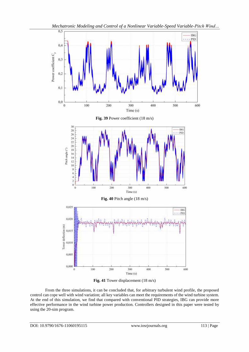
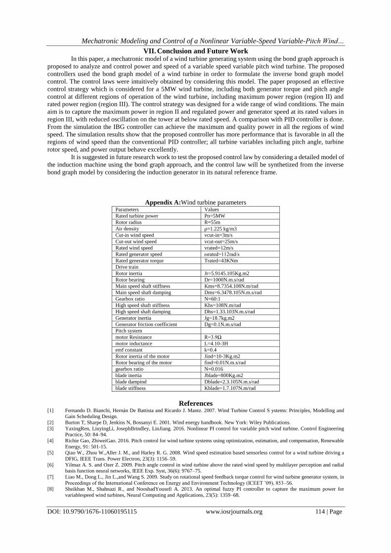
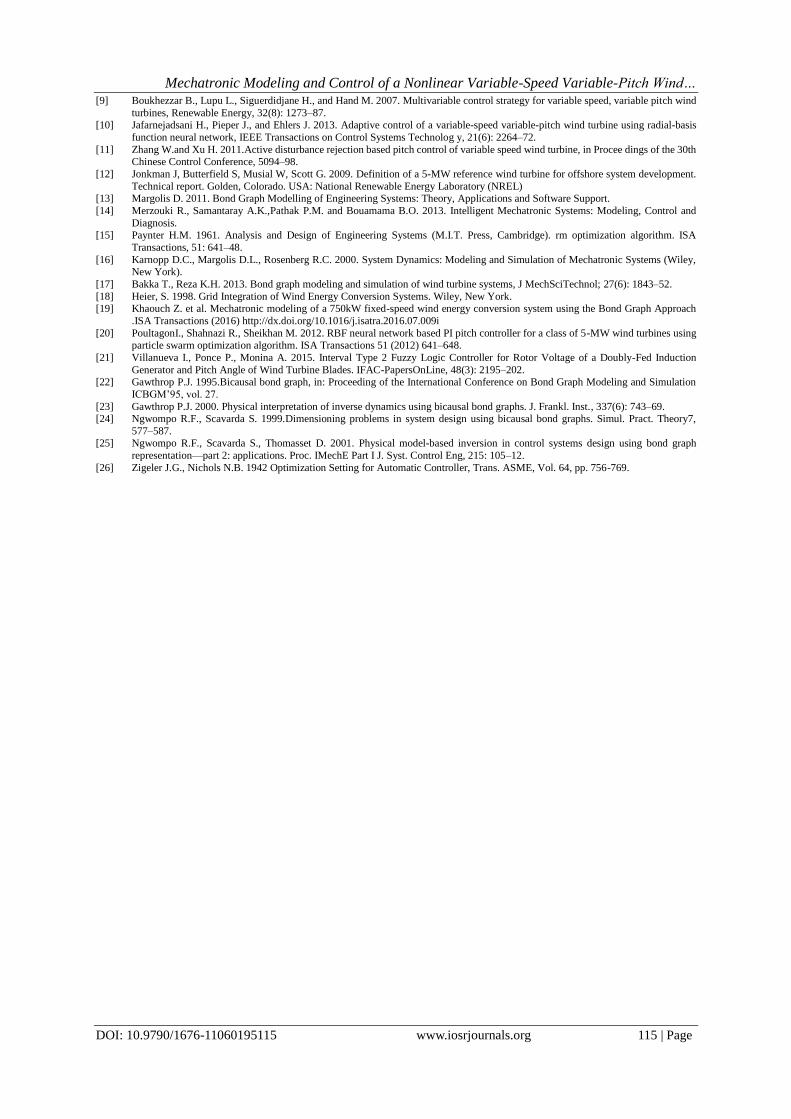
generator and pitching system.

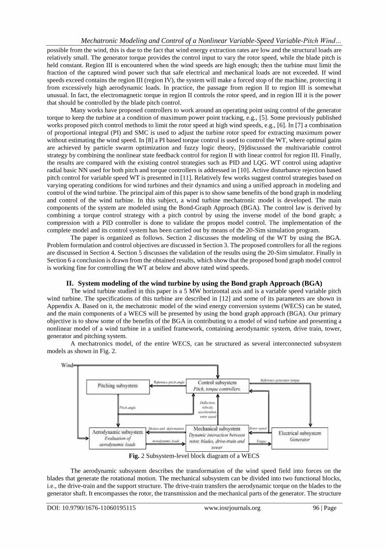
A mechatronics model, of the entire WECS, can be structured as several interconnected subsystem

models as shown in Fig. 2.

Fig. 2 Subsystem-level block diagram of a WECS

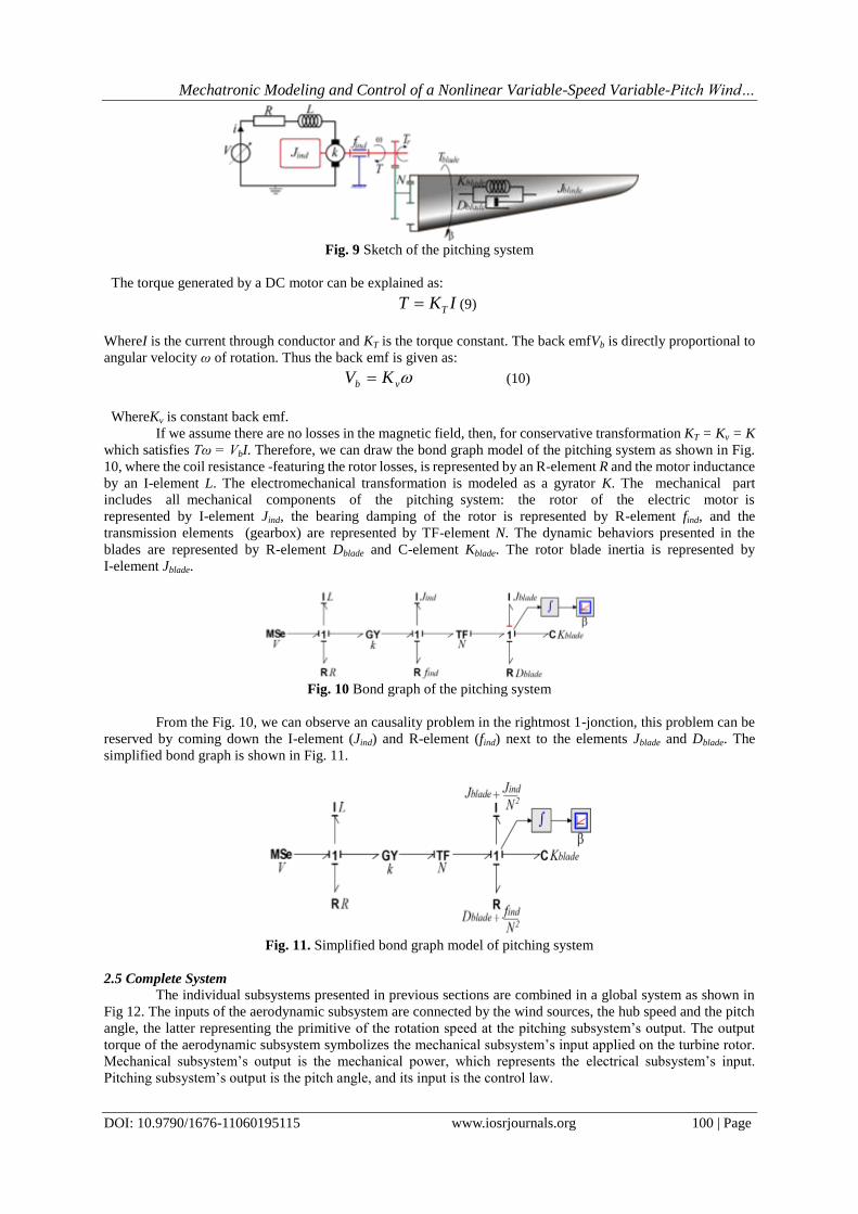
The aerodynamic subsystem describes the transformation of the wind speed field into forces on the

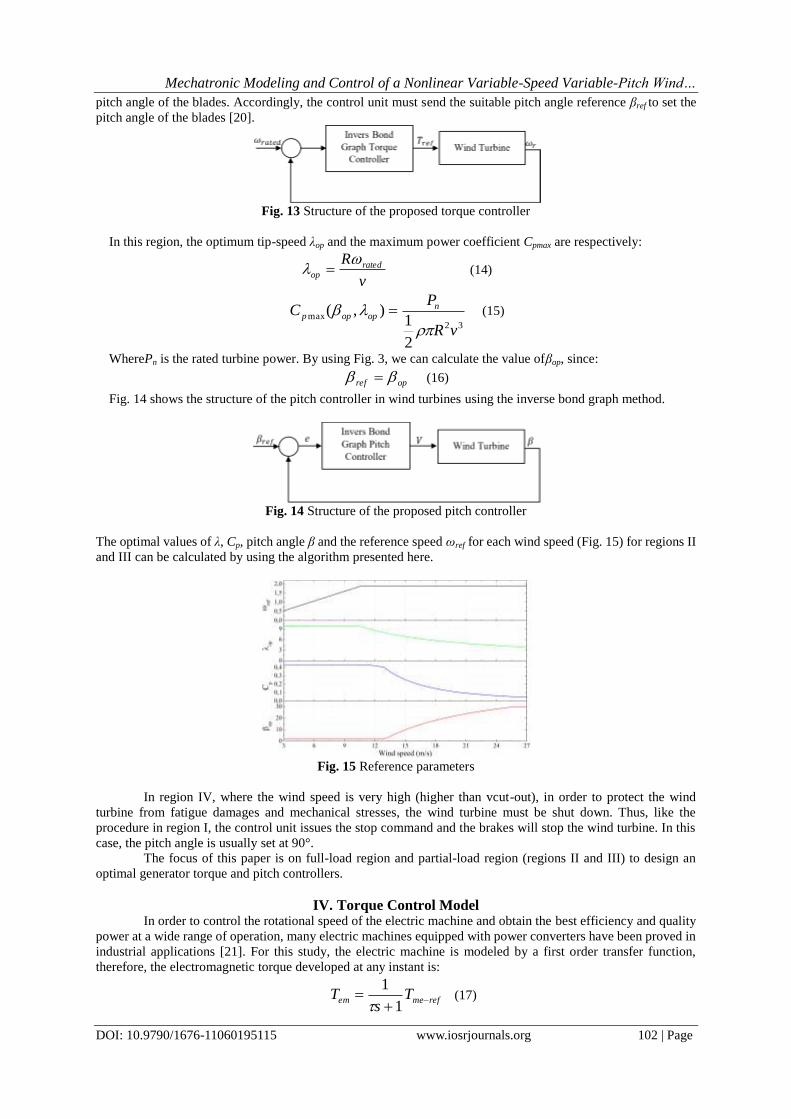
blades that generate the rotational motion. The mechanical subsystem can be divided into two functional blocks,

i.e., the drive-train and the support structure. The drive-train transfers the aerodynamic torque on the blades to the

generator shaft. It encompasses the rotor, the transmission and the mechanical parts of the generator. The structure



is made up of the tower. The electrical subsystem describes the conversion of mechanical power at the generator

shaft into electricity. Finally, the actuator subsystem models the pitch servo behavior. In order to analyze the

system in the same reference frame, the BGA [13, 14] is used.

The bond graph is a graphical way of modeling the analysis and control of multidisciplinary systems

(independent of the physical nature of the studied system), precisely due to its graphical nature of displaying the

power exchange in a system, which includes storage, dissipation and transformation. Paynter, the inventor of bond

graphs [15], published his first book in 1959. Karnopp et al. later extended the approach in [16], where the

presentation starts with the basic elements and leads to sophisticated mathematical models suitable for automated

computer simulation.

2.1 Aerodynamics bond graph model

The wind turbine rotor transforms the absorbed kinetic energy of the air into mechanical power. The power in the

wind is proportional to the cube of the wind speed and can be described as[17]:

32

2

1vRPwind (1)

Where is air density, R is rotor radius of the wind turbine blade, and v is wind speed. A wind turbine can

only extract part of the power from the wind. The ratio of the power Cp(β,λ) extracted from the wind is a nonlinear

function of the blade pitch angle β and the tip-Speed Ratio λ. Therefore, the mechanical power of the wind turbine

extracted from the wind can be expressed as [17]:

),(2

1 32 pmech CvRP (2)

With:

v

R r (3)

Whereωr is the speed of the turbine rotor. From (2) we can find the aerodynamic torque and the thrust

force acting on the tower:

),(2

1 32 qa CvRT (4)

),(2

1 22 TT CvRF (5)

WhereCq(β,λ) is the torque coefficient given as:

),(),(

pCCq and CT(β,λ) is the thrust force

coefficient. A generic equations is used to model Cp(β,λ) and CT(β,λ). These equations are based on the modeling

turbine characteristics of [18]. The power coefficient used in the calculation of the torque is given in (6). A plot of

the Cp(β,λ) curve is shown in Fig. 3; the plot is made with different pitch angle and tip-speed ratio. Similar

formulas can be found regarding the thrust force coefficient CT(β,λ); in our calculations only a simple relation is

used:

6432

1

5

)(),( ceccc

cC i

c

i

p

(6)

1

035.0

08.0

1

1

2

i(7)

Where :c1=0.5179, c2=116, c3=0.4, c4=5, c5=21 and c6=0.0068.

In the aerodynamics part, we need to find a way to convert the wind into torque and thrust force, i.e. to

transform a flow into efforts. This is done by means of a modulated gyrator MGY. We use the torque and thrust

force equations given in (4) and (5). In this case the transformation is dependent on three varying parameters: the

wind speed v, the pitch angle β, and the rotor rotational speed ωr. Fig. 4 shows the bond graph model of the

aerodynamics part.



Fig. 3 Curve of Cp

Fig. 4 Bond graph model of the aerodynamics part

2.2 Mechanical subsystem model

The mechanical subsystem includes all mechanical components of the wind turbine system; it can be

divided in two flexible structures, the drive train and the tower. In this system, the rotor of the turbine, the

transmission elements (gearbox) and the rotor generator composes the drive train. This can be modeled as a

multi-body system (MBS) with multiple degrees of freedom. Fig. 5 shows, a sketch of a two-mass drive train

model, a more detailed bond graph model is presented in [19]. The bond graph representation of the drive train is

shown in Fig. 6. The model consists of two 1-junctions and two 0-junctions. The rightmost 1-junction connected

to the rotor inertia Jr and rotor external damping Dr describes the rotor rotational speed ωr. Since there are

dynamics in between the rotor inertia and the generator inertia, they do not have the same speed. This is the reason

for the 0-junction in the main and high speed. The 1-junction connected to the R-element (Dms, Dhs) and the

C-element (kms, Khs) describe respectively the damping and stiffness in the main and high-speed shafts; the

gearbox is modeled by a simple TF-element where (Ng) is the gearbox ratio, the generator inertia (Jg) and external

damping (Dg) are respectively modeled by the I-element and the R-element.

Fig. 5 Sketch of a two-mass drive train

For the tower model it is assumed that the tower moves only in horizontal direction (Fig. 7) and does not

influence the mechanical system; it only affects its input, i.e. the wind speed. The bond graph model of the tower

is sketched in Fig. 8, where mt is the tower mass, Ft is the thrust force acting on the tower,Dt is the tower damping

and Kt is the tower stiffness.



Fig. 6 Bond graph model of a two-mass drive train

Fig. 7 Sketch of wind turbine structure

Fig. 8 Bond graph model of tower motion

2.3 Generator model

The induction generators are largely the most popular electric machines in WECS industry to convert

mechanical power to electric power. In our system, a simple first-order generator model is used for the wind

turbine and, accordingly, the generator torque Tem can be described as:

)(1

refemem TTT

(8)

2.4 Pitching Subsystem

In WECS, one of the operational problems is the variability and discontinuity of wind. In most cases,

wind speed can fluctuate rapidly. Hence, the quality of produced energy becomes an important problem. Several

control techniques have been designed to improve the quality of power generated from wind turbines. Pitch

control is the most efficient and popular power control method, especially for variable-speed wind turbines. It is a

useful method for power regulation above the rated wind speed by changing the pitch angle of the

rotor blades. The actuator that drives the blades around their longitudinal axes was extensively modified to

make it suitable for controls testing. The original hydraulically actuated pitch system was replaced by a

high-speed electromechanical pitch system. The electromechanical system consists of a servo drive electronics

box that drives a permanent magnet servo motor. This motor is connected to a gearbox that in turn drives the blade

through a pinion and a bull gear system (Fig. 9). There are many possibilities to model the electric motor with

different levels of complexity and accuracy. The detailed method depends on the motor type. In our model, we use

a DC motor for controlling the pitch angle. Fig. 9 shows also the equivalent circuit of motor in which the armature

coil is represented by resistor R and inductor L in series.



Fig. 9 Sketch of the pitching system

The torque generated by a DC motor can be explained as:

IKT T (9)

WhereI is the current through conductor and KT is the torque constant. The back emfVb is directly proportional to

angular velocity ω of rotation. Thus the back emf is given as:

vb KV (10)

WhereKv is constant back emf.

If we assume there are no losses in the magnetic field, then, for conservative transformation KT = Kv = K

which satisfies Tω = VbI. Therefore, we can draw the bond graph model of the pitching system as shown in Fig.

10, where the coil resistance -featuring the rotor losses, is represented by an R-element R and the motor inductance

by an I-element L. The electromechanical transformation is modeled as a gyrator K. The mechanical part

includes all mechanical components of the pitching system: the rotor of the electric motor is

represented by I-element Jind, the bearing damping of the rotor is represented by R-element find, and the

transmission elements (gearbox) are represented by TF-element N. The dynamic behaviors presented in the

blades are represented by R-element Dblade and C-element Kblade. The rotor blade inertia is represented by

I-element Jblade.

Fig. 10 Bond graph of the pitching system

From the Fig. 10, we can observe an causality problem in the rightmost 1-jonction, this problem can be

reserved by coming down the I-element (Jind) and R-element (find) next to the elements Jblade and Dblade. The

simplified bond graph is shown in Fig. 11.

Fig. 11. Simplified bond graph model of pitching system

2.5 Complete System

The individual subsystems presented in previous sections are combined in a global system as shown in

Fig 12. The inputs of the aerodynamic subsystem are connected by the wind sources, the hub speed and the pitch

angle, the latter representing the primitive of the rotation speed at the pitching subsystem’s output. The output

torque of the aerodynamic subsystem symbolizes the mechanical subsystem’s input applied on the turbine rotor.

Mechanical subsystem’s output is the mechanical power, which represents the electrical subsystem’s input.

Pitching subsystem’s output is the pitch angle, and its input is the control law.

IOSR Journal of Electrical and Electronics Engineering (IOSR-JEEE)

e-ISSN: 2278-1676,p-ISSN: 2320-3331, Volume 11, Issue 6 Ver. I (Nov. – Dec. 2016), PP 95-115

www.iosrjournals.org

DOI: 10.9790/1676-11060195115 www.iosrjournals.org 101 |

Page

Fig. 12 Complete System

III. Selection of the Operating Point Selection of the operating point is critical to preserving aerodynamic stability in the wind turbine system.

The rotational speed ωref operating point and the blade-pitch βref operating point were selected for each wind

speed using the following algorithms.

A wind turbine normally works in different operating modes along the wind speed range. It can be

divided into four regions shown in Fig. 1. The wind speeds; considered as the limits of this division, include cut-in

wind speed vcut-in, rated wind speed vrated and cut-out wind speed vcut-out[20]. The values of the 5MW wind turbine

studied in this paper are presented in appendix A. The control objectives in these regions are substantially

different.

Being below cut-in wind speed vcut-in (region I), the wind turbine power generation is very low and hence

not economical. Thus, the control unit shown in Fig. 2 issues the stop command and the brakes will stop the wind

turbine. In this region, the pitch angle is usually set at 90°[20].

In region II, which is called the partial-load region, the wind speed is higher than vcut-inbut lower than

vrated; the objective is to capture as much energy as possible. In this case, the power coefficient Cp should be set to

maximum power coefficient Cpmax. This occurs when both the tip-speed ratio λ and the pitch angle β are

maintained as close as possible to their optimum values λop and βop, since Cpmax = Cp(λop,βop). In Fig. 3, the

maximum Cp value over the entire surface occurs at a pitch angle of 2° and a tip-speed ratio of 9; the rotational

speed operating point ωop for each wind speed in this region is:

vR

op

op

(11)

When the generator speed does not exceed the rated generator speed, the reference speed is:

opref (12)

Moreover, when the generator speed exceeds the rated generator speed, the reference speed is:

ratedref (13)

Therefore, the rotational speed is varied in proportion to the wind speed by properly controlling the

generator torque. Fig. 13 shows the structure of this generator torque control method in wind turbines using the

inverse bond graph method.

In region III, which is called the full-load region, the wind speed is higher than vrated but lower than the

vcut-out. The main control purpose in this region is to keep the generator power Pg around the nominal generator

power Pn, by keeping the generator speed ωg around its rated value ωg-rated. This is achieved through tuning the



pitch angle of the blades. Accordingly, the control unit must send the suitable pitch angle reference βref to set the

pitch angle of the blades [20].

Fig. 13 Structure of the proposed torque controller

In this region, the optimum tip-speed λop and the maximum power coefficient Cpmax are respectively:

v

R ratedop

(14)

32max

2

1),(

vR

PC n

opopp

(15)

WherePn is the rated turbine power. By using Fig. 3, we can calculate the value ofβop, since:

opref (16)

Fig. 14 shows the structure of the pitch controller in wind turbines using the inverse bond graph method.

Fig. 14 Structure of the proposed pitch controller

The optimal values of λ, Cp, pitch angle β and the reference speed ωref for each wind speed (Fig. 15) for regions II

and III can be calculated by using the algorithm presented here.

Fig. 15 Reference parameters

In region IV, where the wind speed is very high (higher than vcut-out), in order to protect the wind

turbine from fatigue damages and mechanical stresses, the wind turbine must be shut down. Thus, like the

procedure in region I, the control unit issues the stop command and the brakes will stop the wind turbine. In this

case, the pitch angle is usually set at 90°.

The focus of this paper is on full-load region and partial-load region (regions II and III) to design an

optimal generator torque and pitch controllers.

IV. Torque Control Model In order to control the rotational speed of the electric machine and obtain the best efficiency and quality

power at a wide range of operation, many electric machines equipped with power converters have been proved in

industrial applications [21]. For this study, the electric machine is modeled by a first order transfer function,

therefore, the electromagnetic torque developed at any instant is:

refmeem Ts

T

1

1

(17)



WhereTem is the electromagnetic torque, Tref is the reference torque, and τ is the time constant.

The maximum power extraction techniques allow determining the speed of the turbine that achieves maximum

power generated. For the 1-junction placed between bonds 13, 14, 15 and 16 of the bond graph presented in Fig. 6,

we can write:

15141613 eeee (18)

Where: e13 = Tmg: which is the mechanical torque from the gearbox, e16 = -Tem, e14 = Jg(dωg/dt), where Jg

is the inertia of the generator and ωg is the generator angular velocity and e15 = Dgωg, where Dg is the generator

external damping.

Since we can write:

emggmg

g

g TDTdt

dJ

(19)

It can be seen that the mechanical speed is influenced by the action of two torques: the mechanical torque

from the gearbox and the electromagnetic torque from the electric machine. The torque control structure presented

in this paper adjusts the electromagnetic torque to set the wind turbine speed at its rated speed. In order to control

the electromagnetic torque, it is necessary to generate the reference electromagnetic torque. To this aim, a specific

algorithm is designed, based on the bicausal bond graph [22] and the performance of the system is compared with

a conventional PID controller to validate it.

The inverse model corresponds to a re-organization of the equations where the input and output roles are

exchanged: inputs become outputs and vice versa [23]. The inverse model is created by imposing both effort and

flow information from the sensor and receiving both at the source. This procedure, where both informations can be

imposed on a bond, cannot be done through normal causality. This is why, the notion of bicausality[24, 25] is

introduced. Bicausality notation splits the causality assignment for the two factors of power, namely effort and

flow. By separating the causal strokes, it allows imposing two complementary informations at one end of a bond.

In the inverse model, the source element (Se or Sf) is replaced by a source sensor (SeSf) element [23, 24]

and the sensor element (De or Df) is replaced by a sensor source (DeDf) element. The difference between the

source sensor and the sensor source lies in the causality of the element: the source sensor element receives

information of both power variables, whereas the signal source element supplies both. The rule for bicausal 0

(1)-junction is that only one bond can bring effort (flow) information and other bonds can bring the flow (effort)

information. This means that at a bicausal junction, there must be one bond bringing in both effort and flow

information while there must be another bond taking out both effort and flow information. Thus, at every junction,

only two bonds must be bicausal (not more, not less).

To arrive at the inverse model, bicausality is propagated from the original sensor to the original source. In

the process, some internal bonds in the model are assigned bicausality such that it is propagated to the receiving

source sensor.

The structure of the control in an open loop is designed with the inverse bond graph. The decoupling

actions are defined (inverse matrix and disturbance compensation). The open loop structure is then extended to a

closed loop control by fixing the dynamics of errors.

In our model, the input variable is the electromagnetic torque Tem and the output variable is the rotor

speed ωr of the turbine. The analysis of the direct bond graph model of Fig. 6 indicates that there is a power line

and a causal path between the input variable Tem and the output variable ωr. Therefore, the model is structurally

invertible compared to the pair of variables Tem and ωr. The objective of the controller established here is to

calculate the electromechanical torque required to set the turbine rotor speed to a reference. For this calculation, it

is appropriate to inverse the bond graph model of Fig. 6 relatively to the pair of variables Tem and ωr.

The inverse bond graph model of the system is given in Fig. 16; the sensor (Df) and source (Sf) have been

replaced with source sensor (SeSf) element and sensor source (DeDf) element. Note that fixed sources (those

which are not control inputs) are retained as they are, e.g., Se: Ta at bond number 1. The SeSf element in bond

number 0 imposes both effort and flow information, thereby forcing differential causality in the I-element at bond

number 2. Likewise, three more storage elements are forced to assume differential causality. The DeDf element at

bond number 16 receives both flow and effort information.



Fig. 16 Inverse bond graph for calculation of the controls laws.

From Fig.16, we can write the following from the constitutive relations of the leftmost 1-junction (i.e. 1-junction

placed between bonds 0, 1, 2, 3 and 4):

32014

43210

eeeee

fffff (20)

where: f0 = ωr, e0 = 0, e1 = Ta, e2 = Jr(dωr/dt) and e3=Drωr. Therefore:

rrr

ra

r

Ddt

dJTe

f

4

4

(21)

To establish the closed loop control law, the dynamics of the error are set in (22) as:

01 k (22)

Wherek1represents the controller to be used and ɛ=ωref- ωr, is the error. Expression (21) becomes (23) as:

rrrefra

r

DJTe

f

)(4

4

(23)

Finally,

rrrrefrrefra

r

DkJJTe

f

)(14

4

(24)

For the neighboring 0-junction in Fig. 15, we can write:

854

548

eee

fff(25)

From the 1-jonction between bonds 5, 6 and 7 we have:

765

765

eee

fff (26)

with:

dtfKdtfKe

fDfDe

msms

msms

577

566(27)

Therefore:

)(1

555 fDeK

f ms

ms

(28)

Proceeding in the same way, from the TF-element we can write:

g

g

N

ee

fNf

89

89

(29)

From the 0-junction placed between bonds 9, 10 and 13, we have:



13109

10913

eee

fff (30)

where:

)(1

101010 fDeK

f ms

ms

(31)

For the rightmost 1-junction, we can write:

15141316

1316

eeee

ff (32)

where:

e16 = -Tem, e14=Jg(dωg/dt), e15=Dgωg.

Finally:

ggggem DJeT

ff

9

1316 (33)

To generate the reference electromechanical torque the generator model must be inversed as:

ememrefem TTT (34)

The controller block diagram derived from these equations is shown in Fig. 17. It is important to notice

that the structure of the control law contains a feed-forward control with a derivative action. Fig. 17 shows that the

proposed gain is a PI controller; the estimate values are considered in the control law.

In the block diagram model, the desired output is the input. The output of the block diagram model is the

reference electromagnetic torque. The block diagram contains four derivative (d./dt) blocks. It was simulated for

the numerical parameters given in Appendix A.

V. Pitch Controller For the above rated wind speed the generator power is fixed to its rated value that is, maximum value of

the control input. In this condition, a linear pitch control is introduced. The blade pitch angle is adjusted to

maintain the generated power constant in its rated value. The form of the blades and, more generally, the turbine

characteristics play a key role in this power control.

Fig. 17 Torque control law block diagram

The non-linear model of the turbine makes complex to design an analytical model of this controller.

Moreover, very large differences (due to elasticity) may appear a turbine to another. That is why it is more

practical to use an experimental characteristic of the blade pitch angle measured for a different wind speed. The

inverse control characteristic can give directly for different wind speed the corresponding blade pitch angle; this is

achieved by using the algorithm given in section 3 and the controller should provide suitable motors voltage in its

output. This is obtained by using the inverse bond graph model of the pitching system.

The analysis of the bond graph model of Fig. 11 indicates that there is a power line and a causal path

between the input variable V and the output variable β. Therefore, the model is structurally invertible.

The inverse bond graph model of the pitching system is given in Fig. 18, as previously mentioned, the

sensor (Df) and source (Sf) have been replaced with source sensor (SeSf) elements. The SeSf element in bond

number 10 imposes both effort and flow information; the DeDf element at bond number 1 receives both flow and

effort information.

As previously defined in the torque controller, we can derive the equations from the inverse bond graph

of the Fig. 18.



Fig. 18 Inverse bond graph for calculation of the control law of the pitch system

From Fig. 18, we can write the following from the constitutive relations of the rightmost 1-junction (i.e.

1-junction placed between bonds 6, 7, 8, 9, and 10):

109876

109876

eeeee

fffff (35)

wheref10 = dβ/dt, e10 = 0, e9 = Kbladeβ, e8 = Deqv(dβ/dt) and e7 = Jeqv(d2β/dt

2). Therefore:

bladeeqveqv KDJe

f

6

6

(36)

To establish the closed loop control law of the pitch angle the dynamics of the error are set as (the controlled

variable is a generalized displacement):

032

kk

ref

(37)

Wherek2 and k3 represent the controllers to be used. Expression (36) becomes (48) as:

bladeeqv

refrefrefeqv

KD

kkJe

f

))()(( 326

6

(38)

From the TF-element and GY-element we can write:

65

65

NeeN

ff

(38)

54

54

keek

ef

(39)

Finally, for the leftmost 1-junction, we can write:

44321

4321

)()(

)(

)(

etRidt

tdiLeeetVe

tiffff

(40)

We can derive a block diagram model from the bicausalled bond graph model to control the pitch angle,

which is shown in Fig. 19. The proposed gains (k2 and k3) are PI controllers; the estimate values are considered in

the control law.

Fig. 19 Pitch control law block diagram



The bond graph representation of the complete system is shown in Fig. 20. The inputs to the systems are

pitch angle, reference parameters and wind speed. It can be seen that the wind turbine control system basically

contains two control loops, one is the pitch control loop and the other is the torque control loop. These two control

loops operate simultaneously, but only one of them is dominant depending on the operation region shown in Fig.

1. When the wind speed is below rated speed, the torque control loop is used to regulate the turbine speed to

capture maximal wind power. When the wind speed exceeds rated speed, the pitch control loop is used to provide

adequate pitch angle to regulate power at its rated value.

VI. Simulation and Discussion In order to verify the effectiveness and the robustness of the proposed control law, a simulation is carried

out by using different turbulent winds to drive the wind turbine, and a comparison between the proposed controller

and the conventional PI controller is done by considering these wind profiles. The PI parameters are generated

using Ziegler and Nichols methods [26].

Firstly, we consider the wind profile as shown in Fig. 21, secondly, we use a turbulent wind with mean

speed 12.5m/s and finally, the performance of the control system is tested during a turbulent wind with mean

speed 18m/s.

The wind speed profile as shown in Fig. 21 changes in step of every 20sec starting from 6m/s to 16m/s.

This shows that both the above and below rated wind speeds are included in the wind profile. For below rated wind

speed, the torque control comes into action with constant pitch angle, and for above rated wind speed, the pitch

control comes into action with rated power.

Fig. 22 shows the generator speed for the proposed method (inverse bond graph (IBG)) and PID

controller for below and above rated wind speeds. Both controllers achieve the nominal value of the generator

speed at 80sec. The corresponding wind speed is around 11m/s which can be seen from Fig. 21. As the wind speed

approaches the rated speed, the WT generator speed reaches the nominal value, that is, 112.35rad/s.Figs. 23 and

24 show respectively the electrical power and the power coefficient comparison for IBG and PID controllers for

the transition period. In region 2 IBG is able to extract more power than PID. Fig. 25 shows the generator torque

comparison in region 2 for IBM and PID. It can be observed that IBM produces more generated torque compared

to PID in region II. As the generator speed remains constant from 80sec onwards it is obvious that IBM captures

more power compared to PID. Fig. 26 shows the pitch angle comparison for PID and IBG; pitch variation is found

to be more for PID compared to IBG. Therefore, the pitch actuator needs more control action for PID. Fig. 27

shows the tower displacement comparison for PID and IBG. It can be observed that tower displacement in IBG is

less than PID controller.

Fig. 20 Bond graph model and its control system of the wind turbine



In order to create the appropriate conditions of comparing the two methods, the wind speed profile shown

in Fig. 28 with 12m/s average wind speed is used.

As is shown in Fig. 29, the turbine rotor speed remains around its rated value 112.35rad/s. Fig. 30 shows

the generator torque; in order to increase generator power, generator torque, generator speed or both must be

increased. Figs. 29 and 30 show that the generator speeds and torque in the proposed method are higher in

comparison with the conventional PID. Wind turbine power, shown in Fig. 31, reaches its rated value of 5MW.

Figs. 31 and 32 demonstrate that the proposed method is able to capture more electrical power in comparison with

the other controller. From Fig. 33, we find that the pitch system can track turbulent wind around cut-in speed.

Therefore, according to the simulation results, the proposed method has a more effective performance in the

generator torque control and pitch control in comparison with the conventional PID method; the tower

displacement in IBG is less than PID controller as shown in Fig. 34.

The control system performance is also tested during a turbulent wind with mean speed 18m/s, as shown

in Fig. 35. Turbine rotor speed, generator torque, power, power coefficient, pitch angle and tower displacement

are shown in Figs. 36 through 41 respectively. We can see that even for highly turbulent wind, all key turbine

variables behave excellently.

Fig. 21 Wind speed profile

Fig. 22 Generator speed

Fig. 23 Generator power



Fig. 24 Power coefficient

Fig. 25 Generator torque

Fig. 26 Pitch angle

Fig. 27 Tower displacement



Fig. 28 Wind speed profile (12m/s)

Fig. 29 Generator speed (12m/s)

Fig. 30 Generator torque (12m/s)

Fig. 31 Generator power (12m/s)



Fig. 32 Power coefficient (12m/s)

Fig. 33 Pitch angle (12m/s)

Fig. 34 Tower displacement (12m/s)

Fig. 35 Wind speed profile (18 m/s)



Fig. 36 Generator speed (18 m/s)

Fig. 37 Generator torque (18 m/s)

Fig. 38 Generator power (18 m/s)



Fig. 39 Power coefficient (18 m/s)

Fig. 40 Pitch angle (18 m/s)

Fig. 41 Tower displacement (18 m/s)

From the three simulations, it can be concluded that, for arbitrary turbulent wind profile, the proposed

control can cope well with wind variation; all key variables can meet the requirements of the wind turbine system.

At the end of this simulation, we find that compared with conventional PID strategies, IBG can provide more

effective performance in the wind turbine power production. Controllers designed in this paper were tested by

using the 20-sim program.



VII. Conclusion and Future Work In this paper, a mechatronic model of a wind turbine generating system using the bond graph approach is

proposed to analyze and control power and speed of a variable speed variable pitch wind turbine. The proposed

controllers used the bond graph model of a wind turbine in order to formulate the inverse bond graph model

control. The control laws were intuitively obtained by considering this model. The paper proposed an effective

control strategy which is considered for a 5MW wind turbine, including both generator torque and pitch angle

control at different regions of operation of the wind turbine, including maximum power region (region II) and

rated power region (region III). The control strategy was designed for a wide range of wind conditions. The main

aim is to capture the maximum power in region II and regulated power and generator speed at its rated values in

region III, with reduced oscillation on the tower at below rated speed. A comparison with PID controller is done.

From the simulation the IBG controller can achieve the maximum and quality power in all the regions of wind

speed. The simulation results show that the proposed controller has more performance that is favorable in all the

regions of wind speed than the conventional PID controller; all turbine variables including pitch angle, turbine

rotor speed, and power output behave excellently.

It is suggested in future research work to test the proposed control law by considering a detailed model of

the induction machine using the bond graph approach, and the control law will be synthetized from the inverse

bond graph model by considering the induction generator in its natural reference frame.

Appendix A:Wind turbine parameters Parameters Values

Rated turbine power Pn=5MW

Rotor radius R=55m

Air density =1.225 kg/m3

Cut-in wind speed vcut-in=3m/s

Cut-out wind speed vcut-out=25m/s

Rated wind speed vrated=12m/s

Rated generator speed ωrated=112rad/s

Rated generator torque Trated=43KNm

Drive train

Rotor inertia Jr=5.9145.105Kg.m2

Rotor bearing Dr=1000N.m.s/rad

Main speed shaft stiffness Kms=8.7354.108N.m/rad

Main speed shaft damping Dms=6.3478.105N.m.s/rad

Gearbox ratio N=60:1

High speed shaft stiffness Khs=108N.m/rad

High speed shaft damping Dhs=1.33.103N.m.s/rad

Generator inertia Jg=18.7kg.m2

Generator friction coefficient Dg=0.1N.m.s/rad

Pitch system

motor Resistance R=3.9Ω

motor inductance L=4.10-3H

emf constant k=0.4

Rotor inertia of the motor Jind=10-3Kg.m2

Rotor bearing of the motor find=0.01N.m.s/rad

gearbox ratio N=0.016

blade inertia Jblade=800Kg.m2

blade dampind Dblade=2.3.105N.m.s/rad

blade stiffness Kblade=1.7.107N.m/rad

References [1] Fernando D. Bianchi, Hernán De Battista and Ricardo J. Mantz. 2007. Wind Turbine Control S ystems: Principles, Modelling and

Gain Scheduling Design.

[2] Burton T, Sharpe D, Jenkins N, Bossanyi E. 2001. Wind energy handbook. New York: Wiley Publications.

[3] YaxingRen, LiuyingLi, JosephBrindley, LinJiang. 2016. Nonlinear PI control for variable pitch wind turbine. Control Engineering Practice, 50: 84–94.

[4] Richie Gao, ZhiweiGao. 2016. Pitch control for wind turbine systems using optimization, estimation, and compensation, Renewable

Energy, 91: 501-15. [5] Qiao W., Zhou W.,Aller J. M., and Harley R. G. 2008. Wind speed estimation based sensorless control for a wind turbine driving a

DFIG, IEEE Trans. Power Electron, 23(3): 1156–59.

[6] Yilmaz A. S. and Ozer Z. 2009. Pitch angle control in wind turbine above the rated wind speed by multilayer perception and radial basis function neural networks, IEEE Exp. Syst, 36(6): 9767–75.

[7] Liao M., Dong L., Jin L.,and Wang S. 2009. Study on rotational speed feedback torque control for wind turbine generator system, in

Proceedings of the International Conference on Energy and Environment Technology (ICEET ’09), 853–56. [8] Sheikhan M., Shahnazi R., and NooshadYousefi A. 2013. An optimal fuzzy PI controller to capture the maximum power for

variablespeed wind turbines, Neural Computing and Applications, 23(5): 1359–68.



[9] Boukhezzar B., Lupu L., Siguerdidjane H., and Hand M. 2007. Multivariable control strategy for variable speed, variable pitch wind

turbines, Renewable Energy, 32(8): 1273–87. [10] Jafarnejadsani H., Pieper J., and Ehlers J. 2013. Adaptive control of a variable-speed variable-pitch wind turbine using radial-basis

function neural network, IEEE Transactions on Control Systems Technolog y, 21(6): 2264–72.

[11] Zhang W.and Xu H. 2011.Active disturbance rejection based pitch control of variable speed wind turbine, in Procee dings of the 30th Chinese Control Conference, 5094–98.

[12] Jonkman J, Butterfield S, Musial W, Scott G. 2009. Definition of a 5-MW reference wind turbine for offshore system development.

Technical report. Golden, Colorado. USA: National Renewable Energy Laboratory (NREL) [13] Margolis D. 2011. Bond Graph Modelling of Engineering Systems: Theory, Applications and Software Support.

[14] Merzouki R., Samantaray A.K.,Pathak P.M. and Bouamama B.O. 2013. Intelligent Mechatronic Systems: Modeling, Control and

Diagnosis. [15] Paynter H.M. 1961. Analysis and Design of Engineering Systems (M.I.T. Press, Cambridge). rm optimization algorithm. ISA

Transactions, 51: 641–48.

[16] Karnopp D.C., Margolis D.L., Rosenberg R.C. 2000. System Dynamics: Modeling and Simulation of Mechatronic Systems (Wiley, New York).

[17] Bakka T., Reza K.H. 2013. Bond graph modeling and simulation of wind turbine systems, J MechSciTechnol; 27(6): 1843–52.

[18] Heier, S. 1998. Grid Integration of Wind Energy Conversion Systems. Wiley, New York. [19] Khaouch Z. et al. Mechatronic modeling of a 750kW fixed-speed wind energy conversion system using the Bond Graph Approach

.ISA Transactions (2016) http://dx.doi.org/10.1016/j.isatra.2016.07.009i

[20] PoultagonI., Shahnazi R., Sheikhan M. 2012. RBF neural network based PI pitch controller for a class of 5-MW wind turbines using

particle swarm optimization algorithm. ISA Transactions 51 (2012) 641–648.

[21] Villanueva I., Ponce P., Monina A. 2015. Interval Type 2 Fuzzy Logic Controller for Rotor Voltage of a Doubly-Fed Induction

Generator and Pitch Angle of Wind Turbine Blades. IFAC-PapersOnLine, 48(3): 2195–202. [22] Gawthrop P.J. 1995.Bicausal bond graph, in: Proceeding of the International Conference on Bond Graph Modeling and Simulation

ICBGM’95, vol. 27.

[23] Gawthrop P.J. 2000. Physical interpretation of inverse dynamics using bicausal bond graphs. J. Frankl. Inst., 337(6): 743–69. [24] Ngwompo R.F., Scavarda S. 1999.Dimensioning problems in system design using bicausal bond graphs. Simul. Pract. Theory7,

577–587. [25] Ngwompo R.F., Scavarda S., Thomasset D. 2001. Physical model-based inversion in control systems design using bond graph

representation—part 2: applications. Proc. IMechE Part I J. Syst. Control Eng, 215: 105–12.

[26] Zigeler J.G., Nichols N.B. 1942 Optimization Setting for Automatic Controller, Trans. ASME, Vol. 64, pp. 756-769.

http://dx.doi.org/10.1016/j.isatra.2016.07.009i

Date post:	14-Apr-2018
Category:	Documents
Upload:	lyque
View:	215 times
Download:	1 times

Mechatronic Modeling and Control of a Nonlinear Variable … Issue 6/Version-1... · The bond graph...

Documents