Mercator Ocean newsletter 30

Mercator Ocean Quarterly Newsletter #30 – July 2008 – Page 1

GIP Mercator Ocean

Quarterly Newsletter

Editorial – July 2008

Credits: http://www.ecoop.eu/

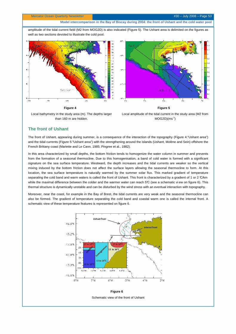
Greetings all,

This month’s newsletter is dedicated to regional and coastal oceanography. We review in this issue the impressive work

recently done towards regional to coastal modelling with nesting and open boundary procedures as well as imbrications of

models of increasing resolution and complexity. Moreover, regional and coastal systems have now reached an operational level

and are delivering real time forecast in various areas.

After an introduction by Obaton reminding us of the challenging European and French programs dealing with regional/coastal

oceanography, this issue displays six scientific articles. Chanut et al. are starting with a paper describing the Mercator Ocean

regional system embracing the French Atlantic coast with a 1/36° horizontal resolution. Marsaleix et a l. are then writing about

the North Western Mediterranean Sea system which is currently upgraded in the framework of the ECOOP program. Next paper

by Riflet et al. is dealing with operational ocean forecasting of the Portuguese waters using the Mercator Ocean North Atlantic

high resolution solution at its boundaries. Lecornu et al. are following with an article about the PREVIMER operational MARS

system in the Bay of Biscay. Marchesiello et al. are then describing the effort conducted at IRD in order to provide the

developing countries with tools for operational regional marine forecast. At last, Reffray et al. tell us how the MARS,

SYMPHONIE and NEMO/OPA systems intercompare over the Bay of Biscay during the year 2004.

We wish you a pleasant reading, and we will meet again in October 2008, with a newsletter dedicated to the international

GODAE project, which will hold its final meeting in Nice on November 12-15 2008 (http://www.godae.org/announcement-II.html).

Moreover, let us also remind you that our annual operational oceanography group meeting (Groupe Mission Mercator Coriolis,

GMMC) will take place on October 13 to 15 2008 in Toulouse (MétéoFrance site). We are looking forward to tell you about our

ongoing progress here at Mercator Ocean, and to hear about yours.

http://www.godae.org/announcement-II.html


GIP Mercator Ocean

Contents

A glance at regional and coastal modelling ...................................................................................................... 3

By Dominique Obaton

Towards North East Atlantic Regional modelling at 1/12° and 1/36° at Mercator Ocean ................................. 4

By Jérôme Chanut, Olivier Le Galloudec, Fabien Léger

Regional Operational Oceanography in the North Western Mediterranean Sea ............................................ 13

By Patrick Marsaleix, Claude Estournel, Muriel Lux

Operational Ocean forecasting of the Portuguese waters .............................................................................. 20

By Guillaume Riflet, Manuela Juliano, Luis Fernandes, Paulo Chambel Leitão, Ramiro Neves

PREVIMER: Operational MARS system in the Bay of Biscay ............................................................................ 33

By Fabrice Lecornu, Pascal Lazure, Valérie Garnier, Alain Ménesguen, Marc Sourisseau

Keys to affordable regional marine forecast systems ..................................................................................... 38

By Patrick Marchesiello, Jérôme Lefèvre, Pierrick Penven, Florian Lemarié, Laurent Debreu, Pascal Douillet, Andres Vega,

Patricia Derex, Vincent Echevin, Boris Dewitte

Model intercomparison in the Bay of Biscay during 2004: the front of Ushant and the cold water pool ........ 49

By Guillaume Reffray, Bruno Levier, Sylvain Cailleau, Patrick Marsaleix, Pascal Lazure, Valérie Garnier


A glance at regional and coastal modelling

A glance at regional and coastal modelling By Dominique Obaton

Mercator Ocean, 8/10 rue Hermès, 31520 Ramonville st Agne, France

Five years ago, coastal modelling was divided around France in different labs and institutes. Aims and study areas were all

different although several teams were developing modelling of the Gulf of Biscay, some of them for operational purposes.

In Spain and France, coastal operational projects had already started for several years. Both have the same objectives: to build

and run an operational model of the Spanish and French coasts respectively. They deal with modelling, as well as with

observations, data management and databases. With 3 models, the national Spanish project ESEOO covers completely the

Atlantic down to the Canaries and Mediterranean Spanish coast. The national French project Previmer, in the same way using 2

models, describes the whole French coastal area including the English Channel, the Gulf of Biscay and the Mediterranean Sea

(see article by Lecornu et al, this issue). Several smaller areas are then downscaled from these operational coastal models for

specific applications and various thematic.

Mercator Ocean has decided to develop a high resolution regional system of South Western Europe (see next article by Chanut

et al., this issue) in order to improve its products near the coast where the needs of intermediate users are the highest. This

system is nested within the global Mercator system and is built to contain more physics, as tides and improved river

parameterisation, than the actual Mercator operational system of the North Atlantic and Mediterranean Sea. The latter system

has been so far used to provide initial and open boundary conditions for coastal model in the area. For coastal modelling needs

out of South Western Europe, it is the global Mercator system that provides initial and boundary conditions.

The Navy SHOM, the POC/CNRS lab and Mercator Ocean started an assessment of their modelling results in the Gulf of

Biscay (see article by Reffray et al., this issue). Rapidly, Ifremer joined as well as later the Portuguese IST modelers. In order to

reduce the degree of freedom for the interpretation of the results, a common set of technical and scientific constraints (same

atmospheric fluxes, bathymetry, horizontal resolution, oceanic forcings and river databases) was adopted by each partner. The

idea is to better understand the cause of possible problems or incorrect representation of the reality from one model to the

other.

The IRD modelling team has developed and used a technique of cascade nesting to reach small domain with very high

resolution in areas where local forcing need be as accurate as possible (see article by Marchesiello et al., this issue).

At the European level, the ECOOP project started a bit later, beginning of 2007. It is coordinated by the Danish Meteorological

institute (DMI) and counts 70 partners around Europe. Its objective is to build a pan European system from a modelling and

observation point of view. It gathers the 5 EuroGOOS regions: Baltic, North Western Shelf, South Western shelf, Mediterranean

Sea and Black Sea. The modelling part consists of a system of system starting from the global Mersea system used to nest the

5 regional EuroGOOS domains, then each regional system provides initial and boundary conditions to 3 coastal models. The

deal is to have, beginning of 2009, this complete embedded system running in real time for a 6 month period and providing data

to a common server database to be viewed and uploaded.

These 5 EuroGOOS regions, plus the Arctic one, are those considered in the MyOcean project. The 6 modelling regional

systems as well as the global system will form the modelling production unit of the European marine core service. Core here

means that products will be hydrodynamic and biological outputs of the systems without any added value and without being

tuned to any specific application. Diffusion of products is planned to be very open to users. We talk about a bulk service.

Applied projects involving coastal modelling people and end users are using this generic service and then create value added

products for coastal applications as beach salubrity, water retreatment, harbour pollution, shellfish farming among others. Links

between these downstream services and the core ones are clear. Needs as well as requests are increasing.

Things have evolved very fast; lots of good and interesting works have been done these past years.


Towards North East Atlantic Regional modelling at 1 /12° and 1/36° at Mercator Ocean

Towards North East Atlantic Regional modelling at 1 /12° and 1/36° at Mercator Ocean By Jérôme Chanut, Olivier Le Galloudec, Fabien Léger

Mercator Ocean, 8/10 rue Hermès, 31520 Ramonville st Agne, France

Introduction

In the recent years, lots of efforts have been invested in the development of the NEMO ocean model

(http://www.lodyc.jussieu.fr/NEMO/) to make it suitable for shelf seas applications. This was mainly achieved thanks to the

MERSEA project and comes from the need expressed by some operational centers to have a single and flexible model to

operate global, basin scale and regional configurations. In a more general perspective, it seems that most of the historically

large scale “climate oriented” models tend now to follow that strategy, progressively filling the gap with coastal models in terms

of numerics. The comparison between NEMO and other coastal ocean models over the Bay of Biscay presented in this issue by

Reffray et al. gives us confidence that NEMO has now sufficient skills to resolve important coastal processes.

As part of the “Façade” project, Mercator Ocean planned to develop a regional forecasting system over the North East Atlantic,

taking advantage of the recent developments in NEMO. Obviously, the goal of this project is to improve the currently global

eddy permitting and eddy resolving Atlantic systems results, refining initial and boundary conditions for the growing number of

coastal users over this area. This note describes the progress made so far in the development of this model. We essentially

focus on the implementation of the tidal forcing currently missing in the large scale and global forecasting systems. With the

recent work of Siddorn et al. (2008), this is indeed one of the first study on tidal modeling with NEMO.

The first part describes the model configuration while the second examines the accuracy of the tidal surface elevation as

simulated by the model with constant density and no atmospheric forcing. Sensitivity to open boundary conditions and tidal

potential are presented. In the third part, impact of tides on the vertical mixing of temperature in a realistic configuration is briefly

commented.

a)

b)

Figure 1

a) FES2004 M2 amplitude in meters (coloured contours, interval=0.25 m) and phase in degrees (white contours, interval=20°).

b) Same as a) but in the 1/36° regional model.

http://www.lodyc.jussieu.fr/NEMO/



Model description

The model code, NEMO v2.3, solves the 3-dimensional Navier Stokes equations in geopotential coordinates under the

hydrostatic and Boussinesq approximations. It is very similar to the one used in the operational systems currently operated by

Mercator Ocean, but there are important differences especially for the treatment of the free surface that need to be mentioned:

• In order to allow fast external gravity waves, the “filtered” free surface (Roullet and Madec, 2000) is replaced by the

time-splitting scheme of Griffies and Pacanowski (2001): The barotropic part of the dynamical equations is integrated

explicitly with a short time step (3 to 9 seconds, depending on the horizontal resolution) while depth varying prognostic

variables (baroclinic velocities and tracers) that evolve more slowly are solved with a larger time step (50 times larger).

Keeping the filtered free surface would induce unrealistic damping of tidal waves as demonstrated by Levier et al

(2007).

• The amplitude of tidal waves becoming large in coastal regions compared to the local depth, the linear free surface

formulation is replaced by the non-linear free surface one recently implemented by Levier et al. (2007). Following the

approach of Stacey et al. (1995), the vertical coordinate z* is rescaled at each model time step according to:

),,(),(

),,(),(*

tyxyxH

tyxzyxHz

ηη

++=

(1)

where z is the “original” height coordinate, η(x,y,t) the sea surface height and H(x,y) the total ocean depth at rest. This

coordinate, commonly used in coastal models but complemented with a terrain following vertical discretization, has

important consequences on the generation of shallow water - higher order - harmonics, residual transports and possibly

on the tidally induced vertical mixing.

Obviously, tidal processes are very sensitive to the time splitting scheme and the non-linear free surface formulation, so that

tests conducted here also provide a stringent validation benchmark for these recently implemented options.

As shown in Figure 1, the model domain spans the whole North East Atlantic, North Sea and part of the Western Mediterranean

Sea. It has been designed essentially to cover most of the coastlines of the IBIROOS (Iberian Biscay Ireland Regional

Operational Oceanographic System) members (Spain, Portugal, Ireland and France). Five open boundary segments connect

the domain with the North Atlantic and Arctic oceans, and the Mediterranean and Baltic Seas. The vertical grid has the same 50

geopotential levels as in the global model with a partial cells representation of the topography (Pacanowski and Gnanadesikan,

1998). The horizontal grid is extracted from the global ORCA bipolar grid also used in global prototypes. This makes open

boundary and initialization data management easier, and allows important conservation properties at the open edges of the

domain. For computational comfort, two sets of horizontal grids are used: a moderate resolution grid of 1/12° (6 km) is used to

perform most of the sensitivity tests, the target resolution being 1/36° (2 km). Bathymetries are deri ved respectively for the

moderate resolution and high resolution grid from ETOPO 2 and GEBCO datasets (since ETOPO 2 is derived from GEBCO for

depths lower than 200m, these are quasi the same on the continental shelf).

Modelling barotropic tides with NEMO

In order to quantify the ability of the model to represent tidal waves propagation, it has been run in a “pseudo barotropic” mode:

Density is held constant, atmospheric forcing is not considered, but the full vertical discretization and turbulence mixing (a 1.5

TKE closure, Gaspar et al., 1990) are taken into account. It is beyond the scope of this note to give an exhaustive description of

the numerous experiments performed. Only selected experiments examining the sensitivity to open boundary schemes/data,

horizontal resolution, tide potential are presented here. These are described below and listed in Table 1.



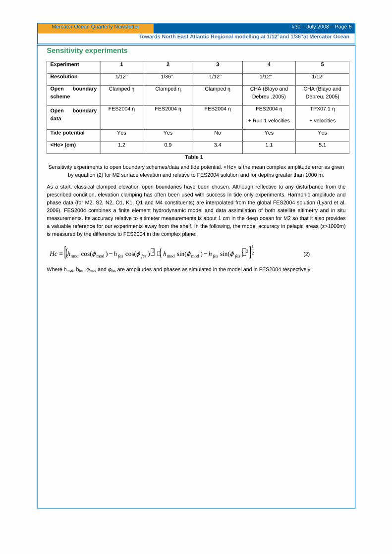
Sensitivity experiments

Experiment 1 2 3 4 5

Resolution 1/12° 1/36° 1/12° 1/12° 1/12°

Open boundary scheme

Clamped η Clamped η Clamped η CHA (Blayo and

Debreu ,2005)

CHA (Blayo and

Debreu, 2005)

Open boundary

data

FES2004 η FES2004 η FES2004 η FES2004 η

+ Run 1 velocities

TPX07.1 η

+ velocities

Tide potential Yes Yes No Yes Yes

<Hc> (cm) 1.2 0.9 3.4 1.1 5.1

Table 1

Sensitivity experiments to open boundary schemes/data and tide potential. <Hc> is the mean complex amplitude error as given

by equation (2) for M2 surface elevation and relative to FES2004 solution and for depths greater than 1000 m.

As a start, classical clamped elevation open boundaries have been chosen. Although reflective to any disturbance from the

prescribed condition, elevation clamping has often been used with success in tide only experiments. Harmonic amplitude and

phase data (for M2, S2, N2, O1, K1, Q1 and M4 constituents) are interpolated from the global FES2004 solution (Lyard et al.

2006). FES2004 combines a finite element hydrodynamic model and data assimilation of both satellite altimetry and in situ

measurements. Its accuracy relative to altimeter measurements is about 1 cm in the deep ocean for M2 so that it also provides

a valuable reference for our experiments away from the shelf. In the following, the model accuracy in pelagic areas (z>1000m)

is measured by the difference to FES2004 in the complex plane:

( ) ( )[ ]2

12

modmod2

modmod )sin()sin()cos()cos( fesfesfesfes hhhhHc ϕϕϕϕ −+−= (2)

Where hmod, hfes, φmod and φfes are amplitudes and phases as simulated in the model and in FES2004 respectively.



a) 1/36° Expt 2 b) 1/12° Expt 1

c) 1/12° Expt 5 d) 1/12° Expt 3

Figure 2

Maps of complex amplitude error Hc (cm) relative to FES2004 for M2 elevation.

Figure 1b shows M2 amplitude and phase maps deduced from a harmonic analysis performed over a 30 days long integration

of the 1/36° model (expt. 2). In the Atlantic Ocean , the solution reflects a Kelvin Wave propagation from the south to the north

with increasing amplitudes towards the shelf which compares well with the FES2004 solution shown in Figure 1a. The pattern in

the North Sea and the English Channel is more complicated with several amphidromic points, which are all well captured by the



model except the degenerate one South of Norway that is shifted on the Western coast of Denmark1. Maximum amplitudes in

the Bristol Channel and the Mont Saint Michel Bay (4.5m) are slightly overestimated but the overall picture appears satisfactory.

The map of complex difference between the model result and FES2004 in Figure 2a shows that discrepancies are essentially

located in coastal regions, notably in the North Sea. This error map is in fact very similar to the standard deviation induced by

changes in bottom friction. In the deep ocean, the average error (0.9 cm) is almost negligible, suggesting that the model solution

adjusts successfully to the imposed open boundary conditions. Pleasingly, increasing the resolution slightly improves the

solution (compare Figure 2a and Figure 2b), decreasing the error in pelagic areas by 10 %. Changes due to resolution are more

significant in coastal areas, particularly in the English Channel and the Irish Sea where the complex coastline is better

represented with a 2 km grid. The same reason probably explains the bias reduction in the Alboran Sea, the Gibraltar Strait

being more realistic in the 1/36° experiment. Final ly, even if the model solution is essentially driven by the boundary conditions,

omitting the tidal potential in dynamical equations (expt. 4) clearly degrades the solution (Figure 2d). Similarly as in the

numerical study of Pairaud (2005), tidal potential reduces M2 amplitude in the Bay of Biscay by about 10 cm.

Another popular open boundary scheme for tidal applications is the Flather (1976) condition very close to the characteristic

method proposed by Blayo and Debreu (2005) used in this study (hereafter CHA). As discussed by Carter and Merrifield (2007),

Flather’s scheme should be preferred in tidal applications because it is less sensitive to open boundary values, allowing both the

computed transport and elevations to adjust to the prescribed data. It therefore requires velocity data, provided here by the

inverse model solution TPXO 7.1 of Egbert and Erofeeva (2002). TPX0 elevation data is very close to the FES2004 solution

(within 1 cm in the deep ocean), so that almost the same results are obtained when using it in clamped elevation experiment.

The accuracy of the velocity data is nevertheless questionable since TPX0 is only constrained by satellite observations. As

shown in Figure 2c, the M2 complex error when using CHA with TPX0 7.1 elevation and transport data (expt. 5) considerably

increases in the western part of the domain with an average error of 5.1 cm relative to FES2004. Amplitude and phase (not

shown) have typical errors of 5 cm and 6° near the western open boundary. Note that a similar issue arises for other semi-

diurnal components, while diurnal harmonics tend to be better represented than in clamped elevation runs. To test the sensitivity

to velocity data, an experiment with CHA open boundary scheme and velocities extracted from the clamped elevation

experiment has been performed (expt. 4). This is reminiscent of the iterative procedure proposed by Flather (1987) to obtain

open boundary velocity data from tidal elevation data only. In that case, the average error is very close to the clamped elevation

run, so that the procedure does not need to be iterated. In contrast, the same experiment, but initialized from TPXO velocities,

needs about 10 iterations to converge. This reveals the difficult adjustment of the model velocities at the open boundaries. Since

the topography on the western open boundary is particularly complicated, this issue could be induced by bathymetry mismatch

between the global TPXO model and the regional one.

Tidal

wave

Period

[hours]

nobs Obs Mean

amplitude

[cm]

Rms amp [cm] /

phase [°]

FES2004

Rms amp [cm] /

phase [°]

TPXO7.1

Rms amp [cm] /

phase [°] NEATL12

(Expt. 2)

Rms amp [cm] /

phase [°] NEATL36

(Expt. 1)

M2 12.44 134 124.6 4.0 / 5.6 7.6 / 4.3 6.5 / 4.9 5.9 / 4.3

S2 12.00 99 40.5 2.4 / 6.9 1.9 / 3.9 2.3 / 4.0 1.8 / 3.9

N2 12.65 96 23.4 1.2 / 6.2 1.1 / 3.8 1.5 / 4.2 1.4 / 3.9

O1 25.81 98 6.6 0.5 / 5.9 0.6 / 7.2 0.5 / 5.2 0.5 / 5.0

K1 23.93 98 7.3 0.8 / 7.6 0.7 / 9.8 1.3 / 8.3 1.3 / 8.5

Q1 26.86 69 2.2 0.3 / 13.3 0.3 / 10.8 0.4 / 11.2 0.4 / 10.9

Table 2

Rms errors between observed and computed tidal elevation amplitude and phase (measurement locations are shown in Figure

(3). NEATL12-T46 and NEATL12-T46 are tide only runs at respectively 1/12° and 1/36° resolution.

1 Complementary experiments have shown that the position of this amphidromic point is very sensitive to the minimum ocean

depth in the model (which must be greater than the maximum elevation since NEMO does not deal with wetting and drying

processes yet). Reducing it from 10 meters to 3 meters in the North Sea solves the problem.



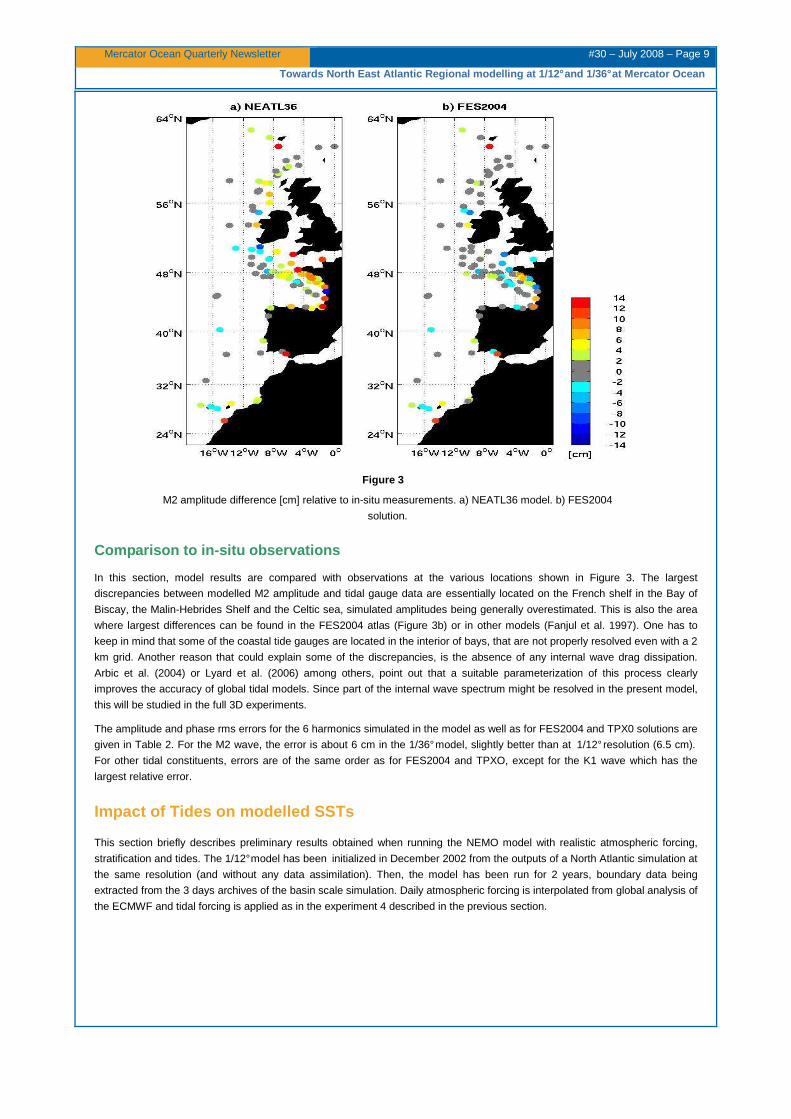
Figure 3

M2 amplitude difference [cm] relative to in-situ measurements. a) NEATL36 model. b) FES2004

solution.

Comparison to in-situ observations

In this section, model results are compared with observations at the various locations shown in Figure 3. The largest

discrepancies between modelled M2 amplitude and tidal gauge data are essentially located on the French shelf in the Bay of

Biscay, the Malin-Hebrides Shelf and the Celtic sea, simulated amplitudes being generally overestimated. This is also the area

where largest differences can be found in the FES2004 atlas (Figure 3b) or in other models (Fanjul et al. 1997). One has to

keep in mind that some of the coastal tide gauges are located in the interior of bays, that are not properly resolved even with a 2

km grid. Another reason that could explain some of the discrepancies, is the absence of any internal wave drag dissipation.

Arbic et al. (2004) or Lyard et al. (2006) among others, point out that a suitable parameterization of this process clearly

improves the accuracy of global tidal models. Since part of the internal wave spectrum might be resolved in the present model,

this will be studied in the full 3D experiments.

The amplitude and phase rms errors for the 6 harmonics simulated in the model as well as for FES2004 and TPX0 solutions are

given in Table 2. For the M2 wave, the error is about 6 cm in the 1/36° model, slightly better than at 1/12° resolution (6.5 cm).

For other tidal constituents, errors are of the same order as for FES2004 and TPXO, except for the K1 wave which has the

largest relative error.

Impact of Tides on modelled SSTs

This section briefly describes preliminary results obtained when running the NEMO model with realistic atmospheric forcing,

stratification and tides. The 1/12° model has been initialized in December 2002 from the outputs of a North Atlantic simulation at

the same resolution (and without any data assimilation). Then, the model has been run for 2 years, boundary data being

extracted from the 3 days archives of the basin scale simulation. Daily atmospheric forcing is interpolated from global analysis of

the ECMWF and tidal forcing is applied as in the experiment 4 described in the previous section.



Figure 4

Observed (black line) and simulated Sea Surface temperature [°C] in Cherbourg (sea location (Black Sta r) on Figure 5a) with

explicit tidal forcing (red line) and without explicit tidal forcing (green line).

a) b)

c) d)

Figure 5

a) July 2004 MODIS SST. b) Corresponding modelled SST without explicit tidal forcing. c) Same as b) but with explicit tidal

forcing. d) Model monthly statistics over the North Sea region relative to satellite derived SST. Continuous lines correspond to

the 1/12° simulation with tidal forcing while dashe d lines to the standard simulation without tidal forcing. Blue stands for the

correlation, Red for the mean deviation and Black for the Root Mean Square deviation.



In order to evaluate the model ability to reproduce the Sea Surface Temperature (SST) structure, results were compared to the

4km MODIS satellite data over the year 2004. MODIS SST in July 2004 is shown in Figure 5a over the North Sea and can be

compared to the model result with or without tidal forcing, respectively in Figure 5c and Figure 5b for the same time period. The

occurrence of thermal fronts in the English Channel, in the Western Irish Sea and south of the Shetlands Islands is particularly

evident when tidal forcing is active and well reproduced by the model. These fronts are however not as sharp as in

observations, probably because of the moderate resolution used here. It is expected that the 1/36° gri d, with less diffusion and

ad hoc advection schemes would improve the results. All in all, the statistical results summarized in Figure 5d, show that adding

tidal forcing significantly decreases the RMS error, at least during the summer period. This is supported by the systematic

comparison to various in situ measurements, such as the one in Cherbourg shown in Figure 4.

Conclusions

Progress in the development of a regional forecasting model over the North East Atlantic has been presented. We essentially

focused on the implementation of tidal forcing and briefly described its impact on the simulated summertime SSTs. We have

shown that the model successfully simulates tidal waves, errors on sea surface elevations being comparable to other regional

tidal models in this region such as the one of Fanjul et al. (1997). The comparison to satellite derived SST reveals that the

additional mixing induced by the tides improves the results, decreasing the model tendency to overestimate SSTs in the North

Sea.

On a numerical point of view, this study demonstrates that the recently implemented splitting algorithm based on the MOM

code (Griffies and Pacanowski 2001) for climate modeling purposes is also efficient for tidal modeling. The same conclusion

was drawn by Schiller and Fiedler (2007) with the MOM code. Although this has not been detailed in this note, shallow water

constituents simulated in the model such as the M4 tidal wave compare well with observations and other model results. This

gives us confidence in the way the non linear free surface is implemented (Levier et al. 2007). Indeed, as shown by Fanjul et al.

(1997), non-linearity in the continuity equation introduced by the rescaled height coordinate (1) explains roughly half of the M4

wave amplitude in the Bay of Biscay.

Future work will now essentially concentrate on the 1/36° version of the model. Tide-only experiments shown here, already

suggest a slight improvement compared to the 1/12° version. Moving to the full 3d version has now started, but still represents a

computational challenge: roughly half of the 1/12° global model CPU time is required to run the 1/36° North East Atlantic model.

Acknowledgments

We would like to thank Florent Lyard for helpful discussions and sharing tide gauges harmonic data. Many thanks also to

colleagues of the regional modeling team in Mercator for their help in setting up the model and to Laurence Crosnier for her

suggestions. The MODIS SST data were obtained from the Physical Oceanography Distributed Active Archive Center

(PO.DAAC) at the NASA Jet Propulsion Laboratory, CA (http://podaac.jpl.nasa.gov).

References

Arbic, B. K., S. T. Garner, R. W. Hallberg and H. L. Simmons, 2004: The accuracy of surface elevations in forward global

barotropic and baroclinic tide models. Deep-Sea Research II, 51, 3069-3101.

Blayo, E. and L. Debreu, 2005: Revisiting open boundary conditions from the point of view of characteristic variables. Ocean

Modelling, 9, 231-252.

Carter, G.S. and S.Y. Merrifield, 2007: Open boundary conditions for regional tidal simulations. Ocean Modelling, 18, 194-209.

Egbert, G.D., Erofeeva, S.Y., 2002: Efficient inverse modelling of barotropic ocean tides. J. Atm. Ocean. Tech., 19(2), 183-204.

Fanjul, E.A., B.P. Gomez and I.R. Sanchez-Arevalo, 1997: A description of the tides in the Eastern North Atlantic. Prog.

Oceanogr., 40, 217-244.

Flather, R. A., 1976: A tidal model of the north-west European continental shelf. Memoires de la Societe Royale des Sciences

de Liege, 6(10), 141-164.

Flather, R. A., 1987: A tidal model of the north-east Pacific. Atmospher-Ocean,, 25, 22-45.

Gaspar, P., Y. Gregoris and J. M. Lefevre, 1990: A simple eddy-kinetic-energy model for simulations of the ocean vertical

mixing: tests at station Papa and Long-Term Upper Ocean Study site. J. Geophys. Res., 95, 16, 179-16,193.

Griffies, S. M. and R. C. Pacanowski, 2001: Tracer conservation with explicit free surface method for z-Coordinate ocean

models. Monthly Weather Review, 129, 1081-1098.



Levier, B., A. M. Tréguier, G. Madec and V. Garnier, 2007: Free surface and variable volume in the NEMO code. MERSEA IP

report WP09-CNRS-STR03-1A, 47pp.

Lyard, L., F. Lefevre, T. Letellier and O. Francis, 2006: Modelling the global ocean tides: modern insights from FES2004. Ocean

Dyn., 56, 394-415.

Pacanowski, R. C. and A. Gnanadesikan, 1998: Transient response in a Z-Level Ocean Model that Resolves Topography with

Partial Cells. Monthly Weather Review, 126, 3248-3270.

Pairaud, I., 2005: Modélisation et analyse de la marée interne dans le Golfe de Gascogne. Phd Thesis, Université Toulouse III -

Paul Sabatier.

Roullet, G., and G. Madec, 2000: Salt conservation, free surface and varying volume: a new formulation for Ocean GCMs. J.

Geophys. Res.,105 , 23927-23942.

Schiller, A. and R. Fiedler, 2007: Explicit tidal forcing in an ocean general circulation model. Geophys. Res. Letters, 34, LO3611,

doi:10.1029/2006GL028363.

Siddorn, J., J. Holt, R. Maydon, E. O’Dea, D. Storkey and G. Riley, 2008: Mersea Developments at the Met Office. Mercator

Quarterly newsletter, April 2008.

Stacey, M. W., Pond, S. Nowak, Z.P., 1995: A numerical model of the circulation in knight inlet, British Columbia, Canada. J.

Phys. Oceanogr., 25, 1037-1062.


Regional Operational Oceanography in the North West ern Mediterranean Sea

Regional Operational Oceanography in the North West ern Mediterranean Sea By Patrick Marsaleix 1, Claude Estournel 1, Muriel Lux 2

1 POC/Laboratoire d’Aérologie, Université de Toulouse et CNRS, 14 Avenue Edouard Belin, 31400 Toulouse, France 2 Noveltis, Avenue de l’Europe, 31520 Ramonville Saint Agne, France

Introduction

Operational oceanography has been developed over the last decade in conjunction with the near-real time availability of satellite

altimetry and in-situ observations which allow constraining ocean models. Operational oceanography first concerned three

domains being storm surges, sea state and 3D basin-scale circulation forecasting. The ocean circulation forecasting gave rise to

several systems which release analyses and forecasts at time scales of the order of one week and at spatial scales of 5 to 10

kilometers. The availability of these basin scale (henceforth OGCM) products has permitted to develop regional or coastal

systems with the aim of performing forecasts in the coastal zone. These systems must be adapted to the specificities of the

coastal zones with a complex topography, the potential presence of strong tidal currents, the vicinity of the continent which

influences the atmospheric flow at small and meso scales and the freshwater riverine inputs. Taking into account these

constraints, the MFS (Mediterranean Forecasting System, Pinardi et al., 2007) program proposed a strategy of downscaling

from the basin scale to the coastal scale based on specific methods and forcing. These operational systems have been

implemented in several regions of the Mediterranean Sea since 2004. In this framework, the POC group and the NOVELTIS

Company have set up a prototype of the North Western Mediterranean Sea (Estournel et al., 2007). This system is currently

upgraded in the framework of the pan-European program ECOOP (European Coastal Sea – Operational Observing and

Forecasting System). In this letter, we display the latter system and its evolutions.

Strategy for coastal operational forecasting

The first constraint of the coastal circulation is the presence of steep bathymetric slopes which concentrate currents and across

which exchanges between continental shelf and deep sea operate. It is recognized that the use of sigma vertical coordinate

(more or less sophisticated) is necessary to correctly represent this region. An extreme case is the example of gravity currents

which flow down the bathymetric slope which are badly represented by staircases vertical discretization. Besides, the coastal

zone is characterized by a strong high frequency dynamic (e.g. tide) leading to the generalized use of free surface models.

Finally, the simulated geographic domains generally have extended open boundaries where external fields obtained from the

OGCM model are required to force the inner solution and where waves should be allowed to radiate out or water masses to

leave the modelling domain under outgoing conditions, without any spurious reflections.

The North Western Mediterranean (NWMED) forecasting system is based on the hydrostatic Boussinesq ocean model

Symphonie which uses energy-conserving numerical schemes (Marsaleix et al, 2008). This free surface model uses a time

splitting technique to compute separately baroclinic and barotropic processes. Open boundaries are based on stability criteria,

on mass and energy conservation arguments, and on the ability to enforce external information (Marsaleix et al., 2006). Optimal

extrapolation and mass balance enforcement are carried out before larger scale fields are used to initialize and force the high

resolution coastal model along its open boundaries. This is obtained thanks to the Variational Initialization and Forcing Platform

VIFOP (Auclair et al., 2006). The first objective of this variational optimization strategy is to ensure that the forcing fields satisfy

the fundamental mass balance. The second objective is to reduce the generation of surface gravity waves due to a local mass

imbalance. The VIFOP platform is used by several partners of MFS to downscale the Mediterranean Sea circulation in their

coastal regions (e.g. Zodiatis et al., 2006).

Symphonie has been implemented on the northwestern Mediterranean Sea area (figure 1) with 40 vertical generalised sigma

levels and 1/32°x1/32° horizontal meshes using the daily 1/16° analyses produced by MFS (Dobricic et a l., 2007). Recent

applications of Symphonie on this particular region are given by Ulses et al. (2008), and Herrmann et al. (2008).



Figure 1

Bathymetry (m) of the numerical domain

A major stake of MFS was that the meteorological forcing had to be adapted to coastal regions. The objective is to get accurate

representation of currents, vertical velocities associated with Ekman pumping and high frequency dynamics such as sea level

variations and diurnal cycle of surface layer. The northern coast of the Mediterranean Sea (e.g. the Gulf of Lion) is probably the

area where the need for high resolution atmospheric forcing is the most crucial due to the prevailing wind blowing from land and

then strongly influenced by orography. In the framework of MFS, we used hourly analyses and forecasts from the ALADIN

model with a resolution of 0.1° (Brožková et al., 2 006).

Concerning operational protocol, two strategies can be implemented, each one having assets and drawbacks. In the slave

mode, each forecast is initialized from the OGCM while in the active mode, the coastal model is initialized only once and then

only constrained by the OGCM at its lateral boundaries. The asset of the slave mode is that the coastal model benefits from

data assimilation at each initialization of the OGCM while in the active mode, this information is transmitted only through the

boundary conditions. The slave mode has two drawbacks: first the coastal model needs a spin-up time in order to adapt the

initial state to its better resolved topography and physics (numerical spin-up) and also to develop small scale structures allowed

by its horizontal resolution (physical spin-up). Second, re-initialization does not allow keeping some locally-generated features

such as river plumes. A stake of coastal operational models is to find the procedure best solving those different constraints.

The NWMED operational model has been run in slave mode. In order to reduce the drawbacks of this mode, each simulation

begins with a hindcast before each forecast. The objective is to allow the development of small scale features (Estournel et al.,

2007). The length of the hindcast has to be short for logistic reasons (computational cost) and to avoid a loss of predictability

linked to the errors growth. We found that a compromise of a one-week hindcast allows the development of scales not solved by

the OGCM. The weekly operational procedure begins as soon as meteorological and OGCM analyses and forecasts are

released with a one-week hindcast followed by a five-day forecast. In the ECOOP project, we study improvements of the

forecasting procedure on two important points. First the active mode should be implemented with the aim of continuously

following the locally-generated features. It is however not conceivable to use this mode without taking care of slowly diverging

solution from the OGCM forced at the open boundaries (for example due to heat or water budget difference between the two

models). A study is on-going in order to drive the large scale features of the coastal model toward the OGCM while leaving free

the development of small scales. The second point concerns data assimilation. Assimilation in coastal zone presents difficulties

linked to the anisotropy of circulation strongly constrained by bathymetry in these regions. The correction of altimetric data in

coastal zones is currently a major axis of research but the physical content of these data is a complex mixing of processes and

time scales making their assimilation not straightforward. At first, we propose to assimilate the weekly gridded absolute dynamic

topography fields at the regional scale to better constrain the slope currents which interact with the coastal zone.

These products are provided by AVISO (http://www.aviso.oceanobs.com/en/home/index.html) on a 1/8°X1/8° regular grid. The

AVISO data field gives a synoptic view of the sea surface height (hereafter SSH) of the Mediterranean Sea with enough

resolution to access to the low frequency thermohaline geostrophic circulation. On the one hand, it can be used to help the

model improving its representation of the regional circulation of the North Western Mediterranean Sea, notably the synoptic

cyclonic gyre generally identified as the Liguro-Provençal-Catalan current (hereafter LPC). On the other hand, owing to the lack

of resolution and some practical limitations (near-shore altimetric signal is unexploitable), this type of data does not give access



to high frequency processes, small scale features, nor to the continental shelf dynamics. Practically, this excludes wind driven

patterns, slope current meanders, upwellings, rivers plumes.

Here, we present a preliminary step that aims at estimating the feasibility of the method. In order to do this, the AVISO dynamic

topography maps have been replaced by the outputs of the OGCM which is the Mediterranean basin model from the MFS

project. The interest of substituting observed SSH by modelled SSH fields is the possibility to use the OGCM model variables,

i.e. temperature, salinity and currents (hereafter T, S, u and v) as validation variables. If the assimilation of the SSH lead to a

general reduction of the gap (not only for SSH but also for T, S, u and v) between the OGCM fields and the NWMED model

fields, the assimilation method is pertinent.

Description of the assimilation method

The forecast run is preceded by a one week hindcast simulation forced by the meteorological and OGCM analysis. The hindcast

simulation is computed twice. The first run (hindcast A Priori), performed without data assimilation, is used to

compute prioriaη , a week average of the SSH field. The latter is compared to obsη a corresponding reference SSH. As

previously mentioned, the reference field is here provided by a week average of the OGCM solution for the sake of the

validation purpose, but will be given by the AVISO fields during the operational phase of the ECOOP project. In order to make

the NWMED model outputs consistent with the coarser grid of the reference field, length scales shorter than °8/1 are removed

from prioriaη . The aim of the assimilation procedure is to reduce the magnitude of the SSH anomaly obsη - prioriaη thanks

to the second hindcast run (hindcast Update) performed over the same period of time and using the same external forcing,

except that some new adjustments are brought to the thermohaline model structure. The principle of the method, basically that

of Cooper and Haines (1996) (hereafter CH96), is based on the fact that the low frequency response of the surface pressure to

a density field perturbation mainly intends at keeping the bottom hydrostatic pressure unchanged. Let the aforementioned

density anomaly be of the form: Rδργρ =∆ , where Rδρ is an priori density vertical profile and γ a control parameter of the

bottom pressure perturbation. The bottom pressure perturbation induced by density effects is given by:

∫−=0

'h Rb dzgp δργ (1)

The hypothesis that the total bottom pressure should remain unchanged permits to estimate ηρ ∆0g , the surface pressure

response, according to:

0'0 =+∆ bpg ηρ (2)

From (1) and (2) it is possible to deduce a value for γ such that a density perturbation, Rδργρ =∆ , added to the model

density field, will drive the SSH of the hindcast Update toward the reference field, namely:

( )∫−

−−= 0

0

h R

prioriaobs

dzδρ

ηηργ (3)

As density is not a model variable, the density perturbation is built from perturbations of the T and S fields through the equation

of state of the model. Besides, we noticed that the method appears to work better if, as in CH96, a consistent perturbation of the

velocity field is also applied. Considering the time and spatial scales of the problem, the latter is simply deduced from the

hypothesis of geostrophic equilibrium with the pressure perturbation. As in CH96, the concept of observations and model errors

has been neglected so that the hindcast Update uses the full SSH anomaly obsη - prioriaη , except in shallow areas where a

reduced SSH anomaly is considered. This exception intends to take into account the fact that the “no bottom pressure change”

assumption sustaining Eq (2) becomes questionable on the continental shelf.

• Note that some noticeable modifications have been brought to the genuine CH96 method. First of all, Rδρ is not obtained

by assuming a uniform vertical displacement of the water column. It is actually deduced from the hindcast A Priori from

which a one-week average of the T & S anomaly field is computed and then converted into a density anomaly thanks to the

model linear equation of state, namely:

prioriaobsR ρρδρ −= (4)



If the hypothesis made by the assimilation scheme are valid, we can expect γ to be close to one, in other words we can expect

that the SSH and the density anomaly fields will both be reduced by the hindcast Update. If not, (for instance CH96 underline

that the method does not work if the flow is strongly barotropic), density errors are likely to grow, and possibly also SSH errors.

This particular way of computing Rδρ is actually motivated by the present validation purpose but during the operational phase

this could be replaced by a statistical approach, for instance a local EOF analysis of the NWMED solution. We noticed that a

possible shortcoming of (4) is to introduce a discontinuity at the base of the surface mixed layer depth, which can be

significantly different in the NWMED model and the OGCM. It was then decided in a first approach to cancel Rδρ within the

first 100 meters under the sea surface.

• Another difference with CH96 is that density and geostrophic current adjustments are not abruptly applied to the initial state

of the hindcast Update. Following a time integrated approach, perturbation fields are progressively added along the

simulation, through extra forcing terms included in the tracer and momentum model equations. The interest is to ensure the

continuity of the hincast runs and to remove the spin-up effect of classic sequential re-initialisation methods

• Figure 2 presents the operational protocol. Every week, the hindcast A priori is computed first. Then the hindcast with

assimilation (hindcast Update) is computed. The hindcast Update simulations are the elements of a continuous single

simulation. At the end of each hindcast Update, the simulation is extended by the forecast run.

Figure 2

Operational protocol. Gray arrows represent the hindcast A Priori. Black arrows represent the hindcast Update. Red arrows

represent the forecast run.

Preliminary results

The method is tested with a set of three 100 days long simulations of the NWMED starting on December 11 2004. The first

simulation (S1) is performed without assimilation. A second simulation (S2) is performed with the assimilation of the week

average of the OGCM SSH. In both cases, a global estimate of the (SSH, T, S, u, v) errors is computed according to:

( )∫ −= − dSS prioriaobs21 ηηεη (5)

where the integral symbol represents a surface integral over S, the numerical domain area, and:

( )∫ −= − dVTTV prioriaobsT21ε (6)

( )∫ −= − dVSSV prioriaobsS21ε (7)

( ) ( )∫

−+−= − dV

vvuuV prioriaobsprioriaobs

K 2

221ε (8)



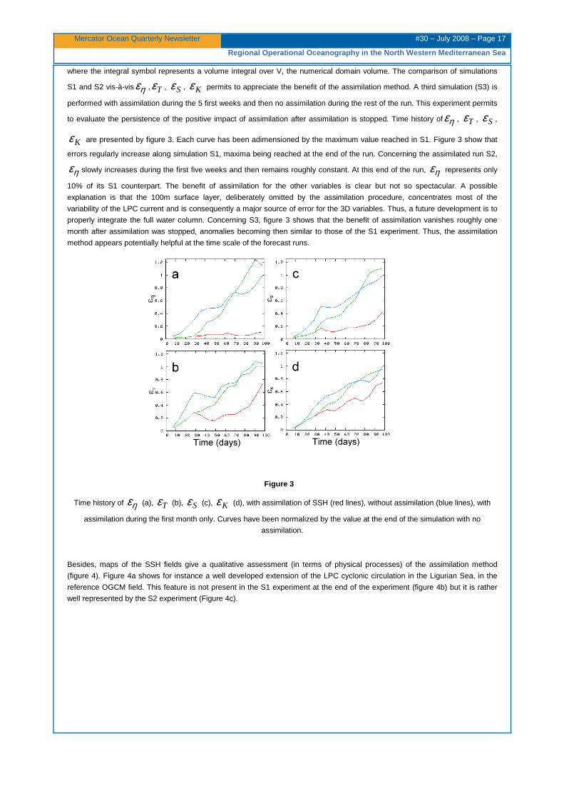
where the integral symbol represents a volume integral over V, the numerical domain volume. The comparison of simulations

S1 and S2 vis-à-vis ηε , Tε , Sε , Kε permits to appreciate the benefit of the assimilation method. A third simulation (S3) is

performed with assimilation during the 5 first weeks and then no assimilation during the rest of the run. This experiment permits

to evaluate the persistence of the positive impact of assimilation after assimilation is stopped. Time history of ηε , Tε , Sε ,

Kε are presented by figure 3. Each curve has been adimensioned by the maximum value reached in S1. Figure 3 show that

errors regularly increase along simulation S1, maxima being reached at the end of the run. Concerning the assimilated run S2,

ηε slowly increases during the first five weeks and then remains roughly constant. At this end of the run, ηε represents only

10% of its S1 counterpart. The benefit of assimilation for the other variables is clear but not so spectacular. A possible

explanation is that the 100m surface layer, deliberately omitted by the assimilation procedure, concentrates most of the

variability of the LPC current and is consequently a major source of error for the 3D variables. Thus, a future development is to

properly integrate the full water column. Concerning S3, figure 3 shows that the benefit of assimilation vanishes roughly one

month after assimilation was stopped, anomalies becoming then similar to those of the S1 experiment. Thus, the assimilation

method appears potentially helpful at the time scale of the forecast runs.

Figure 3

Time history of ηε (a), Tε (b), Sε (c), Kε (d), with assimilation of SSH (red lines), without assimilation (blue lines), with

assimilation during the first month only. Curves have been normalized by the value at the end of the simulation with no

assimilation.

Besides, maps of the SSH fields give a qualitative assessment (in terms of physical processes) of the assimilation method

(figure 4). Figure 4a shows for instance a well developed extension of the LPC cyclonic circulation in the Ligurian Sea, in the

reference OGCM field. This feature is not present in the S1 experiment at the end of the experiment (figure 4b) but it is rather

well represented by the S2 experiment (Figure 4c).



Figure 4

Maps of the SSH (m) after 100 days of run. OGCM solution (a), regional run without assimilation or S1 experiment (b), regional

run with assimilation of the SSH or S2 experiment (c).

Perspectives

Several axes of research are followed in order to improve the operational strategy at regional scale. The data assimilation

described in this paper, coupled with a method allowing not diverging from the OGCM large scale features, seems to be an

interesting active mode offering a time-continuous description of the ocean.

On a longer term, improved coastal SSH data fields based on more accurate treatments and combination with coastal tide

gauges should be delivered by the “observation systems work packages” of the ECOOP projet allowing better performances of

the operational system. Another important stake will be the development of assimilation of local observations (T and S profiles).



Acknowledgements

This study was funded by the European MFSTEP Project (EU Contract EVK3-CT-2002-00075), the European INSEA Project

(SST4-CT-2005-012336) and the ECOOP project. The authors thank Cyril Nguyen and the Laboratoire d’Aérologie computer

team, Serge Prieur, Laurent Cabanas, Jérémy Leclercq, Didier Gazen, and Juan Escobar for their support.

References

Auclair F., Estournel C., Marsaleix P., Pairaud I. 2006. On coastal ocean embedded modeling. Geophysical Research Letters,

33, L14602. DOI:10.1029/2006GL026099

Brožková R., Derková M., Belluš M., and Farda A., 2006. Atmospheric forcing by ALADIN/MFSTEP and MFSTEP oriented

tunings. Ocean Sci., 2, 113-121.

Cooper M., Haines K., 1996. Altimetric assimilation with water property conservation. Journal of Geophysical Reasearch, 101,

C1, 1059-1077

Dobricic, S., Pinardi, N., Adani, M., Tonani, M., Fratianni, C., Bonazzi, A., and Fernandez, V.: Daily oceanographic analyses by

Mediterranean Forecasting System at the basin scale, Ocean Sci., 3, 149-157, 2007.

Estournel C., Auclair F., Lux M., Nguyen C., and Marsaleix P., 2007. “Scale oriented” embedded modeling of the North-Western

Mediterranean in the frame of MFSTEP. Ocean Sci. Discuss., 4, 145–187.

Herrmann, M. J., S. Somot, F. Sevault, C. Estournel, and M. Déqué, 2008. Modeling the deep convection in the northwestern

Mediterranean Sea using an eddy-permitting and an eddy resolving model: Case study of winter 1986-1987. Journal of

Geophysical Research, 113, C04011.

Marsaleix P., Auclair F., and Estournel C., 2006, Considerations on Open Boundary Conditions for Regional and Coastal Ocean

Models. Journal of Atmospheric and Oceanic Technology, 23,1604-1613.

Marsaleix P., Auclair F., Floor J. W., Herrmann M. J., Estournel C., Pairaud I., and Ulses C., 2008. Energy conservation issues

in sigma-coordinate free-surface ocean models. Ocean Modelling, 20, 61-89.

Pinardi, N., Coppini, G., Dobricic, S., Fratianni, C., Tonani, M., Oddo, P., Manzella, G. M. R., Tziavos, C., Nittis, K., Larnicol, G.,

Poulain, P.-M., Send, U., Raicich, F., Griffa, A., Crispi, G., De Mey, P., Lascaratos, A., Sofianos, S., Kallos, G., Katsafados, P.,

Pytharoulis, I., Zavatarelli, M., Triantafyllou, G., Zodiatis, G., and Petit De La Villeon, L.: The Mediterranean ocean Forecasting

System, Bull. Am. Meteorol. Soc., submitted, 2007.

Ulses, C., C. Estournel, J. Bonnin, X. Durrieu de Madron, and P. Marsaleix 2008. Impact of storms and dense water cascading

on shelf-slope exchanges in the Gulf of Lion (NW Mediterranean). Journal of Geophysical Research 113, C02010

Zodiatis, G., Lardner, R., Hayes, D. R., Georgiou, G., Sofianos, S., Skliris, N., and Lascaratos, A.: Operational coastal ocean

forecasting in the Eastern Mediterranean: implementation and evaluation, Ocean Sci. Discuss., 3, 397-434, 2006.


Operational Ocean forecasting of the Portuguese wat ers

Operational Ocean forecasting of the Portuguese wat ers By Guillaume Riflet 1, Manuela Juliano 2, Luís Fernandes 1, Paulo Chambel Leitão 3, Ramiro

Neves 1

1Maretec, Instituto Superior Técnico, Departamento de mecânica, Secção Energia e Ambiente, Av. Rovisco Pais 1, 1049-000 Lisbon, Portugal 2Laboratory of Marine Environment and Technology, University of the Azores, Praia da Vitória, Azores, Portugal 3Hidromod, modelação em engenharia, Av. Manuel da Maia nº 36, 3º esq. 1000-201 Lisbon, Portugal

Introduction

The MOHID numerical system developed by Instituto Superior Técnico (IST, Portugal) with the collaboration of Hidromod

(Portugal) aims at simulating the main physical and biogeochemical processes in marine environments (http://www.mohid.com).

This system is highly disseminated in the Atlantic region (Europe and South America). The support forum has presently 1360

registered users. Many of the applications are in coastal waters with a focus on environmental impacts at the local scale. One of

the difficulties of this type of application is the definition of realistic open boundary conditions. The downscaling of solutions like

the one provided by Mercator Ocean appears to be the best way to overcome this problem.

IST and Hidromod have developed a methodology that allows a MOHID user to downscale a low frequency pre-operational

solution and to add tide to the solution (Leitão et al 2005). Tide is one of the main driving mechanisms in coastal applications.

This methodology was first tested in the Portuguese Algarve waters, where realistic atmospheric and tide forcing were used

(Leitão et al 2005). Several works are being performed to downscale other larger scale solutions using the same methodology.

Furthermore, several past, on-going and future projects such as INSEA, ECOOP, EASY and MYOCEAN are benefiting directly

from such methodology in order to develop useful forecasting systems and bulletin services to end-users such as fisheries and

water-quality public institutions.

In particular, the Mercator Ocean North Atlantic high resolution (PSY2V2) solution is being downscaled in the scope of an

operational system for the Portuguese continental coast (Riflet et al 2007) and, for the first time, for the Azores region. The

present paper describes two systems: one for the West Iberia which is already operational, and another one for the Azores area

which is on its way of becoming operational.

Drillet et al (2005) perform, to some extent, an overall assessment of the Mercator solution for western Iberia. However, for the

Azores region, a comparison of the PSY2V2 solution with climatological data (Juliano et al 2007) was required before analyzing

the models results, yielding a very good agreement.

The results presented in this newsletter focus namely on the Mediterranean outflow spreading pathway and the ENACW (East

North Atlantic Current Water) entrainment near the gulf of Cadiz for the continental Portuguese area and in the Azores Current

Front system for the Azores region. Comparison of the model results with in-situ data was performed on both regions.

Methodology

The operational system

For the west Iberia coast, a three-level nested three-dimensional hydrodynamic model was applied and refined near the

Estremadura promontory using MOHID. Another model with the same forcing and nesting techniques was implemented in the

Azores region, for the first time. The results were compared with in situ data. Realistic forcing was used and provided by the

large-scale North-Atlantic Mercator Ocean (Drillet et al 2005) solution and by the atmospheric MM5 model from meteo-IST

(Domingos et al 2005) for the West Iberian coast, and by the MM5 meteorological outputs provided by the operational

forecasting system of the University of the Azores (http://www.climaat.angra.uac.pt/) for the Azores region. Tide is forced using

the FES2004 solution (Lyard et al 2006). The PSY2v2 Mercator Ocean solution consists of a weekly 14 day forecast and 7 day

analysis. Horizontal resolutions of the models used with MOHID vary from 0.06º to 0.02º with a vertical discretization identical to

PSY2v2 of 43 cartesian layers. The meteo-IST solution consists in a 7 day atmospheric forecast. The atmospheric models have

27 km and 9 km of horizontal resolution (coarser and finer grids) for western Iberia region while for the Azores region, the

coarser domain has 18 km, and the finer domain has 6 km of horizontal resolution.

A pre-operational system was mounted at Maretec-IST that pre-processes the forcing solution, runs the hydrodynamical model

and serves every Monday now casts and forecasts, until Thursday, of the general circulation off west Iberia. In Figure 1 the

nested domains for the Western Iberia region are represented. The results are stored in netcdf files and served on an Opendap

(Doty et al 2001) server. The models are scheduled to run the past 7 days in analysis mode and the next 7 days in forecasting



mode. Results of the continental Portuguese domain are hosted on an Opendap server and weekly runs can be inspected at

http://data.mohid.com/data.xml, where Portugal and Estremadura projects are the 3D1 and 3D2 domains (as described in the

next section), for western Iberia.

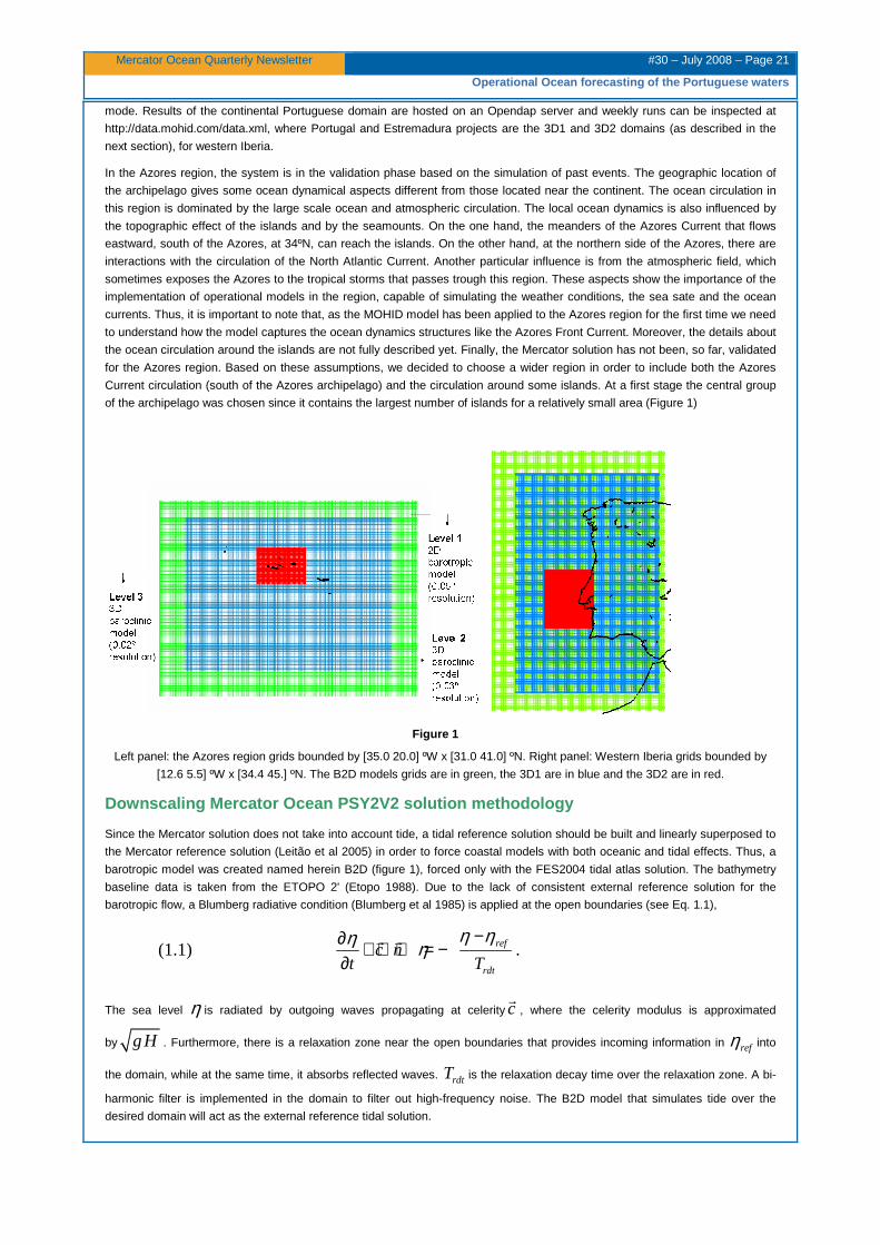
In the Azores region, the system is in the validation phase based on the simulation of past events. The geographic location of

the archipelago gives some ocean dynamical aspects different from those located near the continent. The ocean circulation in

this region is dominated by the large scale ocean and atmospheric circulation. The local ocean dynamics is also influenced by

the topographic effect of the islands and by the seamounts. On the one hand, the meanders of the Azores Current that flows

eastward, south of the Azores, at 34ºN, can reach the islands. On the other hand, at the northern side of the Azores, there are

interactions with the circulation of the North Atlantic Current. Another particular influence is from the atmospheric field, which

sometimes exposes the Azores to the tropical storms that passes trough this region. These aspects show the importance of the

implementation of operational models in the region, capable of simulating the weather conditions, the sea sate and the ocean

currents. Thus, it is important to note that, as the MOHID model has been applied to the Azores region for the first time we need

to understand how the model captures the ocean dynamics structures like the Azores Front Current. Moreover, the details about

the ocean circulation around the islands are not fully described yet. Finally, the Mercator solution has not been, so far, validated

for the Azores region. Based on these assumptions, we decided to choose a wider region in order to include both the Azores

Current circulation (south of the Azores archipelago) and the circulation around some islands. At a first stage the central group

of the archipelago was chosen since it contains the largest number of islands for a relatively small area (Figure 1)

Figure 1

Left panel: the Azores region grids bounded by [35.0 20.0] ºW x [31.0 41.0] ºN. Right panel: Western Iberia grids bounded by

[12.6 5.5] ºW x [34.4 45.] ºN. The B2D models grids are in green, the 3D1 are in blue and the 3D2 are in red.

Downscaling Mercator Ocean PSY2V2 solution methodol ogy

Since the Mercator solution does not take into account tide, a tidal reference solution should be built and linearly superposed to

the Mercator reference solution (Leitão et al 2005) in order to force coastal models with both oceanic and tidal effects. Thus, a

barotropic model was created named herein B2D (figure 1), forced only with the FES2004 tidal atlas solution. The bathymetry

baseline data is taken from the ETOPO 2' (Etopo 1988). Due to the lack of consistent external reference solution for the

barotropic flow, a Blumberg radiative condition (Blumberg et al 1985) is applied at the open boundaries (see Eq. 1.1),

(1.1) ref

rdt

c nt T

η ηη η−∂ + ⋅ ∇ = −

∂r r

.

The sea level η is radiated by outgoing waves propagating at celerity cr

, where the celerity modulus is approximated

by g H . Furthermore, there is a relaxation zone near the open boundaries that provides incoming information in refη into

the domain, while at the same time, it absorbs reflected waves. rdtT is the relaxation decay time over the relaxation zone. A bi-

harmonic filter is implemented in the domain to filter out high-frequency noise. The B2D model that simulates tide over the

desired domain will act as the external reference tidal solution.



Then, a three-dimensional baroclinic model is nested in the B2D model. The 3D model is forced with the MM5 atmospheric

solution at the surface, and by the B2D model as well as the Mercator model reference solutions (herein M-O) at the open

boundaries. The level is radiated by a Flather radiation method (Flather 1976), whose barotropic flux and level reference

solution, refq and refη , is given by the linear superposition of the barotropic fluxes and water levels of B2D and M-O

respectively, 2ref B D M Oq q q −= + and 2ref B D M Oη η η −= + (see Eq. 1.2).

(1.2) ( ) ( )( )ref refq q n c nη η− ⋅ = − ⋅r r r r r

The advantages of the Flather condition over the Blumberg condition were detailed by (Blayo and Debreu 2005), but basically it

takes the advantage of both the level and the barotropic flow as a mean to deal with outgoing and ingoing information from the

domain. Furthermore, a flow relaxation scheme, following (Martinsen and Engedhal 1987), is applied to S, T, u and v in a

sponge zone (ten cells wide) from the open boundaries (see Eq. 1.3):

(1.3) ref

t

φ φφτ

−∂ =∂

φ and refφ are the model field and the reference field respectively, and τ is the relaxation time, that increases from the open

boundaries inward, over the ten cells wide sponge zone. The bi-harmonic filter coefficient is set to 1010 m4/s. The turbulent

horizontal viscosity is estimated roughly to be 10 m2/s inside the domain, but in the sponge layer, the viscosity evolves gradually

from a cinematic viscosity of 102 m2/s inside of the domain, and up to 1.8 x 104 m2/s at the boundary. This three-dimensional

baroclinic model is labelled herein 3D1.

Finally, a third model is nested into the latter, labelled 3D2, and it differs from 3D1 in the horizontal spatial and temporal

resolution, respectively one-third (0.02º) and one-half (90 seconds). It also differs from 3D1 in the Flather radiation condition

where the reference level and the barotropic flux come only from the 3D1 model. This model should be able to reproduce the

evolution of finer-scale physical processes. In particular those associated to the Rossby baroclinic radius of deformation which,

near the western

Iberia area should have approximately a 25 km radius (Chelton et al 1998). Stevens et al. (2000) made several tests with a

model with simplified forcing and concluded that in order to generate realistic filaments on the Portuguese coast, the spatial

resolution needs to be 0.02º (~2km at 37ºN). The number of grid points (N) used to describe a wave is crucial when one aims to

reduce numerical diffusion errors. Taking the advection equation with for example a value of N~20 almost cancels the amplitude

and phase errors. A ratio of 10 between internal Rossby radius and the grid size seems to be a good compromise taking into

accounts both accuracy and computational efficiency. In the western Iberia region, 0.06º of horizontal resolution doesn't meet

the latter requirement; but 0.02º does. It is, thus, expected that finer-scale processes should appear in this model. These

processes are filtered out by the rougher resolution in the 3D1 model.

Spin-up is simply made from currents and level at rest, being Salinity (S) and Temperature (T) interpolated from the M-O

solution into the baroclinic domains; and the pressure and atmospheric forces are gradually added within a 10 day period. More

details on the model’s open boundary conditions and the spin-up are given in (Leitão et al 2005).

Results and Validation

Western Iberia region

Figure 2 showsθ -S scatter plots (potential temperature vs salinity) of zonal cross sections of western Iberia at 38.55ºN and

40.35ºN. In particular the 40.35ºN section is in particular good agreement with the results obtained by (Fiúza et al 1998) from

the data acquired during May 1993 by the “MORENA 1” cruise for that area. Both panels in figure 2 evidence the main water

masses of the surface waters (SW), the east north Atlantic current waters (ENACW) below 200 m down to 600 m signalled by

intervals of 35.6 and 36 psu and 12 to 16ºC, the Mediterranean water (MW) between 600 m and 1400 m ranging between 36

and 36.5 psu and between 11 and 13ºC, the Labrador sea water (LSW) entrained with the north Atlantic deep water (NADW)

between 1500 and 2500 m in the intervals of 35.3 and 36 psu and 4 to 9ºC, and only the NADW below 2500 m depth, below

4ºC and 35.3 psu. All these values, already described by (Fiúza et al 1998) are a bit saltier and warmer than the expected

annual average, and are reasonable seasonal anomalies.



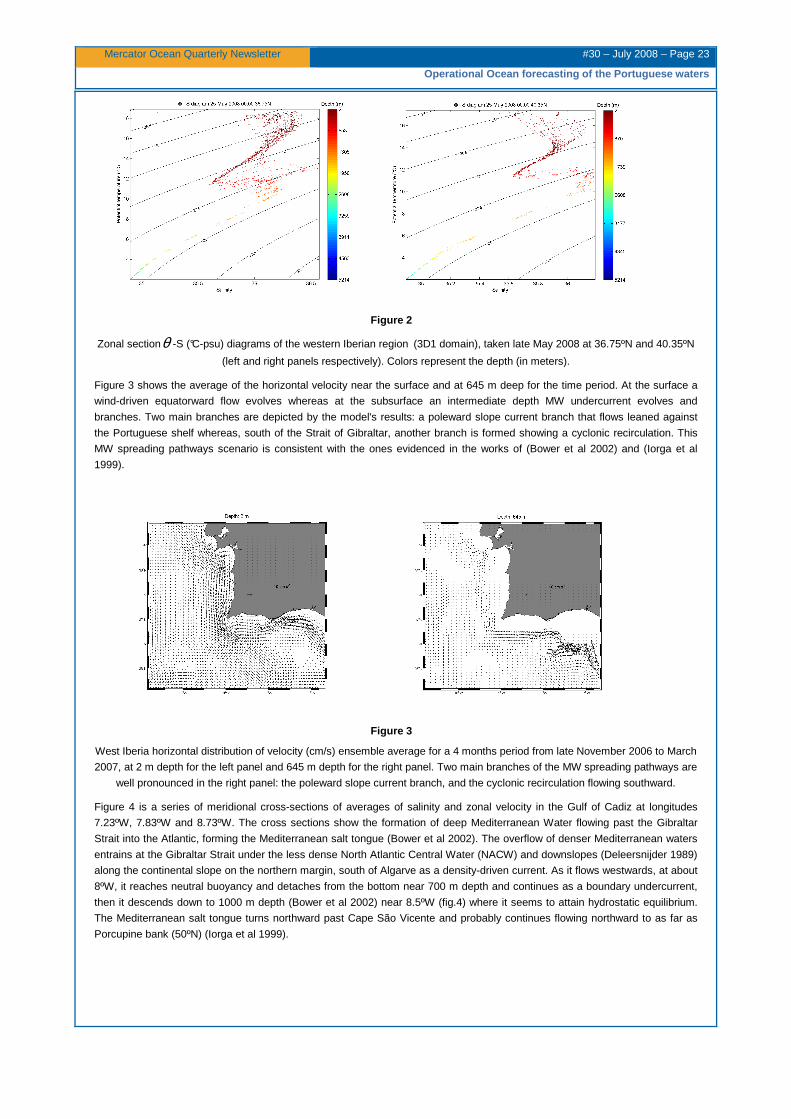
Figure 2

Zonal sectionθ -S (°C-psu) diagrams of the western Iberian region (3D1 domain), taken late May 2008 at 36.75ºN and 40.35ºN

(left and right panels respectively). Colors represent the depth (in meters).

Figure 3 shows the average of the horizontal velocity near the surface and at 645 m deep for the time period. At the surface a

wind-driven equatorward flow evolves whereas at the subsurface an intermediate depth MW undercurrent evolves and

branches. Two main branches are depicted by the model's results: a poleward slope current branch that flows leaned against

the Portuguese shelf whereas, south of the Strait of Gibraltar, another branch is formed showing a cyclonic recirculation. This

MW spreading pathways scenario is consistent with the ones evidenced in the works of (Bower et al 2002) and (Iorga et al

1999).

Figure 3

West Iberia horizontal distribution of velocity (cm/s) ensemble average for a 4 months period from late November 2006 to March

2007, at 2 m depth for the left panel and 645 m depth for the right panel. Two main branches of the MW spreading pathways are

well pronounced in the right panel: the poleward slope current branch, and the cyclonic recirculation flowing southward.

Figure 4 is a series of meridional cross-sections of averages of salinity and zonal velocity in the Gulf of Cadiz at longitudes

7.23ºW, 7.83ºW and 8.73ºW. The cross sections show the formation of deep Mediterranean Water flowing past the Gibraltar

Strait into the Atlantic, forming the Mediterranean salt tongue (Bower et al 2002). The overflow of denser Mediterranean waters

entrains at the Gibraltar Strait under the less dense North Atlantic Central Water (NACW) and downslopes (Deleersnijder 1989)

along the continental slope on the northern margin, south of Algarve as a density-driven current. As it flows westwards, at about

8ºW, it reaches neutral buoyancy and detaches from the bottom near 700 m depth and continues as a boundary undercurrent,

then it descends down to 1000 m depth (Bower et al 2002) near 8.5ºW (fig.4) where it seems to attain hydrostatic equilibrium.

The Mediterranean salt tongue turns northward past Cape São Vicente and probably continues flowing northward to as far as

Porcupine bank (50ºN) (Iorga et al 1999).



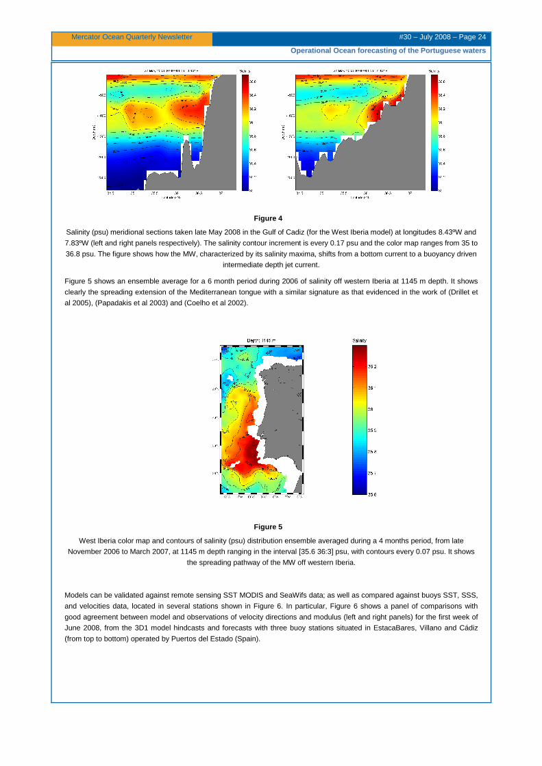
Figure 4

Salinity (psu) meridional sections taken late May 2008 in the Gulf of Cadiz (for the West Iberia model) at longitudes 8.43ºW and

7.83ºW (left and right panels respectively). The salinity contour increment is every 0.17 psu and the color map ranges from 35 to

36.8 psu. The figure shows how the MW, characterized by its salinity maxima, shifts from a bottom current to a buoyancy driven

intermediate depth jet current.

Figure 5 shows an ensemble average for a 6 month period during 2006 of salinity off western Iberia at 1145 m depth. It shows

clearly the spreading extension of the Mediterranean tongue with a similar signature as that evidenced in the work of (Drillet et

al 2005), (Papadakis et al 2003) and (Coelho et al 2002).

Figure 5

West Iberia color map and contours of salinity (psu) distribution ensemble averaged during a 4 months period, from late

November 2006 to March 2007, at 1145 m depth ranging in the interval [35.6 36:3] psu, with contours every 0.07 psu. It shows

the spreading pathway of the MW off western Iberia.

Models can be validated against remote sensing SST MODIS and SeaWifs data; as well as compared against buoys SST, SSS,

and velocities data, located in several stations shown in Figure 6. In particular, Figure 6 shows a panel of comparisons with

good agreement between model and observations of velocity directions and modulus (left and right panels) for the first week of

June 2008, from the 3D1 model hindcasts and forecasts with three buoy stations situated in EstacaBares, Villano and Cádiz

(from top to bottom) operated by Puertos del Estado (Spain).



Figure 6

Location of the buoys from Instituto Hidrográfico (Portugal) and Puertos del Estado (Spain) on the left panel. Sea surface

velocity time series of direction (middle panel) represented by the angle in degrees relative to the geographical North, and

modulus (right panel) in meters per second (m.s-1) taken during the June 3rd 2008 to June 12th 2008 period for the

EstacaBares (top), Villanos-Sisargas (middle) and Cadiz (bottom). The time series represent the buoys data (in red), the West

Iberia model first day forecasts (in blue) and three-day forecasts (in green).



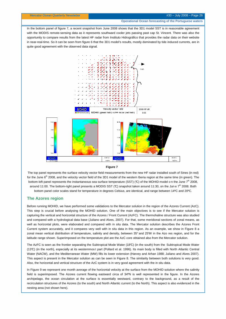
In the bottom panel of figure 7, a recent snapshot from June 2008 shows that the 3D1 model SST is in reasonable agreement

with the MODIS remote-sensing data as it represents southward cooler jets passing past cap St. Vincent. There was also the

opportunity to compare results from the latest HF radar from Instituto Hidrográfico that provides the radar data on their website

in near-real-time. So it can be seen from figure 6 that the 3D1 model’s results, mostly dominated by tide induced currents, are in

quite good agreement with the observed data signal.

Figure 7

The top panel represents the surface velocity vector field measurements from the new HF radar installed south of Sines (in red)

for the June 6th 2008, and the velocity vector field of the 3D1 model of the western Iberia region at the same time (in green). The

bottom-left panel represents the instantaneous sea surface temperature (SST) (°C) of the MOHID model o n the June 7th 2008,

around 11:00. The bottom-right panel presents a MODIS SST (°C) snapshot taken around 11:30, on the Jun e 7th 2008. Both

bottom panel color scales stand for temperature in degrees Celsius, are identical, and range between 14ºC and 20ºC.

The Azores region

Before running MOHID, we have performed some validations to the Mercator solution in the region of the Azores Current (AzC).

This step is crucial before analysing the MOHID solution. One of the main objectives is to see if the Mercator solution is

capturing the vertical and horizontal structure of the Azores / Front Current (AzFC). The thermohaline structure was also studied

and compared with a hydrological data base (Juliano and Alves, 2007). For that, some meridional sections of zonal means, as

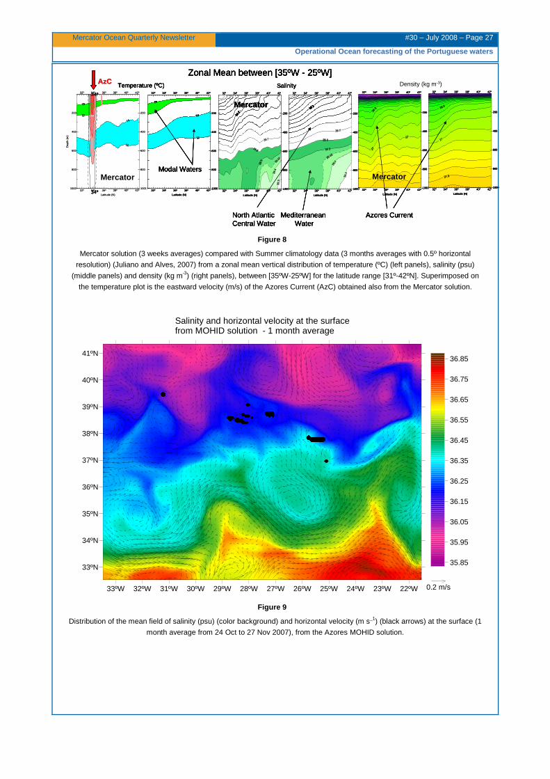
well as horizontal plots, were elaborated and compared with in situ data. The Mercator solution describes the Azores Front

Current system accurately, and it compares very well with in situ data in this region. As an example, we show in Figure 8 a

zonal mean vertical distribution of temperature, salinity and density, between 35° and 25°W in the Azo res region, and for the

latitude range shown. Superimposed on the temperature plot are the AzC core obtained also from the Mercator solution.

The AzFC is seen as the frontier separating the Subtropical Mode Water (18°C) (in the south) from the Subtropical Mode Water

(13°C) (in the north), especially at its westernmos t part (Pollard et al. 1996). Its main body is filled with North Atlantic Central

Water (NACW), and the Mediterranean Water (MW) fills its lower extension (Harvey and Arhan 1988; Juliano and Alves 2007).

This aspect is present in the Mercator solution as can be seen in Figure 8. The similarity between both solutions is very good.

Also, the horizontal and vertical structure of the AzC system is in very good agreement with the in situ data.

In Figure 9 we represent one month average of the horizontal velocity at the surface from the MOHID solution where the salinity

field is superimposed. The Azores current flowing eastward circa of 34ºN is well represented in the figure. In the Azores

archipelago, the ocean circulation at the surface is essentially westward, contrary to the background, as a result of the

recirculation structures of the Azores (to the south) and North Atlantic current (to the North). This aspect is also evidenced in the

nesting area (not shown here).



1000

800

600

400

200

Dep

th (

m)

32º 34º 36º 38º 40º 42º

-1000

-800

-600

-400

-200

32º 34º 36º 38º 40º 42º

Latitude (N)

32º 34º 36º 38º 40º 42º

-1000

-800

-600

-400

-200

32º 34º 36º 38º 40º 42º

Latitude (N)

32º 34º 36º 38º 40º 42º

-1000

-800

-600

-400

-200

32º 34º 36º 38º 40º 42º

Latitude (N)

32º 34º 36º 38º 40º 42º

-1000

-800

-600

-400

-200

32º 34º 36º 38º 40º 42º

Latitude (N)

32º 34º 36º 38º 40º 42º

-1000

-800

-600

-400

-200

32º 34º 36º 38º 40º 42º

Latitude (N)

32º 34º 36º 38º 40º 42º

-1000

-800

-600

-400

-200

32º 34º 36º 38º 40º 42º

Latitude (N)

Mercator Mercator

Mercator

Temperature (ºC) Salinity Density (kg m-3)

Modal Waters

MediterraneanWater

North AtlanticCentral Water

Azores Current

Zonal Mean between [35ºW - 25ºW]

1000

800

600

400

200

Dep

th (

m)

32º 34º 36º 38º 40º 42º

-1000

-800

-600

-400

-200

32º 34º 36º 38º 40º 42º

Latitude (N)

34º

34º

AzCAzC

Mercator1000

800

600

400

200

Dep

th (

m)

32º 34º 36º 38º 40º 42º

-1000

-800

-600

-400

-200

32º 34º 36º 38º 40º 42º

Latitude (N)

32º 34º 36º 38º 40º 42º

-1000

-800

-600

-400

-200

32º 34º 36º 38º 40º 42º

Latitude (N)

32º 34º 36º 38º 40º 42º

-1000

-800

-600

-400

-200

32º 34º 36º 38º 40º 42º

Latitude (N)

32º 34º 36º 38º 40º 42º

-1000

-800

-600

-400

-200

32º 34º 36º 38º 40º 42º

Latitude (N)

32º 34º 36º 38º 40º 42º

-1000

-800

-600

-400

-200

32º 34º 36º 38º 40º 42º

Latitude (N)

32º 34º 36º 38º 40º 42º

-1000

-800

-600

-400

-200

32º 34º 36º 38º 40º 42º

Latitude (N)

Mercator Mercator

Mercator


Modal Waters

MediterraneanWater


Azores Current


1000

800

600

400

200

Dep

th (

m)

32º 34º 36º 38º 40º 42º

-1000

-800

-600

-400

-200

32º 34º 36º 38º 40º 42º

Latitude (N)

34º

34º

AzCAzC

1000

800

600

400

200

Dep

th (

m)

32º 34º 36º 38º 40º 42º

-1000

-800

-600

-400

-200

32º 34º 36º 38º 40º 42º

Latitude (N)

32º 34º 36º 38º 40º 42º

-1000

-800

-600

-400

-200

32º 34º 36º 38º 40º 42º

Latitude (N)

32º 34º 36º 38º 40º 42º

-1000

-800

-600

-400

-200

32º 34º 36º 38º 40º 42º

Latitude (N)

32º 34º 36º 38º 40º 42º

-1000

-800

-600

-400

-200

32º 34º 36º 38º 40º 42º

Latitude (N)

32º 34º 36º 38º 40º 42º

-1000

-800

-600

-400

-200

32º 34º 36º 38º 40º 42º

Latitude (N)

32º 34º 36º 38º 40º 42º

-1000

-800

-600

-400

-200

32º 34º 36º 38º 40º 42º

Latitude (N)

Mercator Mercator

Mercator


Modal Waters

MediterraneanWater


Azores Current


1000

800

600

400

200

Dep

th (

m)

32º 34º 36º 38º 40º 42º

-1000

-800

-600

-400

-200

32º 34º 36º 38º 40º 42º

Latitude (N)

32º 34º 36º 38º 40º 42º

-1000

-800

-600

-400

-200

32º 34º 36º 38º 40º 42º

Latitude (N)

32º 34º 36º 38º 40º 42º

-1000

-800

-600

-400

-200

32º 34º 36º 38º 40º 42º

Latitude (N)

32º 34º 36º 38º 40º 42º

-1000

-800

-600

-400

-200

32º 34º 36º 38º 40º 42º

Latitude (N)

32º 34º 36º 38º 40º 42º

-1000

-800

-600

-400

-200

32º 34º 36º 38º 40º 42º

Latitude (N)

32º 34º 36º 38º 40º 42º

-1000

-800

-600

-400

-200

32º 34º 36º 38º 40º 42º

Latitude (N)

Mercator Mercator

Mercator


Modal Waters

MediterraneanWater


Azores Current


1000

800

600

400

200

Dep

th (

m)

32º 34º 36º 38º 40º 42º

-1000

-800

-600

-400

-200

32º 34º 36º 38º 40º 42º

Latitude (N)

34º

34º1000

800

600

400

200

Dep

th (

m)

32º 34º 36º 38º 40º 42º

-1000

-800

-600

-400

-200

32º 34º 36º 38º 40º 42º

Latitude (N)

34º

34º

34º

34º

AzCAzC

Mercator

Figure 8

Mercator solution (3 weeks averages) compared with Summer climatology data (3 months averages with 0.5º horizontal

resolution) (Juliano and Alves, 2007) from a zonal mean vertical distribution of temperature (ºC) (left panels), salinity (psu)

(middle panels) and density (kg m-3) (right panels), between [35ºW-25ºW] for the latitude range [31º-42ºN]. Superimposed on

the temperature plot is the eastward velocity (m/s) of the Azores Current (AzC) obtained also from the Mercator solution.

33ºW 32ºW 31ºW 30ºW 29ºW 28ºW 27ºW 26ºW 25ºW 24ºW 23ºW 22ºW

Salinity and horizontal velocity at the surfacefrom MOHID solution - 1 month average

33ºN

34ºN

35ºN

36ºN

37ºN

38ºN

39ºN

40ºN

41ºN

35.85

35.95

36.05

36.15

36.25

36.35

36.45

36.55

36.65

36.75

36.85

0.2 m/s

Figure 9

Distribution of the mean field of salinity (psu) (color background) and horizontal velocity (m s_1) (black arrows) at the surface (1

month average from 24 Oct to 27 Nov 2007), from the Azores MOHID solution.



In Figure 10 we compare the sea surface temperature (SST) from MOHID solution with the SST from satellite2 (composite of

microwave and infrared sensors with a ~10 km horizontal resolution) for one day. The microwave data can "see" through the

clouds, a great advantage in the Azores region (contrarily to the high resolution infrared images). This validation is performed

each time the model runs, in an automatic way, producing daily statistics and its evolution during a run. In Figure 11 we present

the evolution of statistical parameters during a run of 35 days (from 24 October to 27 November of 2007), comparing the

solutions of the Mercator and MOHID, with the SST from satellite. The root mean square error (RMSE) and the bias results are

in good agreement with the literature. It was shown that this satellite data agrees well with measured SST taken from buoys and

ships as the comparison between satellite SST and in situ data (buoys and ships) yielded a bias of 0.1 ºC and a RMSE of 0.6

ºC (Wentz et al., 2000; Bhat et al.,2004). The results presented here in the left panel of Figure 11 show a mean bias of 0.1 ºC

and a mean RMSE of 0.6 ºC which is consistent with those from literature.

30ºW 25ºW

SST (ºC) from satellite

35ºN

40ºN

30ºW 25ºW

SST (ºC) from MOHID

18.2 18.7 19.2 19.7 20.2 20.7 21.2 21.7 22.2 22.7 23.2

30ºW 25ºW

T_obs - T_Mohid (ºC)

-1.6 -1.2 -0.8 -0.4 0 0.4 0.8 1.2 1.6

2007-11-16

Figure 10

MOHID SST (°C) compared to satellite OI SST (°C) (s ee text) for the day 2007/11/16 in the Azores region.

2 Microwave OI SST data are produced by Remote Sensing Systems and sponsored by National Oceanographic Partnership

Program (NOPP), the NASA Earth Science Physical oceanography Program, and the NASA REASoN DISCOVER Project. Data

are available at www.remss.com



Figure 11

Leftmost panel: Evolution of statistical parameters; the linear correlation coefficient (R), the bias (ºC) and the root mean square

error (ºC) (RMSE), during 35 days runs, starting on 24 Oct and ending on 27 Nov, 2007, for Mercator solution vs SST satellite

(Blue line) and MOHID solution vs SST satellite (red line). Right panels: T-S diagrams of ARGO float profile data (blue) at

several locations (see figure12 for location of the buoys) and for the time indicated. Superimposed are the Mercator (green) and

the MOHID (red) solutions.

One first inspection to TS multi-plots (Figure 11) of the Mercator solution over the Azores region has shown that there are some

zones near the occidental group of the Azores archipelago without the marked signature of MW, contrasting with the rest of the

Archipelago. A closer inspection of the region shows the topography acting as a barrier to the westward spread of the MW. This

is clearly seen in Figure 12 that represents the MOHID solution of the horizontal distribution of the salinity and velocity at 1000

m depth, in the Azores region. In the western side there is an intrusion of less salty water coming from northwest (associated to

the currents in the region) whereas at the eastern side we see the MW signature, coming from the East (but not associated with

the velocity field, as we can see in the Figure 12). Further analyses and longer time series of model solution are needed to

clarify the possible path of MW in the Azores archipelago (see also Jia et al. 2007). In the same figure we have the positions of

the ARGO floats3 that have been found in the region for the same time period (35 days). We have compared both the Mercator

and the MOHID solutions with the observed data (Figure 11). Besides the fact that both the solutions compare very well with the

in situ data (below the 50 m depth), we can see that the float number 2 corroborates the hypothesis of the topography acting as

a barrier to the westward MW spreading as it shows an absence of MW signal on the TS plot. We also present some other

floats profiles TS diagrams located in other regions, where we can see the MW signal.

3 These data were collected and made freely available by the International Argo Project and the national programs that

contribute to it. (http://www.argo.ucsd.edu, http://argo.jcommops.org). Argo is a pilot program of the Global Ocean Observing

System.



33ºW 32ºW 31ºW 30ºW 29ºW 28ºW 27ºW 26ºW 25ºW 24ºW 23ºW 22ºW

Salinity and horizontal velocity at 1000m depthfrom MOHID solution - 1 month average

33ºN

34ºN

35ºN

36ºN

37ºN

38ºN

39ºN

40ºN

41ºN

12

3

4

5

6

7

8

9

10

11

12

13

14

15

16

17

18

19

20

21

22

23

24

25

26

27

28

29

30

31

32

33 35.15

35.25

35.35

35.45

35.55

35.65

35.75

35.85

35.95

0.1 m/s

Figure 12

Same as Figure 9 but for 1000 m depth. The white circles represent the locations of the ARGO floats profile data (see the text

for references) found in the Azores region during the period 24 Oct to 27 Nov 2007

Concluding Remarks

The generic nesting technique of the M-O solution that adds the tide signal, and was first devised by (Leitão et al 2005), can be

applied to any domain region and yet yields interesting results. While the quality assessment of the forecasts still requires a lot

of work, we have realistic results for processes like the MW spreading, the tide, and the θ -S signature of the main water

masses is in good agreement with observed data (Fiúza et al 1998). The MOHID model can provide new insights in regions

where realistic finer-scale models were not previously run as it was shown for the case of the Azores region. It can be used as a

forecasting tool, and what it lacks in speed, it gains in versatility and extensibility with its suite of water-quality and

biogeochemical models, of which a few sample applications can be seen in (Trancoso et al 2005) and (Saraiva et al 2007).

On-going and future work

The on-going work related with the implementation of an operational forecasting system in Portuguese waters is following three

main pathways: verify the accuracy of the present model configuration, improve the MOHID operational capabilities and closing

the gap between the scientific modelling community and the end users. The model accuracy is being quantified comparing the

model results with satellite data (SST), Argo floats, buoys data and recently with HF-radar data. Another way of assessing the

model performance is participating in numerical model intercomparison exercises like the one underway for the Bay of Biscay

for the year 2004. In this case the NEMO-OPA, HYCOM, SYMPHONIE, MARS and MOHID model results forced with the same

boundary conditions are being compared (see companion article by Reffray et al., this issue). The MOHID model operational

capabilities are being expanded. Two new MOHID assimilation modules are now in the testing phase, one based in Kalman

filtering (e.g. SFEK, SEEK) which mainly focuses on the assimilation of remote sensing and buoy data in coastal waters and

another based on the (Cooper and Haines 1996) method focussing on assimilating altimetry in off-shore waters. Finally, the

development of a framework is underway, that allows in an efficient manner to do one-way nesting of high resolution numerical

model applications from large scale models such as Mercator Ocean solutions. This framework will allow building quickly

realistic hydrodynamical models of any regional or local domain. In a first phase, this system will exclusively be based on the

MOHID model but in the future, this framework will be used to nest other operational systems and other models. The concept is

already being tested in several projects along the Portuguese coast to support local operational services.



Acknowledgements

The authors wish to thank the Mercator Ocean team for providing the ocean forecasts and the reanalysis, Meteo-IST (in

particular J. J. Delgado Domingos and A. Rosa Trancoso) and Ricardo Tomé for providing the atmospheric forecasts. The

authors wish also to thank Puertos Del Estado for providing us with real-time buoys data. G. Riflet also wishes to thank warmly

all the fruitful conversations with Nathalie Verelst on the water masses found off western Iberia. This work is co-funded by the

EU in the framework of INTERREG III-B Espaço-Atlântico activities in the scope of the EASY project. The website is available at

http://project-easy.info. G. Riflet acknowledges grant SFRH/BD/17631/2004 from Fundação para a Ciência e Tecnologia. The

authors wish also to thank the revision of Laurence Crosnier for relevant contributions to the clarity of this work.

References

Bhat, G.S., Vecchi, G.A. and Gadgil, S. 2004: Sea surface temperature of the Bay of Bengal derived from the TRMM

Microwave Imager. J. Atmos. Ocean. Technol. 21:1283–1290.

Blayo, E., L. Debreu. Revisiting open boundary conditions from the point of view of characteristic variables. Ocean Modelling,

9:231-252, 2005.

Blumberg, A. F., L. H. Kantha. Open Boundary Condition for Circulation Models. Journal of Hydraulic Engineering, 111(2):237-

255, 1985.

Bower, A. S., Serra, N., Ambar, I., 2002. Structure of the mediterranean undercurrent and mediterranean water spreading

around the southwestern iberian peninsula. Journal of Geophysical Research 107 (C10).

Chelton, D. B., R. A. Deszoeke, M. G. Schlax, El K. Naggar, and N. Siwertz. Geographical variability of the first baroclinic rossby

radius of deformation. Journal of Physical Oceanography, 28(3):433-460, 1998.

Coelho, H. S., R. J. J. Neves, M. White, P. C. Leitão, and A. J. Santos. A model for ocean circulation on the iberian coast.

Journal of Marine Systems, 32(1):153-179, 2002.

Cooper, M., Haines, K., 1996. Altimetric assimilation with water property conservation. J. Geophys. Res. 101, 1059-1078.

Deleersnijder, E.. Upwelling and upsloping in three-dimensional marine models. Applied Mathematical Modelling, 13:462-467,

1989.

Domingos, J. J. Delgado, A. R. Trancoso. Meteo-ist. Internet service, 2005.

Doty, B. E., J. Wielgosz, J. Gallagher, and D. Holloway. GrADS and DODS/OPENDAP. Proceedings of the 17th International

Conference on Interactive Information and Processing Systems (IIPS) for Meteorology, Oceanography, and Hydrology,

American Meteorological Society Albuquerque, NM, 385, 2001.

Drillet, Y., Bourdalle R. Badie, L. Siefridt, and C. Le Provost. Meddies in the Mercator North Atlantic and Mediterranean Sea

eddy-resolving model. Journal of Geophysical Research, 110(C3), 2005.

Etopo, N.. Bathymetry. Product Information Catalogue, see also http://www.ngdc.noaa.gov/mgg/global/seltopo. html, 1988.

Fiúza, A. F., Hamann, M., Ambar, I., Diaz, Gonzalez, N., Cabanas, J. M., July 1998. Water masses and their circulation off

western iberia during may 1993. Deep Sea Research Part I: Oceanographic Research Papers 45 (7), 1127-1160.

Flather, R. A. A tidal model of the northwest European continental shelf. Mem. Soc. R. Sci. Liege, 10(6):141-164, 1976.

Iorga, M. C., M. S. Lozier. Signatures of the Mediterranean outflow from a North Atlantic climatology 1. Salinity and density

fields. Journal of Geophysical Research, 104(C11):25985-26010, 1999.

Harvey, J., and M. Arhan, 1988: The water masses of the central North Atlantic in 1983–84. J. Phys. Oceanogr., 18, 1855–

1875.

Jia, Y., A.C. Coward, B.A. de Cuevas, D.J. Webb, and S.S. Drijfhout, 2007: A Model Analysis of the Behavior of the

Mediterranean Water in the North Atlantic. J. Phys. Oceanogr., 37, 764–786.

Juliano, M.F., and M.L.G.R. Alves, 2007: The Atlantic Subtropical Front/Current Systems of Azores and St. Helena. J. Phys.

Oceanogr., 37, 2573–2598.

Leitão, P. , H. Coelho, A. Santos, and R. Neves. Modelling the main features of the Algarve coastal circulation during July

2004: A downscaling approach. Journal of Atmospheric and Ocean Science, 10(1) :421-462, 2005.

http://project-easy.info



Lyard, F., F. Lefevre, T. Letellier, and O. Francis. Modelling the global ocean tides: modern insights from fes2004. Ocean

Dynamics, 56(5-6):394-415, December 2006.

Martinsen, E. A., H. Engedahl. Implementation and testing of a lateral boundary scheme as an open boundary condition in a

barotropic ocean model. Coastal engineering, 11(5-6):603-627, 1987.

Papadakis, M. P., E. P. Chassignet, and R. W. Hallberg. Numerical simulations of the mediterranean sea outflow: impact of the

entrainment parameterization in an isopycnic coordinate ocean model. Ocean Modelling, 5(4):325-356, 2003.

Pollard, R. T., M. J. Griffiths, S. A. Cunningham, J. F. Read, F. F. Perez, and A. F. Rios, 1996: Vivaldi 1991- A study of the

formation, circulation and ventilation of eastern North Atlantic Central Water. Prog. Oceanogr., 37, 167–192.

Riflet, G., Leitão, P. C., Fernandes, R., Neves, R., April 2007. Assessing the quality of a pre-operational model for the

portuguese coast. In: European Geosciences Union 2007. No. 09979 in 1607-7962/gra/EGU2007-A-09979.

Saraiva, S., Pina, P., Martins, F., Santos, M., Braunschweig, F., Neves, R., 2007. Modelling the influence of nutrient loads on

portuguese estuaries. Hydrobiologia 587 (1), 5-18.

Stevens, I., M. Hamann, J. A. Johnson, and A. F. G. Fiúza. Comparisons between a fine resolution model and observations in

the iberian shelf-slope region. Journal of Marine Systems, 26(1):53-74, 2000.

Wentz, F.J., Gentenmann, C., Smith, D. and Chelton, D. 2000: Satellite measurements of sea surface temperature through

clouds. Science 288:847–850.

Trancoso, A., Saraiva, S., Fernandes, L., Pina, P., Leitão, P., Neves, R., 2005. Modelling macroalgae using a 3 d

hydrodynamic-ecological model in a shallow, temperate estuary. Ecological Modelling 187 (2), 232-246.


PREVIMER: Operational MARS syste m in the Bay of Biscay

PREVIMER: Operational MARS system in the Bay of Bis cay By Fabrice Lecornu, Pascal Lazure, Valérie Garnier, Alain Ménesguen, Marc Sourisseau

Ifremer/ Dyneco, BP70, 29280 Plouzané, France

Introduction

This paper presents the operational MARS system in the Bay of Biscay, implemented within the PREVIMER project. This project

aims at providing a wide range and ever-growing number of coastal area users with observations, modelling tools and real-time

forecasts, taking into account the statutory context. All the operational developments and their implementations are carried out

in the framework of partnership agreements between public institutions (the French public institute for marine research (Ifremer),

the French Naval Hydrographic and Oceanographic Service (SHOM), the French National Weather Service (Météo-France), the

French public science and technology research institute (IRD), the European Institute of Marine Studies (IUEM)) and private

companies (R&D departments, small to medium-sized companies manufacturing oceanographic instruments). The PREVIMER

project is listed within the “Five-year plan drafted between the State and the region, i.e. Brittany, for 2000-2006” which will be

renewed until 2012.

The PREVIMER project is based on observations and coastal ocean modelling. The www.previmer.org website displays

forecasts of current strength and direction, wave height and direction of propagation, sea levels, storm surges, temperature,

salinity, nutrients and phytoplankton concentrations along the French coastline. These data and their analyses will provide

essential information for coastal zone usage or management. A special focus is put on the modelling tool at the scale of the Bay

of Biscay.

Bay of Biscay modelling

Hydrodynamical model

The operational hydrodynamical model MARS has recently been enlarged to encompass both the Bay of Biscay and the English

Channel. A recent paper (Lazure et al., 2008) gives a full description of the operational model and its validations against

hydrological data in the Bay of Biscay. A brief summary of the model characteristics and its validation is given here. The model

extends from 8°W to the Dutch coast in the North Se a and from the Spanish coast to 52°45’N. The horizo ntal resolution is of 4

km, 30 vertical levels are considered and refined near the surface.

The kernel of the MARS model has been fully described by Lazure and Dumas (2008). This finite difference model operates on

a regular horizontal grid and sigma coordinates along the vertical. It is a mode splitting model with an original coupling of the

barotropic-baroclinic modes. The barotropic component of the open boundary conditions (i.e. the effects of tide and pressure

induced circulation) is obtained by a wider model, that extends from 20°W to 10°E in longitude and fro m Portugal to Iceland in

latitude and that is forced by winds, atmospheric pressure and tides (FES2004 data basis, Lyard et al., 2006) at the open

boundaries. Analysed fields of wind and pressure are issued from the model ARPEGE of the French Meteorological office

(Météo-France). Baroclinic boundary conditions (temperature, salinity, free surface elevation and currents) for hindcast are

provided by global ORCA025 (A.M. Tréguier and V. Thierry, pers. com.) solution which is very similar to the model described by

Barnier et al. (2006). For operational applications, the boundary conditions are climatological data yet. The use of real time

Mercator solution (PSY2V3, Atlantic system with 1/12° resolution) at the open boundary is planned befo re the end of 2008. The

run offs of 27 rivers are imposed in the estuaries. The 4 main rivers (Adour, Gironde, Loire and Vilaine) account for more than

90% of the total input in the Bay of Biscay, their discharges are measured daily (French freshwater office database,

http://www.hydro.eaufrance.fr). Climatological data are prescribed for the other rivers.

Tidal dynamics in the Bay of Biscay has been evaluated (Lazure and Dumas, 2008): the tide is accurately simulated and

comparison with currents profiles records are in acceptable agreement for short time ranges.

The validation of the simulated hydrology over the shelf of the Bay of Biscay has been presented recently (Lazure et al., 2008).

The main results can be summarized as follow: the model reproduces accurately observed salinities both from a climatological

and time evolution point of view along the coast: the transient decays of salinity due to floods of the main rivers are properly

reproduced both in time and magnitude (figure 1).

www.previmer.org



Figure 1

Comparison between measured salinity(psu) (dotted line) at the coast (North of Oleron Island) and predicted salinity(psu)(solid

line).

Figure 2 shows the statistics of comparisons between in situ and predicted salinity over the shelf at several levels during spring.

Over the shelf, the magnitude of salinity compares very well with data: no bias is observed, and the error remains low at the

surface, where the salinity variability develops. The strong decrease of the measured salinity in September 2004 is likely to be

due to a failure of the probe. During that period, the discharges of the main rivers remain very low as usually at the end of

summer. The main discrepancy is related to the summer situation, the model predicts slightly lower salinity than observed near

the coast. The turbulence parameterization (k equation and mixing length prescribed according to the Gaspar et al. (1990)

formulation) is suspected to be the primary cause of this gap between prediction and observation. An increase of the mixing of

the surface layer in summer could lead to an increase of surface salinity.

Figure 2

Statistical comparison of observed and predicted salinities (psu) at different vertical locations during spring. Upper panel:

number of available observations. Mid panel: mean error (psu) .Lower panel: RMS error (psu).

A good global agreement in reproducing SST has been reached. Figure 3 gives an illustration of the predicted temperature and

the SST observation during the same period of time. The model results are shaded over the deep Bay of Biscay and along the

Spanish coast because the results were not validated. As shown in this paper and in Lazure et al. (2008), the validation is under

progress and the results over the whole domain will be soon presented.



Figure 3

SST (°C) averaged over 4 days measured by satellite (left panel). Predicted surface temperature (°C) (right panel).

A qualitative comparison with climatology shows that the model reproduces accurately the main thermal structure over the shelf,

namely: Ushant tidal front, cold bottom pool from spring to autumn, upwellings along the Landes coast in summer and cold

coastal strip in winter and early spring associated with strong river discharges.

However, over the shelf, a global overestimation of the temperature from surface to the bottom is shown both by comparisons

with climatology, in situ and satellite measurements. The overall bias with in situ observation is close to 0°C in spring and

reaches 0.8°C during autumn at the surface. The RMS errors (RMSE) are around 1°C in the first 20m in s pring and around

0.7°C in autumn. The increase of RMSE near the pycn ocline (20m in spring and 40m in autumn) reveals some trouble in

reproducing adequately the stratification.

The comparison with monthly averaged SST satellite during 5 years (1999-2004) shows that the model behaves better during

the onset (spring) than during the breakdown (autumn) of the thermal stratification (Figure 4). During spring the percentage of

predicted temperature which lies between the precision of observations (-0.5, +0.5°C) can reach 85% ov er the whole domain

including the deep Bay of Biscay. This percentage falls down to 50-60% during autumn.

Figure 4

Comparison between SST prediction and observation in percentage of total pixel number over the whole domain. Positive shift

represents the percentage of pixel where the predicted temperature is higher than 0.5°C from the obser vation. Negative shift

when model is cooler.

Primary production model

The 3D model of the pelagic ecosystem of the Bay of Biscay continental shelf, based on the MARS model for hydrodynamics,

has been previously calibrated (Loyer, 2001 and Huret et al., 2007) and turned into an operational real-time mode. For the time

being, the model domain is so far restricted to the Bay of Biscay and the entrance of the English Channel and will be extended

to the whole Channel and south North Sea before the end of the year 2008. A recent paper (Ménesguen et al., 2008) gives the

description of the model and its validation for chlorophyll estimates. The biogeochemical model contains 13 state variables,

describing the nitrogen (N), phosphorus (P) and silicon (Si) cycles in the pelagic ecosystem. Three limiting dissolved inorganic

nutrients are considered: nitrogen, with nitrate and ammonium separately, phosphorus, and silicon. The biological boundaries

conditions (N, P and Si) are climatological data (WOA05, Garcia et al. 2006). Phytoplankton is divided into 3 groups: diatoms,

dinoflagellates and nanoflagellates, with concentrations expressed in nitrogen currency. There are two zooplanktonic

components, expressed in carbon units: the microzooplankton, which eats nanoflagellates and detrital particulate matter, and



the mesozooplankton, which eats diatoms exclusively. In this model, diatoms do sink and are eaten, nanoflagellates and

dinoflagellates do not sink (they are considered as able to maintain their location at any depth thanks to motility) and

dinoflagellates are considered to avoid predation. Three particulate detrital variables (detrital N, detrital P, detrital Si) close the

biogeochemical cycles. On the annual mean basis, the model provides a realistic geographical distribution of phytoplanktonic

biomass (Figure 5). On the time axis, the overall daily mean of simulated chlorophyll exhibits realistic blooms, but remains too

low on the whole domain in winter time, and also in spring and summer in the shallow coastal strip.

Figure 5

Mean annual maps of surface chlorophyll (µg.l-1 ) for 2007 (left: model result, right: MODIS remotely sensed data)

Daily forecasts for the following 2 days are put on the PREVIMER internet server

(http://www.previmer.org/previsions/production_primaire/modele_eco_mars3d_gascogne), for inorganic nutrients (NH4, NO3,

PO4, Si (OH)4) and 3 kinds of phytoplankton (diatoms, nanoflagellates and dinoflagellates) together with the corresponding total

chlorophyll concentration, in the surface and bottom layers.

Concluding remarks and future works

The briefly presented MARS system applied to the Bay of Biscay and the English Channel for hydrodynamics is run daily and

provides forecast for the two coming days. The results have been validated with the comparison to past measurements. The

biological application limited to the French continental shelf of the Bay of Biscay has proved its ability at reproducing the main

chlorophyll patterns over the shelf. The PREVIMER project is not restricted to the western sea front, it also covers the

Mediterranean coast where a high resolution model (grid size: 1.2km, 30 levels) has been developed.

The 2 above seafront hydrodynamical and biological models support the downscaling to local scales. Some applications need

high resolution models which are forced at their boundaries by the seafront models. As an example, a high resolution model

dedicated to the primary production around Brittany is under development and will be available in summer 2008. High resolution

models (mesh size of around 150-300m) of the Bay of Brest, Iroise Sea, Normandy coast, Arcachon basin are also embedded in

the seafront models.

Several developments are under progress to continuously improve the accuracy of the hindcast, nowcast and forecast products:

The MARS model is also being developed: a generalized sigma coordinate system will be soon available and a more general

turbulence closure scheme will be tested to improve the predicted vertical structure of the water column. Some new processes

like wave current interactions will also be considered. Wave forecasting is also calculated by SHOM within PREVIMER project,

the influence of waves on the transport over the shelf is currently being assessed.

http://www.previmer.org/previsions/production_primaire/modele_eco_mars3d_gascogne



Moreover, an EnKF-based data assimilative system of SST is under progress. First assessment has been carried out in spring

and summer and has given substantial improvements for temperature and salinity vertical structure over the shelf. The efficiency

of combined parameter and state estimation to reduce the SST model forecast biases over the shelf has been also shown over

April-May, a period for which the forecast error is mainly governed by the extinction coefficient which accounts for the water

transparency and the penetration of solar flux. Operational implementation is due to occur in 2009.

As the PREVIMER project unfolds, we will be able to deploy a more comprehensive strategy for more frequent observations of

our coastal seas, with a higher spatial resolution: we will improve measurement networks - measuring more parameters,

especially for biology, and using real-time transmission.

A bi monthly newsletter of PREVIMER products is published, targeting a large public. It provides a description of the main

parameters (SST, salinity, primary production, waves….) averaged by month, and their anomalies with respect to their

climatological values. The main meteorological (severe storm) or oceanographical events (strong flood, extreme waves …) are

also highlighted.

Lastly, the PREVIMER products in a near future will become more comprehensive and of higher quality, while remaining

generic. Ensuring the lastingness of their production could grow a downstream commercial field, based on highly specialized

services. A website remaining active and attentive to users' comments is also a guarantee for constant progress.

References

Barnier, B., G. Madec, T. Penduff, J.M. Molines, A.M. Treguier, J. Le Sommer, A. Beckmann, A. Biastoch, C.B¨oning, J. Dengg,

C. Derval, E. Durand, S. Gulev, E. Remy, C. Talandier, S. Theetten, M. Maltrud, McClean, B. De Cuevas 2006: Impact of partial

steps and momentum advection schemes in a global ocean circulation model at eddy permitting resolution. Ocean Dynamics,

DOI: 10.1007/s10236-006- 0082-1.

Garcia, H. E., R. A. Locarnini, T. P. Boyer, and J. I. Antonov, 2006. World Ocean Atlas 2005, Volume 4: Nutrients (phosphate,

nitrate, silicate). S. Levitus, Ed. NOAA Atlas NESDIS 64, U.S. Government Printing Office, Washington, D.C., 396 pp.

Gaspar J.P., Grégoris U., Lefèvre J.M. 1990. A simple eddy kinetic energy for simulations of oceanic vertical mixing : test at

station papa and long term upper ocean study site. Journal of Geophysical Research, 95 (C9), 16179-16193.

Huret, M., F. Gohin, D. Delmas, M. Lunven, V. Garçon, 2007. Use of SeaWiFS data for light availability and parameter

estimation of a phytoplankton production model of the Bay of Biscay. Journal of Marine Systems, 65(1-4): 509-531.

Lazure P., Dumas F., 2008. An external–internal mode coupling for a 3D hydrodynamical model for applications at regional

scale (MARS). Advances in Water Resources, 31(2), 233-250.

Lazure, P., Garnier, V., Dumas, F., Herry, C., Chifflet M. 2008. Development of a hydrodynamical model of the Bay of Biscay.

Validation of hydrology. Cont. Shelf. Res. Submitted.

Lyard, F., Lefevre, F., Letellier, T., and Francis, O., 2006. Modelling the global ocean tides: modern insights from FES2004.

Ocean Dynamics, 56:394–415, doi:10.1007/s10236-006-0086-x.

Loyer, S., 2001. Modélisation de la production phytoplanctonique dans la zone côtière atlantique enrichie par les apports

fluviaux. Ph. D. thesis, Université de Paris VI, 232 pp.

Ménesguen A, Baey J.M., Sourisseau M., 2008. Real time ecological modelling of nutrients and phytoplankton of the Bay of

Biscay French Shelf. Cont., Shelf. Res. Submitted.

.


Keys to affordable regional marine forecast systems

Keys to affordable regional marine forecast systems By Patrick Marchesiello 1, Jérôme Lefèvre 1, Pierrick Penven 2, Florian Lemarié 1, Laurent Debreu 3,

Pascal Douillet 1, Andres Vega 1, Patricia Derex 1, Vincent Echevin 4 and Boris Dewitte 5 1 IRD/LEGOS/UR065, IRD Noumea, Centre BPA05, 98848 Noumea Cedex, Nouvelle Caledonie. 2 IRD/UR097, ECO-UP, Centre IRD de Bretagne, B.P. 70, 29280 Plouzane, France 3 INRIA, 51 rue des mathémathiques, B.P. 53, 38041 Grenoble, France 4 IRD/LOCEAN, Institut Pierre Simon Laplace, Boîte 100 - 4, place Jussieu 75252 PARIS Cedex 05, France 5 IRD/LEGOS/IMARPE, Esquina de Gamarra y General Valle S/N Chucuito, Callao, Peru

Introduction

Only the wealthiest countries in the world can propose governmental services with decent financial support to provide marine

forecasting on an operational level. If a laboratory of oceanography or meteorology in a developing country needs to provide

marine forecast to support its country’s economy or prevent pollution, what alternative can be found? This is precisely the kind

of questions that the Institute of Research for Development (IRD) is designed to answer.

Figure 1

The oceanographic research group at the Nouméa-IRD center proposes a functional but experimental nowcast/forecast

integrated system of marine meteorology, deep sea and lagoon oceanography which is updated everyday through the web

site: http://prevision.ird.nc

http://prevision.ird.nc



Our understanding is that a regional marine forecast system needs at its core some state-of-the-art regional oceanic and

atmospheric models which can be applied in a downscaling mode to refine the results of existing global systems, rather than

generating entirely new solutions. The challenge is to find freely available models and global operational data sets, then build

interfaces extracting these data, interpolate it to the regional grids, integrate the models in both nowcast and forecast modes,

analyze the results and present them to potential users through a distributed media (the World Wide Web). A key condition for

our system to work is that maintenance be minimal, which can only be achieved if the system is entirely automated through

scheduled commands and scripts.

With support from the PREVIMER project, as well as IRD (Institut de Recherche pour le Développement), ANR (Agence

Nationale de la Recherche) and ZoNéCo (New Caledonia government research program), an experimental but fully automated

system was created for marine survey and forecast of the New-Caledonia region (http://prevision.ird.nc ; Figure 1). New

Caledonia is well suited for the experiment because it gathers most of the constraints encountered in developing countries, i.e.

slow internet connection, remoteness from data centers, expensive or unavailable hardware and software. Meanwhile, good

research conditions at the IRD-Nouméa center and a comfortable financial support has provided the means to explore different

paths and reach the experiment’s goal. In a second phase, the experimental system should be exported towards developing

countries. This step is underway as parts of the system are already active in Peru, Mexico, Senegal and South Africa.

The marine forecast system of New-Caledonia is rather complex as it comprises 3 parts: the oceanic, the lagoon and the

atmospheric models (Figure 2). In the following we present those different parts, emphasizing key points that are relevant to a

portable and affordable operational system.

Hardware

Recent modeling developments have greatly benefited from the rapid progress of Personal Computers, including hardware,

operating systems, libraries and compilers. Those in turn are largely profiting from the free software era in which we now evolve.

As a result, multiple processor machines are so efficient that single-core, single-processor machines are not found on the

market anymore. Therefore, oceanic and atmospheric modeling is unconceivable without code parallelization, which can

simultaneously use multiple cores of one processor, or/and multiple processors of one PC, or/and multiple PCs of a cluster.

Under these circumstances and because our models are efficiently parallelized, we have found support during the last 3 years

to progressively build an experimental PC cluster in Noumea for scientific computing (Figure 3); our objective is to demonstrate

that a cheap and efficient local-size machine (40 processor units) can be built in developing countries. In this experiment, we

have learned that all necessary computer software (operating system, cluster administration system, communication libraries,

compilers, job manager system) is freely available and functional, provided that a few options are properly set. The

performances of local-size PC clusters can be excellent, although it shows a few bottle necks such as dual-core parallelization

(there is efficiency loss using message passing protocols on a dual-core processor compared to a bi-processor, but the loss has

been found acceptable) and more importantly the PCs connection system. A high communication bandwidth capability appears

indispensable when the number of grid points exchanging information becomes large compared to the total grid points (with

slow connection, the volume of data transfer becomes too large compared to actual computing). Therefore, our choice went to

the InfiniBand connection (10Gbps of bandwidth) which allows using the full cluster capacity even on computational grids that

LAGOONMARS3D ROMS ADCIRC

Regional OCEANROMS

Regional METEOWRF

Global OCEANMERCATOR

Global surface METEOGFS

Global METEOGFS

Global TIDESTPXO

LAGOONMARS3D ROMS ADCIRC

Regional OCEANROMS

Regional METEOWRF

Global OCEANMERCATOR

Global surface METEOGFS

Global METEOGFS

Global TIDESTPXO

Figure 2

Diagram presenting the different parts of the IRD integrated operational system. Extraction and transfer from global (green)

to regional (yellow) stages are done using the OPeNDAP extraction protocol; each step is completely automated through

the Linux CRON service. It takes about 2 hours every night for the entire system to run on 4 processors.

http://prevision.ird.nc



are relatively small. Based on the lessons learned and selected choices, a similar PC cluster is now being implemented in Lima

(Peru) as a second phase of the experiment.

The oceanic system

This section only concerns the oceanic system at the regional scale (Figure 2). The lagoon of New Caledonia, which is an

isolated body of water with limited connections to the ocean, is treated in the section below “Coupling”.

Model and configurations

The Regional Ocean Modeling System (ROMS) is a new generation ocean circulation model (Shchepetkin and McWilliams,

2005). It has been specially designed for the accurate simulation of regional oceanic systems with coastal margins. IRD jointly

with INRIA (Institut National de Recherche en Informatique et en Automatique) are maintaining a separate branch of the model

(ROMS_AGRIF) which features multi-level 2-way nesting capability (Penven et al., 2006), and a modified code structure to

straightforwardly handle realistic modeling and its application modules. The conjunction of a stable, accurate and efficient model

with robust open boundary conditions (Marchesiello et al., 2001) allows us to follow a systematic approach to obtain a

“standard” regional configuration (Marchesiello et al., 2003). To that end, a series of MATLAB routines and several essential

datasets were gathered in an integrated toolbox called ROMSTOOLS (Penven et al., 2007; the toolbox and the model can be

freely downloaded at: http://www.brest.ird.fr/Roms_tools/). ROMSTOOLS requires only a minimum list of elements (location and

size of parent and nested domains, resolutions …) to obtain a model simulation for almost any region. The standard pre-

processing tools include interpolation procedures, generic land masking and topography smoothing. Refinements are then

added as needed, i.e. nested domains, more accurate wind forcing, initial, boundary and topographic data, as well as various

biogeochemical data for relevant applications. In various complex configurations, ROMSTOOLS and ROMS_AGRIF have been

applied successfully on a variety of regional studies of the world ocean (Blaas et al., 2007; Blanke et al., 2002; Capet et al.,

2004; Karakas et al., 2006; Gruber et al., 2006; Marchesiello et al., 2003, 2007; Messie et al., 2006; Peliz et al., 2007ab;

Penven et al., 2000, 2006; among others). Note that ROMSTOOLS should evolve in the future towards free programming

languages replacing MATLAB (OCTAVE for example) in order to better comply with our portability-affordability constraint.

The configuration of the New Caledonia region which is currently used for daily forecasts is built on a 1/6° resolution grid

encompassing the whole southwest Pacific. A nested domain for grid refinement (5 km) over the New Caledonia Exclusive

Economic Zone has been implemented and tested (Figure 4 and section below ”A low-cost observatory for survey and

validation”), and should be operational in a future system upgrade.

Figure 3

Nouméa PC cluster, made of 10 bi-dual-core Opteron processor 246 and 285, with motherboard Tyan S2885 and Infiniband

connection for communication between the PCs. The Cluster was assembled at the IRD-Nouméa center.

http://www.brest.ird.fr/Roms_tools/



Forecast_tools

The impact of climate change on the coastal oceans and operational oceanography are two of the highlights of modern

oceanography. ROMSTOOLS allows running both inter-annual and real-time simulations. In the latter case, we rely on

operational global ocean circulation models for the initial and lateral boundary conditions and operational global atmospheric

models (introduced through bulk formulations) for surface forcing. Alternatively, we can use a regional atmospheric model to

provide small-scale surface forcing data (cf. section below “The atmospheric system” and Figure 2).

In order to limit the volume of data transferred over the Internet, we use the Open-source Project for a Network Data Access

Protocol (OPeNDAP) and extract only the necessary subgrid. This method reduces by a great amount the bandwidth needed for

data download. This point is critical for laboratories which do not have access to a high performance Internet connection.

Another critical point of the same type is the availability of data. It should be acknowledged that U.S. data bases are far more

interesting in this respect than European ones, although the efforts made by Mercator (partly under IRD’s demand) to provide its

quarter-degree resolution forecast product through an OPeNDAP server is encouraging.

If large scale ocean dynamics are slow in comparison with those of the regional system (this might be incorrect near rapidly

changing large scale systems such as western boundary currents), the lateral boundary conditions can be interpolated from a

coarse-resolution operational model. The issue of the global model resolution becomes more sensitive when considering the

initialization problem. In a regional domain with low intrinsic variability where the circulation is directly forced by surface fluxes

(for example in the nearshore zone of coastal upwelling regions; or in the deep sea regions away from fronts and eddies),

initialization is of lower importance (a restart file created at a given forecast cycle can be used for the next cycle). In this case,

ocean circulation predictability is relying on that of the forcing fields. Those are generated using extracted data from the half-

degree, 6-hourly Global Forecast System (GFS), freely available via OPeNDAP by the U.S. National Center for Environmental

Prediction (NCEP/NOAA). Higher resolution winds from our regional atmospheric model can also be used, as in the lagoon

component of the system (See sections below “The atmospheric system” and “Coupling”).

Figure 4

ROMS embedded in Mercator Ocean. Over New Caledonia EEZ, a fine grid at 5km resolution is nested in the parent ROMS

domain at 1/6°. Top: model SST for January 30, 2003 . Bottom: comparison of model temperature at 30 m with Uitoé station.

The problem becomes more complicated if oceanic intrinsic variability is dominant. In this case, mesoscale eddies, with

dynamics evolving at a time-scale of the order of the month, are generated on a regular basis and have low predictability. The

model may well provide a very statistically reliable image of the mesoscale dynamics (Marchesiello et al., 2003), but eddies at



any given time are usually not correlated with real events. An initialization method is therefore needed to adjust the statistically

reliable oceanic variable to the real time. To that end, a now widely used method is data assimilation. For our nested version of

ROMS, a three-dimensional variational system called ROMS_DAS (Li et al., 2008) was developed at the Jet Propulsion

Laboratory during a collaborative project involving UCLA (some of the authors, now at IRD, participated in this project). The

project called AOSNII consisted in evaluating an adaptive ocean sampling design (Chao et al., 2003), where observations and

model solutions regularly interact in order to optimize the survey sampling. Despite the good performances shown, ROMS_DAS

has not yet been incorporated in the New Caledonia operational experiment. Instead, we have opted for an alternative method,

which makes use of Mercator’s new quarter-degree resolution forecast product. The global product in this case assimilates for

us real-time mesoscale eddies from satellite altimetry and in-situ data. Then, Newtonian nudging is used to adjust Mercator data

to ROMS dynamics. The nudging is performed during the nowcast step, and a few iterative cycles can be done to guarantee

convergence of the resulting nowcast field (for example when first starting up the operational system).

The strategy for a nowcast/forecast cycle is as follows. A first week of simulation (from t0-7 to t0, t0 being the present time) in

hindcast mode is run using interpolated data from Mercator for lateral boundary conditions and GFS for surface forcing. A

ROMS restart file (from a previous forecast) is used for initialization at time t0-7, while nudging assimilates the Mercator global

ocean data (with a nudging time-scale of 15 days). This provides a nowcast at t0, which is the initial condition of the forecast run

for the following week. A Shell script (make_roms_forecast.sh) manages the whole procedure: download and pre-processing,

hindcast and forecast simulations, post-processing and transfer of graphics to the web page, data storage and preparation of

the next nowcast/forecast cycle. To improve the system, the build-in 2-way nesting procedure can be used for local refinement.

In this case, the results may be improved in the future by assimilation of small-scale data, as in the AOSNII experiment (Chao et

al., 2003).

A low-cost observatory for survey and validation

The oceanographers of the IRD–Nouméa center have developed since 1958 a coastal station network in the southwest tropical

Pacific Ocean. Part of this network has been managed in collaboration with the ZoNéCo program since 1992. Originally based

on bucket samples, most of the stations are now equipped with automatic ONSET instruments (StowAway TidbiT from HoBo,

accuracy +/- 0.2°C) providing temperature time seri es in the upper 10m depth (the station at Uitoe also gives subsurface

temperature and surface salinity data from Seabird SBE16 sensors). The station at the Amédée lighthouse has a real-time

connection and we have recently added an automatic process to provide our web site with daily real-time temperature. The in-

situ data is completed by real-time satellite images (also automatically deposited on our web site) as well as oceanographic

cruises and merchant ship data. These observations can be used for real-time survey, oceanic climate studies, or model

validation.

Some validation of the operational system has been performed by Vega (2007) as part of the PREVIMER project. Here, we

reproduce a short model-data comparison intended to illustrate the potential usage of our coastal network to assess the benefit

of the regional system in resolving sub-mesoscale processes. Of particular interest is the southwest part of New Caledonia

barrier reef (station Uitoe), characterised by regular coastal upwelling events. These are produced by trade winds flowing

northward along the coast. The Mercator product is unable to capture the upwelling process which requires resolution of 1-

10km. Figure 4 presents a snapshot of model SST as well as a 2-year time-series at Uitoé station for both model and station

data; the following table (Table 1) also presents some statistics of intra-seasonal variability at various depths:

Onset Depth Time serie Location ROMS

rms

Obs.

rms

Bias

(°C) R

Number

of Obs

Uitoe

1

10 m Sep99-

Mar-06

21.8°S,

166.1°E 0.65 0.55

-0.72

0.69 633

Uitoe

2

35 m Jul01-Mar-

06

21.8°S,

166.1°E 0.30 0.22

0.26

0.47 816

Uitoe

3

62 m Jul01-Mar-

06

21.8°S,

166.1°E 0.18 0.29

0.25

0.46 669

Table 1

Statistics of intra-seasonal temperature variability at Uitoe station located on the New Caledonia barrier reef. Statistical

parameters are: root mean square (rms), bias and correlation (R)



The match between modelled and observed temperatures (in temporal and spatial structure) demonstrate the skills of the

regional model in reproducing correctly all the upwelling events. It confirms that coastal upwelling is a predictable process as

long as the wind forcing is accurate and the background oceanic conditions are realistic.

The atmospheric system

Similarly to ROMS, the Weather Research & Forecasting (WRF) model (figure 2) is a next-generation regional atmospheric

model developed mainly at the National Center of Atmospheric Research (NCAR). WRF is destined to replace the widely used

community model MM5 with its advanced numerical methods and parameterizations designed for mesoscale numerical

prediction and research. The model comes with WPS (WRF Pre-Processing System) which is a FORTRAN equivalent of

ROMSTOOLS able to robustly pre-process global operational model data. In addition, we have developed in a collaborative

work between IRD and INRIA a shell-script (make_wrf_forecast.sh) providing an interface between the user and WPS. This

simple, yet robust, interface manages data downloads and files system, defines pathways and environment variables, generates

all various namelist files for WPS executables (geogrid.exe, ungrib.exe, metgrid.exe), run the WPS executables, generates

namelist files for WRF and run WRF. Finally, another Shell script file calls for matlab routines to analyze and plot the results,

then transfer the graphics to the operational web page.

WRF configuration for the New Caledonia region uses 3-level, 2-way nested domains spanning the area of New-Caledonia

Exclusive Economic Zone (20km resolution) with refinement of the horizontal resolution over the Southern Province (6km), and

Nouméa area (2km resolution). Terrestrial data are provided by the US Geological Survey, apart from the 50m topography of

New Caledonia, which is provided by New Caledonia’s Geographical Information System service (SGVL). The simulation starts

one day before present using initial and boundary data interpolated from the half-degree, 6-hourly Global Data Assimilation

System (GDAS). Next, a 4 day forecast is conducted using boundary data from the half-degree, 3-hourly Global Forecast

System (GFS). Note that the time lag (forward in New Caledonia) with the U.S. time is to be taken into account.

The validation experiment performed on yearly simulations using the same 3-level nested downscaling system has shown very

good results. Figure 5 illustrates the excellent statistical comparisons which partly result from the configuration setup. The model

domain is small enough that most of the synoptic variability is generated by the global model while the regional model is used

optimally for its capability to produce fine scales from local topographic control and local scale thermal winds.

Figure 5

Comparison of WRF simulated wind direction

statistics with station data at Amédée lighthouse for

the year 1999. The station location is within the

finest of the 3 nested domains. The wind rose on the

left gives the occurrences of mean hourly wind

direction in 18 quadrants of directions.



Coupling

While gaining control of both oceanic and atmospheric models, the idea of coupling them has naturally emerged in the scope of

our research and operational projects. Rather than using generic couplers (OASIS for example), which can be difficult to

implement and therefore goes against our principle of portability, a specific coupler has been devised for ROMS-WRF (Lemarié

et al., 2008). The application of the coupling method to our nowcast/forecast system is in principle straightforward and will be

implemented in the future.

Actual 2-way coupling algorithms for realistic high-resolution regional applications are not numerous; examples can be found in

Bao et al. (2000). The approach used for climate applications with low coupling frequency are not appropriate for generally fast

modes regional applications, and may generate large inaccuracies in the numerical solutions. On the other hand, high frequency

coupling (at the ocean time step) may also have its drawbacks as estimated turbulent fluxes can be uncertain on time scales

lower than 10 minutes. The choice is either to implement more detailed physical processes relevant to high temporal frequency

coupling, such as spray contributions to heat fluxes and the wave boundary layer (Bao et al., 2000), and/or to improve

asynchronous methods. In the latter case, it may be useful to impose various coupling properties, in particular the convergence

of oceanic and atmospheric fluxes at the interface as well as flux conservation between the two systems. In our coupling

algorithm, an iterative method based on domain decomposition (Global-in-time non-overlapping Schwarz methods) was

implemented to obtain convergence between fluxes. A FORTRAN package manages the calls to oceanic and atmospheric

models and their coupling. It has been applied successfully to the coupled simulation of real tropical cyclones showing the role

of oceanic feedback in limiting the potential growth of tropical cyclones (Figure 6; Lemarié et al., 2008).

Figure 6

WRF Forced simulation (top) and ROMS-WRF coupled simulation (bottom) of Cyclone Erica moving over New Caledonia

in March 2003 (Lemarié et al., 2008). Cold waters are produced on the cyclone track due to strong surface mixing

induced by the hurricane-force winds; the cold water induces a negative feedback on the tropical cyclone which is

weaker and more realistic as a results (orange rather than red color). Note that the real cyclone path is similar to the

simulated one except that it crosses New Caledonia about 200km further south.



The lagoon

Lagoons are very specific bodies of sea water, often largely isolated from oceanic waters by a barrier reef, with only a limited

number of passes to make the connection. The Lagoon of New Caledonia is the largest closed Lagoon in the world with large

biological diversity and degrees of endemism. As such it is a valuable entity to be understood, surveyed and protected. The

Lagoon is shallow and its circulation is dominated by barotropic tides and direct wind influences. Therefore, its modeling

requires accurate tidal and wind forcing. For tides, freely available data sets such as those from the global model of ocean tides

TPXO (version 6 or 7), assimilating satellite altimetry, have proved to be very valuable in many regions, including New

Caledonia. Accurate wind forcing at the lagoon scale can only be produced by regional numerical models of which WRF is a

good example.

Three different oceanic models have been used for the New Caledonia lagoon (Figure 2): ROMS, MARS3D and ADCIRC.

MARS3D, developed by IFREMER, is historically the first code applied to the lagoon. Its local IRD version benefits from a long

experience, where validation against in-situ data (collected during observation programs) permitted fine parameter tuning.

MARS3D is in essence similar to ROMS but with less emphasis on numerical aspects as it is traditionally used in shorter term,

engineering-type applications. For an operational version of the lagoon model, we used a modified version of ROMS forecast

toolbox which provides tidal forcing (from TPXO or local data), surface forcing (from WRF), as well as sub-tidal oceanic forcing

(from ROMS oceanic application). This MARS3D operational version is only implemented to the southwest part of the lagoon

where most human activities are concentrated.

With the announced spreading of human activity over the whole highland, a new priority is given for modeling and forecasting

the whole lagoon. It appears that finite-difference models become limited to that end and we have turned to community finite

element models such as the ADvanced CIRCulation model (ADCIRC) (figure 7). If those have not yet proven totally reliable to

handle three-dimensional oceanic dynamics (large efforts are currently devoted to that), their successful application to shallow

water dynamics have long been recognized. The unstructured grid mesh is a classical feature of these models and is particularly

interesting to locally refine the resolution with considerable flexibility. Using TPXO6 tidal data and local high resolution

topographic data, we have been able to reproduce tidal elevation and currents with an accuracy and resolution that have never

Figure 7

Application of the finite element model ADCIRC over the New

Caledonia Region. The grid mesh is greatly refined in the lagoon

with finest resolution of less than 50m. The top-right panel show

a zoom of the grid over the northern tip of New Caledonia. The lower panel shows a simulation of oil spill during 48 hours after a

virtual wreck at Boat Pass.



been achieved before (less than 50m locally). The system is further refined by employing our WRF simulations for small-scale

surface forcing.

Technology transfer in Peru with local specificatio ns

Several IRD teams in South America have already benefited from the developments of the above described system. In

particular in Peru, several steps towards the implementation of a regional marine forecast system have been recently

completed. First, a PC cluster platform based on the Nouméa prototype has been funded by IRD’s computing support

department (DSI: Direction des Resources Informatique) and implemented at IMARPE (Instituto del Mar del Peru: the Peruvian

marine research institute). Those improved computing capabilities are needed to carry on-going modeling projects, which

include the PCCC project (Peru-Chile Climate Change, funded by the French ANR) and research activities dedicated to

biogeochemical modeling (using the module PISCES which is implemented in ROMS). Those modeling efforts are made in re-

analysis (hindcast) rather than real-time and forecast mode, but they rely on the same forcing strategy, in particular the Mercator

products for initialization and lateral forcing at the open-boundaries of the regional oceanic model configuration. Recently, in

conjunction with an observational field operation off Chimbote (9°S) dedicated to the study of a cold upwelling filament structure

(‘Filamentos’ cruise), a modeling project was proposed and funded by Mercator to simulate the filament and its associated

biological response (project MESUP) (Figure 8).

Other projects at IMARPE are focused on the equatorial Kelvin wave impact on the regional circulation off Peru. They make use

of equatorial wave models (that are suitable for developing countries since they permit generating their own large scale products

without the requirement of a complex ocean general circulation model) and Mercator outputs that can be used to derive an

estimation of the equatorial Kelvin wave contribution (see Dewitte et al. 2007 as well as Illig et al. 2007). Finally, a near real-time

application of the modeling tools will be experienced at the occasion of a regional cruise, which is planned for October 2008 off

the coast of Central Peru (in the frame of the VOCALS international program). Clearly, the Peruvian IMARPE-IRD projects tend

to confirm that the development of ‘handy’ modeling platforms, in parallel with affordable large scale assimilation products, are

the warrant for a sustainable evolution of the collaborations with developing countries.

Assessment of system usefulness and conclusion

The assessment of system usefulness is a key ingredient in motivating our interest in operational coastal and regional

oceanography. Since our prototype system for New Caledonia has been known for 2 years. we are now able to synthesize local

information and user feedback. Potential users in New Caledonia are variably interested in the different component of the

Figure 8

Surface chlorophyll-a (mg Chl/m3) off Peru. (a) Satellite observations in February 2008 (courtesy of F. Chavez, MBARI). (b)

ROMS-PISCES (1/6°) chlorophyll and currents during a similar upwelling event. The model is initialized and forced by the

Global 1/4° monovariate Mercator product. The white lines show the “filamentos” cruise track. The cruise data and

operational modeling system will be used jointly during the MESUP project to further refine the biogeochemical module

parameters and improve prediction capabilities.



system (ocean, atmosphere, and lagoon). The high resolution wind forecast on its own appears to satisfy the largest demands,

especially as no other high resolution product is available (Météo-France does not have any refinement strategy in the region

and relies on a good observational network and global forecast from Toulouse). The wind forecast has first been used by our

scientist colleagues, when field experiment conditions in the lagoon are strongly affected by small-scale winds; it has then been

known also by professionals proposing sailing or diving services, or by private persons practicing leisure activities in the lagoon

(including us), and a demand seems to emerge from wind power companies which relies importantly on local wind prediction.

The interest of oceanic survey and forecast outside the lagoon appears only obvious for local small fishing companies looking

for pelagic fish whose presence is highly dependent on oceanic environmental conditions (tuna in particular). This part of the

system has also been of use to oceanographic cruises on occasions. The potential usefulness of lagoon forecast is expected to

be major, provided that additional information is given. For example, the New Caledonia Anti-Pollution Comity (which assembles

petrol and mining companies together with governmental agencies to optimize emergency actions against pollution) would be

more interested in our product if a drift model for oil spill or chemical pollution is coupled to the lagoon circulation model.

More generally, there are a number of application modules that can improve the usefulness of operational systems: oil drift

modules integrating wind and current effects; biogeochemical and sediment transport modules for assessing the risks of

biochemical pollution; biological modules to predict larval connectivity for optimal monitoring of marine reserves (see for

example the IBM model implemented during the PREVIMER project by Lett et al., 2008); other types of biological modules to

predict fish population density as a function of environmental variables and fishing pressure (see on-going implementation of the

SEAPODYM tuna model for New Caledonia); modules assessing the risks of extreme events (cyclones) or even emerging

infectious diseases (malaria and dengue are a major health concern in tropical countries; an IRD diagnostic module exists that

has been tested for dengue risks assessment in New Caledonia, using WRF predictions).

Finally, the relevance of an operational marine system is dependent on the type of environmental events. Our present system

for example is not covering oceanic processes relevant to high-frequency surface conditions such as swell and tsunamis. Swell

prediction should eventually be incorporated into the system, as swell can greatly affect the flushing of the lagoon; tsunami

prediction relies greatly on international networks of observation and alert, as well as local expensive moored stations. In

conclusion, if progress can be made to meet some hypothetic usefulness standards, the present first approach towards building

affordable marine forecast systems has reach its main objectives and leaves us with an encouraging prospect.

References

Bao et al., 2000 J. Bao, J.M. Wilczak, J. Choi and L.H. Kantha, 2000: Numerical simulations of air–sea interaction under height

wind conditions using a coupled model: a study of hurricane development, Monthly Weather Review 128, pp. 2190–2210.

Blaas, M., C. Dong, P. Marchesiello, J.C. McWilliams, K.D. Stolzenbach, 2007: Sediment-transport modeling on Southern

Californian shelves: A ROMS case study. Continental Shelf Research, 27, 832-853.

Blanke, B., C. Roy, P. Penven, S. Speich, J. McWilliams, and G. Nelson, 2002: Linking wind and interannual upwelling variability

in a regional model of the southern Benguela, Geophys. Res. Lett., 29(24), 2188, doi:10.1029/2002GL015718.

Capet X.J. ,P. Marchesiello, and J.C. McWilliams, 2004: Upwelling response to coastal wind profiles. Geophysical Research

Letters 13, L13311, doi: 10.1029/2004GL020123.

Chao, Y, Z. Li, J. Choi, P. Li, J. McWilliams, P. Marchesiello, and X. Capet, 2003: A Real-Time Operational Forecasting System

for the Central California Coastal Ocean. 2003 Eastern Pacific Ocean Conference (EPOC), September 2003.

Dewitte B., M. Ramos, O. Pizarro and G. Garric, 2007, Connexion between the equatorial Kelvin wave and the extra-tropical

Rossby wave in the South-Eastern Pacific in the Mercator POG05B Simulation: a case study for the 1997/98 El Niño, Mercator

Ocean Newsletter n°26, July 2007, http://www.mercat or-ocean.fr/documents/lettre/lettre_26_en.pdf

Karakas, G., N. Nowald, M. Blaas, P. Marchesiello, S. Frickenhaus, and R. Schlitzer, 2006: High-resolution modeling of

sediment erosion and particle transport across the northwest African shelf, J. Geophys. Res., 111, C06025,

doi:10.1029/2005JC003296.

Gruber, N., H. Frenzel, S.C. Doney, P. Marchesiello, J. C. McWilliams, J. R. Moisan, J. Oram, G.-K., Plattner, and K.D.

Stolzenbach, 2006: Simulation of phytoplankton ecosystem dynamics in the California Current System. Deep-Sea Research I,

53, 1483-1516.

Illig S., B. Dewitte, C. Périgaud and C. Derval , 2007, Equatorial wave intra-seasonal variability in the Indian and Pacific Oceans

in the Mercator POG05B Simulation, Mercator Ocean Newsletter n°26, July 2007, http://www.mercator-

ocean.fr/documents/lettre/lettre_26_en.pdf

http://www.mercator-ocean.fr/documents/lettre/lettre_26_en.pdf

http://www.mercator-ocean.fr/documents/lettre/lettre_26_en.pdf



Lemarié F., P. Marchesiello and L. Debreu, 2008: Global-in-time Schwarz methods applied to Two-Way Ocean-Atmosphere

coupling: a study of tropical cyclone Erica. In preparation for Geophysical Research Letters.

Lett, C., P. Verley, C. Mullon, C. Parada, T. Brochier, P. Penven and B. Blanke, Ichthyop: a Lagrangian tool for modelling

ichthyoplankton dynamics, Env. Model. Soft., 2008, 23, 1210-1214, doi:10.1016/j.envsoft.2008.02.005

Li Z, Chao Y, McWilliams JC, Ide K (2008) A three-dimensional variational data assimilation scheme for the Regional Ocean

Modeling System: Implementation and basic experiments. Journal of Geophysical Research 113(c5): C05002.

Marchesiello P. and P. Estrade, 2007: Eddy activity and mixing in upwelling systems: a comparative study of Northwest Africa

and California regions. International Journal of Earth Sciences, doi:10.1007/s00531-007-0235-6.

Marchesiello P., J.C. McWilliams, and A. Shchepetkin, 2003: Equilibrium structure and dynamics of the California Current

System. Journal of Physical Oceanography, 33, 753-783.

Marchesiello, P., J.C. McWilliams, and A. Shchepetkin, 2001: Open boundary conditions for long-term integration of regional

oceanic models. Ocean Modelling, 3, 1-20.

Messie M., M. Radenac, J. Lefevre and P. Marchesiello, 2006: Chlorophyll bloom in the western Pacific at the end of the 1997-

98 El Nino: the role of Kiribati Islands. Geophysical Research Letters, Vol. 33, No. 14, L14601, doi: 10.1029/2006GL026033.

Peliz, A., J. Dubert, P. Marchesiello, and A. Teles-Machado, 2007a: Surface circulation in the Gulf of Cadiz. Part I: Model and

mean flow structure. Journal of Geophysical Research, vol. 112, C11015, doi: 10.1029/2007JC004159.

Peliz A., P. Marchesiello, J. Dubert, M. Almeida, C. Roy, H. Queiroga, 2007b: A study of crab larvae dispersal on the Western

Iberian Shelf: Physical processes. Journal of Marine Systems, 68, 215-236.

Penven P., P. Marchesiello, L. Debreu, and J. Lefevre, 2007: Software tools for pre- and post-processing of oceanic regional

simulations. Environ. Model. Softw., doi:10.1016/j.envsoft.2007.07.004.

Penven P., L. Debreu, P. Marchesiello, and J.C. McWilliams, 2006: Evaluation and application of the ROMS 1-way embedding

procedure to the central California upwelling system. Ocean Modelling, 12, 157-187.

Penven P., J.R.E. Lutjeharms, Marchesiello, C. Roy, and S.J. Weeks, 2000: Generation of cyclonic eddies by the Agulhas

Current in the lee of the Agulhas Bank. Geophysical Research Letters, 28, 1055-1058.

Shchepetkin, A., and J.C. McWilliams, 2005: The Regional Oceanic Modeling System: A split-explicit, free-surface, topography-

following-coordinate ocean model. Ocean Modelling, 9, 347-404.

Vega A., 2007: Démonstrateur d’un système opérationnel de surveillance et de prévision océanique et lagonaire de la ZEE de

Nouvelle-Calédonie. Volet océanique : dossier technique et validation. Rapport PREVIMER, 63 p.

.


Model intercomparison in the Bay of Biscay during 2004: the front of Ushant and the cold water pool

Model intercomparison in the Bay of Biscay during 2 004: the front of Ushant and the cold water pool By Guillaume Reffray 1, Bruno Levier 1, Sylvain Cailleau 1, Patrick Marsaleix 2, Pascal Lazure 3,

Valérie Garnier 3

1 Mercator Ocean, 8-10 rue Hermès, Parc technologique du Canal, 31520 Ramonville St Agne, France. 2 POC/Laboratoire d’Aérologie. Université de Toulouse et CNRS. 14 Avenue Edouard Belin, 31400 Toulouse, France 3 Ifremer/ Dyneco, BP70, 29280 Plouzané, France

Introduction

A coastal model intercomparison has been done dealing with the Bay of Biscay physical processes during the year 2004. The

numerical results of the models NEMO-OPA, SYMPHONIE (henceforth SYMP) and MARS are compared to data or to a

qualitative description from the literature. For this paper, we focus on two main physical processes: the front of Ushant induced

by the strong tidal mixing occurring in shallow waters and the cold pool. For the first one, the results are mainly confronted with

the MODIS SST data. The capability of each model to reproduce spatial and temporal features of this frontal structure is clearly

underlined. For the second one, the results are compared with a climatology provided by IFREMER. This study shows the

disparity of the results and justifies the pluri-model approach. In the first part of the paper, an overview of the intercomparison

methodology is briefly detailed including the description of the processes, the model features, the available data and the format

of the output. The results and the interpretation are presented in the second part.

Modelling strategy

The NEMO-OPA (Madec, 2008), SYMP (Marsaleix et al., 2008) and MARS (Lazure and Dumas, 2008) models are compared for

the coastal area of the Bay of Biscay during the year 2004. The HYCOM (Halliwell et al. 1998) model also took part to the

intercomparison but results are not shown here because of a lack of time. A dataset (SST satellite images, campaign profiles,

buoys, tidal gauges, etc…) has been gathered in order to display the numerical results against identified physical processes.

Physical processes mainly occur on the shelf where tidal currents, plume dynamics and wind driven circulation take place and

interact. Thus, the attention is put on the vertical mixing mainly induced by the tidal currents monitoring the location of the front

of Ushant or the spreading of the plumes. Unfortunately, the lack of velocity data during this period constrains us to focus on the

thermohaline structures.

A lot of preliminary global diagnostics have also been done in order to control the coherence of the results. For example, the

evolution of the water masses properties is monitored by computing the numerical biases. Thus, surface fields are controlled by

the computation of bias with respect to the SST MODIS data whereas the 3D fields are controlled by the computation of bias

with respect to the high scales model outputs monitoring the initialisation and the forcing at the open boundaries. To complete

this study, evolution of heat and salt content curves and T-S diagrams are also displayed. All the results are merged into a

technical report (Reffray et al., 2008).

In the present paper, we consider two processes: the front of Ushant and the cold pool. For the first, SST satellite data are

available and valuable to study the spatial and time evolution of the front. For the second one, qualitative features are compared

with a vertical section from climatology.

In this pluri-model approach, we make the hypothesis that each model provides the best result as possible. On the one hand, no

choice has been imposed about physical parameterizations or numerical schemes. On the other hand, the same forcings are

used for each model in order to have consistent results and interpretation.

Model features

The general features of each model are gathered in table 1.



NEMO-OPA SYMPHONIE MARS

Free surface Time-splitting

Linear free surface

Time-splitting Time splitting

ADI (Alternating-Direction

Implicit) scheme for the

external mode (Lazure and

Dumas, 2008)

Vertical coordinate Cartesian + partial-cells

49 levels

Generalized sigma

coordinate

43 levels

Sigma coordinate

40 levels

Scalar advection QUICKEST + ULTIMATE

(Leonard, 1979, 1991)

Hybrid 2nd order center and

upwind

QUICK (Leonard, 1979)

Scalar horizontal

diffusion

-

-

Laplacian : 1m2s-1

Momentum advection Form vector conserving

energy and enstrophy

(Arakawa and Hsu, 1990)

2nd order center QUICK (Leonard, 1979)

Momentum horizontal

diffusion

Biharmonic

-5.108m4s-1

Laplacian with velocity

depending coefficients

Laplacian

+ Smagorinsky (1963)

Vertical diffusion Turbulent Kinetic Energy +

mixing length

(Blanke and Delecluse,

1993)

Turbulent Kinetic Energy +

mixing length

(Gaspar et al., 1990)

Turbulent Kinetic Energy +

mixing length

(Gaspar et al., 1990)

Surface boundary

condition

Bulk formulae

(Large and Yeager, 2004)

Bulk formulae

(Large and Yeager, 2004)

Bulk formulae

(Gill, 1982)

Barotropic time step 4s 4.41s 240s< dt<500s

Baroclinic time step 240s 176s 240s< dt<500s

Barotropic Open

Boundary Condition

(henceforth OBC)

Characteristic method (Blayo

and Debreu, 2005)

Flather (Marsaleix et al.,

2006)

Clamped elevation

Neumann condition on the

barotropic velocities

Baroclinic OBC Clamped Sommerfeld Gradient = 0

Tracer OBC Clamped Upwind advection Advection upwind

Relaxation layer Width: 15 points

Relaxation time : 1 day

Applied only on T and S

Width: 20 points

Relaxation time : 0.1 day

(external mode) and 1 day

(internal mode)

Applied on u,v, T and S

Width : 10 points

Relaxation time : 5 days

Frequency of the

forcings at the open

boundaries

Daily Weekly Daily



Bathymetry treatment Threshold: 5.75 m: In order

to avoid too many levels in

the small depths.

Threshold: 10 m: In order to

avoid too many levels in the

small depths.

In order to conserve a good

accuracy of the pressure

gradient, the large gradients

are smoothed.

In order to avoid eventual

instabilities, a weak

smoothing is applied for the

depths > 150m.

Threshold: 10m inside the

estuaries.

Ini tialisation method Initialisation with interpolated

T and S scalars fields from

PSY2V1 (1/15° Mercator

Ocean North Atlantic system)

Initialisation with interpolated

T and S scalars fields, u and

v velocity fields and sea

surface height from PSY2V1

(1/15° Mercator Ocean North

Atlantic system)

Initialisation with interpolated

T and S scalars fields from

PSY2V1 (1/15° Mercator

Ocean North Atlantic

system).

Table 1

Model features

Forcings

The bathymetry used for this study is provided by SHOM with an initial resolution of 1’ (Figure 1). The mesh is regular with a

resolution of 3 kilometres (~1/36°). Depending on t he choice of the vertical coordinate or the numerical schemes, each model

needs a specific processing for the bathymetry to run correctly (table 1).

Figure 1

Bathymetry of the Biscay bay (m)

Atmospheric fields for sea surface boundary conditions were provided by the ALADIN model (Météo-France). These forcings

with a horizontal resolution of 0.1° are well adapt ed to our grid. These 3-hourly fields permit to resolve the diurnal cycle among

others.

The low frequency fields from the operational Mercator system PSY2V1 (1/15° Mercator Ocean North Atlan tic system) are used

to force the lateral open boundaries (table 1). These daily fields, all performed on a 1/12° grid, are composed of the

temperature, the salinity, the zonal and the meridional velocities and the sea surface height. The tidal harmonics (M2, N2, K2,

S2, K1, O1, P1, Q1, M4) introduced in the domain are coming from the MOG2D tidal model (Lyard et al., 2006; Pairaud et al.,

2008).

On the shelf, the river discharges considered in this study are the three main rivers of the Bay of Biscay: Loire, Gironde and

Adour. The available runoffs are daily (Figure 2). Note that the discharges of the Loire and Gironde rivers are ten times higher

than those of the Adour.



Figure 2

Daily river runoff (m3s-1)

The river salinities are fixed to 0 PSU and the river temperatures are adjusted with satellite SST MODIS data (Figure 3).

Figure 3

Temperature cycle of the Loire, Gironde and Adour rivers (°C).

Output format

Outputs are instantaneous fields at 0h. The 3D fields are stored in NetCDF format at the monthly frequency (one set of files per

month with daily instantaneous fields) with three different type of files depending on the three calculation point location on the

Arakawa grid. The T-file regroups the temperature, salinity and sea surface height fields. The U and V-files regroup respectively

the zonal and the meridional velocity fields. The numerical results are interpolated on a vertical cartesian mesh and depend of

the 4 axis (longitude, latitude, depth, time).

Observation data used in this paper

A climatology field built by Frédéric Vandermeirsch (IFREMER) on the domain is available with a horizontal resolution of 0.4°

and 261 vertical levels. SST MODIS satellites data (daily, weekly and monthly) at the horizontal resolution of 0.4° are also very

useful for both qualitative and quantitative comparisons.

Bay of Biscay

The general circulation over the oceanic plain is clockwise and is part of a ramification of the North Atlantic Drift. This part of the

ocean is also characterized by mesoscale dynamics, such as cyclonic and anticyclonic eddies, with typical diameters of 50 to

100 kilometres.

Along the shelf break, the slope current is flowing with a large seasonal and annual variability. In winter, near the surface, with

favourable atmospheric conditions, this slope current strengthens and advects warm and salty water inside the Bay of Biscay.

This advection phenomenon is called “Navidad current” (Pingree and Le Cann, 1990) and its density structure can be

destabilized by the bathymetry and form SWODDIES (Slope Water Oceanic eDDIES) (Garcia-Soto et al., 2002).

On the shelf, the dynamic results from the interactions between the tidal currents, the river plumes, the wind driven circulation

and the warming of the sea surface by atmospheric fluxes. In this paper, we will focus on two processes occurring in the part of

the shelf represented on Figure 4 where the depths larger than 160 m are hidden: the Ushant front and the cold pool. The



amplitude of the tidal current field (M2 from MOG2D) is also indicated (Figure 5). The Ushant area is delimited on the figures as

well as two sections devoted to illustrate the cold pool.

Figure 4

Local bathymetry in the study area (m). The depths larger

than 160 m are hidden.

Figure 5

Local amplitude of the tidal current in the study area (M2 from

MOG2D)(ms-1)

The front of Ushant

The front of Ushant, appearing during summer, is a consequence of the interaction of the topography (Figure 4:”Ushant area”)

and the tidal currents (Figure 5:”Ushant area”) with the strengthening around the islands (Ushant, Molène and Sein) offshore the

French Brittany coast (Mariette and Le Cann, 1985; Pingree et al., 1982).

In this area characterized by small depths, the bottom friction tends to homogenize the water column in summer and prevents

from the formation of a seasonal thermocline. Due to this homogenisation, a band of cold water is formed with a significant

signature on the sea surface temperature. Westward, the depth increases and the tidal currents are weaker so the vertical

mixing induced by the bottom friction does not affect the surface layers allowing the seasonal thermocline to form. At this

location, the sea surface temperature is naturally warmed by the summer solar flux. This marked gradient of temperature

separating the cold band and warm waters is called the front of Ushant. This front is characterized by a gradient of 1 or 2 °C/km

while the maximal difference between the colder and the warmer water can reach 5°C (see a schematic vi ew on figure 6). This

thermal structure is dynamically unstable and can be disturbed by the wind stress with an eventual interaction with topography.

Moreover, near the coast, for example in the Bay of Brest, the tidal currents are very weak and the seasonal thermocline can

also be formed. The gradient of temperature separating the cold band and coastal warm one is called the internal front. A

schematic view of these temperature features is represented on figure 6.

Figure 6

Schematic view of the front of Ushant



Cold pool

On the continental shelf, a cold pool of water is located in an area characterized by weak tidal currents and a sufficient depth to

limit the vertical mixing induced by the tide and to permit the formation of the seasonal thermocline in spring and summer (see

section 1 on Figures 4 and 5). With this stratification, the vertical mixing is reduced and the bottom water is trapped and

conserves its initial hydrological characteristics (Vincent and Kurc, 1969). This cold pool can be represented by a dome

intersecting the bottom perpendicularly. Obviously, strong density gradients are observed between this structure and the

ambient water (see a schematic view on Figure 7).

These cold pools, with a temperature inferior to 12°C, are observed in two different areas in the Bisc ay bay: in the “Grande

Vasière” at the South of the French Brittany above 100 meters depth and at the west side of Ushant (Figure 7) (Simpson, 1971,

Simpson et Hunter, 1974). However, we do not precisely know if they form two separate structures or only one (Figure 7).

The cold pool of the “Grande Vasière” appears all year round because it is protected in summer and spring by the seasonal

thermocline and by a seasonal halocline induced by the discharges of the Loire and the Gironde rivers in winter (Horsburgh et

al., 2000).

Figure 7

Schematic of the cold pool of water



Numerical results

SST bias between the numerical results and the mont hly MODIS data

a) Whole domain b) “Ushant ” area

Figure 8

SST Bias (°C) between the numerical model and the m onthly MODIS images.

a) In the whole domain b) In the “Ushant” area (lon = 6°-4°W and lat=47.5°-49°N)

The bias computation between numerical outputs and realistic data is the first validation step, keeping in the mind that the

pertinence of these biases mainly relies on the accuracy of the data. Globally, the SST MODIS data exhibit an error of about

0.5°C. A significant bias should hence be larger th an this value.

The bias have been computed on the whole domain (Figure 8a) and on the specific “Ushant” area defined by a longitude of

6°W-4°W and a latitude of 47.5-49°N (Figure 8b). On the entire Bay of Biscay, we note that all the models exhibit weak biases.

The curve variations are very similar and the minimum and maximum values are respectively reached in April and October

2004. In the “Ushant” area, the curve variations are not correlated and denote very different local solutions. These differences

can be explained by different surface heating (bulk formulae and light penetration), different mixing (local bathymetry, local tide

and vertical physics) and different ability to generate and conserve front (advection scheme).

During the summer, when the formation of the front takes place, the bias calculated with NEMO-OPA and SYMP are weaker

than those calculated with MARS. The operational system PSY2V1 without tides obviously shows a higher value than the

coastal models.

The front of Ushant

The MODIS SST data on June 3 2004 and on July 6 2004 have been retained to compare to the numerical results. These

choices have been mainly motivated, first by the absence of cloud cover at those specific dates and second by the accuracy of

the exhibited structures (figures 9 and 10).



SST MODIS SST MODIS Qualitative section

SST NEMO-OPA SST NEMO-OPA – bias MODIS Section NEMO-OPA

SST SYMP SST SYMP - bias MODIS Section SYMP

SST MARS

a)

SST MARS - bias MODIS

b)

Section MARS

c)

Figure 9

In June 3 2004 a) SST model(°C) b) SST model correc ted by the MODIS bias(°C) c) vertical temperature section (°C) along

latitude 48.15°N between 6°W-4°W.



SST MODIS SST MODIS Qualitative section

SST NEMO-OPA SST NEMO-OPA - bias MODIS Section NEMO-OPA

SST SYMP SST SYMP - bias MODIS Section SYMP

SST MARS

a)

SST MARS - bias MODIS

b)

Section MARS

c)

Figure 10

Same as Figure (9) but for July 6 2004

The first column represents the SST of the satellite imagery and the models. In order to put in light the temperature structures,

the model SST minus the monthly model bias with respect to MODIS SST is also represented in the second column.

Comparison between the qualitative feature of the vertical temperature, established along the section at latitude 48.15°N

between longitude 6°W and 4°W, with the numerical r esults, is also plotted in the third column.

Both satellite data and models show that the front is composed of two cold cores separated by warmer water. We can easily

correlate these patterns with the local bathymetry (Figure 4) and the local tidal current (Figure 5).

For the situation of June 3 2004, both cold cores are qualitatively reproduced by NEMO-OPA, SYMP and MARS. For MARS, the

diameters of the structures are too small compared to the others models. This denotes surely an insufficient mixing. The vertical

sections of temperature modelled by NEMO-OPA, SYMP and MARS are closed to the schematic representation.



All the models reproduce well the front of the July 6 2004 and the vertical sections of temperature are coherent. However, the

shapes of the cold structures are very different. NEMO-OPA and SYMP find two cold cores separated by warm water and

MARS reproduce a band of cold water. An additional little cold structure is found in MARS at the North of the band of cold water.

For MARS, the band of cold water is too close to the coast and the extension seaward of the North cold core is too wide in

NEMO-OPA and SYMP. In general, the front of Ushant is too marked.

It is very difficult to judge the capability of a model to reproduce a process with only two instantaneous images. Moreover, the

too small structures modelled by MARS on June 3 2004 are maybe due to a small temporal staggering. In order to have a

continuous temporal view of the model’s behaviour, a Hoevmuller diagram of the SST along the identified section has been

plotted for each model and compared to the weekly SST MODIS data for the entire year 2004. In order to show the gradient of

the temperature and the front of Ushant, at each time, the SST is normalized by the minimum of the temperature along the

section (Figure 11). The time evolution of this minimum of temperature is plotted in figure 12. The three models curves are

closed to the observations.

MODIS NEMO-OPA SYMP MARS

Figure 11

Observed (MODIS) and modelled Hoevmuller diagrams of the sea surface temperature (°C) along the latitu de 48.15°N between

6°W-4°W normalized by the minimum.

As mentioned earlier, the maximum value of the difference between cold and warm water can reach 5°C. I f in first

approximation, we assume that the location of the minimum is linked to the location of the front of Ushant, the observations

show three phases during the year. The first is observed during the cold season (from October until April) and during these

months, the colder water is found close to the coast and the gradients with the seaward warmer waters are weak. The second is

observed during the hot season (from May until September) with the appearance of the front of Ushant. The third phase

corresponds to the transitions between these two states with a quasi-homogeneous SST along the section.

The evolution in three phases is well reproduced by NEMO-OPA, SYMP and MARS. Globally, MARS reproduces well the

gradients of temperature, those performed with SYMP are too strong during summer and those performed with NEMO-OPA and

SYMP are too high during winter.



Figure 12

Time evolution of the minimum of temperature along the

section (°C)

Figure 13

Time evolution of the position of the minimum of temperature

along the section

One important aspect is the position of the front. The temporal evolution of the position of the minimum value of the temperature

along the section is plotted in figure 13. The observed location is around the longitude 5.1°W whereas the modelled front

location is around the longitude 4.8°W in SYMP and MARS and around 5°W with NEMO-OPA.

The cold pool

On the vertical temperature section 1 (figure 4) along 4°W-46°N and 2.8°W-47.2N, the cold pool is char acterized by a cold water

mass located above the “Grande Vasière” separated with the oceanic plain water by warmer water. This transition is marked by

a deepening of the isopycnals between 60 and 80 meters depth near the edge of the shelf (Figure 7).

The cold pool is present in the climatology even if the main part of this structure is artificially increased by the extrapolation

procedure. In addition, the seasonal thermocline is well established and the surface layer thickness is forty meters deep. Even if

the tidal currents are weak in this part of the Gulf (Figure 5), the mixing is sufficiently strong to partially homogenize the water

column in shallow depth inducing a temperature gradient between the surface coast water and the surface offshore one. The

deepening of the isopycnals near the edge of the shelf is also detectable.

The cold pool, qualitatively well reproduced by each model, nevertheless exhibits different hydrological characteristics. The

shapes of those modelled by NEMO-OPA and SYMP are closer to the schematic representation (Figure 7) than the climatology

section. Indeed, domes of freshwater, perpendicularly intersecting the bottom, are well reproduced. The SYMP structure is

smaller that the NEMO-OPA one and a colder core appearing in the NEMO-OPA solution as in the climatology. In MARS, the

cold water on the shelf and on the oceanic plain is continuous. However, the deepening of the isopycnals near the edge of the

shelf is well modelled by all.

Each model exhibits different surface water characteristics. Compared to the climatology, the surface water thickness is similar,

around forty meters deep, but the surface temperatures are larger. Moreover, the temperature gradients are weaker. In the

NEMO-OPA results, stationary internal waves are detected.



Climatology NEMO-OPA

SYMP MARS

Figure 14

Cold pool temperature (C°) in August along the sect ion of the « Grande Vasière ». Comparison between the climatology and the

models.

To complete this part, we plot the temperature along the “section 2” (figure 4) defined between point 8°W-49°N and point 2°W-

46N in order to study the eventual connection between the two cold pools described earlier (Figure 15).

At the climatology section extremities, we observe two representative cold structures separated by warmer water approximately

at the middle of the section. This area is located in the vicinity of the Ushant area where the combination “tidal mixing”/”water

depth” is favourable to partially mix the water column. This action is characterized by a cooling of the surface water and a

warming of the bottom water, described by a rising/deepening of the isopycnals above/under the thermocline situated around

forty meters depth. However, this mixing is weak and we observe a band of cold water delimited by the isotherm 12°C.



Climatology NEMO-OPA

SYMP MARS

Figure 15

Cold pool temperature (C°) in August along the sect ion 8°W-49°N and 2°W-46°N. Comparison between the climatology and the models.

This cold pool is well reproduced by each model. Even if their sizes are smaller, the structures modelled by MARS and NEMO-

OPA are quite similar and closed to the climatology. In the NEMO-OPA temperature section, we note the apparition of a local

well mixed water column due to a badly tuned convective procedure. The pool modelled by SYMP is not cold enough but the

two structures are well represented.

Conclusion

Simulations of the Bay of Biscay during 2004 have been done with three different models. Comparisons of the different

numerical solutions have been done in the framework of a validation exercise based on realistic processes occurring on the site.

All the results are merged into a technical report (Reffray et al., 2008). In this paper, the calculation of mean surface

temperature bias with respect to daily MODIS data is discussed before the analysis of two physical processes occurring on the

shelf: the front of Ushant and the cold pool. The validation procedure is different and depends on the availability of observations.

For the front of Ushant, spatial and temporal evolution have been studied and confronted with realistic MODIS SST images. A

quantitative approach with evaluation of the gradient of temperature or the evaluation of the position of the front was possible.

About the cold pool, the occurrence of this structure has been estimated against the pattern of climatological sections. All the



models have shown their ability to reproduce, at least qualitatively, the processes studied in this paper. This study has enabled

to highlight numerical aspects of the models that could be improved.

References

Arakawa and Y.-J. G. Hsu., 1990: Energy conserving and potential-enstrophy dissipating schemes for the shallow water

equations. Mon. Wea. Rev., 118(10):1960-1969.

Blanke, B. and P. Delecluse, 1993: Low frequency variability of the tropical atlantic ocean simulated by a general circulation

model with mixed layer physics. J. Phys. Oceanogr., 23, 8, 1736-1753.

Blayo E. and L. Debreu, 2005: Revisiting open boundary conditions from the point of view of characteristic variables. Ocean

Modelling, Volume 9, Issue 3, 2005, Pages 231-252.

Garcia-Soto, C., Pingree, R. D. and L. Valdés, 2002 : Navidad development in the southern Bay of Biscay : Climate change and

swoddy structure from remote sensing and in situ measurements. Journal of Geophysical Research, Vol. 107, No. C8,

10.1029/2001JC001012.

Gaspar, P., Y., Grégoris and J. M. Lefevre, 1990: A simple eddy kinetic energy model for simulations of the oceanic vertical

mixing tests at station Papa and long-term upper ocean study site. J. Geophys. Res., 95, 179-193.

Gill, A. E., 1982: Atmosphere-Ocean Dynamics. Academic Press, New York.

Halliwell Jr., G.R. Bleck, E. Chassignet, 1998: Atlantic ocean simulations performed using a new Hybrid Coordinate Ocean

Model (HYCOM) 1998, EOS trans., Fall AGU Meeting.

Horsburgh K. J., A. E. Hill, J. Brown, L. Fernand, R. W. Garvine and M. M. P. Angelico, 2000: Seasonal evolution of the cold

pool gyre in the western Irish Sea. Progress in Oceanography, 46, 1-58.

Large, W. G. and S. G. Yeager, 2004: Diurnal to decadal global forcing for ocean and sea-ice models : the data sets and flux

climatologies. NCAR Technical note. NCAR/TN-460+STR.

Lazure P., Dumas F., 2008: An external-internal mode coupling for a 3D hydrodynamical model at regional scale (MARS). Adv.

Wat. Res., 31, 233-250.

Leonard, B. P., 1979: A stable and accurate convective modelling procedure based on quadratic upstream interpolation. Comp.

Meth. in Appl. Mech. and Eng., 19, 59-98.

Leonard, B. P., 1991: The ULTIMATE conservative difference scheme applied to unsteady one-dimensional advection. Comp.

Meth. in Appl. Mech. and Eng., 88, 17-74.

Lyard, F., Lefevre F., Letellier T. and Francis Olivier, 2006: Modelling the global ocean tides : modern insights from FES2004.

Ocean Dyn., Vol. 56, Nb. 5-6, 394-315.

Mariette V. and B. Le Cann, 1985: Simulation of the formation of the Ushant thermal front. Continental Shelf Research 4 (6),

637-660.

Madec G., 2008: NEMO reference manual, ocean dynamics component, Note du Pôle de modélisation, IPSL, France, 27, 1288-

1619.

Marsaleix P., Auclair F., Floor J. W., Herrmann M. J., Estournel C., Pairaud I., Ulses C., 2008: Energy conservation issues in

sigma-coordinate free-surface ocean models. Ocean Modelling. 20, 61-89.

Pairaud I. L., Lyard F., Auclair F., Letellier T., Marsaleix P., 2008: Dynamics of the semi-diurnal and quarter-diurnal internal tides

in the Bay of Biscay. Part 1: Barotropic tides, Continental Shelf Research, 28, 1294-1315 doi:10.1016/j.csr.2008.03.004

Pingree R.D., Le Cann B., 1990: Structure, strength and seasonality of the slope currents in the Bay of Biscay region. J.mar.

biol. Ass. U.K., 70, 857-885.

Pingree R. D., G. T. Mardell, P. M. Holligan, D. K. Griffiths and J. Smithers, 1982: Celtic Sea and Armorican current structure

and the vertical distributions of temperature and chlorophyll. Continental Shelf Research 1 (1), 99-116.

Reffray G., Levier B., Marsaleix P., Lazure P. and Garnier V., 2008: Intercomparaison de modèle sur le Golfe de Gascogne pour

l’année 2004. Rapport d’activités Mercator Ocean 99 pages.

Simpson J. H., 1971: Density stratification and microstructure in the western Irish Sea. Deep-Sea Research, 18, 309-319.

Simpson J. H. and J. R. Hunter, 1974: Fronts in the Irish Sea. Nature, London, 250, 404-406.



Smagorinsky, J., 1963: General circulation experiments with the primitive equation. I. The basic experiment. Monthly Weather

Review, 91, 99-165.

Vincent, A., Kurc G, 1969: Hydrologie, variations saisonnières de la situation thermique du Golfe de Gascogne en 1967. Rev.

Trav. Inst. Pêches marit., 33, 79-96.


Notebook

Notebook

Editorial Board :

Laurence Crosnier

Secretary :

Monique Gasc

Articles:

A glance at regional and coastal modelling

By Dominique Obaton

Towards North East Atlanic Regional modelling at 1/12° and

1/36° at Mercator Ocean

By Jérôme Chanut, Olivier Le Galloudec, Fabien Léger

Regional Operational Oceanography in the North Western

Mediterranean Sea

By Patrick Marsaleix, Claude Estournel, Muriel Lux

Operational Ocean forecasting of the Portuguese waters

By Guillaume Riflet, Manuela Juliano, Luis Fernandes, Paulo

Chambel Leitão, Ramiro Neves

PREVIMER: Operational MARS system in the Bay of Biscay

By Fabrice Lecornu, Pascal Lazure, Valérie Garnier, Alain

Ménesguen, Marc Sourisseau


By Patrick Marchesiello, Jérôme Lefèvre, Pierrick Penven,

Florian Lemarié, Laurent Debreu, Pascal Douillet, Andres

Vega, Patricia Derex, Vincent Echevin, Boris Dewitte

Model intercomparison in the Bay of Biscay during 2004: the

front of Ushant and the cold water pool

By Guillaume Reffray, Bruno Levier, Sylvain Cailleau, Patrick

Marsaleix, Pascal Lazure, Valérie Garnier

Contact :

Please send us your comments to the following e-mail address: [email protected]

Next issue: October 2008

Date post:	21-Aug-2015
Category:	Environment
Upload:	mercator-ocean
View:	167 times
Download:	4 times