Mercator Ocean Quarterly Newsletter #24 – January 2007 – Page 1 GIP Mercator Ocean Quarterly Newsletter Editorial – January 2007 Credits: http://www.gmes.info/157.0.html Greetings all, This month’s newsletter is dedicated to Operational Oceanography around the world, with a focus on the European MERSEA (http://www.mersea.eu.org/), the international GODAE (http://www.bom.gov.au/bmrc/ocean/GODAE/) programs as well as the GMES (see Figure) (http://www.gmes.info/) initiative. Mercator Ocean is already fully involved in MERSEA as well as in GODAE and GMES and will be one of the main actors of the Marine Core Service within the GMES project. After an introduction by Desaubies reminding us of the challenges of the MERSEA project, this issue displays four articles giving us a broad overview of what is done in the world of operational oceanography. We first start with an article illustrating how the Mercator Ocean GMES Marine Core services are useful to downstream services such as Ocean climate monitoring, seasonal prediction and support to offshore industry. We then follow with an article by our Australian colleagues (Brassington et al.) involved in GODAE, describing their BlueLink operational oceanography system. Next article (Crosnier et al.) show how we collaborate at the international GODAE level in order to inter-compare the forecasting systems, with an example of comparison of the Mercator Ocean and BlueLink systems in the Indian Ocean. And last but not least article is written by our Canadian colleagues (Davidson et al.) involved in the MERSEA and GODAE projects, describing their Canadian Ocean Forecasting System. We wish you a pleasant reading and will meet again in April 2007, with a newsletter dedicated to impact studies.
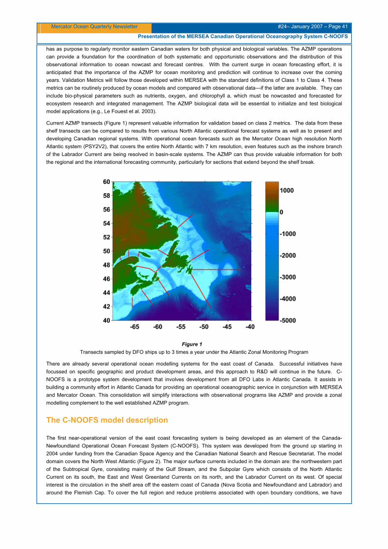
This month’s newsletter is dedicated to Operational Oceanography around the world, with a focus on the European MERSEA (http://www.mersea.eu.org/), the international GODAE (http://www.bom.gov.au/bmrc/ocean/GODAE/) programs as well as the GMES (see Figure) (http://www.gmes.info/) initiative. Mercator Ocean is already fully involved in MERSEA as well as in GODAE and GMES and will be one of the main actors of the Marine Core Service within the GMES project.
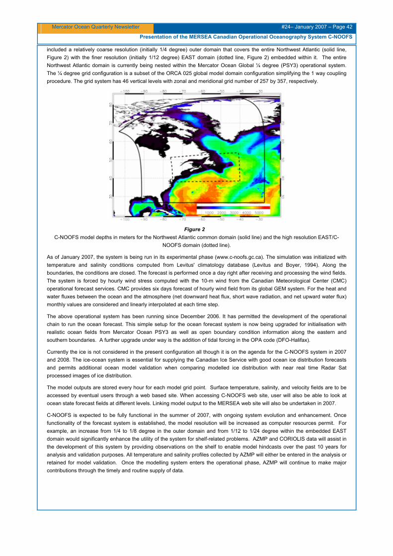
After an introduction by Desaubies reminding us of the challenges of the MERSEA project, this issue displays four articles giving us a broad overview of what is done in the world of operational oceanography. We first start with an article illustrating how the Mercator Ocean GMES Marine Core services are useful to downstream services such as Ocean climate monitoring, seasonal prediction and support to offshore industry. We then follow with an article by our Australian colleagues (Brassington et al.) involved in GODAE, describing their BlueLink operational oceanography system. Next article (Crosnier et al.) show how we collaborate at the international GODAE level in order to inter-compare the forecasting systems, with an example of comparison of the Mercator Ocean and BlueLink systems in the Indian Ocean. And last but not least article is written by our Canadian colleagues (Davidson et al.) involved in the MERSEA and GODAE projects, describing their Canadian Ocean Forecasting System. We wish you a pleasant reading and will meet again in April 2007, with a newsletter dedicated to impact studies.
News : MERSEA - development of GMES Marine Core Services. ..................................................................... 3
Within the GMES and towards the Marine Core Service at Mercator Ocean.................................................... 6
BLUElink> delivers first ocean forecasts .......................................................................................................... 20
GODAE at work in the Indian Ocean and Australian area: metrics definition and intercomparison of the BLUElink and Mercator systems........................................................................................................................ 31
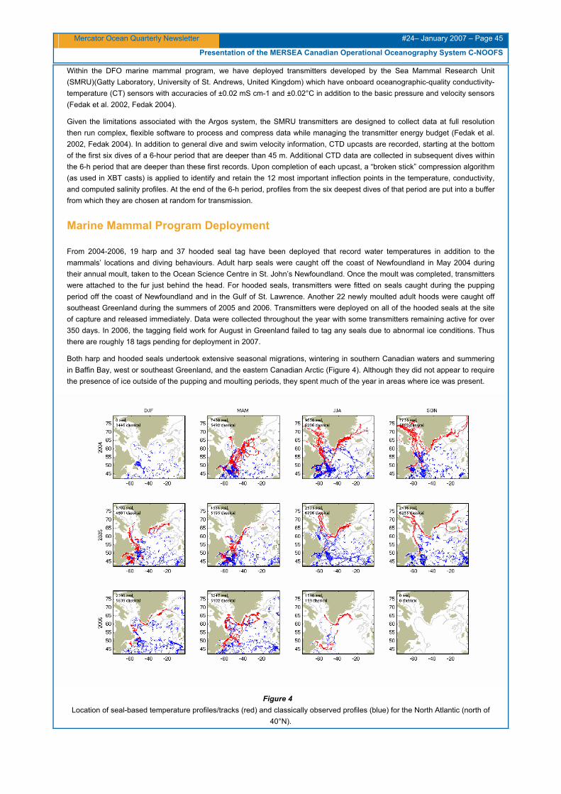
Presentation of the MERSEA Canadian operational oceanography system C-NOOFS.............................................................................................................................................................. 40
News: Mersea – Development of GMES Marine Core Services
News: Mersea - Development of GMES Marine Core Services. By Yves Desaubies
IFREMER – BP 70. 29280 Plouzané
The Mersea project, funded since 2004 by the European Commission to develop ocean and marine applications for GMES1, will soon enter its fourth and final year. By its end in March 2008, the project will deliver an integrated system for ocean monitoring and forecasting, which will serve as the basis of the Marine Core Services for GMES.
The Mersea system is based on the assimilation of remote sensing (altimetry, sea surface temperature, sea ice, ocean colour) and in situ observations (Argo and XBT profiles) into high resolution ocean models.
As a research and development project, Mersea is structured on twelve work packages covering four broad categories of activities: scientific research, architecture and design of the system, operation and production, development of applications and engaging stakeholders.
Research
The research plan is tackling a wide range of problems of direct relevance to the improvement and validation of the systems.
Validated, merged satellite data products and long time series are elaborated from different sensors: for altimetry, a fifteen year re-analysis with daily resolution is prepared, a new dynamic topography is being derived, and specific regional products are elaborated; sea surface temperature focuses on high resolution products for the global ocean and the Mediterranean; processing of ocean colour data for diffuse attenuation coefficient, surface chlorophyll and primary production, here again with long term re-analysis and regional products; sea ice fields to obtain velocity and thickness in the both hemispheres.
Work on forcing fields is concerned with merged wind products from combined satellite and numerical weather prediction; improved flux parameterisation from bulk formulae is also derived.
Ocean modelling and data assimilation are at the core of the monitoring and forecasting systems. Significant efforts are devoted to research on physical modelling (towards a global version, 1/12°, version of the NEMO code, with partial steps, prognostic sea-ice, improved mixed layer, tidal mixing), techniques for downscaling and nesting of models, and different advanced schemes for assimilation (Ensemble Kalman, SIR, and SEEK filters).
Ecosystem and bio-geochemical modelling is an area of active research and fast progress; the objective of the project is to include primary ecosystem in the monitoring and forecasting systems. The approach is somewhat different for the global ocean and for the regional seas. For the global ocean, one approach is the investigation of the so-called “class-size spectral” approach, appropriate to describe the cycling of nitrogen and carbon in the upper ocean with a minimum number of explicit variables and difficult-to-constrain parameters. Structural elements of this new model are the flows of energy and nutrients through phyto- and zoo plankton of different size, governed by an implicit representation of the size spectrum.
Alternatively, models of the NPZD type are pursued for integration into OPA (LOBSTER and PISCES) together with improved assimilation schemes (for physical and biochemical variables).
At another extreme in the level of complexity, ecosystems of the functional group type are experimented with in the North-West shelf environment and the Mediterranean sea. Those models attempt to resolve different species or groups of plankton, and may typically include several dozens of variables. For example the European Regional Seas Ecosystem Model (ERSEM) for the North-West shelves or the Biogeochemical Flux Model (BFM) for the Mediterranean.
Realistic modelling of ecosystems and global bio-geochemistry is a considerable challenge that places stringent requirements on the physical as well as the biological models. It is a very active area of research where further progress is expected in the coming years. The potential impact on monitoring of the carbon cycle and primary production is of high relevance to societal concern for sustainable development.
Seasonal forecasting is another area where the potential benefits of high resolution ocean state description are investigated (see the 2nd article, part2 by Ferry et al.).
1 Global Monitoring for Environment and Security: a European initiative for the implementation of information services dealing with environment and security; it will mainly support decision-making by both institutional and private actors.
News: Mersea – Development of GMES Marine Core Services
Architecture and design
The design is based on an integrated network of dedicated thematic centres: three Thematic Assembly Centres (TAC) for the input data (Earth Observations from satellites, in situ oceanographic data, and surface fluxes at the ocean-atmosphere interface), and five modelling/assimilation Monitoring and Forecasting Centres (MFC) linked to the geographical coverage of the forecasts (Global ocean, and regional seas of Europe: Arctic and Nordic seas, North and Baltic seas, North West shelves, and Mediterranean). The Centres are integrated through an Information Management System. A common approach is followed on data formats, procedures, protocols and services. The system based on those thematic centres is designed to optimise resources, to avoid duplication and to implement true European integration. It provides a coherent, efficient and sustainable shared information system for GMES ocean services.
The Target Operational Period
An initial version of the Mersea system has been running since July 2004; several upgrades of the system have been implemented in October 2005, at the start of the first target operational period, which ran for six months and is continuing. All the systems are producing daily (or weekly for the global) analyses and forecasts. The next upgrades will be in April 2007, at which time the second 6-month Target Operational Period (TOP2) will start, for which four major objectives have been set:
Objective 1: Implement version V2 of the system with assessments and validation. The different versions of the system are described in the overall work plan. At this stage, the most significant upgrades include transition of some of the systems to the NEMO code, higher resolution, process parameterisation, ice modelling, nesting, and multivariate data assimilation.
Assessment and validation will be based on the Class 1 to 3 metrics that were used in the Mersea Strand 1 project and on Class 4 (see article 4 by Crosnier et al.).
Objective 2: provide a clear visibility of the Mersea system in operation and of its products. This will include improvements in the viewing, discovery and downloading services; a wider set of Mersea standard products and catalogue will be elaborated. Ocean indicators will be calculated, produced and displayed. Indicators must be carefully defined in order to be appropriate for specific purposes. In general, indicators are meant to summarize complex data sets in a simple way. Thus they can be useful data sets for scientific interpretation –in which case great care must be taken to give proper interpretation and full validation (or error bars); or for ocean monitoring and reporting in the framework of Conventions –in which case they must be relevant to a particular policy objective; or they could simply serve as illustration of the output of the Mersea system for a general public.
Improved visibility of the Mersea system will also involve a revision of the web site and its displays.
Objective 3: is to demonstrate the links with public institutions. This is admittedly a longer term objective that will require continuous interaction with the relevant agencies. During the last year several significant contacts have been made with the European Environmental Agency (EEA) and ICES. In particular, a joint workshop EuroGOOS, MERSEA and EMMA (European Marine Monitoring and Assessment) was held in Copenhaguen in October 2006, which opened the way for further convergence on environmental reporting.
Objective 4: demonstrate links with end-users. One such example is the support to offshore oil operations (see the 2nd article, part3 by Giraud et al.). Other applications are being considered: e.g. wave, currents and sea ice forecasts in support of ship-routing.
Marine Core Services
Multiple uses of the seas pose multiple challenges; they require different types of data, products and information and delivery system; over a wide range of scales, from global to the very local. But they share common requirements (observing systems, monitoring, forecasting), and need a coherent understanding of the ocean environment. The Marine Core Services (MCS) are developed as one of the components of the GMES system; they constitute the common foundation upon which specific products can be developed.
The Mersea project has worked very closely with the GMES Project Office (and its Implementation Panel) in defining the MCS, and only some of the key considerations can be summarized here. The main purpose of the MCS is to make available a set of basic, generic services based upon baseline ocean state variables required to meet the needs for information of those responsible for environmental and civil security policy making, assessment and implementation.
The services are meant to extend beyond production, access and delivery, to include also support in the form of assessment and expertise, research and development, training and user support.
News: Mersea – Development of GMES Marine Core Services
The MCS are aimed at intermediate users, i.e. agencies, companies, laboratories or individuals who will use the generic information to develop scientific applications or specific products aimed at end-users. A prime category of intermediate users are the coastal or national systems involved in near-shore management or agencies (e.g. met agencies) in charge of support for marine safety, search and rescue operations, etc… Similarly, scientists involved in ICES need synthetic ocean information to produce their reports. There are also strong policy drivers for the MCS, in particular the Regional Conventions (e.g. OSPAR, HELCOM) and the recently adopted European Marine Strategy Directive.
It is the intention of the European Commission to foster the transition of MCS from a research context towards a fully operational system, with stringent requirements on reliability, robustness, standards, service level agreements, etc… Funding towards that objective is identified in the FP7, as one of the mature Fast Track Services.
Perspectives
The Mersea project is funded to develop “Ocean and Marine Applications for GMES”. In the course of the project this has progressively evolved towards the definition of the MCS, with significant progress in their initial implementation.
Thus the Mersea project, building on previous efforts by many scientists and agencies, will contribute significantly to the establishment of permanent ocean monitoring and forecasting systems.
Among the many challenges to solve in the future one can mention the full validation of the systems, approaches to multi model or ensemble forecasts, further progress on ecosystem modelling, strengthened links with coastal systems, development of user applications, and outreach to users outside Europe.
Other aspects to be solved in the future include funding, institutional framework, and data policy.
In its final year the Mersea must achieve its goals, as set forth in its work plan, which will mark a significant step on the road to permanent operational marine services in Europe.
Acknowledgment
This work is a contribution to the MERSEA project. Partial support of the European Commission under contract SIP3-CT-2003-502885 is gratefully acknowledged. (http://www.mersea.eu.org)
Mercator Ocean Quarterly Newsletter #24– January 2007 – Page 6
Within the GMES and towards the Marine Core Service at Mercator Ocean
Within the GMES and towards the Marine Core Service at Mercator Ocean By (in alphabetical order): Laurence Crosnier1, Marie Drévillon2, Nicolas Ferry1, Sylvie Giraud3, S. Gualdi4, Jean -François Guérémy5, Fabrice Hernandez1, David Kempa1, Véronique Landes1, Didier Palin1, Elisabeth Rémy2, Alberto Troccoli6, Antony Weaver2 1 Mercator Ocean – 8/10 rue Hermès. 31520 Ramonville st Agne 2 CERFACS – 42 avenue Gaspard Coriolis. 31100 Toulouse 3 CLS – 8/10 rue Hermès. 31520 Ramonville st Agne 4 INGV – Via Donato Creti 12. 40128 Bologna (Italie) 5 Météo France – 42 avenue Gaspard Coriolis. 31100 Toulouse 6 ECMWF – Shinfield Park. Reading RG2 9AX (UK)
Introduction
The GMES (Global Monitoring for Environment and Security) (http://www.gmes.info/) is a European initiative jointly supported by the European Commission and the European Space Agency (ESA), for the implementation of information services dealing with environment and security. Mercator Ocean is already involved in the GMES through the MERSEA (http://www.mersea.eu.org/), MARCOAST/ROSES (http://marcoast.info/) and BOSS4GMES (http://www.boss4gmes.eu) projects. Mercator Ocean is also currently coordinating the European partners for the preparation and submission of the proposal answering the Seventh Framework Programme (FP7) European Union call in order to further build the GMES services.
GMES services are classified in three major categories:
1- Mapping of - topography, road, land-use, harvest, forestry, mineral and water resources- that contribute to short and long-term management of territories and natural resources.
2- Support for emergency management in case of natural hazards as well as support for civil institutions responsible for the security of people and property.
3- Forecasting is applied for marine zones, air quality or crop yields. This service includes the Marine Core Service (MCS) which goal is to forecast, monitor and report on the ocean state for both the global ocean and the regional European seas. Mercator Ocean will mainly intervene in this category. The MCS is, as its name indicates, the Core service providing information to Downstream services which goals are:
1. To better exploit and manage ocean resources (e.g. offshore oil and gas industry, fisheries)
2. Seasonal climate prediction
3. Implement specific services for coastal management and planning (e.g. coastal flooding and erosion)
4. Marine research (e.g. better understanding of the oceans and their ecosystems, of ocean climate variability)
5. Improve safety and efficiency of maritime transport, shipping, and naval operations
6. Anticipate and mitigate the effects of environmental hazards and pollution crisis (e.g. oil spills, harmful algal blooms)
This paper splits into 3 parts which all illustrate how the Mercator Ocean Marine Core services are used for Downstream services listed above. The first part introduces ocean climate indices to monitor climate variability. The second part is dedicated to the work on seasonal prediction going on within the MERSEA project. The last part deals with the Mercator Ocean/CLS ocean services in the Gulf of Mexico which are delivered by the intermediate users’ company Ocean Numerics and provided to private oil companies.
Mercator Ocean Quarterly Newsletter #24– January 2007 – Page 7
Within the GMES and towards the Marine Core Service at Mercator Ocean
Part1: Ocean indices for climate monitoring of the global ocean By: Laurence.Crosnier (Mercator Ocean), Marie Drévillon (CERFACS), Elisabeth Rémy (CERFACS), Fabrice Hernandez (Mercator Ocean)
Ocean climate indices provide information for a better understanding of the oceans and their ecosystems, as well a simple representation of ocean climate variability. They also allow, in the best case scenario, to anticipate the effects of environmental hazards and pollution crisis. Ocean climate indices are linked to major patterns of climate variability with significant social, economical and environmental impact. They provide an at-a-glance overview of the state of the ocean climate, and a way to talk to a wider audience about the ocean observing system.
Mercator Ocean is currently working on defining pertinent Ocean Climate Indices using the various Mercator Ocean operational models and also using observational analyses sourced from different operational centers. Such indices are updated on a weekly or monthly basis. Two examples as well as their relevance are given here.
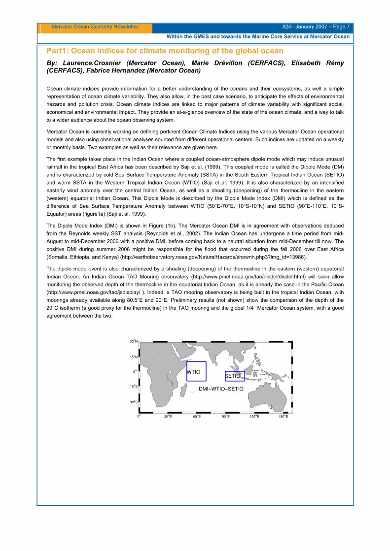
The first example takes place in the Indian Ocean where a coupled ocean-atmosphere dipole mode which may induce unusual rainfall in the tropical East Africa has been described by Saji et al. (1999). This coupled mode is called the Dipole Mode (DM) and is characterized by cold Sea Surface Temperature Anomaly (SSTA) in the South Eastern Tropical Indian Ocean (SETIO) and warm SSTA in the Western Tropical Indian Ocean (WTIO) (Saji et al. 1999). It is also characterized by an intensified easterly wind anomaly over the central Indian Ocean, as well as a shoaling (deepening) of the thermocline in the eastern (western) equatorial Indian Ocean. This Dipole Mode is described by the Dipole Mode Index (DMI) which is defined as the difference of Sea Surface Temperature Anomaly between WTIO (50°E-70°E, 10°S-10°N) and SETIO (90°E-110°E, 10°S-Equator) areas (figure1a) (Saji et al. 1999).
The Dipole Mode Index (DMI) is shown in Figure (1b). The Mercator Ocean DMI is in agreement with observations deduced from the Reynolds weekly SST analysis (Reynolds et al., 2002). The Indian Ocean has undergone a time period from mid-August to mid-December 2006 with a positive DMI, before coming back to a neutral situation from mid-December till now. The positive DMI during summer 2006 might be responsible for the flood that occurred during the fall 2006 over East Africa (Somalia, Ethiopia, and Kenya) (http://earthobservatory.nasa.gov/NaturalHazards/shownh.php3?img_id=13986).
The dipole mode event is also characterized by a shoaling (deepening) of the thermocline in the eastern (western) equatorial Indian Ocean. An Indian Ocean TAO Mooring observatory (http://www.pmel.noaa.gov/tao/disdel/disdel.html) will soon allow monitoring the observed depth of the thermocline in the equatorial Indian Ocean, as it is already the case in the Pacific Ocean (http://www.pmel.noaa.gov/tao/jsdisplay/ ). Indeed, a TAO mooring observatory is being built in the tropical Indian Ocean, with moorings already available along 80.5°E and 90°E. Preliminary results (not shown) show the comparison of the depth of the 20°C isotherm (a good proxy for the thermocline) in the TAO mooring and the global 1/4° Mercator Ocean system, with a good agreement between the two.
Mercator Ocean Quarterly Newsletter #24– January 2007 – Page 8
Within the GMES and towards the Marine Core Service at Mercator Ocean
Figure1
a) location of WTIO and SETIO boxes in the Indian Ocean (Saji et al. 1999) b) Dipole Mode Index: difference of SSTA in WTIO and SETIO boxes in the global 1/4° Mercator Ocean system (black line)
and in Reynolds OI-v2 weekly SST analysis (Reynolds et al. 2002) (red line). The Mercator Ocean SST Anomaly is computed relative to a 10year (1992-2001) free run without data assimilation. The Reynolds SST Anomaly is computed relative to the
Reynolds 1971-2000 climatology (Reynolds et al. 2002).
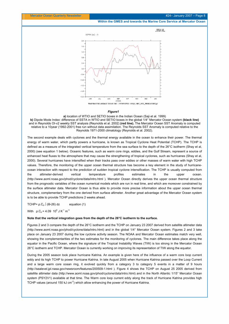
The second example deals with cyclones and the thermal energy available in the ocean to enhance their power. The thermal energy of warm water, which partly powers a hurricane, is known as Tropical Cyclone Heat Potential (TCHP). The TCHP is defined as a measure of the integrated vertical temperature from the sea surface to the depth of the 26°C isotherm (Shay et al, 2000) (see equation 1 below). Oceanic features, such as warm core rings, eddies, and the Gulf Stream, represent a source of enhanced heat fluxes to the atmosphere that may cause the strengthening of tropical cyclones, such as hurricanes (Shay et al, 2000). Several hurricanes have intensified when their tracks pass over eddies or other masses of warm water with high TCHP values. Therefore, the monitoring of the upper ocean thermal structure has become a key element in the study of hurricane-ocean interaction with respect to the prediction of sudden tropical cyclone intensification. The TCHP is usually computed from the altimeter-derived vertical temperature profiles estimates in the upper ocean. (http://www.aoml.noaa.gov/phod/cyclone/data/intro.html ). Mercator Ocean directly derives the upper ocean thermal structure from the prognostic variables of the ocean numerical models which are run in real time, and which are moreover constrained by the surface altimeter data. Mercator Ocean is thus able to provide more precise information about the upper ocean thermal structure, complementary from the one derived from surface altimeter. Another great advantage of the Mercator Ocean system is to be able to provide TCHP predictions 2 weeks ahead.
TCHP= ρ.Cp ∫ (Ө-26) dz equation (1)
With ρ.Cp = 4.09 106 J K-1 m-3
Note that the vertical integration goes from the depth of the 26°C isotherm to the surface.
Figures 2 and 3 compare the depth of the 26°C isotherm and the TCHP on January 23 2007 derived from satellite altimeter data (http://www.aoml.noaa.gov/phod/cyclone/data/intro.html) and in the global 1/4° Mercator Ocean system. Figures 2 and 3 take place on January 23 2007 during the low cyclone activity season. The NOAA and Mercator Ocean estimates match very well, showing the complementarities of the two estimates for the monitoring of cyclones. The main difference takes place along the equator in the Pacific Ocean, where the signature of the Tropical Instability Waves (TIW) is too strong in the Mercator Ocean 26°C isotherm and TCHP. Mercator Ocean is currently working on improving its representation of TIW along the equator.
During the 2005 season took place hurricane Katrina. An example is given here of the influence of a warm core loop current eddy and its high TCHP to power Hurricane Katrina. In late August 2005 when Hurricane Katrina passed over the Loop Current and a large warm core ocean ring, it evolved quickly from a category 3 to category 5 events in a matter of 9 hours (http://sealevel.jpl.nasa.gov/newsroom/features/200509-1.html ). Figure 4 shows the TCHP on August 25 2005 derived from satellite altimeter data (http://www.aoml.noaa.gov/phod/cyclone/data/intro.html) and in the North Atlantic 1/15° Mercator Ocean system (PSY2V1) available at that time. The Warm core loop current eddy along the track of Hurricane Katrina provides high TCHP values (around 150 kJ cm-2) which allow enhancing the power of Hurricane Katrina.
Mercator Ocean Quarterly Newsletter #24– January 2007 – Page 10
Within the GMES and towards the Marine Core Service at Mercator Ocean
Figure4
Tropical Cyclone Heat Potential (kJ cm-2) (TCHP) on August 25 2005 (Top) derived from satellite altimeter data (http://www.aoml.noaa.gov/phod/cyclone/data/intro.html) (middle) in the North Atlantic 1/15° Mercator Ocean system (PSY2V1). (bottom) Sea height anomaly on August 28, 2005. The path of Hurricane Katrina is indicated with circles spaced every 3 hours
in the Gulf of Mexico and their size and color represent intensity (see legend). The hurricane intensified to category 5 as it passed near the warm core eddy of the Loop Current, then diminished to category 4 by the time it struck the coast. From
The two examples of ocean indices shown here are part of a larger work still going on at Mercator Ocean within the GMES framework. Mercator Ocean is currently working on publishing on its website several ocean indices updated on a weekly or monthly basis. The aim is to talk to a wider audience and to provide a simple representation of ocean climate variability.
Seasonal forecasting (or seasonal prediction) consists in predicting several months in advance climate parameters like the 2 metre air temperature or precipitation on a large spatial scale, typically on a regional scale like southern Europe, and averaged over a season. It is not a question of producing a detailed weather forecast like the one broadcasted daily by national weather centres, in which the temperature and the precipitation at a certain location are predicted for a few days in advance. Rather, one seeks to determine the “average” weather (or climate) conditions that will occur several months ahead. For this, one uses a probabilistic approach which indicates a level of probability of having a type of climate close to or far from the seasonal norm (for example, if the climate will be warmer or rainier than normal, etc.). Thus, the seasonal forecast carried out in February will make it possible to determine for example the type of weather that there will be in Western Europe for the beginning of the next summer.
State-of-the-art seasonal forecasting is carried out by coupling global oceanic and atmospheric general circulation models (GCMs). These models generally have coarse spatial resolution because they are integrated over long periods (several months for individual forecasts) with various initial conditions. Moreover, to calibrate the coupled model forecasts, past integrations or hindcasts must be performed over extensive periods (several years). To fix the ideas, Météo-France which produces seasonal forecasts uses the ARPEGE-Climat atmospheric model with truncation T63L31 (~2.8° horizontal resolution) coupled with the OPA-ORCA2 oceanic model (~2° horizontal resolution). As the oceanic structure varies much slowlier than that of the atmosphere, a part of the atmospheric predictability comes from the initial state of the ocean. For example, certain oceanic conditions can support the development of an anticyclonic blocking activity over Europe or alternatively support an important cyclogenesis. One of the challenges of seasonal climate prediction is thus to correctly initialise the ocean model, which contains to some extent the memory of the climate machine (the ocean and the atmosphere). It is on this particular aspect of the ocean state initialisation that Mercator Ocean contributes by performing oceanic reanalysis with data assimilation and by delivering oceanic initial conditions (ICs) to numerical weather prediction (NWP) centres for seasonal forecasts. Finally, it should be emphasized that as seasonal forecasts are probabilistic, forecast-producing centres are not satisfied with just one (deterministic) climate forecast but require several forecasts (in general a few tens) in order to sample both the chaotic nature of the climate system and errors in the climate-prediction model. Here, one seeks to sample which will be the most probable state of the atmosphere in the future.
Lessons learnt from the MERSEA project
The European Community funded MERSEA Integrated Project aims at setting up, by 2008, a European capacity of monitoring and forecasting the ocean on global and regional scales, in the fields of physics, bio-geochemistry and oceanic ecosystems. Several demonstrations of applications are developed in this project, one of which is the contribution to the improvement of the seasonal forecasts and the observation of climatic variability. It is within this framework that the European Centre for Medium-Range Weather Forecasts (ECMWF), Mercator Ocean, Météo-France (France) and Instituto Nazionale di Geofisica e Vulcanologia (INGV, Italy) set up a common research and development programme. Its objectives are to test new ways to initialise ocean models used for coupled seasonal forecasts. This programme (called Special Focus Experiments or SFE) aims in particular at taking advantage of global ocean analyses at high resolution (1/4°) developed within the framework of the MERSEA project (see http://w3.mersea.eu.org/html/ocean_modelling/global_tep.html) by using them as initial conditions for coupled seasonal forecasts. The idea is that these analyses at high resolution should be closer to reality than oceanic analyses obtained with a coarser resolution model, which is generally the case. The same issue concerns atmospheric GCMs where the resolution is potentially a limiting factor. Increasing the horizontal resolution of the atmospheric component of the coupled model is also a possibility for improving the coupled seasonal prediction model.
This SFE is addressing the following questions. What is the optimal resolution for the atmospheric and oceanic GCMs in order to have the best seasonal prediction skill? Is it possible to increase the predictability by initialising the ocean model with ICs provided by a high resolution ocean GCM like the MERSEA-1/4° analyses? Figure 1 summarizes the strategy adopted to answer these questions. Mercator Ocean has performed extensive sets of ocean simulations specially tuned for seasonal prediction purposes at 2° and ¼° spatial resolution. These ocean ICs are then used in various model configurations by ECMWF, Météo-France and INGV to perform seasonal forecasts with the objective to provide answers to the questions above. The use of multiple atmospheric GCMs (IFS by ECMWF, ARPEGE-Climat by Météo-France and ECHAM by INGV) is one of the important aspects of the SFE.
Mercator Ocean Quarterly Newsletter #24– January 2007 – Page 12
Within the GMES and towards the Marine Core Service at Mercator Ocean
Figure 1 Schematic view of the method used to determine the optimal seasonal forecast strategy according to the resolution of the ocean
analyses and / or ocean / atmosphere GCMs used.
Strategy A is the classical approach used at ECMWF or Météo-France for seasonal forecasts: Two global coarse resolution oceanic and atmospheric GCMs are coupled and the ocean model is initialised with an ocean IC obtained with a coarse resolution ocean analysis (2°). The advantage of this methodology is that seasonal forecasts can be done with numerous members.
Stragtegy B is the same as strategy A except that the ocean IC comes from a high resolution ocean model analysis (1/4°) appropriately interpolated on the coarse ocean model grid. This approach tests the impact of high resolution ocean analysis as ICs for coarse resolution ocean models coupled with an atmospheric GCM.
Strategy C consists of coupling two global high resolution oceanic and atmospheric GCMs and initialising the ocean IC with a high resolution ocean analysis (1/4°). This approach is potentially highly efficient but computationally very expensive. For this case, seasonal prediction can be done with only a few members.
For example, it is important to know if an atmospheric GCM coupled to an oceanic coarse resolution model initialised with a high resolution (1/4°) ocean analysis makes it possible to improve seasonal forecast skill (strategy A versus B). Or, is it better to carry out many simulations at coarse resolution (strategy A or B) or few simulations at high resolution (strategy C) to have the best seasonal forecast skill? It is these kinds of questions that are being investigated in the SFE. It should be noted that without the impetus of the European MERSEA project, this collaboration between ECMWF, Mercator Ocean, Météo-France and INGV would certainly not have been possible. The conclusions of this work in progress will provide the basis of what should be the future seasonal forecast system operated for the Global Monitoring for Environment and Security (GMES) service. This should finally help improving the European policies of energy stock management, agriculture, environment, etc… depending on climatic factors in the seasonal range (up to about six months).
Mercator Ocean Quarterly Newsletter #24– January 2007 – Page 13
Within the GMES and towards the Marine Core Service at Mercator Ocean
Seasonal forecasting activity as a downstream application of the Marine Core Service: how would it look like?
The Seventh Framework Programme for research and technological development (FP7) was adopted and first calls for proposals were published end of December 2006. One of them is of interest for GMES-related activities and in particular for seasonal forecasting purposes (Space Call 1 FP7-SPACE-2007-1, see http://www.gmes.info/newsdetail+M5fd64738f07.0.html).
This document indicates that “the objective of the Marine Core Service (MCS) is to improve EU capacities for monitoring and predicting the marine environment with an integrated capacity to provide data and information required by a range of downstream service providers relating to the global oceans (…). Nowcasts, forecasts and analyses covering a period of 20-50 years will be produced and used to monitor and understand the changes in the state of the ocean.”
The implications for Mercator Ocean are multiple.
First, Mercator Ocean operational activities of global ocean state analysis, used in particular within the framework of the MERSEA Special Focus Experiment, can be used for downstream seasonal forecasting applications. It is already the case for example for the Mercator Ocean system (PSY2Gv1) (Ferry, 2004) which provides initial conditions (IC) for coupled seasonal forecasts performed by Météo-France. These seasonal predictions also contribute to Euro-SIP (European Seasonal to Interannual Prediction project), a collaborative project between ECMWF, Météo-France and the UK Met Office to produce operational, real-time, multi-model global seasonal forecasts.
Second, advanced data assimilation schemes for operational analysis and forecasting of the ocean developed at Mercator Ocean for many years will contribute to a better estimation of the ocean state and accurate ICs for downstream services as seasonal forecasts. Indeed, in early 2007 the version2 MERSEA 1/4° global systems (PSY3V2) as well as the Mercator coarse resolution global system (~2°) (PSY2Gv2), will take advantage of a new multivariate analysis scheme based on a reduced-order Kalman filter (a variant of the SEEK filter developed at LEGI ,Grenoble) which assimilates altimetric, sea surface temperature and in situ data (profiles of temperature and salinity). Other advanced techniques based on 3D and 4D variational data assimilation are being investigated at Mercator in collaboration with CERFACS (Toulouse) and ECMWF. The cost-versus-benefits for seasonal prediction of reduced-order Kalman filtering and variational assimilation is an open question. In an ensemble forecasting system, however, these methods may be complementary by providing independently-derived ocean state estimates. This could be an effective and practical way of sampling uncertainty in ocean initial conditions. It is thus possible that the two methods could be used together to improve seasonal prediction skill. This ongoing effort will finally contribute to have the best possible estimate of the ocean state and accurate ICs for seasonal forecasts.
Reanalyses covering a period of 20 to 50 years are part of the Marine Core services. Mercator Ocean already has some experience in this domain by producing the MERA-11 reanalysis (Greiner et al. 2006), a 11 year-long reanalysis for the North Atlantic Ocean. The operational setting of Mercator Ocean’s next global coarse resolution oceanic analysis/forecast system PSY2Gv2 will also be accompanied by the delivery of a 25-year long reanalysis. This will be very useful for seasonal forecasting purposes. However, the challenge for the coming years is a project of global ocean reanalysis at mesoscale which will be carried out with the global ¼° model. The objective is to describe realistically the oceanic state during the last 50 years by taking into account all the available oceanic observations. This project is under development and will mobilize probably a large portion of the European scientific community, by also building on prior experience gained through other European projects such as the FP5 ENACT project (2002-2004).
Lastly, one can note that the quality of the oceanic analyses at high resolution carried out today suggests that coupling the atmosphere to an ocean model could improve the medium-range weather forecasts (typically from 1 to 14 days). This assumption will be tested in MERSEA SFE by coupling the MERSEA-¼ ° global model with the ECMWF high resolution medium range forecast model IFS. The idea is that the oceanic coupling could in certain cases (in particular for extreme weather phenomena) improve the predictability of the atmosphere. Providing oceanic ICs for downstream medium range weather forecasting could also be one of Mercator Ocean’s activities for the future Marine Core Service.
Mercator Ocean Quarterly Newsletter #24– January 2007 – Page 14
Within the GMES and towards the Marine Core Service at Mercator Ocean
Part3: Environmental Security for Offshore Operators : the Ocean Focus Service in the Gulf of Mexico by Sylvie Giraud (CLS) and the Mercator Ocean Team of Ocean forecasters, David Kempa (Mercator Ocean), Didier Palin (Mercator Ocean) and Véronique Landes (Mercator Ocean)
A nowcasting and forecasting service of the ocean environment
“Ocean Focus” is an innovative ocean circulation nowcasting and forecasting service for Oil and Gas industry provinces worldwide. The service is designed to provide reliable, practical, cost-effective ocean circulation information “on demand”, i.e. when and where needed to support offshore operations at sea.
“Ocean Focus” is a demonstration of the commercial applications of operational oceanography that is developed downstream Mercator Ocean and that is provided to the end-users by an intermediate users company “Ocean Numerics” which is a joint venture between CLS, NERSC, FuGro GEOS and Ocean Weather Inc. This group of people gathers strong thematic competences in the Met-Ocean domain that range from leading-edge oceanographic and atmospheric science (ocean modelling, data assimilation, earth observations data merging, ocean forecasters), goes to operational system development and exploitation until reaching the commercial aspects with direct contact with major offshore companies at highest rank. They know precisely the offshore end-users needs.
Mercator Ocean joined this collaborative effort in order to assess (in delayed mode) and demonstrate (in real time) the value of its ocean products in the Gulf of Mexico region where the trials took place. It was a good opportunity to start addressing the question of the usability of the “GODAE-standards” ocean products for downstream applications, i.e. are the existing products good enough for end-users from the offshore industry and how can we improve them if ever ?
The final goal of this collaboration was to build an operational Real-time service based on Earth Observations data and on a multi-model analysis (TOPAZ, Mercator Ocean). This was achieved in 2006 when the intermediate user Ocean Numerics contracted with Mercator Ocean for model outputs. The clients of Ocean Numerics were BP & SHELL (from Feb. to July 2006), Exxon & Chevron (forecast evaluation until end of Aug. 2006).
The motivation of the service: facing tough ocean conditions
This service was designed for offshore oil and gas operators to help them facing their duties regarding the safety of the persons and facilities and the protection of the marine environment when conducting practical operations at sea. Offshore activities are indeed performed in “extreme (environmental) conditions” caused by strong ocean currents that primarily influence the operations at the sea surface as well as in the deep Ocean. The need for reliable and accurate forecast information to support operational decision-making is crucial in the real-time as well as in the delayed mode (e.g. long-term time series for design criteria and operability analyses).
In the Gulf of Mexico region where the study took place, strong surface currents are related to the Loop Current pathway and its interaction with associated eddies. They can persist over several weeks. Maximum observed speed can reach 2 m/s in the Loop Current and its vertical shear extends down to 1000 m below the surface.
We make a special focus on the deepwater lease blocks across the northern Gulf that is the region directly impacted by the northern extension of the Loop Current and that shows high concentration of (deep) offshore platforms. It is also the place where the episodic detachment of a ring (or Loop Current Eddy) occurs before it starts migrating westwards along the Latex shelf. Last but not least, the Gulf is a region where the risks associated to the sea state are seasonally magnified by the “extreme events” known as the tropical storms and hurricanes like Katrina that caused dramatic damages to people and facilities in 2005. These ocean-atmosphere coupled events are beyond the scope of this article.
Adding Value to the core ocean products
Scientific Assessment of the value of the model ocean products: for a specific event Mercator Ocean “delayed mode” ocean products were scrutinized for the wintertime period in 2005 (before Katrina) and this work was documented in the Mercator Ocean Newsletter # 19 edited in October 2005.
The analysis stepped on three major items and focused on the “high-priority” event of interest for the end-user, that is the variability of the Loop Current front and the related Loop Current Eddy shedding event:
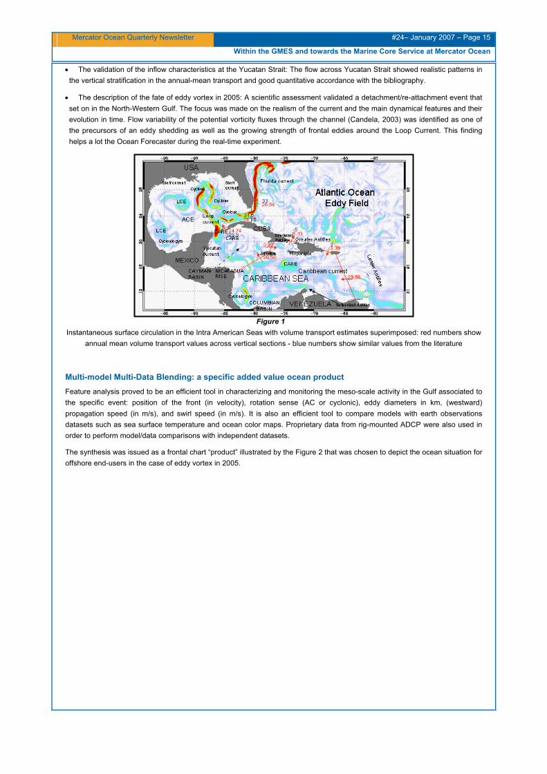
• The validation of the surface circulation in the Intra-American Seas, as shown by Figure 1.
Mercator Ocean Quarterly Newsletter #24– January 2007 – Page 15
Within the GMES and towards the Marine Core Service at Mercator Ocean
• The validation of the inflow characteristics at the Yucatan Strait: The flow across Yucatan Strait showed realistic patterns in the vertical stratification in the annual-mean transport and good quantitative accordance with the bibliography.
• The description of the fate of eddy vortex in 2005: A scientific assessment validated a detachment/re-attachment event that set on in the North-Western Gulf. The focus was made on the realism of the current and the main dynamical features and their evolution in time. Flow variability of the potential vorticity fluxes through the channel (Candela, 2003) was identified as one of the precursors of an eddy shedding as well as the growing strength of frontal eddies around the Loop Current. This finding helps a lot the Ocean Forecaster during the real-time experiment.
Figure 1
Instantaneous surface circulation in the Intra American Seas with volume transport estimates superimposed: red numbers show annual mean volume transport values across vertical sections - blue numbers show similar values from the literature
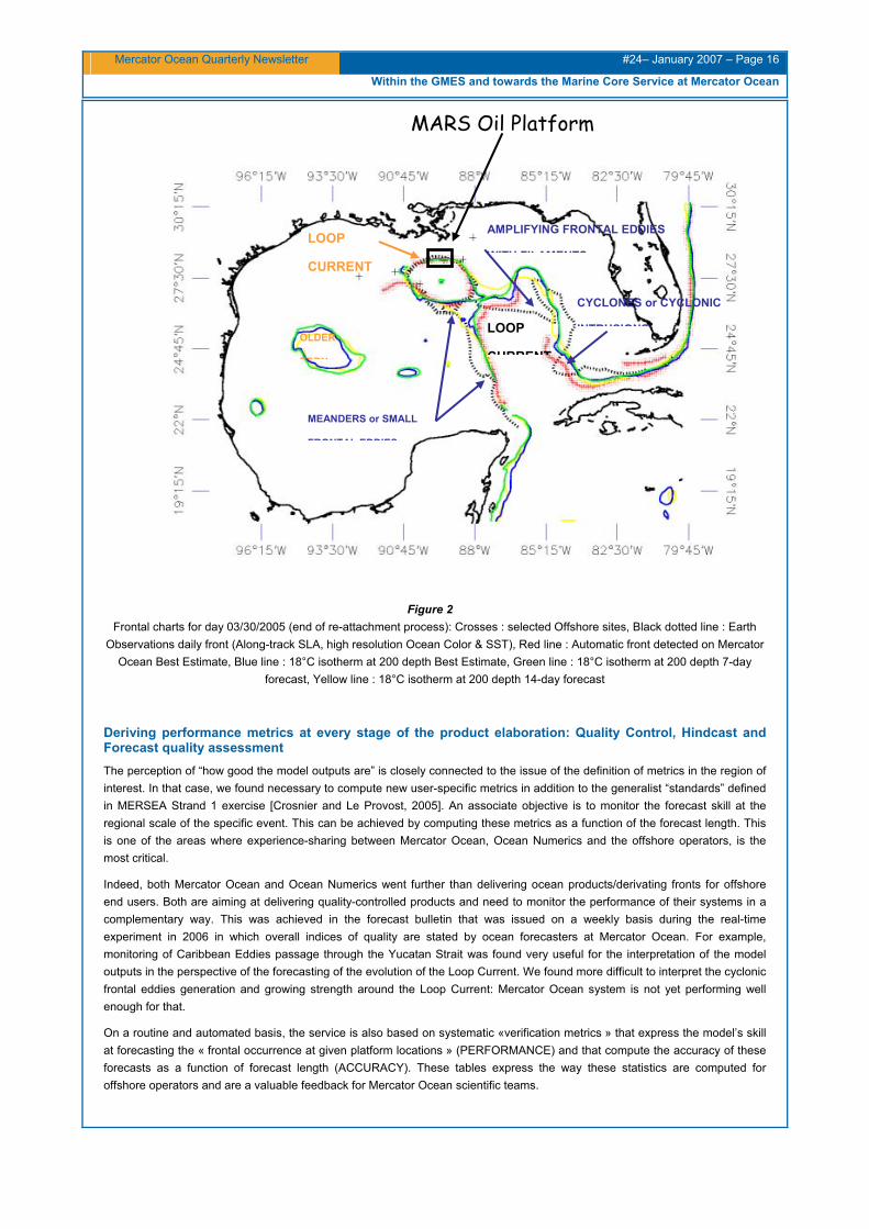
Multi-model Multi-Data Blending: a specific added value ocean product Feature analysis proved to be an efficient tool in characterizing and monitoring the meso-scale activity in the Gulf associated to the specific event: position of the front (in velocity), rotation sense (AC or cyclonic), eddy diameters in km, (westward) propagation speed (in m/s), and swirl speed (in m/s). It is also an efficient tool to compare models with earth observations datasets such as sea surface temperature and ocean color maps. Proprietary data from rig-mounted ADCP were also used in order to perform model/data comparisons with independent datasets.
The synthesis was issued as a frontal chart “product” illustrated by the Figure 2 that was chosen to depict the ocean situation for offshore end-users in the case of eddy vortex in 2005.
Mercator Ocean Quarterly Newsletter #24– January 2007 – Page 16
Within the GMES and towards the Marine Core Service at Mercator Ocean
AMPLIFYING FRONTAL EDDIES LOOP
WITH FILAMENTSCURRENT
CYCLONES or CYCLONIC
LOOP INTRUSIONSOLDER
CURRENTEDDY
MEANDERS or SMALL
FRONTAL EDDIES
Figure 2 Frontal charts for day 03/30/2005 (end of re-attachment process): Crosses : selected Offshore sites, Black dotted line : Earth
Observations daily front (Along-track SLA, high resolution Ocean Color & SST), Red line : Automatic front detected on Mercator Ocean Best Estimate, Blue line : 18°C isotherm at 200 depth Best Estimate, Green line : 18°C isotherm at 200 depth 7-day
forecast, Yellow line : 18°C isotherm at 200 depth 14-day forecast
Deriving performance metrics at every stage of the product elaboration: Quality Control, Hindcast and Forecast quality assessment The perception of “how good the model outputs are” is closely connected to the issue of the definition of metrics in the region of interest. In that case, we found necessary to compute new user-specific metrics in addition to the generalist “standards” defined in MERSEA Strand 1 exercise [Crosnier and Le Provost, 2005]. An associate objective is to monitor the forecast skill at the regional scale of the specific event. This can be achieved by computing these metrics as a function of the forecast length. This is one of the areas where experience-sharing between Mercator Ocean, Ocean Numerics and the offshore operators, is the most critical.
Indeed, both Mercator Ocean and Ocean Numerics went further than delivering ocean products/derivating fronts for offshore end users. Both are aiming at delivering quality-controlled products and need to monitor the performance of their systems in a complementary way. This was achieved in the forecast bulletin that was issued on a weekly basis during the real-time experiment in 2006 in which overall indices of quality are stated by ocean forecasters at Mercator Ocean. For example, monitoring of Caribbean Eddies passage through the Yucatan Strait was found very useful for the interpretation of the model outputs in the perspective of the forecasting of the evolution of the Loop Current. We found more difficult to interpret the cyclonic frontal eddies generation and growing strength around the Loop Current: Mercator Ocean system is not yet performing well enough for that.
On a routine and automated basis, the service is also based on systematic «verification metrics » that express the model’s skill at forecasting the « frontal occurrence at given platform locations » (PERFORMANCE) and that compute the accuracy of these forecasts as a function of forecast length (ACCURACY). These tables express the way these statistics are computed for offshore operators and are a valuable feedback for Mercator Ocean scientific teams.
MARS Oil Platform
Mercator Ocean Quarterly Newsletter #24– January 2007 – Page 17
Within the GMES and towards the Marine Core Service at Mercator Ocean
We compute three “user-specific” metrics:
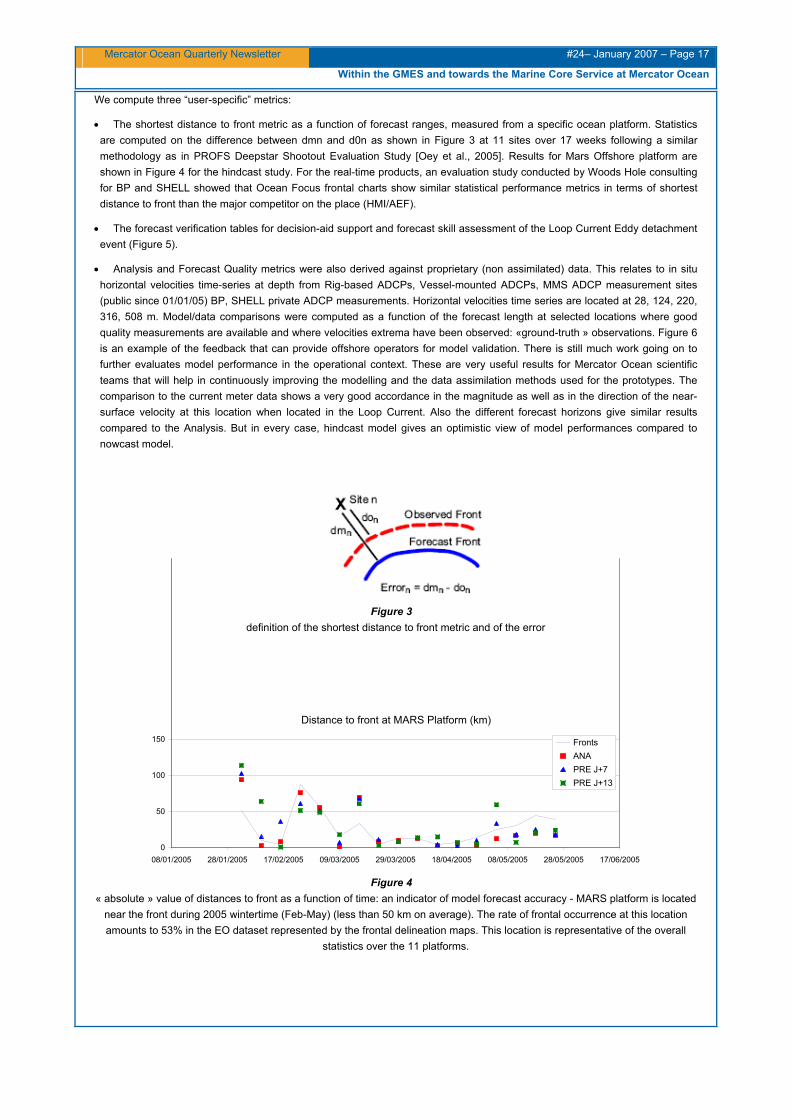
• The shortest distance to front metric as a function of forecast ranges, measured from a specific ocean platform. Statistics are computed on the difference between dmn and d0n as shown in Figure 3 at 11 sites over 17 weeks following a similar methodology as in PROFS Deepstar Shootout Evaluation Study [Oey et al., 2005]. Results for Mars Offshore platform are shown in Figure 4 for the hindcast study. For the real-time products, an evaluation study conducted by Woods Hole consulting for BP and SHELL showed that Ocean Focus frontal charts show similar statistical performance metrics in terms of shortest distance to front than the major competitor on the place (HMI/AEF).
• The forecast verification tables for decision-aid support and forecast skill assessment of the Loop Current Eddy detachment event (Figure 5).
• Analysis and Forecast Quality metrics were also derived against proprietary (non assimilated) data. This relates to in situ horizontal velocities time-series at depth from Rig-based ADCPs, Vessel-mounted ADCPs, MMS ADCP measurement sites (public since 01/01/05) BP, SHELL private ADCP measurements. Horizontal velocities time series are located at 28, 124, 220, 316, 508 m. Model/data comparisons were computed as a function of the forecast length at selected locations where good quality measurements are available and where velocities extrema have been observed: «ground-truth » observations. Figure 6 is an example of the feedback that can provide offshore operators for model validation. There is still much work going on to further evaluates model performance in the operational context. These are very useful results for Mercator Ocean scientific teams that will help in continuously improving the modelling and the data assimilation methods used for the prototypes. The comparison to the current meter data shows a very good accordance in the magnitude as well as in the direction of the near-surface velocity at this location when located in the Loop Current. Also the different forecast horizons give similar results compared to the Analysis. But in every case, hindcast model gives an optimistic view of model performances compared to nowcast model.
Figure 3
definition of the shortest distance to front metric and of the error
« absolute » value of distances to front as a function of time: an indicator of model forecast accuracy - MARS platform is located near the front during 2005 wintertime (Feb-May) (less than 50 km on average). The rate of frontal occurrence at this location amounts to 53% in the EO dataset represented by the frontal delineation maps. This location is representative of the overall
statistics over the 11 platforms.
Mercator Ocean Quarterly Newsletter #24– January 2007 – Page 18
Within the GMES and towards the Marine Core Service at Mercator Ocean
Numbers of MARS Model (ANA/F7/F14)
Occurrences platform outside inside
outside 7/7/7
Correct rejection
1/1/1
False Alarm
EO
Fronts
Inside 2/2/3
Miss
7/7/6
Hit ure 5 MARS location » over 17 weeks: an indicator of mod
FigContingency tables for the event « frontal occurrence at the el forecast
e
records - Red line/Green Line /Blue line : alternate color ting the succession of 14 days of model forecasts issued
Conclusion
s how Mercator Ocean can provide indispensable, useful and high quality Marine Core services to some Downstream services such as Ocean climate monitoring, seasonal prediction and support to offshore industry. The Seventh
performanc
Figure 6
ADCP velocities at 50 m vs. model surface velocities magnitude (upper panel) + direction (lower panel) Black line: ADCP
2005 Wintertime period (Feb-May)
Public ADCP
s represenweekly (warning : High frequencies are not filtered)
This paper illustrate
Framework Programme for research and technological development (FP7) was adopted and first calls for proposals were published late December 2006. Mercator Ocean is coordinating the European partners for the preparation and submission in June 2007 of the proposal answering the FP7 in order to further build the GMES services. Challenges are huge and a lot of work still has to be done but Mercator Ocean is already working to meet the expectations of the Marine Core Service.
Data*
Mercator Ocean Quarterly Newsletter #24– January 2007 – Page 19
Within the GMES and towards the Marine Core Service at Mercator Ocean
Acknowledgements
The authors thanks Ocean Numerics (Robin Stephens, Stephen Wells, Fabien Lefevre) for providing the composite frontal chart and the model/data comparisons plots. Sea surface velocity timeseries come from moored buoys of the National Data Buoy Centre (http://ndbc.noaa.gov).
References
Candela J., S. Tanahara, M. Crepon, B. Barnier, 2003, Yucatan channel flow: observations versus CLIPPER ATL6 and MERCATOR PAM models, Journal of Geophysical Research, 108(C12), 3385.
Ferry, N., 2004: PSY2G: moving towards global operational oceanography. Mercator Newsletter #13. Available at: http://www.mercator-ocean.fr/documents/lettre/lettre_13_art2_en.pdf
Crosnier L, C. Le Provost and Mersea team, 2005, Internal metrics definition for operational forecast systems inter-comparison: Examples in the North Atlantic and Mediterranean Sea, in “Ocean Weather Forecasting : An integrated view of oceanography”, GODAE BOOK Nov 2005 Edited by E. Chassignet and J. Verron, pp457-468, Springer, Kluwer Academic publishers.ftp://oceanmodeling.rsmas.miami.edu/eric/GODAE_Scholl/GODAE_Book
Oey, L.-Y., T. Ezer, G. Forristall, C. Cooper, S. DiMarco, and S. Fan (2005) : "An exercise in forecasting loop current and eddy frontal positions in the Gulf of Mexico", Geophys. Res. letters, VOL 32, L12611, doi:10.1029/2005GL023253
Reynolds, R.W., N.A. Rayner, T.M. Smith, D.C. Stokes, and W. Wang, 2002: An Improved In Situ and Satellite SST Analysis for Climate. J. Climate, 15, 1609-1625.
Saji N.H., Goswami B.N., Vinayachandran P.N. and T. Yamagata, 1999, A Dipole Mode in the Tropical Indian Ocean, Nature, vol. 401, p360-363, 23 September 1999.
Shay, L.K., G. J. Goni and P. G. Black: Effects of Warm Oceanic Features on Hurricane Opal, Month. Weath. Rev., 128, 131-148, 2000.
Sylvie Giraud St Albin, L. Crosnier and R. Stephens, 2005: “A Model Evaluation with new Multivariate Multi-data Mercator Ocean High Resolution Assimilation System to Forecast Loop Current and Eddy Frontal Positions in the Gulf of Mexico”, published in Lettre trimestrielle Mercator Ocean # 19, Octobre 2005 available on http://www.mercator-ocean.fr/html/mod_actu/module/affiche_actualite.php3?idActualite=92&langue=fr
Mercator Ocean Quarterly Newsletter #24– January 2007 – Page 20
BLUElink>delivers first ocean forecasts
BLUElink> delivers first ocean forecasts By Gary B. Brassington1, Andreas Schiller2, Peter R. Oke2, Tim. Pugh1 and Graham Warren1 1 Bureau of Meteorology – BMRC, GPO Box 1289K. Melbourne, Victoria 3001 (Australie) 2 CSIRO Marine and Atmosperic Research – Castray Esplanade, GPO Box 1538. Hobart, TAS 7001 (Australie)
The first global ocean forecasts from the BLUElink> ocean prediction system were delivered in January 2007. Establishing routine ocean forecasts is the concluding stage of a three and a half year research and development project, initiated by the Australian government in 2003. The project was conducted through a collaboration between the Australian Commonwealth Bureau of Meteorology, the Commonwealth Scientific and Industrial Research Organisation and the Royal Australian Navy. The operational prediction system will be delivered through the Bureau of Meteorology to service the Royal Australian Navy, CSIRO and the broader Australian marine user community as a public service. In addition, the prediction system will contribute to the Global Ocean Data Assimilation Experiment including inter-comparisons with Mercator Ocean.
Introduction
The primary goal of the BLUElink project is to deliver operational short-range ocean forecasts for the Asian-Australian region. The BLUElink project was undertaken by a team of scientists, technicians and naval officers drawn from the Australian Commonwealth Bureau of Meteorology (CBoM), the Commonwealth Scientific and Industrial Research Organisation (CSIRO) and the Royal Australian Navy (RAN). The project included research and development for a comprehensive range of ocean related activities including: (1) an ocean observational data management systems, (2) product visualisation, (3) internet data access services, (4) high resolution regional climatology, (5) high resolution regional analyses, (6) high resolution sea surface temperature analyses, (7) surface wind verification, (8) global OGCM with eddy resolving resolution in the region, (9) data assimilation system for an eddy-permitting OGCM, (10) a 15 year ocean reanalysis, (11) an intermediate global model, (12) an experimental regional ocean and coupled model, (13) a real-time quality control system, (14) an operational forecast system and (15) a relocatable ocean model. Only a subset of these components is discussed further in this article. For more introductory information on the BLUElink project please refer to [12].
BLUElink> is a partner to the Global Ocean Data Assimilation Experiment (GODAE,[13]) a project designed to encourage and support the development of data assimilating ocean prediction systems around the world. GODAE has promoted the sharing of data, the standardising of forecast metrics, the use of common data formats and protocols for data servicing. The BLUElink> operational forecast system as a partner has been able to establish “operational” real-time observational data streams and develop data services based on GODAE and IOOS conventions.
The operational ocean forecast system comprises several software components including (a) the Ocean Forecast Australia Model (OFAM), (b) the BLUElink> Ocean Data Assimilation System (BODAS;[1]), (c) an in situ observational data processing system and (d) a atmospheric flux processing and regridding system. The system relies on several high quality input data products including real-time observations, operational atmospheric forecasts, ocean climatologies and bathymetry products. The system has been configured to run at the CBoM taking advantage of operational infrastructure including high performance computing systems, real-time communications systems and data management and archival systems. This article will briefly outline the specific software, data products and infrastructure used in the Ocean Model, Analysis and Prediction System (OceanMAPS;[2]) together with some measures of performance.
Software components
Ocean Forecast Australia Model (OFAM)
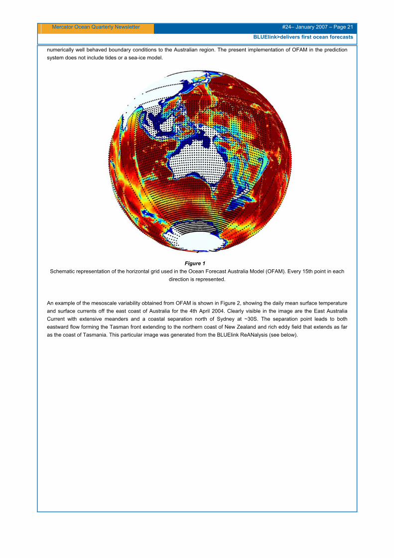
BLUElink> have implemented the GFDL Modular Ocean Model version 4 p0d (MOM4) [8] with specific enhancements for mixed layer physics [9] and the algorithm for calculating penetrative solar radiation. In addition, the software includes some enhancements to vectorise routines for use on the NEC SX6 high performance computing facility. OFAM uses a global grid with a horizontal resolution of 0.1°×0.1° in the Australian region defined by 90E-180E and 75S-16N which is designed to resolve mesoscale ocean dynamics. Outside this region the grid is stretched up to a resolution of 0.9° in the Indian Ocean and South Pacific Ocean and tropical North Pacific. Beyond this domain the resolution in the North Atlantic is 2°×2°. A schematic representation of the horizontal grid that illustrates the concentration of grid points in the Australian region is shown in Figure.1. OFAM has 47 vertical levels with the top 20 levels uniformly distributed at 10m resolution. Below 200m, the vertical grid spacing is increased to bottom cell spacing of 962m and a total depth of 5000m. This configuration has 71% of the total grid points within the Australian region and 72% of all model grid points are water cells. The OFAM grid provides dynamically consistent and
Mercator Ocean Quarterly Newsletter #24– January 2007 – Page 21
BLUElink>delivers first ocean forecasts
numerically well behaved boundary conditions to the Australian region. The present implementation of OFAM in the prediction system does not include tides or a sea-ice model.
Figure 1 Schematic representation of the horizontal grid used in the Ocean Forecast Australia Model (OFAM). Every 15th point in each
direction is represented.
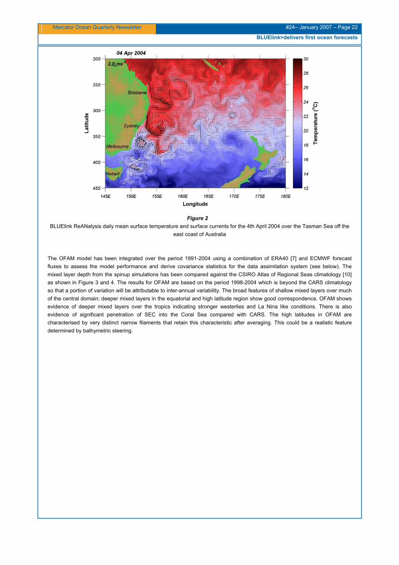
An example of the mesoscale variability obtained from OFAM is shown in Figure 2, showing the daily mean surface temperature and surface currents off the east coast of Australia for the 4th April 2004. Clearly visible in the image are the East Australia Current with extensive meanders and a coastal separation north of Sydney at ~30S. The separation point leads to both eastward flow forming the Tasman front extending to the northern coast of New Zealand and rich eddy field that extends as far as the coast of Tasmania. This particular image was generated from the BLUElink ReANalysis (see below).
Mercator Ocean Quarterly Newsletter #24– January 2007 – Page 22
BLUElink>delivers first ocean forecasts
Figure 2 BLUElink ReANalysis daily mean surface temperature and surface currents for the 4th April 2004 over the Tasman Sea off the
east coast of Australia
The OFAM model has been integrated over the period 1991-2004 using a combination of ERA40 [7] and ECMWF forecast fluxes to assess the model performance and derive covariance statistics for the data assimilation system (see below). The mixed layer depth from the spinup simulations has been compared against the CSIRO Atlas of Regional Seas climatology [10] as shown in Figure 3 and 4. The results for OFAM are based on the period 1998-2004 which is beyond the CARS climatology so that a portion of variation will be attributable to inter-annual variability. The broad features of shallow mixed layers over much of the central domain; deeper mixed layers in the equatorial and high latitude region show good correspondence. OFAM shows evidence of deeper mixed layers over the tropics indicating stronger westerlies and La Nina like conditions. There is also evidence of significant penetration of SEC into the Coral Sea compared with CARS. The high latitudes in OFAM are characterised by very distinct narrow filaments that retain this characteristic after averaging. This could be a realistic feature determined by bathymetric steering.
Mercator Ocean Quarterly Newsletter #24– January 2007 – Page 23
BLUElink>delivers first ocean forecasts
Figure 3 Depth of the temperature that is 1.0°C cooler than the surface. (a) mean January from CARS, (b) mean January from OFAM
based on 1998-2004
Figure 4 Depth of the temperature that is 1.0°C cooler than the surface. (a) mean July from CARS, (b) mean July from OFAM based on
1998-2004
BLUElink> Ocean Data Assimilation System (BODAS)
BLUElink> has developed a new software to perform ocean data assimilation which uses an ensemble based, multi-variate optimal interpolation scheme [1]. A specific feature of the scheme is the use of an ensemble of anomalies from the seasonal cycle generated from a spinup integration of OFAM to estimate the background error covariances. The first comprehensive examination of this scheme was through a 15 year (1992-2004) BLUElink ReANalysis (BRAN) which used a 72 member ensemble. In general, the undersampling of the covariance statistics can contain large values far from the point of interest. These were assumed to be unrealistic features for mesoscale variability and were controlled through localisation. It is critical to this scheme that the free ocean model driven by surface fluxes is able to maintain both a realistic mean ocean state and a realistic distribution of ocean variability. A complete analysis of OFAM is a significant on-going task.
Mercator Ocean Quarterly Newsletter #24– January 2007 – Page 24
BLUElink>delivers first ocean forecasts
A comparison of the statistics of the model anomalies with the statistics found in satellite altimetry observations is shown in Figure 5. The correlation between modelled sea surface height anomalies at Thevenard (133.65E, 32.15S) in Southern Australia with sea surface height anomalies in the surrounding region is shown in Figure 5a. The region of high correlation is confined to the continental shelf (<200m) and elongated along the coastline. Also shown in Figure 5a are the correlations of sea surface height anomalies from the available coastal tide gauge (ctg) network with the ctg located at Thevenard. The ctg time series have been filtered for tides and the seasonal cycle and the correlations show good agreement with those of OFAM. In Figure 5b, the sea surface height anomalies of Topex-Poseidon are correlated with those of the ctg at Thevenard. Again the region of high correlation is confined to the continental shelf and elongated along the coastline in good agreement with the statistics represented by the model. This pattern is consistent for both Jason1 and GFO (not shown). This analysis indicates that (1) OFAM is reproducing observed variability of sea level height anomalies, (2) the statistics of sea surface height anomalies change in character across the 200m isobath, (3) there is signal in both the ctg’s and the satellite altimetry in the coastal zone and (4) the strategy of using model based covariances from OFAM will separate the influence of coastal and open ocean innovations consistent with observations. Indeed, the use of covariances that do not account for the anisotropic scales in this region will lead to poor quality analyses in the cross shelf region. The common alternative practice is to reject observations within the 200m isobath. The region of Thevenard is a particularly good example because it is characterised by a large continental shelf but a relatively modest tidal signal. Both the North West Shelf and the continental shelf off Queensland do not exhibit the same level of correlation and are characterised by significant tidal signals. However strong relationships are found for all tide gauges on the Australian coast that have a weak tidal signal. Further research is being conducted into region where the tidal signal is larger.
Figure 5 (a) Correlation of OFAM seasonal anomalies of sea surface height at Thevenard with anomalies in the Australian region. The
circles correspond to correlations of observed seasonal sea surface height anomalies from coastal tide gauges to that of Thevenard. (b) correlation of seasonal filtered sea surface height anomalies from the Thevenard coastal tide gauge and the
surrounding seasonally filtered sea surface height anomalies observed by Topex-Poseidon
In situ observation processing system
The GTS is the primary operational communication for in situ ocean observations received by the CBoM. Both the BATHY and TESAC messages are reformatted to an Argo netCDF format. A priority for BLUElink> has been to ensure the maximum number of Argo retrievals available in real-time. The Argo observations are distributed in real-time through the GTS without quality control and subsequently distributed through two global data assembly centres (USGODAE and Coriolis) with automatic quality control. Processing of the three sources Argo files has consistently revealed that none of these sources contain a complete superset of all the real-time observations. In order to maximise the quantity of Argo observations a duplicate checker was developed to locate all duplicates and form a single file containing the best copy (the highest level of quality control) amongst the duplicates for each day.
The best daily observation files preserve all of the available quality control messages from the automatic QC performed at the DAC’s. Each best daily observation file is further processed using an internal set of quality control checks including standard checks for monotonicity, stability as well as some of the checks from [11] plus comparisons with climatology.
Flux regridder
A regridding software was developed to provide a conservative regridding with a new approach introduced to remap atmospheric features aligned with the coastline on a coarse grid with the coastline of a higher resolution target grid. This was
(a) (b)
Mercator Ocean Quarterly Newsletter #24– January 2007 – Page 25
BLUElink>delivers first ocean forecasts
developed to regrid the Bureau’s GASP forecasts with a resolution of 0.75 degrees to the OFAM grid with resolution up to 1/10 degree. A sample of 6 hour averaged longwave radiation from the GASP model for 12 February 2006 is shown in Figure 6. After applying the full regridding algorithm the downscaled fluxes for this region are shown in Figure 7. The sea-ice mask is regridded and used to apply zero mass, momentum and heat flux.
Figure 6 GASP longwave radiation, 12 Feb 2006, shown on the source grid over the Tasman Sea and Bass Strait
Figure 7 GASP longwave radiation with adjustment of the GASP coastline land mask to the OFAM mask coastline
Mercator Ocean Quarterly Newsletter #24– January 2007 – Page 26
BLUElink>delivers first ocean forecasts
Data products
Observation products
The Bureau of Meteorology receives BATHY and TESAC messages via the GTS which are composed of XBT, Moored CTD’s and Argo without quality control. These observations are close to real-time with 90% observing the ocean with the past 3 days. The Bureau also retrieves Argo data products from the two GDAC’s USGODAE and Coriolis via ftp. These products contain Argo observations that have undergone automated quality control. Both GDACs contain observations that span a larger number of days but typically 90% within the past 7 days.
At present there are two satellite altimeters available for operational oceanography, Jason and Envisat. OceanMAPS does not process the raw satellite altimetry observations but instead retrieves processed sea surface height anomaly products from JPL and ESA. The quality of these products is impacted by the algorithm used to compute the Geophysical Data Record. The faster algorithms required for the near real-time delivery impact the quality of the products. Sensitivity of analyses to real-time ssha products has not been assessed.
Each of the sources of sea level anomaly products are obtained in a unique way. Jason is obtained via OCEANIDS and ftp push service provided by PO.DAAC. ENVISAT is obtained via an ftp push from ESA. Each data stream has its own unique file format which is processed at the Bureau and passed through a series of quality control checks and reformatted to BUFR for storage and netCDF for use in the analysis.
Surface products
The Bureau maintain a set of operational NWP forecast systems including: GASP [3] a global assimilation and prediction system based on a spectral model and LAPS [4] a limited area prediction system for the Australian region. GASP has a maximum horizontal resolution of 0.75°×0.75° resolution in the tropics and uses a gaussian grid in high latitudes and has 33 sigma levels. The analysis uses a generalised multi-variate statistical interpolation scheme (GenSI) which has been recently upgraded to include scatterometer observations from QuikSCAT. The analysis for GASP is performed on a 6 hourly cycle with 10day forecasts issued every 12 hours at 06Z and 18Z. Analyses have demonstrated modest improvements in bias and skill in forecast winds [5, 6]. GASP fluxes are retrieved from the operational disk storage and regridded to the OFAM grid.
The Bureau of Meteorology has also recently upgraded its regional sea surface temperature analysis system to a twice daily, high resolution (1/12 by 1/12) operational product. The analysis system developed under BLUElink makes use of available AVHRR, AATSR and AMSR-E satellite retrievals calibrated to a common foundation using a GHRSST strategy. The prediction system at present applies a 30 day relaxation to the sea surface temperature analyses.
Other datasets
High resolution, accurate bathymetry for OFAM was produced by combining global products of the US Navy with the regional products of Geoscience Australia for the Australian region. In addition, the system makes use of both the CARS2005 and WOA2005 climatological datasets for quality control and for deep restoring.
Operational infrastructure
The Bureau maintains communications with a variety of networks including GTS, Internet, Grangenet, AARNet2 to support NRT observation retrievals and data distribution. The majority of ocean profile observations are obtained from the GTS. Satellite observations such as sea surface anomalies from JASON-1 are available between 5-7hrs behind real-time either on GODAE servers in a pull mode or for operational centres such the Bureau in a push mode. Topex-Poseidon is also available from OCEANIDS but is available approximately 18hrs behind real-time. Recent observations are collected into over-written files in local memory and later archived.
The Bureau has recently implemented the Meteorological Archival and Retrieval System (MARS) to serve as the primary meteorological database. This system was developed by ECMWF and was designed for storage of NWP output. The system supports two file formats Gridded Binary (GRIB) and Binary Universal Form for the Representation of meteorological data (BUFR) which are specific formats developed by ECMWF for the meteorological community that provide good compression. However, neither of these two formats are widely used or supported outside this community by other centres or software developers. For example, OPeNDAP does not provide support for reading these file formats and there are no plans from the OPeNDAP developers to include this format in future. The Bureau has developed code to convert between file formats such as NetCDF and GRIB and BUFR.
Mercator Ocean Quarterly Newsletter #24– January 2007 – Page 27
BLUElink>delivers first ocean forecasts
The OFAM model’s performance on the NEC SX6 has been measured during two ocean model only integrations (so called “spinup”) using ERA40. The first integration was performed using MOM4p0b, which included the leap-frog time integration scheme and neutral physics using a baroclinic timestep of 300s. This was performed on 21 processors across 3 nodes sustaining 10.8 Gflops. The second integration was performed using MOM4p0d, which included a new time integration scheme and with neutral physics switched to false using a baroclinic timestep of 600s. This was performed on 42 processors across 6 nodes sustaining 31.8 Gflops demonstrating some problems in scalability of the MOM software. The resource values are summarised in Table 1. The MOM4 core code scales well across both the NEC-SX6 and several other platforms. However, the I/O performance does scale on any of the benchmarked platform and can lead to performance deterioration.
Spinup I Spinup II
Nodes 3 6
Cpu’s (total) 21 42
Memory(total) ~86GBytes ~114GBytes
Cputime/model day 20 minutes 11.5 minutes
Sustained flops (total) 20.3 Gflops 31.8 Gflops
Table 1 Performance of OFAM (MOM4) on the NEC SX6
Prediction system
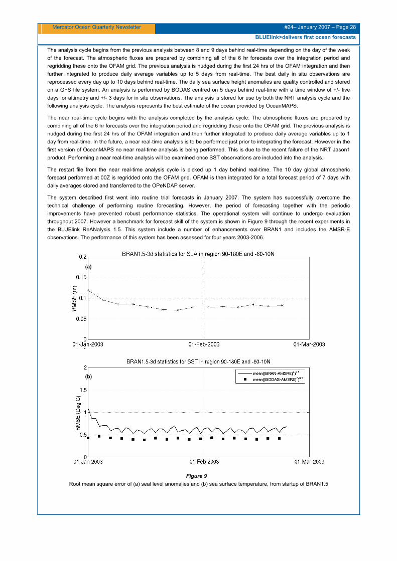
The OceanMAPS system is performed in three sequential phases. The first phase is the analysis cycle which produces an analysis 5 days behind real-time that is the best estimate of the ocean state, the second phase is the near real-time analysis cycle which integrates OFAM forward to produce an analysis 1 day behind real-time and the final phase is the forecast cycle which integrates forward for 7 days. The entire cycle is performed twice per week on Mondays and Thursdays. A schematic of the recent schedule is shown in Figure 8.
Figure 8 A schematic of the calendar schedule for the three cycles performed in OceanMAPS.
Mercator Ocean Quarterly Newsletter #24– January 2007 – Page 28
BLUElink>delivers first ocean forecasts
The analysis cycle begins from the previous analysis between 8 and 9 days behind real-time depending on the day of the week of the forecast. The atmospheric fluxes are prepared by combining all of the 6 hr forecasts over the integration period and regridding these onto the OFAM grid. The previous analysis is nudged during the first 24 hrs of the OFAM integration and then further integrated to produce daily average variables up to 5 days from real-time. The best daily in situ observations are reprocessed every day up to 10 days behind real-time. The daily sea surface height anomalies are quality controlled and stored on a GFS file system. An analysis is performed by BODAS centred on 5 days behind real-time with a time window of +/- five days for altimetry and +/- 3 days for in situ observations. The analysis is stored for use by both the NRT analysis cycle and the following analysis cycle. The analysis represents the best estimate of the ocean provided by OceanMAPS.
The near real-time cycle begins with the analysis completed by the analysis cycle. The atmospheric fluxes are prepared by combining all of the 6 hr forecasts over the integration period and regridding these onto the OFAM grid. The previous analysis is nudged during the first 24 hrs of the OFAM integration and then further integrated to produce daily average variables up to 1 day from real-time. In the future, a near real-time analysis is to be performed just prior to integrating the forecast. However in the first version of OceanMAPS no near real-time analysis is being performed. This is due to the recent failure of the NRT Jason1 product. Performing a near real-time analysis will be examined once SST observations are included into the analysis.
The restart file from the near real-time analysis cycle is picked up 1 day behind real-time. The 10 day global atmospheric forecast performed at 00Z is regridded onto the OFAM grid. OFAM is then integrated for a total forecast period of 7 days with daily averages stored and transferred to the OPeNDAP server.
The system described first went into routine trial forecasts in January 2007. The system has successfully overcome the technical challenge of performing routine forecasting. However, the period of forecasting together with the periodic improvements have prevented robust performance statistics. The operational system will continue to undergo evaluation throughout 2007. However a benchmark for forecast skill of the system is shown in Figure 9 through the recent experiments in the BLUElink ReANalysis 1.5. This system include a number of enhancements over BRAN1 and includes the AMSR-E observations. The performance of this system has been assessed for four years 2003-2006.
Figure 9 Root mean square error of (a) seal level anomalies and (b) sea surface temperature, from startup of BRAN1.5
(a)
(b)
Mercator Ocean Quarterly Newsletter #24– January 2007 – Page 29
BLUElink>delivers first ocean forecasts
The principle user of the operational products and joint-partner in the project is the RAN. RAN have direct access to the full suite of data products from which they perform direct visualisation as well as downscale the information through a relocatable ocean model capability developed by CSIRO. In addition to RAN, the operational system is being developed at the Bureau as a general public service for the benefit of the wider Australian maritime community. Australia is an island continent surrounded by three of the worlds major oceans. Australia’s 200nm Exclusive Economic Zone ranks as the third largest in the world behind the United States and France. Guiding the sustainable management of this vast resource is a critical activity for the Australian government. Important users will include: the Australian Maritime Safety Authority for ocean surface tracking; marine management such as the Great Barrier Reef Marine Park Authority; oil and gas industry as well as numerous tourism and recreational users. Establishing the user community and development of the products and services for the community will be an on-going activity for BLUElink>.
Conclusion
The three-year targets of the BLUElink> project will be concluded in early 2007 having established a range of new and improved software and data products together with the introduction of a new ocean prediction system within the Bureau of Meteorology delivering routine 7 day forecasts, twice per week. This system will continue to undergo minor refinements and thorough evaluation throughout 2007. The successful scientific partnership between the Bureau of Meteorology research centre and CSIRO is set to continue with a three year project extension. The key research areas will be further optimisation of the ocean prediction system through extension to the observation types analysed, optimisation of the data assimilation system and enhancements to the ocean model with a focus on improving skill in the coastal regions. Other research areas will include research and development for a coupled limited area model exploring ocean-wave-atmosphere coupling and developing an operational coupled tropical cyclone forecasting system and research into an operational version of SWAN.
Acknowledgements
This research is supported by the BLUElink> project, Bureau of Meteorology, CSIRO and the Royal Australian Navy. Atmospheric analyses were provided by ECMWF, satellite altimetry is provided by NASA, CNES, ESA and NOAA. Bathymetry is derived from datasets from Geoscience Australia and the US Navy.
References
Oke, P. R., A. Schiller, D. A. Griffin and G. B. Brassington, 2005: Ensemble data assimilation for an eddy-resolving ocean model of the Australian region, Q. J. R. Meteorol. Soc., 131, 3301-3311.
Brassington, G. B., P. R. Oke and T. Pugh, 2006: BLUElink> Operational ocean prediction in Australia, pp87-95, in Advances in Geosciences, Volume 5: Ocean and Atmospheres (OA), Eds. H. Choi and M. Speers, World Scientific Publishing
Seaman, R., Bourke, W., Steinle, P., Hart, T., Embery, G., Naughton, M and Rikus, L., Evolution of the Bureau of Meteorology's Global Assimilation and Prediction System, Part 1: Analyses and Initialization, Aust. Met. Mag., 44, 1-18, 1995.
Puri, K., Dietachmayer, G., Mills, G. A., Davidson, N. E., Bowen, R. A. and Logan, L. W., The new BMRC Limited Area Prediction System, LAPS, Aust. Met. Mag., 47, 203-233, 1998.
Kepert, J. D., D J M Greenslade and G D Hess. Assessing and improving the marine surface winds in the Bureau of Meteorology numerical weather prediction systems. BMRC Research Report No. 10, 2005.
Schulz E. W., Jeffrey D. Kepert, and Diana J. M. Greenslade , An Assessment of Marine Surface Winds in Numerical Weather Prediction Systems at the Australian Bureau of Meteorology. Weather and Forecasting (in press)
Kallberg, P., A. Simmons, S. Uppala, and M. Fuentes, 2004: The ERA-40 archive. ERA-40 Project report series no 17, ECMWF.
Griffies, S. M., M J Harrison, R C Pacanowski, and A Rosati, ‘A technical guide to MOM4’. GFDL ocean group technical Report No. 5, 339pp, 2004.
Chen. D., L M Rothstein and A J Busalacchi. ‘A hybrid vertical mixing scheme and its application to tropical ocean models’. J. Phys. Oceanogr., 24, pp2156-2179, 1994.
Ridgway K.R., J.R. Dunn, and J.L. Wilkin, Ocean interpolation by four-dimensional least squares -Application to the waters around Australia, J. Atmos. Ocean. Tech., Vol 19, No 9, 1357-1375, 2002
Mercator Ocean Quarterly Newsletter #24– January 2007 – Page 30
BLUElink>delivers first ocean forecasts
Ingleby, B. and M. Huddleston, 2006: Quality control of ocean temperature and salinity profiles – historical and real-time data, J. Mar. Sys., (to appear)
Macaulay, C. and A. Schiller, 2004: Australia’s Bluelink project approaches first milestone, Projection Mercator, 4, 7 http://www.mercator-ocean.fr/documents/actualites/projection/Projection_n4_en.pdf.
Smith N. and M. Lefebvre, 1997, The Global Ocean Data Assimilation Experiment (GODAE). Monitoring the oceans in the
2000s: An integrated approach. International Colloque, Biarritz, October 15-17, 1997.
Mercator Ocean Quarterly Newsletter #24– January 2007 – Page 31
GODAE at work in the Indian Ocean and Australian Area
GODAE at work in the Indian Ocean and Australian Area: Metrics definition and intercomparison of the BLUELink and Mercator systems. By: Laurence Crosnier1, Garry B. Brassington2, Marie Drevillon3, Edmée Durand1 and Fabrice Hernandez1
1Mercator Ocean - 8-10 rue Hermes, Parc technologique du Canal. 31526 Ramonville St Agne 2BLUELink, Bureau of Meteorology – BMRC, GPO Box 1289K. Melbourne, Victoria 3001 (Australie) 3Mercator Ocean (Cerfacs) - 8-10 rue Hermes, Parc technologique du Canal. 31526 Ramonville St Agne
Introduction
The methodology to achieve a real time inter-comparison of operational forecast systems for the Indian Ocean within the GODAE framework is presented. The main objective of the inter-comparison exercise is to show the strengths and weaknesses of each system according to the specificity and strategy adopted, as well as to provide guidance for improving future operational systems. A standard set of diagnostics called metrics, first developed within the MERSEA European framework, has been adopted by the international GODAE community. Such metric definitions aim to systematically assess the quality, consistency and performance of each system (Le Provost, 2002), whereby:
•
•
•
•
‘Consistency’ means that operational systems outputs have to be consistent with the current knowledge of the ocean circulation and climatologies.
‘Quality’ means that operational systems outputs have to be in agreement with independent observations (i.e. not assimilated).
‘Performance’ means that metrics should quantify the capacity of each system to provide accurate short term forecast.
For MFS (Mediterranean Ocean Forecasting System) assessment, [Pinardi and Tonani, 2005] proposed a fourth principle, to verify and take into account the interest/relevance for the customer, and catch intermediate- or end-users feedbacks:
‘Benefit’: user assessment of which quality level has to be reached before the product is useful for an application.
For the last two years, the Mercator Ocean team in charge of the Global forecasting system within the MERSEA framework have been discussing with Japanese [Kamachi, 2004] and Australian [Oke and Brassington, 2005] groups, in order to define the Pacific and Indian Ocean metrics respectively. This paper is describing the Indian Ocean and Australian Region metrics defined collectively by the French Mercator Ocean (Crosnier and Hernandez, 2006) and Australian BLUElink [Oke and Brassington, 2005] teams. We are also showing some preliminary results for the inter-comparison exercise of the Mercator Ocean and BLUELink systems.
The Mercator Ocean and BLUELink systems
The French Mercator Ocean global system ¼° PSY3V1 used in this study has been described in a previous issue (issue N°19 of the Newsletter) in October 2005. The Australian BLUElink system is described in this issue in a companion paper.
Metrics in the Indian Ocean
The Class 1, 2 and 3 metrics for the Indian Ocean and Australian Area are listed in Table 1 and illustrated in Figure 1.
Mercator Ocean Quarterly Newsletter #24– January 2007 – Page 32
GODAE at work in the Indian Ocean and Australian Area
METRIC CLASS
Daily mean best estimate and 6th day forecast fields provided for the following variables:
CLASS 1 3D fields:
Temperature (oC)
Salinity (psu)
Zonal current (m/s)
Meridional Current (m/s)
CLASS 1 2D fields:
Zonal and meridional wind stress (Pa),
Total net heat flux including relaxation temp (W/m2),
Freshwater flux, including relaxation term (kg/m2/s),
Mixed Layer Depth (MLD) (m). Two kinds of MLD diagnostics are provided: MLD(θ) with a 0.2oC criteria and MLD(σ) with a 0.03 kg/m3 surface potential density criteria, following DeBoyerMontegut et al. (2004).
Sea-level (SL) (m)
Mean sea-level (MSL) (m)
CLASS 2 Potential Temperature (oC)
Salinity (psu)
Zonal current (m/s)
Meridional Current (m/s)
Sea-level (m)
CLASS 3 Volume transports (Sv)
Section-normal temperature flux (oC kg m-2)
Section-normal salt flux (psu kg m-2)
Table 1 Class 1, 2 and 3 metrics in the Indian Ocean and Australian Area.
Figure 1 shows the positions of the class 2 sections in the Indian Ocean and Australian region. Figure (1, top panels) shows the Class2 “straight” and “XBT” sections. Their location is chosen according to the existing WOCE/CLIVAR sections, to the SOOP program, as well as to the physical processes taking place in the studied area. They will allow the assessment of, among other processes, the representation of the Leeuwin Current system, the Leeuwin Current extension, the Flinders Current and wind-driven upwelling/downwelling off Adelaide, the representation of the transports and properties of the East Australian Current, the transports and properties of the Indonesian Throughflow waters, the representation of the equatorial wave guide, the transports and properties of the Aghulas Current System and the Antarctic Circumpolar Current, the saline flux discharge from the Red Sea, the freshwater discharge from the Bay of Bengal.
The mooring positions in the equatorial Indian Ocean (Figure 1, bottom left panel, green dots) correspond to the locations proposed by the Indian Ocean Panel for a sustained observing system that is similar to the TAO array (http://www.pmel.noaa.gov/tao/disdel/disdel.html). Next section illustrates the comparison of the Mercator Ocean systems with the TAO moorings at 80.5°E and 90°E. Tide gauge moorings from the GLOSS data base (Figure 1, blue dots) (http://ilikai.soest.hawaii.edu/uhslc/woce.html) are also indicated. Black dots (Figure 1) correspond to the NIOT moorings (http://www.niot.res.in/ndbp/index.html), and red dots (Figure 1) to the OceanSites moorings (http://www.oceansites.org).
Moorings, Red dots: Oceansites Moorings, Blue dots: GLOSS tide gauges, Green dots: TAO Moorings).
Preliminary results for the inter-comparison exercise of the Mercator Ocean and BLUELink systems.
In this section, we present preliminary results of the comparison of the BLUElink and Mercator Ocean systems with observations.
First, we compare the Mercator Ocean and BLUELink system extracted along the WOCE section track to a historical WOCE synoptic section (I08S-I09N from Dec. 94 to March 95). The WOCE program gathered in situ data during the 90’s, a time period that is not synchronous with the MERSEA/GODAE exercises. Nevertheless, the comparison with WOCE sections brings relevant insights on the systems water masses characteristics. Figure 2 displays a potential temperature and salinity sections in the Indian Ocean at 95°E from the WOCE/CLIVAR program, the BLUELink and Mercator Ocean systems and Levitus climatology.
The Indian Ocean WOCE salinity section (I09N and I08S) at 95°E (Figure 2) displays the following water masses: The North-south section of properties shows the high salinity evaporation region of the South subtropical gyre (with its equatorward subsurface salinity maximum, the Subtropical Underwater extending from 35°S to 10°S). Below the saline surface layer is the salinity minimum of the Antarctic Intermediate Water (AAIW). In the South Indian Ocean from 70 to 30°S, the salinity maximum below the AAIW extends northward from the Antarctic Circumpolar Current. Much of the high salinity of this layer comes from its source in the North Atlantic (remnant of North Atlantic Deep Water). At the bottom is the fresher Antarctic Bottom Water or Lower Circumpolar Deep Water. In the North Indian Ocean, the deep-reaching saline water comes from the Red Sea, which is an area of high evaporation where deep water is formed, in a similar way as in the Mediterranean Sea. In the Indian Ocean, the saline water coming from the Red Sea is affecting a deeper layer than the Mediterranean Outflow since there is no denser
Mercator Ocean Quarterly Newsletter #24– January 2007 – Page 34
GODAE at work in the Indian Ocean and Australian Area
northern source of water. There is also a very thin layer of low salinity water at the sea surface in the north of the section, which originates in the Bay of Bengal from monsoon rainfall and from the associated major river runoff into this area, including the Ganges and many other large rivers. Moreover, one can see lower salinity water around 10°S at the surface. This water is connected to a westward flow (also linked to the Leeuwin Current) through the Indonesian archipelago from the Pacific Ocean towards the Indian Ocean western boundary.
The Mercator Ocean and BLUELink sections along 95°E in the Indian Ocean are in good agreement with the WOCE water masses described above, as well as with the Levitus climatology. This reflects a realistic behavior of both systems for a various range of dynamics. The BLUElink section north of the equator is more saline than all other sections and can be accounted for by the absence of river discharge. River discharge based on a climatological database is currently being tested.
WOCE
I08S-I09N
Bluelink
Mercator
Ocean
Mercator Ocean Quarterly Newsletter #24– January 2007 – Page 35
GODAE at work in the Indian Ocean and Australian Area
Levitus
Figure 2 Potential temperature (°C) (left column) and salinity (psu) (right column) along the 95°E meridional section in the Indian Ocean
a) in WOCE Sections I08S and I09N (January 1994 to March 1995), b) in BLUELink Reanalysis in October 2005, c) in Mercator Global PSY3V1 in October 2006, d) in Levitus in October.
Second, we show preliminary results from the comparison of the Indian Ocean TAO observations with the Mercator Ocean and BLUElink systems. An Indian Ocean TAO Mooring observatory (http://www.pmel.noaa.gov/tao/disdel/disdel.html) will soon allow monitoring the observed depth of the thermocline in the equatorial Indian Ocean, as it is already the case in the Pacific Ocean (http://www.pmel.noaa.gov/tao/jsdisplay/ ). In the Indian Ocean, moorings are already available along 80.5°E and 90°E (Figure 3).
We compare the Mercator Ocean Sea Surface Temperature (SST) and Sea Surface Salinity (SSS) to the TAO Moorings SST and SSS along 80.5°E and 90°E (Figures 4 and 5), from September to early December 2006. Reynolds weekly analyzed SST (Reynolds et al. 2002) as well as Levitus SST (Levitus, 1998) are also shown for the same time period. BLUElink SST and SSS are not shown for the time period September to early December 2006, but September to early December 2005, as the reanalysis is not yet available for the end of 2006. They can be compared to the Reynolds weekly analyzed SST for the period September to early December 2005. Further comparison of the 3 fields (Mercator Ocean, BLUElink, TAO observations) for the same time period will take place when all 3 available for synchronous time period.
Figures 4 and 5 show that the SST and SSS at 80.5°E in the Mercator Ocean system is up to 1°C colder and 0.6 psu saltier than observations (TAO and Reynolds). Such bias should be solved in the next version soon to be released of the global Mercator Ocean system where Coriolis temperature and salinity profiles and Sea Surface Temperature will be assimilated, and where Bulk formula fluxes will be applied with a GPCP1 correction of the ECMWF precipitation fluxes. At 90°E however, SST and SSS in the Mercator Ocean system are in very good agreement with observations. The BLUElink SSTs are in good agreement with the Reynolds weekly analyses. Note that the BLUElink system, as explained in a companion paper (this issue), does assimilate temperature and salinity profiles as well as satellite SST from AMSR-E. There are no data presented here to compare the BLUElink SSS with. These comparisons highlight the large interannual variability in this region and particularly that 2006 was an anomalous year for both SST and SSS compared with 2005.
Third, we compare zonal velocities in the top 200 meters along the equator at 80.5°E from both Mercator Ocean and BLUElink systems. Figure 6 shows hovmuller diagram of the zonal velocities in the top 200 meters along (0°N, 80.5°E) in observations for the time period July 1993 to September 1994 [Reppin et al., 1999] and in the Mercator Ocean and BLUElink systems for the time period January to May 2006. We note, in agreement with the observations, an alternation of surface Wyrtki Jets (WJ) [Wyrtki, 1973] as a function of the seasons, reaching very similar amplitude of -0.8 m.s-1 in February 2006, and reversing to 1.4 m.s-1 in April-May 2006 in both Mercator Ocean and BLUElink systems. Further at depth, the Equatorial Under Current (EUC) which is considered as an equatorial wave phenomenon rather than a current, located around the equatorial upper thermocline, flows in the opposite direction than the surface WJ and can be westward or eastward. Between June 1993 and August 1994 [Reppin et al., 1999] (Figure 6, top panel), the monthly-mean zonal current shows an EUC between 50 and 150m from February to May 1994 that disappeared, as expected, in June and reappeared in August at a shallower depth and weaker. Westward flow was observed at the same time during summer 1993. In the Mercator Ocean and BLUElink systems (Figure 6, middle and bottom panels), the EUC is located at a realistic depth (~100-120m). It reaches larger amplitude in the BLUElink (1 m.s-1 in March-April 2006) than in the Mercator Ocean system (0.6 m.s-1 in March 2006).
Mercator Ocean Quarterly Newsletter #24– January 2007 – Page 36
GODAE at work in the Indian Ocean and Australian Area
Figure3 Location of the TAO moorings in the Indian Ocean along 80.5°E and 90°E.
80.5°E 90°E
Levitus
SEPT to DEC
TAO SEPT to DEC
2006
REYNOLDS
SEPT to DEC
2006
MERCATOR
SEPT to DEC
2006
Mercator Ocean Quarterly Newsletter #24– January 2007 – Page 37
GODAE at work in the Indian Ocean and Australian Area
BLUElink
SEPT to DEC
2005
REYNOLDS
SEPT to DEC
2005
Figure4 Hovmuller plot of the Sea Surface Temperature (°C) along longitude (left) 80.5° E, (right) 90°E. From Top to Bottom: LEVITUS
(Sept to Dec), TAO (Sept to Dec 2006), Reynolds (Sept to Dec 2006), Mercator PSY3V1 (Sept to Dec 2006), BLUElink (Sept to Dec 2005), Reynolds (Sept to Dec 2005)
80.5°E 90°E
Levitus
SEPT to DEC
TAO SEPT to DEC
2006
MERCATOR
SEPT to DEC
2006
Mercator Ocean Quarterly Newsletter #24– January 2007 – Page 38
GODAE at work in the Indian Ocean and Australian Area
BLUElink
SEPT to DEC
2005
Figure5 Hovmuller plot of the Sea Surface Salinity (psu) (left) 80.5° E, (right) 90°E. From Top to Bottom: LEVITUS (Sept to Dec), TAO
(Sept to Dec 2006), MERCATOR PSY3V1 (Sept to Dec 2006), BLUElink (Sept to Dec 2005).
Figure 6
Time series: a) monthly-mean zonal current component (cm/s) in the upper 150m at 80.5°E in the Indian Ocean at the Equator, measured by upward-looking ADCP [Reppin et al., 1999] from July 1993 to September 1994. b) Zonal current component (m/s)
in the upper 200m at 80.5°E in the Indian Ocean at the Equator, in Mercator Global PSY3V1 from January to July 2006. c) Zonal current component (m/s) in the upper 200m at 80.5°E in the Indian Ocean at the Equator, in BLUElink system from
January to May 2006.
Mercator Ocean Quarterly Newsletter #24– January 2007 – Page 39
GODAE at work in the Indian Ocean and Australian Area
Conclusion
A standard set of diagnostics for the global ocean called metrics is currently being adopted by the international GODAE community. Examples of these metrics for the Indian Ocean and Australian region, defined by the GODAE Australian and French teams, are presented in this paper. A GODAE Pacific ocean metrics workshop is also taking place in Hobart on March 15 and 16 2007 to further discuss with our Australian, French, Chinese, Japanese and US colleagues. Such metrics definitions aim to systematically assess the quality, consistency and performance of each system. Those metrics are or will be implemented in each ocean forecasting system of the GODAE community. Preliminary results of the comparison of the French Mercator Ocean and the Australian BLUElink system, where such metrics are implemented, are shown in this paper and demonstrate both consistency of large scale representation of the state and circulation but help to highlight deficiencies (e.g., the impact of river discharge in the Bay of Bengal). Systematic comparison will be pursued.
References
Crosnier L. and F. Hernandez, 2006, List of internal metrics for the MERSEA-GODAE Global Ocean: Specification for implementation,
ftp://ftp.mercator-ocean.fr/pub/users/fhernandez/GODAE/IGST-XI/MERSEA-WP05-MERCA-STR-0015-01A.doc,14 March 2006
de Boyer Montégut, C., G. Madec, A.S. Fischer, A. Lazar, and D. Iudicone, 2004, Mixed layer depth over the global ocean: An examination of profile data and a profile-based climatology, J. Geophys. Res., 109 (C12003), doi:10.1029/2004JC002378, 2004.
Kamachi, M., Inter-comparison projects on the North PacificVersion V1, pp. 25, 2004.
Le Provost, C., 2002, GODAE Internal Metrics for model performance evaluation and intercomparison, edited by CNRS/LEGOS, pp. 12, 2002.
Levitus, S., T.P. Boyer, M.E. Conkright, T. O' Brien, J.I. Antonov, C. Stephens, L. Stathoplos, D. Johnson, and R. Gelfeld, 1998, NOAA Atlas NESDIS 18,World Ocean Database 1998: VOLUME 1: INTRODUCTION, pp. 346, U.S. Gov. Printing Office, Washington, D.C., 1998.
Oke, P.R., and G.B. Brassington, 2005, Internal metrics for the International GODAE Inter-comparisons Australian Region and Indian Ocean, edited by CSIRO Marine and Atmospheric Research, and Bureau of Meteorology Research Centre, pp. 17, 2005.
Pinardi, N., and M. Tonani, 2005, The quality assessment of basin scale and shelf forecasting models in the Mediterranean Sea. MFSTEP project, edited by INGV, pp. 22, 2005.
Reynolds, R.W., N.A. Rayner, T.M. Smith, D.C. Stokes, and W. Wang, 2002: An Improved In Situ and Satellite SST Analysis for Climate. J. Climate, 15, 1609-1625.
Reppin, J., F.A. Schott, J. Fischer, and D. Quadfasel, 1999, Equatorial currents and transports in the upper central Indian Ocean: Annual cycle and interannual variability, J. Geophys. Res., 104 (C7), 15495–15514, 1999.
Wyrtki, K., 1973, An Equatorial Jet in the Indian Ocean, Science, 181 (4096), 262-264, DOI: 10.1126/science.181.4096.262, 1973.
Mercator Ocean Quarterly Newsletter #24– January 2007 – Page 40
Presentation of the MERSEA Canadian Operational Oceanography System C-NOOFS
Presentation of the MERSEA Canadian Operational Oceanography System C-NOOFS By: J.M. Fraser Davidson1, Andry W. Ratsimandresy1
1Fisheries and Oceans Canada - Northwest Atlantic Fisheries Centre, Box 5667, St. John’s, NL, A1C 5X1
Introduction
The Canada-Newfoundland Operational Ocean Forecasting System development (C-NOOFS) for regional operational oceanography in Canada is a Department of Fisheries and Oceans Canada (DFO) contribution to MERSEA and the Canadian Centre for Ocean Model Development and Application (COMDA). COMDA serves as the DFO coordinating body in Canada for Operational Oceanography and is involved in model and forecast system development as well supporting applications of ocean forecasting such as search and rescue decision making.
The definition for operational oceanography systems used herein covers all systems that provide useful information about the present, past, or future states of the ocean for marine applications. This information is typically provided by a combination of observations and modelling. This includes everything from statistical information based on ocean observations to model forecasts. In the last few years, Canadian government departments and academic partners have increased their efforts to establish improved regional and global-scale capabilities in operational oceanography. This initiative has been driven by two purposes, the need for Environment Canada to have medium to seasonal range weather forecasting and the need by the Canadian Coast Guard to have better ocean environmental inputs for its search and rescue decision software CANSARP. C-NOOFS is a component of the MERSEA IP work-package 10 for regional operational oceanography.
This work presents all the components which make C-NOOFS by describing the modeling and observation systems which are already running in and for part of the Eastern Canada. It also gives an overview of the model forecast under development as well as in-situ observation system being carried out for use in validation and tuning of the model output.
Previous and existing programs in Eastern Canada
In Canada, the Institut Maurice-Lamontagne (IML) is at the forefront of the development of useful ocean information products for commercial, social and scientific interests. The IML forecasting system is based on research models (e.g., Saucier and Chassé 2000, Saucier et al. 2003) migrated to the operational level. Products from the IML system are freely available on the St. Lawrence Observatory (OSL) Web site (www.osl.gc.ca). The IML microcosm demonstrates the large range of activities and benefits associated with operational oceanography. They take advantage of information collected by other agencies (e.g., the Meteorological Service of Canada weather observations, Canadian Ice Service ice charts, the Canadian Hydrographic Service water level observations …) and maintain programs to make additional routine observations of the marine environment. This information together with ocean and coupled ocean–atmosphere–sea-ice forecast models are used to provide operational services for clients through web-based dissemination. Examples of operational oceanography services include the Gulf of St. Lawrence daily forecast of sea-ice concentration and thickness for ship routing purposes, surface current forecasts for search and rescue and oil spill response, freezing spray marine forecasts and 30-day water level forecast for the St. Lawrence River for shipping to name a few. The system is an excellent Canadian example of what can be done with ocean information and how it can benefit economic and societal interests.
Data assimilation is used by the OSL to improve the accuracy of the water-level forecast system to aid deep-draft ships navigating the St. Lawrence River. However, while the ocean circulation prediction system at IML includes models that are initialized and verified with data, data have not yet been merged with the forecast through data assimilation. None the less, this approach has produced very promising results for the Gulf of St. Lawrence, partly because the region of interest is a relatively small semi-enclosed system for which variability at the open boundaries is important but not dominant and surface fluxes and river inputs are relatively well known. For the Newfoundland Shelf region for instance, forcing through the open boundaries plays a more important role and necessitating techniques to make up for less complete information on initial conditions and the fluxes through surface and open-ocean boundaries. This undoubtedly requires the assimilation of ocean observations into numerical models.
A prime ingredient for data assimilative models is the inputs data. While coverage in eastern Canadian Waters from satellite products is reasonably good, in-situ data is vital for the proper application of satellite data to ocean models, particularly with respect to altimetry. The Atlantic Zonal Monitoring Program (AZMP) is a coordinated in-situ monitoring program within DFO that
Mercator Ocean Quarterly Newsletter #24– January 2007 – Page 41
Presentation of the MERSEA Canadian Operational Oceanography System C-NOOFS
has as purpose to regularly monitor eastern Canadian waters for both physical and biological variables. The AZMP operations can provide a foundation for the coordination of both systematic and opportunistic observations and the distribution of this observational information to ocean nowcast and forecast centres. With the current surge in ocean forecasting effort, it is anticipated that the importance of the AZMP for ocean monitoring and prediction will continue to increase over the coming years. Validation Metrics will follow those developed within MERSEA with the standard definitions of Class 1 to Class 4. These metrics can be routinely produced by ocean models and compared with observational data—if the latter are available. They can include bio-physical parameters such as nutrients, oxygen, and chlorophyll a, which must be nowcasted and forecasted for ecosystem research and integrated management. The AZMP biological data will be essential to initialize and test biological model applications (e.g., Le Fouest et al. 2003).
Current AZMP transects (Figure 1) represent valuable information for validation based on class 2 metrics. The data from these shelf transects can be compared to results from various North Atlantic operational forecast systems as well as to present and developing Canadian regional systems. With operational ocean forecasts such as the Mercator Ocean high resolution North Atlantic system (PSY2V2), that covers the entire North Atlantic with 7 km resolution, even features such as the inshore branch of the Labrador Current are being resolved in basin-scale systems. The AZMP can thus provide valuable information for both the regional and the international forecasting community, particularly for sections that extend beyond the shelf break.
Figure 1 Transects sampled by DFO ships up to 3 times a year under the Atlantic Zonal Monitoring Program
There are already several operational ocean modelling systems for the east coast of Canada. Successful initiatives have focussed on specific geographic and product development areas, and this approach to R&D will continue in the future. C-NOOFS is a prototype system development that involves development from all DFO Labs in Atlantic Canada. It assists in building a community effort in Atlantic Canada for providing an operational oceanographic service in conjunction with MERSEA and Mercator Ocean. This consolidation will simplify interactions with observational programs like AZMP and provide a zonal modelling complement to the well established AZMP program.
The C-NOOFS model description
The first near-operational version of the east coast forecasting system is being developed as an element of the Canada-Newfoundland Operational Ocean Forecast System (C-NOOFS). This system was developed from the ground up starting in 2004 under funding from the Canadian Space Agency and the Canadian National Search and Rescue Secretariat. The model domain covers the North West Atlantic (Figure 2). The major surface currents included in the domain are: the northwestern part of the Subtropical Gyre, consisting mainly of the Gulf Stream, and the Subpolar Gyre which consists of the North Atlantic Current on its south, the East and West Greenland Currents on its north, and the Labrador Current on its west. Of special interest is the circulation in the shelf area off the eastern coast of Canada (Nova Scotia and Newfoundland and Labrador) and around the Flemish Cap. To cover the full region and reduce problems associated with open boundary conditions, we have
Mercator Ocean Quarterly Newsletter #24– January 2007 – Page 42
Presentation of the MERSEA Canadian Operational Oceanography System C-NOOFS
included a relatively coarse resolution (initially 1/4 degree) outer domain that covers the entire Northwest Atlantic (solid line, Figure 2) with the finer resolution (initially 1/12 degree) EAST domain (dotted line, Figure 2) embedded within it. The entire Northwest Atlantic domain is currently being nested within the Mercator Ocean Global ¼ degree (PSY3) operational system. The ¼ degree grid configuration is a subset of the ORCA 025 global model domain configuration simplifying the 1 way coupling procedure. The grid system has 46 vertical levels with zonal and meridional grid number of 257 by 357, respectively.
Figure 2 C-NOOFS model depths in meters for the Northwest Atlantic common domain (solid line) and the high resolution EAST/C-
NOOFS domain (dotted line).
As of January 2007, the system is being run in its experimental phase (www.c-noofs.gc.ca). The simulation was initialized with temperature and salinity conditions computed from Levitus' climatology database (Levitus and Boyer, 1994). Along the boundaries, the conditions are closed. The forecast is performed once a day right after receiving and processing the wind fields. The system is forced by hourly wind stress computed with the 10-m wind from the Canadian Meteorological Center (CMC) operational forecast services. CMC provides six days forecast of hourly wind field from its global GEM system. For the heat and water fluxes between the ocean and the atmosphere (net downward heat flux, short wave radiation, and net upward water flux) monthly values are considered and linearly interpolated at each time step.
The above operational system has been running since December 2006. It has permitted the development of the operational chain to run the ocean forecast. This simple setup for the ocean forecast system is now being upgraded for initialisation with realistic ocean fields from Mercator Ocean PSY3 as well as open boundary condition information along the eastern and southern boundaries. A further upgrade under way is the addition of tidal forcing in the OPA code (DFO-Halifax).
Currently the ice is not considered in the present configuration all though it is on the agenda for the C-NOOFS system in 2007 and 2008. The ice-ocean system is essential for supplying the Canadian Ice Service with good ocean ice distribution forecasts and permits additional ocean model validation when comparing modelled ice distribution with near real time Radar Sat processed images of ice distribution.
The model outputs are stored every hour for each model grid point. Surface temperature, salinity, and velocity fields are to be accessed by eventual users through a web based site. When accessing C-NOOFS web site, user will also be able to look at ocean state forecast fields at different levels. Linking model output to the MERSEA web site will also be undertaken in 2007.
C-NOOFS is expected to be fully functional in the summer of 2007, with ongoing system evolution and enhancement. Once functionality of the forecast system is established, the model resolution will be increased as computer resources permit. For example, an increase from 1/4 to 1/8 degree in the outer domain and from 1/12 to 1/24 degree within the embedded EAST domain would significantly enhance the utility of the system for shelf-related problems. AZMP and CORIOLIS data will assist in the development of this system by providing observations on the shelf to enable model hindcasts over the past 10 years for analysis and validation purposes. All temperature and salinity profiles collected by AZMP will either be entered in the analysis or retained for model validation. Once the modelling system enters the operational phase, AZMP will continue to make major contributions through the timely and routine supply of data.
Mercator Ocean Quarterly Newsletter #24– January 2007 – Page 43
Presentation of the MERSEA Canadian Operational Oceanography System C-NOOFS
Model validation
During the development of the C-NOOFS pre-operational system, some model validations were undertaken. Here the comparison with an in-situ transect from the Canadian Atlantic Zonal Monitoring Program and several model simulations is shown (Figure 3). Additional ocean observations for AZMP come from DFO fishery surveys where a CTD is attached to the scientific fish trawl. There is also work underway to supplement AZMP in-situ observations with observations from seals (Davidson et al. 2007).
The observed transect was carried out in July 2005 along the 47°N (small panel in Figure 3a) covering the Flemish Cap and Grand Banks (Figure 3a). The resolution of the measurements is roughly 30 km. For the comparison, we extracted the nearest data along the same line from the model outputs and generated contour plots without any interpolation. Figure 3b shows the vertical distribution of temperature generated from Mercator Ocean output (PSY1V2). The model output and the in-situ measurements show similar structure for temperature although one can observe that the model output tends to show warmer water column. C-NOOFS simulations were performed with the model initialized with climatological data (Figure 3c) and with weekly T-S fields from Mercator Ocean (Figure 3d). The vertical structure from all model outputs shows similarity with the measurements. However, the climatology-initialized result looks much warmer than the observation (around 3-4 degrees warmer).
For the case of initialization with Mercator Ocean T-S fields, the temperature on the shelf area is similar to that observed. However the model run is cooler than observed on the Flemish Cap.
With the implementation in the model of realistic boundary conditions, as well as tides and ice, the comparisons with AZMP data and other models will continue as part of the C-NOOFS program. For the moment, the validation routines and methodologies are being created and defined for on-going system validation.
Figure 3a Observed AZMP transect across the Grand banks and the Flemish Pass.
Figure 3b Simulated AZMP transect from Mercator Ocean PSY1V2
Mercator Ocean Quarterly Newsletter #24– January 2007 – Page 44
Presentation of the MERSEA Canadian Operational Oceanography System C-NOOFS
Figure 3c Simulated AZMP transect from C-NOOFS run initialized with climatology data.
Figure 3d Simulated AZMP transect from C-NOOFS model run initialized with Mercator Ocean T-S fields.
While model development is underway and continuing, the C-NOOFS program in collaboration with Mercator Ocean also aims at improving the provision of ocean environmental products to the Canadian Coast Guard (CCG) Search and Rescue needs. Automated environmental information pipelines are provided to the CANSARP software program (Canadian Search and Rescue Program) that provides probable drift estimates of search objects as well as search patterns for available search assets (ship, helicopter…).
Hourly ocean surface current fields are provided from the model output and ingested into CANSARP. In September 2004, December 2004, January 2005 and November 2005, field experiments were carried out by releasing in the ocean different types of life raft and recording their trajectory as well as environmental data such as surface wind at the position of the life raft and the wind fields generated by atmospheric model (Choisnard et al 2007). Those data were then ingested in the CANSARP in order to simulate the possible trajectory of the raft. As a comparison, surface ocean current field from C-NOOFS was also ingested in the model. The preliminary result has shown some statistical improvements with respect to the use of atmospheric data alone. Further in depth, study still need to be performed in order to quantify the effect of the ocean current.
Seal Program
While the C-NOOFS program is mostly about ocean forecasting from the modelling perspective, a component of the program is assisting in the evaluation of using alternative sampling strategies for gaining in-situ observations as well as fostering meeting the near-real time requirements of in-situ data for ocean forecasting. We thus collaborate with the Canadian Marine Mammal Program operated by DFO. The idea of using animals as oceanographic observation platforms is not new, but technological improvements in micro-electronics and programming have transformed these ideas into practice. As a result, the profiling instrumentation for marine mammals provides a cost-effective opportunity to gather biological and oceanographic data and transmit them to the researcher in near real-time (Lydersen et al. 2002, 2004).
Mercator Ocean Quarterly Newsletter #24– January 2007 – Page 45
Presentation of the MERSEA Canadian Operational Oceanography System C-NOOFS
Within the DFO marine mammal program, we have deployed transmitters developed by the Sea Mammal Research Unit (SMRU)(Gatty Laboratory, University of St. Andrews, United Kingdom) which have onboard oceanographic-quality conductivity-temperature (CT) sensors with accuracies of ±0.02 mS cm-1 and ±0.02°C in addition to the basic pressure and velocity sensors (Fedak et al. 2002, Fedak 2004).
Given the limitations associated with the Argos system, the SMRU transmitters are designed to collect data at full resolution then run complex, flexible software to process and compress data while managing the transmitter energy budget (Fedak et al. 2002, Fedak 2004). In addition to general dive and swim velocity information, CTD upcasts are recorded, starting at the bottom of the first six dives of a 6-hour period that are deeper than 45 m. Additional CTD data are collected in subsequent dives within the 6-h period that are deeper than these first records. Upon completion of each upcast, a “broken stick” compression algorithm (as used in XBT casts) is applied to identify and retain the 12 most important inflection points in the temperature, conductivity, and computed salinity profiles. At the end of the 6-h period, profiles from the six deepest dives of that period are put into a buffer from which they are chosen at random for transmission.
Marine Mammal Program Deployment
From 2004-2006, 19 harp and 37 hooded seal tag have been deployed that record water temperatures in addition to the mammals’ locations and diving behaviours. Adult harp seals were caught off the coast of Newfoundland in May 2004 during their annual moult, taken to the Ocean Science Centre in St. John’s Newfoundland. Once the moult was completed, transmitters were attached to the fur just behind the head. For hooded seals, transmitters were fitted on seals caught during the pupping period off the coast of Newfoundland and in the Gulf of St. Lawrence. Another 22 newly moulted adult hoods were caught off southeast Greenland during the summers of 2005 and 2006. Transmitters were deployed on all of the hooded seals at the site of capture and released immediately. Data were collected throughout the year with some transmitters remaining active for over 350 days. In 2006, the tagging field work for August in Greenland failed to tag any seals due to abnormal ice conditions. Thus there are roughly 18 tags pending for deployment in 2007.
Both harp and hooded seals undertook extensive seasonal migrations, wintering in southern Canadian waters and summering in Baffin Bay, west or southeast Greenland, and the eastern Canadian Arctic (Figure 4). Although they did not appear to require the presence of ice outside of the pupping and moulting periods, they spent much of the year in areas where ice was present.
Figure 4 Location of seal-based temperature profiles/tracks (red) and classically observed profiles (blue) for the North Atlantic (north of
40°N).
Mercator Ocean Quarterly Newsletter #24– January 2007 – Page 46
Presentation of the MERSEA Canadian Operational Oceanography System C-NOOFS
Harp seals were found primarily in continental shelf areas. However, in contrast to traditional belief, they spent a significant amount of time in offshore areas. The southern Labrador Shelf and Grand Banks appeared to be important feeding areas in both the winter and spring periods (Stenson and Sjare 1997). During the summer, harp seals were found mainly in southern Baffin Bay and Davis Strait. A few seals, however, inhabited the coastal waters of Greenland and Baffin Island. On average, harp seals migrated northward in late June and returned south in mid-November. Although most of their time was spent at shallow depths, harp seals routinely dove to depths of 100–200 m and remained underwater for 5–10 minutes. Maximum dive depths and durations were greater than 700 m and longer then 20 minutes.
The release of roughly 100 tagged animals in 2004 is apparent in the number of profile locations. In the spring (March–May), the seal-based profiles stretch across the Labrador Sea between Iceland and Greenland and in the Gulf of St. Lawrence, with a few animals tracking on the west side of Greenland south of Baffin Bay. In the summer, the harp seals account for the Newfoundland Shelf data with the Hoods sampling off the west coast of Greenland. In the fall, the seals are distributed on the shelves surrounding the Labrador Sea as well as the western and eastern sides of Baffin Bay.
The major change in the pattern of sampling between years is in the Labrador Sea. In 2004 and 2005, the Hooded seals tended to move across the Labrador Sea in a straight line between Newfoundland and Greenland. However in 2005, there was more profiling done by the Hooded seals on the surrounding shelf break areas rather than across the Labrador Sea. In both cases, the seal data are a significant addition to the number of temperature profiles in the North Atlantic. For the deployment throughout the year of 2004, the volume of data available is at least doubled for the entire North Atlantic, compared to data obtained using standard oceanographic methods. For the 2004 deployment, data collected by Hooded seals double the available temperature profiles north of 40oN. Tagging ended in the summer of 2006 resulting in the decrease in the number of profiles from seals at that time (Figure 4).
The seal tag observed profile distribution density (per year and 1 deg box) for the 2004 deployment is shown in Figure 5 for the Northwest Atlantic. During this time, 55,000 seal profiles were collected, providing valuable additional data to the roughly 5000 observations from the Argo (distinct from the ARGOS satellite data acquisition system discussed earlier) floats and ship-based profile data. On average, individual seals collected profiles every 10 hours and every 9 kilometres. However, there is a broad spread in time and space for sampling frequency. Overall in a 10-day period, the repeat period of a satellite altimeter track, seals collect 24 profiles. In comparison, 10 days is the repeat period of a satellite measuring the sea surface height; during the same interval, an Argo float will collect one profile.
From our observations, Hood and Harp seals repeatedly cross shelf break areas associated with strong currents and density gradients. This useful characteristic is unique to the seal based data because it provides a snap shot of shelf break fronts. The seal-based profile density is highest on the continental shelf and near shelf breaks providing temperature profiles over large areas of the ocean with seal tracks ranging up to 16,000 kilometres over the Labrador Sea, surrounding continental shelves, Baffin Bay and the East Greenland Current (Figure 5). In contrast, Argo float profiles are mainly confined to the deeper areas of the ocean. Thus the profiles collected by seals complement Argo data.
Figure 5 Number of profiles obtained by seals (left) and Argo floats (right) per one-degree box in 2004 (March–December) indicated by
the colour scale. Maximum sampling occurred in the Gulf of St. Lawrence, with 400 samples per one-degree box.
Mercator Ocean Quarterly Newsletter #24– January 2007 – Page 47
Presentation of the MERSEA Canadian Operational Oceanography System C-NOOFS
An example of along track ocean temperatures obtained from a hooded seal off Greenland beginning in August of 2005 is shown in Figure 6. This seal provided profiles to depths of up to 1100 meters in the Labrador Sea and to 900 m in Baffin Bay. The sharp contrast in water temperatures between the Labrador Sea and Baffin Bay water is evident. Of particular use are the in-situ snap shot and positioning of fronts between the Labrador Sea, the adjacent shelves and Baffin Basin. Sampling in these regions provides crucial information concerning the vertical variations of temperature that can be used as input for the ocean forecasting systems such as Mercator Ocean, which is being developed for application on the Canadian east coast.
Figure 6: Example of hooded seal track (left) with corresponding along-track temperatures (right). The numbers on both panels indicate
position of seal for every 10 day period. Thus location 17 refers to the track position after 170 days of travel.
In the Labrador Sea, the seal-based temperature transect shows relatively cold water (1 °C) trapped at mid-depth with various thicknesses (light blue patch around 100m at 2500km along the track from markers 3 to 8) on the North West edge of the sea near the shelf break. This could be and extension of West Greenland Shelf Water. This cold mid depth water is not seen by the seal as it crosses the Labrador sea (Figure 3 marker 2). For Baffin Bay, the track provides a transect up to 800 m deep through the center of Baffin Bay with waters varying from 0 to -1.6 °C, characteristic of Baffin Island Current Water. A sharp temperature contrast is observed at the sill at Davis Strait separating Baffin Bay from the Labrador Sea.
The current AZMP transects are valuable for validating ocean models as well as providing consistent transects from year to year. The data from these shelf transects can be compared to results from various North Atlantic operational forecast systems as well as to present and developing regional systems in Canada. While these AZMP transects are short in comparison to seal based transects, they are done regularly. In contrast, seals sample continuously for the year in various regions of the Northwest Atlantic, but not along fixed repeated transects. Compared with ship-based transects costing $30,000 per day, seals provide inexpensive data for $13,000 per year, which includes tags, near real-time transmission, plus deployment costs; all this, depending on the number of transmitters deployed, works out to be on the order of 1-2 days of ship time. The near real-time reporting of data collection by the seals provides good week-to-week validation of ocean forecast systems.
Seals provide data information for Class 2 and Class 4 metrics evaluations for operational oceanography development (Crosnier and Le Provost, 2006).
Assimilation schemes are particularly crucial for shelf waters, where dynamics are complicated because strong fronts are coincident with abrupt topographic variations and because the altimetry data can be degraded in the near shore region (Mourre et al. 2004). The AZMP and seal observations will be providing valuable data for fine tuning assimilation schemes that are under development for the shelves of the North West Atlantic.
Conclusion
We have presented a brief overview of the present status of the C-NOOFS ocean forecasting system, a regional component of the MERSEA Integrated Project. While the overall objective is to assist Coast Guard in search and rescue, and provide information in near real time, knowledge of how one runs an ocean forecasting system is being gained by the implementation of a very basic system (climatology, closed boundaries, realistic winds) and then improving the system components one by one. The objectives for 2007 for the C-NOOFS operational system are the inclusion of a free surface in the OPA code for tides, the
Mercator Ocean Quarterly Newsletter #24– January 2007 – Page 48
Presentation of the MERSEA Canadian Operational Oceanography System C-NOOFS
implementation of open boundaries, the inclusion of realistic sea surface fluxes and the addition of a high resolution 2 way nested zoom with AGRIF around the east coast of Canada.
In addition to these system improvements, work will continue with the implementation of surface currents from Mercator Ocean and C-NOOFS in the CANSARP operational software for search and rescue. Additionally, the in-situ observation programs with seals will continue as they provide a useful complement to the ARGO profiling array. All available in-situ and remote measurements (periodic as well as time specific sampling) will be used within C-NOOFS either as validation and tuning or as assimilated data.
References
Choisnard, J. , D.A. Power, F.J.M. Davidson, B. Stone, and C. Randell. 2007, (accepted for publication). Comparison of C-band SAR Algorithms to Derive Surface Wind Vectors and Initial Findings in their Use in Marine Search and Rescue. Can. J. of Remote Sensing.
Crosnier, L., and C. Le Provost 2006. Internal metrics definition for operational forecast systems inter-comparison: Example in the North Atlantic and Mediterranean Sea. In Ocean weather forecasting: an integrated view of oceanography. Edited by Chassignet, E.P., and Verron, J., Elsevier, Springer, Berlin, pp. 455-465
Davidson, F.J.M., M. Hammil, and G. Stenson, 2007, (in press) The need for Ongoing Monitoring Programs in the Development of Ocean Forecasting Capabilities in Canada. AZMP Bulletin PMZA.
Fedak, MA; P. Lovell, B.J. McConnell; C. Hunter. 2002. Overcoming the constraints of long range radiio telemetry from animals: getting more useful data from smaller packages. J. Integrative and Comparative Biology 42:3-10. (formerly American Zoologist)
Fedak; M.A. 2004. Marine mammals as platforms for oceanographic sampling: a "win/win" situation for biology and operational oceanography; Memoirs of the National Institute of Polar Research, Special Issue; 58:133-147
Le Fouest, V., M. Chifflet, M. Starr, B. Zakardjian, and F. Saucier. 2003. Toward prediction of the ecosystem: 3D simulations of the coupled biological production and hydrodynamics in the Estuary and Gulf of St. Lawrence. AZMP Bulletin PMZA 3: 37-41.
Levitus, S. and T.P. Boyer. 1994. Temperature. Vol 4. World Ocean Atlas, 1994, NOAA Atlas NESDIS, 117 pp.
Lydersen, C., O. A. Nost, P. Lovell, B.J. McConnell, T. Gammelsrod, C. Hunter, M.A. Fedak, and K.M. Kovacs. 2002. Salinity and temperature structure of a freezing Artic fjprd – monitored by white whales (Delphinapterus leucas). GRL 29:34, 1-4.
Lydersen, C., Nøst, O. A., Kovacs, K. M. and Fedak, M. A. 2004. Temperature data from Norwegian and Russian waters of the northern Barents Sea collected by free-living ringed seals. J. Mar. Syst. 46: 99-108.
Mourre, B., De Mey, P., Lyard, F., and Le Provost, C. 2004. Assimilation of sea level data over continental shelves: an ensemble method for the exploration of model errors due to uncertainties in bathymetry. Dyn. Atmos. Oceans 38: 93-121.
Saucier, F.J., and Chassé, J. 2000. Tidal circulation and buoyancy effects in the St. Lawrence Estuary, Canada. Atmos.-Ocean, 38(4): 1-52.
Saucier, F.J., Roy, F., Gilbert, D., Pellerin, P., and Ritchie, H. 2003. Modeling the formation and circulation processes of water masses and sea ice in the Gulf of St. Lawrence. J. Geophys. Res., 108: 3269-3289.
Stenson, G.B. and B. Sjare. 1997. Seasonal distribution of harp seals, Phoca groenlandica, in the northwest Atlantic. ICES C.M. 1997/CC:10.