Page 1
Message Passing Algorithm
and
Linear Programming Decoding
forLDPC and Linear Block Codes
Institute of Electronic Systems
Signal and Information Processing in Communications
Nana Traore · Shashi Kant · Tobias Lindstrøm Jensen
Page 3
The Faculty of Engineering and ScienceAalborg University
9th Semester
TITLE:
Message Passing Algortihm and
Linear Programming Decoding for
LDPC and Linear Block Codes
PROJECT PERIOD:P9,
4th September, 2006
- 4th January, 2007
PROJECT GROUP:976
GROUP MEMBERS:Nana Traore
Shashi Kant
Tobias Lindstrøm Jensen
SUPERVISORS:Ingmar Land
Joachim Dahl
External:
Lars Kristensen
from Rohde-Schwarz
NUMBER OF COPIES: 7
REPORT PAGE COUNT: 100
APPENDIX PAGE COUNT: 6
TOTAL PAGE COUNT: 106
ABSTRACT:
Two iterative decoding methods, message
passing algorithm (MPA) and linear pro-
gramming (LP) decoding, are studied and
explained for an arbitrary LDPC and bi-
nary linear block codes.
The MPA, sum-product and max-
product/min-sum algorithm, perform
local decoding operations to compute
the marginal function from the global
code constraint defined by the parity
check matrix of the code. These local
operations are studied and the algorithm
is exemplified.
The LP decoding is based on a LP re-
laxation. An alternative formulation of
the LP decoding problem is explained
and proved. An improved LP decoding
method with better error correcting perfor-
mance is studied and exemplified.
The performance of two methods are also
compared under the BEC.
Page 5
Preface
This 9th semester report serves as a documentation for the project work of the group
976 in the period from 4th September, 2006 to 4th January, 2007. It is to comply with
the demands at Aalborg University for the SIPCom specialization at 9th semester with
the theme "Systems and Networks".
Structure
The report is divided into a number of chapters whose contents are outlined here.
• ”Introduction” part contains the introduction of the project and the problem
scope.
• ”System Model” describes which model that is considered in the report along
with assumptions and different types of decoding.
• The chapter ”Binary Linear Block Codes” describes linear block codes and ex-
plain the concept of factor graphs and LDPC codes.
• In ”Message Passing Algorithm” different message passing algorithms are given
along with examples. Performance for decoding in the BEC is proven and ex-
emplified.
• ”Linear Programming Decoding” is about the formulation of the decoding prob-
lem as a linear programming problem. Interpretations of two different formula-
tions are given and decoding in the BEC is examined. A possible improvement
of the method is also described using an example.
• In the chapter ”Comparison” the two decoding methods message passing algo-
rithm and linear programming decoding are compared.
• ”Conclusion” summarizes everything and points out the results.
Page 6
Reading Guidelines
The chapters ”System Model” and ”Binary Linear Block Codes” are considered as
background information for the rest of the report. If the reader is familiar with these
concepts he/she could skip these chapters and still understand the report.
Nomenclature
References to literature are denoted by brackets as [] and literature may also contain
a reference to a specific page. The number in the brackets refers to the bibliography
which can be found at the back of the main report on the page 99 . Reference to figures
(and tables) are denoted by ”Figure/Table x.y” and equations by ”equation (x.y)” where
x is a chapter number and y is a counting variable for the corresponding element in the
chapter.
A vector is denoted by bold face ”a” and matrix by ”A”, always capital. Stochastic
processes are in upper case ”X”, deterministic process are in lower case ”x”, but giving
reference to the ”same” variable. From section to section it is considered whether it is
more convenient to consider the variable as stochastic or deterministic. Be aware of
the differences between the use of the subscripts in ”x1” which means the first vector
and ”x1” which means the first symbol in the vector x.
The words in the italic form are used in the text to accentuate the matter.
Enclosed Material
A CD ROM containing MATLAB source code is enclosed in the back of the report.
Furthermore, a Postscript, DVI and PDF version of this report are also included in the
CD ROM. A version with hyperlinks is also included in DVI and PDF.
4
Page 7
Nana Traore Shashi Kant
Tobias Lindstrøm Jensen
5
Page 9
Contents
Preface 4
1 Introduction 11
Basic Concepts
2 System Model 132.1 Basic System Model . . . . . . . . . . . . . . . . . . . . . . . . . . 13
2.2 Channels . . . . . . . . . . . . . . . . . . . . . . . . . . . . . . . . 14
2.3 Assumptions . . . . . . . . . . . . . . . . . . . . . . . . . . . . . . 15
2.4 Log Likelihood Ratios . . . . . . . . . . . . . . . . . . . . . . . . . 16
2.5 Scaling of LLR . . . . . . . . . . . . . . . . . . . . . . . . . . . . . 16
2.6 Types of Decoding . . . . . . . . . . . . . . . . . . . . . . . . . . . 17
3 Binary Linear Block Codes 193.1 Definitions . . . . . . . . . . . . . . . . . . . . . . . . . . . . . . . . 19
3.2 Factor Graphs . . . . . . . . . . . . . . . . . . . . . . . . . . . . . . 21
3.3 Low Density Parity Check Codes . . . . . . . . . . . . . . . . . . . 23
Iterative Decoding Techniques
4 Message Passing Algorithm 274.1 Message Passing Algorithm and Node Operations . . . . . . . . . . . 28
4.1.1 Example of Node Operations . . . . . . . . . . . . . . . . . . 30
4.2 Definitions and Notations . . . . . . . . . . . . . . . . . . . . . . . . 31
4.3 Sum-Product Algorithm . . . . . . . . . . . . . . . . . . . . . . . . . 32
4.3.1 Maximum Likelihood . . . . . . . . . . . . . . . . . . . . . 32
4.3.2 The General Formulation of APP . . . . . . . . . . . . . . . 34
4.3.3 The General Formulation of Extrinsic A-Posteriori Probability 35
4.3.4 Intrinsic, A-posteriori and Extrinsic L-values . . . . . . . . . 36
Page 10
CONTENTS
4.3.5 Sum-Product Message Update Rules . . . . . . . . . . . . . . 37
4.3.6 Example for Sum-Product Algorithm . . . . . . . . . . . . . 51
4.4 Max-Product / Min-Sum Algorithm . . . . . . . . . . . . . . . . . . 53
4.4.1 Update Rules of Max-Product/Min-Sum Algorithm . . . . . . 55
4.5 Message Passing Algorithm for the BEC . . . . . . . . . . . . . . . . 58
4.5.1 Node Operations and Algorithm . . . . . . . . . . . . . . . . 58
4.5.2 Stopping Sets . . . . . . . . . . . . . . . . . . . . . . . . . . 60
5 Linear Programming Decoding 635.1 Introduction . . . . . . . . . . . . . . . . . . . . . . . . . . . . . . . 63
5.2 Maximum Likelihood Decoding for LP . . . . . . . . . . . . . . . . 64
5.3 Linear Programming Formulation . . . . . . . . . . . . . . . . . . . 66
5.3.1 Problem Formulation . . . . . . . . . . . . . . . . . . . . . . 66
5.3.2 Solution of LP . . . . . . . . . . . . . . . . . . . . . . . . . 70
5.3.3 Scaling of λ (noise) . . . . . . . . . . . . . . . . . . . . . . 71
5.4 Geometric Interpretation . . . . . . . . . . . . . . . . . . . . . . . . 71
5.4.1 The Local Codeword Constraint gives a Convex Hull . . . . . 71
5.4.2 Possible Solutions . . . . . . . . . . . . . . . . . . . . . . . 73
5.4.3 Description of the Polytope P . . . . . . . . . . . . . . . . . 74
5.5 Alternative Formulation . . . . . . . . . . . . . . . . . . . . . . . . . 76
5.5.1 Exemplification of the Alternative Formulation . . . . . . . . 76
5.5.2 The Alternative Formulation in General . . . . . . . . . . . . 77
5.5.3 Special Properties for a Degree 3 Check Equation . . . . . . . 80
5.6 Pseudocodewords and Decoding in the BEC . . . . . . . . . . . . . . 81
5.6.1 Pseudocodewords . . . . . . . . . . . . . . . . . . . . . . . . 81
5.6.2 Decoding in the BEC . . . . . . . . . . . . . . . . . . . . . . 82
5.7 Multiple Optima in the BSC . . . . . . . . . . . . . . . . . . . . . . 84
5.8 Improving Performance using Redundant Constraints . . . . . . . . . 87
5.8.1 Background Information . . . . . . . . . . . . . . . . . . . . 87
5.8.2 Algorithm of Redundant Parity Check Cuts . . . . . . . . . . 89
5.8.3 Example . . . . . . . . . . . . . . . . . . . . . . . . . . . . 89
Results
6 Comparison 936.1 Optimal for Cycle Free Graphs . . . . . . . . . . . . . . . . . . . . . 93
6.2 Estimation/Scaling of Noise . . . . . . . . . . . . . . . . . . . . . . 94
6.3 Decoding in the BEC . . . . . . . . . . . . . . . . . . . . . . . . . . 94
8
Page 11
CONTENTS
6.4 Word Error Rate (WER) Comparison Under BSC . . . . . . . . . . . 94
6.5 Improvement by Adding Redundant Parity Checks . . . . . . . . . . 94
6.6 Complexity . . . . . . . . . . . . . . . . . . . . . . . . . . . . . . . 95
7 Conclusion 97
Bibliography 99
Appendix
A Irregular Linear Codes 101
B Proof of the Box-plus Operator 104
9
Page 13
Introduction 1
The channel coding is a rudimentary technique to transmit digital data reliably over
a noisy channel. If a user wants to send information reliably using a mobile phone
to another user, then the information will be transmitted through some channel to the
another user. However, the channel like the air is considered to be unreliable because
the transmission path varies, noise is introduced and there is also interference from the
other users. So, if the transmitted data is [001] and the received data is [011] which
is shown in the Figure 1.1, then the received data was corrupted by the noisy channel.
What could be the solution to cope with these problems?
?[001] [011]Channel
Figure 1.1: Data transmitted and received across a channel without channel coding.
The solution to combat the noisy channel is channel coding so as to transmit and
receive the information reliably. In other words, the channel coding is a technique
which introduces the redundancy in the information before the transmission of the in-
formation across a channel. This redundancy is exploited at the receiver in order to
detect or correct the errors introduced by the noisy channel.
Figure 1.2 shows a basic channel coding system. For example, a repetition code
can be chosen having length 3. It means that the repetition code will transmit every bit
Page 14
CHAPTER 1. INTRODUCTION
of an information 3 times. If the source transmits the information word say [001], then
the encoded data will be [000 000 111]. Therefore, the redundancy is introduced by the
encoder. If this encoded data or codeword is sent across a noisy channel which may
flip some of the bits, then say the received word may be [010 001 101]. Thereafter, this
received word is sent to the decoder which estimates the information word [001] by
exploiting the redundancy. So, if there are more 0s than 1s in the received word, then
the decoder will estimate the information word as 0 otherwise 1. Using this scheme, as
long as no more than 1 out of every block of 3 bits are flipped, the original information
can be recovered. Thus, the information from the source can be transmitted success-
fully across the channel to the receiver’s sink.
Sink
Source
Decoder
[001] [000 000 111]
[001] [010 001 101]
Channel
Encoder
Figure 1.2: The basic channel coding model.
The channel codes are also known as error-correcting codes. The study of channel
codes began with the pioneered work of Hamming [7] and Shannon [17].
In this project, two iterative methods message passing algorithm (MPA) and linear
programming (LP) decoding are studied and compared theoretically for the decoding
of LDPC (Low Density Parity Check) codes. However, simple linear binary block
codes are usually considered to explain the concepts behind these iterative decoding
methods. The LDPC codes are used as a motivation to be decoded by these two meth-
ods. LDPC codes were invented in 1960 by R. Gallager [6] but the LDPC codes were
obscured before the advent of Turbo-codes in 1993. After the invention of Turbo-codes
[2], the LDPC codes are now one of the intensely studied area in coding. It’s also been
proved recently that the LDPC codes have outperformed Turbo-codes while keeping
lower complexity [15]. The decoding of the LDPC codes are highly intensive research
arena. These are the motivations behind studying the decoding of LDPC codes using
iterative techniques.
12
Page 15
System Model 2
In this chapter, we consider the system model and different channel models that are
used through out this report. Moreover, we introduce commonly used assumptions and
definitions that are heavily used in the following chapters.
2.1 Basic System Model
Consider now the system showed in Figure 2.1.
Sink
SourceU
U
Channel
X
YDecodingChannel
X
ChannelEncoding
Channel coding
EncodingInverse
Figure 2.1: The basic system model considered in this report.
Where, the following definitions are used. All vectors will be column vectors, if it
is not specified whether it is column or row vector. The assumptions about the random
variables are described in section 2.3.
• Information word: U = [U1 U2 . . . UK ]T ∈ FK2
• Codeword: X = [X1 X2 . . . XN ]T ∈ CWhere, X ∈ FN
2 and C is the set of all possible (legal) codewords |C| = 2K ,
defined as C = {X : X = enc(U );U ∈ FK2 }
• Received word: Y = [Y1 Y2 . . . YN ]T ; Domain of Y depends on the channel used
• Estimated codeword: X = [X1 X2 . . . XN ]T ∈ FN2
Page 16
CHAPTER 2. SYSTEM MODEL
• Estimated information word: U = [U1 U2 . . . UK ]T ∈ FK2
• Code rate: R = K/N
In this report, only binary codes are considered. The domain of Y is defined by the
channel used. In the following section 2.2, the different channels and the corresponding
output alphabet for Y are described.
Considering Figure 2.1, the information words are generated from the (stochastic)
source. The information words are one-to-one mapped (encoded) to a codeword in
the set C depending on the information word. The codeword is transmitted across the
channel. The received word is decoded to the estimated codeword X and mapped to
an information word as U = enc−1(X). A successful transmission is when U = U or
X = X . Random variables are in upper case, deterministic variables are in lower case,
but giving reference to the ”same” variable. From section to section it is considered
whether it is more convenient to consider the variable as random or deterministic.
2.2 Channels
In this report, we consider the following three channels, the Binary Symmetric Chan-
nel (BSC), the Binary Erasure Channel (BEC) and the Binary Input Additive White
Gaussian Noise Channel (BI-AWGNC).
0
1
ε
ε
1
0
BSC
1 − ε
1 − ε
X Y
Figure 2.2: The BSC with cross over
probability ε.
0
1 1
0
BEC
∆
1 − δ
1 − δ
δ
X Y
δ
Figure 2.3: The BEC with erasure
probability δ.
For the BSC in Figure 2.2 some input values are with probability ε flipped at the
output, Y ∈ {0, 1}. In the BEC Figure 2.3 the input values can be erased (∆) with
probability δ, mapping X into Y ∈ {0,∆, 1}.For the (normalized) BI-AWGNC in Figure 2.4, the input X is mapped into X ′ ∈
{+1,−1} which is added with Gaussian white noise, resulting in the output Y =
X ′ +W , where W ∼ N (0, N0/2Es). The conditional distribution of Y is
Pr( y |x′ ) = Pr W (y − x′) =1√
2π(N0/2Es)exp
(−(y − x′)2
(N0/Es)
)(2.1)
14
Page 17
2.3. ASSUMPTIONS
W
Y0 7−→ +11 7−→ −1
BPSK Mapping
X X′
Figure 2.4: The normalized BI-AWGNC.
The output alphabet for the BI-AWGNC is y ∈ R. The Signal to Noise Ratio (SNR)
per code symbol is EsN0
.
2.3 Assumptions
The assumptions for a system model may not be true in ’real’ system. However, it is
common to use some assumptions for a system which will help in the analysis of the
system.
It is assumed that the source is identically and independently distributed (i.i.d.).
So, if the variables {Uk} are independent, then,
Pr(U) =K∏
k=1
Pr(Uk) (2.2)
If the variables {Uk} ∈ F2 are identical, then
Pr(Uk) =1
2∀ k = 1, 2 . . . K (2.3)
Combining equation (2.2) and (2.3) yields that all sequences are equiprobable.
Pr(U ) =1
2K(2.4)
It is also assumed that the channel is a memoryless channel without feedback.
Memoryless mean that the noise/cross over probability/erasure probability is indepen-
dent for each symbol sent across the channel. Combining this with equation (2.2)
yields.
Pr(Y |X ) =N∏
n=1
Pr(Yn |Xn ) (2.5)
Moreover, a channel without feedback means that Pr(Yn |X ) = Pr(Yn |Xn ).
15
Page 18
CHAPTER 2. SYSTEM MODEL
2.4 Log Likelihood Ratios
It is common to use ratio for a (binary) variable being one of two variables. Let us
define the log likelihood ratio (LLR) or L-value as:
l = λ = L( y |x ) = ln
(Pr( y |x = 0 )
Pr( y |x = 1 )
)(2.6)
The l-value describes how certain it is that x is 0 or 1. If l is positive then Pr( y |x =
0 ) > Pr( y |x = 1 ), and the estimate should be x = 0. If the value of |l| is higher,
then the reliability of the symbol will be higher. A hard decision rule of l is
x =
0 l ≥ 0
1 l < 0(2.7)
For the different channels, the following l-values can be considered.
• BSC
LBSC( y |x ) =
ln 1−εε
for y = 0
ln ε1−ε
for y = 1(2.8)
• BEC
LBEC( y |x ) =
∞ for y = 0
0 for y = ∆
−∞ for y = 1
(2.9)
• BI-AWGNC
LBI-AWGNC( y |x ) = 4Es
N0
y (2.10)
2.5 Scaling of LLR
The scaling of LLR can be important for a channel considered during decoding.
Under BSC with ε the crossover probability (which also refers to the noise in the
channel), the scaling of LLR (λn) by a constant β is possible as,
β · λn = β · ln(
Pr(yn|xn = 0)
Pr(yn|xn = 1)
)=
β · ln 1−ε
εfor yn = 0
β · ln ε1−ε
for yn = 1(2.11)
So, we can always scale λn to ±1 by β. Thus, it is not important to know the
crossover probability (noise) in the BSC while using any decoding algorithm which
allows scaling of LLR.
16
Page 19
2.6. TYPES OF DECODING
Similarly, under BEC the scaling of LLR is also possible as,
β · λn = β · ln(
Pr(yn|xn = 0)
Pr(yn|xn = 1)
)=
β · ∞ for yn = 0
β · 0 for yn = ∆
β · −∞ for yn = 1
(2.12)
This observation is also valid for AWGN channel. If the LLR (λn) for AWGN
channel is multiplied by β,
β · λn = β ·(
4Es
N0
y
)(2.13)
So, scaling signal to noise ratio Es
N0by β implies that the knowledge of the noise is
not necessary while determining λn for decoding.
2.6 Types of Decoding
When the codeword x is transmitted across a channel, the word received is y which is
decoded to yield x. What could be the technique to decode y in order to estimate the
transmitted codeword x? One possible way to decode y is to maximize the a posteriori
probability (MAP), and then guess the transmitted codeword.
x = argmaxx∈C
Pr(x |y ) (2.14)
The decoding described in equation (2.14) is called block-wise MAP decoding. It
is a block-wise because the entire block y is decoded to x.
If the maximization of a-posteriori probability (APP) is done symbol-wise rather
than block-wise, then it will be called as symbol-wise MAP:
xn = argmaxxn∈C
Pr(xn |y )︸ ︷︷ ︸APP
n = 1, 2, . . . , N (2.15)
Where, xn is an estimated code symbol and xn ∈ F2.
Now, if Bayes’ rule is applied to (2.14).
x = argmaxx∈C
Pr(x , y )
Pr(y )(2.16)
= argmaxx∈C
Pr(y |x )Pr(y )
Pr(x )(2.17)
17
Page 20
CHAPTER 2. SYSTEM MODEL
If all the sequences are equiprobable as in equation 2.4, and the encoder is a one-
to-one mapping, then Pr(x ) = constant. Since, maximization is only done over x,
the received word y can be considered as a constant.
x = argmaxx∈C
Pr(y |x ) (2.18)
Equation (2.18) is the block-wise maximum likelihood decoder (ML).
Similarly, the ML symbol-wise can be derived from the MAP symbol-wise in the
following way. So, from symbol-wise maximum a-posteriori probability (symbol-wise
MAP),
xn = argmaxxn ∈ {0, 1}
Pr(xn |y ) n = 1, 2, . . . , N (2.19)
= argmaxxn ∈ {0, 1}
Pr(xn,y)
Pr(y)
{Bayes’ rule
}(2.20)
= argmaxxn ∈ {0, 1}
Pr(y |xn ) · Pr(xn)
Pr(y)(2.21)
Since, code symbols are equiprobable
= argmaxxn ∈ {0, 1}
Pr(y |xn )︸ ︷︷ ︸ML symbol-wise
·(
Pr(xn)
Pr(y)
)
︸ ︷︷ ︸constant = α
(2.22)
The ML block-wise and symbol-wise decoding are mostly pondered over in this re-
port. The four possible decodings using MAP/ML and symbol/block-wise are shown
in the Table 2.1.
Decoder type Formula
ML block-wise x = argmaxx∈C
Pr(y |x )
ML symbol-wise xn = argmaxxn∈{0,1}
Pr(y |xn ) ∀ n = 1 , 2 . . . N
MAP block-wise x = argmaxx∈C
Pr(x |y )
MAP symbol-wise xn = argmaxxn∈{0,1}
Pr(xn |y ) ∀ n = 1 , 2 . . . N
Table 2.1: Four different decoders.
18
Page 21
Binary Linear Block Codes 3
The goal of this chapter is to first give some definitions of important notions of binary
linear block codes. Then, the representation of a factor graph and all its components
will be described in section 3.2. Finally, section 3.3 will expound the low density
parity check codes. Moreover, it can be accentuated that all the vectors used in this
report are column vectors, but some equations are also shown considering row vectors.
However, the distinction is made between the equations considering column vectors
and row vectors.
3.1 Definitions
• A (n,k) binary linear block code is a finite set C ∈ FN2 of codewords x. Each
codeword is binary with length N . C contains 2K codewords. The linearity of
this code means that any linear combination of codewords is still a codeword
[12].
This is an example of a binary block code (7, 4):
C =
(0000000), (1000101), (0100110), (0001111),
(0010011), (1100011), (1001010), (1101100),
(0110101), (1101100), (0011100), (1110000),
(1011001), (1011001), (0111010), (1111111).
(3.1)
• A code is generated by a generator matrix G ∈ FK×N2 and an information word
u ∈ FK2 according to this formula:
x = u⊗G (3.2)
where, x and u are row vectors.
We work in F2, so the modulo 2 multiplication ⊗ is applied.
Page 22
CHAPTER 3. BINARY LINEAR BLOCK CODES
As only column vectors are used in the report, equation (3.2) becomes,
x = GT ⊗ u (3.3)
where, x and u are column vectors. The set of all u represents all linear indepen-
dent binary vectors of length K. For our example in the equation (3.1),
u ∈
(0000), (1000), (0100), (0010)
(0001), (1100), (1010), (1001)
(0110), (0101), (0011), (1110)
(1101), (1011), (0111), (1111)
(3.4)
The generator matrix G corresponding to the code C is,
G =
1 0 0 0 1 0 1
0 1 0 0 0 1 1
0 0 1 0 1 1 0
0 0 0 1 1 1 1
(3.5)
Note that for a linear code, the corresponding rows of the generator matrix are the
linear independent codewords.
• The rate of a code is given by the relation:
R = K/N (3.6)
After the definition of the generator matrix, a definition of the dual matrix of this
generator matrix could also be given.
• Indeed, H is called the parity check matrix and is dual to G because:
H⊗GT = 0 (3.7)
H belongs to FM×N2 and satisfies:
H⊗ x = 0M×1 ∀ x ∈ C (3.8)
The rank of H is N −K and often, M ≥ N −K.
The matrix H of our example in the equation (3.1) is:
H =
1 1 0 1 1 0 0
0 1 1 1 0 1 0
0 0 0 1 1 1 1
(3.9)
20
Page 23
3.2. FACTOR GRAPHS
• Finally, let us define the minimum distance dmin. The minimum distance for a
linear code is the minimum hamming weight of all nonzero codewords of the
code, with the hamming weight of a codeword corresponding to the number of
1s in this codeword [8].
dmin = argminx∈C\0
wH(x) (3.10)
For example, the hamming weight of (1000101) is 3.
Thus, always in our example in the equation (3.1), the minimum distance found is
3.
The code C of equation (3.1) is a (7, 4, 3) linear block code. This code, called a
Hamming code, will often be used as an example in the report and in the following
section 3.2 particularly.
3.2 Factor Graphs
A factor graph is the representation with edges and nodes of the parity check equation:
H⊗ x = 0M×1 (3.11)
Each variable node corresponds to a code symbol of the codeword and each check
node represents one check equation. An edge links a variable node to a check node. It
corresponds to a 1 in the parity check matrix H. A factor graph is a bipartite graph,
which means that there are two kind of nodes and the same kind of nodes are never
connected directly with an edge.
If the example of the (7, 4, 3) Hamming code is taken again, and it is considered
that xn is a code symbol of the codeword x, the set of parity check equation is,
H⊗ x =
chk(A) : x1 ⊕ x2 ⊕ x4 ⊕ x5 = 0
chk(B) : x2 ⊕ x3 ⊕ x4 ⊕ x6 = 0
chk(C) : x4 ⊕ x5 ⊕ x6 ⊕ x7 = 0
(3.12)
Figure 3.1 shows two factor graphs of a (7, 4, 3) Hamming code. These factor
graphs have 3 check nodes,7 variables nodes and, for example, there is an edge between
each variables x1, x2, x4 and x5 and the check node A.
As it can be seen in this Figure 3.1, there are some cycles in this graph, for instance
the cycle formed by x2, A, x4 and B. The presence of the cycles in a factor graph can
sometimes make the decoding difficult, as it will be shown later in the report. And of
course, graphs without cycles also exist and can be represented as a tree graph. The
21
Page 24
CHAPTER 3. BINARY LINEAR BLOCK CODES
A
B
C
x1
x2
x3
x4
x5
x6
x7
B
x6
C
x7
x2
A
x4
x1x3
x5
Figure 3.1: Factor graphs of a (7, 4, 3) Hamming code.
Figure 3.2 corresponding to the following parity check matrix is an example of a factor
graph without cycle.
H =
[1 1 1 0 0
0 0 1 1 1
](3.13)
A
B
x1
x2
x3
x4
x5x4
x2x1
x5
x3
B
A
Figure 3.2: A factor graph without cycles.
While using the factor graph, it is frequently useful to have the set of neighbours
of both variable and check nodes. So, let us define what these sets of neighbours are.
• The set of indices of variables nodes, which are in the neighbourhood of a check
node m, is calledN (m). For instance (7, 4, 3) Hamming code in the Figure 3.1,
N (B) = {2, 3, 4, 6}
22
Page 25
3.3. LOW DENSITY PARITY CHECK CODES
• In the same way,M(n) is defined as the set of check nodes linked to the variable
node n. According to Figure 3.1,
M(4) = {A,B,C}
Factor graphs are a nice graphical way to represent the environment of decoding
and is also used for the message passing algorithm which will be described in chapter
4.
3.3 Low Density Parity Check Codes
In the following section, the Low Density Parity Check (LDPC) Codes will be intro-
duced and described.
LDPC codes were discovered by Robert Gallager in the 60s. They were forgotten
for almost 30 years before being rediscovered again thanks to their most important ad-
vantage, which is that they allow data transmission rates close to the Shannon limit, the
theoretical rate [21]. A design of a LDPC code, which comes within 0.0045 dB of the
Shannon limit, has been found [4]. This discovery motivates the interest of researchers
on LDPC codes and decoders, as the decoding gives a really small probability of lost
information. LDPC codes are becoming now the standard in error correction for appli-
cations such as mobile phones and satellite transmission of digital television [18][21].
LDPC codes can be classified in two categories, regular and irregular LDPC codes.
• A regular LDPC code is characterized by two values: dv, and dc.
dv is the number of ones in each column of the parity check matrix H ∈ FM×N2 .
dc represents the number of ones in each row.
• There are two different rates in LDPC codes.
The true rate is the normal rate:
R = K/N (3.14)
The second rate is called as design rate:
Rd = 1− dv
dc
(3.15)
The relation between those two rates is:
R ≥ Rd (3.16)
23
Page 26
CHAPTER 3. BINARY LINEAR BLOCK CODES
Let us prove the equation(3.16):
The number of ones in the parity check matrix H is: Mdc = Ndv. In H, some
check equations can be repeated; so the number of rows M could be greater or
equal to (N-K). Thus,
R =K
N=N − (N −K)
N= 1− N −K
N≥ 1− M
N= 1− dv
dc
The following equation represents a regular LDPC code with its parameters:
H =
1 1 0 1 0 0
1 0 1 0 1 0
0 1 1 0 0 1
0 0 0 1 1 1
(3.17)
dv = 2; dc = 3; M = 4; N = 6; rank(H) = 4
K = N − rank(H) = 2; R = Rd = 1/3.
Note that a real LDPC code, as its name tells it, has a small number of ones in
rows and columns compare to its really large dimensions. LDPC codes can work
well for code length N > 1000 [11], so for instance the dimensions of the code
can be N = 1000, M = 500 and the degrees dv = 5, dc = 10.
• An irregular LDPC code is a code with different numbers of ones in each row
and columns. They are known to be better than the regular one [10]. According
to this difference, new variables are defined for these irregular LDPC codes (see
appendix A).
The following example is not a real irregular LDPC code but it is an irregular
linear code and will help to understand what can be an irregular LDPC code.
H =
1 0 1 0 0 0
1 1 0 0 1 0
1 1 0 0 0 1
0 0 1 1 1 0
0 0 0 1 0 1
(3.18)
We can see in the Figure 3.3 that the number of ones in some columns is 3 and in
others it is 2. We have also the same situation for rows, some rows have 3 ones and
others have 2 ones.
24
Page 27
3.3. LOW DENSITY PARITY CHECK CODES
x1
x2
x3
x4
x5
x6
A
B
C
D
E
Figure 3.3: Irregular LDPC Code.
25
Page 28
CHAPTER 3. BINARY LINEAR BLOCK CODES
26
Page 29
Message Passing Algorithm 4
Linear block and LDPC codes can iteratively be decoded on the factor graph by Message-
Passing Algorithm (MPA) (it is also known as Sum-Product (Belief/Probability Propa-
gation) or Max-Product (Min-Sum) Algorithm [11]). As it is known that a factor graph
(cf. section 3.2) represents a factorization of the global code constraint
H ⊗ x = 0
into the local code constraints which are represented by the connection between vari-
able and check nodes. These nodes perform local decoding operations and exchange
the messages along the edges of the factor graph. It can be construed that the extrinsic
message is a soft-value for a symbol when the direct observation of the symbol is not
considered in the computation (local decoding operation) of this specific value.
The message passing algorithm is an iterative decoding technique. So, in the first
iteration, the incoming messages received from the channel at the variable nodes are
directly passed along the edges to the neighbouring check nodes because there are no
incoming messages (extrinsic) from the check nodes in the first iteration. The check
nodes perform local decoding operations to compute outgoing messages (extrinsic)
depending on the incoming messages received from the neighbouring variable nodes.
Thereafter, these new outgoing messages are sent back along the edges to the neigh-
bouring variable nodes. The meaning of one complete iteration can be comprehended
that the one outgoing message (extrinsic) has passed in both directions along every
edge. One iteration is illustrated in the Figure 4.1 for the (7, 4, 3) Hamming code by
showing the direction of the message in each direction along every edge. The variable-
to-check (µvc) and check-to-variable (µcv) are extrinsic messages which are also shown
in the same Figure 4.1.
After every one complete iteration, it will be checked whether a valid codeword is
Page 30
CHAPTER 4. MESSAGE PASSING ALGORITHM
B
C
3
4
5
6
7
2
A
µvc(1, A)
µch(2)
µch(3)
µch(4)
µch(5)
µch(6)
µch(7)
exchanged alongExtrinsic messages
the edges
µch(1)
µcv (A, 1)
µcv(C, 6)Mes
sages
rece
ived
from
the
channel
1
Figure 4.1: To illustrate one complete iteration in a factor graph for (7, 4, 3) Hamming code.
The messages for instance µvc(1, A) and µcv(A, 1) are extrinsic. µch are the messages coming
from the channel.
found or not. If the estimated code symbols form a valid codeword such that
H ⊗ x = 0
( where, x is an estimated codeword. )
then the iteration will be terminated otherwise it will continue. After the first com-
plete iteration, the variable nodes will perform the local decoding operations in the
same way to compute the outgoing messages (extrinsic) from the incoming messages
received from both the channel and the neighbouring check nodes. In this way, the
iterations will continue to update the extrinsic messages unless the valid codeword is
found or some stopping criterion is fulfilled.
4.1 Message Passing Algorithm and Node Operations
Considering any factor graph in general, the message passing algorithm is listed below
in order to give an overview of this algorithm. The extrinsic messages which are com-
puted by the local decoding operations at the variable nodes are denoted as µvc which
means message from variable → check while at the check nodes are denoted as µcv
which means message from check→ variable.
28
Page 31
4.1. MESSAGE PASSING ALGORITHM AND NODE OPERATIONS
1. The initial message coming from the channel at variable node n is denoted as
µch(n).
2. The extrinsic message from the variable to check node is
µvc(n,m) = fctv(µch(n), µcv(m′, n)
)(4.1)
where,
◦ n = variable node
◦ m ∈M(n): check nodes which are the neighbour of the variable node n.
◦ m′ ∈ M(n)\m: check nodes except m which are the neighbour of the
variable node n.
The new or updated extrinsic message µvc(n,m) which is computed by the
local decoding operation or function fctv, will be sent to the check node
m. Therefore, the incoming extrinsic message µcv(m,n) from the check
node m is not considered for updating the message µvc(n,m).
3. The extrinsic message from the check to variable node is
µcv(m,n) = fctc(µvc(n
′,m))
(4.2)
where, fctc is the local decoding operation at a check node and n′ ∈ N (m)\n:
variable nodes except n which are the neighbour of the check node m.
4. The final message that is computed at the variable node n in order to estimate
the code symbol.
µv(n) = fctv(µch(n), µcv(m,n)
)(4.3)
5. The estimation of a code symbol Xn can be done by hard decision
xn =
0 if Pr(Xn = 0 |µv(n) ) ≥ Pr(Xn = 1 |µv(n) )
1 else(4.4)
6. If these symbol-wise estimated code symbols are stacked to form vector x of
length N , then it can be checked whether the x is a valid codeword by
H ⊗ x = 0 (4.5)
7. If the above equation (4.5) is satisfied or the current number of iteration is equal
to some defined maximum number of iterations then stop the iteration otherwise
repeat the algorithm from step 2 to step 7.
29
Page 32
CHAPTER 4. MESSAGE PASSING ALGORITHM
4.1.1 Example of Node Operations
Considering the factor graph of (7, 4, 3) Hamming code which is shown in Figure 4.1,
the above steps the algorithm is shown.
of algorithm can be seen.
At the variable node 2:
• The initial message at the variable node 2 is µch(2).
• In general, the incoming (extrinsic) messages at the node 2:
µch(2), µcv(A, 2), µcv(B, 2) (4.6)
• In general, the outgoing (extrinsic) message from the node 2:
µvc(2, A), µvc(2, B) (4.7)
• The local decoding operation at the node 2 to compute the extrinsic(outgoing)
message say µvc(2, B):
µvc(2, B) = fctv(µch(2), µcv(A, 2)
)(4.8)
So, the message µcv(B, 2) is excluded for the computation of µvc(2, B).
At the check node B:
• The incoming (extrinsic) messages at the check node B:
µvc(2, B), µvc(3, B), µvc(4, B), µvc(6, B) (4.9)
• The outgoing (extrinsic) message from the check node B:
µcv(B, 2), µcv(B, 3), µcv(B, 4), µcv(B, 6) (4.10)
• the local decoding operation at the check node B to compute the extrinsic (out-
going) message say µcv(B, 2):
µcv(B, 2) = fctc(µvc(3, B), µvc(4, B), µvc(6, B)
)(4.11)
It can be noticed that the message µvc(2, B) is excluded for the computation of
µcv(B, 2).
It shall be noted that these messages µ can be in terms of either probabilities or log
likelihood ratios LLR.
30
Page 33
4.2. DEFINITIONS AND NOTATIONS
4.2 Definitions and Notations
Some terms and notations are introduced here to show extrinsic, a-posteriori and in-
trinsic probabilities only for the simplification of further derivations and proofs. We
assume that these short notations won’t be repellent to the reader. However, these
notations are easy to assimilate as this report goes on.
If codeword x having length N is sent across any memoryless channel and y is a
received word such that the extrinsic a-posteriori probability after decoding is given in
equation (4.12) for the nth symbol to be b = {0, 1}
pbe,n = Pr(Xn = b |y\n ) n = 1, 2, . . . , N ; b = 0, 1 (4.12)
where, y\n = [y1 y2 . . . yn−1 yn+1 yN ]T
y\n means yn is excluded from the received word y
However, the a-posteriori probability (APP) after decoding is given in equation (4.13)
to show the disparity between APP and extrinsic a-posteriori probability,
pbp,n = Pr(Xn = b |y ) n = 1, 2, . . . , N ; b = 0, 1 (4.13)
So, the difference between APP and extrinsic a-posteriori probability can easily be
seen that only yn is excluded from the received word y in the formulation of extrinsic
a-posteriori probability. Now, one more definition thrusts here to introduce intrinsic
probability before decoding which is defined as
pbch,n = Pr( yn |Xn = b ) n = 1, 2, . . . , N ; b = 0, 1 (4.14)
The channel is assumed to be binary-input memoryless symmetric channel. The
channel properties are reiterated here to prove the independency assumption in the
factor graph. So, the channel being binary-input means that the data transmitted is a
discrete symbol from Galois Field F2 i.e., {0, 1}, memoryless means that each symbol
is affected independently by the noise in the channel and symmetric means the noise
in the channel affects the 0s and 1s in the same way. As, there is no direct connection
between any two variable nodes in the factor graph, the decoding of the code symbol
can be pondered on each variable node independently. It means that the local decoding
operations can be performed independently at both variable and check nodes side in
the factor graph. If the factor graph is cycle free, then the independency assumption is
valid whereas if the factor graph has cycles, then the assumption will be valid for few
iterations until the messages have travelled the entire cycles.
31
Page 34
CHAPTER 4. MESSAGE PASSING ALGORITHM
The MPA algorithm is optimal(i.e., maximum likelihood (ML) decoding
)for
those codes whose factor graph is cycle free otherwise sub-optimal due to cycles in
the factor graph. So, if the codes have cycles then still the MPA decoder will perform
close to ML decoder [9]. Furthermore, the overall decoding complexity is linear with
the code length [15]. So, these are the motivations behind studying the MPA decoder.
In this chapter, sum-product and max-product/min-sum algorithms are described
and the performance of the message passing algorithm is also explained under binary-
erasure channel (BEC). The BEC is considered because it is easy to explain the con-
cepts behind the update rules. The stopping set (a set of code symbols which is not
resolvable) is also explained in detail under BEC.
4.3 Sum-Product Algorithm
The sum-product algorithm was invented by Gallager [6] as a decoding algorithm for
LDPC codes which is still the standard algorithm for the decoding of LDPC codes [11].
The sum-product algorithm operates in a factor graph and attempts to compute various
marginal functions associated with the global function or global code constraint by
iterative computation of local functions or local code constraints.
In this section, the sum-product algorithm is shown as a method for maximum
likelihood symbol-wise decoding. The update rules for independent and isolated vari-
able and check nodes in terms of probabilities and LLR (L values) are derived. The
algorithm is explained in an intuitive way such that it can show the concepts behind it.
4.3.1 Maximum Likelihood
The property of the sum-product algorithm is that for cycle free factor graphs it per-
forms maximum likelihood (ML) symbol-wise decoding. In this section, the sum-
product formulation is derived from ML symbol-wise (cf. section 2.6 for types of
decoding).
Considering the linear block code C ∈ FN2 , where |C| = 2K , information word
length K, code rate R = KN . The code is defined by a parity check matrix H ∈
FM×N2 , M ≥ N −K.
32
Page 35
4.3. SUM-PRODUCT ALGORITHM
Formally,
C ={x : x = enc(u), information word u ∈ FK
2
}
={x ∈ FN
2 : H ⊗ x = 0}
If the code C has cycle free factor graph and a codeword x ∈ C is transmitted
through any binary-input memoryless channel then the sum-product algorithm can de-
code or estimate an optimal (ML) codeword from the received word y. It is assumed
that the code symbols and codewords are equiprobable.
In general, if the code symbols are equiprobable then maximum a-posteriori prob-
ability (MAP) Pr(xn |y ) and maximum likelihood (ML) Pr(y |xn ) are same.
Let’s contemplate that xi is an estimated code symbol, such that xi ∈ F2.
So, symbol-wise ML:
xn = argmaxxn ∈ {0, 1}
Pr(y |xn ) n = 1, 2, . . . , N (4.15)
= argmaxxn ∈ {0, 1}
Pr(xn,y)
Pr(xn)︸ ︷︷ ︸constant
{ Applying Bayes’ rule;code symbols xn are equiprobable
}(4.16)
= argmaxxn ∈ {0, 1}
Pr(xn,y) (4.17)
= argmaxxn ∈ {0, 1}
∑
x ∈ Cxn fixed
Pr(x,y) (4.18)
= argmaxxn ∈ {0, 1}
∑
x ∈ Cxn fixed
Pr(y |x ) Pr(x)︸ ︷︷ ︸constant
{since, codewordsx are equiprobable
}(4.19)
= argmaxxn ∈ {0, 1}
∑
x ∈ Cxn fixed
Pr(y |x )
33
Page 36
CHAPTER 4. MESSAGE PASSING ALGORITHM
Since, channel is assumed to be memoryless
xn = argmaxxn ∈ {0, 1}
︸ ︷︷ ︸Decision
∑
x ∈ Cxn fixed︸ ︷︷ ︸Sum
N∏
j = 1
︸ ︷︷ ︸Product
Pr( yj |xj ) (4.20)
So, the sum-product formulation can be derived from the maximum likelihood
symbol-wise for any code. However, if there are cycles in the factor graph of the
code, then the factor graph will not have tree structure and the sum-product algorithm
will be sub-optimal but close to the ML decoder [10].
4.3.2 The General Formulation of APP
The general form of APP can easily be construed from equation (4.20) and (2.22) i.e.,
(APP) pxnp,n = Pr(Xn = xn |y ) (4.21)
= α ·∑
x ∈ Cxn fixed
N∏
j=1
Pr( yj |Xj = xj ){
where, α is scaling factor}
(4.22)
= α ·∑
x ∈ Cxn fixed
N∏
j=1
pxj
ch,j (4.23)
So, the above equation can also be written as
p0p,n = Pr(Xn = 0 |y ) = α ·
∑
x ∈ Cxn = 0
N∏
j=1
pxj
ch,j (4.24)
p1p,n = Pr(Xn = 1 |y ) = α ·
∑
x ∈ Cxn = 1
N∏
j=1
pxj
ch,j (4.25)
with scaling factor α such that p0p,n + p1
p,n = 1.
34
Page 37
4.3. SUM-PRODUCT ALGORITHM
4.3.3 The General Formulation of Extrinsic A-Posteriori Proba-bility
The general formulation of extrinsic a-posteriori probability can be derived from the
general form of APP using equation (4.22).
(APP) pxnp,n = α ·
∑
x ∈ Cxn fixed
Pr( yn |Xn = xn ) ·
N∏
j = 1j 6= n
pxj
ch,j
(4.26)
= Pr( yn |Xn = xn ) ·
α ·
∑
x ∈ Cxn fixed
N∏
j = 1j 6= n
pxj
ch,j
(4.27)
= Pr( yn |Xn = xn )︸ ︷︷ ︸pxn
ch,n
Intrinsic Probability
·
α ·
∑
x ∈ Cxn fixed
N∏
j = 1j 6= n
Pr( yj |Xj = xj )
︸ ︷︷ ︸Pr(Xn = xn |y\n )
Extrinsic Probability(4.28)
So, Extrinsic a-posteriori probability in general is
pxne,n = Pr(Xn = xn |y\n ) (4.29)
= α ·∑
x ∈ Cxn fixed
N∏
j = 1j 6= n
Pr( yj |Xj = xj ) (4.30)
= α ·∑
x ∈ Cxn fixed
N∏
j = 1j 6= n
pxj
ch,j (4.31)
35
Page 38
CHAPTER 4. MESSAGE PASSING ALGORITHM
Moreover, the extrinsic a-posteriori probability can be rewritten as
p0e,n = α ·
∑
x ∈ Cxn = 0
N∏
j = 1j 6= n
pxj
ch,j (4.32)
p1e,n = α ·
∑
x ∈ Cxn = 1
N∏
j = 1j 6= n
pxj
ch,j (4.33)
with scaling factor α such that p0e,n + p1
e,n = 1.
4.3.4 Intrinsic, A-posteriori and Extrinsic L-values
Before getting further, it can be accentuated that log likelihood ratios (LLR or L-
values) of the intrinsic, a-posteriori and extrinsic can be shown now as log ratios of
the intrinsic, a-posteriori and extrinsic probabilities formulations respectively. In fact,
L-values have lower complexity and are more convenient to use than the messages in
terms of probabilities. Moreover, the log likelihood ratio is a special L-value [9].
Intrinsic L-value:
lch,n = L( yn |Xn ) = ln
(Pr( yn |Xn = 0 )
Pr( yn |Xn = 1 )
)= ln
(p0
ch,n
p1ch,n
)(4.34)
A-posteriori L-value:
lp,n = L(Xn |y ) = ln
(Pr(Xn = 0 |y )
Pr(Xn = 1 |y )
)= ln
(p0
p,n
p1p,n
)(4.35)
Extrinsic L-value:
le,n = L(Xn |y\n ) = ln
(Pr(Xn = 0 |y\n )
Pr(Xn = 1 |y\n )
)= ln
(p0
e,n
p1e,n
)(4.36)
It should be noted that the intrinsic, a-posteriori and extrinsic probabilities can also
be found, if the respective L-values (LLR) are given. For the convenience, all the
notations in the subscripts can be removed from both L-values (as, l) and probabilities
(as, p) to derive the relation i.e., Pr(X | l ).Since,
p0 + p1 = 1 (4.37)
and
l = ln
(p0
p1
)(4.38)
36
Page 39
4.3. SUM-PRODUCT ALGORITHM
So, from the above two relations (4.37) and (4.38),
l = lnp0
1− p0 (4.39)
⇔(1− p0
)· el = p0 (4.40)
⇔ el =(1 + el
)· p0 (4.41)
⇔ p0 =e−l/2
e−l/2· el
(1 + el
) (4.42)
⇔ p0 = Pr(X = 0 | l ) =e+l/2
(e−l/2 + e+l/2
) (4.43)
Similarly, it can be found for
p1 = Pr(X = 1 | l ) =e−l/2
(e−l/2 + e+l/2
) (4.44)
As it is known that the sum-product algorithm does local decoding operations at
both variable nodes and check nodes individually and independently in order to update
the extrinsic messages iteratively unless the valid codeword is found or some other
stopping criterion is fulfilled. In the next section, the update rules are shown for both
variable and check nodes which are the sum-product formulation basically.
4.3.5 Sum-Product Message Update Rules
The property of the message passing algorithm is that the individual and indepen-
dent variable nodes have repetition code constraints while the check nodes have single
parity check code constraints which is proved in this subsection. The Forney factor
graphs (FFG) [11] are considered to prove the repetition code constraints at the vari-
able nodes and the single parity check code constraints at the check nodes because of
simplicity. It shall be accentuated that the Forney style factor graphs and the factor
graphs/Tanner graph/Tanner-Wiberg graph [9] have same code constraints at variable
and check nodes, so they are same but with different representations. For more infor-
mation regarding Forney style factor graphs refer [11]. In this subsection, the the up-
date rules are also shown in terms of probabilities and log likelihood ratios (L-values)
in an intuitive way considering small examples before it is generalized.
37
Page 40
CHAPTER 4. MESSAGE PASSING ALGORITHM
4.3.5.1 Message Update Rules for Variable Nodes
The standard coding model is considered in which a codeword x having length N is
selected from a code C ∈ FN2 , |C| = 2K and transmitted across a memoryless channel
with the corresponding received word y having length N .
A small example is considered whose code is represented by a parity-check matrix
H =
[1 1 1 0 0
0 0 1 1 1
](4.45)
and the Forney style factor graph with the coding model is shown in Figure 4.2 and
the individual variable node 3 of the Figure 4.2 is shown in Figure 4.3. The repetition
code constraint for a variable node is proved in an intuitive way.
Rec
eive
d co
dew
ord =
=
=
=
+
+
Memoryless Channel Model
=
MPA Decoder
x1
x2
x3
x4
x5
y1
y2
y3
y4
y5
f1(x1, x1A)
x1A
Pr( y1 | x1 )
Pr( y2 | x2 )
Pr( y3 | x3 )
Pr( y4 | x4 )
Pr( y5 | x5 )
f3(x3, x3A, x3B)
x3A
x3B
A
B
gA(x1A, x2A, x3A)
Figure 4.2: Forney style factor graph (FFG) with the coding model of the code defined by the
check matrix in equation (4.45).
=x3
x3B
x3A
f3(x3, x3A, x3B)
Figure 4.3: The individual and isolated variable node 3 of the Figure 4.2.
38
Page 41
4.3. SUM-PRODUCT ALGORITHM
The indicator function of a variable node 3 is defined as f3(x3, x3A, x3B) [11]
where x3, x3A and x3B are the variables, such that
f3(x3, x3A, x3B) =
1, if x3 = x3A = x3B
0, otherwise(4.46)
So, the equation (4.46) implies that all the edges which are connected to a vari-
able node have got the same value in the variables i.e., x3 = x3A = x3B = 0 or
x3 = x3A = x3B = 1 like a repetition code. Thus, the message update rules of the
variable nodes can be defined considering the variable node has got the repetition code
constraint.
Now a small example of repetition code having length N = 3 is considered to ex-
plain the message update rules for variable nodes having degree 3. Thereafter, the mes-
sage update rules for variable nodes are generalized. It is also shown that these message
update rules are instances of sum-product formulation. Let the repetition/repeat code
be C ={
000, 111}
such that the codeword x = [x1 x2 x3]T ∈ C is transmitted
across the memoryless channel and the received word is y = [y1 y2 y3]T . The FFG
and Factor graph of the repetition code of length N = 3 is shown in Figure 4.4 which
is represented by the parity-check matrix,
H =
[1 1 0
0 1 1
](4.47)
=
+
=
=
+
Forney style factor graph Factor graph / Tanner graph / Tanner−Wiberg graph
x3
x2
x1x1
B B
AA
x2
x3
Figure 4.4: Forney factor graph (FFG) and the factor graph of the repetition code of length
N = 3.
39
Page 42
CHAPTER 4. MESSAGE PASSING ALGORITHM
The extrinsic message of the code symbol x2 is considered to explain the update
rules for the repetition code of length N = 3. So, from equation (4.32) and (4.33),
Pr(x2 = 0 |y\2 ) = Pr(x2 = 0 | y1, y3 ) = p0e,2︸︷︷︸
µ2(0)
(4.48)
= α ·∑
x ∈ Cx2 = 0
N = 3∏
j = 1j 6= 2
Pr( yj |Xj = xj ) (4.49)
= α ·∑
x = [000]
Pr( y1 |X1 = 0 ) · Pr( y3 |X3 = 0 ) (4.50)
= α · Pr( y1 |X1 = 0 ) · Pr( y3 |X3 = 0 ) (4.51)
p0e,2 = α · p0
ch,1︸︷︷︸µ1(0)
· p0ch,3︸︷︷︸
µ3(0)
(4.52)
Similarly,
Pr(x2 = 1 |y\2 ) = Pr(x2 = 1 | y1, y3 ) = p1e,2︸︷︷︸
µ2(1)
(4.53)
= α ·∑
x ∈ Cx2 = 1
N = 3∏
j = 1j 6= 2
Pr( yj |Xj = xj ) (4.54)
= α ·∑
x = [111]
Pr( y1 |X1 = 1 ) · Pr( y3 |X3 = 1 ) (4.55)
= α · Pr( y1 |X1 = 1 ) · Pr( y3 |X3 = 1 ) (4.56)
p1e,2 = α · p1
ch,1︸︷︷︸µ1(1)
· p1ch,3︸︷︷︸
µ3(1)
(4.57)
The scaling factor α can be found such that p0e,2 + p1
e,2 = 1.
40
Page 43
4.3. SUM-PRODUCT ALGORITHM
In terms of log likelihood ratios (L-values)
The message update rule for the variable node 2 in terms of log likelihood ratios
are,
le,2︸︷︷︸l2
= L(x2 | y1, y3 ) = ln
(Pr(x2 = 0 | y1, y3 )
Pr(x2 = 1 | y1, y3 )
)(4.58)
By using equation (4.51) and (4.56) (4.59)
= lnα · Pr( y1 |X1 = 0 ) · Pr( y3 |X3 = 0 )
α · Pr( y1 |X1 = 1 ) · Pr( y3 |X3 = 1 )(4.60)
= lnPr( y1 |X1 = 0 )
Pr( y1 |X1 = 1 )︸ ︷︷ ︸lch,1
+ lnPr( y3 |X3 = 0 )
Pr( y3 |X3 = 1 )︸ ︷︷ ︸lch,3
(4.61)
le,2 = lch,1︸︷︷︸l1
+ lch,3︸︷︷︸l3
(4.62)
Summary of the message update rules for a variable node degreethree
It should be noted that there will always be at least one intrinsic message from
the channel and the rest incoming extrinsic messages are from the neighbouring check
nodes. Moreover, if the variable node has degree (dv) 2, then the only incoming mes-
sage from the channel is equal to the outgoing extrinsic message. However, if the
variable node has degree at least (dv) 3 ( see Figure 4.5 ), the general extrinsic message
update rules can be shown in terms of probabilities and L-values.
The update rules are generalized and summarized for a variable node having degree
3 using equations (4.52) and (4.57) for messages in terms of probabilities and (4.61)
for messages in terms of L-values.
41
Page 44
CHAPTER 4. MESSAGE PASSING ALGORITHM
Here new notations (VAR and CHK) are also introduced [9] which can also be used
for the generalization of the update rules easily. In the Figure 4.5 the two incoming
messages are (µ1, µ3) or (l1, l3) and the outgoing message is µ2 or l2. These notations
can be used in such a way,
Probabilities L−values
dv = 3
µ1 l1
µ2
µ3
l2
l3
dv = 3
Figure 4.5: Variable node having degree (dv) 3, the outgoing extrinsic message is µ2 (l2) and
the two incoming messages are µ1 (l1) and µ3 (l3).
In terms of probabilities:(µ2(0)
µ2(1)
)= V AR
(µ1, µ3
)=
(α · µ1(0)µ3(0)
α · µ1(1)µ3(1)
)(4.63)
where, α is a scaling factor such that µ2(0) + µ2(1) = 1.
In terms of L-values:
l2 = V AR(l1, l3
)= l1 + l3 (4.64)
It can be shown that these L-values at the variable node side can be scaled by any
constant β.
β · l2 = β · V AR(l1, l3
)= β · l1 + β · l3 (4.65)
Generalization of the update rules for a variable node of any de-gree
The repetition code of length N can be pondered over after taking the repetition
code of length 3. The generalization can easily be seen because the repetition code
has always two codewords either all-zeros or all-ones. Therefore, in the sum-product
formulation of both extrinsic and a-posteriori there will be no summation over both
codewords when one code symbol is fixed and in terms of log likelihood ratios (LLR
or L-values), the formulation can be shown as,
42
Page 45
4.3. SUM-PRODUCT ALGORITHM
Extrinsic L-value of the repetition code having length N can be found in such a
way, (4.32) and (4.33)
le,i = ln
(p0
e,i
p1e,i
)(4.66)
= ln
α ·∑
x∈Cxi=0
N∏
j=1j 6=i
pxj
ch,j
α ·∑
x∈Cxi=1
N∏
j=1j 6=i
pxj
ch,j
(4.67)
= ln
∑
x={0, 0, . . . 0}︸ ︷︷ ︸length N
N∏
j=1j 6=i
pxj
ch,j
∑
x={1, 1, . . . 1}︸ ︷︷ ︸length N
N∏
j=1j 6=i
pxj
ch,j
(4.68)
= ln
N∏
j = 1j 6= i
(p0
ch,j
p1ch,j
)
(4.69)
=N∑
j = 1j 6= i
ln
(p0
ch,j
p1ch,j
)(4.70)
hence,
le,i =N∑
j = 1j 6= i
lch,j (4.71)
43
Page 46
CHAPTER 4. MESSAGE PASSING ALGORITHM
Similarly, A-posteriori L-value of the repetition code having lengthN can be found
in the same way as for extrinsic L-value using equations (4.24) and (4.25).
lp,i =N∑
j = 1
ln
(p0
ch,j
p1ch,j
)(4.72)
=N∑
j = 1
lch,j (4.73)
= lch,i + le,i (4.74)
Finally, it can be construed from the property of the extrinsic L-value of the repe-
tition code having length N that the all incoming L-values, i.e., at least one incoming
L-value from the channel and the rest from the neighbouring check nodes, will be
summed up to render extrinsic or a-posteriori L-value.
The proof of the message update rules of a variable node having degree (dv) is
not shown, but it is just summarized and generalized from [9]. Figure 4.6 shows a
variable node of any cycle free factor graph. However, the generalized update rules
can be proved by induction. In this generalized figure, a variable node n of any factor
graph represented by check matrix H ∈ FM×N2 . The extrinsic outgoing message, say
µvc(n,D), needs dv − 1 incoming messages at the variable node n, so the update rule
can be generalized in the following way,
==B
A
C
lvc (n,D)
lcv (C, n)
M
B
A
C
M
D D
dv dv
lch(n) lcv(B, n)
l cv(A
, n)
µcv (C, n)
µcv(B, n)
µ cv(A
, n)
µvc (n,D
)
µch(n)
Figure 4.6: The general view of a variable node of any cycle free factor graph.
44
Page 47
4.3. SUM-PRODUCT ALGORITHM
Extrinsic outgoing message:
In terms of probabilities:
µvc(n,D) = V AR(µch(n), µcv(A, n), µcv(B, n), µcv(C, n), . . .︸ ︷︷ ︸
(dv − 1) messages
)(4.75)
= V AR
(µch(n), V AR
(µcv(A, n), µcv(B, n), µcv(C, n), . . .
) )
(4.76)
Similarly, in terms of L-values:
lvc(n,D) = V AR(lch(n), lcv(A, n), lcv(B, n), lcv(C, n), . . .︸ ︷︷ ︸
(dv − 1) L-values
)(4.77)
= V AR
(lch(n), V AR
(lcv(A, n), lcv(B, n), lcv(C, n), . . .
) )(4.78)
= lch(n) + lcv(A, n) + lcv(B, n) + lcv(C, n) + . . . (4.79)
4.3.5.2 Message Update Rules for Check Nodes
The message update rules for check nodes can be derived in a similar way as for vari-
able nodes. The same example can be considered whose Forney factor graph is shown
in the Figure 4.2. The independent and isolated check node A of this figure is shown
in the Figure 4.7.
+
x1A
Ax3A
x2A
gA(x1A, x2A, x3A)
Figure 4.7: The check node A of the Figure 4.2 is considered to show the single parity check
code constraint.
45
Page 48
CHAPTER 4. MESSAGE PASSING ALGORITHM
The indicator function of a check node A is defined as gA(x1A, x2A, x3A) [11]
where x1A, x2A and x3A are the variables, such that
gA(x1A, x2A, x3A) =
1, if x1A ⊕ x2A ⊕ x3A = 0
0, otherwise(4.80)
So, the equation (4.80) implies that all the edges which are connected to a check
node must fulfill the parity constraint i.e., x1A ⊕ x2A ⊕ x3A = 0. Thus, the message
update rules of the check nodes can be defined considering the check node has got the
single parity check code constraint.
Now an example of a single parity check code length N = 3 can be considered
to explain the message update rules for the check nodes having degree (dc) 3. There-
after, the message update rules for check nodes having degree more than 3 can also be
generalized.
A single parity check code having length 3 is assumed such that C ={
000, 011, 101,
110}
. The codeword x = [x1 x2 x3]T ∈ C is transmitted across the memoryless
channel and the received word is y = [y1 y2 y3]T . The single parity check code is
represented by the following check matrix whose Forney factor graph is shown in the
Figure 4.8.
H =[
1 1 1]
(4.81)
=
=
=
+gA(x1A, x2A, x3A)
x3A
x2A
x1A
x1
x2
x3
A
Figure 4.8: The Forney factor graph of a single parity check code having length 3.
46
Page 49
4.3. SUM-PRODUCT ALGORITHM
The extrinsic message of the code symbol x2 is considered to explain the update
rules for the single parity check code of length N = 3. So, from equation (4.32) and
(4.33),
Pr(x2 = 0 | y\2 ) = Pr(x2 = 0 | y1, y3 ) = p0e,2︸︷︷︸
µ2(0)
(4.82)
= α ·∑
x ∈ Cx2 = 0
N = 3∏
j = 1j 6= 2
Pr( yj |Xj = xj ) (4.83)
= α ·∑
x = {000, 101}
N = 3∏
j = 1j 6= 2
Pr( yj |Xj = xj ) (4.84)
= α ·
∑
x = {000}Pr( y1 |X1 = 0 ) · Pr( y3 |X3 = 0 )
+
+ α ·
∑
x = {101}Pr( y1 |X1 = 1 ) · Pr( y3 |X3 = 1 )
(4.85)
p0e,2 = α · p0
ch,1︸︷︷︸µ1(0)
· p0ch,3︸︷︷︸
µ3(0)
+ α · p1ch,1︸︷︷︸
µ1(1)
· p1ch,3︸︷︷︸
µ3(1)
(4.86)
Similarly,
Pr(x2 = 1 | y\2 ) = Pr(x2 = 1 | y1, y3 ) = p1e,2︸︷︷︸
µ2(1)
(4.87)
= α ·∑
x ∈ Cx2 = 1
N = 3∏
j = 1j 6= 2
Pr( yj |Xj = xj ) (4.88)
47
Page 50
CHAPTER 4. MESSAGE PASSING ALGORITHM
p1e,2 = α ·
∑
x = {011, 110}
N = 3∏
j = 1j 6= 2
Pr( yj |Xj = xj ) (4.89)
= α ·
∑
x = {011}Pr( y1 |X1 = 0 ) · Pr( y3 |X3 = 1 )
+
+ α ·
∑
x = {110}Pr( y1 |X1 = 1 ) · Pr( y3 |X3 = 0 )
(4.90)
p1e,2 = α · p0
ch,1︸︷︷︸µ1(0)
· p1ch,3︸︷︷︸
µ3(1)
+ α · p1ch,1︸︷︷︸
µ1(1)
· p0ch,3︸︷︷︸
µ3(0)
(4.91)
where, the scaling factor α can be found such that p0e,2 + p1
e,2 = 1.
In terms of log likelihood ratios (L-values)
From equations (4.86) and (4.91), the extrinsic message can be derived as,
L(x2 | y1, y3 )︸ ︷︷ ︸l2
= ln
(Pr(x2 = 0 | y1, y3 )
Pr(x2 = 1 | y1, y3 )
)= ln
(p0
e,2
p1e,2
)(4.92)
= ln
(p0
ch,1 · p0ch,3 + p1
ch,1 · p1ch,3
p0ch,1 · p1
ch,3 + p1ch,1 · p0
ch,3
)(4.93)
= l1 � l3 See Appendix B for the proof (4.94)
= 2 tanh-1
(tanh
(l12
)· tanh
(l32
))(4.95)
It can be seen that the L-values at the check node side of the sum-product algorithm
can not be scaled by any constant β.
β · l2 6= β · l1 � β · l3 (4.96)
48
Page 51
4.3. SUM-PRODUCT ALGORITHM
Summary of the message update rules for a check node degreethreeIn the above example of single parity check code having length 3, the local decoding
operation performed by the check node renders box-plus summation on incoming L-
values from the neighbouring variable nodes. The meaning of the box-plus of L-values
can be seen as the transform of modulo 2 addition into box-plus of L-values which is
caused by the property of the single parity check code constraint at the check node,
i.e.,
x1 ⊕ x2 ⊕ x3 = 0 (4.97)
⇔ x2 = x1 ⊕ x3 (4.98)
⇒ L(x2) = L(x1) � L(x3) (4.99)
where, x1, x2, x3 ∈ F2. The update rules are summarized for a check node having de-
gree (dc) 3 using equations (4.86) and (4.91) for messages in terms of probabilities and
(4.94) for messages in terms of L-values. In the Figure 4.9 the two incoming messages
are (µ1, µ3) or (l1, l3) and the outgoing message is µ2 or l2. The notation/function
CHK can be used in such a way,
In terms of probabilities:(µ2(0)
µ2(1)
)= CHK
(µ1, µ3
)= α ·
(µ1(0)µ3(0) + µ1(1)µ3(1)
µ1(0)µ3(1) + µ1(1)µ3(0)
)
(4.100)
where, α is a scaling factor such that µ2(0) + µ2(1) = 1.
In terms of L-values:
l2 = CHK(l1, l3
)= l1 � l3 = 2 tanh-1
(tanh
(l12
)· tanh
(l32
))(4.101)
L−valuesProbabilities
⊕µ2
µ1
l2
l3
l1
µ3
⊕
Figure 4.9: Check node having degree (dc) 3, the outgoing extrinsic message is µ2 (l2) and
the two incoming messages are µ1 (l1) and µ3 (l3).
49
Page 52
CHAPTER 4. MESSAGE PASSING ALGORITHM
Generalization of the update rules for a check node
Similar to variable node, the proof of the message update rules of a check node
having degree (dc) is not shown but it is summarized and generalized from [9]. Figure
4.10 shows a check node of any cycle free factor graph. In this generalized figure,
the check node m of any factor graph represented by check matrix H ∈ FM×N2 . The
extrinsic outgoing message, say µcv(m, 2), needs dc − 1 incoming messages at the
check node n, so the update rule can be generalized in the following way,
3
µvc(3,
m)
dc dc
1
2
1
3
2
NN
µcv(m, 2)
µvc(1,m)
lvc(1,m)
lcv(m, 2)
lvc(3,m
)
Figure 4.10: The general view of a check node of any factor graph.
Extrinsic outgoing message:
In terms of probabilities:
µcv(m, 2) = CHK(µvc(1,m), µvc(3,m), . . .︸ ︷︷ ︸
(dc − 1) messages
)(4.102)
= CHK
(µvc(1,m), CHK
(µvc(3,m) . . .
) )(4.103)
50
Page 53
4.3. SUM-PRODUCT ALGORITHM
Similarly, in terms of L-values:
lcv(m, 2) = CHK(lvc(1,m), lvc(3,m), . . .︸ ︷︷ ︸
(dc − 1) L-values
)(4.104)
= CHK
(lvc(1,m), CHK
(lvc(3,m) . . .
) )(4.105)
= lvc(1,m) � lvc(3,m) � . . . (4.106)
4.3.6 Example for Sum-Product Algorithm
The message update rules for the sum-product algorithm has been shown in the pre-
vious sections. Now, a small example is considered to show the process of decoding
by the sum-product algorithm such that the update rules of a variable node and check
node can be used to show the concepts of decoding.
A simple repetition code C ={
00000, 11111}
is considered which is represented
in the Figure 4.11 with the channel coding model. It is assumed that a codeword
x = [x1 x2 x3 x4 x5]T ∈ C is transmitted across the BSC with the cross over probability
ε = 0.2 (cf. section 2.2 for BSC). So, the probabilities can be defined as
Pr( yn |xn ) =
0.8, if yn = xn
0.2, if yn 6= xn
(4.107)
for n = 1, 2, 3, 4, 5. It is assumed that the received word is y = [y1 y2 y3 y4 y5]T =
[0 0 1 0 0]T . The messages in terms of probabilities are shown in the Figure 4.11 and
4.12 as
(µn(0)
µn(1)
)such that they can be scaled in order to be µn(0) + µn(1) = 1.
The received symbol 0 is represented as the message
(0.8
0.2
)while 1 is repre-
sented as the message
(0.2
0.8
).
Initially, the received messages at the variable nodes are sent along the edges to the
neighbouring check nodes which is shown in the Figure 4.12 (i). Then, check nodes
compute the outgoing extrinsic messages (for update rules, see Page 41 and 49), for
example the outgoing message µcv(A, 1) from check node A to variable node 1 is
µcv(A, 1) = CHK
((0.8
0.2
),
(0.2
0.8
))=
(0.8 · 0.2 + 0.8 · 0.2 = 0.32
0.8 · 0.8 + 0.2 · 0.2 = 0.68
)
(4.108)
51
Page 54
CHAPTER 4. MESSAGE PASSING ALGORITHM
Similarly, the rest 5 outgoing messages are calculated which are shown in the Figure
4.12 (ii).
Memoryless BSC Model
Sum−Product Algorithm Decoder
Rec
eive
d w
ord
(
0.8
0.2
)
x3
x4
x5
x1y1 = 0
y2 = 0
y3 = 1
y4 = 0
y5 = 0
Pr( y1 | x1 )
Pr( y2 | x2 )
Pr( y3 | x3 )
Pr( y4 | x4 )
Pr( y5 | x5 )
A
B
(
0.8
0.2
)
(
0.8
0.2
)
(
0.2
0.8
)
(
0.8
0.2
)
x2
Figure 4.11: The factor graph of a repetition code having length 5 with the coding model is
shown. The received word is y = [0 0 1 0 0]T .
A
B
(
0.8
0.2
)
(
0.8
0.2
)
(
0.2
0.8
)
(
0.8
0.2
)
(
0.8
0.2
)
(
0.2
0.8
)
(
0.8
0.2
)
(
0.20.8
)
(
0.8
0.2
)
(
0.8
0.2
)
(
0.80.2
)
(i) (ii)
A
B
(
0.8
0.2
)
(
0.8
0.2
)
(
0.2
0.8
)
(
0.8
0.2
)
(
0.8
0.2
)
(
0.2
0.8
)
(
0.20.8
)
(
0.8
0.2
)
(
0.8
0.2
)
(
0.80.2
)
(
0.680.32
)
(
0.32
0.68
)
(
0.320.68
)
(
0.68
0.32
)
(
0.32
0.68
)
(
0.320.68
)
(
0.8
0.2
)
Figure 4.12: (i) Initially, the messages received from the channel at the variable nodes are
passed to the neighbouring check nodes; (ii) Representing the outgoing extrinsic messages out
of the check nodes in blue colour.
Now, before the termination of the one complete iteration, the variable nodes have
to compute the new messages µv(n) to check whether the estimated codeword xwhich
is formed by stacking all 5 code symbols in a vector fulfills H⊗ x = 0. For example,
52
Page 55
4.4. MAX-PRODUCT / MIN-SUM ALGORITHM
the variable node 3 computes the message µv(3) as
µv(3) = V AR
( (0.2
0.8
),
(0.68
0.32
),
(0.68
0.32
) )(4.109)
= V AR
( (0.2
0.8
), V AR
{(0.68
0.32
),
(0.68
0.32
)} )(4.110)
= V AR
( (0.2
0.8
),
(α · 0.68 · 0.68 = α · 0.4624
α · 0.32 · 0.32 = α · 0.1024
) )(4.111)
=
(0.2 · α · 0.4624 = α · 0.09248
0.8 · α · 0.1024 = α · 0.08192
)=
(µ3(0)
µ3(1)
)(4.112)
where α is a scaling factor.
By the hard-decision of each message [µv(1), µv(2), µv(3), µv(4), µv(5)], each code
symbols can be estimated. So, the hard-decision of µv(n) can be done in this way,
xn =
0, if µn(0) ≥ µn(1)
1, if µn(0) < µn(1)(4.113)
For example, for µv(3) : µ3(0) = α · 0.09248, µ3(1) = α · 0.08192, so the code
symbol x3 = 0 because µ3(0) ≥ µ3(1). Thus, the estimated codeword x comes out to
be [0 0 0 0 0]T by hard-decisions. If it fulfills the H ⊗ x = 0, then the iteration will
be terminated. Hence, the received word is decoded successfully and the iteration is
terminated.
4.4 Max-Product / Min-Sum Algorithm
It can be accentuated here that if the "sum" are replaced by the "max" everywhere in
the sum-product formulation then the variant will be max-product algorithm. More-
over, the sum-product algorithm decodes symbol-wise while the max-product decodes
block-wise.
Similar to the sum-product formulation derivation, if a code C which is defined by
a parity check matrix H ∈ FM×N2 , M ≥ N − K is considered such that C ∈ FN
2 ,
where |C| = 2K , information word length K and code rate R = KN . If a codeword
53
Page 56
CHAPTER 4. MESSAGE PASSING ALGORITHM
from the code is transmitted across the memoryless channel, then the max-product al-
gorithm can be used to decode the received word. If the factor graph of this code is
cycle-free then the decoding will be maximum likelihood (optimal) otherwise for the
non-cycle free, the decoding will be sub-optimal. The assumptions are same that the
code symbols and codewords in a code are equiprobable.
Formally,
C ={x : x = enc(u), information word u ∈ FK
2
}
={x ∈ FN
2 : H ⊗ x = 0}
The max-product formulation can be derived, if "sum" are replaced by the "max"
everywhere in the sum-product formulation (4.20) such that
xn = argmaxxn ∈ {0, 1}
maxx ∈ Cxn fixed︸ ︷︷ ︸Max
N∏
j=1︸︷︷︸Product
Pr( yj |xj )
︸ ︷︷ ︸max Pr(xn | y ) = maxAPP
(4.114)
= argmaxxn ∈ {0, 1}
maxx ∈ Cxn fixed
Pr(y |x ) (4.115)
It is very conspicuous from the equation (4.115) that the max-product algorithm
performs decoding ML-block wise, i.e.,
xML = argmaxx ∈ C
Pr(y |x ) (4.116)
Hence, it can be reiterated that the max-product decodes block-wise while sum-
product decodes symbol-wise optimally for cycle free factor graphs. In terms of L-
values, the max-product algorithm is called as the min-sum algorithm. It is shown in
this section that the the approximation of the box-plus operator in the sum-product
algorithm renders min-sum algorithm [9] [10].
It can be said in other words that the message update rules for the max-product
algorithm at the variable node side is similar to the sum-product algorithm because in
the sum-product formulation there is no "sum", and hence both of them have the same
update rules at the variable node side. However, the max-product has different update
rules at the check node side because the "sum" is replaced by the "max" everywhere.
So, the max-product/min-sum algorithm has different update rules for the check node.
54
Page 57
4.4. MAX-PRODUCT / MIN-SUM ALGORITHM
It can be possible that the sum-product algorithm may estimate a codeword which
does not exist in the code (cycle or cycle-free) specified at the encoder and decoder be-
cause sum-product decodes symbol-wise. But, the max-product algorithm will always
estimate a codeword from the code (cycle or cycle-free) because max-product decodes
block-wise. However, the max-product/min-sum algorithm’s performance is bit worse
(higher word-error rate) than the sum-product algorithm for the same signal to noise
ratio (SNR) [1].
4.4.1 Update Rules of Max-Product/Min-Sum Algorithm
The message update rules of the max-product/min-sum algorithm can be summarized
and derived for any variable and check node having degree dv and dc respectively of a
cycle free factor graph.
1. The message update rules of the max-product algorithm for a variable node are
exactly same as to the sum-product algorithm. The update rules of the max-
product algorithm are summarized and reiterated for a variable node degree 3
and any degree dv.
◦ For a variable node having degree dv = 3, see Figure 4.5.
In terms of probabilities:(µ2(0)
µ2(1)
)= V AR
(µ1, µ3
)=
(α · µ1(0)µ3(0)
α · µ1(1)µ3(1)
)(4.117)
(4.118)
where, α is a scaling factor.
In terms of L-values:
l2 = V AR(l1, l3
)= l1 + l3 (4.119)
β · l2 = β · V AR(l1, l3
)= β · l1 + β · l3 (4.120)
where, µ2 (l2) is outgoing extrinsic message and µ1 (l1) and µ3 (l3) are
incoming extrinsic messages. The equation 4.120 shows that the L-values
can be scaled by a constant β which implies that the knowledge of signal
to noise ratio is not important (cf. section 2.5).
55
Page 58
CHAPTER 4. MESSAGE PASSING ALGORITHM
◦ For a variable node having any degree dv, see Figure 4.6.
Extrinsic outgoing message:
In terms of probabilities:
µvc(n,D) = V AR(µch(n), µcv(A, n), µcv(B, n), µcv(C, n), . . .︸ ︷︷ ︸
(dv − 1) messages
)
(4.121)
= V AR
(µch(n), V AR
(µcv(A, n), µcv(B, n), µcv(C, n), . . .
) )
(4.122)
Similarly, in terms of L-values:
lvc(n,D) = V AR(lch(n), lcv(A, n), lcv(B, n), lcv(C, n), . . .︸ ︷︷ ︸
(dv − 1) L-values
)(4.123)
= V AR
(lch(n), V AR
(lcv(A, n), lcv(B, n), lcv(C, n), . . .
) )
(4.124)
= lch(n) + lcv(A, n) + lcv(B, n) + lcv(C, n) + . . . (4.125)
2. The message update rules of the max-product algorithm for a check node are
different from the sum-product algorithm. As it was discoursed before, that the
max-product / min-sum algorithm finds the maximum of the APP in terms of
probabilities and approximates the box-plus in terms of L-values (LLR).
◦ For a check node degree having dc = 3, see Figure 4.9, where two incoming
messages are (µ1, µ3) or (l1, l3) and the outgoing message is µ2 or l2.
Then,
In terms of probabilities:(µ2(0)
µ2(1)
)= CHK
(µ1, µ3
)= α ·
(max {µ1(0)µ3(0), µ1(1)µ3(1)}max {µ1(0)µ3(1), µ1(1)µ3(0)}
)
(4.126)
where, α is a scaling factor. It should be noticed that in the update rules
of the sum-product algorithm the "sum" is replaced by "max" rendering
max-product algorithm.
56
Page 59
4.4. MAX-PRODUCT / MIN-SUM ALGORITHM
In terms of L-values:
In the sum-product algorithm, the update rules for a check node degree 3
were
l2 = CHK(l1, l3
)= l1 � l3 = 2 tanh-1
(tanh
(l12
)· tanh
(l32
))
(4.127)
= ln
(cosh ((l1 + l3) /2)
cosh ((l1 − l3) /2)
)(see Appendix B for proof) (4.128)
= ln (cosh ((l1 + l3) /2)) − ln (cosh ((l1 − l3) /2)) (4.129)
It is known [9] that
ln(
cosh(Z))≈ |Z| − ln(2) for Z � 1 (4.130)
Then, continuing equation (4.129),
CHK(l1, l3
)≈ |(l1 + l3) /2| − |(l1 − l3) /2| (4.131)
= sgn(l1) sgn(l3) min (|l1| , |l3|) (4.132)
So, it turns out that the approximation of the box-plus operator in the sum-
product algorithm is called as min-sum algorithm [9].
It can be seen that the L-values of the min-sum algorithm can be scaled by
any constant β.
β · l2 = β · CHK(l1, l3
)= sgn(β · l1) sgn(β · l3) min (|β · l1| , |β · l3|)
(4.133)
◦ For a check node having any degree dc, see Figure 4.10
Extrinsic outgoing message:
In terms of probabilities:
µcv(m, 2) = CHK(µvc(1,m), µvc(3,m), . . .︸ ︷︷ ︸
(dc − 1) messages
)(4.134)
= CHK(µvc(1,m), CHK
(µvc(3,m) . . .
) )(4.135)
57
Page 60
CHAPTER 4. MESSAGE PASSING ALGORITHM
Similarly, in terms of L-values:
lcv(m, 2) = CHK(lvc(1,m), lvc(3,m), . . .︸ ︷︷ ︸
(dc − 1) L-values
)(4.136)
= CHK(lvc(1,m), CHK
(lvc(3,m) . . . ldc−2, ldc−1
) )
(4.137)
Before getting further, it shall be noted that the the sum-product and min-sum al-
gorithms were implemented using L-values to decode a (7, 4, 3) Hamming code under
BSC in MATLAB (cf. the MATLAB code named as test_mpa.m in the CD-ROM
attached with the report).
4.5 Message Passing Algorithm for the BEC
The sum-product and max-product/min-sum algorithm has been described in the pre-
vious sections. If the channel is presumed to be Binary Erasure Channel (BEC), then
the performance of the MPA can easily be described without considering probabilistic
decoding for update rules.
4.5.1 Node Operations and Algorithm
Initially, a code C ∈ FN2 is contemplated, where |C| = 2K . A codeword x ∈ C is sent
across the BEC and received at the receiver. Thereafter, the received word is decoded
using the message passing algorithm. So, all the received messages are only from the
set {0, 1,∆} (where, ∆ means "erasure") because of the property of BEC (cf. section
2.2).
1. Variable node operation:
If any one of the incoming messages is either 0 or 1 at the variable node, then
the outgoing message will be 0 or 1 respectively because of the repetition code
constraint at the variable node. It can be expounded in this way that if any one
of the incoming message at the variable node is 0, then it will be sure that the
local code constraint is all-zeros because of the property of the repetition code
at the variable node. It can also be said that the outgoing message will be ∆, if
and only if all the incoming messages are ∆. The variable node operations for
the BEC are shown in the Figure 4.13.
58
Page 61
4.5. MESSAGE PASSING ALGORITHM FOR THE BEC
B
C
D
A
µcv (D, 1) = ∆
µcv(C, 1) = ∆
B
C
D
A
µcv (D, 1) = ∆
µcv(C, 1) = ∆
µvc(1, B) = ∆
If any one incoming message is either 0 or 1,
µcv(A
, 1)= ∆
µcv(A
, 1)= 0/1
µvc(1, B) = 0/1
dv = 5 dv = 5
µch = ∆µch = ∆
If all incoming messages are ∆,then the outgoing message will be 0 or 1 respectively.then the outgoing message will be ∆.
Figure 4.13: An isolated and independent variable node operation for the BEC.
2. Check node operation:
If any one incoming message is ∆ at the check node, then the outgoing message
will be ∆ because of the single parity check code constraint, see Figure 4.14 (i).
It can be reiterated in this way that if any one of the incoming message is ∆ at
the check node, then the local code constraint will be in dilemma that what it
should consider incoming ∆ as 0 or 1 to fulfill the local code constraint which
is a single parity check code. It can also be said that if the incoming messages
are 0 and 1, then the outgoing message will be either 0 or 1 to fulfill the single
parity check code constraint, see Figure 4.14 (ii).
dc = 4 dc = 4
If all the incoming messages are either 0 or 1,then the outgoing message will be either 0 or 1to fulfill the single parity check constraint.
(ii)(i)
1
2
4
3
A
µvc (1, A) =
∆µcv(A, 2) = ∆
µvc(3, A) = 1
µvc(4,
A) = 1
1
2
4
3
A
If any one of the incoming message is ∆,then the outgoing message will be ∆.
µvc (1, A) =
0µcv(A, 2) = 0
µvc(3, A) = 1
µvc(4,
A) = 1
Figure 4.14: An isolated and independent check node operation for the BEC.
3. Termination of the iteration:
The iteration will terminate when all the code symbols are recovered or the max-
imum number of iterations have reached, otherwise go to step 1. After the ter-
mination of the algorithm, if all the code symbols are not recovered, then the set
of code symbols which are not resolvable will be called as a stopping set.
59
Page 62
CHAPTER 4. MESSAGE PASSING ALGORITHM
4.5.2 Stopping Sets
A stopping set is a set of the code symbols which are not resolvable by the MPA.
Formally, the stopping set S is a subset of V (where, V is the set of all variable nodes n),
such that the all neighbours of S i.e., N(S)
have at least two connections to S . It can
be said that if the neighbouring check nodes N(S)
have at least 2 incoming erasures
from the variable nodes in the set S , then the outgoing message µcv will always be
an erasure. Thus, the erasures travel back and forth through the edges between the
stopping set S and the neighbouring check nodes. Therefore, the stopping set S will
have unresolvable variable nodes.
To be precise, a set E is considered as a subset of V having erasures from the
channel. So, if E ⊇ S , then the set S will form a set of non-resolvable code symbols
and it won’t be possible to decode the variable nodes in the set S under BEC.
The (7, 4, 3) Hamming code C is cogitated on to explain the concepts of a stopping
set. If a codeword x ∈ C is transmitted across BEC, then the received word will be
y which is decoded by the MPA. It can be construed that the various combinations of
the variable nodes can be found to form a stopping set. So, one of the stopping set
S = {1, 2, 3} is considered and shown in the Figure 4.15 such that the N(S)
= A,B
must have at least two connections to S by the definition of the stopping set. If the
received word y is[∆ ∆ ∆ 0 0 0 ∆
], then the erasure set will be E = {1, 2, 3, 7}
such that E ⊇ S , which have received erasures from the channel. It can easily be
seen in the Figure 4.15 that the set S = {1, 2, 3} can never be decoded under these
conditions except x7 which is decoded by the MPA. In this figure, the different colours
are used to denote the various messages. It should also be seen that the messages shown
within the variable nodes are the messages recovered finally (xn) after one iteration.
So after the termination of the iteration, the decoded codeword x is[∆ ∆ ∆ 0 0 0 0
],
thus the set S = {1, 2, 3} is a stopping set of unresolvable code symbols. Furthermore,
it can easily be seen that the messages within the variable nodes remain the same after
any further iterations too.
If E ⊂ S , then all the code symbols can be resolved. If the received word y is[∆ 0 ∆ 0 0 0 0
], then the erasure set will be E = {1, 3}. The set S = {1, 2, 3} is
considered to represent the factor graph in the Figure 4.16 of the (7, 4, 3) Hamming
code that all the code symbols are resolvable. So after the termination of the one
complete iteration, the decoded codeword x is[0 0 0 0 0 0 0
]. Hence, the stopping
set S = {1, 2, 3} is resolvable when E ⊂ S otherwise it is not resolvable when E ⊇ S .
60
Page 63
4.5. MESSAGE PASSING ALGORITHM FOR THE BEC
B
x3x1
x6
C
x5
x7
x2
2. µvc
3. µcv
1. µch
Representation of colours :
4. xn
A
x4
Figure 4.15: The set S = {1, 2, 3} is shown to be a stopping set in the (7, 4, 3) Hamming code.
B
x3x1
x6
C
x5
x7
x2
2. µvc
3. µcv
1. µch
Representation of colours :
4. xn
A
x4
Figure 4.16: The stopping set S = {1, 2, 3} will be resolvable, if E = {1, 3} such that E ⊂ S .
61
Page 64
CHAPTER 4. MESSAGE PASSING ALGORITHM
62
Page 65
Linear Programming Decoding 5
5.1 Introduction
Generally, the decoding of linear block codes, and particularly the LDPC codes can be
carried out by several methods. One of the well-known method, the message passing
algorithm (MPA) was studied in the previous chapter. Another method will be de-
scribed in this chapter, the linear programming decoding.
The Linear Programming (LP) method is an optimization method to solve a problem
defined by a linear objective function using linear constraints in R.
The optimization problem can be considered as,
Given a binary linear code C ∈ FN2 , a codeword x = [x1 x2 . . . xN ]T is transmitted
over a memoryless channel, the received vector is y = [y1 y2 . . . yN ]T and the
log likelihood ratio (LLR) vector is λ = [λ1 λ2 . . . λN ]. The parity check matrix
H ∈ FM×N2 . The goal of the optimization problem is to find the maximum likelihood
codeword,
minimize λTx (5.1)
subject to x ∈ C
From now onwards the optimization problem is written with the notation ”min.” as
minimum and ”s.t.” as subject to. If x ∈ C , then H ⊗ x = 0. So, the equation (5.1)
becomes,
min. λTx (5.2)
s.t. H⊗ x = 0
x ∈ {0, 1}
Page 66
CHAPTER 5. LINEAR PROGRAMMING DECODING
The different parts of this optimization problem are,
• An objective function which is minimized (or sometimes maximized):
min. λTx (5.3)
• The problem constraint,
H⊗ x = 0 (5.4)
If we split H into its M rows, the equation (5.4) will be,
hm ⊗ x = 0, m = A,B,C, ...︸ ︷︷ ︸M
(5.5)
We have now M equations, each corresponding to
a1x1 ⊕ a2x2 ⊕ ...⊕ aNxN = 0 (5.6)
with an ∈ {0, 1}, n = 1, .., N .
• The integer (binary) variable,
xn ∈ {0, 1} (5.7)
The optimization problem will be described to solve through linear programming
in this chapter. In section 5.2, a linear maximum likelihood function is derived in
order to be used in the LP formulation which is explained in the section 5.3. After the
analytical formulation of the LP decoding problem, a geometrical interpretation will
be given in section 5.4. An alternative formulation of LP decoding is described in the
section 5.5. In section 5.6, the notion of pseudocodewords which are specific to our
problem will be described before ending with some ideas to improve the performance
of LP. The end of this chapter shows some problems observed through the particular
case of the binary symmetric channel in section 5.7 and an improved algorithm for the
LP decoder is given in section 5.8.
5.2 Maximum Likelihood Decoding for LP
After the transmission of an error-correcting code, the receiver has to decode the trans-
mitted codeword. So, one way to decode is to choose a codeword which has the maxi-
mum likelihood probability of a received word given a transmitted codeword. It means
64
Page 67
5.2. MAXIMUM LIKELIHOOD DECODING FOR LP
that it will find a maximum likelihood codeword. This section will show how the max-
imum likelihood codeword can be derived in a linear form in order to be used in the
LP formulation.
If a codeword x ∈ C is transmitted over a memoryless channel and the correspond-
ing received vector is y, then the maximum likelihood codeword can be:
x = argmaxx∈C
Pr(y |x ) (5.8)
Since, the variables are independent and the channel is memoryless without feedback,
equation (5.8) becomes:
x = argmaxx∈C
N∏
n=1
Pr( yn |xn ) (5.9)
= argminx∈C
(− ln
N∏
n=1
Pr( yn |xn )
)(5.10)
= argminx∈C
(−
N∑
n=1
ln Pr( yn |xn )
)(5.11)
One trick is now used. The term∑N
n=1 ln Pr( yn | 0 ) is independent of x. So, it can be
considered as a constant since minimization is done over x. Equation (5.11) will be,
x = argminx∈C
N∑
n=1
ln Pr( yn | 0 )−N∑
n=1
ln Pr( yn |xi ) (5.12)
= argminx∈C
N∑
n=1
lnPr( yn | 0 )
Pr( yn |xn )(5.13)
The sum,N∑
n=1
lnPr( yn | 0 )
Pr( yn |xn )
is equal to 0 when xn = 0 and for xn = 1, it is equal to,N∑
n=1
lnPr( yn |xn = 0 )
Pr( yn |xn = 1 )=
N∑
n=1
λn
So, equation (5.13) is now,
x = argminx∈C
N∑
n=1
xn ·(
lnPr( yn |xn = 0 )
Pr( yn |xn = 1 )
)(5.14)
Finally, the log likelihood ratio can be replaced by its value such that,
x = argminx∈C
N∑
n=1
λnxn (5.15)
x = argminx∈C
λTx (5.16)
We see that the equation (5.16) is exactly equal to our optimization problem des-
cribed in equation (5.1).
65
Page 68
CHAPTER 5. LINEAR PROGRAMMING DECODING
5.3 Linear Programming Formulation
In this section, we will first state the problem of linear programming decoding and then
describe the results.
5.3.1 Problem Formulation
An example will be taken in this section to derive a formulation of LP decoding. After-
wards the general formulation is shown.
Our goal is still,
min. λTx (5.17)
s.t. hm ⊗ x = 0, m = A,B,C, ...︸ ︷︷ ︸M
xn ∈ {0, 1}
We want to use a linear programming decoder such that the variables and constraint
function are in R. A simple example is considered to formulate the integer LP problem
before relaxation of the constraints. The relaxation of the constraints means that the
constraint xn ∈ {0, 1} is changed to xn ∈ [0, 1].
The check equations in F2 will be reformulated as linear equations in R which is
described further. So, consider the following parity check matrix H,
H =
1 0 0 1 1 0
0 1 0 1 0 1
0 0 1 0 1 1
(5.18)
If x = [x1 x2 x3 x4 x5 x6]T , the set of check equations corresponding to the H
matrix will be,
H⊗ x =
chk(A) : x1 ⊕ x4 ⊕ x5 = 0
chk(B) : x2 ⊕ x4 ⊕ x6 = 0
chk(C) : x3 ⊕ x5 ⊕ x6 = 0
(5.19)
In order to use the parity check equation in R, a new formulation with new variables
is used. Let us define them for example for chk(A),
• SA is the set of indices of the code symbols used in the check equation chk(A)
SA = {1, 4, 5} (5.20)
66
Page 69
5.3. LINEAR PROGRAMMING FORMULATION
• xSAis the local codeword formed with the corresponding code symbols used in
check equation chk(A):
xSA= (x1, x4, x5)
T (5.21)
• The matrix which will be able to extract xSAfrom x is called BA
BA =
1 0 0 0 0 0
0 0 0 1 0 0
0 0 0 0 1 0
(5.22)
It can be verified that
xSA= BAx (5.23)
Notice that in equation (5.23), the addition and multiplication in R are used
instead of the modulo 2 operation.
• Now, another matrix AA is defined as follows.
The columns of AA are composed of the local codewords satisfying chk(A).
These local codewords are even weight vectors of length dc, including the zero
vector. In our case dc = 3, so:
xSA∈ {(0, 0, 0)T ; (0, 1, 1)T ; (1, 0, 1)T ; (1, 1, 0)T}
Thus,
AA =
0 0 1 1
0 1 0 1
0 1 1 0
(5.24)
• An indicator vector wA that select the right configuration for chk(A) is defined
in this way:
wA =
wA,{∅}
wA,{4,5}
wA,{1,5}
wA,{1,4}
∈ F4
2, 1TwA = 1 (5.25)
It shall be noted that the 4 in F42 corresponds to the number of different local
codewords satisfying chk(A) and also to the number of columns in the matrix
AA.
67
Page 70
CHAPTER 5. LINEAR PROGRAMMING DECODING
And 1 is the all-ones vector,
1
1
1
1
(5.26)
So, wA belongs to the set because of the definition in equation 5.25,
wA ∈
1
0
0
0
,
0
1
0
0
,
0
0
1
0
,
0
0
0
1
(5.27)
All these vectors will satisfy, 1TwA = 1.
It can be seen that
xSA= AAwA (5.28)
In the equation (5.28), the multiplication and addition are used in R. If for example
wA = [0 1 0 0]T , then wA,{4,5} = 1 and wA,{∅} = wA,{1,5} = wA,{1,4} = 0 such
that xSA= [0 1 1]T . wA is an indicator/auxiliary variable which selects the correct
configuration for the local codeword from the columns of AA.
The equations (5.23) and (5.28) are combined such that,
BAx = AAwA wA ∈ F42, 1
TwA = 1 (5.29)
Equation (5.29) has been formed in such a way that it satisfies the check equation
chk(A). Thus, equation (5.29) is equivalent to chk(A).
For each check equation of (5.19), the following settings for the new linear equa-
tions can be deduced,
chk(A) :
x1 ⊕ x4 ⊕ x5 = 0, SA = {1, 4, 5}
wA =[wA,{∅} wA,{4,5} wA,{1,5} wA,{1,4}
]T
BA =
1 0 0 0 0 0
0 0 0 1 0 0
0 0 0 0 1 0
, AA =
0 0 1 1
0 1 0 1
0 1 1 0
(5.30)
68
Page 71
5.3. LINEAR PROGRAMMING FORMULATION
chk(B) :
x2 ⊕ x4 ⊕ x6 = 0, SB = {2, 4, 6}
wB =[wB,{∅} wB,{4,6} wB,{2,6} wB,{2,4}
]T
BB =
0 1 0 0 0 0
0 0 0 1 0 0
0 0 0 0 0 1
, AB =
0 0 1 1
0 1 0 1
0 1 1 0
(5.31)
chk(C) :
x3 ⊕ x5 ⊕ x6 = 0, SC = {3, 5, 6}
wC =[wC,{∅} wC,{5,6} wC,{3,6} wC,{3,5}
]T
BC =
0 0 1 0 0 0
0 0 0 0 1 0
0 0 0 0 0 1
, AC =
0 0 1 1
0 1 0 1
0 1 1 0
(5.32)
So, if the number of ones is the same in each row of H (dc = 3), Am will be the
same matrix for each check equation (m corresponds to the index of the check equa-
tion). Let us generalize the formulation. For each mth row of the parity check matrix,
let dc(m) be the number of ones in this row, Sm be the set of indices of the code sym-
bols participating in the check equation m, Bm be a dc(m)×N matrix which extracts
the local codeword xSAfrom the codeword x and Am be a matrix dc(m) × 2dc(m)−1
whose columns are formed by the local codewords satisfying mth check equation. The
mth parity check equation can be written as,
Bmx = Amwm wm ∈ {0, 1}2dc(m)−1
, 1Twm = 1 (5.33)
It can be noticed that all the operations used in this equation are over R. By replacing
the check constraint in (5.17) by this new equation (5.33), the optimization formulation
becomes:
min. λTx (5.34)
s.t. Bmx = Amwm, m = A,B,C, ...︸ ︷︷ ︸M
wm ∈ {0, 1}2dc(m)−1
, 1Twm = 1,
xn ∈ {0, 1}, n = 1, .., N
69
Page 72
CHAPTER 5. LINEAR PROGRAMMING DECODING
Now, all the constraints are linear operations over R but we are in the case of Integer
Linear Programming (ILP) because xn and wm are integer. ILP can be NP-hard in
practical situations i.e., in worst case undecidable [19] [22]. In this project, we are
not interested in using ILP but linear programming decoding. So, the relaxation of the
constraints are done. wm and xn are taken in [0, 1] instead of {0, 1} such that they can
have values between 0 and 1. The ILP decoder in equation (5.34) will be changed to
relaxed LP decoder which is shown in the equation 5.35,
min. λTx (5.35)
s.t. Bmx = Amwm, m = A,B,C, ...︸ ︷︷ ︸M
wm ∈ [0, 1]2dc(m)−1
, 1Twm = 1,
xn ∈ [0, 1], n = 1, .., N
5.3.2 Solution of LP
After the formulation of the problem, the result given by a LP decoder could be known.
And of course, we are looking for a successful decoding. In other words, the codeword
decoded should exactly be the maximum likelihood codeword.
The solution of the LP problem is not always a binary codeword (we talk about
integer solution) because of the relaxation of the problem. The LP decoder gives non-
integer or integer solution.
If a solution is a non-integer solution, the LP decoder will fail. The non-integer
solution is also called as a fractional solution and will be studied later in section 5.4.3.
Fortunately, some methods like the addition of redundant parity check equations are
studied in section 5.8 which may change the fractional solution to integer solution. So,
an LP decoder can be improved to render an integer solution or a ML codeword after
some iterations by addition of redundant parity check cuts.
When the solution is integer, it is not exactly sure to be a real transmitted codeword,
but it is sure to be a ML codeword. Thus, the property of a linear programming decoder
is ML certificate. The ML certificate is one of the greatest advantage of LP. It is said
that if the LP decoding algorithm outputs a codeword (integer solution), it will be
guaranteed to be a ML codeword [4]. It shall be accentuated that the sum-product
algorithm (SPA) may give a non codeword binary vector; however the LP decoder
will always give a ML codeword, if the solution is integer [4]. This property can be
demonstrated as follows,
Consider an integer solution output by the solver, x and w. Our LP formulation
states that 1Twm = 1. So, when w is integer all the bits of wm are 0 except one bit
70
Page 73
5.4. GEOMETRIC INTERPRETATION
which is 1. Thus, according to equation (5.28), xSm will be a local codeword. Hence,
from equation (5.23), x is a codeword. And if we remind the following definition of
ML decoding:
x = argminx∈C
λTx (5.36)
By definition, x is then the ML codeword. The ML certificate is really important in
the field of decoding and allows a great attraction for LP decoding. Another important
theorem of LP decoding is that it is optimal (ML decoding) for cycle free graphs. We
did not prove it in the project but it is referred in [4][5]. Note that the algorithm of LP
decoding has been implemented during the project and can be seen in the Matlab code
lclp_example.m or lclp.m in the CD-ROM provided with the report.
5.3.3 Scaling of λ (noise)
Indeed, the LP formulation consists in minimizing the linear cost function: argmin λTx.
This means that if a factor β is added, the estimation will still be same,
x = argminλTx = argmin(β · λT )x (5.37)
Asλ can be scaled by a constant β, then the knowledge of the noise is not important
(cf. section 2.5).
5.4 Geometric Interpretation
In this section some geometric interpretations of the linear programming formulation
will be shown.
5.4.1 The Local Codeword Constraint gives a Convex Hull
Consider now the constraints for check node A in the example, shown in equation 5.38
for convenience.
x1
x4
x5
=
0 1 1 0
0 1 0 1
0 0 1 1
wA,{∅}
wA,{1,4}
wA,{1,5}
wA,{4,5}
, wA,S ≥ 0 , 1Tw = 1 (5.38)
Where, wA has been written out, such that for example wA,{1,4} is the indicator auxil-
iary variable selecting x1 = x4 = 1 and x5 = 0. Consider now the definition of the
71
Page 74
CHAPTER 5. LINEAR PROGRAMMING DECODING
convex hull of a set L.
conv(L) =
{∑
l∈L
γl l : γl ≥ 0 ,∑
l∈L
γl = 1
}(5.39)
The convex hull of a set, is all the points that are a linear combinations of points in
the set, where all weights are non-negative and sum to one. The constraints in (5.38)
on w are equivalent to those for the convex hull γ in (5.39). Defining the matrix
AA = [p1 p2 p3 p4] (5.40)
such that the set EA = {pi : i = 1, 2 . . .2(dc−1)}, are the columns of AA. When
describing the convex hull, the elastic band analogy is often used [20], where a rubber
band is released around the points in the set. The rubber band is then the surface of
the solid figure that the convex hull describes. The Figure 5.1 shows the convex hull
of EA, a solid tetrahedron.
[010]
x4
x1
p1
p2
p3
p4x5
x4
x5
x1
[110]
[011]
[100]
[001]
[111]
conv(EA)
[000]
[101]
Figure 5.1: Points pi of the set EA to the left is applied with a rubber band which render a
solid tetrahedron shown in the figure to the right.
This means that xSA∈ conv(EA), i.e. all the points in the tetrahedron. For a weight
3 (dc = 3) check equation, the solution space will be a tetrahedron in 3 dimensions.
For higher degree it will be polytopes in multiple dimensions. Each check equation
A,B,C in the example has a solution space as a tetrahedron as shown in the Figure
5.2.
In the Figure 5.1, only constraints on x1, x4, x5 are considered whereas the rest,
x2, x3, x6, are free in check equation A. If it’s written as an optimization problem, it
can be formulated as,
min. λTx (5.41)
s.t. x ∈ conv(Cm) ∀ m = A,B,C . . .︸ ︷︷ ︸M
72
Page 75
5.4. GEOMETRIC INTERPRETATION
x4
x5
x4
x2 x3
x5
x6
x1
x6
conv(EA) conv(EB) conv(EC)
Figure 5.2: The three tetrahedrons of the example considered in LP chapter.
We are considering the intersection of our solution space, which means that the
total solution space for our LP relaxation will be the polytope P , in general.
P = conv(CA) ∩ conv(CB) ∩ conv(CC) · · · (5.42)
Note the similarity between (5.42) and the definition C = CA ∩ CB ∩ CC . Equation
(5.41) can easily be rewritten as,
min. λTx (5.43)
s.t. x ∈ P
5.4.2 Possible Solutions
One question arises. Have we not introduced an infinite number of solution to our
optimization problem by considering the convex hull instead of just the vertices? The
solution space is not just a set of vertices but a solid polytope. This problem occurred
when we considered the relaxations in the interval xn ∈ [0, 1] instead of the binary
values xn ∈ {0, 1}. Consider now the following theorem,
A basic feasible solution is an extreme point to the linear program Ax = b,
x ≥ 0, cTx is minimum [3, p.17]
This means that x∗ ∈ V (P ), i.e., the solution will always be a vertex (extreme
point) of the polytope P (the solution space is bounded). So, even though the constraint
space is large, optimization will only yield the vertices of the constrained space. This
means that the following two optimization problems will exactly give the same solution
considering our results from the definition of the convex hull in section 5.4.1.
argminx∈C
λTx = argminx∈conv(C)
λTx (5.44)
73
Page 76
CHAPTER 5. LINEAR PROGRAMMING DECODING
So, if we just are considering the convex hull of the code C, the solution will be the
(optimal) ML solution. But, in general, we are solving the problem.
min. λTx
s.t. x ∈ P
Where, P ⊇ conv(C)[4]. The polytope P is larger than conv(C). This means that
all codewords (integer solutions) are vertices of the polytope P along with some other
solutions which are called fractional solutions. The reason for this is that [4, p.61].
C = P ∩ {0, 1}N (5.45)
The set of vertices having integer points in the polytope P is the code C. The rest
vertices having non-integer solutions are fractional solutions. Equation (5.45) says that
the polytope is ”proper”. It was exactly this property that proved the ML certificate in
section 5.3.2, just written in term of the polytope P .
5.4.3 Description of the Polytope P
In this section the previous definitions will be described in a more intuitive and logical
way. Consider the Figure 5.3, where the polytope P is described as a 2 dimensional
figure.
−λ P
Codewords
Fractionalsolutions
(a)(b)(c)
(d)
(e)
V (P )
conv(C)
x3
x1
x2
x4
Figure 5.3: Description of the relation between the polytope P , conv(C), codewords, fractional
solutions and LLR vector λ. Idea from [4, p.43].
74
Page 77
5.4. GEOMETRIC INTERPRETATION
Figure 5.3 shows the polytope P and all the vertices as circles (•/◦). It is clear that
conv(C) is a subset of P . The optimization problem is described in an intuitive way
as described in [4, p.44]. Turn the polytope such that −λ points in the direction of
gravity. Then drop a ball within the polytope. The vertex where the ball settles down is
the optimal solution. Observe now the outcome of the different received LLR vector λ
given that the codeword x1 was transmitted. The cases (a)-(e) corresponds to increased
amount of noise added to the transmitted codeword.
(a) No noise. Both ML and LP decoder succeed.
(b) Both ML and LP decoder succeed.
(c) LP decoder will give a fractional solution. LP fails, but it will be detected be-
cause it renders a non-integer solution (fractional solution). ML decoder suc-
ceeds.
(d) Both ML and LP decoder fails. But for the LP decoder, the failure is detected
because the solution is non-integer.
(e) Both ML and LP decoder fails. Failure is not detected for LP because it renders
an integer (codeword) solution.
Under a MPAM scheme we can also understand the cases (a)-(e) as in the Figure 5.4,
where the transmitted vector x′1 is added with ”Gaussian distributed” noise.
y
(b) (b)
(d) (c) (d) (e)(c)(e)
LP decoding yieldsa fractional solution
LP decoding
ML detection threshold
ML decoding fails ML decoding failsML decoding succeeds
succeeds
x′1
(a)P (y|x)
Figure 5.4: The different cases (a)-(e) under a MPAM scheme. Giving meaning to the increased
noise from the cases (a) to (e).
75
Page 78
CHAPTER 5. LINEAR PROGRAMMING DECODING
5.5 Alternative Formulation
In this section, an alternative way of defining the constraints of the LP are given. The
motivation for the alternative formulation is to reduce the complexity of LP by remov-
ing the auxiliary variable wm,S . We know that for each check equation, the number
of different auxiliary variables wm,S grows exponentially (2dc−1), so removing these
could simplify the problem significantly. However, we are minimizing λTx and the
objective function is independent of the wm,S , so it can be possible to remove the aux-
iliary variable.
5.5.1 Exemplification of the Alternative Formulation
In this section, an example is given to show how the alternative formulation can be
derived. Consider the constraints for the degree 3 check equation A in equation (5.46),
where the constraint 1TwA = 1 has been added to the matrix.
1
x1
x4
x5
=
1 1 1 1
0 1 1 0
0 1 0 1
0 0 1 1
wA,{∅}
wA,{1,4}
wA,{1,5}
wA,{4,5}
, wA,S ≥ 0 (5.46)
Formulating this in an augmented matrix form and bringing it into row reduced echelon
form.
1 1 1 1 1
0 1 1 0 x1
0 1 0 1 x4
0 0 1 1 x5
∼
1 0 0 0 2−x1−x4−x5
2
0 1 0 0 x1+x4−x5
2
0 0 1 0 x1−x4+x5
2
0 0 0 1 −x1+x4+x5
2
(5.47)
If we add add the constraint that wA,S ≥ 0 and multiply with −1, we obtain the fol-
lowing 4 equations in (5.48).
−2 + x1 + x4 + x5 ≤0 (hs1)
−x1 − x4 + x5 ≤0 (hs2)
−x1 + x4 − x5 ≤0 (hs3)
+x1 − x4 − x5 ≥0 (hs4) (5.48)
First note that the solution space of xn in (5.48) should be equivalent with the
solution space of xn in (5.46) (all the constraints are utilized). We can now describe
76
Page 79
5.5. ALTERNATIVE FORMULATION
the local check equation constraints in another way without the indicator variablewA,S .
Further, the new constraints have a nice interpretation. The equation (5.48) describes
4 half-spaces (hs1)− (hs4). Contemplate now the tetrahedron in the Figure 5.5.
x4
x5
x1
(hs2)
(hs1)
(hs4)
(hs3)
Figure 5.5: The 4 half-spaces defining the tetrahedron.
For equality in the equations (5.48), the faces of the tetrahedron is described by the
4 planes, and the solid tetrahedron is described by the 4 half-spaces (hs1)− (hs4).
5.5.2 The Alternative Formulation in General
From the previous section’s results, it can be construed that the convex hull can be
described as a set of inequalities without using the auxiliary variable wm,S . Firstly,
the example of the previous section with half space (hs2) is described after which the
alternative formulation is derived in general. In the Figure 5.6, the example with (hs2)
is shown.
x4
x5
x1
n
po
[101]
[011]
[001]
[000]
(hs2)[
1
2
1
2
1
2
]
[x1 x4 x5]
Figure 5.6: Half-space 2 (hs2) with the normal n.
77
Page 80
CHAPTER 5. LINEAR PROGRAMMING DECODING
The normal to the half-space is n = po − 121, i.e. the vector from the center of the
unit cube to an odd weighted vertex po. Then, the plane can be defined such that all
xSm satisfy equation (5.49).
nT (xSm − x0,Sm) = 0 (5.49)
where n is the normal, and x0,Sm is a point on the plane. Inserting the example
from (hs2) yields.
2 · nT (xSm − x0,Sm) = 2 · (po −1
21)T (xSm − x0,Sm) = 0 (5.50)
= 2 ·
0
0
1
−
1/2
1/2
1/2
T
x1
x4
x5
−
0
0
0
= 0 (5.51)
=
−1
−1
+1
T x1
x4
x5
= 0 (5.52)
= −x1 − x4 + x5 = 0 (5.53)
Not surprisingly, we have obtained the surface corresponding to half space (hs2) in
equation (5.48). From this example, we now generalize this procedure for the half-
spaces.
nT (xSm − x0,Sm) ≤ 0 (5.54)
2 · nTxSm ≤ 2 · nTx0,Sm (5.55)
As n always point towards an odd weighted vertex, it will have the following form.
2nT =
N (m)︷ ︸︸ ︷+1 + 1 · · · +1︸ ︷︷ ︸
V, |V |is odd
−1− 1 · · · −1︸ ︷︷ ︸N (m)\V
(5.56)
2nT can be permuted and just shown in this regular form for convenience. V is defined
as a subset of indices fromN (m) where nT has positive signs. The negative signs (the
rest) are then N (m) excluding V . We can further see that we can select x0,Sm as one
of the even weighted vertices defining the plane. The number of positions where the
symbols in x0,Sm and po differs is 1 i.e., Hamming weight or distance wH(x0,Sm ⊕po) = 1. This fact can be construed by observing the Figure 5.6. Any walk from an
even weight vertex along an edge in the hyper cube will give an odd weight vertex, and
78
Page 81
5.5. ALTERNATIVE FORMULATION
vice versa. The total weight change from an odd to an even vertex is ±1, such that the
sum of x0,Sm is 1Tx0,Sm = |V | ± 1.
x0,Sm =
N (m)︷ ︸︸ ︷11 · · · 1︸ ︷︷ ︸# even =|V |±1
0 0 · · · 0
(5.57)
x0,Sm can be permuted and just shown in this regular form for convenience. It can
be comprehended that 2nTx0,Sm = |V | − 1 from the contention. Continuing from
equation (5.55).
2nTxSm ≤ 2nTx0,Sm (5.58)∑
n∈V
xn −∑
n∈N (m)\V
≤ |V | − 1 (5.59)
Since we want a set of inequalities for all the surfaces, we need to find the respective
half-spaces for each odd weighted vertex in the unit cube, which corresponds to the all
odd combinations of the subset V taken fromN (m). All the solutions should be within
the unit cube, so the general check constraint in the alternative formulation is given by
[5] [13].
∑
n∈V
xn −∑
n∈N (m)\V
xn ≤ |V | − 1 ∀ V ⊆ N (m), |V | odd 0 ≤ xn ≤ 1
(5.60)
Equation (5.60) is bit hard to interpret, so if these inequalities are written in matrix
form then they have a nice structure. The constraints from the degree 4 check equation
A of the (7, 4, 3) Hamming code is considered such that N (A) = {1, 2, 4, 5} (cf. the
Matlab code lclpa.m or lclpa_example.m in the CD-ROM for the implementation of
the alternative formulation).
1 −1 −1 −1
−1 1 −1 −1
−1 −1 1 −1
−1 −1 −1 1
1 1 1 −1
1 1 −1 1
1 −1 1 1
−1 1 1 1
x1
x2
x4
x5
≤
0
0
0
0
2
2
2
2
V = {1}V = {2}V = {4}V = {5}V = {1, 2, 4}V = {1, 2, 5}V = {1, 4, 5}V = {2, 4, 5}
(5.61)
Note that the matrix has a nice diagonal symmetry with the signs when the rows are in
the order shown.
79
Page 82
CHAPTER 5. LINEAR PROGRAMMING DECODING
5.5.3 Special Properties for a Degree 3 Check Equation
Now turn back to the degree 3 check equation, which turns out to have special proper-
ties. Consider now a different way of deriving the alternative formulation.
1
x1
x4
x5
=
1 1 1 1
0 1 1 0
0 1 0 1
0 0 1 1
wA,{∅}
wA,{1,4}
wA,{1,5}
wA,{4,5}
, wA,S ≥ 0 (5.62)
[1
xSA
]= AA,ew (5.63)
where, AA,e is the extended (e) version of the AA with 1Tw added in the first row.
AA,e is non-singular and square, so calculating the inverse yields.
2w = 2A−1A,e
[1
xSA
]=
2 −1 −1 −1
0 1 1 −1
0 1 −1 1
0 −1 1 1
[1
xSA
](5.64)
The factor 2 is used to bring the matrix entries to integer values. Again using the
side constraint wm,S ≥ 0 and multiply by −1,
−2 1 1 1
0 −1 −1 1
0 −1 1 −1
0 1 −1 −1
[1
xSA
]≤
0
0
0
0
(hs1)
(hs2)
(hs3)
(hs4)
(5.65)
which will give us the four half spaces. This manoeuvre can only be accomplished
for a degree 3 check equation, because only this matrix is square. For higher degrees
more unknown occurs since AA,e has dimension (dc + 1) × (2dc−1). Further, a check
equation of degree 3 has a special property. To see this, add now the equations corre-
sponding to the two half-spaces (hs2) and (hs3).
(−x1 − x4 + x5)︸ ︷︷ ︸(hs2)
+ (−x1 + x4 − x5)︸ ︷︷ ︸(hs3)
≤ 0 + 0 ⇔ x1 ≥ 0 (5.66)
Further by adding (hs1) and (hs4).
(−2 + x1 + x4 + x5)︸ ︷︷ ︸(hs1)
+ (x1 − x4 − x5)︸ ︷︷ ︸(hs4)
≤ 0 + 0 ⇔ x1 ≤ 1 (5.67)
80
Page 83
5.6. PSEUDOCODEWORDS AND DECODING IN THE BEC
This means that the bounding 0 ≤ x1 ≤ 1 of the variables is implied in the equa-
tions. It is also implied for x4 and x5. If one observes the tetrahedron in the Figure
5.5 and imagine the four planes, it is possible to see that no solutions are outside the
unit cube [0, 1]3. That is, all the variables in a degree 3 check equation are bounded
automatically because it is implied in the definition. The side constraints 0 ≤ xn ≤ 1
are not needed if xn participates in a check equation of degree 3.
The consequence of this observation is that the complexity of LP decoding may
be reduced. If all variable xn participates in a check equation of degree 3, then no
bounding is needed. The complexity in terms of the number of constraints can be
reduced by 2N since there are 2 inequalities for each variable and N variables.
5.6 Pseudocodewords and Decoding in the BEC
Pseudocodeword is an important concept in LP decoding and vital when working with
the relation to message passing algorithms. We will especially use the definition of
pseudocodewords to show that decoding using MPA and LP is equivalent in the BEC.
A strong indication of how well we can expect the performance of LP to be.
5.6.1 Pseudocodewords
Consider the following example, which will show the definition of pseudocodewords.
For check equation A in the degree 3 example.h1
h4
h5
=
1 1 0
1 0 1
0 1 1
uA,{1,4}
uA,{1,5}
uA,{4,5}
uA,S, hn ∈ Z+ (non-negative integers) (5.68)
The notation of pseudocodewords has much similarity to the local codeword con-
straint. The difference is that the all-zero local codeword setting is not considered (the
first column of the matrix is not all-zero) and the only constraint on the variables are
that they are non-negative integers. Nothing about that the auxiliary variables should
sum to one. By considering all check equations, the vector h = [h1 h2 . . . hN ]T is
defined as a pseudocodeword.
Look now upon the relation between pseudocodewords and our previous definition
of constraint for a local codeword. We know that our polyhedron is rational, as all
entries are rational, which mean that all vertices and thereby solutions are rational
[16].
81
Page 84
CHAPTER 5. LINEAR PROGRAMMING DECODING
This means that we can find an integer β such that
hn = βxn = βkn
ln(5.69)
hn is a non-negative integer. This comes immediately from the definition of rational
numbers since both kn and ln are integers. Further, we can find the same β such that all
our constraints are fulfilled. Let E−m = Em\{∅}, that is we are excluding the all-zero
settings as in equation (5.68), and consider the side constraints.
0 ≤ xn ≤ 1 ; 0 ≤ wm,S ≤ 1 ; 1Twm = 1 ; ∀S ∈ Em (5.70)
0 ≤ 1
βhn ≤ 1 ; 0 ≤ 1
βum,S ≤ 1 ; ∀S ∈ E−
m (5.71)
If we consider the last equation, 1Twm , and write it out.
wm,{∅} +∑
S∈E−
m
wm,S = wm,{∅} +1
β
∑
S∈E−
m
um,S = 1 (5.72)
If we now choose β = maxm
∑S∈E−
mum,S , then 0 ≤ 1
β
∑S∈E−
mum,S ≤ 1. This
means that wm,{∅} can be selected within the bound 0 ≤ wm,{∅} ≤ 1 such that the sum
indeed will be 1. The bounding constraints in equation (5.71) will also be fulfilled by
this setting of β.
This means that a pseudocodeword is a scaled and normalized point in the polytope
P . This is useful for proving the performance of decoding in the BEC.
5.6.2 Decoding in the BEC
The objective in this section is to show that the LP decoder fails, if and only if the
received message is a stopping set. First we introduce three important theorems which
will help us to show the performance in the BEC.
”The probability that the LP decoder fails is independent of the codeword that was
transmitted” [5].
Because of this theorem, we can always assume that the all-zero codeword is trans-
mitted when analyzing the behavior of the LP decoder. It is straightforward to show
that the zero codeword has zero cost, which make analysis easier.
λTx = λT 0 = 0 (5.73)
82
Page 85
5.6. PSEUDOCODEWORDS AND DECODING IN THE BEC
If we now consider multiple optima where two or more codewords x1 and x2 have
same the cost.
λTx1 = λTx2 (5.74)
If there are multiple optima, it is chosen that this corresponds to failure. We can
then give the following theorem.
Given that the all-zero codeword was transmitted, the LP decoder will fail if and only
if there is some point in P other than x = 0N with λTx ≤ 0 [5].
This can also be rewritten in terms of a pseudocodeword.
Given that the all-zero codeword was transmitted, the LP decoder will fail if and only
if there is some pseudocodeword h 6= 0N , with λTh ≤ 0 [4, p.64].
Another important consequence of the all-zero codeword assumption when consid-
ering the BEC is shown in the Figure 5.7. All λn ≥ 0
0
1 1
0
∆
1 − δ
1 − δ
δ
+1
0
−1
All-zero codeword assumption
xn yn λn
δ
x = 0N ⇔ λn ≥ 0
Figure 5.7: By the all zero codeword assumption in the BEC, λn ≥ 0
We should now have the background to prove the following theorem.
In the BEC, there is a non-zero pseudocodeword with zero cost if and only if there
is a stopping set [4, p.126-127].
The proofs follows the concept from [4, p.126-127], which are written out and changed
a little for understanding. Start by considering the one way proof, if there is a zero cost
pseudocodeword, there is a stopping set, i.e.∑
n λnhn = 0. If we define the set
S = {n, hn > 0}, we can split the sum into two parts.
∑
n∈S
λnhn +∑
n/∈S
λnhn = 0 (5.75)
83
Page 86
CHAPTER 5. LINEAR PROGRAMMING DECODING
We know that hn = 0 ∀ n /∈ S , because by the definition of pseudocodewords
hn ≥ 0 and hn > 0 ∀ n ∈ S . To bring it all to zero, λn = 0 ∀ n ∈ S . Then
yn = ∆ ∀ n ∈ S follows directly from the Figure 5.7. This means that E ⊇ S , where
E = {n : yn = ∆}. Decoding fails if E ⊇ S . Let us now show that the definition of Sis indeed a stopping set by our previous definition in section 4.5.2.
Suppose S is not a stopping set. This mean that there exist at least one check node
m′ which has only one edge connected to the S , variable node n′. By the definition of
S , hn′ > 0. Consider now equation (5.68), if one hn > 0 then there has to be another
hl > 0 because of the system of the matrix, where all columns have at least weight 2.
By definition, then l ∈ S , that is both l and n′ are in the set, and connected to check
equation m′. That is, m′ is at least connected twice to S , which contradict our initial
statement that m′ has only one connection. So, S is a stopping set.
Considering now the proof in the opposite direction, if there is a stopping set, there
is a zero-cost pseudocodeword. We have that E ⊇ S . Set now hn > 0 ∀ n ∈ S and
hn = 0 ∀ n /∈ S . Then ∑
n∈S
λnhn +∑
n/∈S
λnhn = 0 (5.76)
because λn = 0 ∀ n ∈ S and the setting hn = 0 ∀ n /∈ S . So if there is
a stopping set, there is zero cost. Let us now show that these settings form a legal
pseudocodeword, or in other word, we can find a set of um,S that will allow the settings
of hn when using our previous definition of a pseudocodeword. We know that there
is a stopping set, so for each check node there should be at least two or none variable
nodes with hn > 0. Consider now the example in (5.68) for one check equation. By
proper selection of uA,S we can make hn > 0 for at least two or none variable nodes.
This is also possible for check constraints of other degrees. Since each um,S is unique
from check equation to check equation, it will always be possible to find a set of um,S
that will satisfy our initial settings of hn. So, h is a pseudocodeword.
5.7 Multiple Optima in the BSC
This section is on the existence of multiple optima in the BSC. It will be derived how
multiple optima occurs while decoding the (7, 4, 3) Hamming code.
A leaf node is a variable node having degree one such that it is only connected with
one check node. By example it was identified with the LP decoder, that if an error
occurs in a leaf node of the (7, 4, 3) Hamming code, the LP decoder may fail because
of the occurrence of multiple optima. For an error anywhere else, decoding always
succeeds. In this section we will investigate this observation.
84
Page 87
5.7. MULTIPLE OPTIMA IN THE BSC
We will start by convincing us that for ML decoding, a leaf node error is possible
to decode. The (7, 4, 3) Hamming code has dmin = 3, which means that we should be
able to correct at minimum t = b dmin−12c = 1 error anywhere in the codeword [12]. So
the loss of decoding performance is due to the degradation of the LP decoder compared
to the ML decoder.
For the example, the alternative formulation is used for decoding and MOSEK 4 is
used as a solver to yield two solutions, a basic point solution x∗b and an interior point
solution x∗i . If an error is placed in the leaf node for this code under the BSC, then we
have,
λTx∗b = λTx∗
i where x∗b 6= x∗
i (5.77)
It states that both solutions have the same cost and there exist thereby multiple
optima for this optimization problem. Both of them should be considered as correct
solutions. However, there are more than two solutions to an error in the leaf node for
the Hamming code. In fact there are infinitely many solutions as we will show now.
Because there is equal cost in equation (5.77), then
λT (x∗b − x∗
i ) = λTr = 0 (5.78)
The vector of direction r is orthogonal to the cost vector λ. The problem of multiple
optima could look like the Figure 5.8.
λ
xb
xi
r
Intersection of a set of inequalities
Figure 5.8: Overview of multiple optima and MOSEK solutions.
The reason why x∗b is a vertex, is because by example x∗
b has always given an
integer point solution. We now want to find the set of inequalities such that we can
find the intersection that seems to be orthogonal to the cost vector λ. Say that we
are solving the following problem, where G and h defines the inequalities from the
alternative formulation.
85
Page 88
CHAPTER 5. LINEAR PROGRAMMING DECODING
min. λTx (5.79)
s.t. Gx ≤ h0 ≤ xn ≤ 1 ∀ n = 1, 2, . . . N
Let now each row equation of Gx ≤ h be gTkx ≤ hk. The set of inequalities
defining the intersection, is all the active constraints for the solution x = x∗i . An
active constraint is where equality holds such that the solution is on the bound of the
polytope, i.e., the equations k for which gTkx
∗i = hk instead of just gT
kx∗i ≤ hk. All
the active constraints are then the constraints for which one of the following equations
holds.
gTkx
∗i = hk or xn = 0 or xn = 1 (5.80)
Let’s now consider a specific example where y = x ⊕ e (the BSC error model)
x = 0 and e = [0 0 0 0 0 0 1]T . Then λ = [1 1 1 1 1 1 −1]T and the solution given by
LP decoding is x∗i = [0 0 0 0.28 0.28 0.28 0.85]T . All the active constraints for this
example are k = 3, 4, 11, 12, 20 and n = 1, 2, 3. The result is as in equation (5.81),
where the active constraints are stacked in an augmented matrix..
x1 x2 x3 x4 x5 x6 x7 h
gT3 x = h3
gT4 x = h4
gT11x = h11
gT12x = h12
gT20x = h20
x1 = 0
x2 = 0
x3 = 0
=
−1 −1 0 1 −1 0 0 0
−1 −1 0 −1 1 0 0 0
0 −1 −1 1 0 −1 0 0
0 −1 −1 −1 0 1 0 0
0 0 0 −1 −1 −1 1 0
1 0 0 0 0 0 0 0
0 1 0 0 0 0 0 0
0 0 1 0 0 0 0 0
(5.81)
Equation (5.81) is then brought to row reduced echelon form.
∼
1 0 0 0 0 0 0 0
0 1 0 0 0 0 0 0
0 0 1 0 0 0 0 0
0 0 0 1 0 0 −13
0
0 0 0 0 1 0 −13
0
0 0 0 0 0 1 −13
0
0 0 0 0 0 0 0 0
0 0 0 0 0 0 0 0
(5.82)
86
Page 89
5.8. IMPROVING PERFORMANCE USING REDUNDANT CONSTRAINTS
There is one free variable, x7. Selecting the free variable x7 = t, the solution space is
then a line.
x1 = 0
x2 = 0
x3 = 0
x4 − 13x7 = 0
x5 − 13x7 = 0
x5 − 13x7 = 0
x7 = x7
⇔
x1
x2
x3
x4
x5
x6
x7
= t
0
0
0131313
1
= ts t ∈ R (5.83)
The direction vector of this line is s. This line is orthogonal to the cost vector
since λTs = 0 + 0 + 0 + 13
+ 13
+ 13− 1 = 0. So, all the points on this line have
same cost, and thereby all are solutions to the LP decoding problem for this example.
The same calculations can be done for the two other leaf node errors. The reason why
the solution space is a line is because the intersection matrix is rank deficient by one
(has rank one less than full rank). For 1 error anywhere else other than the leaf nodes,
the intersection matrix has full rank, such that the solution is a single point, an unique
solution.
It has not been possible to generalize the problem of multiple optima in the BSC
for other codes. That is, identify under which conditions a linear code with a certain
error pattern will have multiple optima when using LP decoding in the BSC.
5.8 Improving Performance using Redundant Constraints
In section 5.3.2, it was shown that LP decoding can sometimes fail by generating
fractional solutions. The goal of this section is to improve the performance of the
LP decoder. An algorithm using redundant parity checks will be explained that may
change a fractional solution of LP decoder to a ML codeword after some iterations.
5.8.1 Background Information
Consider a transmitted vector x over a memoryless channel and its cost vector λ. In
section 5.5, the check constraint of the alternative formulation of the LP decoding
problem was defined as,∑
n∈V
xn −∑
n∈N (m)\V
xn ≤ |V | − 1 ∀ V ⊆ N (m), |V | odd 0 ≤ xn ≤ 1
(5.84)
With N (m) the neighbourhood of a check equation m and V is a subset of N (m).
87
Page 90
CHAPTER 5. LINEAR PROGRAMMING DECODING
The idea in this section is, the LP decoder will begin with all constraints given by
the parity checks and then afterwards, progressively, add more constraints by combin-
ing the parity checks to redundant parity checks until the ML codeword is found.
This method improves the error-rate performance of the LP decoder [13]. It might
also reduces the complexity of the problem compared to the method which consists
in adding from the beginning, all redundant parity checks to the constraints of the LP
decoder.
Let us introduce an important term of this method, the redundant parity check.
Consider the rows hA and hB of a parity check matrix. In equations (5.85) and (5.86),
we have:
hA ⊗ x = 0 ∧ hB ⊗ x = 0 (5.85)
mhA ⊗ x = 0 ∧ hB ⊗ x = 0 ∧ (hA ⊕ hB)⊗ x = 0 (5.86)
The new equation (hA ⊕ hB) ⊗ x = 0 is redundant. So a redundant parity check
is a check equation obtained by modulo 2 addition of some rows of the parity check
matrix.
Moreover, the notion of cut is introduced. A cut can be considered as a half-plane
which removes a fractional solution from the search domain of the polytope P . If
the LP decoder gives a fractional solution, a cut can be used in order to remove this
solution from the polytope. Thus, a new polytope is created and LP decoding can be
executed again. We can proceed in this way until we find the ML codeword [13] or an
upper bound of the number of iterations has reached.
If the solution x∗j from iteration j fulfills the equation (5.87):
∑
n∈V
x∗j,n −∑
n∈N (m)\V
x∗j,n > |V | − 1 (5.87)
then the equation (5.88)
∑
n∈V
xn −∑
n∈N (m)\V
xn ≤ |V | − 1 (5.88)
is a cut at x∗j . When a redundant parity check introduces a cut, it is called a re-
dundant parity check cut. The following subsection will describe the algorithm which
uses these redundant parity check cuts.
88
Page 91
5.8. IMPROVING PERFORMANCE USING REDUNDANT CONSTRAINTS
5.8.2 Algorithm of Redundant Parity Check Cuts
The algorithm has 4 steps:
1. If a fractional solution x is output by the LP decoder for a given received cost
vector λ, then prune all the variable nodes in the factor graph corresponding to
an integer code symbol. The resulting new factor graph can be called F .
2. Try to find a cycle in the factor graph F .
3. Add by modulo 2 the rows of the parity check matrix of the corresponding check
nodes in the cycle.
4. If this new check equation introduces a cut, run the LP decoder and go to step 1.
Else, go to step 2.
Step 1− 4 is guided by this theorem:
A redundant parity check constraint can introduce a cut only if the factor graph
F contains cycle [13]. That is why in step 1, all the variables nodes having integer
solutions are pruned from the factor graph in order to have a graph F with only variable
and check nodes corresponding to the fractional solutions. Afterwards, in step 2, a
cycle is identified. We know that if we find a cycle, we may be able to introduce a
redundant parity check cut. Because we only may find a cut, we check for it in step 4
otherwise we search for another cycle.
5.8.3 Example
In this subsection the previous algorithm will be explained through an example (cf. the
Matlab code rpca_example.m in the CD-ROM for this example).
Consider the (7, 4, 3) Hamming code with the cost vector λ = [− 74
1 1 1 1 1 1]T .
This looks like that the codeword x = [0 0 0 0 0 0 0]T was send across a BI-AWGNC
with some error on the first symbol. The LP decoder outputs at first the fractional
solution x∗0 = [1 1
30 1
313
0 0]T . According to the first step of our algorithm, the
variables nodes having integer solutions x1, x3, x6 and x7 have to be removed from
the factor graph of this Hamming code. The Figure 5.9 corresponds to the new factor
graph F1:
From the second step, we decide to add check equation A and C because these
participates in the selected cycle. The new parity check constraint is:
chk(A)⊕ chk(C) = x1 ⊕ x2 ⊕ x6 ⊕ x7 (5.89)
89
Page 92
CHAPTER 5. LINEAR PROGRAMMING DECODING
B
x6
C
x7
x2
A
x4
x1x3
x5
B
C
x2
A
x4
x5
Pruning
Figure 5.9: The new factor graph F1
We verify next that this redundant check constraint generates a cut. This means
that we need to verify that (5.84) is violated. In this case, we need to see, with
[x1 x2 x3 x4 x5 x6 x7]T = [1 1
30 1
313
0 0]T , if any of the following row equa-
tions are violated:
1 −1 0 0 0 −1 −1
−1 1 0 0 0 −1 −1
−1 −1 0 0 0 1 −1
−1 −1 0 0 0 −1 1
1 1 0 0 0 1 −1
1 1 0 0 0 −1 1
1 −1 0 0 0 1 1
−1 1 0 0 0 1 1
x1
x2
x3
x4
x5
x6
x7
≤
0
0
0
0
2
2
2
2
(5.90)
The first row does not satisfy equation (5.84) because: 1(1) + 13(−1) = 2
3� 0. So,
the redundant check constraint introduces a cut (cut 1 in the Figure 5.10).
We now add this redundant parity check cut to the constraints to the LP decoding
problem. LP decoder is executed again, and again it gives a fractional solution. But
this time a different one: x∗1 = [1 2
30 1
30 1
30]T . Indeed we have introduced a cut,
because the optimal solution is now another one. The solution is still fractional and
therefore we again search for a new cut to remove the fractional solution x∗1.
By following the same steps 4 times, as it is shown in the Figure 5.10 and Ta-
ble 5.1, the LP decoder finally outputs the ML codeword after the fourth cut. x∗4 =
[0 0 0 0 0 0 0]T . The LP decoder succeeds with the improved algorithm of adding
redundant parity check cuts to the original constraints.
90
Page 93
5.8. IMPROVING PERFORMANCE USING REDUNDANT CONSTRAINTS
x∗0
cut 1 cut 3
conv(C)
cut 2
P
x∗2
x1 ∈ C
x2 ∈ C
cut 4
x∗4
x∗3
Fractional solution
x∗1
Figure 5.10: Figure illustrates intuitively the algorithm of redundant parity check cuts for the
example used.
Iteration Checks in cycle Redundant parity LP solution x∗i
(i) check cut
0 —– —– [1 13
0 13
13
0 0]T
1 chk(A)⊕ chk(C) x1 − x2 − x6 − x7 ≤ 0 [1 23
0 13
0 13
0]T
2 chk(B)⊕ chk(C) x2 − x3 − x5 − x7 ≤ 0 [1 12
0 12
0 0 12]T
3 chk(A)⊕ chk(B) x1 − x3 − x5 − x6 ≤ 0 [1 12
0 0 12
12
0]T
4 chk(A)⊕ chk(B)⊕ chk(C) x1 − x3 − x4 − x7 ≤ 0 [0 0 0 0 0 0 0]T
Table 5.1: Table of different iterations for the algorithm of redundant parity check cuts.
In the article [13], it can be seen that the algorithm of using redundant parity checks
outperformed the normal LP decoding. This algorithm really improves the normal LP
decoder and gives a satisfaction in the linear programming domain. Nevertheless, the
performance of the improved algorithm with redundant parity check cuts goes only
closer to the performance of the ML decoder. It never reaches it [4, p. 75-76].
91
Page 94
CHAPTER 5. LINEAR PROGRAMMING DECODING
92
Page 95
Comparison 6
In this chapter, the similarities and differences between the message passing algorithm
and the LP decoding are accentuated but not in detail. However, all the points that are
discussed here have already been explained in detail in the previous chapters. So, the
intention is to comprehend those points such that they can show the similarities and
differences between the message passing algorithm and the LP decoding.
6.1 Optimal for Cycle Free Graphs
It was proved in section 4.3.1 and 4.4 that the sum-product and max-product/min-
sum algorithm respectively are maximum likelihood for the cycle free factor graphs
of the codes. However, sum-product algorithm is ML symbol-wise and max-product
algorithm is ML block-wise. Then, it can also be reiterated that the sum-product al-
gorithm may estimate a codeword which doesn’t belong to the respective code C i.e.,
x /∈ C whereas max-product will estimate a codeword from the respective code C i.e.,
x ∈ C. However, the performance of the max-product/min-sum algorithm is bit worse
(higher word-error rate) than the sum-product algorithm for the same signal to noise
ratio (SNR).
LP decoding is also optimal for cycle free factor graph of a code. However, in this
report, it was not proved to be optimal for a cycle free factor graph but it was taken
for granted from the Jon Feldman’s thesis [4][5]. LP decoder decodes block-wise like
max-product/min-sum algorithm. LP decoder has got the ML certificate. Thus, if
LP decoder outputs an integer solution, then it will always be a codeword from the
respective code i.e., x ∈ C.
Page 96
CHAPTER 6. COMPARISON
6.2 Estimation/Scaling of Noise
It is quite interesting to know that the noise can’t be scaled by any constant β in the
sum-product algorithm whereas the noise can be scaled in the min-sum algorithm and
LP decoder. The knowledge of the noise is necessary in the sum-product algorithm’s
check node operation because the check node operation uses box-plus summation of L-
values. The scaling of noise means the scaling of log likelihood ratios (LLR/L-values).
However, it is possible to scale the LLR in min-sum algorithm and LP decoder because
the node operations in the min-sum algorithm at both variable and check nodes allow
the scaling of LLR and the objective function of the LP decoder allows the scaling of
LLR (λ).
6.3 Decoding in the BEC
It was proved in the section 4.5.2 that in the BEC, message passing algorithm fails if
and only if a stopping set S exists among the erasure set E i.e., E ⊇ S . On the other
hand, the LP decoding fails under BEC when there are multiple optima i.e., non-zero
pseudocodeword with zero cost. So, in the BEC for LP decoder, there is a non-zero
pseudocodeword with zero cost if and only if there is a stopping set which was also
proved in the section 5.6. Thus the performance of both message passing algorithm
and LP decoder are equivalent under the BEC.
6.4 Word Error Rate (WER) Comparison Under BSC
We have not done any simulations to measure WER of all three decoders. So, from
the simulations done in [5], the performance of these three decoders under BSC can be
construed and compared. The LP decoder performs better than the min-sum decoder
but not as good as sum-product decoder. However, if the 3 decoders are compared
to ML decoder, then they seem to have relatively similar performance for random
codes. Moreover, in this article they have shown that the LP decoder surpasses the
sum-product at very low noise levels.
6.5 Improvement by Adding Redundant Parity Checks
It was also proved in the section 5.8 that if the LP decoder renders a fractional solution
then the fractional solution can be changed to an integer solution by adding redundant
parity check constraints in the alternative formulation of LP decoding. The addition of
94
Page 97
6.6. COMPLEXITY
redundant parity check constraints in LP will never degrade the performance whereas
in message passing algorithm, it may degrade the performance [5].
6.6 Complexity
It’s been known from the article [15] that the MPA decoder has overall linear complex-
ity. However, the complexity of LP decoder is found to be approximately polynomial
in time by performing a small simulation in MATLAB (cf. the MATLAB code
test_lp_complexity.m in the CD-ROM). A LDPC code is randomly designed [14] with
almost regular check node degree dc = 6 and almost regular variable node degree
dv = 3 and R = 1/2. The time is considered from the call of the MOSEK 4 solver to
the solver returns a solution using the tic-toc command in MATLAB. Averaged over
100 trials with a SNR = Es/N0|dB = 2, 6, 10 dB. The specifications of the machine
used for the calculation of the time are: 2 Ghz Pentium 4 CPU with 710 MB ram, run-
ning on a Linux kernel 2.6.3-7mdk, distribution Mandrake 10.0. The results, which are
given in the Table 6.1, show that the computation time seems polynomial with the code
length N and/or number of check equations M . The computational time increases as
SNR decreases.
N M li/ri SNR = 2 SNR = 6 SNR = 10
250 125l2 = 5/250, l3 = 245/250
r5 = 5/125, r6 = 120/1250.35s 0.33s 0.30s
500 250l2 = 12/500, l3 = 488/500
r5 = 12/250, r6 = 238/2500.76s 0.70s 0.67s
1000 500l2 = 6/1000, l3 = 994/1000
r5 = 6/500, r6 = 494/5002.54s 2.27s 2.06s
2000 1000l2 = 12/2000, l3 = 1988/2000
r5 = 12/1000, r6 = 988/100011.81s 10.71s 6.69s
4000 2000l2 = 6/4000, l3 = 3994/4000
r5 = 6/2000, r6 = 1994/200078.16s 72.24s 67.49s
Table 6.1: The computational time measured in seconds [s] for different SNR and design cri-
teria for a LDPC code. li is the proportion of variable nodes of degree i. ri is the proportion
of check nodes of degree i (cf. appendix A).
95
Page 98
CHAPTER 6. COMPARISON
These results are found by solving the linear programming formulation which has
the form,
min. λTx (6.1)
s.t. Gx ≤ h0 ≤ xn ≤ 1 ∀ n = 1, 2, . . . N
where the matrix G has dimensionM ·2dc−1×N for a regular code. The dimension
grows both in M and N . Further, the dimension is independent of dv. The variable
node degree only determines the block dependencies in the matrix G. For example, if
dv = 3, then each variable node is participating in 3 blocks of constraints. Each block
could look like equation 5.61.
96
Page 99
Conclusion 7
The goal of the project was basically to study two iterative methods to decode linear
block and LDPC codes. These two iterative techniques were message passing algo-
rithm and LP decoding. They were compared in the chapter 6.
LDPC codes were introduced in section 3.3. LDPC codes are sparse in nature and
have the potential to approach Shannon limit. The decoding of LDPC codes can be
done by the two algorithms which are studied in this project. A code can be repre-
sented by a factor graph such that the global code constraint can be factored into local
code constraints defined by the parity check matrix of the code.
In the message passing algorithm, sum-product and min-sum algorithm were stud-
ied and expounded. The message passing algorithm operates in the factor graph and
computes the marginal functions associated with the global code constraint. The mes-
sage passing algorithm exchange the extrinsic messages along the edges of the factor
graph. At the nodes, local decoding operations update the extrinsic messages accord-
ing to the message update rules. The messages can be either in terms of probabilities
or L-values. The sum-product algorithm is symbol-wise decoding whereas min-sum
algorithm is block-wise decoding. However, the performance of the sum-product al-
gorithm is better (lower word error rate) than the min-sum algorithm for fixed SNR.
The min-sum algorithm can be considered as an approximation of the sum-product al-
gorithm. If the factor graph is cycle free, then the message passing algorithm will be
optimal (maximum likelihood) otherwise sub-optimal.
The LP decoder is defined by a cost function and the set of linear constraints. The
optimization problem having addition and multiplication in F2 was reformulated such
that all the operations are in R. The LP constraints are formulated for each check equa-
tions of the parity check matrix of a code. The solution of the LP is always the vertex
Page 100
CHAPTER 7. CONCLUSION
of the polytope. A solution of LP can be fractional too because of the relaxation of
the LP. If the solution is integer, then it will be the ML codeword. So, the LP decoder
has got the ML certificate property. The LP decoder is also ML block-wise for a cycle
free factor graph. The LP decoder will succeed if and only if the lowest cost pseu-
docodeword is the transmitted codeword. The alternative formulation of LP without
the indicator variable w was also studied and explained. Some interesting points were
shown that for check node degree three, no variable bounding is needed. LP decoding
of a (7, 4, 3) Hamming code has shown that multiple optima exist under the BSC. An-
other aspect of the LP decoder is that it has the potential to improve the performance
by the addition of the redundant parity check constraints.
The message passing algorithm under the BEC will fail if and only if a stopping
set S exists among the erasure set E i.e., E ⊇ S . The LP decoder will fail in the
BEC, if and only if there exists a stopping set. The performance of message passing
algorithm and LP decoding is then equivalent under the BEC. Moreover, the overall
decoding complexity of the message passing algorithm is linear whereas LP decoding
seems polynomial by experiment.
98
Page 101
Bibliography
[1] A Anastasopoulos, A comparison between the sum-product and the min-sum it-
erative detection algorithms based on density evolution, Global Telecommunica-
tions Conference, GLOBECOM’01 (2001).
[2] C. Berrou, A. Glavieux, and P. Thitimajshima, Near shannon limit error-
correcting coding and decoding: Turbo codes, Proc. IEEE Int. Conf. Commun.
(ICC) (1993), 1064–1070.
[3] George B. Dantzig and Mukund N. Thapa, Linear programming, 2: Theory and
extensions, Springer, 1997, ISBN: 0-387-98613-8.
[4] Jon Feldman, Decoding error-correcting codes via linear programming, Ph.D.
thesis, Massachusetts Institute of Technology, 2003.
[5] Jon Feldman, Martin J. Wainwright, and David R. Karger, Using linear program-
ming to decode binary linear codes, IEEE Transactions on Information Theory,
51(3), pp. 954–972. (2005).
[6] R. Gallager, Low-density parity-check codes, IEEE Trans. Inform. Theory 8(1962), no. 1, 21–28.
[7] R.W. Hamming, Error detecting and error correcting codes, Bell Systems Tech-
nical 29 (1950), 147–160.
[8] Yunghsiang S. Han, Introduction to binary linear block codes, Graduate Institut
of Communication Engineering, National Taipei University, 8–17.
[9] F.R. Kschischang, B.J. Frey, and H.-A. Loeliger, Factor graphs and the sum-
product algorithm, IEEE Trans. Inform. Theory 47 (2001), 498–519.
[10] Ingmar Land, Sipcom9-1: Lecture notes - advanced channel coding, 2006.
[11] H.-A. Loeliger, An introduction to factor graphs, IEEE Signal Proc. Mag (2004),
28–41.
Page 102
BIBLIOGRAPHY
[12] Robert H. Morelos-Zaragoza, The art of error correcting coding, John Wiley &
Sons,Ltd, 2002, ISBN: 0471 49581 6.
[13] Mohammad H. Taghavi N. and Paul H. Siegel, Adaptive linear programming
decoding, (2006).
[14] Kim Nørmark and Ole Lodahl Mikkelsen, Reducing the effect of cycles in decod-
ing of ldpc codes, Master’s thesis, Aalborg University, 2006.
[15] T. Richardson and R. Urbanke, The renaissance of gallager’s low-density parity-
check codes, IEEE Commun. Mag. 41 (2003), no. 8, 126–131.
[16] Alexander Schrijver, Theory of linear and integer programming, John Wiley &
Sons Ltd., 1986, ISBN: 0 471 90854 1.
[17] C.E. Shannon, A mathematical theory of communication, Bell Systems Technical
27 (1948), 379–423 and 623–656.
[18] Jeremy Thorpe, Low-density parity-check codes, 2006, Internet:
http://ldpc-codes.com.
[19] Wikipedia.org , Np-hard, 2006, Internet:
http://en.wikipedia.org/wiki/NP-hard.
[20] Wikipedia.org, Convex hull, 2006, Internet:
http://en.wikipedia.org/wiki/Convex_hull.
[21] Wikipedia.org, Low density parity-check code, 2006, Internet:
http://en.wikipedia.org/wiki/LDPC.
[22] Wikipedia.org, Linear programming, 2006, Internet:
http://en.wikipedia.org/wiki/linear_programming.
100
Page 103
Irregular Linear Codes A
An irregular LDPC code is a code with different numbers of ones in each row and
columns. Thus, new variables are defined for these irregular LDPC codes.
• li Proportion of variable nodes (left) of degree i
• ri Proportion of check nodes (right) of degree i
• λj Proportion of edges going from variables nodes of degree j
• ρj Proportion of edges going from check nodes of degree j
The Figure A.1 can help to understand these relations:
x1
x2
x3
x4
x5
x6
A
B
C
D
E
Figure A.1: Irregular LDPC code.
Page 104
APPENDIX A. IRREGULAR LINEAR CODES
l2 = 5/6 , l3 = 1/6
r2 = 2/5 , r3 = 3/5
λ2 = 10/13 , λ3 = 3/13
ρ2 = 4/13 , ρ3 = 9/13
Two relations can be derived from the set of definitions:
◦ From the variable node point of view:
λi =i · li∑j j · lj
(A.1)
◦ For check nodes:
ρi =i · ri∑j j · rj
(A.2)
Here is the proof for the first relation (A.1).
Let us define E as the total number of edges and N the number of variables. Ac-
cording to the definitions of λi and li, the number of variable nodes of degree i is equal
to
li ·N =λi · Ei
(A.3)
In fact, λi ·E gives the total number of edges going from all variable nodes of degree i.
If λi · E is divided by i (degree which corresponds to the number of edges going from
each variable node), it will render the total number of variable nodes of degree i.
So,
λi =i · li ·NE
(A.4)
But, E could be defined as equal to:
E =∑
k
k · lk ·N = N ·∑
k
k · lk (A.5)
The number of edges going from all variables nodes of degree k is k · lk · N .
When this number is summed over all the degrees, the total number of edges E is then
obtained. By replacing E by its value, we obtain:
λi =i · li∑k k · lk
(A.6)
102
Page 105
Similarly, the proof of the equation (A.2) is given below.
M is defined as the total number of check nodes.
E =∑
k
k · rk ·M = M ·∑
k
k · rk (A.7)
According to the definitions of rj and ρj , the number of check nodes of degree j is
rj ·M =ρj · Ej
(A.8)
So, by replacing E by its value, we obtain:
ρj =j · rj∑k k · rk
(A.9)
The definition of an irregular LDPC code by the the degree polynomials can also
be shown. So, the degree polynomials can be defined for the variable nodes and check
nodes as,
λ(z) =∑
i
λi · zi−1 (A.10)
ρ(z) =∑
i
ρi · zi−1 (A.11)
The designed rate Rd for irregular LDPC code becomes:
Rd = 1−∫ 1
0ρ(z)dz∫ 1
0λ(z)dz
(A.12)
The equation (A.12) can be proved as given below.
Consider a graph with M (number of check nodes) N (number of variable nodes)
and E (total number of edges). λi ·E is the number of edges connected to the variable
nodes of degree i. So, λi · Ei is the number of variable nodes of degree i. By summing
over all the degrees, we obtain the total number of variable nodes:∑
i
λi · Ei
= E ·∑
i
λi
i= N (A.13)
Similarly, the number of check nodes∑
j
ρj · Ej
= E ·∑
j
ρj
j= M (A.14)
According to equation (3.16),
Rd = 1− M
N= 1−
∑j
ρj
j∑i
λi
i
= 1−∫ 1
0ρ(z)dz∫ 1
0λ(z)dz
(A.15)
103
Page 106
Proof of the Box-plus Operator B
The proof of the box-plus operator is derived here for the single parity check code
having length 3 such that the outgoing extrinsic message l2 of a check node A has box-
plus summation of both incoming extrinsic messages l1 and l3 from the variable node
x1 and x3 respectively, see figure B.1.
L−values
3
l2
l3
l1
1
2
Figure B.1: A factor graph of a single parity check code of length 3. The outgoing extrinsic
message is l2 and the two incoming messages are l1 and l3.
It should be remembered that the probabilities and L-values have relation which
are given in equations (4.43) and (4.44) as,
p0 =el/2
(e−l/2 + el/2
) (B.1)
p1 =e−l/2
(e−l/2 + el/2
) (B.2)
where, p0 + p1 = 1.
Page 107
So, from equation (4.93), the proof of the box-plus can be continued as,
l2 = ln
(p0
ch,1 · p0ch,3 + p1
ch,1 · p1ch,3
p0ch,1 · p1
ch,3 + p1ch,1 · p0
ch,3
)
The notations in the subscripts are dropped for the simplicity of the proof such that
p defines pch,1 and q defines pch,3. Thus,
l2 = ln
(p0 · q0 + p1 · q1
p0 · q1 + p1 · q0
)(B.3)
= ln
el1/2(e−l1/2+el1/2
) · el3/2(e−l3/2+el3/2
) + e−l1/2(e−l1/2+el1/2
) · e−l3/2(e−l3/2+el3/2
)
el1/2(e−l1/2+el1/2
) · e−l3/2(e−l3/2+el3/2
) + e−l1/2(e−l1/2+el1/2
) · el3/2(e−l3/2+el3/2
)
(B.4)
= ln
(el1/2 · el3/2 + e−l1/2 · e−l3/2
el1/2 · e−l3/2 + e−l1/2 · el3/2
)(B.5)
= ln
((2
2
)·(el1/2 · el3/2 + e−l1/2 · e−l3/2
el1/2 · e−l3/2 + e−l1/2 · el3/2
))(B.6)
= ln
((el1/2 + e−l1/2
)·(el3/2 + e−l3/2
))+((el1/2 − e−l1/2
)·(el3/2 − e−l3/2
))
((el1/2 + e−l1/2
)·(el3/2 + e−l3/2
))−((el1/2 − e−l1/2
)·(el3/2 − e−l3/2
))
(B.7)
= ln
1 +
((el1/2−e−l1/2
)·(
el3/2−e−l3/2))
((el1/2+e−l1/2
)·(
el3/2+e−l3/2))
1 −
((el1/2−e−l1/2
)·(
el3/2−e−l3/2))
((el1/2+e−l1/2
)·(
el3/2+e−l3/2))
(B.8)
(B.9)
It should be noted that
tanh(Z) =eZ − eZ
eZ + eZ(B.10)
So, the formulation of tanh(l/2) can be seen in the above equation (B.8).
105
Page 108
APPENDIX B. PROOF OF THE BOX-PLUS OPERATOR
Thus, this equation simplifies as,
l2 = ln
(1 + tanh(l1/2) · tanh(l3/2)
)
(1− tanh(l1/2) · tanh(l3/2)
) (B.11)
As it is known that
tanh-1(Z) =1
2· ln(
(1 + Z)
(1− Z)
)(B.12)
Hence, the relation of tanh-1 is very conspicuous in the equation (B.11) such that
l2 = 2 tanh-1
(tanh
(l12
)· tanh
(l32
))(B.13)
This relation of l2 with l1 and l3 is also represented as [10],
l2 = l1 � l3 (B.14)
Now, If the equation (B.6) is re-considered, then
l2 = ln
((2
2
)·(el1/2 · el3/2 + e−l1/2 · e−l3/2
el1/2 · e−l3/2 + e−l1/2 · el3/2
))(B.15)
= ln
((2
2
)·(e(l1+l3)/2 + e−(l1+l3)/2
e(l1−l3)/2 + e−(l1−l3)/2
))(B.16)
As it is known that
cosh(Z) =eZ + e−Z
2(B.17)
Then, from equation (B.16), it can be easily seen that
l2 = ln
(cosh ((l1 + l3) /2)
cosh ((l1 − l3) /2)
)(B.18)
106


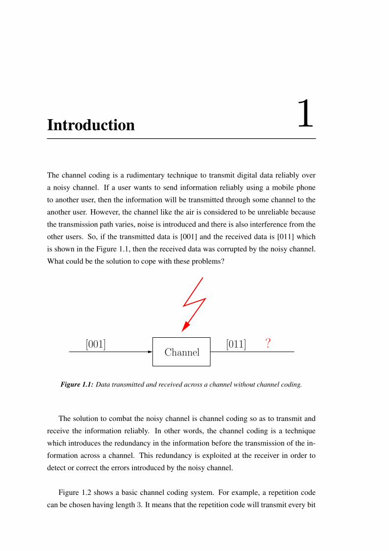
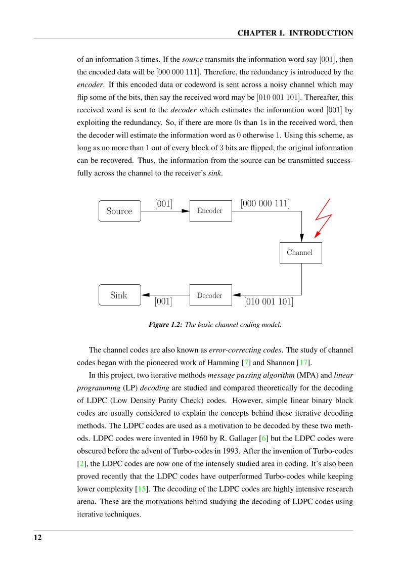
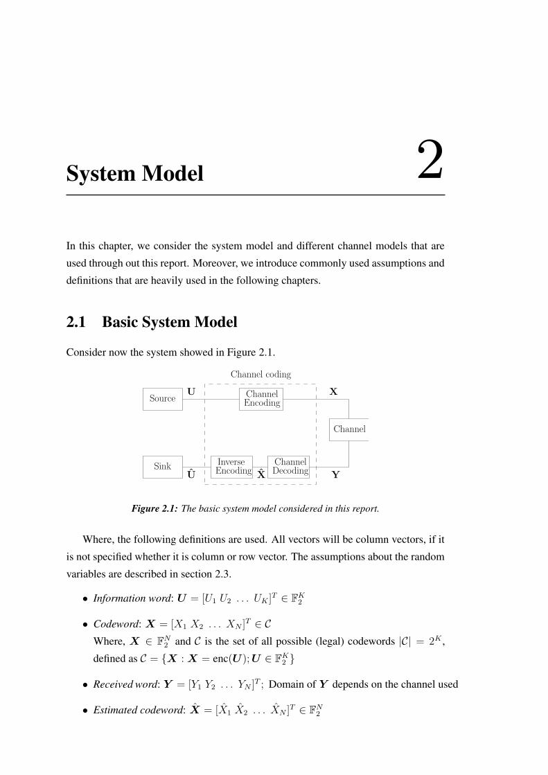
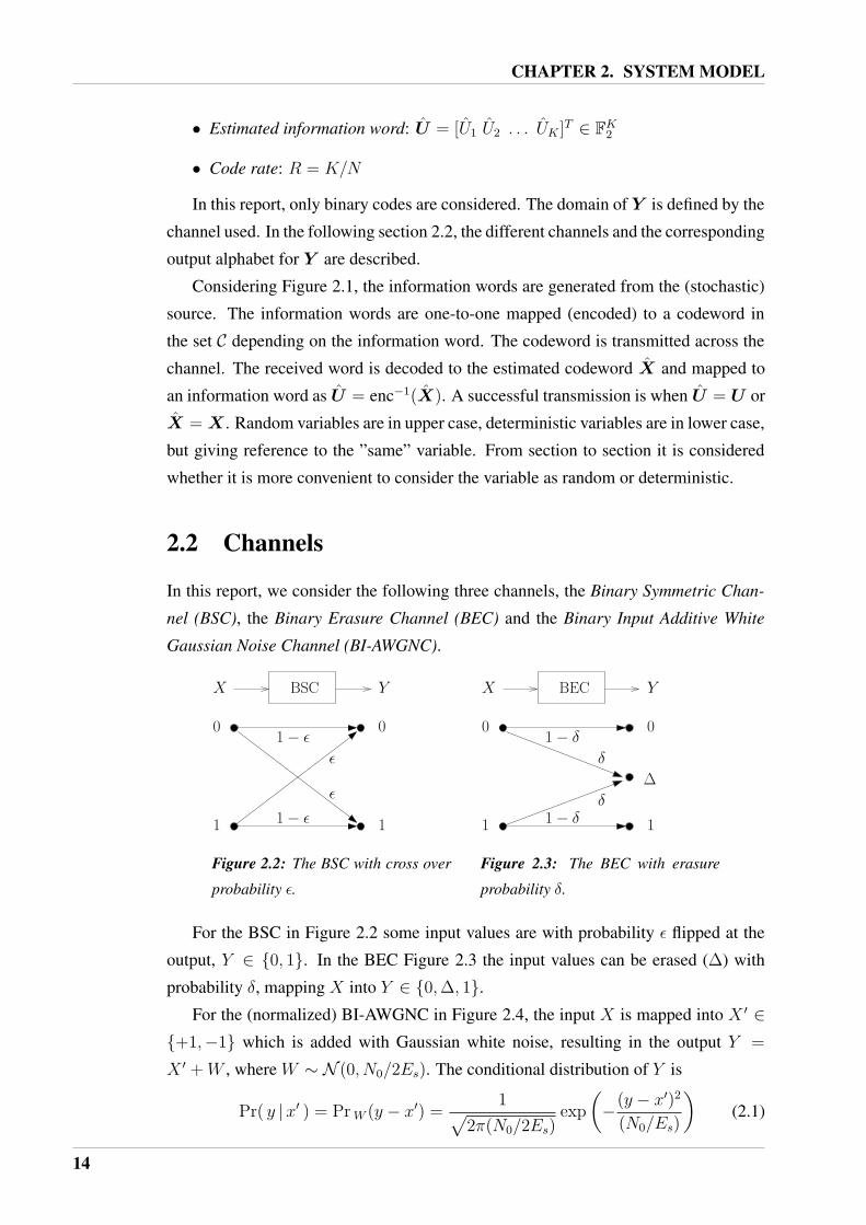
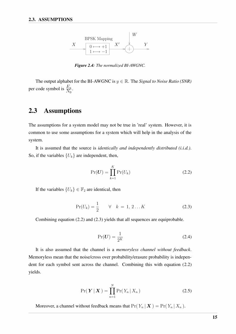
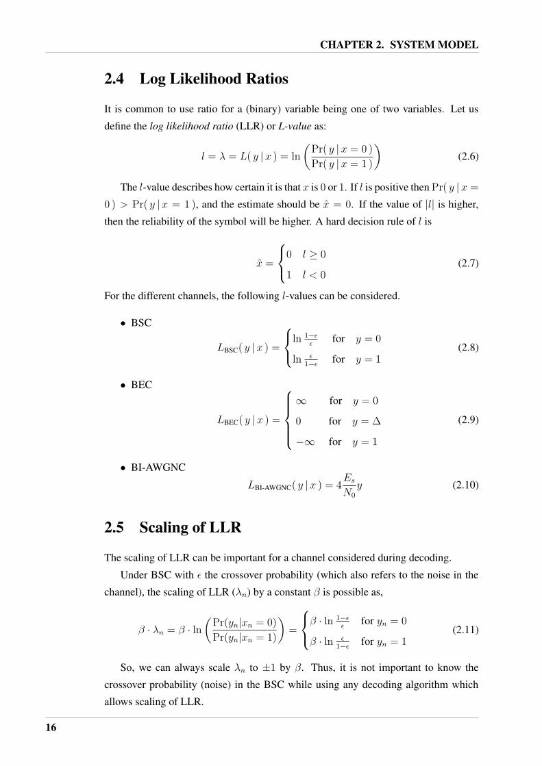
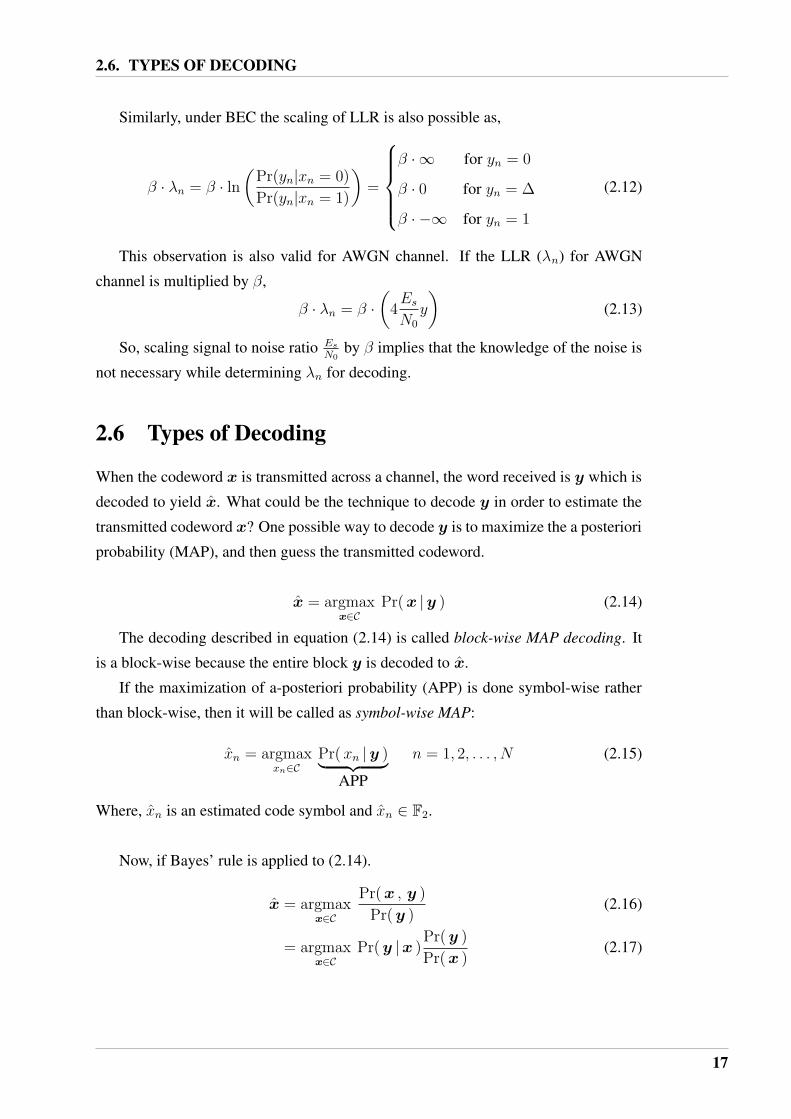
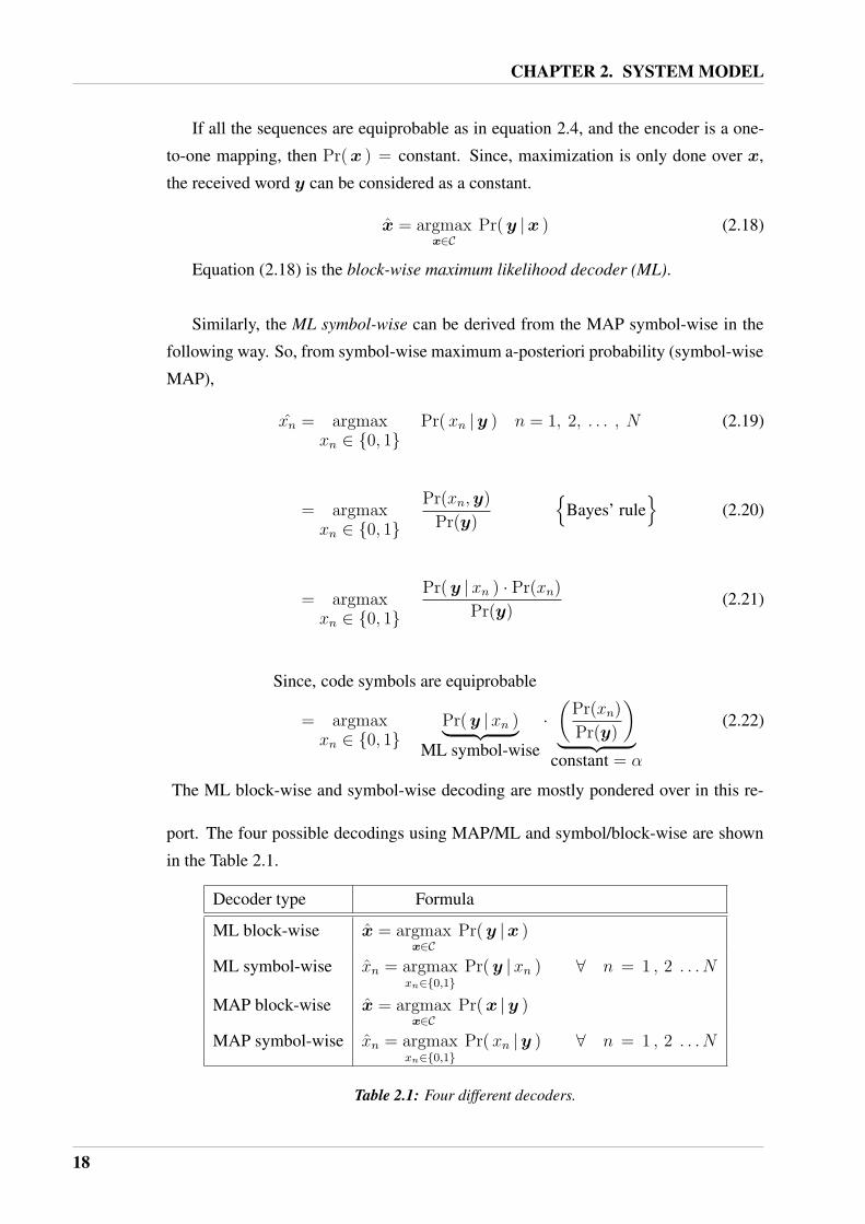
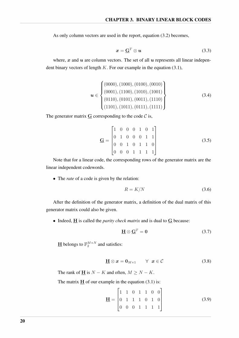
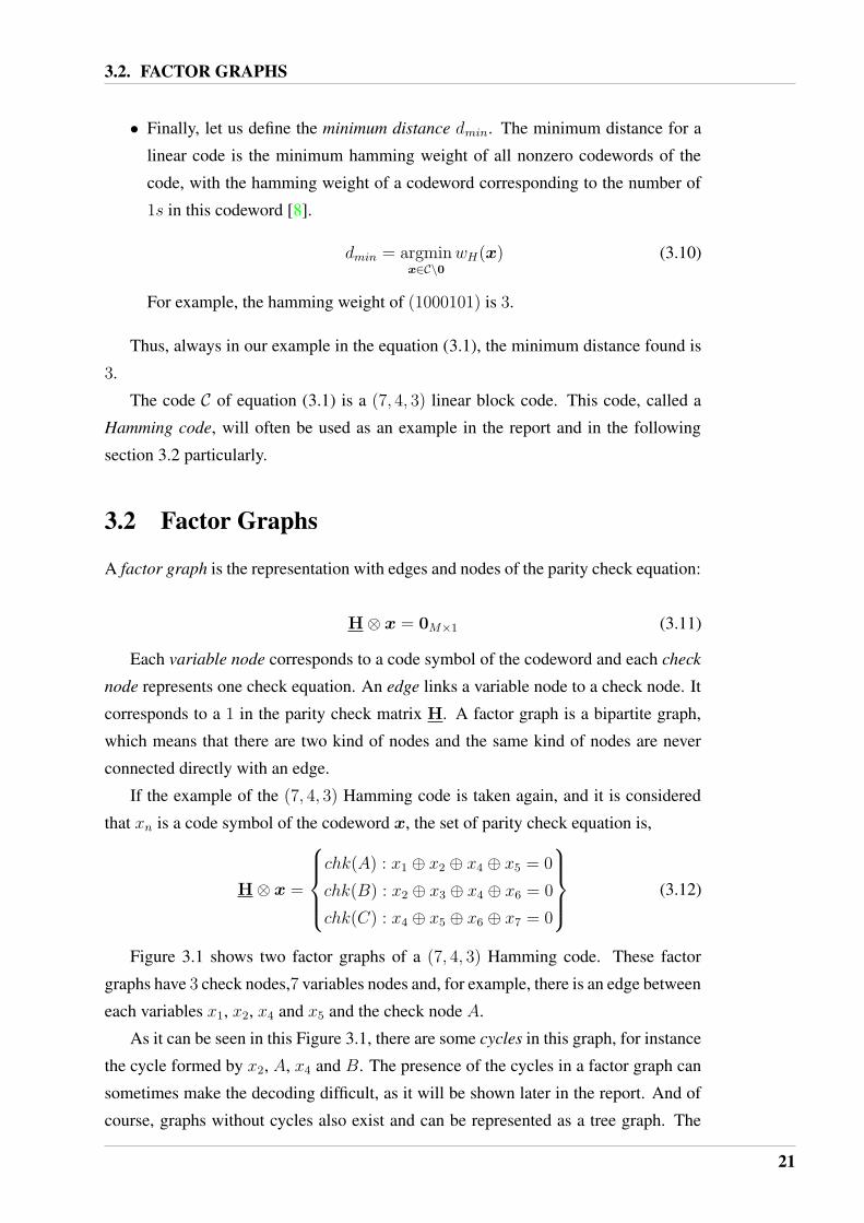
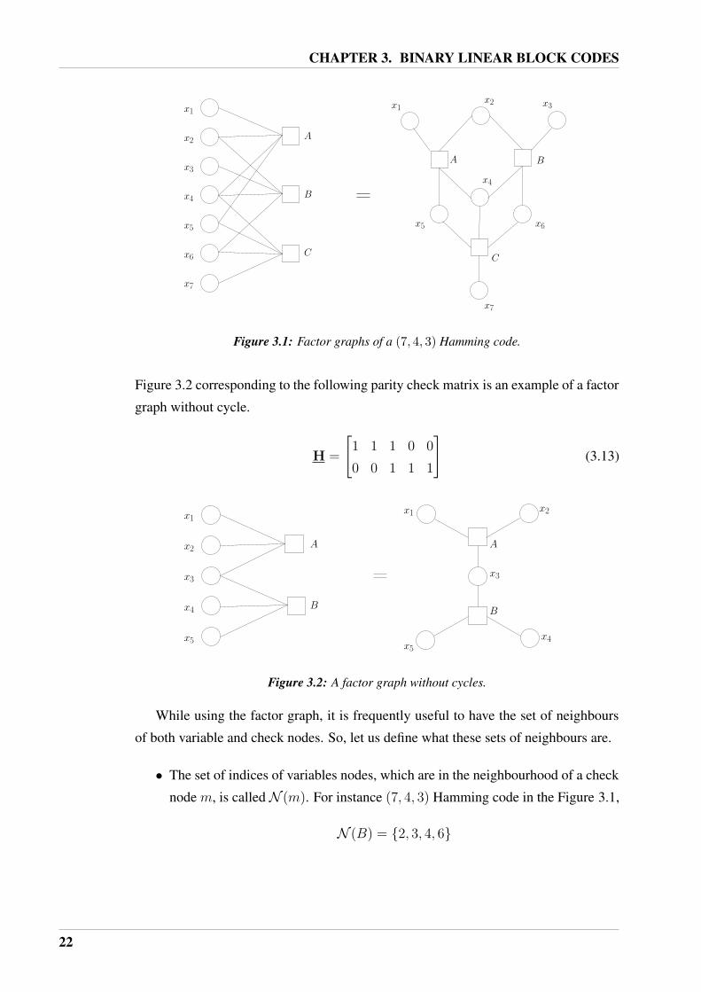
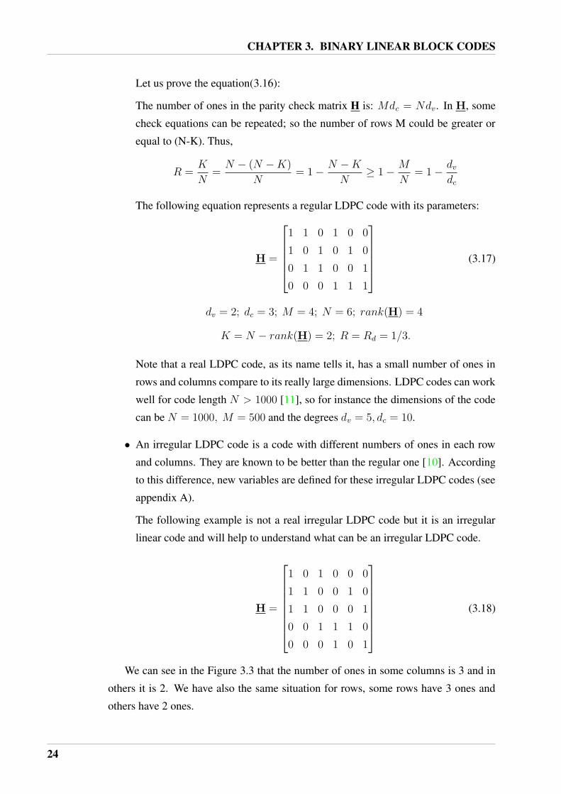
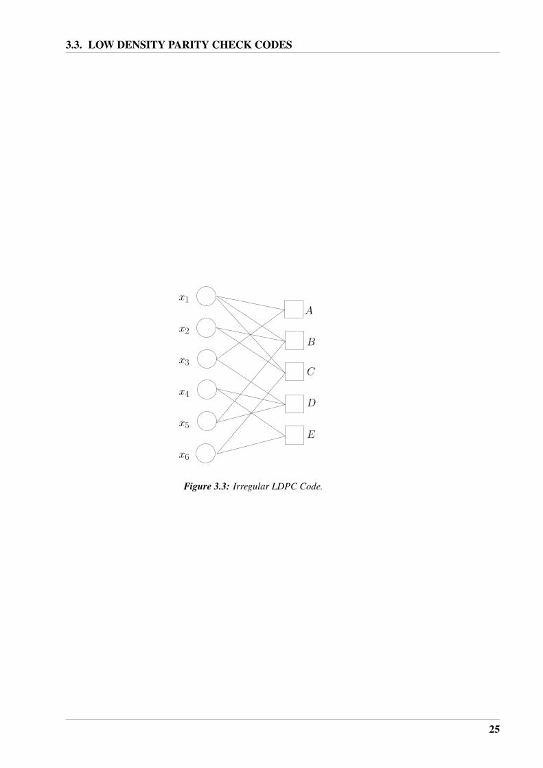


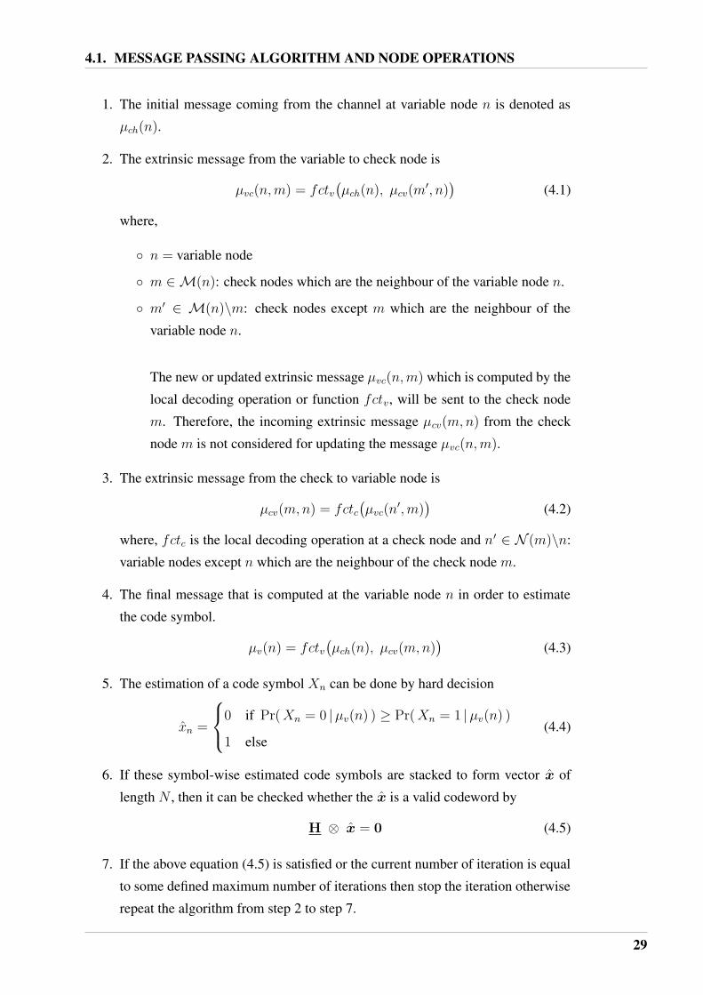
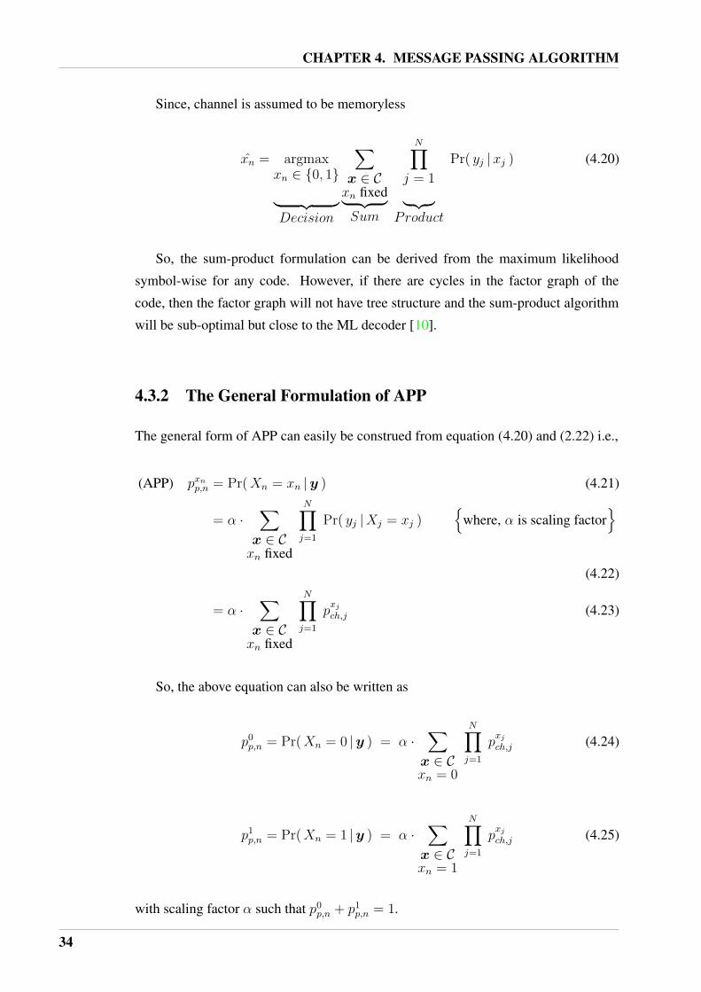
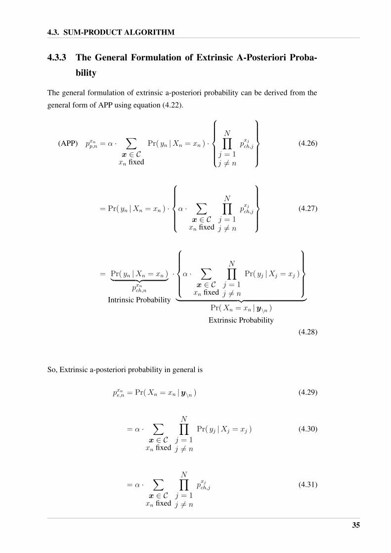


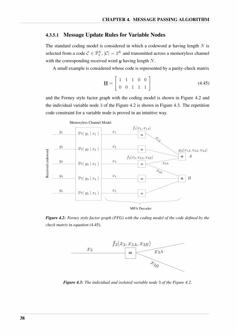
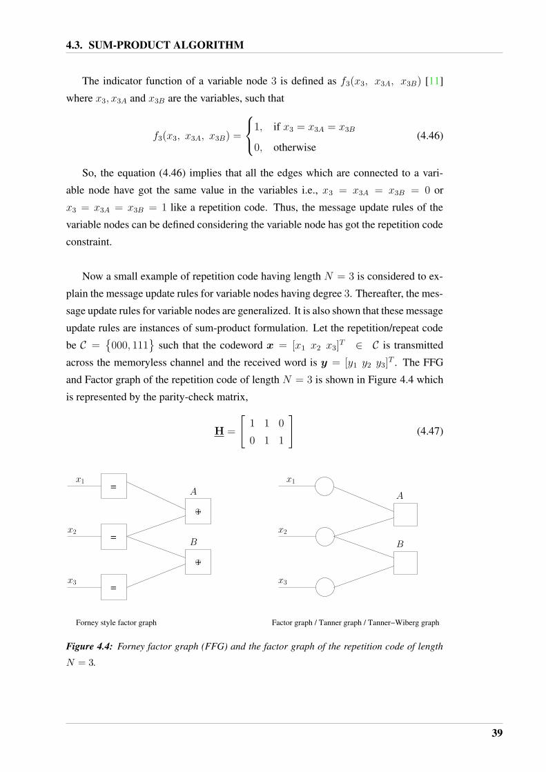
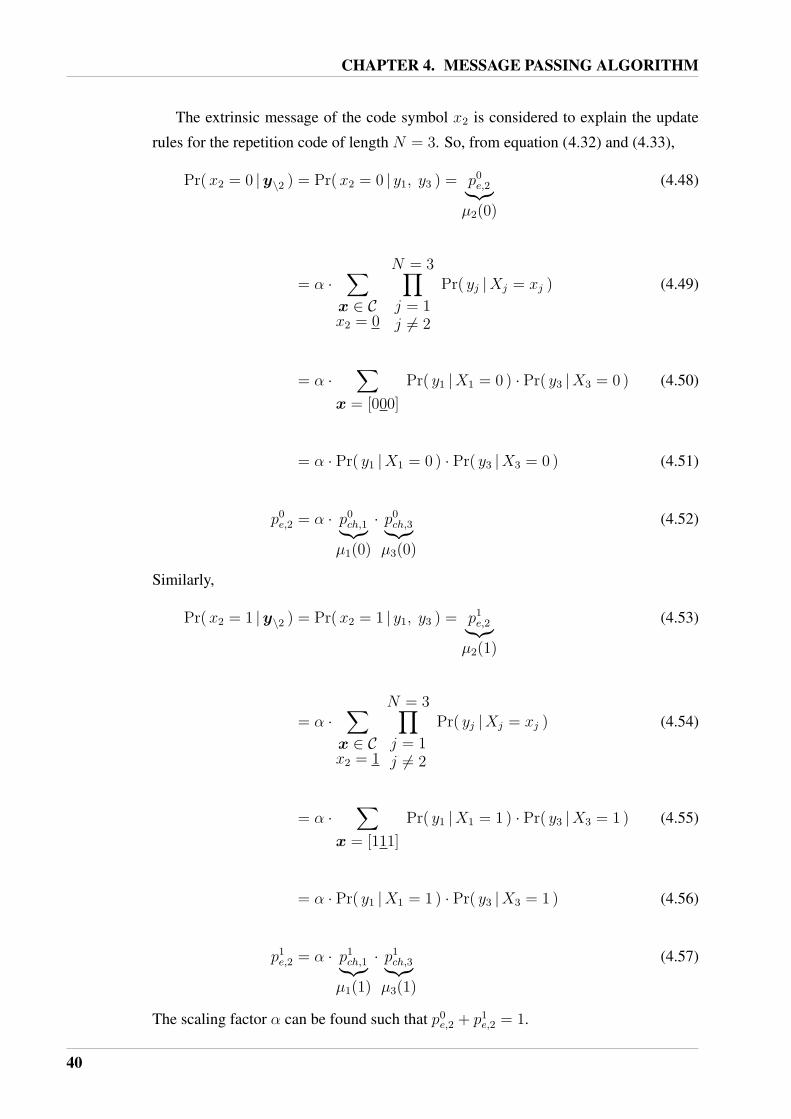
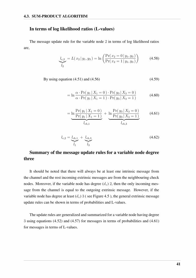
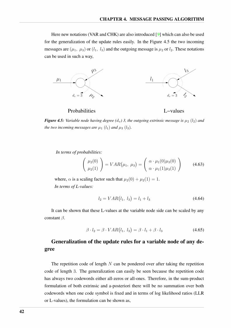
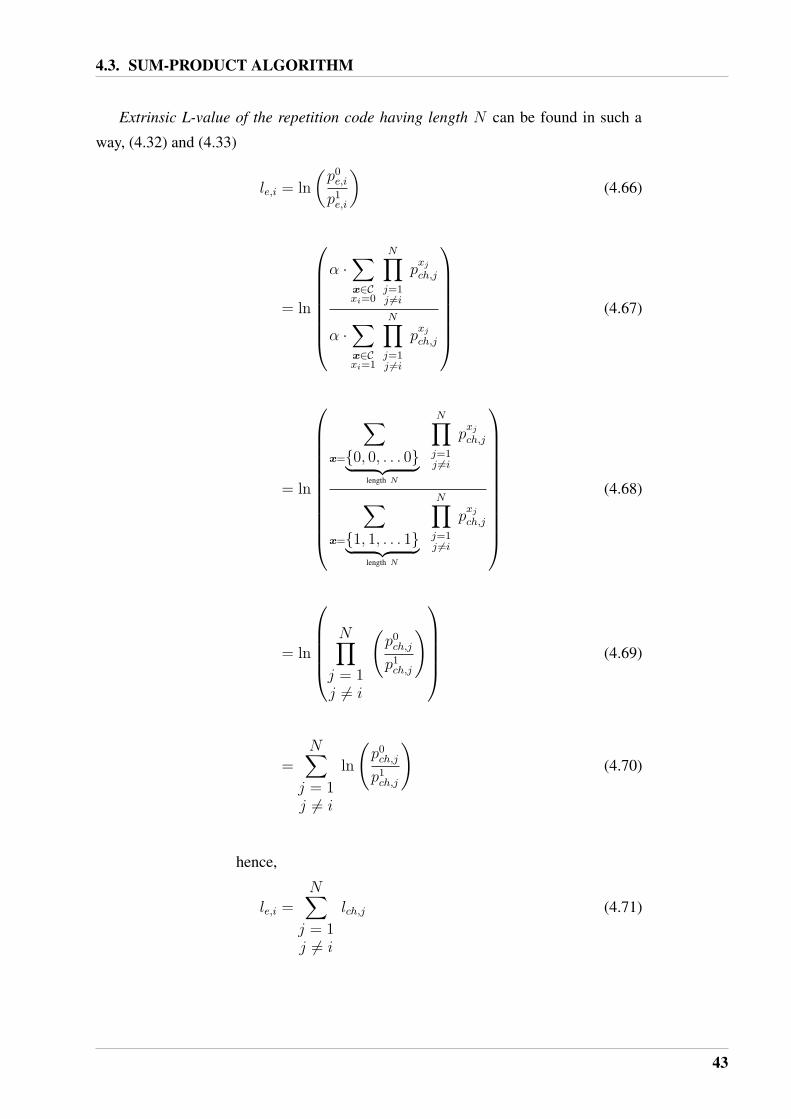
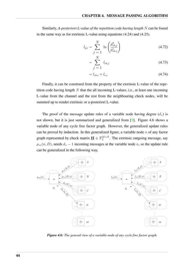
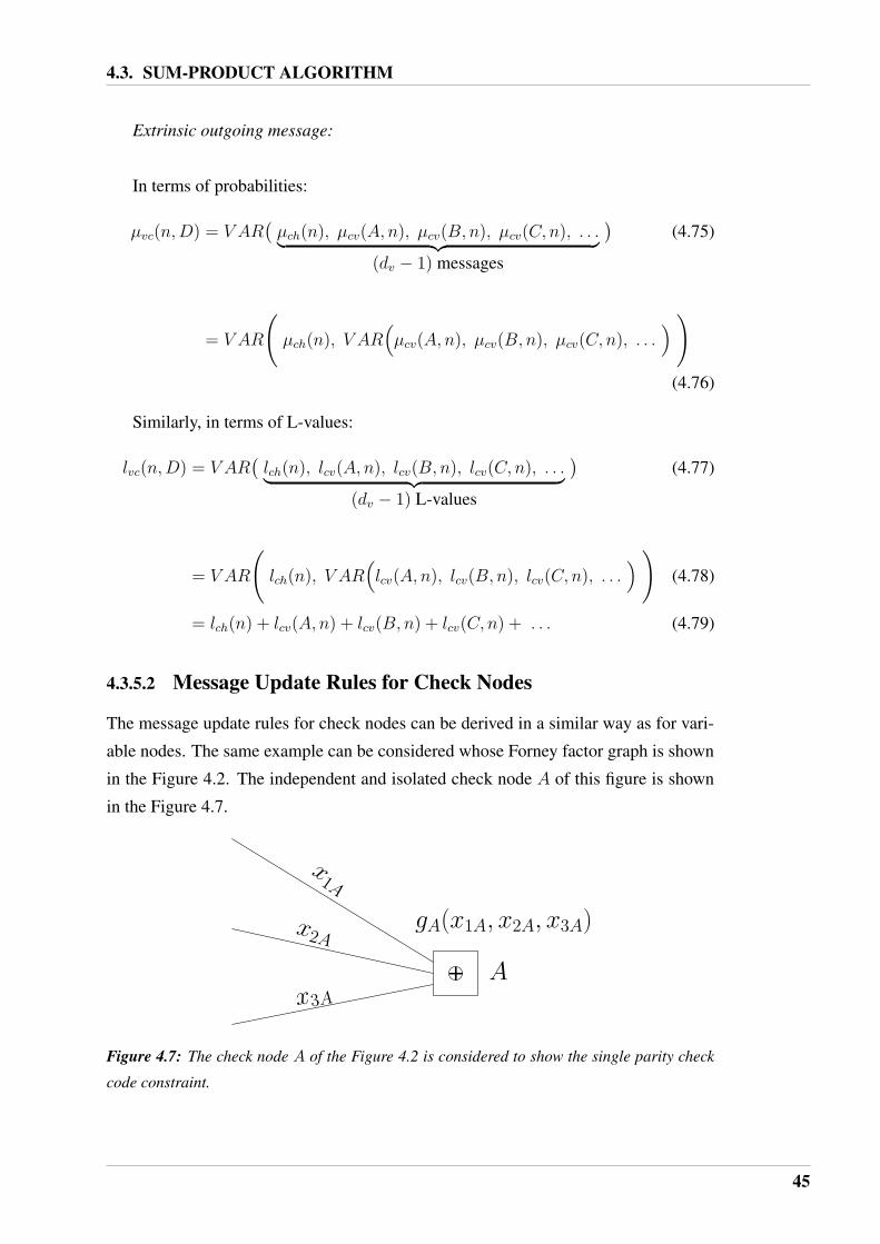
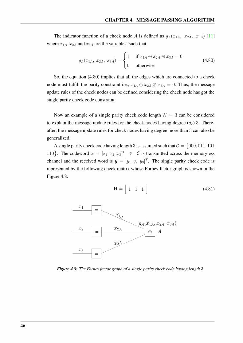
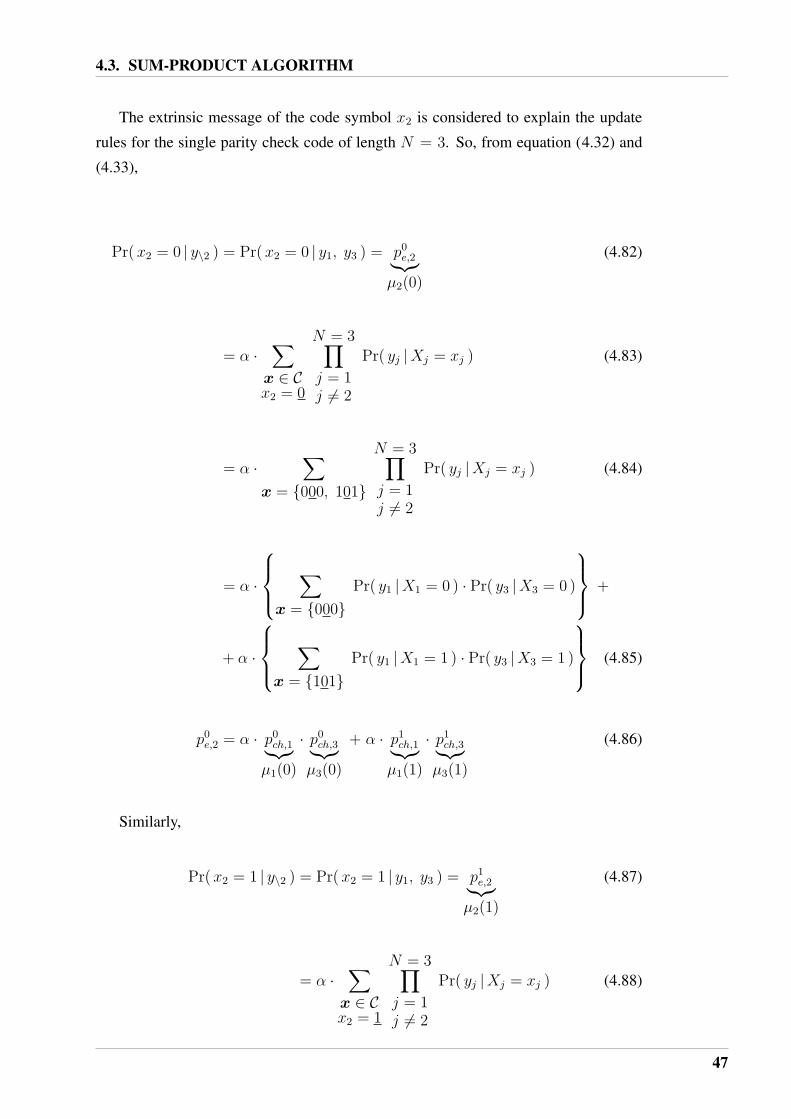
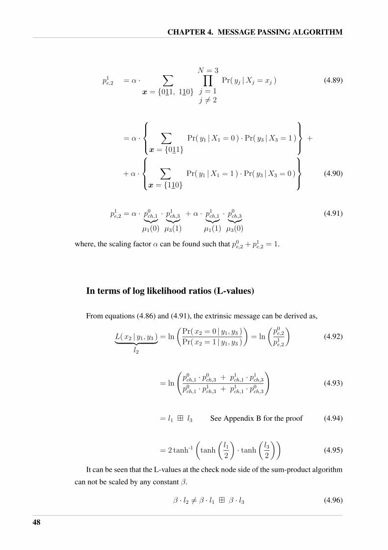
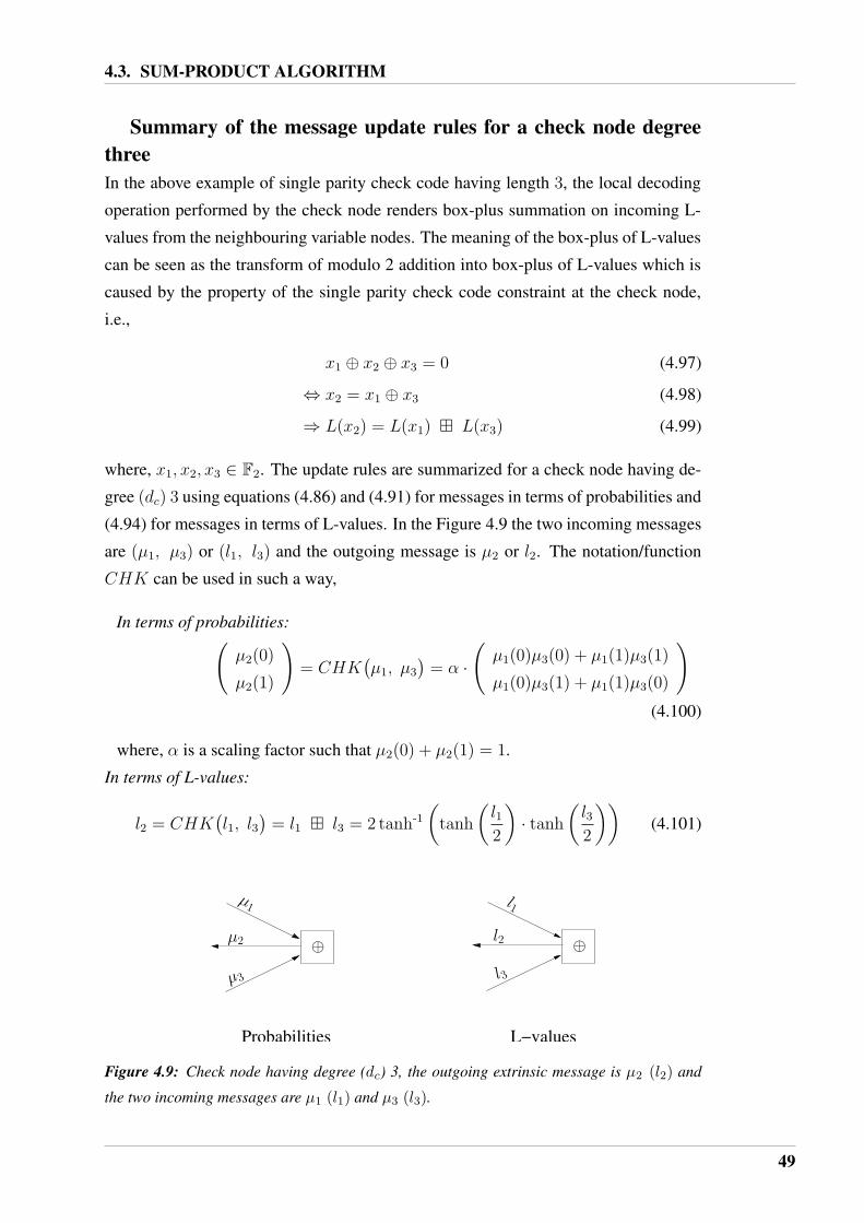
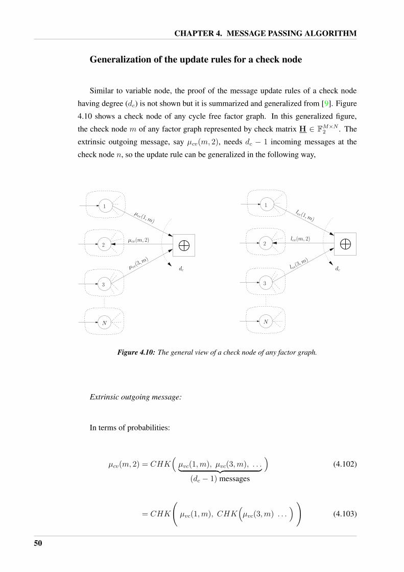
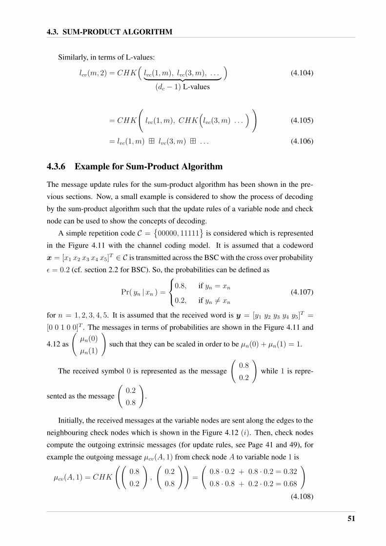

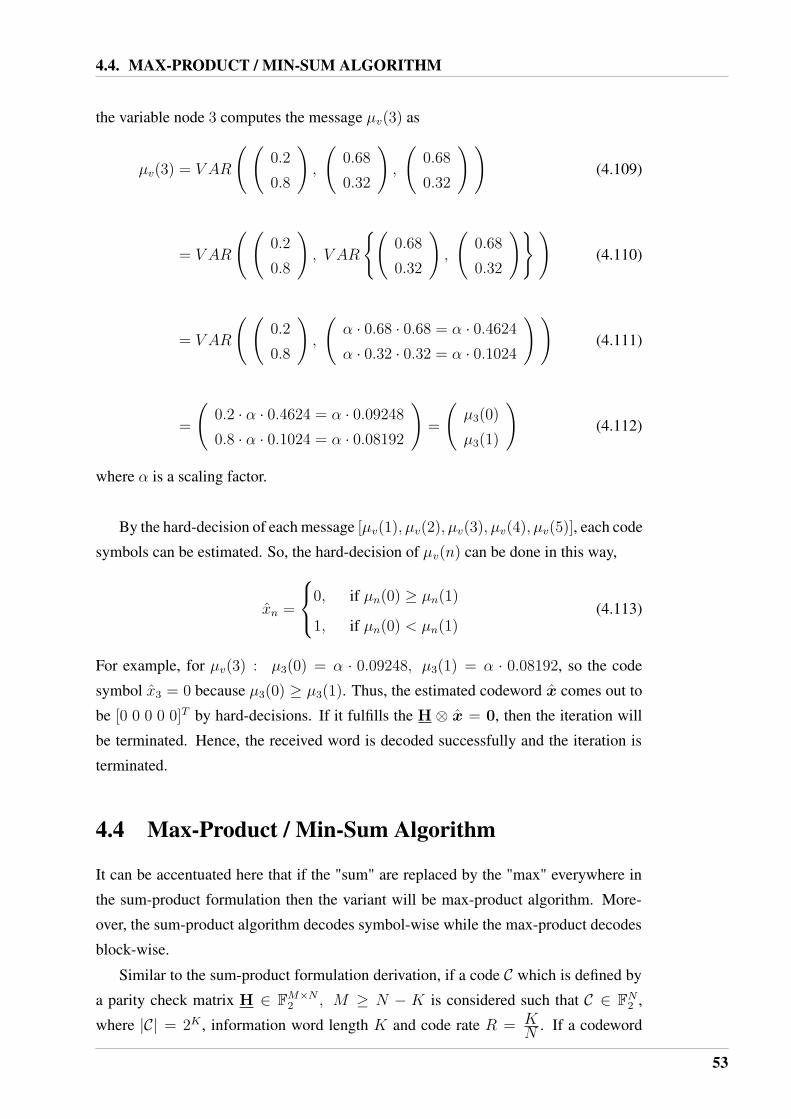
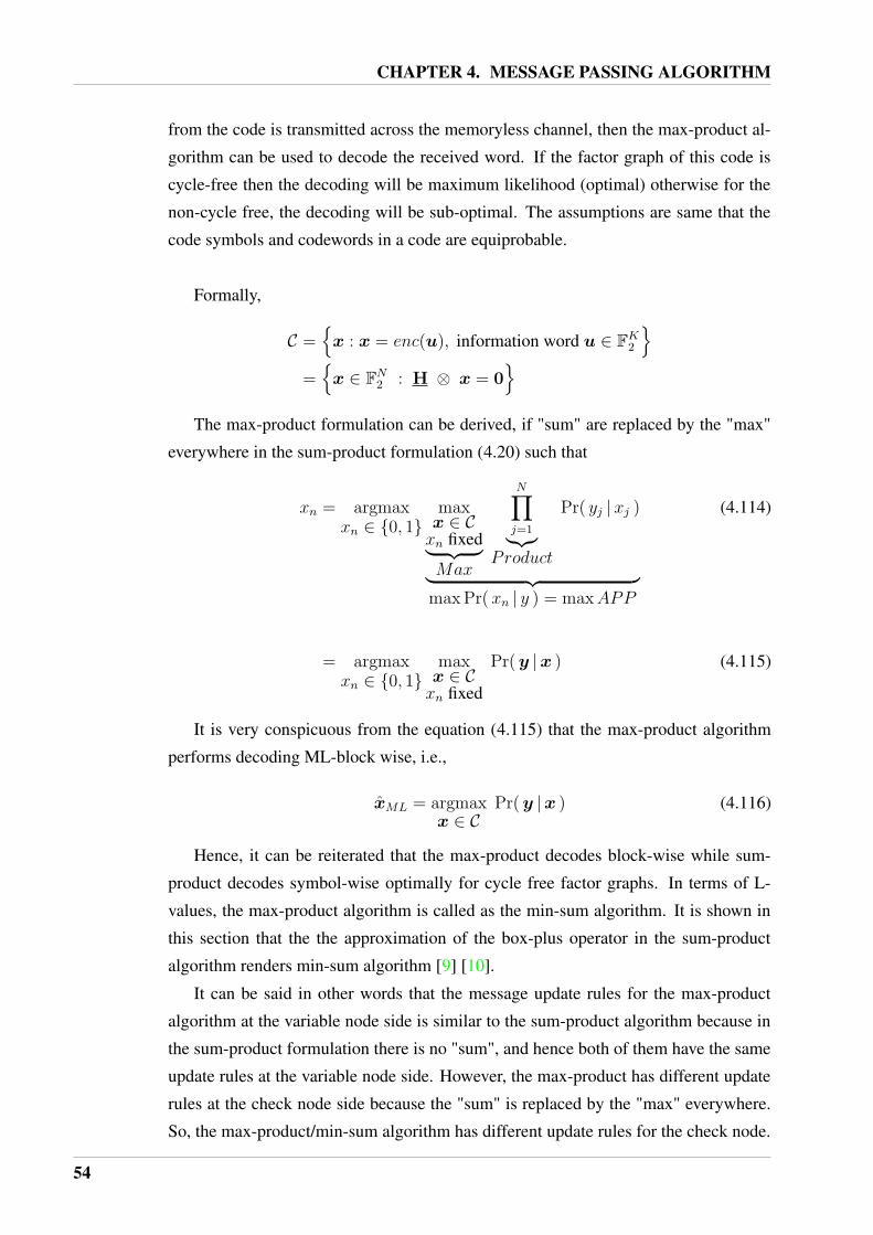
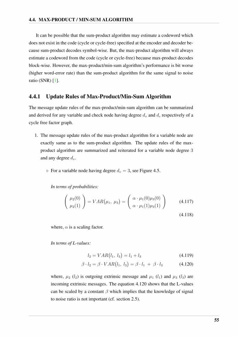
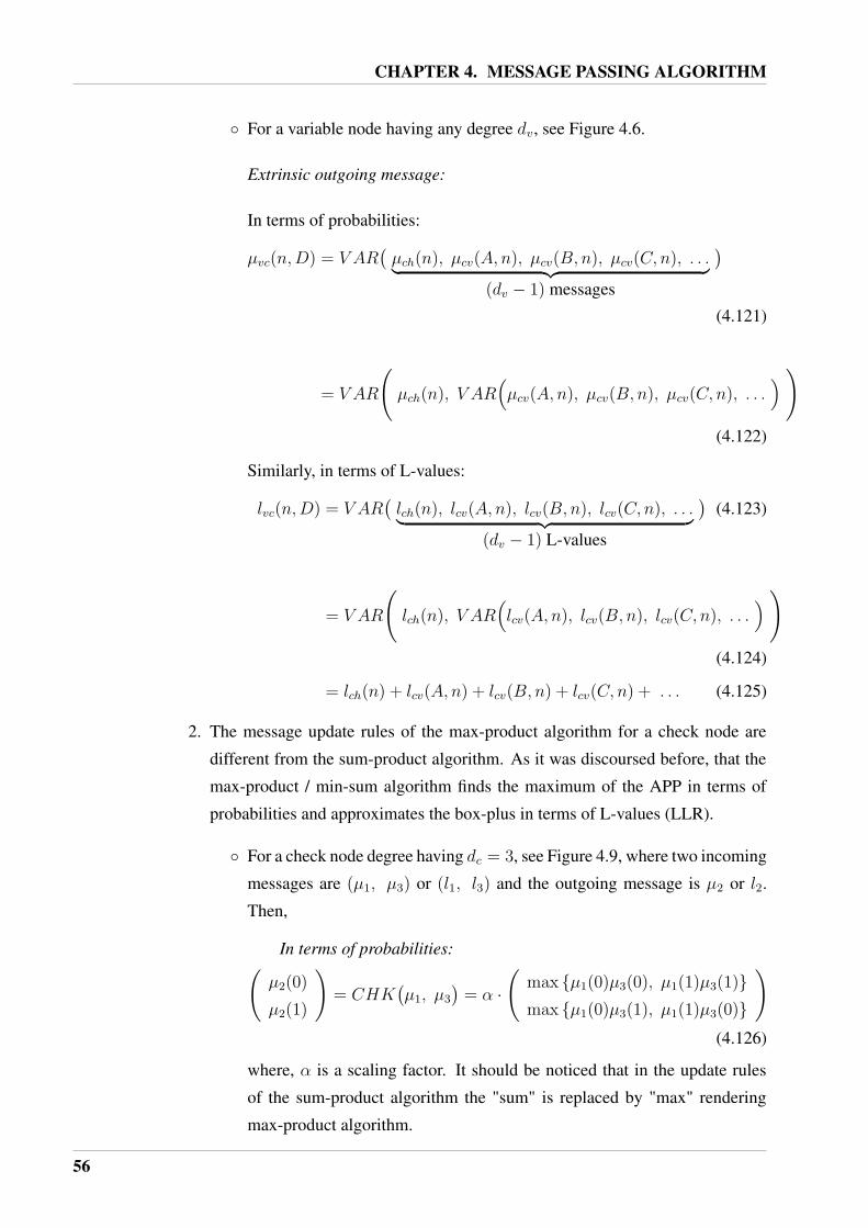
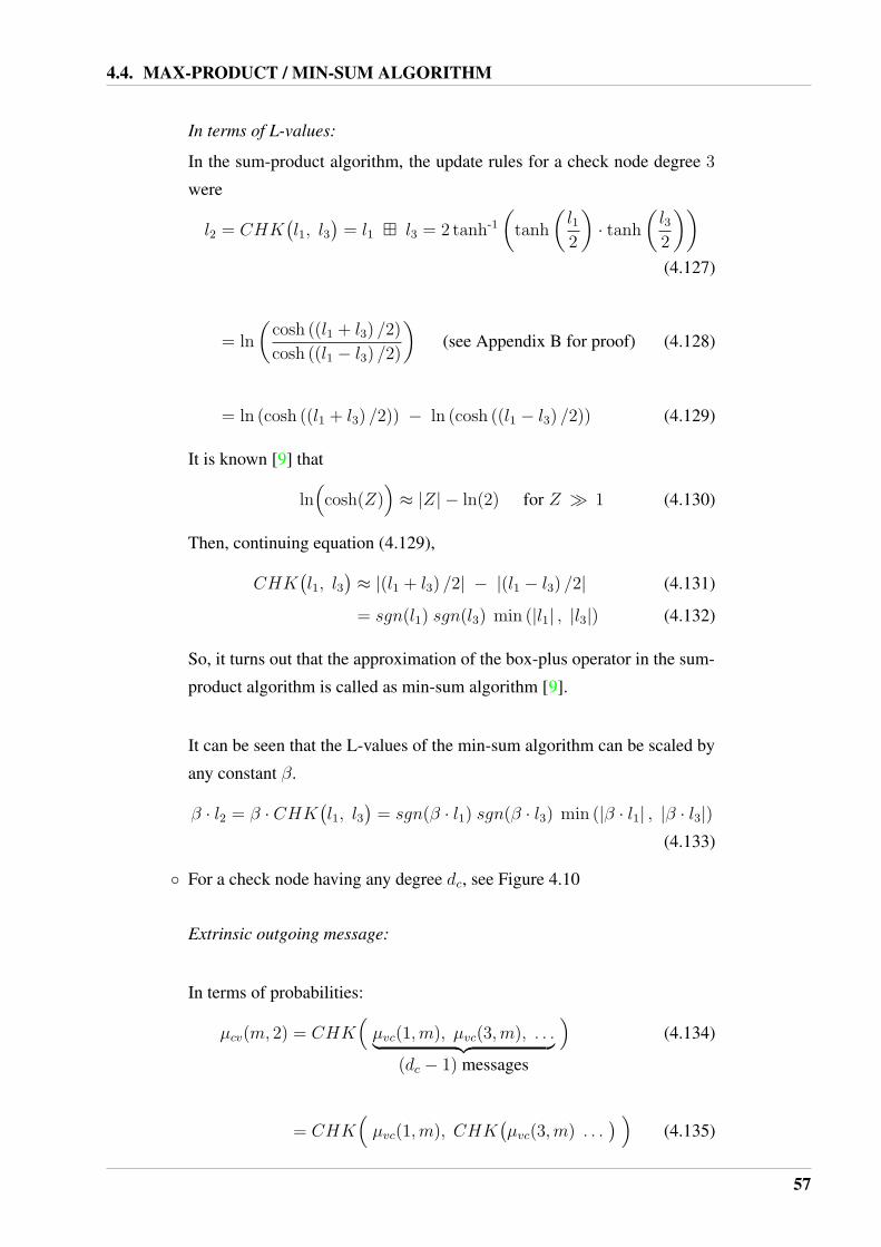
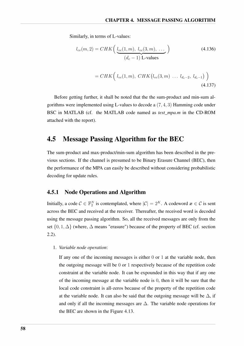
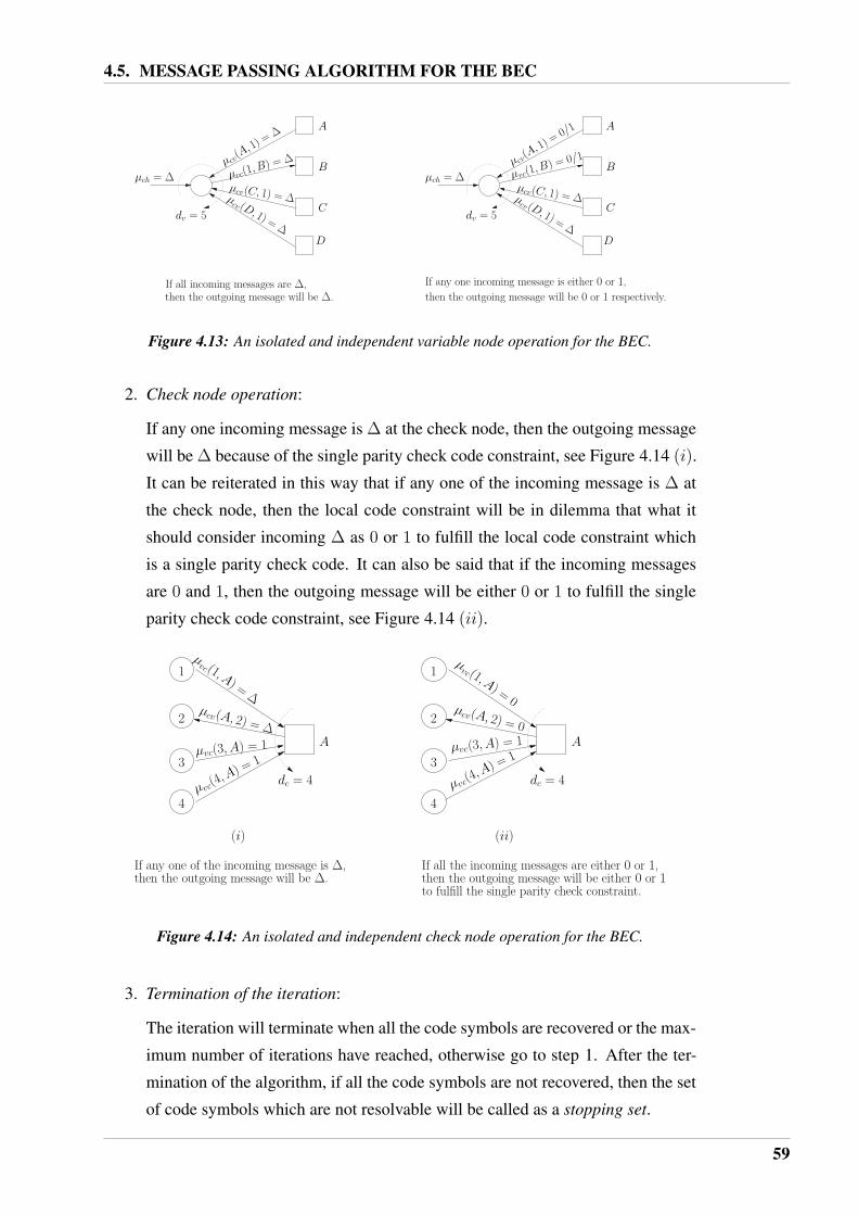
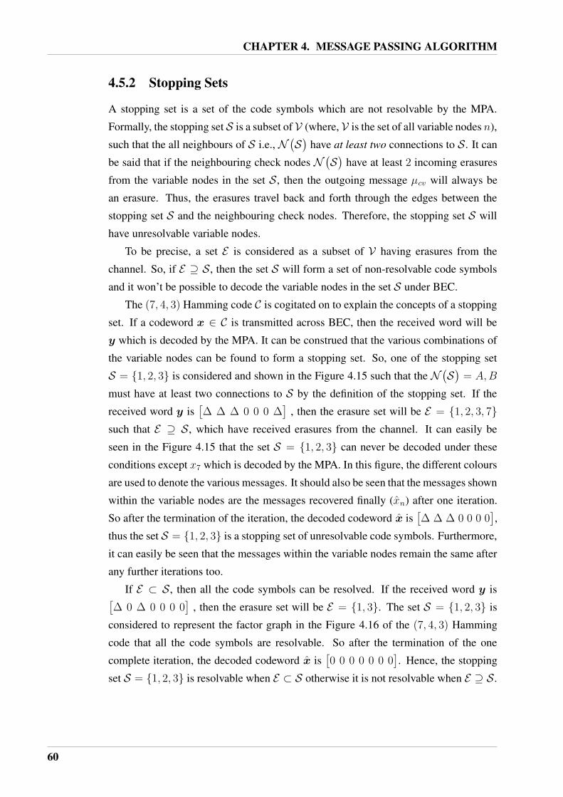


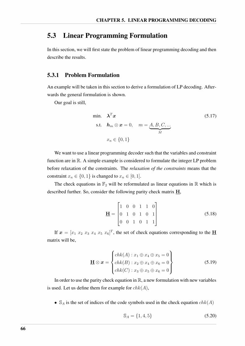
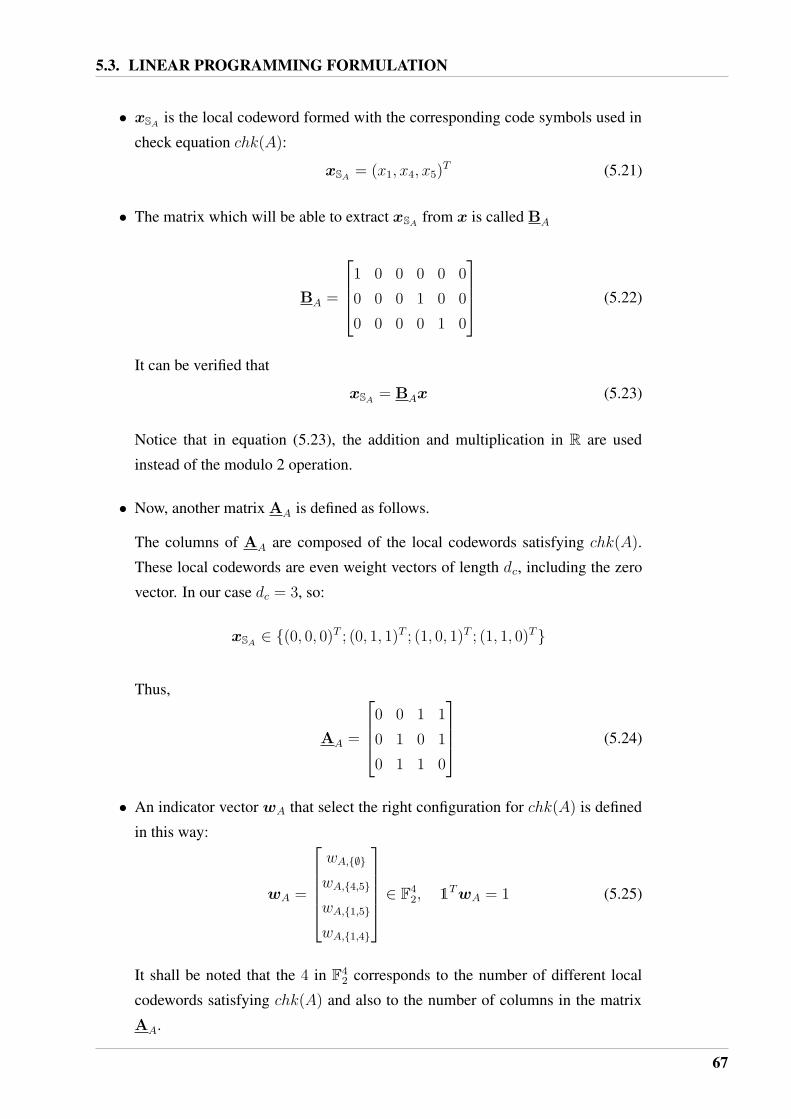
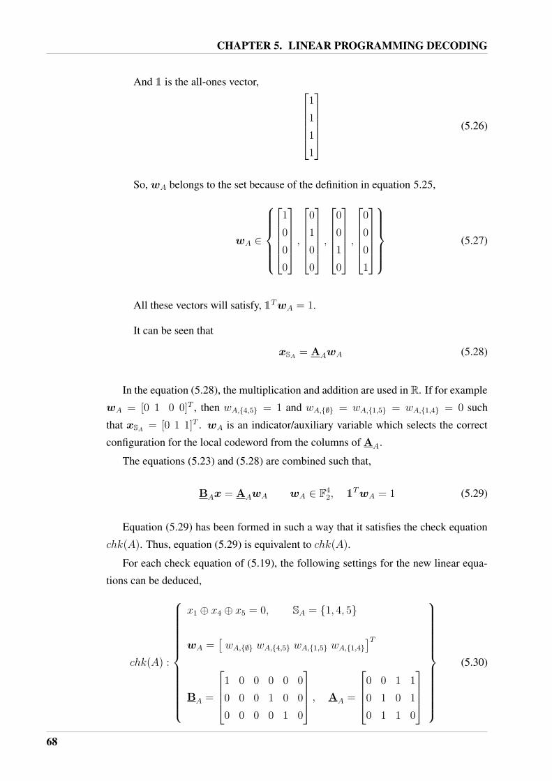
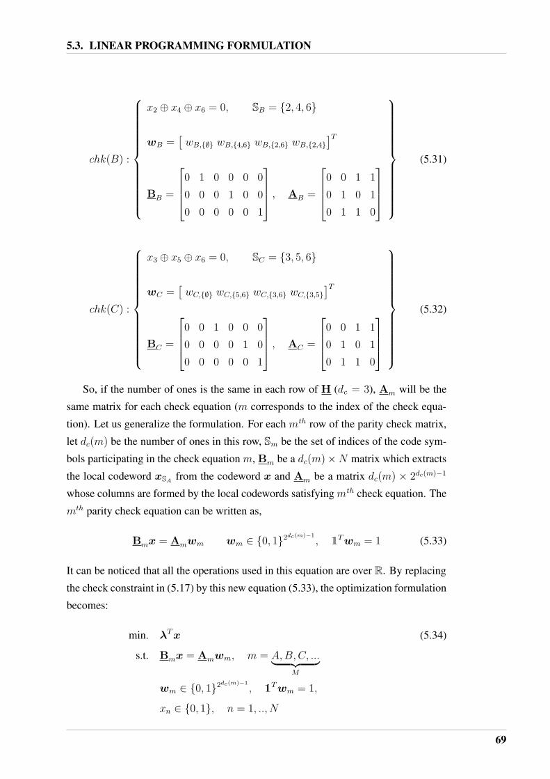

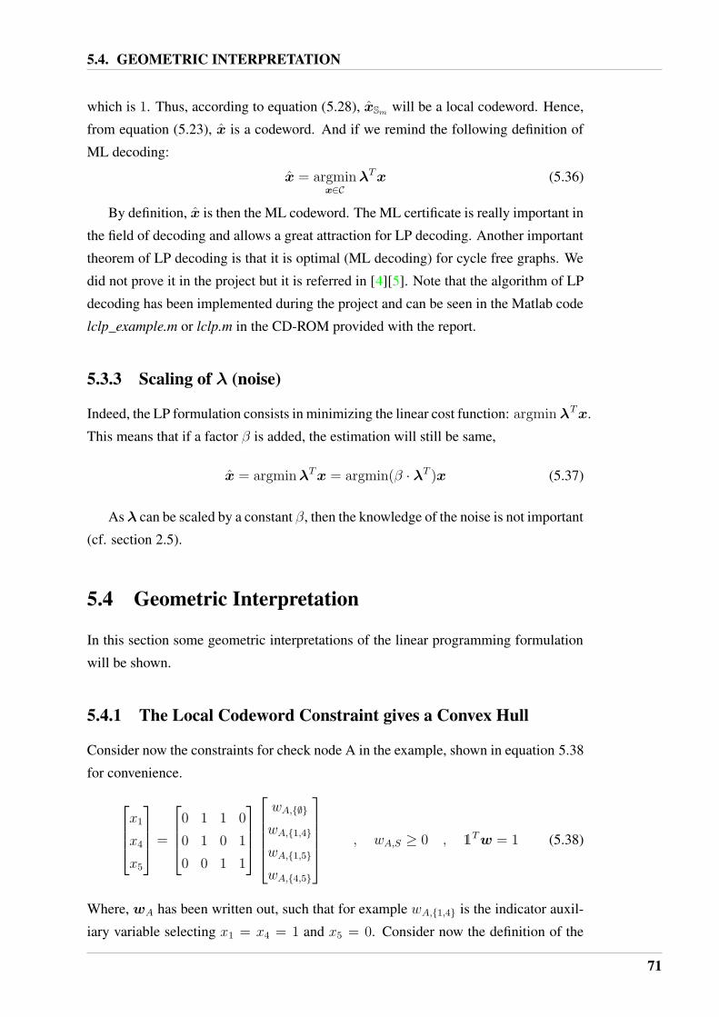
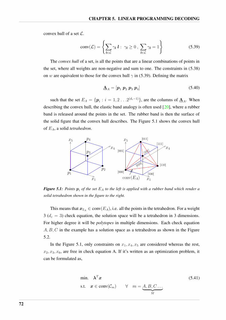
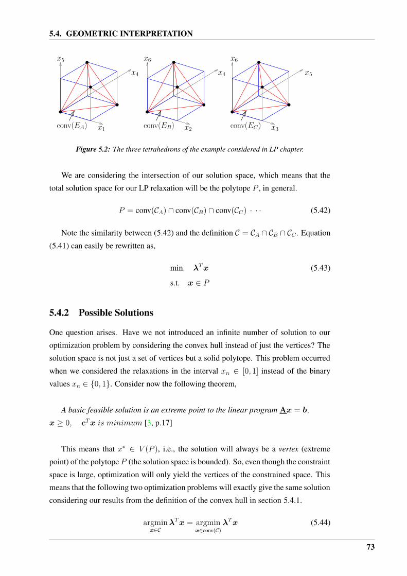
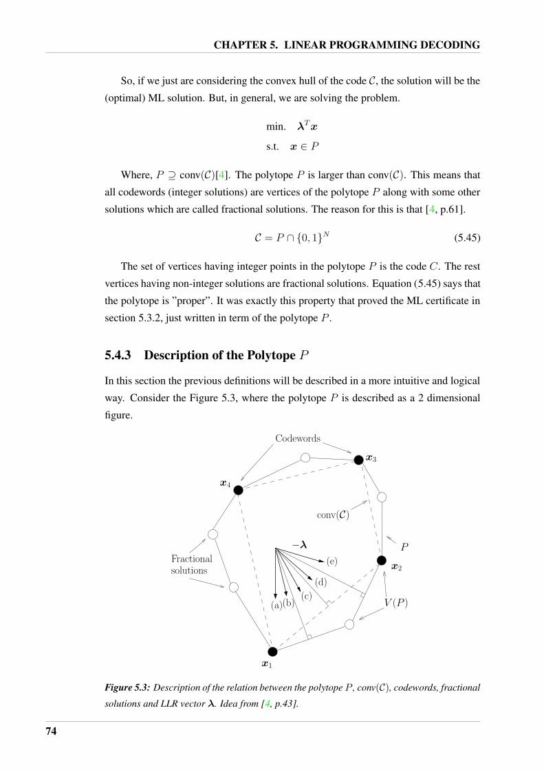

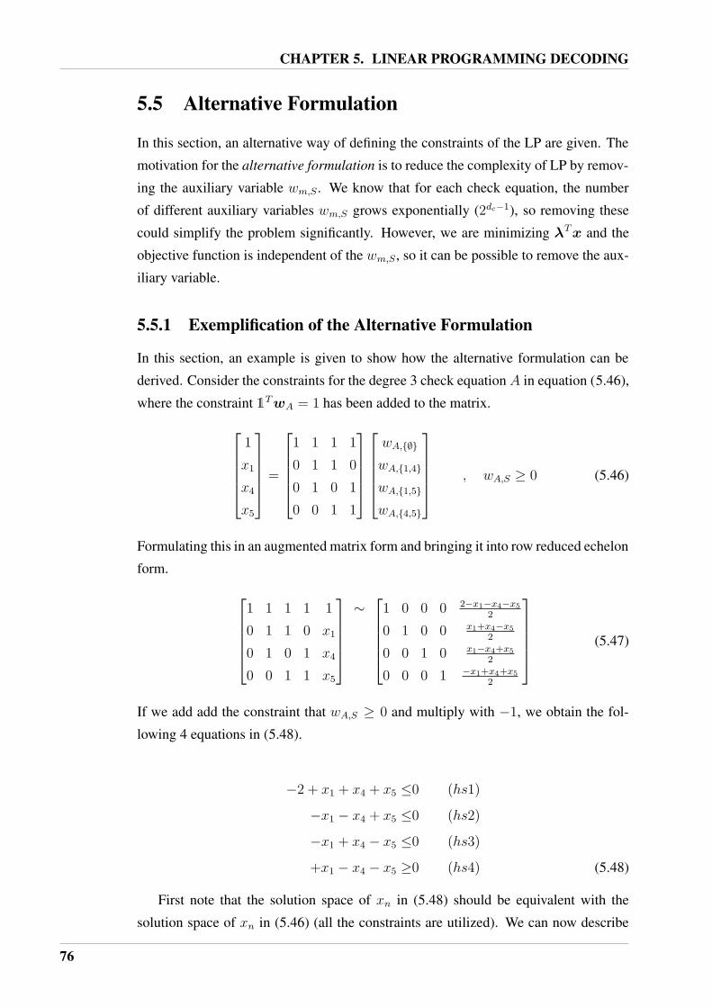
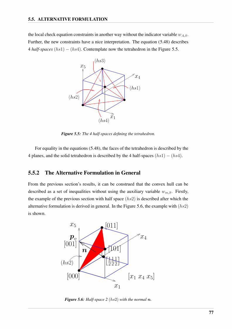


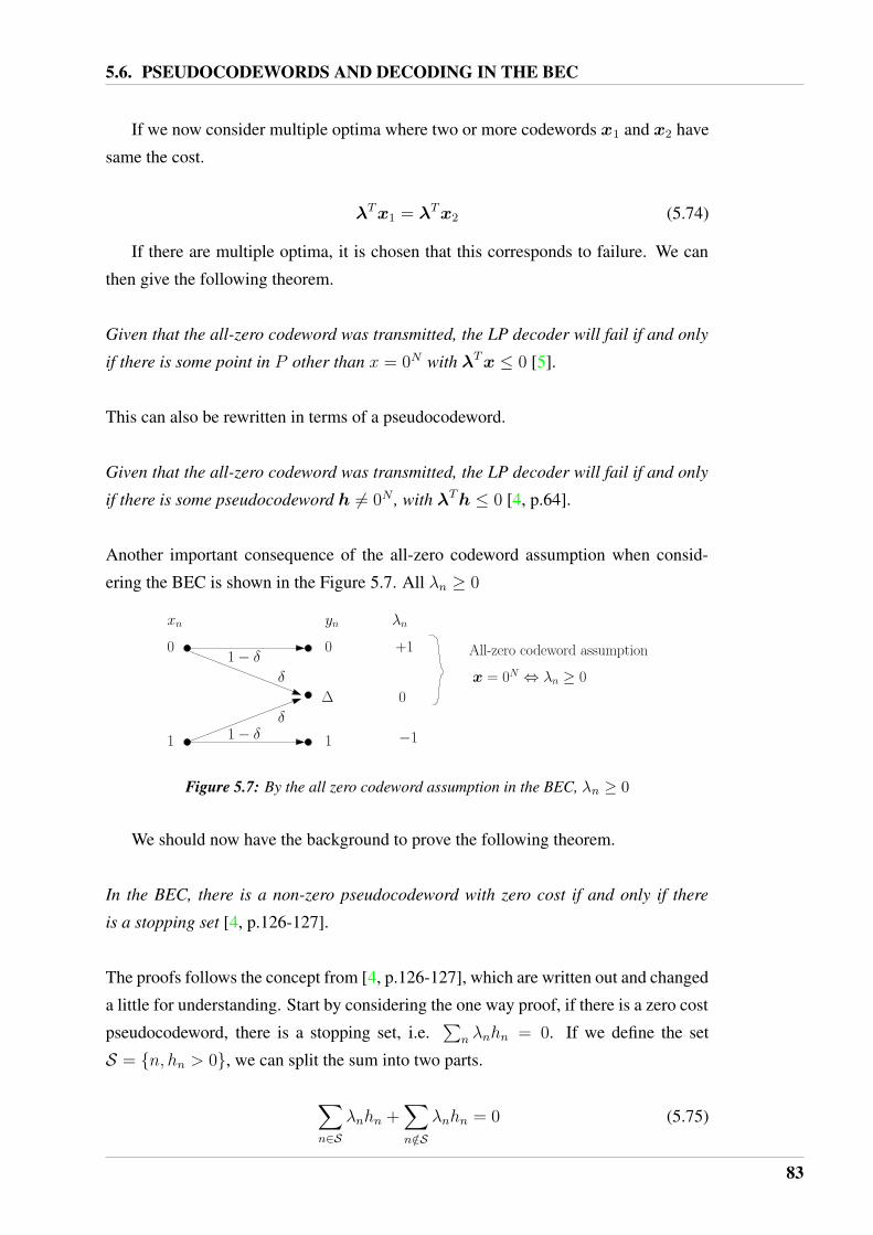

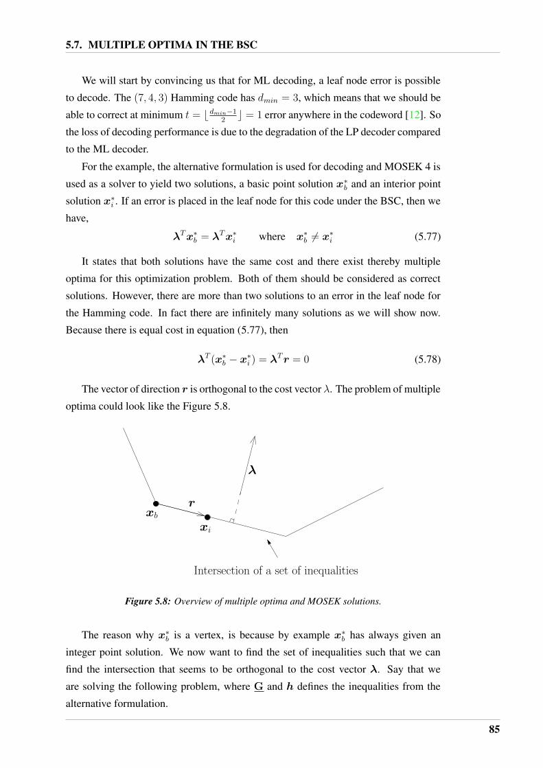
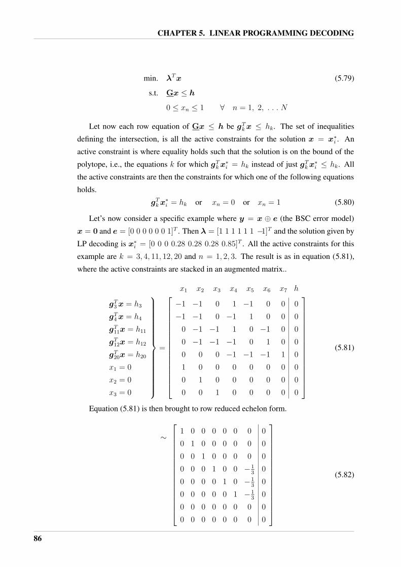
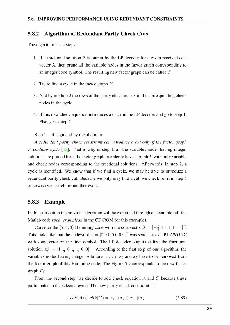
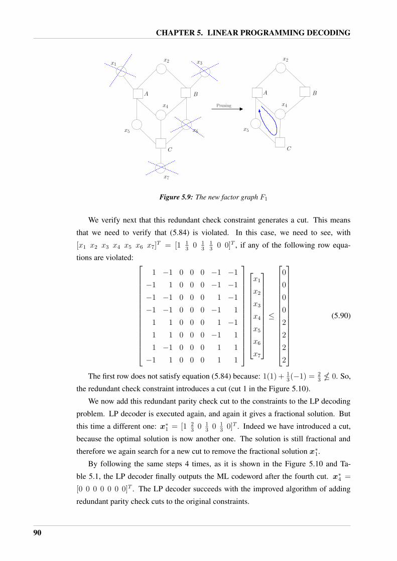
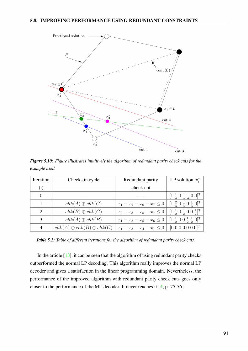

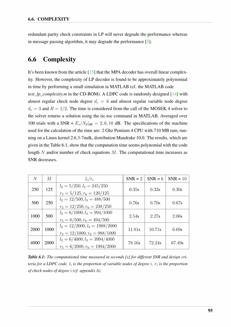

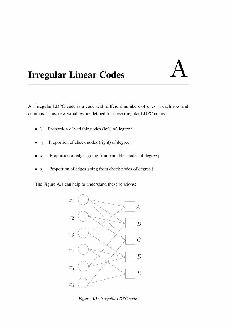
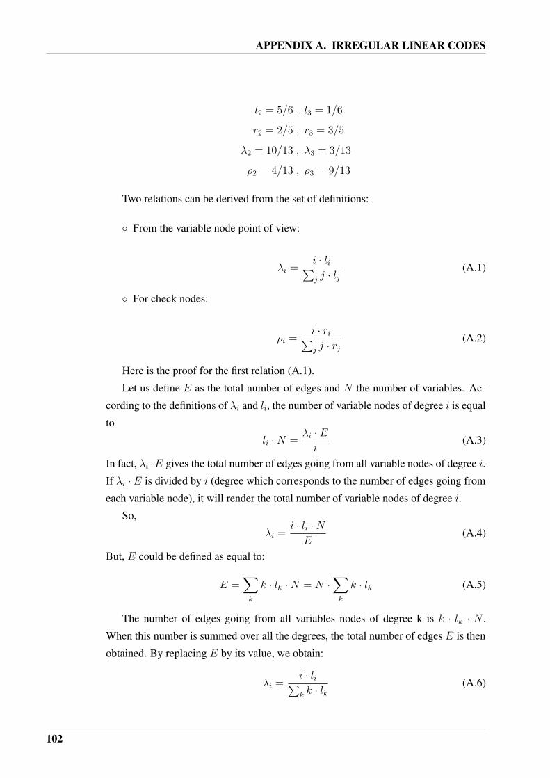
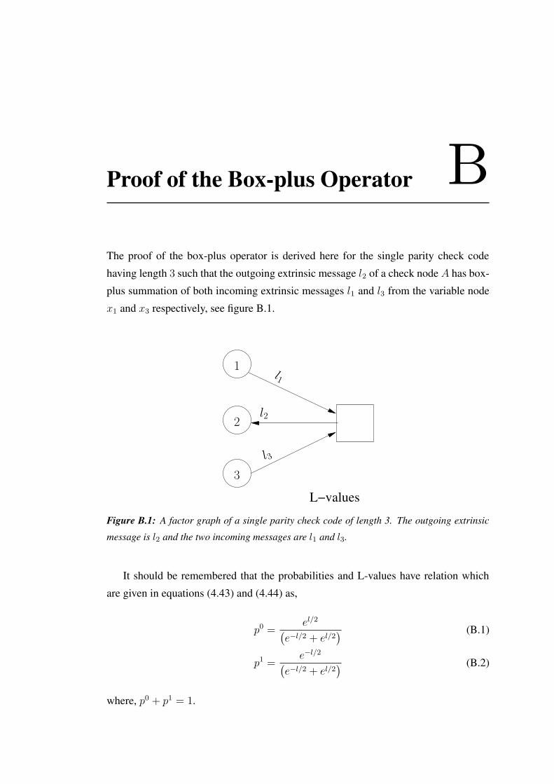


![A decoding algorithm for 2D convolutional codes over the erasure channel · 2020-06-19 · arXiv:2006.10527v1 [cs.IT] 18 Jun 2020 A decoding algorithm for 2D convolutional codes over](https://static.documents.pub/doc/80x56/5f52ef4477b927177a29f16d/a-decoding-algorithm-for-2d-convolutional-codes-over-the-erasure-channel-2020-06-19.jpg)


